Evaluating the enhanced sampling rate for turbulence measurement with a wind lidar profiler

This study evaluates the impact of an enhanced sampling rate on turbulence measurements using the Vaisala WindCube v2.1 lidar profiler. A prototype configuration, sampling 4 times faster than the commercial setup, was compared to the commercial WindCube v2.1, with reference measurements provided by a 2D sonic anemometer mounted on a measurement mast. Over the 47 d experiment, the prototype configuration showed performance similar to the commercial setup for key performance indicators (KPIs) like slope and the coefficient of determination of mean wind speed compared to reference measurements, with both configurations meeting the “best-practice” threshold. However, for mean wind speed differences, the commercial configuration met the best-practice level, while the prototype met the “minimum-acceptance” criterion. Additionally, the data availability of the prototype configuration was 0.5 % lower than that of the commercial configuration. Moreover, the increased sampling rate of the prototype lidar resulted in higher mean variance in instrumental noise compared to that of the commercial configuration. Despite this limitation, the mean noise-corrected along-wind variance measured by the prototype lidar was approximately 7 % higher than that of the commercial lidar. This effect was especially evident at higher wind speeds. Error metrics for the noise-corrected along-wind standard deviation in the prototype lidar were approximately 25 % lower than those of the commercial configuration. However, the observed improvements to the prototype configuration in measuring turbulence fell short of expectations due to inherent limitations in the measurement process within the probe, where spatial and temporal filtering effects constrain the detection of turbulence at certain scales.

1 Introduction

Accurate turbulence data enable better understanding and control of flow patterns, optimizing the design, operation, and maintenance of wind energy systems. Turbulence plays a critical role in the wind energy sector because it directly influences the unsteady aerodynamic loads experienced by turbines (e.g., Frandsen, 2007; Mücke et al., 2011; Dimitrov et al., 2017). These fluctuating loads affect the structural integrity and operational stability of wind turbine components. Therefore, precise turbulence measurement is essential for enhancing the efficiency and safety of turbine operations, minimizing wear and tear on vital components, and extending the lifespan of these costly assets. Additionally, improved turbulence characterization can facilitate more precise wind resource assessments, aiding in site selection and the overall planning of wind energy projects (e.g., Yang et al., 2021).

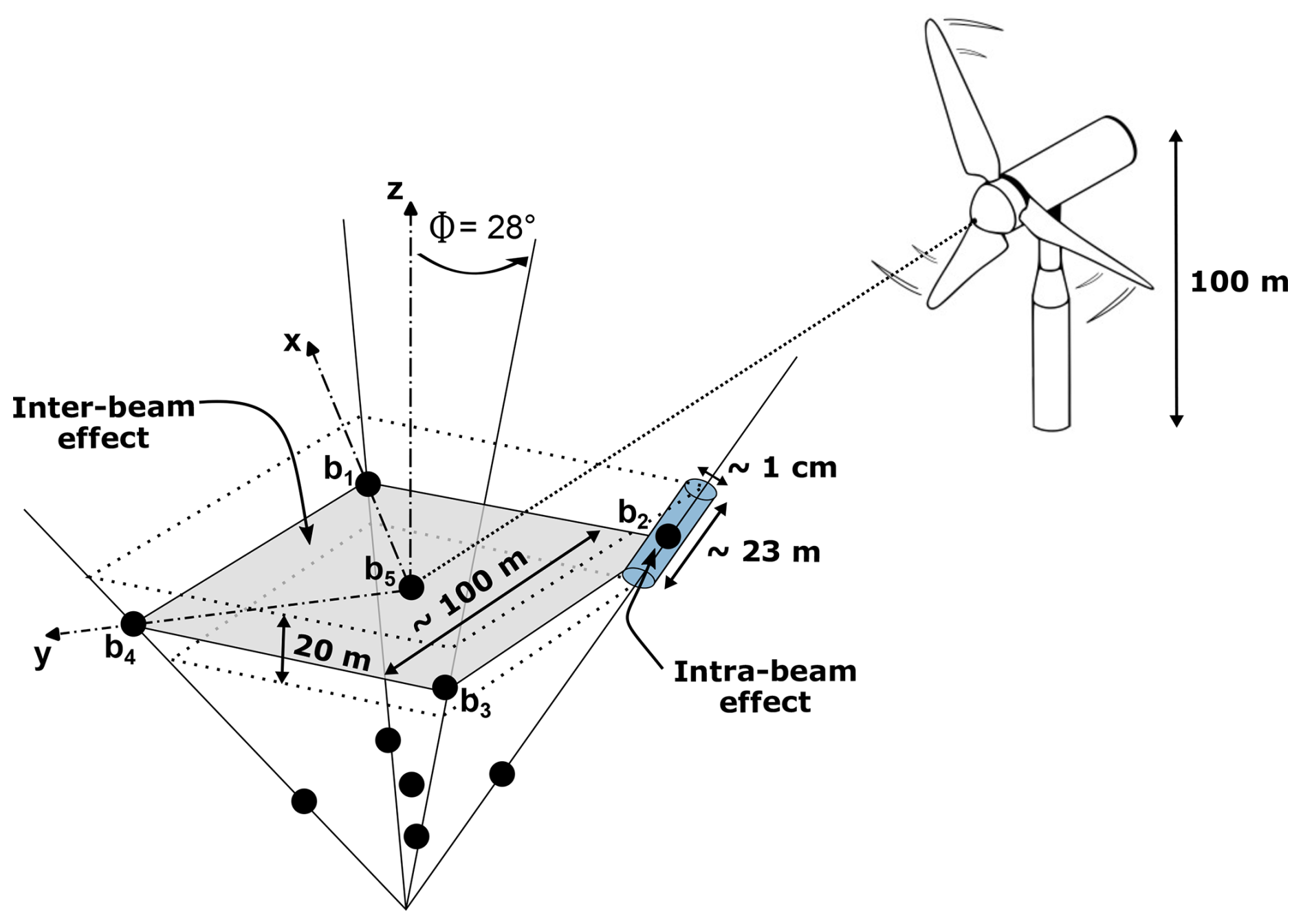
Figure 1 A schematic illustration of inter- and intra-beam effects in the WindCube v2.1 lidar profiler measurement process. The blue cylinder represents the probe volume, corresponding to the dimensions of the commercial lidar configuration. The positions of the five beams are labeled b_i, where i ranges from 1 to 5. The inclination of the diverging beams (from beam 1 to beam 4) with respect to the vertical z axis is ϕ=28°. Beam 5 is aligned with the z axis, while beams 1 and 3 are aligned with the x axis, and beams 2 and 4 are aligned with the y axis in the coordinate system of the instrument, as stipulated by the manufacturer. The black dots indicate the centers of the probe measurement volumes.

In the wind energy sector, the utilization of wind lidar profiler technology has gained significant traction in recent years, complementing the traditional meteorological mast equipped with in situ sensors like cup or sonic anemometers as the standard means of measuring key mean wind properties, such as speed and direction. Wind lidar profilers present compelling advantages, including the potential for cost reduction compared to meteorological masts and the capacity to measure at similar or even greater heights above the ground (e.g., Gottschall et al., 2012).

Wind lidar profilers can be categorized according to their emission waveforms, i.e., pulsed or continuous, and measuring technique, i.e., Doppler beam swinging (DBS) (Strauch et al., 1984) or velocity-azimuth display (VAD) (Browning and Wexler, 1968). The measurement methods used by wind lidar profilers are fundamentally different from those used by cup or sonic anemometers. Anemometers estimate wind speed over a small volume of just a few cubic centimeters, whereas pulsed lidar profilers provide an average over a cylindrical probe several dozen meters long with a cross-sectional diameter of less than 1 cm (Fig. 1).

However, wind lidar profilers have yet to garner widespread acceptance for turbulence measurement, which remains a focal point of ongoing research. In contrast to turbulence data derived from reference instruments such as sonic anemometers, turbulence data from lidar profiler measurements suffer from systematic errors induced by (i) the inter-beam effect, also known as the cross-contamination effect; (ii) the intra-beam effect, i.e., the space–time averaging effect within the probe volume (Fig. 1); and (iii) instrumental noise.

The inter-beam effect can result in either underestimation or overestimation of turbulence metrics, which arise from the modulation of energy associated with eddies of specific wavenumbers (Kelberlau and Mann, 2020). This effect is particularly relevant in the context of the assumption of instantaneous homogeneity, which underlies multi-beam lidar measurement techniques. Under this assumption, the turbulent field is considered spatially homogeneous across the beams at each instant in time, a condition that, if violated, can lead to inter-beam contamination. Any phase difference between the horizontal and vertical components of an eddy significantly impacts the filtering of flow structures, potentially leading to amplification or attenuation of their measured turbulent energy (Theriault, 1986; Gargett et al., 2009).

The intra-beam effect refers to a probe time-averaging phenomenon occurring within the lidar probe, leading to an underestimation of turbulence metrics. It arises from two anisotropic filtering processes: (1) spatial filtering due to averaging over the probe volume and (2) temporal filtering caused by averaging over the beam’s pulse accumulation time, Δt, at a given measurement position. These two effects give rise to a transfer function, H, applied by the instrument to the signal measured within the probe. The transfer function includes a part due to time-averaging (the sinc function) and a part due to space-averaging (the Gaussian function), such that

$$\begin{array}{}\text{(1)}& \begin{array}{rl}\left|H{|}^{\mathrm{2}}\right(\mathit{k})& ={\mathrm{sinc}}^{\mathrm{2}}\left({\displaystyle \frac{\mathrm{\Delta }t}{\mathrm{2}}}\mathit{k}\cdot \mathit{U}\right)\exp \left(-\left[{\mathit{\sigma }}_l^{\mathrm{2}}{\left(\mathit{k}\cdot \mathit{b}\right)}^{\mathrm{2}}\right.\right.\\ & \left.\left.+{\mathit{\sigma }}_r^{\mathrm{2}}\left(\parallel \mathit{k}{\parallel }^{\mathrm{2}}-(\mathit{k}\cdot \mathit{b}{)}^{\mathrm{2}}\right)\right]\right).\end{array}\end{array}$$

Here, k is the turbulent structure wave vector; b is the beam pointing vector; U is the vector associated with the wind direction of magnitude U; and σ_l and σ_r represent the Gaussian weighting factors in the along-beam and cross-beam directions, respectively. A detailed mathematical derivation of Eq. (1) is provided in the Supplement.

From Eq. (1), it follows that wind field structures with wavelengths smaller than σ_l in the along-beam direction are attenuated, as are those with wavelengths smaller than σ_r in the cross-beam direction. However, in the latter case, these structures are so small that the filtering effect becomes negligible, as the cross-section of the probe is approximately 1 cm (Fig. 1). Ultimately, assuming the Taylor frozen-turbulence hypothesis, the wave vector domain that passes through the filter is defined by the intersection of two slices: one perpendicular to the direction of U, which preserves structures longer than πΔtU, and another perpendicular to the direction of b, which retains structures longer than σ_l. All other structures are filtered out.

Pulsed lidar profilers require several seconds to complete a full scanning cycle, resulting in a low sampling rate that causes discrepancies between turbulence measurements taken by anemometers and those by lidar profilers (e.g., Peña et al., 2009). While the sampling rate governs how quickly the lidar progresses through a scan cycle, it is directly influenced by pulse accumulation time. Consequently, even if the sampling rate is increased, pulse accumulation can still limit the ability of the lidar to resolve small-scale turbulent structures. Since turbulent motion scales vary from milliseconds to hours and from centimeters to kilometers (e.g., Stull, 2000), it is crucial to account for both temporal and spatial filtering effects when assessing lidar-based turbulence measurements.

The concept of measuring turbulence using remote sensing instruments has gradually evolved since the early works in radar meteorology by Lhermitte (1962) and Browning and Wexler (1968). Lhermitte (1969) was the first to propose a method for inferring turbulence by analyzing the variance of radial velocity measurements through VAD scanning. Following this, Wilson (1970) conducted pioneering experiments using a pulsed Doppler radar to detect turbulence within the convective boundary layer (0.1–1.3 km). However, these early measurements were limited to turbulence scales larger than the pulse volume and smaller than the scanning circle, and no validation against reference instruments was performed, which calls their reliability into question.

Kropfli (1986) expanded Wilson's approach to capture turbulence scales larger than the scanning circle by integrating data from multiple scans. Although initially developed for Doppler radar, these methods were later adapted for Doppler lidar. Eberhard et al. (1989) were the first to apply Wilson’s and Kropfli's methods using lidar, and Gal-Chen et al. (1992) further refined the technique with a different scanning configuration. Despite these advancements, the significant probe length (around 100 m) limited studies to the convective boundary layer due to considerable probe volume averaging, especially near the ground. Frehlich (1994) and Frehlich et al. (1994) demonstrated the averaging effect of the measurement of the structure function, showing that this effect becomes more pronounced at smaller separation distances. To address this limitation, research shifted toward understanding and mitigating probe volume averaging effects. Smalikho et al. (2005) provided explicit formulae to account for the small-scale filtering effect of the finite probe volume in continuous-wave lidar, proposing three different methods for a staring lidar using (1) the width of the Doppler spectrum, (2) the velocity structure function, and (3) the 1D velocity spectrum. The expression for the structure function was derived under the assumption of local isotropy in the inertial subrange. Kristensen et al. (2011) later re-derived this expression, assuming a Lorentzian probe volume weighting function. However, averaging effects continue to pose challenges for turbulence measurements in the surface layer, where wind turbines operate. These effects lead to an underestimation of the variance derived from wind lidar compared to reference turbulence measurements, as demonstrated in Mann et al. (e.g., 2009) or Sjöholm et al. (e.g., 2009).

This paper explores advancements in the Vaisala WindCube v2.1 lidar profiler, focusing on a key modification: increasing the sampling rate by reducing the pulse accumulation time. This enhancement is assessed for its impact on measuring mean wind speed, data availability, and along-wind variance and its square root, i.e., the standard deviation. The latter is particularly important, as it is used in the wind power industry to compute turbulence intensity (TI), a critical metric for turbine load assessment, site suitability, and energy yield predictions. Additionally, the influence of instrumental noise is analyzed to confirm that the potential improvements in turbulence estimates with the higher sampling rate are not simply a result of increased noise.

The paper begins with a detailed overview of the data and methods, including the prototype configuration of the WindCube v2.1 and the field measurement setup (Sect. 2). The study compares the prototype configuration to the commercial WindCube v2.1 and to a sonic anemometer installed on a meteorological mast, which serves as the reference measurement. The methodology section then focuses on velocity spectra analysis, instrumental noise evaluation, and variance computation of instrument coordinates. Additionally, key performance indicators and error statistics used for validation are outlined. The results section presents findings on mean wind speed, data availability, standard deviation, variance, and instrumental noise contributions (Sect. 3). This is followed by a discussion of the implications, addressing both the advantages and challenges of a higher sampling rate (Sect. 4). The paper concludes with key takeaways on how the increased sampling rate enhances turbulence detection, while considering measurement limitations and filtering effects (Sect. 5).

2 Data and methods

2.1 Prototype configuration with increased sampling rate

The WindCube v2.1 lidar is designed for general atmospheric measurements, such as mean wind speed and direction, requiring a careful balance between the temporal resolution, spatial resolution, and carrier-to-noise ratio (CNR). Its default sampling rate is optimized to ensure high data quality and availability across varying altitudes and atmospheric conditions while maintaining system efficiency and manageable data processing.

The WindCube v2.1 employs the Doppler beam swinging (DBS) technique to measure wind speed. This method utilizes an optical switch that sequentially directs the lidar beam toward four directions (0, 90, 180, and 270° relative to the reference x axis), each inclined at ϕ=28° from the vertical. A fifth beam is directed vertically upwards, resulting in wind measurements at five distinct positions (Figs. 1 and 2).

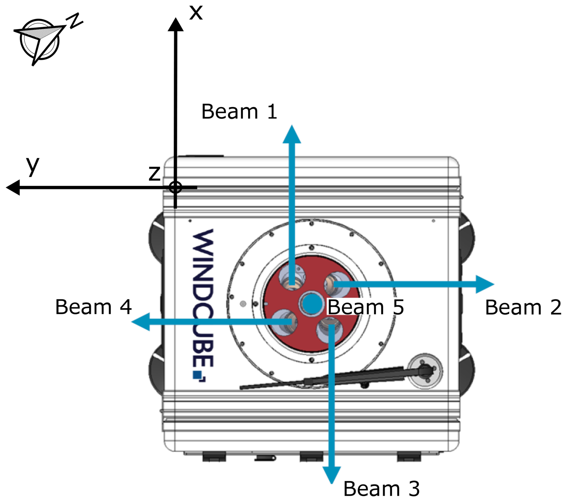
Figure 2 Top view of a WindCube v2.1 lidar showing the positions of its five beams. The x axis is oriented from beam 3 towards beam 1, the y axis extends from beam 4 towards beam 2, and the vertical z axis points upward along beam 5. The arrow indicates north. For the present study, the primary x axis of the lidars was oriented at −62° relative to north.

In its standard commercial configuration, the WindCube lidar collects data at each position for approximately Δt=0.8 s before switching to the next. Including transition times, a complete DBS scan is performed in 4 s, yielding a line-of-sight (LOS) velocity sampling rate of 0.25 Hz (Table 1). This sampling rate is well-suited for capturing turbulent structures larger than 100 m. However, wind turbine components experience loads from turbulence across a wide range of scales. Increasing the sampling rate is crucial for broadening the velocity spectrum captured by the lidar, potentially enabling the detection of extra turbulent energy that influences turbine performance.

Table 1 LOS velocity measurement parameters for the commercial and prototype WindCube v2.1 configurations.

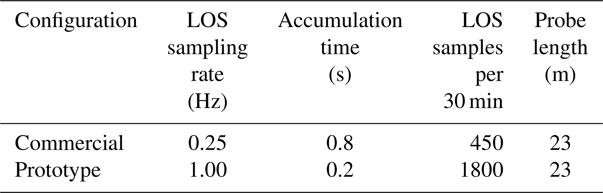
Theoretically, a higher sampling rate improves temporal resolution and extends the resolved turbulence frequency range. However, for wind lidar profiler technology, this enhancement comes with trade-offs. The duty cycle, which represents the proportion of time the lidar transmits pulses, decreases as the sampling rate increases, potentially reducing signal strength. Moreover, increasing the sampling rate requires a reduction in accumulation time, resulting in fewer pulses per sample and increasing noise. The commercial WindCube v2.1 configuration balances these factors to maximize data reliability. It integrates a high number of pulses per measurement to enhance signal quality, making it well-suited for general wind resource assessment. However, its probe length of approximately L_probe=23 m (Fig. 1, Table 1) limits its ability to resolve small eddies compared to point sensors like sonic anemometers.

In response to the demand for capturing additional turbulent energy, we developed a modified version of the WindCube v2.1 that operates 4 times faster, achieving a LOS velocity sampling rate of 1 Hz. This modification was achieved by reducing the accumulation time for data collection from each beam in conjunction with a reduction in the number of transmitted pulses. The factor of 4 was chosen as a compromise between increasing temporal resolution and maintaining an acceptable CNR and data availability. This choice is intended to keep wind measurements comparable to those from the commercial configuration, while enabling the capture of additional turbulent energy. The actual impact on measurement performance will be assessed in the study.

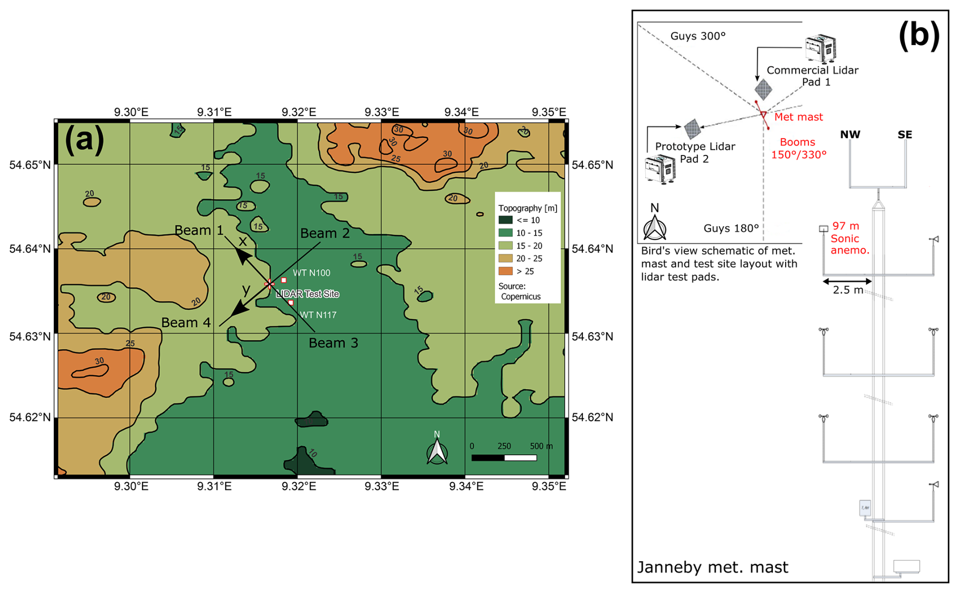
Figure 3 (a) Test site location at Janneby, Germany. Black arrows indicate the beam orientations for the commercial and prototype configurations. The x and y axes of the instrument coordinate system (see Fig. 2) are marked with black arrows. (b) Configuration of the meteorological mast, showing the position of the sonic anemometer. NW and SE denote the northwest and southeast directions. The schematic in panel (b) also provides a bird's-eye view of the meteorological mast and test site layout, including the lidar test pads.

2.2 Field measurement

The field measurement campaign was conducted by Det Norske Veritas (DNV) at the lidar validation test site in Janneby, Germany (Fig. 3). The site’s flat terrain ensures orography-free flow, making it ideal for lidar verification trials. It offers good exposure to largely undisturbed wind conditions from most directions. Situated just a few meters above mean sea level, the site features low surface roughness due to its predominantly agricultural land use (Fig. 3a). Two wind turbines (WT N100 and WT N117; Fig. 3a) are located near the meteorological mast. Their wake-affected wind sectors are shown in blue in Fig. 4 and lie outside the sectors selected for turbulence analysis (gray areas in Fig. 4, Sect. 2.5). The closest turbine is 210 m from the mast. A few small human-made structures (e.g., houses, sheds), all under 15 m in height, are situated about 500 m southwest of the mast.

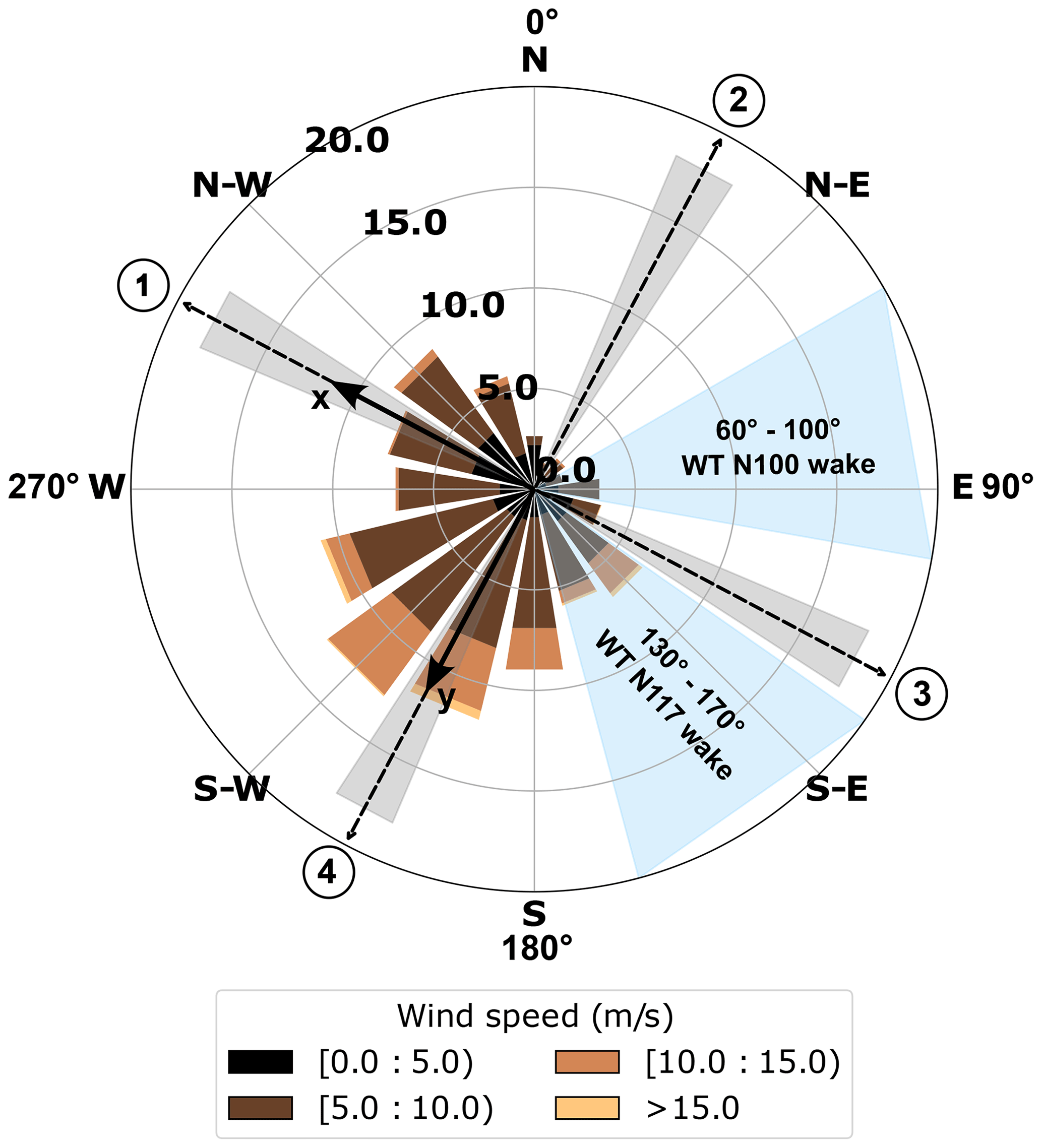
Figure 4 Wind rose showing wind data recorded over 47 d by the sonic anemometer at 97 m a.g.l. (meters above ground level). Gray-shaded areas indicate the wind sectors selected for the turbulence analysis in this study, corresponding to events when the wind was aligned (±5°) with either beam pair 1–3 (aligned with the x axis) or beam pair 2–4 (aligned with the y axis), as numbered in circles. Blue-shaded areas indicate wind sectors contaminated by the nearby wind turbines WT N100 and WT N117 (Fig. 3a).

The meteorological mast is a 100 m, 3-fold guyed lattice tower with a constant face width of 0.4 m. It is equipped with six MEASNET-calibrated Thies First Class Advanced cup anemometers (no. 4.3352) and a Thies 2D sonic anemometer (no. 4.3830). However, only the Thies 2D sonic anemometer is used in this study to provide reference measurements of mean wind speed and turbulence, as the cup anemometer data are not available. The mounting arrangements are consistent with the currently valid International Electrotechnical Commission (IEC) and International Energy Agency (IEA) recommendations for the use of anemometry at meteorological masts. As shown in Fig. 3b, the sonic anemometer points towards 150° from true north and is mounted at 97 m above ground, which corresponds to the average hub height of modern land-based wind turbines. The sonic anemometer was set to record continuous horizontal wind speed and direction at a sampling rate of 4 Hz. Potential wake effects from the meteorological mast structure were considered in the analysis of the sonic anemometer data. The wind directions associated with flow disturbances caused by the mast itself overlap with the wake sector of wind turbine WT N117, which was excluded from the analysis.

Adjacent to the measurement mast, both the commercial lidar configuration and a prototype version with an enhanced sampling rate were installed 3 and 13 m apart the mast, respectively. Both lidars were aligned such that beams 1 and 3, which correspond to the x axis (Fig. 2), were oriented at −62° from true north (Fig. 3). According to the manufacturer’s recommendation, the x axis is the primary axis and should be oriented relative to north. Beams 2 and 4 are fixed along the y axis. One of the measurement heights of both lidars was set to 97 m above ground to coincide with the height of the sonic anemometer deployment on the mast.

The field measurement campaign was conducted over two periods: from 12 to 25 November 2021 and from 7 December 2021 to 10 January 2022. These two measurement periods were combined to form a 47 d dataset. To facilitate a comparison of turbulence measurements, the sonic-derived wind dataset was resampled to match the sampling rate of the LOS velocities measured by the prototype configuration. This ensures that similar turbulence timescales are captured when calculating and comparing turbulence estimates. Therefore, the sonic anemometer measurements were resampled at 1 Hz.

The 47 d dataset was segmented into 2256 subsets, each comprising 30 min of data. For each subset, the commercial lidar provided 450 measurement points, while the prototype lidar provided 1800 points, corresponding to their respective sampling rates of 0.25 and 1 Hz (see Table 1). The selection of a 30 min window rather than the standard 10 min interval commonly used in the wind energy industry was guided by the aim of reducing random errors in turbulence measurements, following the recommendations of Lenschow et al. (1994).

2.3 Velocity spectra

The power spectral density of the velocity, i.e., the velocity spectra, provides valuable information about the distribution of turbulent kinetic energy across different scales of motion within the wind flow. This understanding helps in characterizing turbulence and its effects on wind turbine performance and structural loads.

Velocity spectra were computed using Welch's method (Welch, 1967). This method computes an estimate of the spectrum by dividing the data into overlapping segments, computing a modified periodogram for each segment, and averaging the periodograms. The Hann window with 50 % overlap was applied to each segment to reduce spectral leakage and improve frequency resolution. The 50 % overlap is a reasonable trade off between accurately estimating the signal power, while not over-counting any of the data.

Fitting turbulence velocity spectra derived from lidar-reconstructed velocity components to turbulence models should be avoided due to the inter-beam effect, which distorts the spectra and complicates their physical interpretation. Therefore, such spectra were not considered in this study. The focus was on velocity spectra S_i(f) derived from the LOS velocities measured by beam i. The primary limitation of this approach is the intra-beam effect. Spectra were computed for each 30 min subset of data.

The spectra, S_i(f), were fitted with a parametric expression (Teunissen, 1980; Olesen et al., 1984; Tieleman, 1995) in the frequency domain f, to which we add a component N_i associated with the power spectral density of instrumental noise of the LOS velocity measured by beam i (see Sect. 2.4):

$$\begin{array}{}\text{(2)}& S_i\left(f\right)={\displaystyle \frac{m}{(\mathrm{1}+nf{)}^{\mathit{\beta }}}}+N_i.\end{array}$$

The coefficient m primarily controls the vertical scaling or amplitude of the spectrum, whereas n influences the rate at which the function decays as f increases. The exponent β determined the shape of the spectrum.

Three different weighting schemes were considered: an unweighted scheme, a low-frequency-weighted scheme with weights proportional to the logarithm of the frequency, and a high-frequency-weighted scheme with weights inversely proportional to the logarithm of the frequency. Assessing the fitting accuracy included comparing the variance obtained from the integrated fitted spectra with the measured spectra and calculating their absolute relative differences.

2.4 Instrumental noise

Lidar measurements are inherently influenced by signal noise and potential variations in aerosol fall speeds, both of which contribute additional terms to the observed variance. Assuming that all atmospheric flow contributions to the observed LOS velocity variance within the short timescales considered are of a turbulent nature, the variance ${\mathit{\sigma }}_{{\mathrm{b}}_i}^{\mathrm{2}}$ of the LOS velocity measured by beam i can be expressed as the sum of three independent terms (Doviak and Zrnic, 1993):

$$\begin{array}{}\text{(3)}& {\mathit{\sigma }}_{{\mathrm{b}}_i}^{\mathrm{2}}={\mathit{\sigma }}_{{\mathrm{p}}_i}^{\mathrm{2}}+{\mathit{\sigma }}_{{\mathrm{n}}_i}^{\mathrm{2}}+{\mathit{\sigma }}_{{\mathrm{d}}_i}^{\mathrm{2}}.\end{array}$$

Here, ${\mathit{\sigma }}_{{\mathrm{p}}_i}^{\mathrm{2}}$ represents the net contribution from atmospheric turbulence at scales measurable by the lidar (Brugger et al., 2016), ${\mathit{\sigma }}_{{\mathrm{n}}_i}^{\mathrm{2}}$ denotes the variance associated with instrumental noise, and ${\mathit{\sigma }}_{{\mathrm{d}}_i}^{\mathrm{2}}$ accounts for the variance caused by variations in aerosol terminal fall speeds within the probe volume. However, ${\mathit{\sigma }}_{{\mathrm{d}}_i}^{\mathrm{2}}$ can typically be neglected, as particle fall speeds are generally less than 1 cm s⁻¹ (e.g., Bodini et al., 2018). Noise has been identified through two different methods: a spectral approach and an autocorrelation approach, as accurately identifying the variance of noise is critical to our study.

2.4.1 Spectral method

Instrumental noise is a critical factor in the spectral analysis of velocity time series. In the spectrum of a velocity time series, this noise typically manifests as a flattening of the spectrum at higher frequencies, indicating a white-noise characteristic that contributes equally across these frequencies (e.g., Thomson et al., 2012; Durgesh et al., 2014; Guerra and Thomson, 2017; McMillan and Hay, 2017; Thiébaut et al., 2020). At lower frequencies, the spectrum is usually dominated by the actual signal, which may show a characteristic decay or specific features related to the physical process being measured, such as turbulence. As the frequency increases, the influence of the instrumental noise becomes more prominent, leading to a flattened spectral region where the noise dominates.

In Eq. (2), N_i represents the constant power spectral density of noise, which contributes to the spectral flattening observed at higher frequencies. The variance of the noise depends on the technical characteristics of the device measuring the velocity, such as the Nyquist velocity, the signal spectral width, the number of pulses and points per range gate, and the signal-to-noise ratio. Theoretical expressions for the variance of this noise can be derived and subsequently removed from the computed turbulence metrics to improve accuracy (Pearson et al., 2009; O'Connor et al., 2010; Bodini et al., 2018, 2019; Wildmann et al., 2019). However, the technical specifications of lidar profilers are no longer openly shared with users, making it impossible to evaluate this noise theoretically. To address this, it is essential to evaluate the noise using an alternative method, such as the spectral approach employed in this study. This approach is comparable to the method proposed by Richard et al. (e.g., 2013) or Durgesh et al. (e.g., 2014). It enables the determination of the power spectral density of noise, N_i, associated with the LOS velocity measured by beam i. Subsequently, the variance of the instrumental noise, ${\mathit{\sigma }}_{{\mathrm{n}}_i}^{\mathrm{2}}$, can be derived by multiplying N_i by the Nyquist frequency, f_N (e.g., McMillan and Hay, 2017):

$$\begin{array}{}\text{(4)}& {\mathit{\sigma }}_{{\mathrm{n}}_i}^{\mathrm{2}}=N_i{f}_{\mathrm{N}}.\end{array}$$

2.4.2 Autocorrelation function method

An alternative method for computing the variance of the instrumental noise involves the calculation of the autocorrelation function (ACF) of the squared LOS velocity time series, as proposed by Lenschow et al. (2000). The ACF quantifies the similarity between a signal and its time-shifted versions across various time lags. This measure provides insight into how much of the signal correlates with its past values, which is essential for distinguishing between the noise and signal components.

According to Lenschow et al. (2000), after calculating the ACF, the ACF values (excluding the first lag) are fitted to a $\mathrm{2}/\mathrm{3}$ power-law function. This power-law model describes the decay of correlation over time, allowing for the extraction of a coefficient that characterizes how the correlation diminishes as the time lag increases. From this power-law fit, the value of the ACF as the lag tends toward zero is estimated by extrapolation from the fitted model. This value is associated with the signal variance.

Subsequently, the total variance of the signal is calculated. The instrumental noise variance, ${\mathit{\sigma }}_{{\mathrm{n}}_i}^{\mathrm{2}}$, is then determined by subtracting the signal variance derived from the fitted power-law model from the total variance. This process enables the separation of the signal and noise contributions from the overall variance. The application of the ACF method requires that the data be stationary. To verify this assumption, a stationarity test was performed for each 30 min subset using the augmented Dickey–Fuller (ADF) test. The null hypothesis of the ADF test states that the data are non-stationary, which was assessed through the determination of a significance level, commonly set to 0.05 or 5 % (e.g., Hayat, 2010).

2.5 Computation of the variance in instrument coordinates

The conventional method for computing variance and standard deviation (the square root of variance) from wind lidar profiler measurements relies on deriving second-order statistics from the reconstructed instantaneous velocity components based on LOS velocities. This approach inherently combines, at each time step, measurements taken at sampling points separated by several tens of meters, depending on the height level of interest. The assumption of instantaneous flow homogeneity (inter-beam effect) introduces uncertainty into the derived statistics, which is difficult to quantify and can lead to either overestimation or underestimation of the standard deviation, depending on the frequency and flow configuration. Additionally, this traditional method is affected by both intra-beam filtering and instrumental noise. Crucially, because variance is computed from the reconstructed instantaneous velocity components, it does not account for the noise-induced variance present in the LOS velocity time series, which will result in overestimation of variance.

The combined influence of the inter-beam effect, intra-beam effect, and instrumental noise can result in variance estimates derived from the traditional approach that may appear to align more closely with those derived from a sonic anemometer but for reasons unrelated to the actual turbulence characteristics. Consequently, the benefits of an increased sampling rate for turbulence measurement using a lidar profiler cannot be accurately assessed with this approach.

The variance method, as referred to in the studies (e.g., Stacey et al., 1999a, b; Lu and Lueck, 1999; Rippeth et al., 2002; Guerra and Thomson, 2017; Thiébaut et al., 2022), offers an alternative to the traditional approach for computing variance. This method calculates the second-order statistics of the three velocity components by deriving them directly from the second-order statistics of the LOS velocities. Unlike the traditional approach, the variance method is unaffected by the inter-beam effect. However, it is still influenced by the intra-beam effect and instrumental noise. Notably, the impact of instrumental noise can be identified and removed. Hereafter, hat notation is used to denote the standard deviation or variance derived from this method.

The variance method enables the calculation of the variances, ${\widehat{\mathit{\sigma }}}_x^{\mathrm{2}}$ and ${\widehat{\mathit{\sigma }}}_y^{\mathrm{2}}$, of the velocity components u_x and u_y (in instrument coordinates) as

$$\begin{array}{}\text{(5)}& {\displaystyle }& {\displaystyle }{\widehat{\mathit{\sigma }}}_x^{\mathrm{2}}={\displaystyle \frac{\mathrm{1}}{\mathrm{2}{\sin }^{\mathrm{2}}\mathit{\varphi }}}\left({\mathit{\sigma }}_{{\mathrm{p}}_{\mathrm{3}}}^{\mathrm{2}}+{\mathit{\sigma }}_{{\mathrm{p}}_{\mathrm{1}}}^{\mathrm{2}}-\mathrm{2}{\cos }^{\mathrm{2}}\mathit{\varphi }{\mathit{\sigma }}_{{\mathrm{p}}_{\mathrm{5}}}^{\mathrm{2}}\right)\text{(6)}& {\displaystyle }& {\displaystyle }{\widehat{\mathit{\sigma }}}_y^{\mathrm{2}}={\displaystyle \frac{\mathrm{1}}{\mathrm{2}{\sin }^{\mathrm{2}}\mathit{\varphi }}}\left({\mathit{\sigma }}_{{\mathrm{p}}_{\mathrm{2}}}^{\mathrm{2}}+{\mathit{\sigma }}_{{\mathrm{p}}_{\mathrm{4}}}^{\mathrm{2}}-\mathrm{2}{\cos }^{\mathrm{2}}\mathit{\varphi }{\mathit{\sigma }}_{{\mathrm{p}}_{\mathrm{5}}}^{\mathrm{2}}\right),\end{array}$$

where ${\mathit{\sigma }}_{{\mathrm{p}}_i}^{\mathrm{2}}={\mathit{\sigma }}_{{\mathrm{b}}_i}^{\mathrm{2}}-{\mathit{\sigma }}_{{\mathrm{n}}_i}^{\mathrm{2}}$ (Eq. 3) is the variance of the LOS velocity recorded by beam i, corrected for the variance of instrumental noise.

In this paper, we restrict the application of the variance method to situations where the wind aligns (±5°) with a single pair of opposite beams (either pair 1–3 or pair 2–4) of the lidar profilers. This alignment condition was met in 17.1 % of the cases (gray areas in Fig. 4). Under these conditions, it can be reasonably assumed that the covariance term, ${\widehat{\mathit{\sigma }}}_{uv}$ (where v represents the cross-wind velocity), which corresponds to ${\widehat{\mathit{\sigma }}}_{xy}$ in this specific condition, is negligible (e.g., Newman et al., 2016). Specifically, when the wind aligns with beams 1 and 3, we have ${\widehat{\mathit{\sigma }}}_u^{\mathrm{2}}={\widehat{\mathit{\sigma }}}_x^{\mathrm{2}}$. Conversely, when the wind aligns with beams 2 and 4, it follows that ${\widehat{\mathit{\sigma }}}_u^{\mathrm{2}}={\widehat{\mathit{\sigma }}}_y^{\mathrm{2}}$. For brevity, we use ${\widehat{\mathit{\sigma }}}^{\mathrm{2}}$ in the place of ${\widehat{\mathit{\sigma }}}_u^{\mathrm{2}}$ hereafter. The standard deviation, $\widehat{\mathit{\sigma }}$, is then compared to the along-wind standard deviation, σ, which is derived from sonic anemometer measurements.

2.6 Key performance indicators and acceptance criteria

The first step of our analysis focuses on key performance indicators (KPIs) related to mean wind statistics, such as wind speed. These include the mean differences, slope, and the coefficient of determination (R²) at reference heights corresponding to sonic anemometer measurements. The verification process follows the standard lidar performance requirements set by DNV (2009), which define acceptance criteria (ACs) as either best practice or minimum-allowable tolerances. Applied to wind speed, these criteria flag any KPIs exceeding the defined thresholds as deviations. Table 2 summarizes the ACs established by DNV, which are tested in this paper for wind speed KPIs.

Table 2 Acceptance criteria for KPIs of mean wind speed in wind lidar profiler certification.

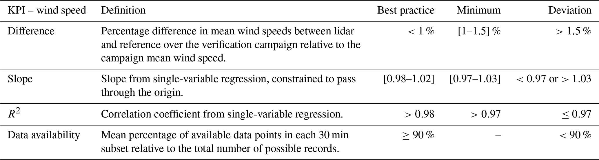
Additionally, the paper addresses data availability. Data availability is defined as the ratio of valid data points returned by the lidar to the maximum number of possible points that could be acquired during the test. To pass the test, the standard lidar performance set the data availability threshold to 90 % (Table 2).

2.7 Error statistics metrics

This paper focuses on turbulence measurements, specifically the standard deviation and variance of the along-wind velocity, obtained from both the commercial and prototype lidars. These measurements are compared to the standard deviation provided by the reference instrument: the sonic anemometer. To assess the accuracy and reliability of the lidar turbulence measurements, various error statistics are used. These include the following:

• Root-mean-square error (RMSE). This quantifies the average magnitude of the errors.

  $$\begin{array}{}\text{(7)}& \mathrm{RMSE}=\sqrt{{\displaystyle \frac{\mathrm{1}}{M}}\sum _{i=\mathrm{1}}^M{\left(X_i-Y_i\right)}^{\mathrm{2}}}\end{array}$$

• Mean absolute error (MAE). This calculates the average absolute difference between predicted and observed values.

  $$\begin{array}{}\text{(8)}& \mathrm{MAE}={\displaystyle \frac{\mathrm{1}}{M}}\sum _{i=\mathrm{1}}^M|X_i-Y_i|\end{array}$$

• Bias. This represents the systematic error between the lidar and reference measurements.

  $$\begin{array}{}\text{(9)}& \mathrm{Bias}={\displaystyle \frac{\mathrm{1}}{M}}\sum _{i=\mathrm{1}}^M\left(X_i-Y_i\right)\end{array}$$

• Coefficient of determination (R²). This indicates the proportion of variance in the lidar measurements that is explained by the reference data.

  $$\begin{array}{}\text{(10)}& R^{\mathrm{2}}=\mathrm{1}-{\displaystyle \frac{\sum _{i=\mathrm{1}}^M{\left(X_i-Y_i\right)}^{\mathrm{2}}}{\sum _{i=\mathrm{1}}^n{\left(Y_i-\stackrel{\mathrm{‾}}{Y}\right)}^{\mathrm{2}}}}\end{array}$$

Here, X_i represents the lidar measurement, Y_i the corresponding reference measurement from the sonic anemometer, $\stackrel{\mathrm{‾}}{Y}$ the mean of the reference measurements, and M the number of turbulence estimates. Together, these statistical metrics provide a comprehensive evaluation of the lidar's performance at capturing turbulence characteristics relative to the reference instrument.

3 Results

3.1 Mean wind speed and data availability

The first step in proposing enhancements to lidar technology is to evaluate their impact on mean wind speed measurements. Figure 5a shows that the mean vertical wind speed profiles measured by both configurations are closely aligned. However, the difference between the mean wind speed measurements provided by the commercial configuration and the reference measurement (black cross in Fig. 5) at the reference altitude is smaller, amounting to 0.98 % compared to a 1.41 % difference for the prototype configuration. These results demonstrate that the commercial configuration closely matches the best-practice AC criterion for the difference in mean wind speed, while the prototype configuration, with a larger difference, only meets the minimum criterion (Tables 2 and 3).

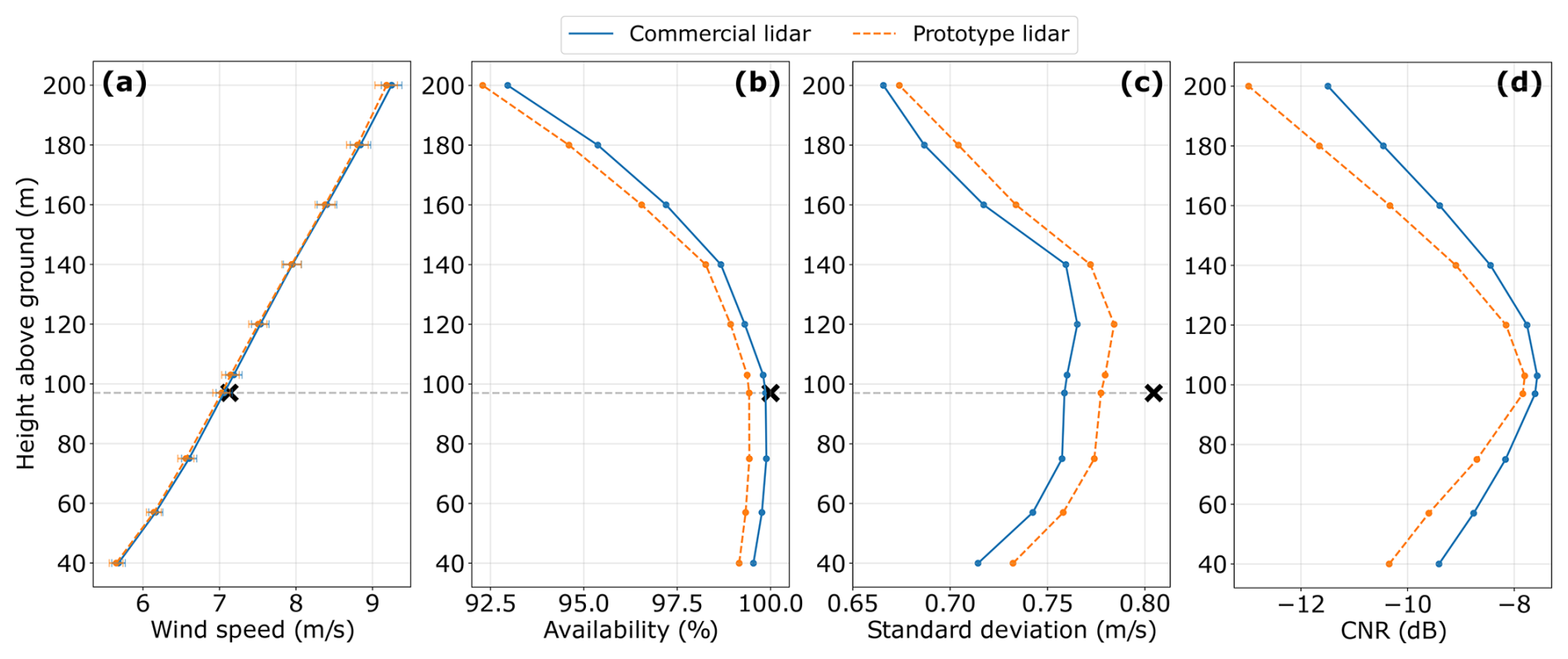
Figure 5 Mean vertical profiles, averaged across the 47 d dataset, of wind speed (a), data availability (b), the standard deviation derived from the variance method (c), and CNR (d) measured using the commercial (solid-blue curves) and prototype (dashed-orange curves) configurations. In panel (a), the error bars represent 95 % confidence intervals computed via bootstrapping, illustrating the statistical uncertainty in the mean. The black crosses represent the reference measurements from the sonic anemometer, and the gray dashed horizontal line marks its position at 97 m above ground.

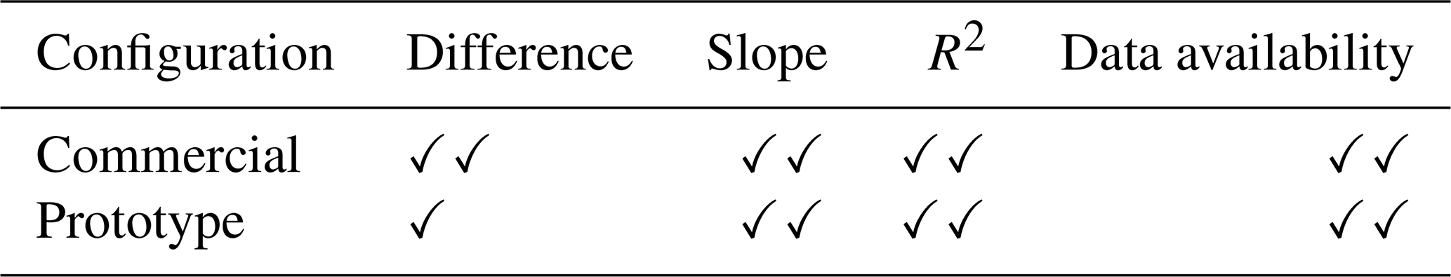
Table 3 Acceptance criteria for KPI achievement applied to the mean wind speed associated with the commercial and prototype configurations. ✓✓ denotes the best practice and ✓ indicates the minimum acceptance, as defined in Table 2.

Moreover, the commercial configuration exhibits data availability ranging from 99.5 % at the lowest measurement height, i.e., 40 m above the ground, to 93.0 % at the highest, i.e., 200 m above the ground, with an overall vertical average availability of 98.2 % (Fig. 5b). Similarly, the prototype configuration follows this trend, with data availability decreasing with altitude. The prototype achieves a vertical average availability of 97.7 %, with a minimum of 92.3 % recorded at the highest measurement altitude. The prototype configuration consistently shows data availability that is, on average, 0.5 % lower than that of the commercial configuration at nearly all measurement altitudes. Both lidar configurations exceed the 90 % data availability threshold set by DNV (2009).

Figure 6 presents the linear regression of the 30 min averaged wind speed measured by both lidar configurations in comparison to the reference instrument. Both the commercial and prototype configurations match the best-practice criteria, with slope values of 1.0 and R² values of 0.9847 for the commercial configuration. The prototype configuration shows values that are 1 % lower for the slope and similar R², but these differences are minimal and are still within the acceptable range for best practice.

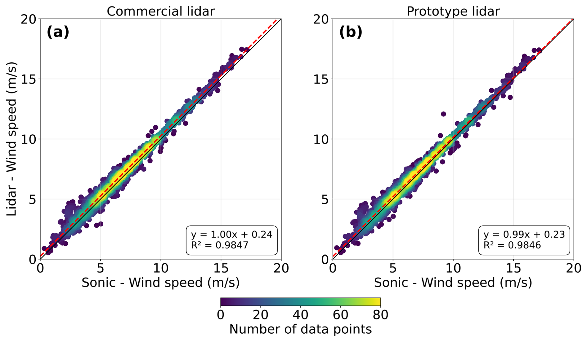
Figure 6 Scatter plots of the 30 min averaged wind speed measurements over the 47 d campaign, comparing the commercial lidar (a) and prototype lidar (b) with the reference sonic anemometer. Red-dashed lines indicate the linear regression fits.

3.2 Impact of the sampling rate on turbulence energy capture

The impact of increasing the sampling rate on turbulence measurement can initially be assessed using data from a sonic anemometer, specifically through the computation of along-wind velocity spectra. Integrating these spectra provides the along-wind variance, σ². Figure 7 illustrates the individual spectra and the mean spectrum averaged over the 47 d dataset in both log–log and linear formats. The mean spectrum clearly follows the $f^{-\mathrm{5}/\mathrm{3}}$ slope, confirming the presence of the energy cascade (Fig. 7a).

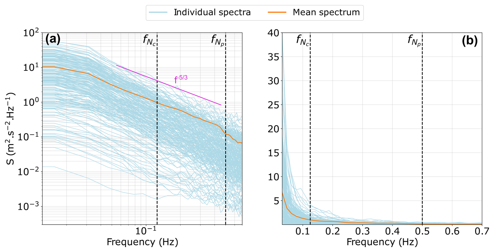
Figure 7 Individual spectra (light-blue curves) and the mean spectrum (orange curve) measured by the sonic anemometer over the 47 d measurement campaign presented in log–log (a) and linear (b) formats. Vertical black-dashed lines indicate the Nyquist frequencies, $f_{{\mathrm{N}}_{\mathrm{c}}}$ and $f_{{\mathrm{N}}_{\mathrm{p}}}$, for the commercial and prototype lidar configurations, respectively. The solid-pink line in panel (a) shows the classic spectral slope $f^{-\mathrm{5}/\mathrm{3}}$.

The linear representation (Fig. 7b) highlights the fact that most of the energy associated with larger eddies is concentrated in the frequency range from 0 to $f_{{\mathrm{N}}_{\mathrm{c}}}=\mathrm{0.125}$ Hz, corresponding to the Nyquist frequency of the LOS velocity in the commercial lidar configuration. However, additional energy associated with smaller eddies exists within the range from $f_{{\mathrm{N}}_{\mathrm{c}}}$ to $f_{{\mathrm{N}}_{\mathrm{p}}}=\mathrm{0.5}$ Hz, the latter being the Nyquist frequency of the prototype lidar configuration.

To quantify this effect, the variance was computed by integrating the spectra over two frequency ranges. First, the integration from 0 to $f_{{\mathrm{N}}_{\mathrm{c}}}$ simulated the variance measurable by a sonic anemometer with a sampling rate equivalent to that of the commercial lidar. This yielded a mean variance of 0.4712 m² s⁻². Second, the integration from 0 to $f_{{\mathrm{N}}_{\mathrm{p}}}$ simulated the variance measurable with a sampling rate equivalent to that of the prototype lidar, resulting in a mean variance of 0.6314 m² s⁻². This comparison indicates that increasing the sampling rate by a factor of 4 relative to the commercial lidar configuration could capture an additional 34 % of the variance. However, this represents the maximum possible improvement, as it is derived from measurements using a sonic anemometer, which is not affected by technical limitations such as the space–time volume averaging inside the probe of a wind lidar profiler.

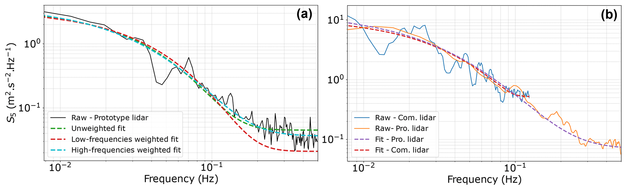
Figure 8 (a) The LOS velocity spectrum measured by beam 5 of the prototype lidar (solid black) and fitted using Eq. (2) with three different weighting schemes: unweighted (dashed green), low-frequency-weighted (dashed red), and high-frequency-weighted (dashed blue). This panel corresponds to the study focused on selecting the optimal weighting scheme. (b) The optimal scheme (high-frequency weighted) is applied to the LOS velocity spectrum measured by beam 5 of the commercial lidar (blue) and the prototype lidar (orange).

3.3 LOS velocity spectra

The determination of the instrumental noise from the spectral method involves computational fitting of the LOS velocity spectra using a parametric expression (Eq. 2). Three weighting schemes were systematically explored to enhance fitting accuracy and minimize errors relative to the measured spectra. Figure 8a illustrates an example of the three weighting schemes applied to a measured spectrum. This iterative process was conducted across both lidar configurations, yielding consistent results described hereafter.

The fitted spectra closely matched in the low-frequency domain, up to approximately f=0.1 Hz, but strong divergences were observed thereafter. The low-frequency-weighted scheme produced a curve substantially below the measured spectra at higher frequencies, whereas the unweighted scheme yielded a curve slightly above the measured spectra in this frequency range. In contrast, the high-frequency-weighted scheme provided a fit that closely matched the measured spectra across all frequencies and exhibited the lowest mean error. For instance, when applied to the prototype lidar, the mean variance was 0.2321 m² s⁻² for all integrated fitted spectra using the high-frequency-weighted scheme compared to 0.2262 m² s⁻² for all integrated measured spectra. This results in an absolute error of 2.6 %. Conversely, not employing any weighting during the fitting process resulted in an absolute error between the mean variance nearly 3 times higher, 8.5 %. Assigning weights to the low frequencies resulted in a mean absolute error exceeding 6 times that of the high-frequency-weighted scheme, 16.9 %. Thus, the high-frequency-weighted scheme was chosen for the fitting. An example of this fitting applied to individual LOS velocity spectra for both the commercial and prototype configurations is shown in Fig. 8b. This weighted scheme enabled the systematic identification of the plateau at higher frequencies, which is characteristic of white noise. Other weighting schemes did not consistently exhibit this plateau, making it challenging to reliably determine the value of N_i.

3.4 Instrumental noise

3.4.1 Carrier-to-noise ratio

Figure 5d shows that the CNR of the prototype lidar is consistently lower than that of the commercial system throughout the altitudes of measurement, with a mean value across all heights of −8.9 dB. On average, the prototype lidar's CNR is 8.5 % lower, indicating a weaker signal and thus a higher relative noise level compared to the commercial lidar. Despite this difference in magnitude, the mean vertical profiles of CNR for both lidars follow the same trend: the CNR reaches a minimum near the ground, increases to a maximum at approximately 100 m above ground, and then decreases again, reaching another minimum at the highest measurement altitude.

3.4.2 Comparison of the spectral and ACF methods

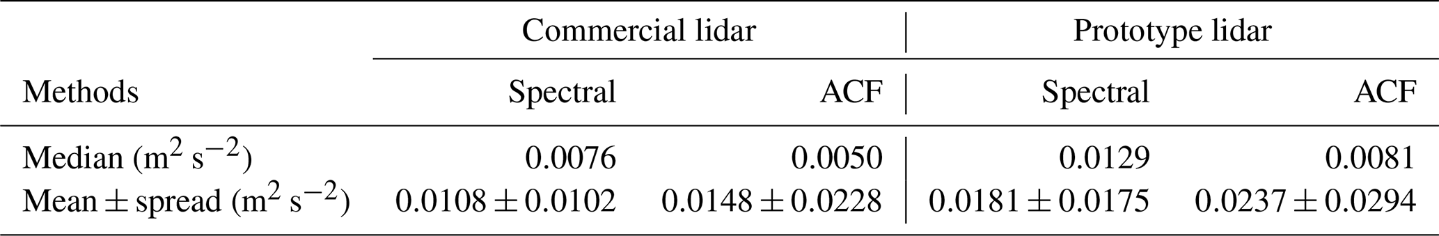
The spectral method yields a median variance that is 1.5 times higher than that of the ACF method for the commercial and prototype lidars (Table 4). While this suggests differences in how each method characterizes noise, the spectral method also results in a mean instrumental noise that is 30 %–40 % lower than that of the ACF method, indicating variations in the way noise is estimated. Moreover, the spread of mean values is notably narrower when using the spectral method, particularly for the commercial lidar, where it is reduced by half compared to in the ACF method. This suggests a potential advantage in terms of consistency and stability. Given these observations, we used the spectral method to correct the measured variance, as it appeared to provide more stable estimates of instrumental noise.

Table 4 Median and mean (± spread) variance of instrumental noise for commercial and prototype lidars computed from the LOS velocity measurements across all beams using the spectral and ACF methods.

To validate the applicability of the ACF method and investigate the higher spread of mean values of instrumental noise associated with this method, the ADF test was applied to each 30 min data subset. The results show that approximately 8 % of the subsets yielded p values just above the 0.05 significance threshold, although none exceeded 0.06. This indicates that, for these subsets, the null hypothesis of non-stationarity (see Sect. 2.4.2) could not be rejected. Consequently, they cannot be confidently considered stationary, and the ACF method is not strictly valid for them. This limitation may partly account for the higher variability in noise estimates produced by the ACF method, as non-stationary data can lead to inconsistent results in autocorrelation-based analyses.

3.4.3 Contribution of instrumental noise to the measured LOS velocity variances

The parametric expression (Eq. 2) used to fit the LOS velocity spectra measured by beam i enables the identification of the power spectral density of instrumental noise, N_i, and the derivation of the variances, ${\mathit{\sigma }}_{{\mathrm{n}}_i}^{\mathrm{2}}$ (Eq. 4). Figure 9 compares the mean magnitude of ${\mathit{\sigma }}_{{\mathrm{n}}_i}^{\mathrm{2}}$ to the mean variance of the net contribution from atmospheric turbulence, ${\mathit{\sigma }}_{{\mathrm{p}}_i}^{\mathrm{2}}$, corrected for the instrumental noise at scales observable by the commercial and prototype lidar profilers.

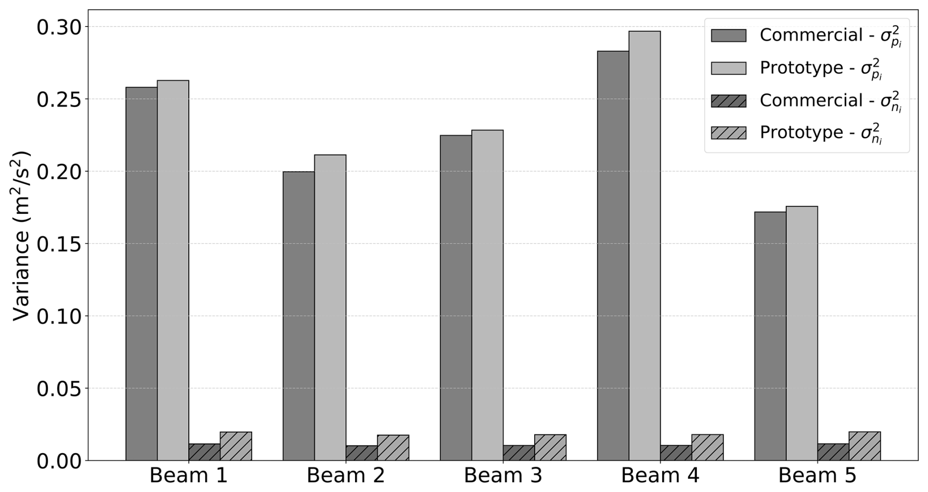
Figure 9 Mean variance of the net contribution from atmospheric turbulence (${\mathit{\sigma }}_{{\mathrm{p}}_i}^{\mathrm{2}}$) corrected for instrumental noise derived from the spectral method and measured by each beam i at scales observable by the commercial (dark-gray) and prototype (light-gray) lidar profilers. Dashed areas represent the mean variance of instrumental noise, ${\mathit{\sigma }}_{{\mathrm{n}}_i}^{\mathrm{2}}$. The averages were computed over the 47 d dataset.

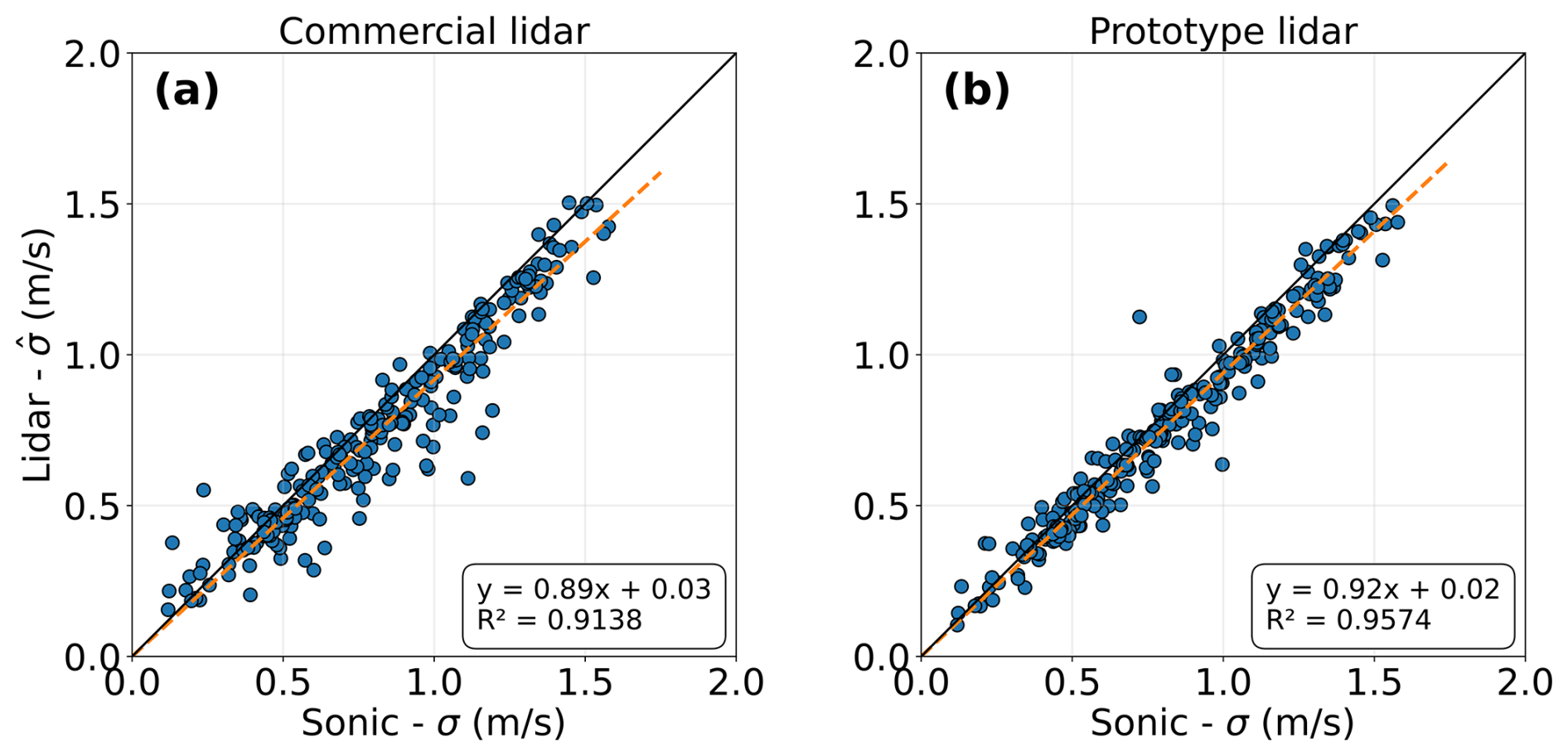
Figure 10 Scatter plots of the along-wind standard deviation, $\widehat{\mathit{\sigma }}$, derived from the variance method applied to measurements of the commercial and prototype lidar configurations versus the standard deviation, σ, derived from the reference sonic anemometer. The standard deviation estimates are restricted to cases where the wind direction was aligned with one pair of opposite beams.

The mean values of ${\mathit{\sigma }}_{{\mathrm{n}}_i}^{\mathrm{2}}$, which are nearly identical across all beams, were found to be 0.0108 m² s⁻² for the commercial configuration (Table 4). A similar trend was observed for the prototype configuration, although the mean variance of instrumental noise was 68 % higher, 0.0181 m² s⁻² (Table 4). Notably, the contribution of instrumental noise variance to the total variance, ${\mathit{\sigma }}_{{\mathrm{b}}_i}^{\mathrm{2}}$ (Eq. 3), was found to be 4.8 % and 7.4 % for the commercial and prototype lidar configurations, respectively.

The mean variances, ${\mathit{\sigma }}_{{\mathrm{p}}_i}^{\mathrm{2}}$ were consistently higher for measurements obtained with the prototype configuration. Across all beams, the mean value was 0.2288 m² s⁻², which is 7.8 % higher than the corresponding mean value for the commercial lidar measurements.

3.5 Along-wind standard deviation

Figure 10 presents scatter plots of the along-wind standard deviation, $\widehat{\mathit{\sigma }}$, derived from the variance method applied to measurements of both lidar configurations compared to the standard deviation, σ, obtained from the reference sonic anemometer. The prototype configuration demonstrates superior performance across all error metrics, with bias, MAE, and RMSE approximately 25 % lower than those of the commercial configuration (Table 5). Additionally, the coefficient of determination is 5 % higher. There is also a reduction in the relative error in the mean standard deviation, with the prototype configuration showing values of 5.7 % compared to 7.8 % for the commercial configuration.

Table 5 Error statistics of the along-wind standard deviation derived from the variance method corrected for instrumental noise and applied to measurements collected by the commercial and prototype lidars in comparison to the reference sonic anemometer.

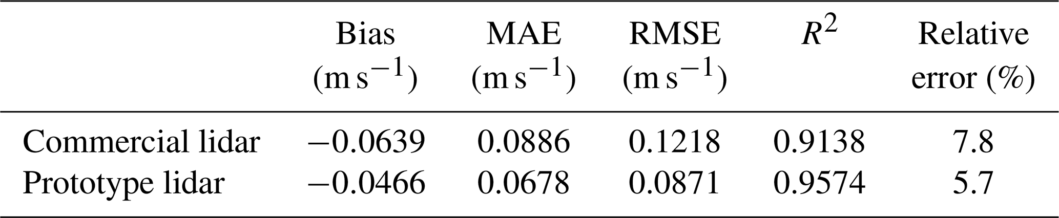
Figure 11 presents wind-speed-binned estimates of $\widehat{\mathit{\sigma }}$ compared to estimates of σ (black curve) as a function of binned-averaged wind speed. For all wind speeds, the standard deviation measured by the sonic anemometer consistently remains higher than that derived from both lidar configurations. Below wind speeds of 8 m s⁻¹, the standard deviation values from both lidar configurations closely match each other. Within this wind speed range, the standard deviation associated with the commercial lidar is 2.7 % higher than that from the prototype configuration. However, above this wind speed threshold, the standard deviation associated with the prototype configuration increases more rapidly with wind speed compared to the commercial lidar. In this wind speed range, the standard deviation associated with the prototype lidar is 13.0 % higher than that associated with the commercial configuration. For all wind speed ranges, the prototype lidar measurements exhibited a mean standard deviation and variance that are 3.5 % and 7.2 % higher, respectively, than those of the commercial configuration.

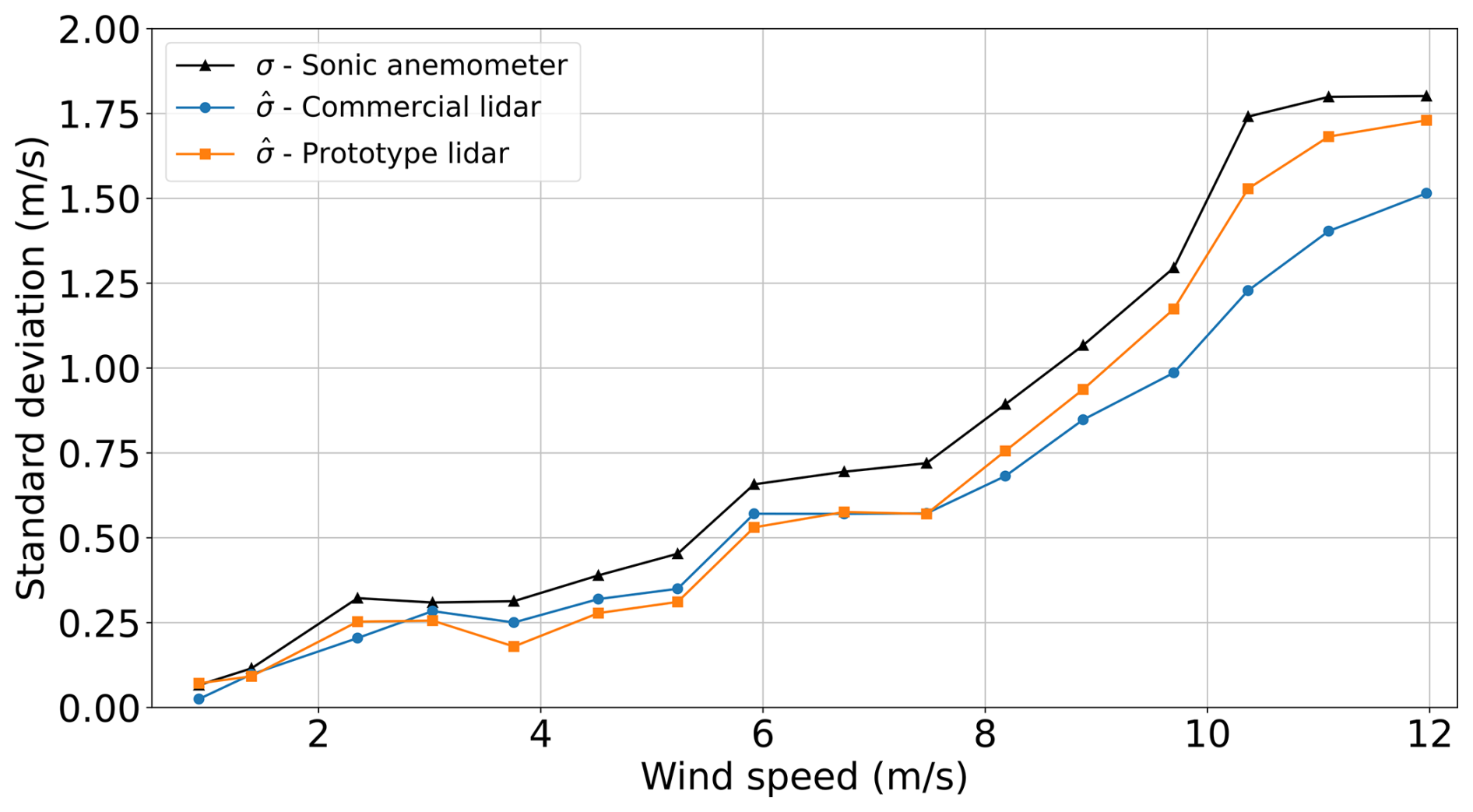
Figure 11 Along-wind standard deviation, $\widehat{\mathit{\sigma }}$, derived from measurements of the commercial lidar (blue curve) and prototype lidar (orange curve) compared to the standard deviation, σ, obtained from reference sonic anemometer measurements (black curve) as a function of wind speed.

4 Discussion

The increased sampling rate resulted in a relatively slight 0.5 % reduction in data availability compared to the commercial configuration over the 47 d dataset. While this difference is minimal, longer measurement campaigns, typically lasting over a year for wind site characterization, may accumulate more instances of data loss due to environmental factors, hardware limitations, or maintenance events, potentially making the impact of reduced availability more noticeable over time. Following the measurement campaign presented in this paper, the prototype configuration was installed in December 2022 on Planier Island in the Mediterranean Sea, where it remains operational. The wind characteristics derived from the full year of 2023 are presented in Thiébaut et al. (2024), including a detailed analysis of data availability. Encouragingly, up to 160 m a.s.l. (meters above sea level), annual data availability exceeded the 90 % threshold considered best practice. Beyond this height, availability gradually declined, reaching below 70 % at 220 m. While this highlights an area for further optimization, the prototype lidar has already demonstrated strong performance at critical measurement heights.

Moreover, the prototype configuration performed comparably to the commercial setup in terms of mean wind characteristics. While the commercial configuration met the best-practice threshold for all key performance indicators (KPIs), the prototype also achieved this standard, with the exception of mean wind speed differences, where it met the minimum-acceptance level within the best-practice range. This result is promising, as it confirms that the prototype lidar meets industry standards, while offering opportunities for further refinement.

Reducing the accumulation time increases the sampling rate, which helps limit the temporal averaging of the wind signal and preserves more of the high-frequency variance within the instrument's resolvable range. However, this also requires a careful evaluation of instrumental noise and its associated variance to ensure that observed changes in variance can be confidently attributed to atmospheric turbulence rather than to measurement artifacts. In this study, the noise-induced variance was estimated using two independent methods. For both lidar configurations, the noise levels were consistent with values reported in previous studies, such as the WindCube lidar analysis by Mann et al. (2009), supporting the reliability of our estimates. As expected, the higher sampling rate of the prototype lidar led to increased instrumental noise due to the reduced number of transmitted pulses (Pearson et al., 2009). The noise variance constituted approximately 5 % of the total variance for the commercial configuration and over 7 % for the prototype. While non-negligible, this contribution was accounted for in all variance-based metrics.

However, the impact of increased sampling must be interpreted with care. If the sampling frequency is too low relative to the turbulent fluctuations present in the flow, aliasing occurs: unresolved high-frequency energy is folded into lower-frequency bands, distorting the spectral distribution. While the reduced accumulation time increases the sampling frequency and helps mitigate aliasing effects, it does not fully recover the true spectral shape, given the finite temporal resolution. Therefore, the observed increase in variance with the prototype lidar should primarily be attributed to reduced temporal and spatial filtering rather than to a direct gain in turbulent energy capture. This distinction is critical.

Increasing the sampling rate does not linearly capture more variance from smaller eddies. Instead, the accumulation time acts as a low-pass filter on the LOS velocity signal, attenuating contributions from high-frequency turbulent fluctuations. Systems with longer accumulation times, such as the 0.8 s used in the commercial lidar, are more affected by this filtering, especially at higher wind speeds where the effective probe length, L_eff, becomes longer due to advection. The effective probe length refers to the spatial distance over which the LOS wind velocity is effectively averaged, accounting for both the fixed probe length and the distance traveled by air during the accumulation period. It can be estimated as

$$\begin{array}{}\text{(11)}& L_{\mathrm{eff}}=L_{\mathrm{probe}}+U\mathrm{\Delta }t.\end{array}$$

A longer effective probe length increases spatial averaging and attenuates variability in the measurements. In contrast, the prototype lidar, with a shorter 0.2 s accumulation time, experiences less temporal averaging and thus preserves a greater portion of the wind variance from smaller-scale motions. This contributes to the higher along-wind variances observed in the prototype configuration compared to in the commercial system. Despite this, the observed increase in variance remains significantly below the theoretical benefit expected from increasing the LOS sampling rate, as determined through sonic anemometer measurements. The measurement volume of a sonic anemometer is effectively point-like in comparison to the much longer probe length of wind lidar profilers. The anemometer is essentially free of the probe time-averaging effect, which enables it to capture the wind signature of very small eddies.

5 Conclusions

The prototype configuration of the WindCube v2.1 lidar profiler demonstrated comparable performance to the commercial system in terms of mean wind characteristics and data availability, meeting industry standards. Moreover, this study demonstrates that increasing the sampling rate of LOS wind velocity measurements by reducing the accumulation time in pulsed wind lidar systems effectively mitigates temporal and spatial averaging effects inside the probe volume, thereby improving turbulence measurements. The prototype configuration, with a 4-fold increase in the sampling rate compared to the commercial system, preserved additional variance by reducing both spatial and temporal averaging rather than by directly resolving smaller eddies, particularly at higher wind speeds, where advection lengthens the effective probe length. Despite these gains, the increased sampling rate introduced trade-offs, including higher instrumental noise and a slight reduction in data availability. The noise was systematically corrected, and its impact was found to be manageable.

The findings underscore the importance of carefully balancing temporal resolution, noise, and probe length when configuring lidar systems for turbulence retrieval. While commercial lidars can be programmed by the manufacturer to match the prototype's sampling rate, it is advisable to validate the lidar's performance through certification after such adjustments. Looking forward, optimizing both accumulation time and probe length in tandem may enhance the ability of wind lidar systems to capture turbulence more accurately. However, such changes must be approached cautiously, as reducing these parameters can also compromise data availability, especially under challenging atmospheric conditions. Balancing resolution and reliability will be key to supporting broader applications in wind energy assessments and atmospheric boundary layer research.