Data-driven probabilistic surrogate model for floating wind turbine lifetime damage equivalent load prediction

Floating offshore wind turbines (FOWTs) experience complex hydrodynamic and aerodynamic loading influenced by substructure types and stochastic environmental conditions. Accurately estimating the lifetime fatigue loads requires the analysis of thousands of operational scenarios, leading to high computational costs. Moreover, choosing the right input features driving fatigue in floating wind systems and appropriately binning them still remains an open question. We present a fast probabilistic surrogate that maps the site conditions to the loads on the wind turbine. The probabilistic aspect allows the propagation and quantification of statistical uncertainties from the stochastic input quantities to the resulting loads. A fast surrogate eliminates the need to fit a distribution to the site conditions or bin the input data. Rather, all available metocean data can be directly used as input, which automatically accounts for the joint distribution in the calculations. The surrogate model in this study uses the mixture density network (MDN) to predict the conditional distribution of the 10 min damage equivalent loads (DELs) for a 6 MW spar-type floating wind turbine. The MDN achieves high accuracy (R²>0.99) in capturing DEL means while efficiently propagating the statistical uncertainties. Furthermore, the surrogate enables quick estimation of 25-year lifetime fatigue damage across a range of potential floating wind farm sites, demonstrating its capability to facilitate rapid decision-making during preliminary site analysis.

1 Introduction

1.1 Background

Floating offshore wind turbine (FOWT) technology has witnessed a surge in research interest in recent years following the rapidly increasing demand for renewable power production. The structural response of an FOWT is a crucial indicator of its performance, safety, and reliability. During its operational lifetime, an FOWT accumulates fatigue damage as it undergoes time-variable loading in response to the complex and stochastic offshore environment. The nature, magnitude, and extent of fatigue are unique to the type of floating foundation, mooring line configuration, wind turbine material, control algorithms, and site conditions.

To ensure a safe and reliable operational life, the FOWT undergoes a certification process involving a rigorous analysis of various design load cases (DLCs) defined by the International Electrotechnical Commission (IEC, 2024a). The first step involves simulating the DLCs on a type-certified rotor-nacelle assembly with a reference tower and floating foundation. More detailed information about the site is included while defining the DLCs as the project progresses. Subsequently, a site-specific tower, foundation, and mooring line configuration are defined, and a site-specific certification study is performed. The calculations are typically made using time-domain multi-physics engineering tools, such as OpenFAST (Jonkman, 2013), HAWC2 (Larsen and Hansen, 2007), and BHawC (Couturier and Skjoldan, 2018; Skjoldan, 2011), throughout this process.

Fatigue is a multi-scale phenomenon that depends on the material composition, composite structure, geometry, and inflow dynamics. The estimation of the fatigue damage for FOWTs, in particular, is computationally intense. The lifetime fatigue load assessment entails calculating the 10 min damage equivalent loads (DELs) on multivariate bins of typical variables characterizing the site and scaling them to the observed probability of occurrence. Not all site variables can be practically included in fatigue load analysis, as the required number of simulations increases exponentially with each additional variable. The choice of the variables in the offshore environment that have the most impact on FOWT fatigue is currently an active area of research (Papi and Bianchini, 2024). The total computational cost of the simulations also constrains the lower limit of the bin size. While industry-standard engineering tools are necessary for certification, the preliminary site analysis can benefit from data-driven surrogate models to provide quick load estimates. Data-driven surrogates can infer complex relationships from data observations alone and do not require prior knowledge of the underlying physics. Fatigue, which is difficult to model using lower-fidelity physics-based approaches, can benefit from such data-driven methods. Using surrogates that can accurately predict DELs can potentially eliminate the need to bin the site data, fit a multivariate joint distribution to it, or limit the total number of parameters. Once trained, surrogate models can directly use all the available site information to estimate the site-specific DELs quickly. In addition, probabilistic surrogates can also propagate the statistical uncertainty from the stochastic input variables to the loads.

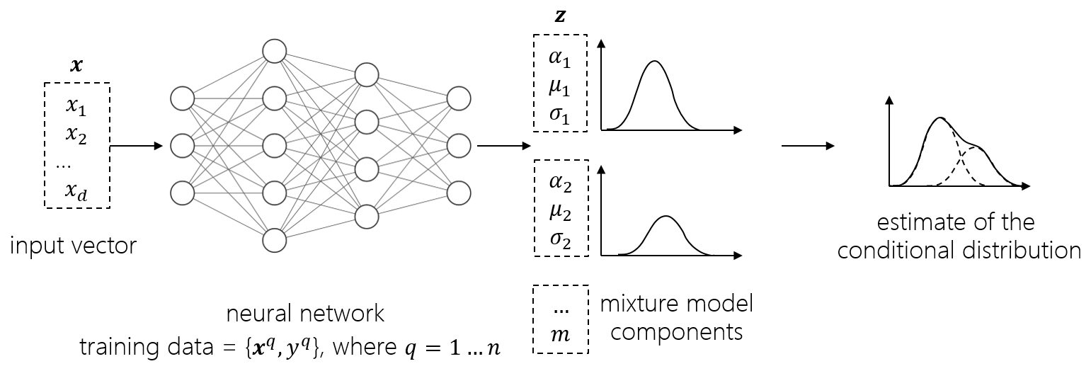
Data-driven surrogates for wind turbine or wind farm level loads are often designed with deterministic models. Given a training dataset with d-dimensional input parameters x∈ℝ^d, the deterministic surrogate maps them to the corresponding output observations y∈ℝ. However, the assumption of a deterministic relationship between inputs and outputs does not hold in our case. For instance, keeping every other input constant, a single value of 10 min mean wind speed can correspond to an infinite number of turbulent inflow patterns, resulting in an infinite number of DEL values with a certain probability distribution conditioned on that wind speed. Probabilistic surrogates model the statistical uncertainty in the input variables by representing them as a random variable X with a joint probability density function (PDF). The corresponding output is, therefore, also a random variable denoted as Y.

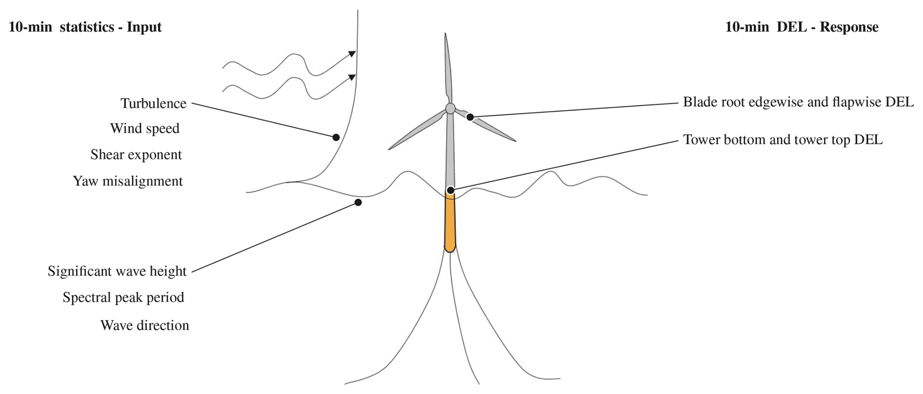
This study is focused on using a probabilistic data-driven surrogate to map 10 min statistics of the environmental conditions to the corresponding conditional probability distribution of the DEL on the floating spar buoy with a 6 MW Siemens Gamesa wind turbine. The DEL values are calculated using the Siemens Gamesa in-house tool that couples the aeroelastic code, BHawC (Skjoldan, 2011), with the hydrodynamic solver, OrcaFlex (Arramounet et al., 2019). A schematic of this mapping is shown in Fig. 1. A highly flexible probabilistic machine learning approach for the surrogate, the mixture density network (MDN) (Bishop, 1994), is used in this study. The probabilistic estimates of DELs are used to subsequently calculate the lifetime fatigue loads at various potential floating wind sites.

Figure 1 Schematic of the surrogate modeling objective.

1.2 Previous work on probabilistic data-driven modeling for wind turbine load estimation

The standard Gaussian process regression (GPR) (Rasmussen and Williams, 2006) is one such probabilistic surrogate that is capable of uncertainty quantification. However, in its standard form, it is restricted to normally distributed homoscedastic responses. Nevertheless, due to its flexibility and ease of implementation, it is widely used as a surrogate to estimate the fatigue load response in wind turbines (Teixeira et al., 2017; Avendaño-Valencia et al., 2021; Li and Zhang, 2019, 2020; Gasparis et al., 2020; Dimitrov et al., 2018a; Slot et al., 2020).

Further interest in quantifying the uncertainty of the short-term fatigue loads as a function of the input parameters has initiated research into heteroscedastic surrogates. Heteroscedasticity refers to the heterogeneity in the response variance as a function of the inputs. The variance observed in DEL at the tower bottom, for instance, for very large values of significant wave height, is generally larger than that in calm ocean conditions. It is, therefore, an important consideration when choosing the appropriate surrogate modeling approach for load uncertainty quantification. Murcia et al. (2018) use 100 turbulent inflow realizations at each sample point to obtain the first two moments of the fatigue response. Thereafter, they create two independent surrogates using polynomial chaos expansion (PCE) to model the mean and standard deviation of the fatigue loads on the DTU 10 MW reference wind turbine. Even though they use only 140 training samples for their model, the replications scale the computational cost by 100, eventually leading to a costly training database. Another replication-based approach is taken by Zhu and Sudret (2020) to model the load response using generalized lambda distributions. In this study, 50 inflow wind field realizations are used at each input sample to estimate the four lambda parameters. Four PCE surrogates are then used to model the parameters independently. The main drawback of replication-based methods is the cost of generating the training database, which makes it challenging to apply them to computationally demanding applications such as floating wind turbines. Secondly, the goodness of fit relies heavily on estimating the statistical parameters in the first step.

Heteroscedasticity can also be modeled using statistical methods. Zhu and Sudret (2021) extend the replication-based approach to derive a statistical method combining generalized least-squares with maximum conditional likelihood to estimate the lambda parameters without replications. The main advantage of this method is that it does not assume a Gaussian distribution. However, it cannot handle multimodality.

Abdallah et al. (2019) use parametric hierarchical Kriging to predict blade-root-bending-moment extreme loads that are heteroscedastic on a 2 MW onshore wind turbine. Their approach combines low- and high-fidelity observations, where the low-fidelity model informs the high-fidelity GPR. They show that introducing hierarchy helps make the model selection process more robust than the manual tuning of GPR parameters. Singh et al. (2022) apply chained GPR that uses variational inference within a Bayesian framework to account for heteroscedasticity in the data and make predictions of site-specific load statistics on a more complex case of offshore wind turbines. The model can capture the heteroscedasticity in a small dataset but is not scalable to high-dimensional problems. To address the scalability constraints, the authors extend the study to use mixture density networks on the same dataset to quantify the uncertainty in the load response (Singh et al., 2024a). The application of probabilistic surrogates to floating wind turbines has only been studied to a limited extent in the literature. Li and Zhang (2019) model the uncertainty in the site conditions using a C-vine copula combined with artificial neural networks and GPR. Heteroscedastic probabilistic data-driven modeling has been further explored using Bayesian neural networks (BNNs) for estimating loads on non-instrumented wind turbines using information from fully instrumented counterparts (Hlaing et al., 2024). Preliminary studies on fatigue load prediction using BNNs show promising results in onshore wind turbines (Omole et al., 2021). BNNs are a powerful class of neural network architectures that assign probability distributions to the network weights and biases, effectively allowing the separation of aleatoric and epistemic uncertainties.

In summary, only a few approaches attempt to model the uncertainty in the load response of the turbine and the tower. Of those that do, only some consider complex offshore floating systems. This presents a key research gap as the dynamic behavior of floating platforms introduces additional complexity not present in fixed-bottom systems. Following the promising performance of mixture density networks (MDNs) for fixed-bottom wind turbines (Singh et al., 2024a), in this study, we aim to extend the framework to a more complex application of a spar-buoy-type wind turbine case. In the case of MDN, the target is modeled as a mixture of m∈ℕ Gaussian kernels of varying proportions, capable of generating complex distributions when combined. MDN uses feed-forward networks to learn the parameters of the mixture model.

1.3 Research objectives

The objectives of this work are 3-fold:

• To apply and evaluate a probabilistic machine learning model (MDN) for predicting short-term fatigue loads in floating offshore wind turbines.

  Not only are FOWT loads affected by the nonlinear dynamic behavior of the floating wind turbine, but the underlying simulations are also much more complex, the stochastic hydrodynamic parameters have a bigger impact on the tower, the data is “noisier”, the parameter space is larger, and thereby, the number of simulations is large. This necessitates investigations into robust surrogates. Probabilistic data-driven models are often validated on simpler cases. Complex cases are modeled using deterministic approaches or with the assumption that the response is Gaussian or homoscedastic. Using a mixture model effectively solves many of the gaps in the literature by propagating uncertainty, including heteroscedasticity, and modeling higher-order moments.

• To demonstrate that such a model can provide insights into probabilistic long-term fatigue estimation, especially in high-dimensional spaces where traditional binning approaches become computationally restrictive.

  The lifetime fatigue estimation for FOWTs involves additional complexity, including the joint distribution of metocean conditions and sensitivity to bin sizing. These issues are exacerbated by the exponential growth in simulation cost with each added dimension. A surrogate model enables direct use of historical site condition data, bypassing the need for parametric joint distribution assumptions.

• To investigate the impact of stochastic variability in site conditions on fatigue prediction over long time spans.

  We select four potential floating wind sites with similar water depths and use the surrogate model to estimate probabilistic lifetime fatigue loads. We investigate the effect of accounting for the stochastic variability in the 10 min loads relative to the variation in site conditions. It is demonstrated that, due to the law of large numbers, the influence of random seeds on long-term tower load estimation diminishes significantly over a 25-year period, even with 500 seeds (from the probabilistic surrogate). This indicates that stochastic inflow conditions contribute minimally to uncertainty in long-term fatigue predictions.

By addressing these points, this work contributes a validated, flexible surrogate modeling framework that accounts for the complexities of floating wind systems, advancing the state of probabilistic load modeling in floating offshore wind research.

The rest of the paper is structured as follows. In Sect. 2, we introduce the floating wind turbine model, describe the simulation tools used, and outline the input features, including their ranges and the sampling strategy. Section 3 then presents the theoretical foundation of the mixture density network (MDN), discusses the chosen hyperparameters, and explains the criteria for evaluating model performance. The results, presented in Sect. 4, are divided into three subsections. First, we analyze how the model's performance converges across a range of training samples. Next, we validate the selected MDN model's 10 min conditional distribution estimates under randomly chosen operating conditions, comparing them with those generated by BHawC. Finally, we demonstrate how the probabilistic 10 min estimates can be used to propagate the statistical uncertainty to the lifetime fatigue damage. Concluding remarks are provided in Sect. 5.

2 Setup

2.1 Definition of the floating wind turbine

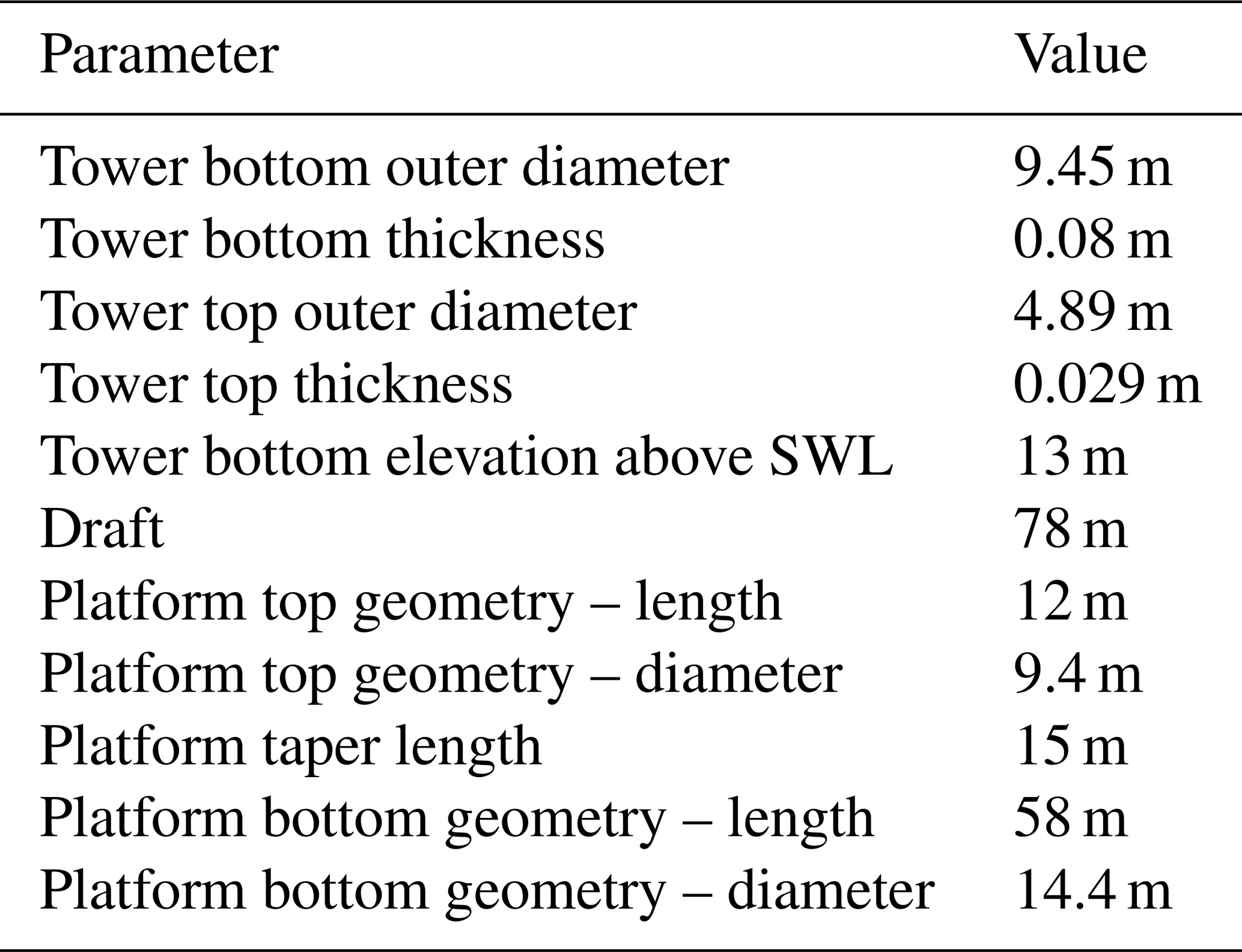
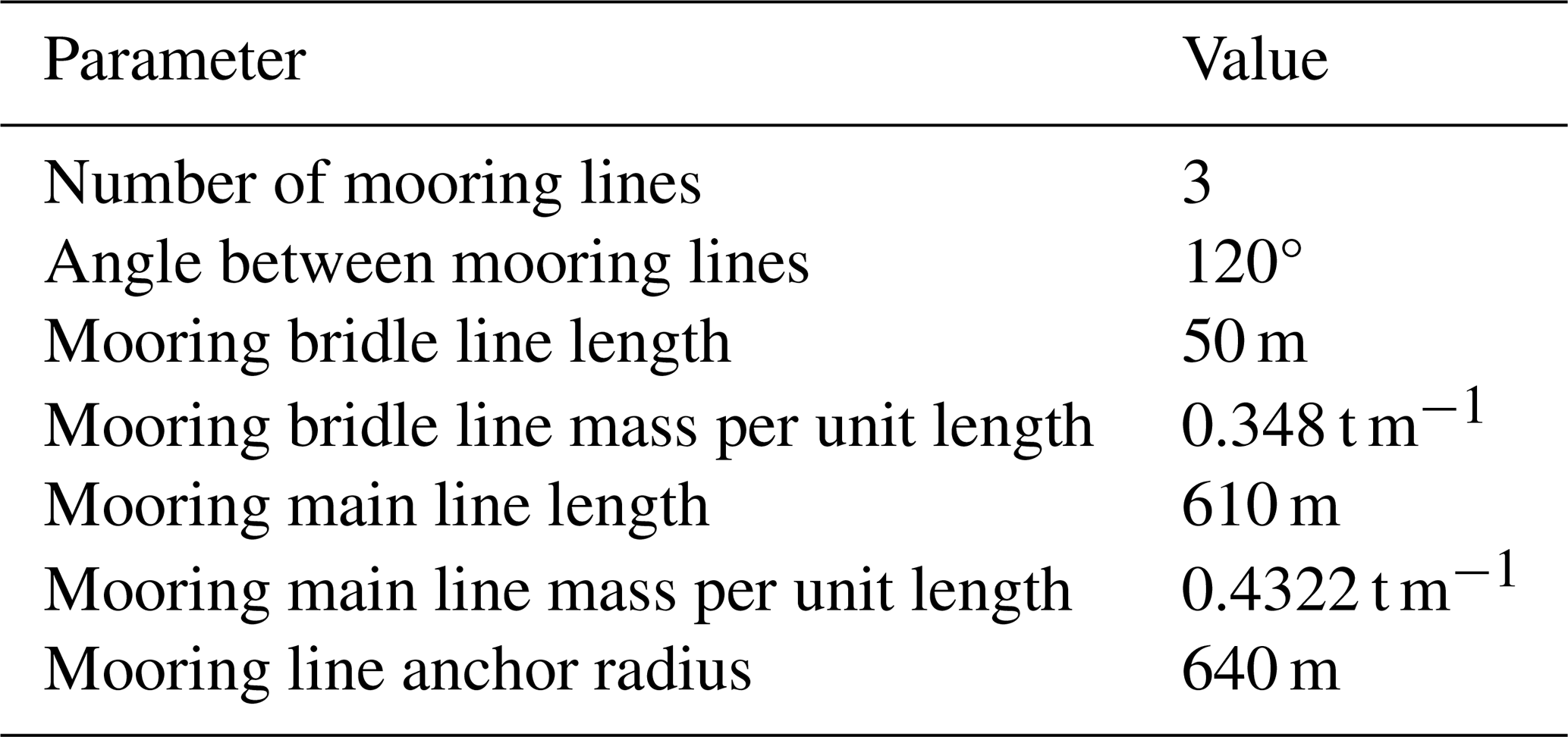
The floating wind turbine in this study is based on a modified geometry of the Hywind Scotland spar buoy foundation (Equinor ASA, 2022). It comprises a 6 MW Siemens Gamesa Renewable Energy direct drive wind turbine assembly, SWT-6.0-154, mounted on a spar buoy. The characteristic wind turbine parameters are listed in Table 1. The simulations use a tower with a larger diameter than the tower designed for the Hywind Scotland site. It is, therefore, stiffer and has a higher natural frequency than its installed counterpart. The geometry details of the tower and the floating platform used in the simulation are provided in Table 2. The floating substructure is attached to the ocean floor using catenary mooring lines, equally spaced at 120° in crowfoot configuration using bridle lines as shown in Fig. 2 (Equinor ASA, 2022). The structural properties of the main mooring lines and the bridle lines are listed in Table 3.

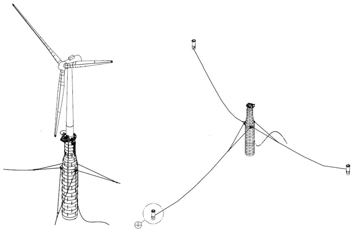
Figure 2 Hywind Scotland spar buoy with crowfoot mooring line configuration (Equinor ASA, 2022).

Table 1 Parameters of 6 MW Siemens Gamesa wind turbine.

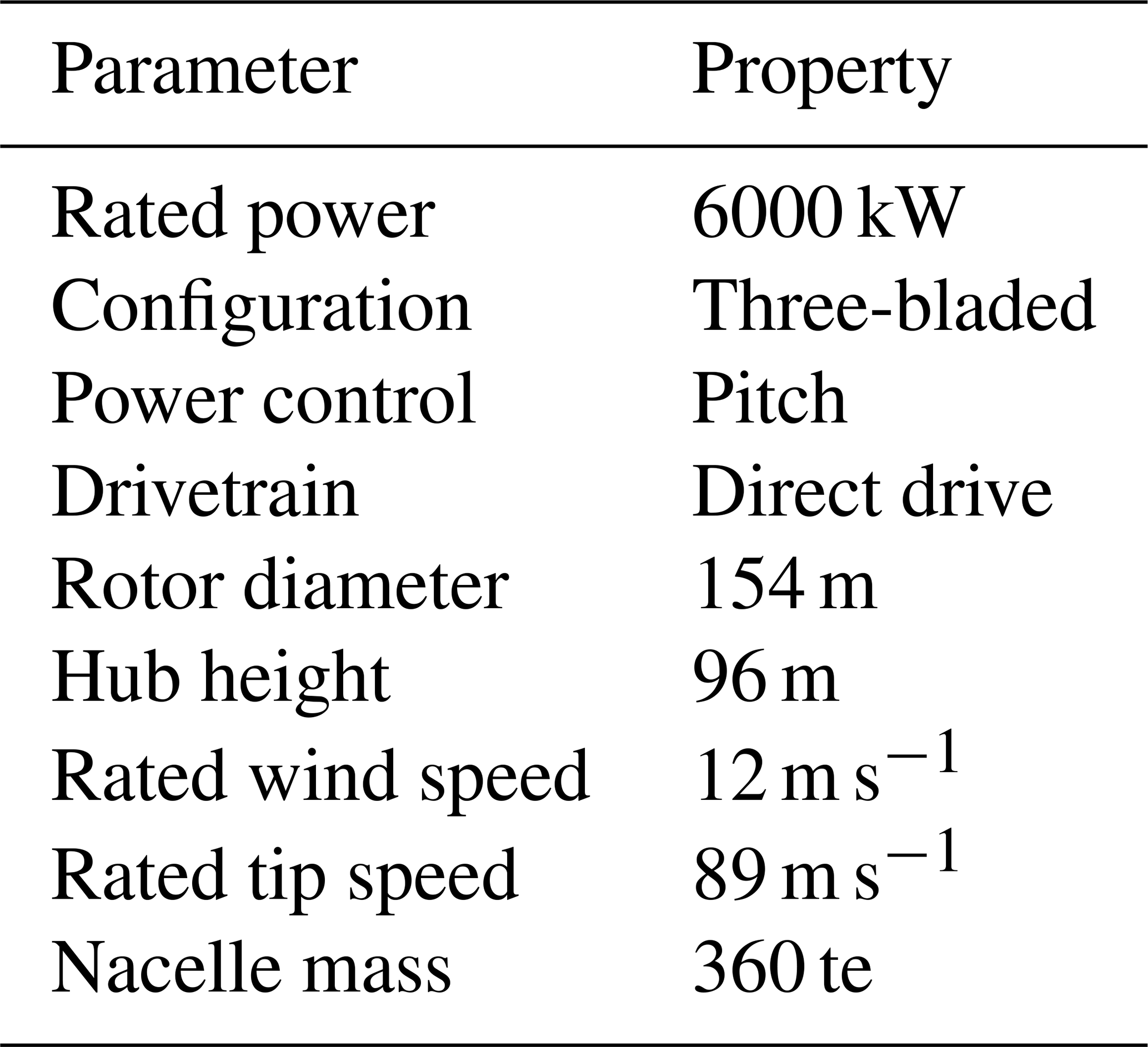
Table 2 Wind turbine tower and foundation properties (Bussemakers, 2020; Equinor ASA, 2022; Equinor, 2024).

Table 3 Catenary mooring line properties.

2.2 Numerical model

The damage equivalent loads are obtained through time-domain hydro-servo-aeroelastic simulations performed using BHawC–OrcaFlex-coupled implementation. BHawC has been used for several years at Siemens Gamesa for wind turbine load calculations and is continuously validated against turbine prototypes and the entire operational fleet. Similar analysis may be performed with OpenFAST (NREL, 2022; Jonkman, 2013) coupled with OrcaFlex (Masciola et al., 2011) via FASTLink for reproducibility. Arramounet et al. (2019) present the mathematical background for the software coupling. In short, the tower, the rotor nacelle assembly, and the blade elements are dynamically modeled in BHawC. The BHawCLink module acts as a communication channel with the dynamic link library, connecting it to the OrcaFlex API. OrcaFlex simulates the hydrodynamic response of the floater element. Time integration is performed individually on both elements while accounting for the response of the other structure per iteration (Arramounet et al., 2019).

The inflow turbulence is modeled using a spatially varying frozen wind field based on the Mann model (Mann, 1998). The tangential and axial induced velocities are calculated on several aerodynamic nodes on the blades using the blade element momentum theory coupled with Prandtl's tip loss correction and thrust correction at high induction values. Skewed and unsteady inflow is modeled using the method introduced by Björck (2000).

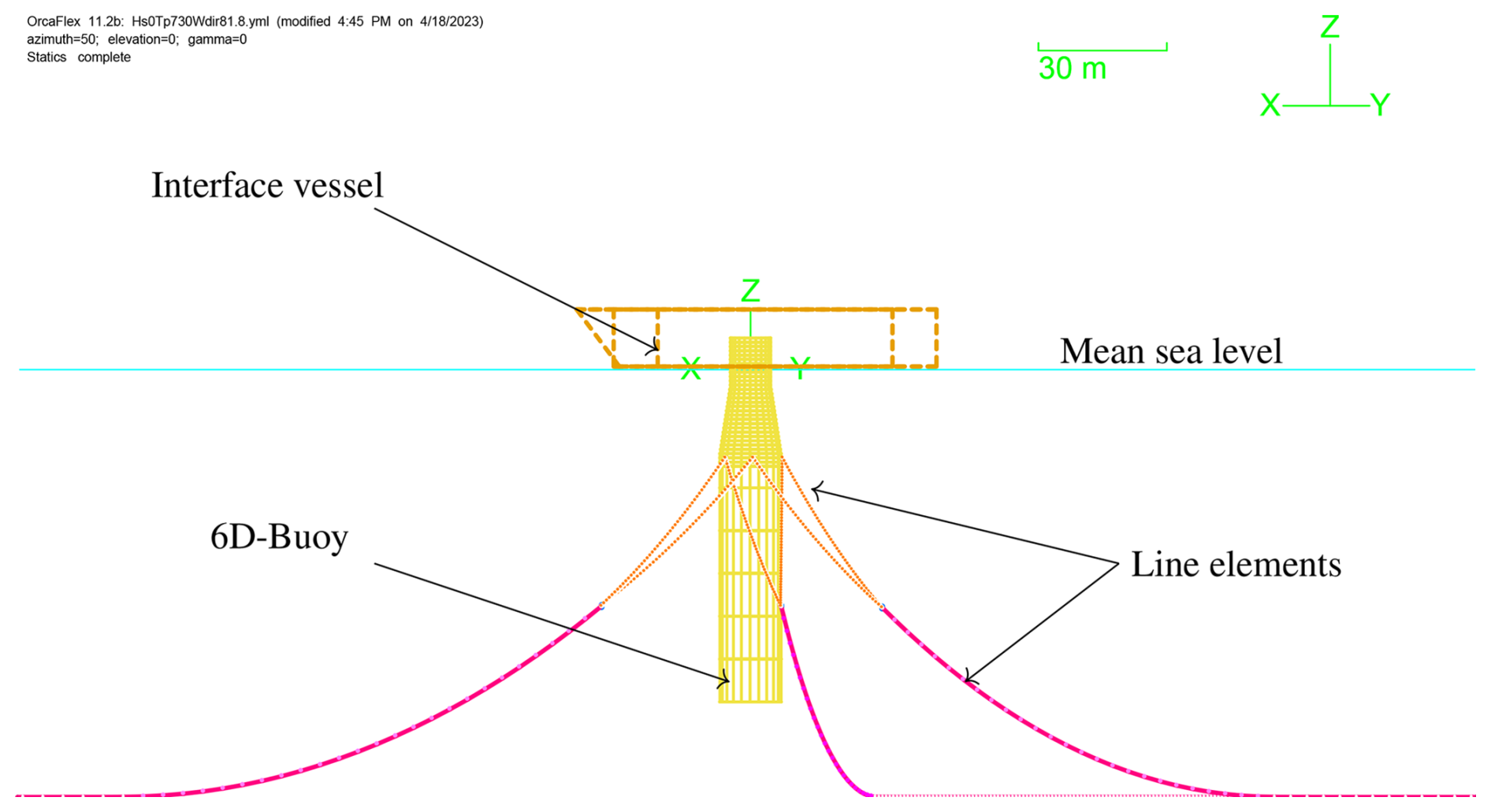
The structural elements are modeled using the co-rotational formulation, providing geometric nonlinearity (Rubak and Petersen, 2005). The tower, shaft, and blade substructures are modeled using beam elements (Couturier and Skjoldan, 2018). The Torsethaugen two-peak wave spectrum generates swell and local wind-driven waves (Torsethaugen and Haver, 2004). The various elements of the OrcaFlex model are shown in Fig. 3. A 6-DOF rigid buoy in OrcaFlex represents the floating substructure. The mooring lines are modeled in OrcaFlex. Each line is divided into several massless spring segments, joined by elements with lumped properties such as mass, damping, added mass, buoyancy, and material properties.

Figure 3 Schematic of the OrcaFlex simulation elements.

The simulations are initialized in BHawC with a quasi-static approach where the environmental loads (wind) and inertial loads (gravity and buoyancy) are ramped up in small steps. For every load step, OrcaFlex determines the mooring line static equilibrium based on the floater position determined by BHawC. BHawC calculates the global equilibrium position based on the stiffness matrices and interface loads provided by OrcaFlex. Once the global equilibrium is calculated, the next load step is applied. The dynamic part of the simulations consists of an initialization phase of 300 s to eliminate any initial transients as the wave dynamics, turbulence, and substructure motion build up as the artificial structural damping is slowly ramped down. The final post-processing is performed on 600 s dynamic simulations that follow the initialization phase. The simulations for training the surrogate may be performed for a longer duration if necessary, mainly to estimate mooring line fatigue correctly due to its long natural period. The effect on the tower and blade fatigue is shown not to change significantly with larger simulation windows but rather with the fatigue calculation algorithm used to account for the unclosed cycles (Stewart et al., 2013).

2.3 Definition of relevant site features and responses

Having a large feature space can lead to a very expensive surrogate training process, as the number of training samples required grows rapidly with the number of input variables due to the curse of dimensionality. It is, therefore, important to identify which variables have the most significant impact on fatigue to reduce the input space effectively.

Several studies in the past have focused on addressing the sensitivity of wind turbine loads to environmental conditions (Robertson et al., 2018, 2019; Teixeira et al., 2019; Shaler et al., 2023; Singh et al., 2024c). The combined effect of environmental and structural parameters has been analyzed on fixed-bottom (Hübler et al., 2017; Velarde et al., 2019; Dimitrov et al., 2018b) and floating wind turbines (Wang et al., 2023; Wiley et al., 2023; Lin et al., 2021; Reddy et al., 2024; Singh et al., 2024c).

Wiley et al. (2023) demonstrate that, for the OC4-DeepCwind semi-submersible platform, the standard deviation of wind speed in the inflow is the most influential parameter affecting the fatigue and ultimate loads on the tower and blades. Secondary drivers of fatigue on the tower bottom moment include both turbulence coherence parameters and wave characteristics, such as significant wave height and peak spectral period. For blade pitching fatigue, secondary factors include the yaw misalignment angle and geometric features like the blade twist angle, whereas the wind–wave misalignment and the current speed and direction seem to have a secondary effect on the blade-root-bending-moment fatigue. Reddy et al. (2024) perform elementary effects analysis to determine the most significant parameters affecting tower bottom fatigue on the OC3-Hywind Spar platform and the OC4-DeepCwind semi-submersible design. In both cases, the significant wave height is found to be the primary driver. Current-related parameters are shown to have a strong effect, mainly on the mooring line fatigue. Singh et al. (2024c) use measurement data from the TetraSpar demonstrator to find that the tower and blade fatigue are most highly correlated with the wind speed mean and standard deviation and with significant wave height values.

As observed, although current has a big impact on the mooring line loads, its effect is found to not be as significant on the tower and blades in the literature. Therefore, it is not included as a variable feature in the training of the surrogate. A variation in the water depth was also not considered because the mooring line system must be redesigned for any new value of water depth. A framework for automating this process is non-trivial. Furthermore, for slack mooring lines, Lin et al. (2021) show a negligible impact on the tower fatigue with an increase in water depth.

Table 4 The list of input features provided to the surrogate model and their corresponding notation.

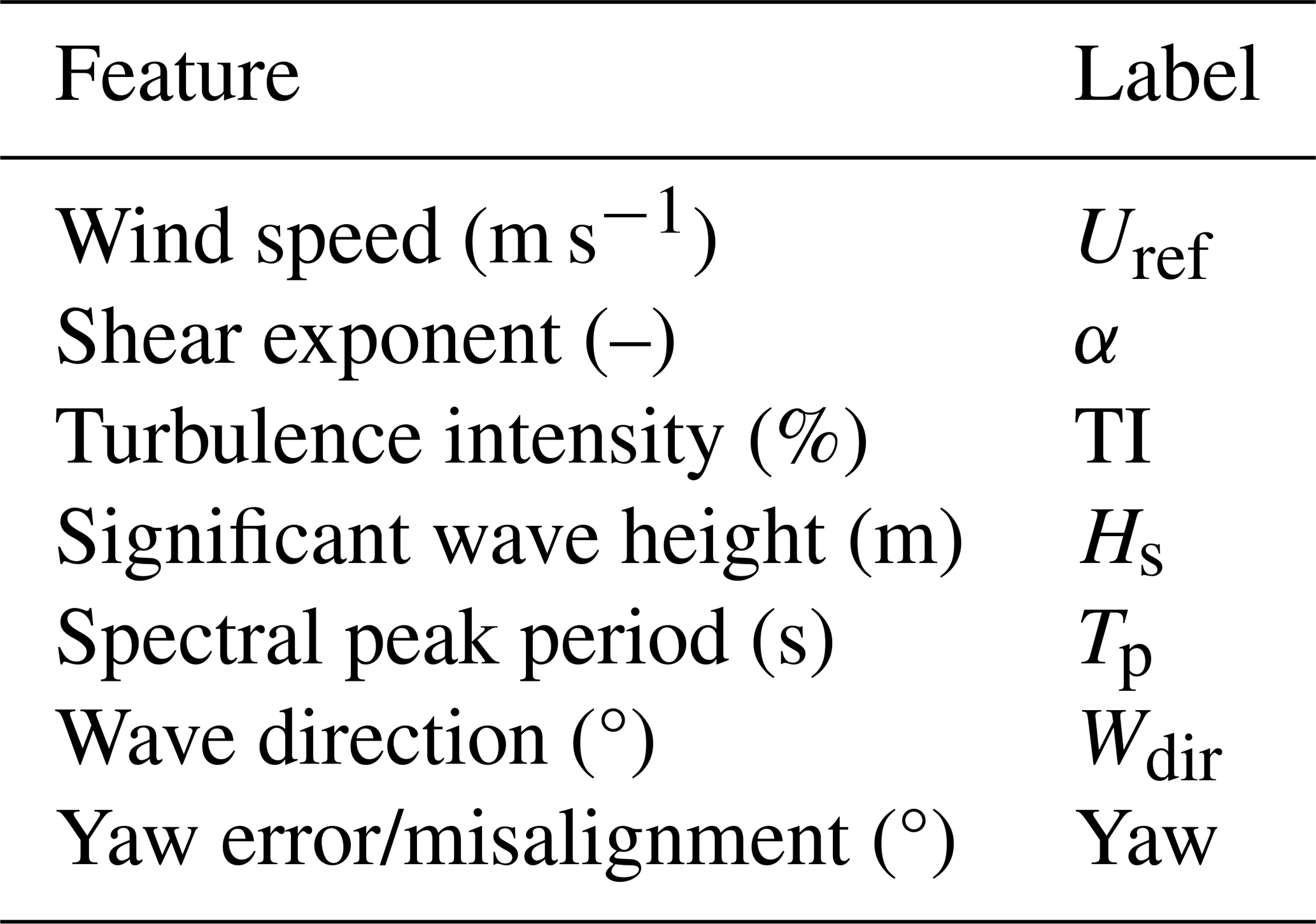
Table 5 The list of output channels that the surrogate models are trained to predict.

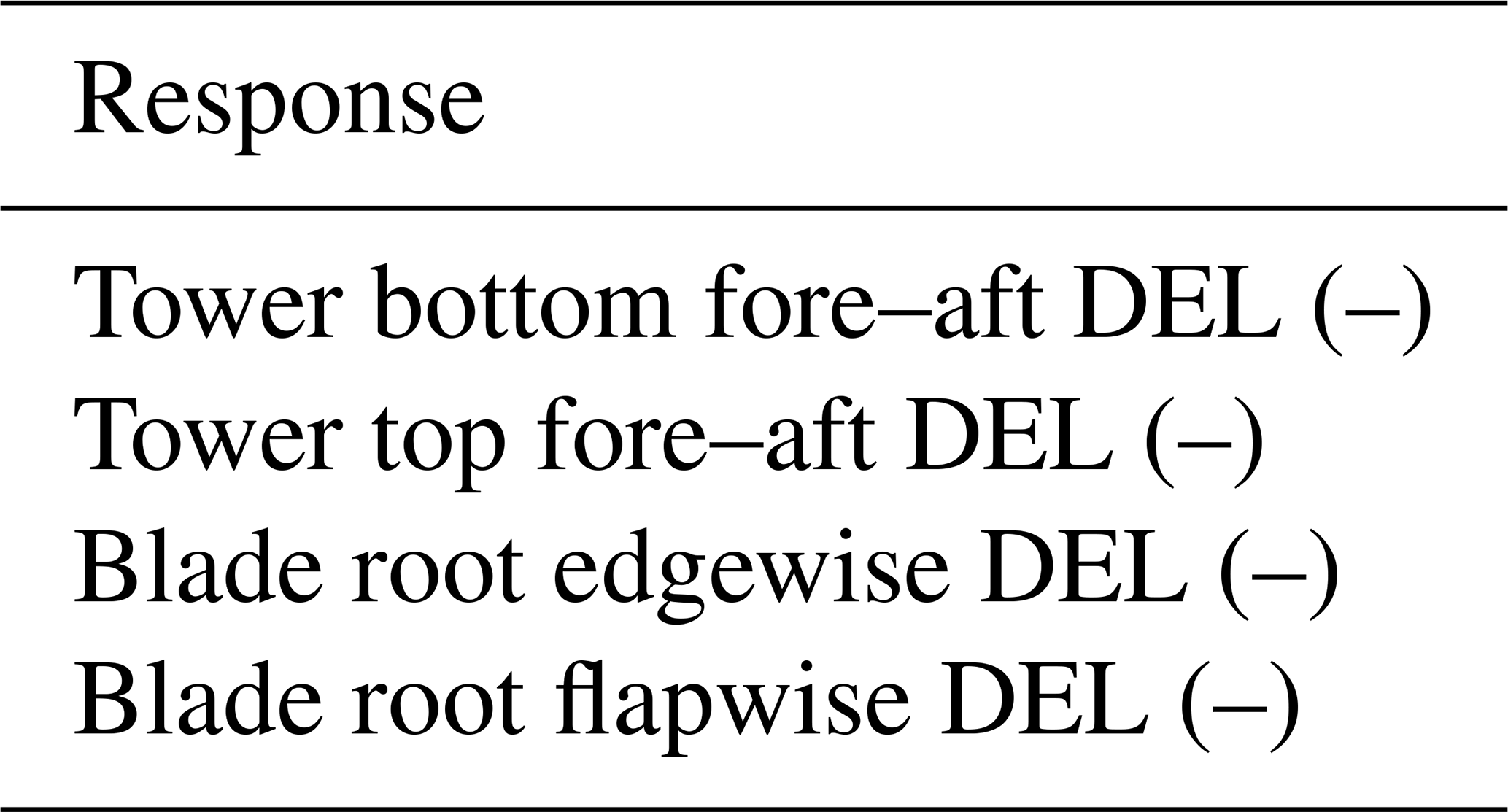
The targets the surrogates are trained on are listed in Table 5. Each target is trained with a separate surrogate model. This study only calculates the short-term DELs in the local coordinate system of the component. DELs result from the conversion of the irregular load time series to a constant amplitude and frequency signal that produces an equivalent fatigue damage. The Rainflow counting (Matsuishi and Endo, 1968) algorithm is used to obtain the load ranges S_i and the number of load cycles n_i needed to calculate the DEL as

$$\begin{array}{}\text{(1)}& \mathrm{DEL}:={\left({\displaystyle \frac{\sum n_i{S}_i^m}{n_{\mathrm{ref}}}}\right)}^{\mathrm{1}/m},\end{array}$$

where n_ref is 600 for 1 Hz DELs over 10 min. m is the Wöhler coefficient with values of 3.5 for the tower, 10 for blade flapwise moments, and 8 for blade edgewise moments. Finally, Z-score normalization is used to scale the DEL to its dimensionless form.

2.4 Feature bounds

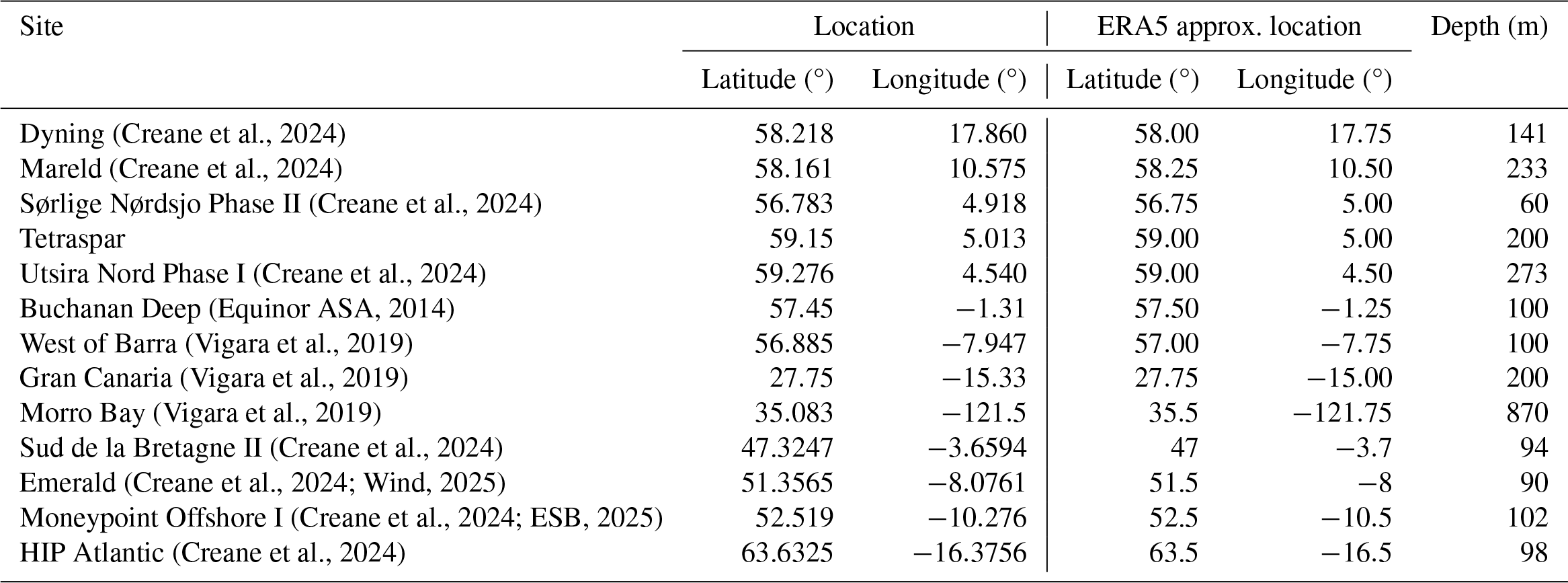
The feature bounds are defined based on the observations of data on sites where floating wind farms could potentially exist (Creane et al., 2024) and where data were readily available. Table A1 in Appendix A lists the selected sites with their location and water depth values. The ERA5 reanalysis data, produced by the European Center for Medium-Range Weather Forecasts (ECMWF) on behalf of the European Union's Copernicus Climate Change Service (C3S), is used for the analysis in this section.

2.4.1 Average wind speed at hub height

The wind speed at hub height (U_ref) varies between 3 and 28 m s⁻¹, which is the operational range of the wind turbine investigated in this study.

2.4.2 Shear exponent

The shear exponent α is defined according to the wind profile power law as

$$\begin{array}{}\text{(2)}& {\displaystyle \frac{U}{U_{\mathrm{ref}}}}={\left({\displaystyle \frac{z}{z_{\mathrm{ref}}}}\right)}^{\mathit{\alpha }},\end{array}$$

where U is the wind speed at height z and U_ref is the known wind speed at height z_ref. We used the ERA5 reanalysis data to obtain wind speed values at 10 and 100 m for the sites listed in Table A1. Assuming the wind profile follows the power law, the shear exponent is calculated using Eq. (2). The distribution of the shear exponent is shown in Fig. 4a, with values primarily ranging between 0 and 0.2. It is also plotted against wind speed in Fig. 4b. In our database, the shear exponent is uniformly distributed in the region corresponding to the dashed box in Fig. 4b.

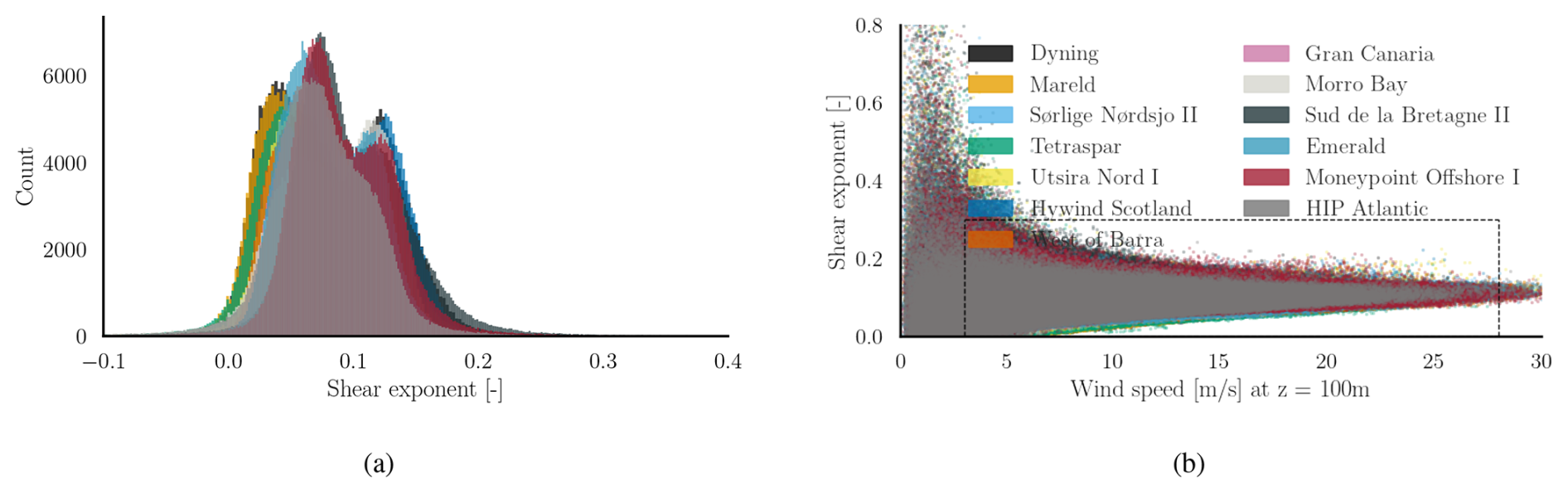
Figure 4 (a) Histograms of the shear exponent α for selected sites for ERA5 reanalysis data from 1990 to 2019. (b) Shear exponent shown as a function of wind speed, marked by a box denoting the selected sampling domain.

2.4.3 Turbulence intensity

The lower range of turbulence intensity is 0.1 %, and the upper limit is designed to be 20 % greater than the prescribed IEC Class C standard (IEC, 2010) for the Normal Turbulence Model (NTM). The function for class C turbulence intensity (in percent) is given by

$$\begin{array}{}\text{(3)}& \mathrm{TI}=\mathrm{100}\times {\displaystyle \frac{I_{\mathrm{ref}}(\mathrm{0.75}{V}_{\mathrm{hub}}+\mathrm{5.6})}{V_{\mathrm{hub}}}},\end{array}$$

where I_ref=0.12 is the expected value of turbulence intensity at 15 m s⁻¹. The upper limit of turbulence intensity for sampling is, therefore, 1.2×TI. Figure 5 shows the chosen range, with the IEC class C turbulence and the measured turbulence at the FINO 3 metmast, which is referenced in the Buchanan deep metocean report (Equinor ASA, 2022).

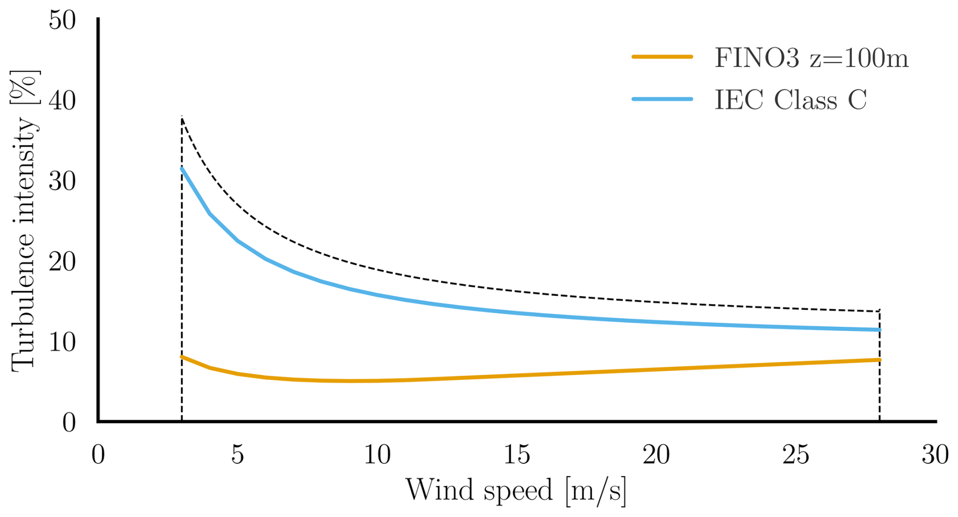
Figure 5 Chosen turbulence intensity range in dashed lines, along with the IEC class C turbulence profile for NTM and measured turbulence at FINO 3 (German Bight) from the metocean analysis report on the Hywind Scotland project (Equinor ASA, 2022).

2.4.4 Significant wave height

Waves in deep water primarily originate from two sources: wind-induced waves and swell waves. It is useful to consider the correlation between wind speed and significant wave height while training the surrogate to avoid including non-physical wind–wave combinations. Figure 6a illustrates a scatter plot of significant wave height (H_s) versus wind speed, based on ERA5 reanalysis data for the selected sites. The sampling domain is also a function of wind speed, highlighted with the dashed lines.

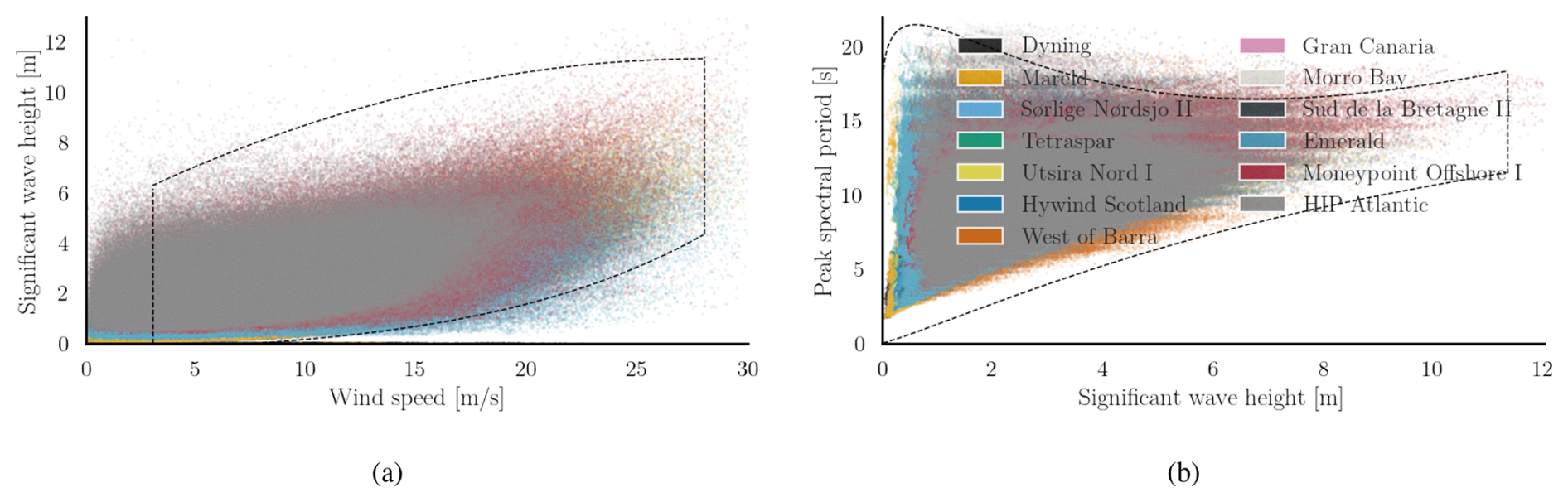
Figure 6 Scatter plots of (a) the significant wave height (H_s) vs. the wind speed (U_ref) at 100 m and (b) peak spectral period (T_p) vs. significant wave height (H_s) for the selected sites (Table A1) based on the ERA5 reanalysis data from 1990 to 2019.

The upper and lower ranges of sampling for the significant wave height are defined empirically based on these observations. In this case, the functions are rather conservative and subject to modification based on the kinds of sites the user would want to use the surrogate model on. The equations for the upper and lower limits for H_s are listed in Appendix B1.

2.4.5 Peak spectral period

The empirical functions are defined for the spectral period range based on the significant wave height. Figure 6b illustrates the sampling domain with dashed lines, overlaid on observational data from the ERA5 reanalysis. This plot also includes H_s−T_p values corresponding to wind speeds below the cut-in speed and above the cut-out speed. The functions defining this range are detailed in Appendix B2. As with the significant wave height, these bounding functions can be adjusted based on the region of primary interest to the user.

2.4.6 Wave direction

The wind turbine is always assumed to face the inflowing wind. Therefore, only the wave direction is varied to introduce wind–wave misalignment. Wave direction is considered to be an independent variable and is sampled uniformly between 0 and 360°. For asymmetric floating foundations, however, wind directions would also need to be considered as an independent parameter.

2.4.7 Initial yaw misalignment

The effect of the initial yaw misalignment is chosen to be evaluated at −5.6, 0, and 5.6° while fatigue calculations are performed. Therefore, we selected the sampling bounds between $\mathrm{1.1}\times -\mathrm{5.6}$° and 1.1×5.6°.

2.5 Training and testing database generation

2.5.1 Training database

Sobol' sampling (Sobol, 1967) is used to jointly sample uniformly in seven dimensions to generate the training dataset. The samples lying outside the aforementioned feature bounds are discarded, resulting in a total of 9041 training samples. Alternatively, a multivariate distribution fitting the available data can be used to define the sampling space bounds. Each sample corresponds to a unique wave seed in OrcaFlex and a single inflow turbulence seed in BHawC. This approach is designed to emulate the inherent stochasticity of real-world inflow variables. Note that the statistical variation in the flow field is constrained by the BHawC implementation to only 45 turbulence seeds. Consequently, these seeds had to be reused, and the inflow turbulence box could not be uniquely defined for every case.

2.5.2 Testing database

The values of the shear exponent, turbulence intensity, and yaw misalignment are not randomly assigned to the test cases. Instead, they take the values used commonly while performing fatigue design load case evaluations. The shear exponent was fixed at 0.08, with yaw misalignment values of −5.6, 0, and 5.6° and turbulence intensity corresponding to IEC Class C values. H_s, T_p, TI, and U_ref were jointly sampled in a random manner, without being tied to any specific location but constrained within the defined feature bounds. For future studies, jointly sampling the test points across all variables is recommended for a fairer evaluation of the surrogate's performance.

In total, n_test=47 test samples were used in this study. Each test sample simulation was repeated with n_seeds=44 random seeds for turbulence and waves to capture the statistical variation in the DEL values from the variation in the wind and wave fields. The seed repetition establishes a reference conditional distribution for each sample, which is used to compare against the probabilistic predictions of the surrogate model in Sect. 4.2. The samples used for training and testing the surrogate models are shown in Fig. 7.

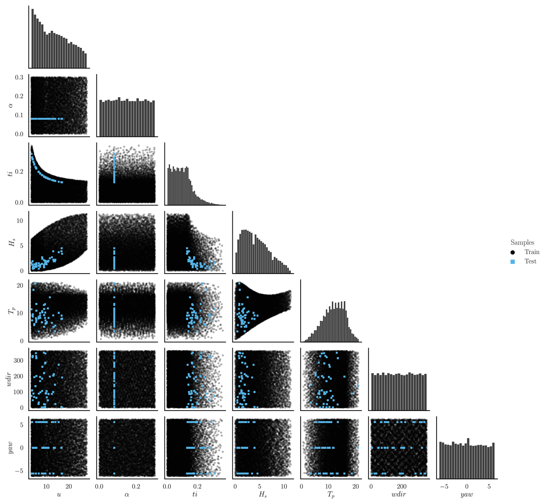
Figure 7 Paired scatter plots and marginal distributions of the training and testing datasets.

3 Methodology

This section briefly describes the theoretical basis of the mixture density network models investigated in this study, along with the accuracy metrics considered to evaluate the surrogate's goodness of fit. The database $\mathit{\{}{\mathit{x}}^q,y^q{\mathit{\}}}_{q=\mathrm{1}\mathrm{\dots }n}$ consists of n pairs of inputs x∈ℝ^d and the corresponding output y∈ℝ. The surrogate is calibrated separately for each target.

3.1 Mixture density networks

A mixture density network is a probabilistic regression method that combines Gaussian mixture models with artificial neural networks (Bishop, 1994). The conditional distribution of the target is represented as a linear combination of m∈ℕ Gaussian kernel functions,

$$\begin{array}{}\text{(4)}& p(y\mid \mathit{x})=\sum _{i=\mathrm{1}}^m{\mathit{\alpha }}_i\left(\mathit{x}\right)\mathcal{N}(y\mid {\mathit{\mu }}_i(\mathit{x}),{\mathit{\sigma }}_i^{\mathrm{2}}(\mathit{x}\left)\right),\end{array}$$

where α_i(x) is the weights or mixing coefficients assigned to the ith mixture component. A schematic of MDN is shown in Fig. 8. $\mathcal{N}(y\mid {\mathit{\mu }}_i(\mathit{x}),{\mathit{\sigma }}_i^{\mathrm{2}}(\mathit{x}\left)\right)$ is a Gaussian kernel representing the conditional density of the ih component of the target distribution, with parameters μ_i(x) and σ_i(x). Instead of mapping the inflow features x to the load statistics y directly, the neural network is trained to predict the parameter vector, z∈ℝ, consisting of α_i(x),μ_i(x), and σ_i(x) for $\mathrm{1}<i<m$ (Singh et al., 2024b).

Figure 8 Schematic representation of mixture density networks.

The mixing coefficients α_i(x) must sum up to exactly 1. A softmax function is used to handle this constraint. Positive values of the standard deviation are ensured by their representation as exponential functions of the corresponding network outputs, $z_i^{\mathit{\sigma }}$. The means are not constrained.

The error function E^q is defined as the negative log of the likelihood. For pattern q, it is given by

$$\begin{array}{}\text{(5)}& E^q=-\ln \left(\sum _{i=\mathrm{1}}^m{\mathit{\alpha }}_i\left({\mathit{x}}^q\right)\mathcal{N}(y^q\mid {\mathit{\mu }}_i({\mathit{x}}^q),{\mathit{\sigma }}_i^{\mathrm{2}}({\mathit{x}}^q\left)\right)\right).\end{array}$$

The likelihood of the dataset is the product of the likelihoods of the individual data samples.

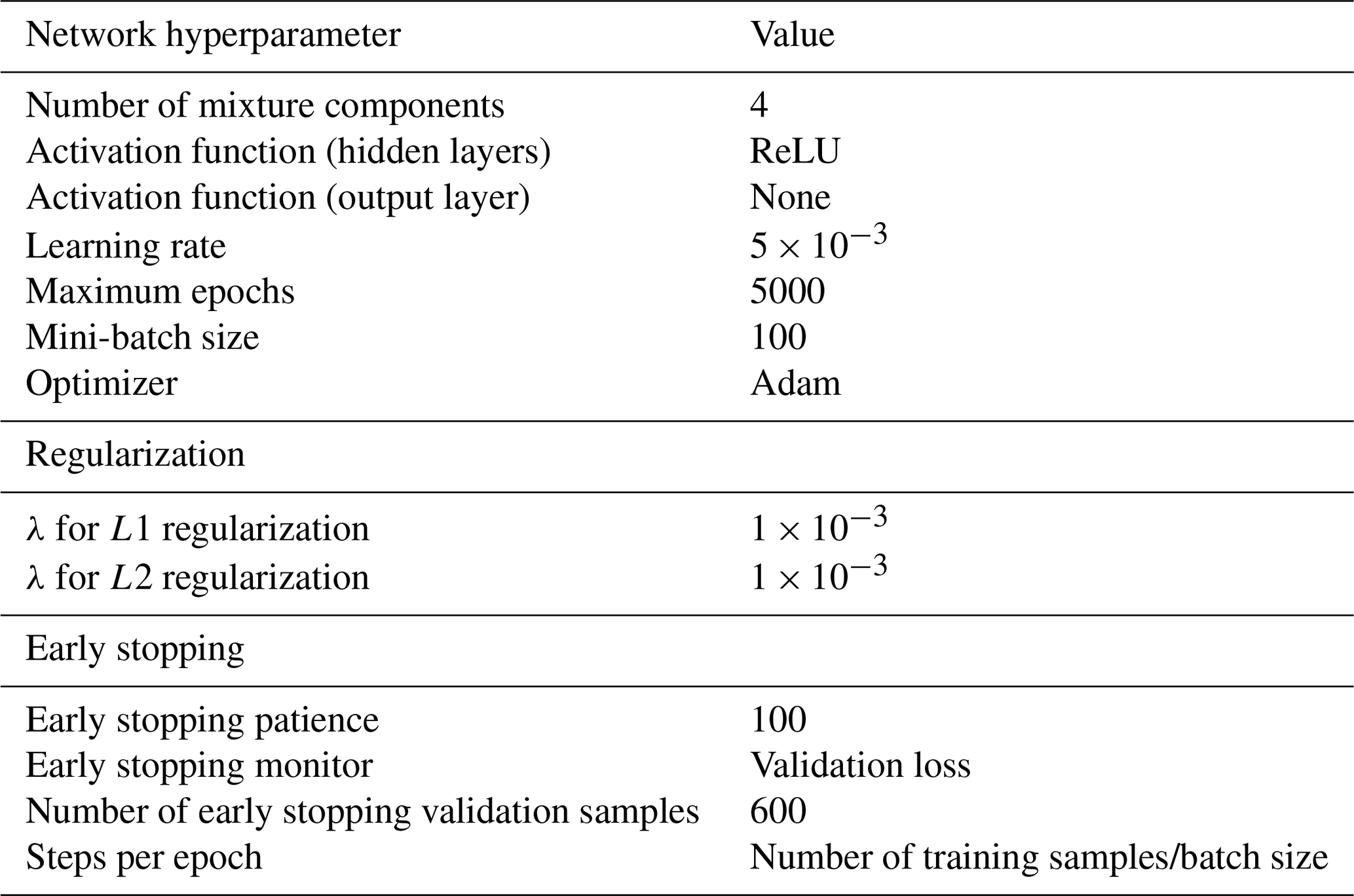
The derivative of the error function is calculated at the output layer and is back-propagated to obtain its gradient with respect to the network weights. The values of the network parameters are adjusted to minimize the error function using a gradient descent optimization. This study uses the Adam optimizer (Kingma and Ba, 2017) to perform stochastic gradient descent. The model is initialized 10 times for any given case in order to choose the best initial conditions for the optimizer. The hidden layers in our network use the rectified linear unit (ReLU). The output layer of the network does not have an activation function; therefore, the outputs are just linear combinations of the inputs from the previous layer.

Minimizing the error function is an ill-posed problem, as there is a conflict between learning the function that fits the data perfectly and remaining robust under varying sets of training data. As the network size grows, the function space increases and the neural network tends to overfit. The MDN model training especially seemed susceptible to it. Among several ways to avoid overfitting (Montavon et al., 2012), in this study, we implemented a combination of early stopping (Yao et al., 2007) and L1 and L2 regularization (Ng, 2004).

We implement MDNs using the Python-based TensorFlow Probability library (Dillon et al., 2017), with the output layer represented as a mixture of Gaussians via TensorFlow's mixture normal distribution (TensorFlow, 2025). The main hyperparameters used in this study to train the models to obtain the results in Sect. 4 are summarized in Table 6. In subsequent sections, we test the performance of the MDN model with various architectures. The features and targets are scaled with the standard scaler before training.

Table 6 Summary of the network hyperparameters.

3.2 Accuracy metric

The qualitative assessment of the performance of the surrogate model is based on two criteria: the coefficient of determination (R²) and the Wasserstein distance ($d_{W_{\mathrm{2}}}$), as described hereafter.

3.2.1 Coefficient of determination R²

The coefficient of determination, also known as the R², is a common measure of the goodness of fit of a model. It is defined as

$$\begin{array}{}\text{(6)}& R^{\mathrm{2}}=\mathrm{1}-{\displaystyle \frac{\sum (y_i-{\widehat{y}}_i{)}^{\mathrm{2}}}{\sum (y_i-\stackrel{\mathrm{‾}}{y}{)}^{\mathrm{2}}}},\end{array}$$

where ${\widehat{y}}_i$ is the predicted output, y_i is the observed value, and $\stackrel{\mathrm{‾}}{y}$ is the mean of the observed values. R² is interpreted as the linear correlation between the predicted and observed values of the output vector. To assess the accuracy of the predicted conditional distribution of the response compared to the BHawC reference, we calculate the R² value for the mean and standard deviation of the conditional probability density functions (PDFs). These two quantities are derived empirically by obtaining 5000 samples from the surrogate-predicted conditional distribution and n_seeds seed (turbulence and wave) repetitions per test case.

3.2.2 Wasserstein distance

The Wasserstein metric is a distance function that compares the difference between the PDFs of two random variables. It is symmetric and non-negative, and it satisfies the triangle inequality, making it a proper distance metric. In the case of 1D distributions, the Wasserstein-2 distance between a reference empirical measure Y and predicted measure $\widehat{Y}$ is defined as (Villani, 2009; Peyré and Cuturi, 2019; Ramdas et al., 2015)

$$\begin{array}{}\text{(7)}& W_{\mathrm{2}}(Y,\widehat{Y})={\left(\underset{\mathrm{0}}{\overset{\mathrm{1}}{\int }}\left|F^{-\mathrm{1}}\right(t)-G^{-\mathrm{1}}(t){|}^{\mathrm{2}}\mathrm{d}t\right)}^{\mathrm{1}/\mathrm{2}},\end{array}$$

where F⁻¹ and G⁻¹ are the quantile functions of Y and $\widehat{Y}$, respectively. The individual quantile functions are obtained from the samples of the empirical distributions and then integrated. In this paper, we calculate the Wasserstein distance between the conditional distribution predicted for each sample ($\widehat{Y}$) and the conditional distribution obtained as a reference through seed repetitions in BHawC/OrcaFlex (Y). $\widehat{Y}$ consists of 5000 samples from the surrogate's estimate, and Y is obtained from n_seeds turbulence and wave seed repetitions in BHawC/OrcaFlex. The distance metric is normalized by the standard deviation of the reference conditional distribution, Y. Therefore, a value of $\frac{W_{\mathrm{2}}}{\mathit{\sigma }\left(Y\right)}=\mathrm{1}$ is the distance between a distribution with mean μ(Y), scale σ(Y), and a degenerate distribution with the same mean. We calculate the global performance of the model by averaging the normalized Wasserstein distance over n_test test samples as

$$\begin{array}{}\text{(8)}& d_{W_{\mathrm{2}}}={\mathbb{E}}_{n_{\mathrm{test}}}\left({\displaystyle \frac{W_{\mathrm{2}}}{\mathit{\sigma }\left(Y\right)}}\right).\end{array}$$

4 Results

This section is divided into three parts. The first part presents a convergence study on the number of training samples, highlighting the model's robustness and demonstrating a clear trade-off between the computational cost of data generation and the resulting accuracy. A related hyperparameter study to determine the network architecture is presented in Appendix C. The second part validates the performance of the surrogate on the test dataset. The validated model is used to make lifetime fatigue damage estimates on the wind turbine components in response to different site conditions in the third section.

4.1 Choice of training data size

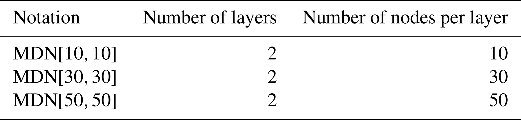
This section shows the convergence study with respect to the number of training samples for the tower bottom fore–aft DEL. It is assumed that the same architecture can be used to predict the remaining channels. Three networks for the mixture density networks are compared to test the robustness of the approach, as listed in Table 7. The MDNs contain four mixture elements. The rest of the hyperparameters are as specified in Table 6. In Fig. 9, at each N_train value, the models are trained on 25 different subsets of the total training data space to capture the sensitivity of the model's fit to the choice of the training samples. The boxes reflect the variation in the R² values as a result of the choice of training data points. The boxes extend between the data's first (Q₁) and third (Q₃) quartile, and the horizontal line across the box indicates the median. The difference between Q₁ and Q₃ defines the interquartile range (IQR). The upper whisker extends to the largest data values within 1.5 IQR above Q₃. The lower whisker, similarly, extends to the lowest data point within 1.5 IQR below Q₁. Outliers are visible as dots beyond the whisker boundaries. Figure 9a is the R² value obtained from predicting the mean of the conditional PDF of the tower bottom fore–aft DEL, averaged over the test dataset. The mean in the BHawC reference is calculated using 44 realizations of the wind and wave fields. The diminishing size of the IQR as the number of samples grows is a combination of the increasing robustness of the model and the smaller variability in the test samples as fewer untrained samples remain in the dataset.

Table 7 The MDN architectures considered for the convergence study.

MDN uses a neural network framework capable of inferring extremely complex underlying functions given sufficient data. In this case, MDN converges to consistent values of both R² of the conditional mean and $d_{W_{\mathrm{2}}}$ above 4250 samples. We also see that MDN estimates are closer to the ground truth with larger networks of 30 or 50 nodes per layer. The performance of MDN[30,30] and MDN[50,50] is almost identical in this region, indicating good model robustness with respect to the size of the layer.

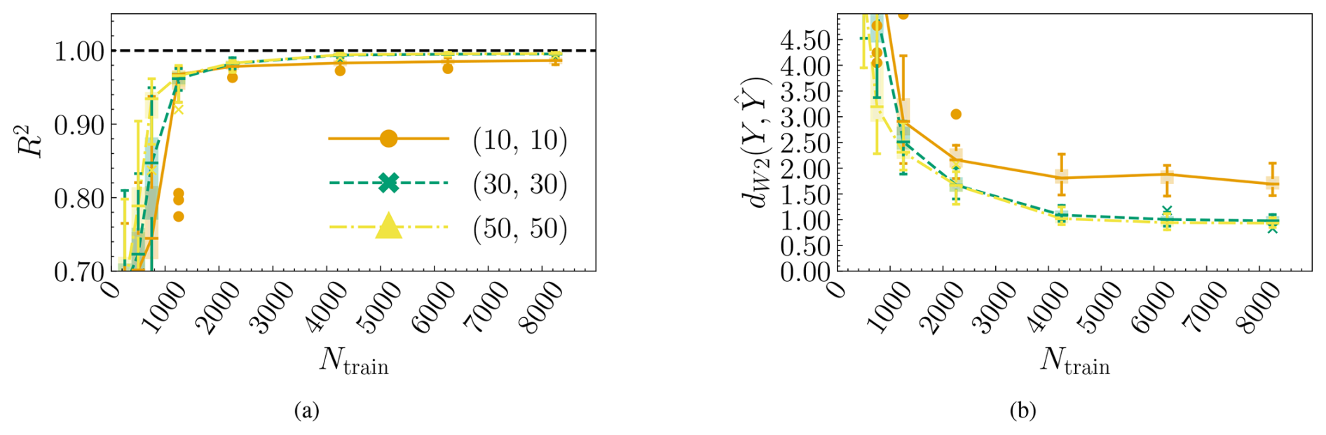
Figure 9 Convergence plots for the tower bottom fore–aft DEL channel. Panel (a) shows the convergence of the R² values of the predicted mean as a function of the number of training samples for three MDN architectures. Panel (b) shows the average normalized Wasserstein distance between the reference and predicted conditional PDFs as a function of the training samples.

Figure 9b shows the normalized 2-Wasserstein distance between the predicted and reference PDF. The Wasserstein distance quantifies the similarities between the predictions and the reference. It is, thus, a good indicator of whether or not the surrogate can correctly estimate the variation in the target resulting from a combination of epistemic and aleatoric sources. The predicted PDF is based on 5000 realizations from the estimated Gaussian mixture in MDN. The reference is based on n_seeds=44 BHawC/OrcaFlex realizations. Since 44 samples are insufficient to characterize the reference PDF fully, there is certainly an error associated with the $d_{W_{\mathrm{2}}}$ values; therefore, $d_{W_{\mathrm{2}}}$ cannot be expected to be zero in practice. Beyond 4250 samples, there is a small but marginal improvement in the $d_{W_{\mathrm{2}}}$ values from MDN[30, 30] and MDN[50, 50].

In conclusion, the two-layered MDN surrogates (MDN[30, 30] and MDN[50, 50]) reach convergence in terms of $d_{W_{\mathrm{2}}}$ at 4250 samples. For subsequent sections, the MDN models will be trained with a dataset of 8250 points, as this provides marginally better predictions with only a slight increase in model fitting cost.

The choice of the number of layers and nodes in the neural network, along with the number of mixture components, is based on a hyperparameter study, presented in Appendix C.

4.2 Surrogate model validation

In this section, the performance of the MDN model is evaluated for the load channels listed in Table 5, on the selected test dataset presented in Sect. 2.5.2. Based on studies in Sect. 4.1 and Appendix C, the values of hyperparameters used in training the models, in addition to Table 6, are listed in Table 8.

Table 8 List of hyperparameters used for training the MDN model for the final load prediction.

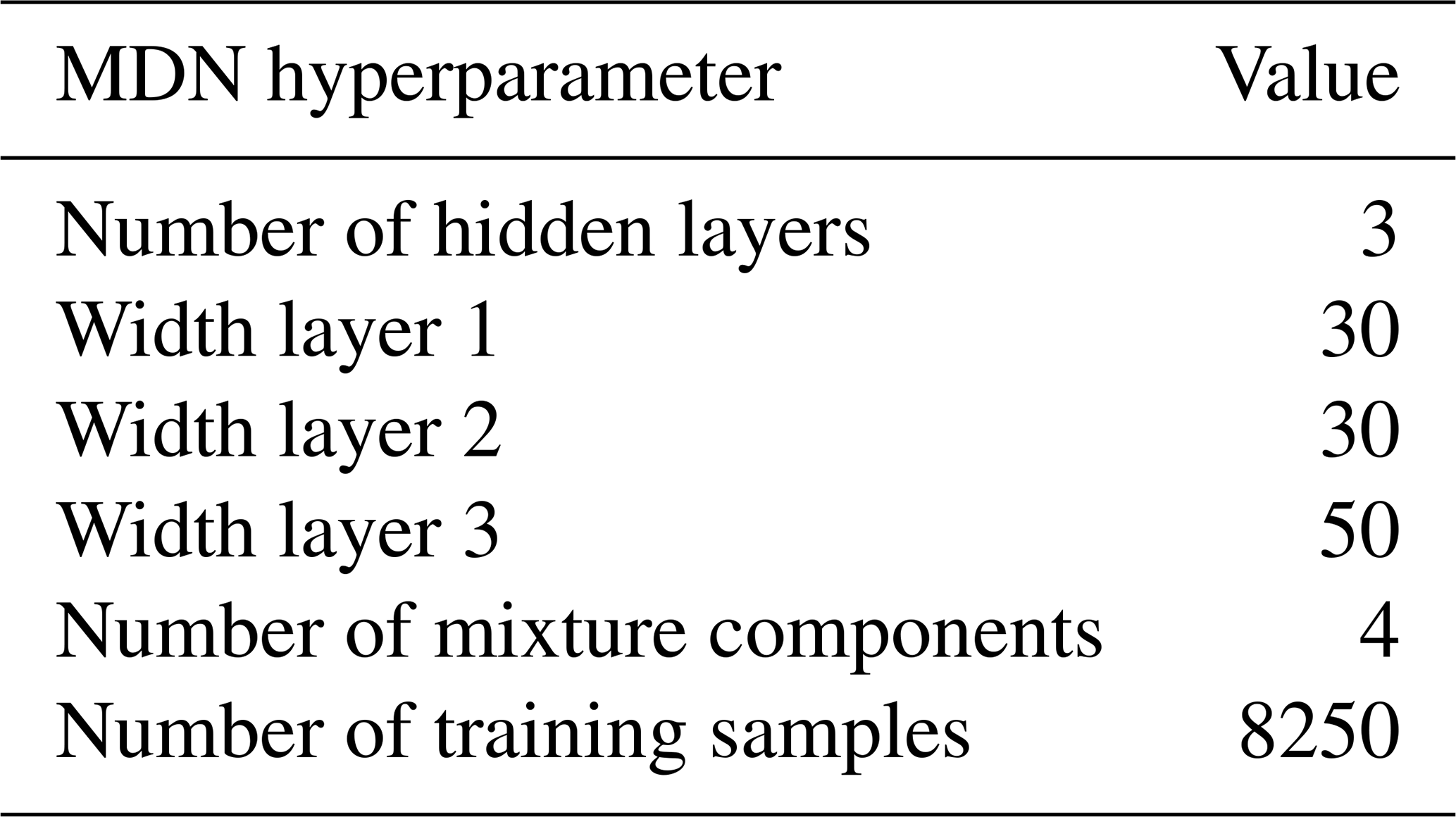
Table 9 provides a quantitative analysis of the model performance in terms of the average R² and $d_{W_{\mathrm{2}}}$ values. The conditional mean is accurately captured by the MDN model, with R² exceeding 0.99 on the test dataset. The goodness of fit on the conditional distribution is evaluated using $d_{W_{\mathrm{2}}}$. Lower $d_{W_{\mathrm{2}}}$ values indicate a smaller difference between the predicted and reference conditional distributions across the test database. As the $d_{W_{\mathrm{2}}}$ values are normalized by the local reference standard deviation, we can compare the performance of the models across different load channels. MDN's performance remains consistently good on the tower top and blade targets. The tower bottom channel shows a larger deviation in the $d_{W_{\mathrm{2}}}$ values, which is investigated further in Fig. 10.

Table 9 Quantitative analysis of the MDN model's predictions using $d_{W_{\mathrm{2}}}$ and R² as evaluation metrics.

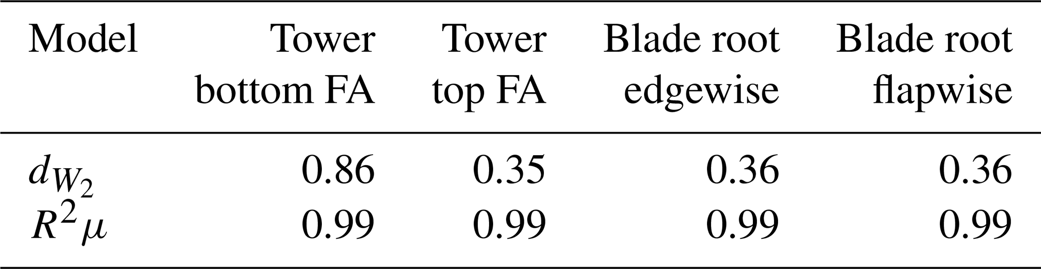
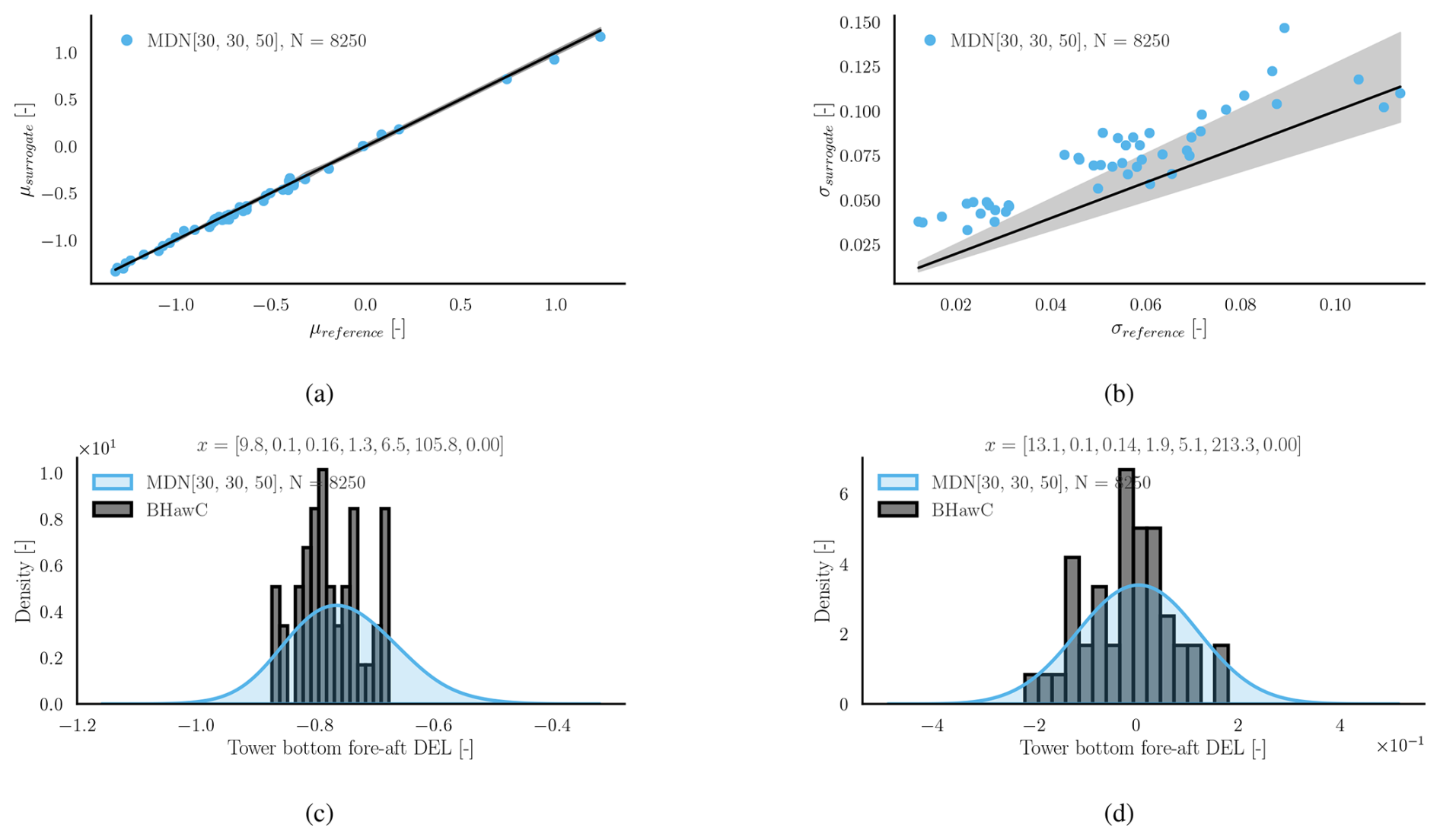
Figure 10 Load predictions using MDN for the tower bottom fore–aft DEL (normalized). Panel (a) shows the surrogate predicted conditional mean (μ_surrogate) at the test locations vs. the conditional mean calculated using BHawC (μ_reference). Panel (b) shows the predicted (σ_surrogate) and reference (σ_reference) standard deviations of the conditional PDF. Panels (c) and (d) compare the conditional PDF plots between the surrogate and the simulation at below-rated and near-rated conditions, respectively. The values in vector x denote [$U_{\mathrm{ref}},\mathit{\alpha },\mathrm{TI},H_{\mathrm{s}},T_{\mathrm{p}},W_{\mathrm{dir}},\mathrm{Yaw}$], with units specified in Table 4.

Figure 10 shows the statistics of the conditional distribution of the DEL variation at the tower bottom fore–aft direction. Since 44 seeds is a relatively small sample size to determine the true mean and standard deviation of the population, a gray area is highlighted in Fig. 10a and b to reflect the uncertainty in the reference values. For the mean, the 95 % confidence interval (CI_t) is calculated with the t distribution (Rouaud, 2013), assuming the response is normal. It is defined as

$$\begin{array}{}\text{(9)}& {\mathrm{CI}}_t={\mathit{\mu }}_{\mathrm{reference}}\pm t\cdot {\displaystyle \frac{{\mathit{\sigma }}_{\mathrm{reference}}}{\sqrt{n_{\mathrm{seeds}}}}},\end{array}$$

where μ_reference is the mean and σ_reference is the standard deviation calculated from the simulation samples. n_seeds=44 is the number of seeds with which the simulations were repeated. t is the t score for 95 % confidence, given n_seeds samples from a normally distributed population. The bounds are similarly calculated using the χ² distribution for the standard deviation. The bounds are asymmetric as the χ² distribution is skewed. χ_L and χ_R are based on 5 % and 95 % tails of the χ² distribution. The true standard deviation, σ, is expected to lie between the bounds,

$$\begin{array}{}\text{(10)}& \sqrt{{\displaystyle \frac{(n_{\mathrm{seeds}}-\mathrm{1})}{{\mathit{\chi }}_L^{\mathrm{2}}}}}{\mathit{\sigma }}_{\mathrm{reference}}\le \mathit{\sigma }\le \sqrt{{\displaystyle \frac{(n_{\mathrm{seeds}}-\mathrm{1})}{{\mathit{\chi }}_R^{\mathrm{2}}}}}{\mathit{\sigma }}_{\mathrm{reference}}.\end{array}$$

The individual PDFs are shown in Fig. 10 for two site conditions. The reference BHawC realizations are plotted as histograms overlaid with kernel density estimate (KDE) plots generated from 5000 samples from the conditional PDF predicted by the surrogate model. The estimates include two sources of uncertainty. The first is the epistemic uncertainty of inferring a function from limited data. The second is due to the irreducible noise term (aleatoric), which is a part of the observed stochastic process. The subsequent plots assume the standard deviation of the combined uncertainty.

Figure 10a shows the predicted conditional mean (μ_surrogate) of the normalized tower bottom fore–aft DEL as a function of the reference conditional mean (μ_reference) derived from BHawC/Orcaflex simulations. As already indicated in Table 9, the R² values are greater than 0.99 for MDN, indicating an excellent fit. Similarly, the standard deviation derived from the surrogates (σ_surrogate) is plotted against the ground truth reference (σ_reference) in Fig. 10b. Despite the slight over-prediction of the standard deviation, MDN is able to capture the heteroscedastic trend in the data. Figure 10c corresponds to a below-rated velocity of 9.8 m s⁻¹ and a wind–wave misalignment of 105^∘. Under these conditions, the BHawC reference is a short-tailed conditional PDF. Since MDN assumes a medium-tailed Gaussian mixture conditional, there is a tendency for the surrogate model to overestimate the standard deviation (Fig. 10b). The reason for the tower bottom fore–aft DELs to be restricted between a very small range resulting in such a short-tailed distribution is not obvious and demands a deeper investigation into the behavior of the tower structure and control laws, which is beyond the scope of this paper. A similar pattern is not observed in the other three load channels. Figure 10d corresponds to an example of a near-rated wind speed case, where the MDN predictions show a closer match to the reference conditional distribution.

A similar analysis is performed for the tower top fore–aft DEL channel in Fig. 11. The conditional standard deviation estimated from the MDN surrogate is within the error bounds of the small population assumption, indicating a very good fit.

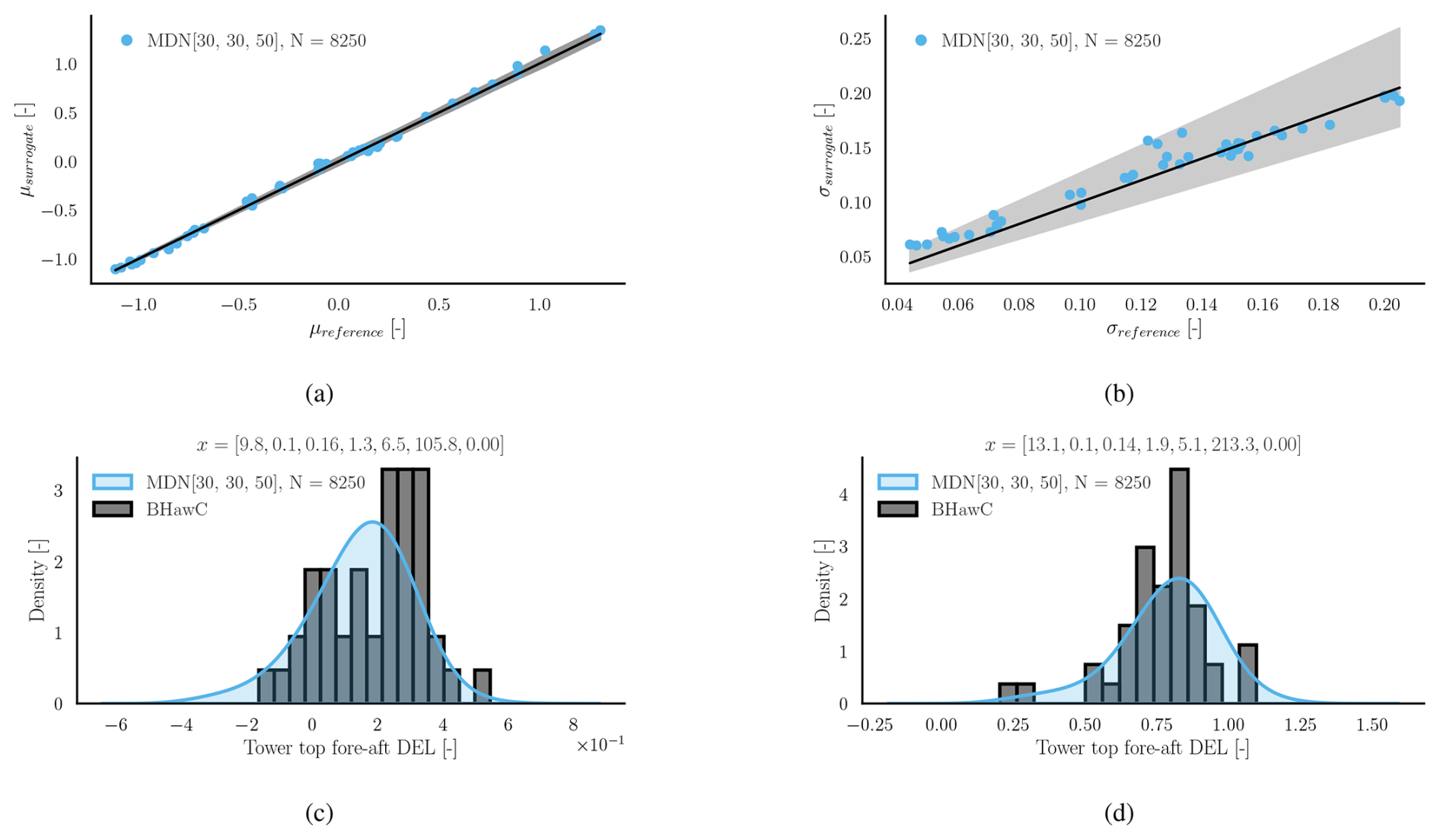
Figure 11 Load predictions using MDN for the tower top fore–aft DEL (normalized). Panel (a) shows the surrogate predicted conditional mean (μ_surrogate) at the test locations vs. the conditional mean calculated using BHawC (μ_reference). Panel (b) shows the predicted (σ_surrogate) and reference (σ_reference) standard deviations of the conditional PDF. Panels (c) and (d) compare the conditional PDF plots between the surrogate and the simulation at below-rated and near-rated conditions, respectively. The values in vector x denote [$U_{\mathrm{ref}},\mathit{\alpha },\mathrm{TI},H_{\mathrm{s}},T_{\mathrm{p}},W_{\mathrm{dir}},\mathrm{Yaw}$], with units specified in Table 4.

Figures 12 and 13 show the surrogate models' performance on the blade root flapwise and edgewise DEL, respectively. Similar to the tower top, the standard deviation and mean estimates from the MDN surrogate agree very well with the BHawC reference in both blade channels.

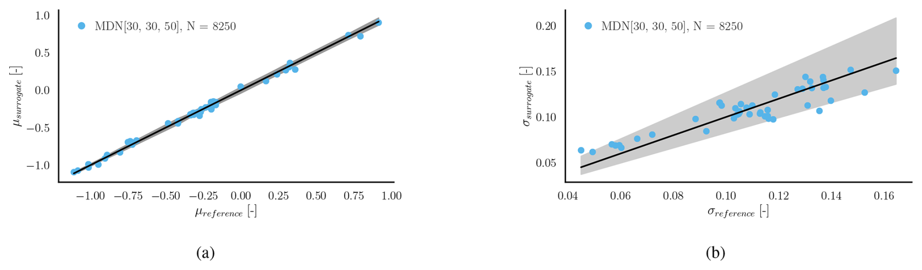
Figure 12 Load predictions using MDN for the blade root flapwise DEL (normalized). Panel (a) shows the surrogate predicted conditional mean at the test locations vs. the conditional mean calculated using BHawC. Panel (b) shows the predicted and reference standard deviations of the conditional PDF.

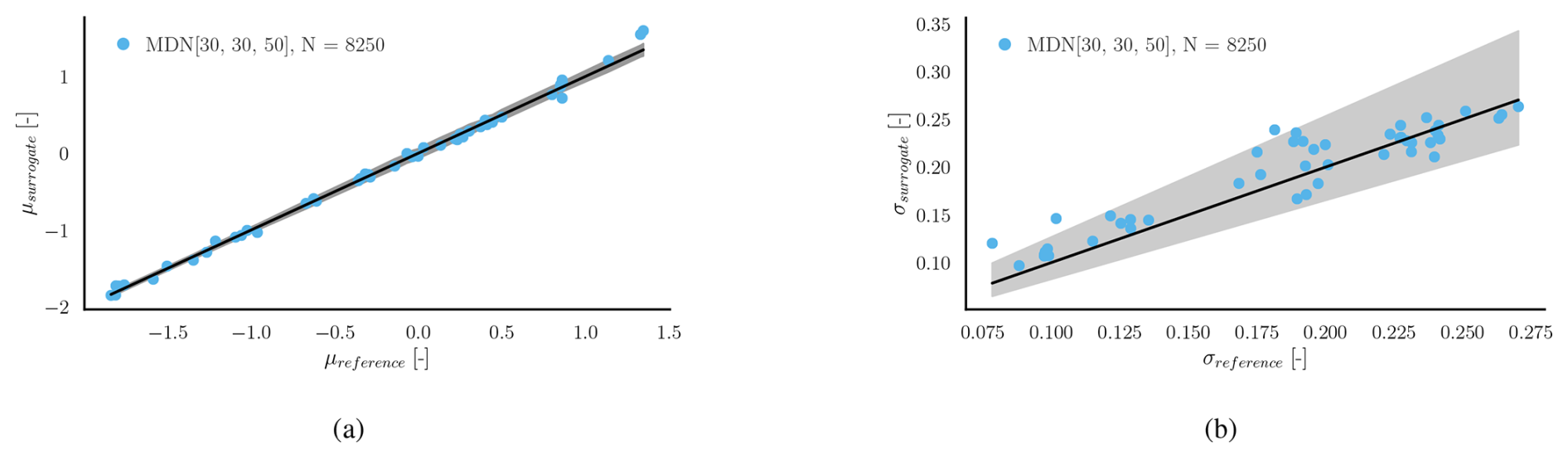
Figure 13 Load predictions using MDN for the blade root edgewise DEL (normalized). Panel (a) shows the surrogate predicted conditional mean at the test locations vs. the conditional mean calculated using BHawC. Panel (b) shows the predicted and reference standard deviations of the conditional PDF.

These results indicate that the surrogate model demonstrates a good level of reliability in accurately predicting the DELs with respect to the BHawC/OrcaFlex reference. Consequently, we assume that the model can be extended to other operating conditions without necessitating further verification.

4.3 Lifetime damage equivalent loads

The calculation of aggregated fatigue loads in onshore wind cases consists of binning the wind speed and scaling the loads at each bin by the probability of occurrence of the wind speed during the operating lifetime of the wind turbine. Floating wind turbine fatigue evaluations are more complex because, firstly, many more environmental parameters must be considered to characterize the site. Secondly, the bins need to be defined on a joint probability space. The process of choosing the right variables for the fatigue analysis and the size of the bins is not yet standardized and is a topic of ongoing research (Papi and Bianchini, 2024). With a fast surrogate model, however, it is possible to account for every single observation in the previous years, without the need to lump probabilities or limit the number of variables. The joint probabilities of the sea states are, therefore, automatically accounted for.

In this section, we use the validated surrogate model from Sect. 4.2 to make probabilistic estimates of the equivalent loads (M_eq) for 10 million reference load cycles on the floating wind turbine structure. The site data are obtained from the ERA5 database for four sites with an approximate water depth of 100 m, namely Sud de la Bretagne II, Emerald, Hywind Scotland, and HIP Atlantic (Table A1). Figure 14 provides an overview of the site conditions observed at the four selected sites. For simplicity, the foundation and mooring line design are assumed to be the same across the four sites. It is assumed that the difference in the load distributions between the design in use and the site-optimized foundation will not be significant. The ERA5 hourly conditions are converted to 10 min inputs by repeating each set of values six times. An alternative approach could be to draw the 10 min values from a normal distribution with the hourly values as the mean and an assumed standard deviation. The observations below cut-in and above the cut-out wind speed are excluded from the calculations. The site data consist of the average wind speed at 100 m, the significant wave height, the peak spectral period, the wind–wave misalignment (converted to wave direction in OrcaFlex coordinates), and the shear exponent. The yaw misalignment values are sampled from a normal distribution with zero mean and a standard deviation of 2°. The turbulence intensity is calculated for each case based on the wind speed, assuming the IEC 61400-1 turbulence class C classification.

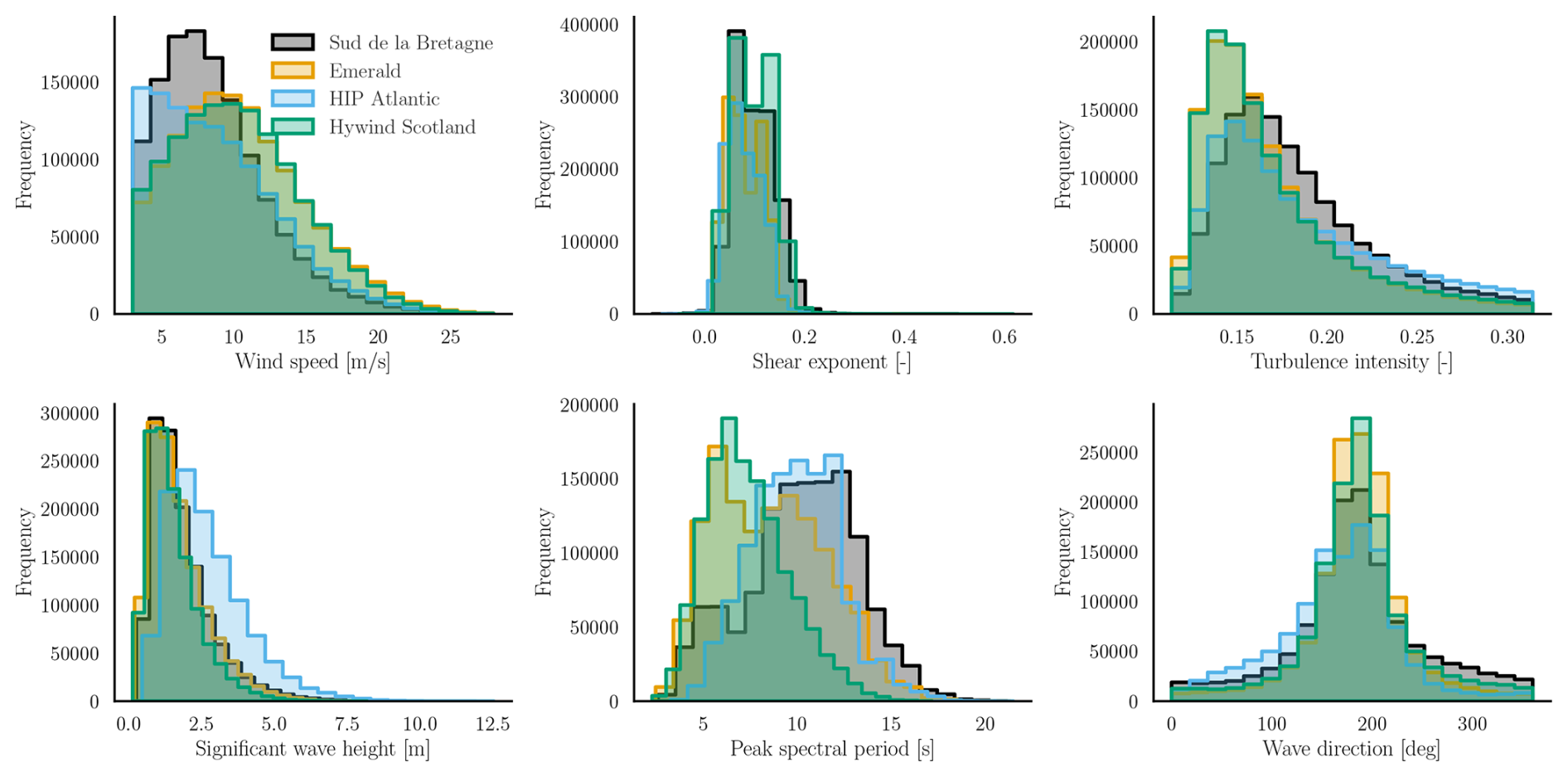
Figure 14 Comparison of the site conditions at the four floating wind sites considered in this study (Table A1).

The value M_eq represents the cyclic load amplitude which produces the equivalent lifetime damage given n_eq cycles of oscillation over L=25 years. In Eq. (11), M_i is the DEL for the ith 10 min of operation, and n_ref is the reference number of cycles per 10 min, set to 600. m is the Wöhler coefficient, with part-specific values listed in Sect. 2.3. n_L is the number of 10 min periods in L years. The loads do not have to be scaled, as the probability of occurrence of each condition is equal. Since the surrogate has been validated in previous sections, we assume here that its predictions are accurate, and we can treat each M_i as a probabilistic output from the MDN model. From each M_i PDF, we draw 500 samples, resulting in a probabilistic estimation of M_eq. M_eq is defined as

$$\begin{array}{}\text{(11)}& M_{\mathrm{eq}}={\left({\displaystyle \frac{n_{\mathrm{ref}}}{n_{\mathrm{eq}}}}\sum ^{n_L}{M}_i^m\right)}^{\mathrm{1}/m},\end{array}$$

where n_eq is 10⁶ and n_ref is fixed to 600 oscillations per 10 min period. The probabilistic M_eq value can be further used to calculate the stress reserve factor when re-designing the tower or to calculate the fatigue damage during the structure's operating lifetime.

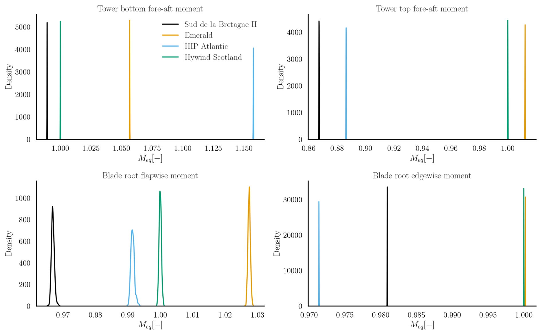
Figure 15 The 25-year normalized M_eq calculated for four sites at the tower bottom fore–aft direction (top-left), tower top fore–aft (top-right), blade root flapwise (bottom-left), and blade root edgewise (bottom-right) channels. The mean M_eq obtained at the Hywind Scotland site is used as the reference to normalize the loads at the remaining locations.

Figure 15 shows the kernel density estimate of the normalized M_eq values from the surrogate for the four selected sites. M_eq has been normalized by the average of the predicted M_eq values at the Hywind Scotland site for every channel. Firstly, it is interesting to note that the uncertainty in M_eq at each site is very small compared to the mean. This aligns with the law of large numbers, which states that, for M_i with a mean μ and variance σ², the standard deviation of the average of the distribution of (∑M_i) decreases as $\mathit{\sigma }/\sqrt{n_L}$. Since n_L is in the order of 10⁶, the standard deviation becomes extremely small as we get closer to the true mean. Even though the effect of M_i being raised to the power of m means that any variability in the sum is amplified, subsequently taking the mth root has the opposite, damping effect. Therefore, the effect of the outliers is essentially nullified due to the averaging. It is important to note that this study considers only the statistical uncertainty arising from stochastic input sources. In practice, other sources of uncertainty may contribute to the analysis (IEC, 2024b). For example, uncertainties related to the underlying joint distribution of site conditions represent another significant source of variability. Including these additional sources of uncertainties may introduce bias in the long-term mean, which is reflected as an uncertainty in the aggregated statistics of the outputs.

Secondly, the loads on different channels do not scale uniformly across sites. At the HIP Atlantic site, for instance, the cumulative tower bottom fore–aft moment is the highest, as shown in Fig. 15. This is primarily due to the influence of the significant wave height, which is expected to have a larger impact on the tower bottom fatigue (Singh et al., 2024c; Wiley et al., 2023; Edwards et al., 2023). The marginal distribution of significant wave height at this site shows a higher probability of larger waves compared to other locations, supporting the observed increase in tower bottom loads.

The distributions of wind speed, turbulence intensity, and significant wave height at the Emerald and Hywind Scotland sites (Fig. 14) are nearly identical. This results in comparable tower top fore–aft and blade root edgewise damage. However, there remains a significant difference in blade root flapwise fatigue accumulation. This result is surprising, given that the loads at this location are primarily wind-driven. Nevertheless, it underscores the complexity of fatigue damage accumulation, which can yield different outcomes with minor variations in site conditions even with respect to non-dominant variables.

5 Conclusions

5.1 Summary

This paper presents a framework to develop probabilistic surrogate models for predicting floating offshore wind turbine fatigue loads for site analysis. The surrogate maps the environmental conditions from potential farm sites to the 10 min damage equivalent loads experienced by a spar-type floating wind turbine. The main advantage of using probabilistic surrogates for this application is the ability to estimate conditional statistics with high accuracy to account for the statistical uncertainty resulting from the stochastic site conditions while minimizing the computational cost of training by avoiding seed repetitions. Based on the reanalysis data from the ERA5 database for several comparable floating sites, the surrogate model is used to propagate the statistical uncertainties to the 25-year fatigue loads on the wind turbine.

In this study, the analysis is performed on a spar buoy floating foundation based on a modified Hywind Scotland 6 MW wind turbine. The damage equivalent loads are considered on critical locations on the tower and blades and are calculated using a coupled implementation of BHawC/OrcaFlex for training and validating the surrogate. The features characterizing a floating farm site and the appropriate ranges are defined. The probabilistic model considered in this study is the mixture density network, as it is flexible, robust, and interpretable and has performed well for fixed-bottom load emulation in the literature.

Since MDN is based on a neural network parametrization, several hyperparameters require tuning prior to training. Therefore, a hyperparameter study is performed to find the appropriate neural network layout and the minimum number of training samples required to reach a high accuracy in terms of R²μ and $d_{W_{\mathrm{2}}}$. The conditional distribution predicted by the chosen model is validated on a set of 47 operating conditions, each simulated with 44 random seeds in BHawC/Orcaflex to obtain a reference conditional distribution for each test case. The R² value for estimating the conditional mean is >0.99 on all channels with the surrogate, indicating an excellent fit. The standard deviation of the conditional distribution is over-predicted by the model in the case of the tower bottom fore–aft moment but within the range of uncertainty bounds for the tower top and blade root channels.

Finally, the validated surrogate model is used to make probabilistic estimates of the 25-year equivalent damage on the tower and blades for four different sites. Since the surrogate model is fast, load predictions can be made quickly on all observed site conditions without lumping or binning the sea states a priori. We demonstrate that surrogate models can be powerful tools for site analysis, especially for floating wind turbines, where the choice of variables and binning methods is still an open question. Additionally, using probabilistic surrogates like MDNs helps reduce bias in calculating the aggregate mean fatigue, as the conditional distributions are not always normally distributed.

5.2 Discussion and future work

This section provides a critical discussion of the study's results, along with practical considerations and limitations associated with the use of MDNs.

5.2.1 10 min conditional DEL prediction

Given the stochastic nature of the site conditions, it is natural to model the 10 min DEL response within a probabilistic framework. MDN is demonstrated in this study to be a reliable tool for modeling the conditional distribution of 10 min DELs on the spar buoy floating wind turbine's tower and blades. MDN predictions are shown to remain robust across different network architectures and numbers of mixture components. The conditional means of the DELs are predicted with high accuracy, achieving an R²=0.99. Additionally, the Wasserstein distance between the predicted and reference conditional distributions shows a strong match at the blade roots and tower top. However, at the tower bottom, the conditional standard deviation of the 10 min fore–aft DEL is consistently over-predicted. It is corroborated by the relatively larger normalized Wasserstein distance value, indicating a bigger difference between the reference and predicted PDFs. Two main factors contribute to this: (i) the reference BHawC distributions are not converged at all simulated test locations with 44 random seeds. The tails of some distributions are not developed, resulting in short-tailed distributions that the MDN cannot easily capture. (ii) The tower bottom fatigue is shown in the literature to have a stronger correlation to the hydrodynamic parameters, leading to higher noise in the data. As MDN is trained to minimize the negative log-likelihood, it is rewarded for predicting higher variance when there is less confidence.

5.2.2 Probabilistic lifetime DEL aggregation

The uncertainty in the aggregated lifetime fatigue loads due to stochastic inputs is found to be much smaller in scale compared to the mean. This results from summing the 10 min DELs over 1 million occurrences, effectively nullifying the impact of the outliers. The use of a probabilistic surrogate that correctly captures the conditional distribution is still useful, as it minimizes the aggregation of error in the final response.

5.2.3 Notes on mixture density networks

Mixture density networks, due to their flexibility in modeling the conditional response, are well suited for the problem of probabilistic load estimation. One big advantage of the method is the ease of implementation and robustness, as demonstrated in this paper. Compared to deterministic models that often assume a Gaussian response to determine the conditional mean, mixture models can account for skewness and multimodality and improve the mean estimates. This is especially important for quantities like DELs, which may have non-Gaussian, heteroscedastic variations. MDNs scale well and are cost-effective to train compared to models that use Bayesian inference or variational inference (Blei et al., 2017).

MDNs without regularization can result in overfitting. Therefore, in this study, both L1 and L2 regularization are implemented. Secondly, MDNs rely on a stochastic optimizer that is sensitive to the initialization of the model parameters. Hence, a 10-fold cross-validation is recommended to ensure the optimizer is not stuck on a false minimum. As seen in the tower bottom fore–aft channel, minimizing the negative log-likelihood can result in the over-prediction of the standard deviation of the conditional response when the underlying distribution is short-tailed. MDNs here are not restricted to strictly positive values; in some cases, the tails may also extend to negative values. A potential solution is to assume a lognormal distribution for the output. This can be done by directly predicting the parameters of a lognormal distribution during training or by transforming the output to a normal distribution before training.

5.2.4 Future work

Future studies could use such surrogates to identify optimal methods for grouping sea states in order to reduce the number of physics-based simulations required to achieve the same lifetime fatigue loads as using all observed site data. This type of analysis would be computationally impractical with an engineering tool, as it would require the performance of millions of simulations to establish a baseline reference. Surrogates offer an alternative for reducing the computational demands while maintaining accuracy. Surrogate models can also be used in this context to isolate combinations of sea states that produce the highest fatigue on the wind turbine structure. Furthermore, it is interesting to include other sources of uncertainty in the analysis of loads, such as introducing an uncertainty on the parameters defining the joint distribution of the site conditions. Once trained, probabilistic surrogate models can be used to propagate the different uncertainty sources to the loads to study the combined effect without additional costs. This approach opens new opportunities for integrating reliability-based decision-making into the design process.

Appendix A: ERA5 locations used for defining feature ranges

Table A1 lists the locations used for defining the feature ranges in Sect. 2. The data are downloaded from the years 1979 to 2020. The database consists of the hourly average wind speeds at 10 and 100 m, the significant wave height, the spectral peak period, and the wave direction. The shear law exponent is derived from the wind speed values assuming a power law profile for the atmospheric boundary layer.

(Creane et al., 2024)(Creane et al., 2024)(Creane et al., 2024)(Creane et al., 2024)(Equinor ASA, 2014)(Vigara et al., 2019)(Vigara et al., 2019)(Vigara et al., 2019)(Creane et al., 2024)(Creane et al., 2024; Wind, 2025)(Creane et al., 2024; ESB, 2025)(Creane et al., 2024)

Table A1 Description of the sites used for defining the feature ranges.

Appendix B: Feature bounds

B1 Significant wave height

The upper and lower limits for the significant wave height are defined as functions of the wind speed at hub height U_ref.

The upper limit is a quadratic function of the form

$$\begin{array}{}\text{(B1)}& H_{{\mathrm{s}}_{\mathrm{U}}}=-\mathrm{0.008}{U}_{\mathrm{ref}}^{\mathrm{2}}+\mathrm{0.45}{U}_{\mathrm{ref}}+\mathrm{5}.\end{array}$$

The lower limit is defined as

$$\begin{array}{}\text{(B2)}& H_{{\mathrm{s}}_{\mathrm{L}}}=\mathrm{0.719}{e}^{\left(\mathrm{0.0832}{U}_{\mathrm{ref}}\right)}-e^{\left(\mathrm{0.04}{U}_{\mathrm{ref}}\right)}.\end{array}$$

B2 Peak spectral period

The peak spectral period range is designed to be a function of the significant wave height (which is, in turn, a function of the wind speed at hub height). We define scaling functions A, B, and C as

$$\begin{array}{}\text{(B3)}& {\displaystyle }A=a_{\mathrm{1}}+a_{\mathrm{2}}{H}_s^{a_{\mathrm{3}}}\text{(B4)}& {\displaystyle }B=b_{\mathrm{1}}+b_{\mathrm{2}}{e}^{-b_{\mathrm{3}}{H}_{\mathrm{s}}}\text{(B5)}& {\displaystyle }C=c_{\mathrm{1}}+c_{\mathrm{2}}{e}^{-c_{\mathrm{3}}{H}_{\mathrm{s}}}.\end{array}$$

The scaling functions are used to define the upper bound $T_{{\mathrm{p}}_{\mathrm{U}}}$ and lower bound $T_{{\mathrm{p}}_{\mathrm{L}}}$ as

$$\begin{array}{}\text{(B6)}& {\displaystyle }{T}_{{\mathrm{p}}_{\mathit{\mu }}}=e^{(A+\mathrm{0.5}B)}\text{(B7)}& {\displaystyle }{T}_{{\mathrm{p}}_{\mathrm{L}}}=T_{{\mathrm{p}}_{\mathit{\mu }}}(\mathrm{1}-\mathrm{3}\times \sqrt{(e^B-\mathrm{1})})\text{(B8)}& {\displaystyle }{T}_{{\mathrm{p}}_{\mathrm{U}}}=T_{{\mathrm{p}}_{\mathit{\mu }}}(\mathrm{1}+\mathrm{3}\times \sqrt{(e^C-\mathrm{1})}).\end{array}$$

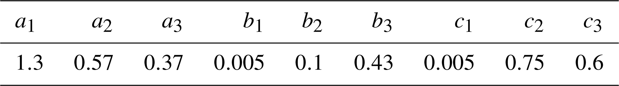
The coefficients used to fit the curve in this study are listed in Table B1.

Table B1 Tuning coefficients for defining the range functions for the spectral wave period.

Appendix C: Choice of hyperparameters

C1 Number of layers and nodes

Large networks are better at capturing complex expressions in data but are susceptible to overfitting with a small training set. The objectives of this study are, firstly, to observe the robustness of the model relative to the number of network parameters for a particular training data size and, secondly, to choose a network architecture suitable for the rest of the study.

A sensitivity study on the number of nodes and layers is performed in this section for a training dataset of 8250 samples. The number of mixture parameters is four in all cases, and the rest of the network hyperparameters are fixed to the values listed in Table 6. Networks with two, three, and four layers with various widths are tested. The x axis in Fig. C1 lists the combinations of widths per layer evaluated in this study. The tower bottom fore–aft DEL channel is chosen for this study.

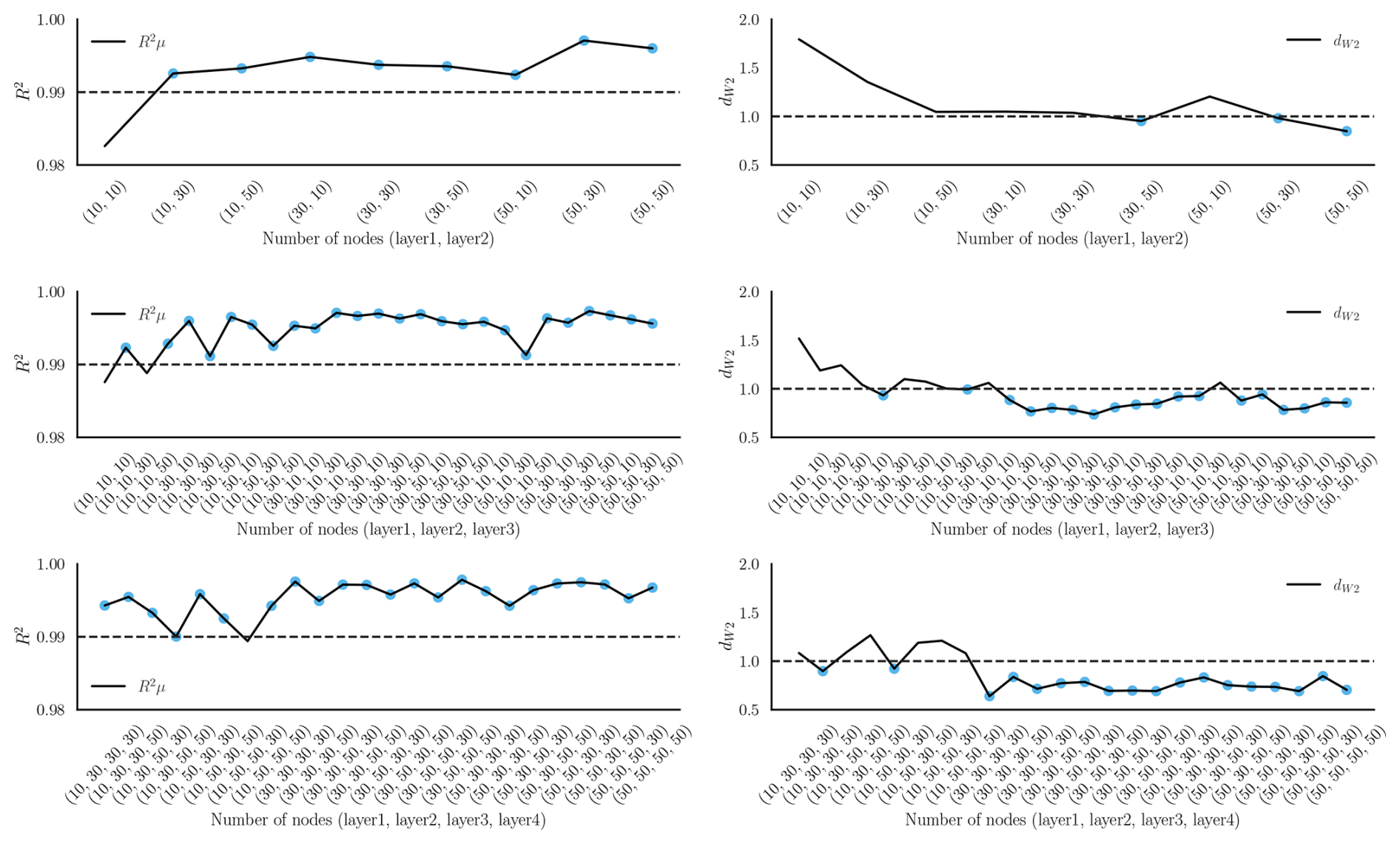
Figure C1 Study on the network architecture. The x axis reflects the number of nodes per layer. The rows correspond to two-, three-, and four-layer networks. The left column shows the R² value for the mean of the conditional PDF of the tower bottom fore–aft DEL channel. The dashed line corresponds to an R² value of 0.99. The right column plots the $d_{W_{\mathrm{2}}}$ values for the same channel with the dashed line corresponding to a $d_{W_{\mathrm{2}}}$ value of 1.

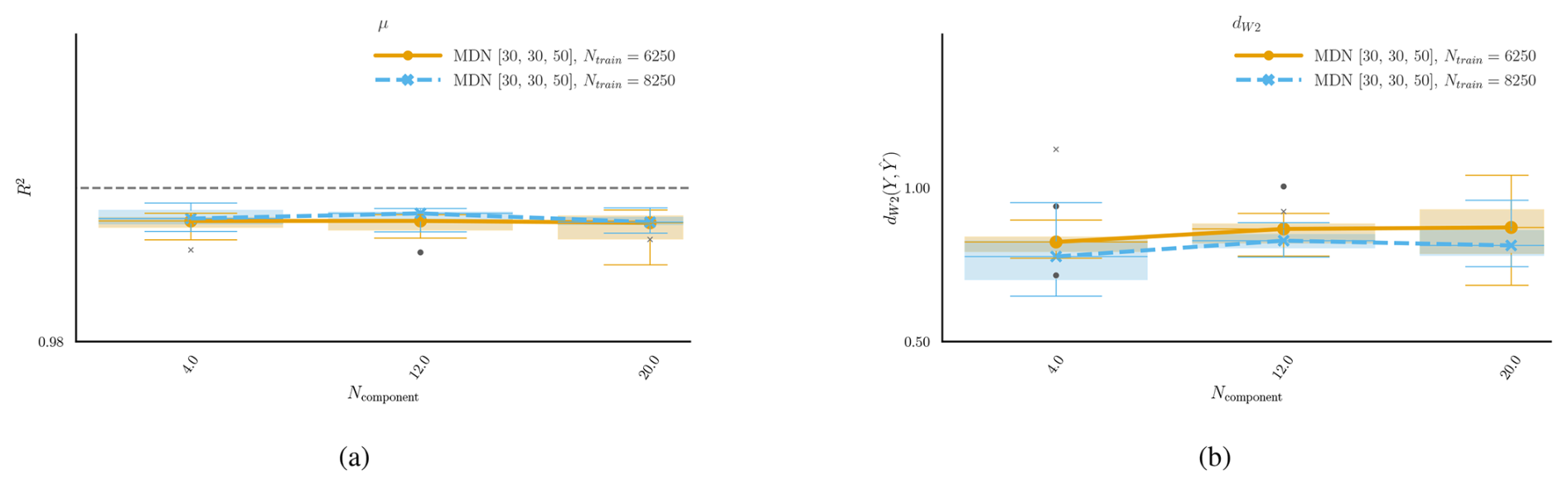
Figure C2 Sensitivity of the MDN surrogate to the number of mixture components (N_component) for the tower bottom fore–aft DEL. Panel (a) shows the R² values for the predicted mean. Panel (b) indicates the average normalized $d_{W_{\mathrm{2}}}$ for the predicted conditional PDF.

The R² values of the DEL are notably good for the architectures tested, indicating good model robustness. The main differences observed are in $d_{W_{\mathrm{2}}}$, where the large three- or four-layer networks are generally better at capturing the complete conditional PDF. For the remainder of this study, we chose a three-layer network with 30 nodes in layer 1, 30 nodes in layer 2, and 50 nodes in layer 3 in combination with 8250 training samples.

C2 Number of mixture elements

The number of Gaussian distributions in the mixture controls the complexity of the predicted conditional PDF. However, a large number of unnecessary mixture elements add redundancy and increase the computational complexity of the surrogate. In this section, we use 6250 and 8250 training samples with a three-layer architecture width = (30, 30, 50) and test the performance of 4, 12, and 20 mixture elements on the tower bottom fore–aft DEL channel.

The number of components does not affect the estimation of the tower bottom fore–aft DEL mean. A slight improvement can be seen in Fig. C2b with four components. The model, therefore, appears to be robust regarding the choice of the number of mixture components. In other words, it does not necessarily benefit from a large set of mixture components. MDN models in the remainder of the study are trained with four kernels.