Optimal allocation of 30 GW offshore wind power in the Norwegian economic zone

The Norwegian Government aims to install offshore wind power with a total capacity of 30 GW by 2040, and the Norwegian Water Resources and Energy Directorate has suggested 20 candidate regions. We show that the potential for reducing overall power production variance across these regions is high using modern portfolio theory and the hourly and spatially rich reanalysis NORA3 Wind Power data set (NORA3-WP). The geographical diversification effect is demonstrated under various relevant scenarios, including a sequential build-out scenario with a fully connected Norwegian power grid assumption. By considering 20 alternative regions selected using a recently developed suitability score, we further illustrate that the diversification effect is robust to location changes.

1 Introduction

Policymakers, environmental organizations, industry and researchers portray offshore wind power as a vital energy source to meet the increasing demand for clean, renewable energy as the world transitions from fossil fuels. Norway has a large and largely unexploited potential for offshore wind power production (Bosch et al., 2018). The Norwegian Government has presented an ambitious development plan, called 30by40, of continuously opening offshore areas for large-scale wind power deployment, sufficient for 30 GW installed capacity by 2040 (Norwegian Government, 2022). Theoretically, having only one wind farm with 30 GW of installed capacity would occupy 9400 km², corresponding to a square with sides of 97 km (Solbrekke, 2022). However, distributing wind farms across a larger geographic area could stabilize the instantaneous power production (Solbrekke et al., 2020; St.Martin et al., 2015). If there is little wind in one area, this can be compensated by windy conditions somewhere else. This effect is analogous to diversification in financial portfolio selection problems using modern portfolio theory (Markowitz, 1952). Thus, we consider the distribution of wind farms as an optimization problem, where we aim to maximize power production while minimizing its variance. In the context of opening several areas for offshore wind power deployment, where the instantaneous wind resources are more or less dependent, it is crucial to first determine the location of potential wind farms. We then apply modern portfolio theory to determine the relative sizes of the wind farms to obtain the best tradeoff between power output and stability. Our objective is to find the portfolio that minimizes the variance given a specific expected power output. We advance the current literature by introducing a new set of cardinality constraints and a novel sequential build-out routine. Modern portfolio theory has a long history in financial portfolio selection, where the weights represent how large a portion of the total investment one should invest in different stocks, bonds, or funds. In a wind farm portfolio, the weights correspond to the proportion of the total number of wind turbines potentially installed at each wind farm location.

The Norwegian (exclusive) economic zone (NEZ) is extensive, and not all areas are suitable for installing turbines. In most areas, the sea depth is too large for anchoring wind turbines to the sea floor at an acceptable cost. Some areas are known to be spawning grounds for fish, while other areas may be too close to other offshore installations, such as oil and gas platforms. In this paper, we only consider locations that are suitable for the installation of offshore wind turbines. We achieve this by using two different approaches when selecting suitable candidate sites. Our first set of candidate locations was suggested by the Norwegian Water Resources and Energy Directorate (NVE). The NVE suggests 20 areas in the NEZ for further consideration in a subsequent impact assessment. Our second set of candidate locations is based on the study by Solbrekke and Sorteberg (2023), who use a multicriteria decision analysis to point out suitable and robust offshore areas for wind power deployment.

Markowitz's modern portfolio theory (Markowitz, 1952) has been applied to wind power production several times in the literature. Drake and Hubacek (2007) study the geographic diversification effect of wind farm portfolios in the United Kingdom by comparing a portfolio of 2.7 GW in one location to one where the same energy is distributed over four locations. They find a reduction of 36 % in the standard deviation of instantaneous wind power production. Roques et al. (2010) consider total wind production data from five European countries (Spain, France, Germany, Denmark and Austria) and apply modern portfolio theory to minimize variance, in a theoretical unconstrained portfolio as well as a portfolio in which national wind resource potential and transmission constraints are taken into account. Rombauts et al. (2011) build on the work of Roques et al. (2010), but instead of using aggregated data by country, they apply portfolio theory on simulated data from different locations within each country. They also model cross-country transmission constraints more explicitly. With case studies from the United States, Degeilh and Singh (2011) propose a general planning method to minimize the variance of aggregated wind power output by optimally distributing turbines over a preselected number of potential sites, Novacheck and Johnson (2017) study the potential for diversification of wind power variability in the Midwest, and Costa-Silva et al. (2017) use modern portfolio theory with 4 re-balancing strategies on 11 hypothetical offshore wind farms off the US East Coast. Hjelmeland and Nøland (2023) analyze the correlation structure between potential Norwegian offshore wind resources and existing resources in neighboring countries concerning potential price effects. More recently, Tejeda et al. (2018) employed the ERA-Interim wind resource reanalysis data to minimize the variability of aggregated wind farm production over a 0.25×0.25° grid of onshore Europe (EU-28) and a selection of offshore grid cells.

In this study, we use the high-resolution wind power reanalysis NORA3-WP (see Sect. 2.1), which is a dynamic downscaling of the state-of-the-art reanalysis ERA5 (Hersbach et al., 2020). Comparing NORA3-WP to the data set used by Tejeda et al. (2018), NORA3-WP has a higher temporal resolution (hourly versus 6-hourly) and a more extended history (24 years versus 10 years). Furthermore, the analysis by Tejeda et al. (2018) includes most of the European continent, while we focus exclusively on sites in the NEZ suitable for offshore wind power installations. Instead of placing wind power by grid cell (Tejeda et al., 2018), we find the optimal number of turbines on a wind farm unit represented by the wind resources from one grid cell in NORA3-WP. Our study, therefore, builds naturally on recent developments in the identification of suitable locations for wind power generation (Solbrekke and Sorteberg, 2023) and methodology for distributing resources between them (Tejeda et al., 2018). We develop the procedure for wind power distribution further by incorporating the Norwegian Government's sequential development plan, 30by40, and introducing a constraint on the maximum number of wind farms (see Sect. 3).

The structure of this paper is as follows. We present the NORA3-WP data in Sect. 2.1. We then present the NVE candidate locations and the Solbrekke and Sorteberg (2023) counterpart. In Sect. 3, we present Markowitz's portfolio theory with particular adaptations specific to the wind power problem. We set up five cases with varying constraints and build-out strategies. The optimal portfolios are presented and discussed in Sect. 4. We then give some concluding remarks in Sect. 5.

2 Data

2.1 NORA3-WP

The backbone of this study is the new wind resource and wind power data set NORA3-WP constructed by Solbrekke and Sorteberg (2022). It is based on the 3 km Norwegian reanalysis data (NORA3), which is the most recent high-resolution data archive from the Norwegian Meteorological Institute (Haakenstad et al., 2021), generated by a dynamical downscaling of ERA5 (Hersbach et al., 2020). Solbrekke et al. (2021a) and Haakenstad et al. (2021) carry out a validation of NORA3 against observations, together with a comparison of NORA3 to the host data set ERA5. These studies conclude that NORA3 is consistently closer to the observed wind speed compared to ERA5, especially over land, where the topography is complex, and for high wind speeds. Cheynet et al. (2022) compare NORA3 to the New European Wind Atlas. Both data sets are found to provide reliable estimates of the mean wind speed, but NORA3 shows slightly better performance for the mean wind speed in terms of root-mean-square error, bias, earth mover's distance and Pearson correlation coefficient (Cheynet et al., 2022).

NORA3-WP covers the North Sea, the Norwegian Sea, the Baltic Sea and parts of the Barents Sea in a 3 km × 3 km horizontal grid. NORA3-WP contains climatological data on a monthly timescale from 1996 to 2019, providing 7 wind resources and 18 wind power-related variables for 3 selected turbines with different power ratings, turbine diameters and hub heights. The underlying hourly wind speed and wind power data are also available on the same spatial scale. For more details on the data, see Solbrekke and Sorteberg (2022).

In this study, we use the hourly wind power data, calculated using the 15 MW reference turbine from the International Energy Agency, IEA-15 MW (Gaertner et al., 2020), which is the largest among the three turbines covered by NORA3-WP. IEA-15 MW has a rated power of 15 MW, a hub height of 150 m and a rotor diameter of 240 m. If the wind speed is below 3.0 m s⁻¹ or above 25 m s⁻¹, the power production is zero due to internal friction and sheltering purposes, respectively. If the wind speed is between 3.0 and 10.59 m s⁻¹, the power production is proportional to the wind speed cubed. Lastly, if the wind speed lies between 10.59 and 25 m s⁻¹, the turbine produces its rated power.

Using the IEA-15 MW turbine in our analysis implies that installing 30 GW of offshore wind power corresponds to building 2000 turbines. From the NORA3-WP data, we extract hourly time series from the grid cells closest to the center of the NVE regions described in the next section and the actual grid cells from the Solbrekke and Sorteberg (2023) selected locations in the following section. We calculate the mean capacity factor, i.e., the average production as a percentage of rated power, and the covariance matrix describing the linear dependence between the different locations. This mean vector and covariance matrix is then used in the portfolio optimization described in Sect. 3. Since the capacity factor is a relative measure in [0,1], we report it as a percentage. Note that the standard deviation of a capacity factor is then measured in percentage points (pp).

2.2 Norwegian Water Resources and Energy Directorate (2023) candidate locations

The Norwegian Water Resources and Energy Directorate (NVE) led a group with members from different state agencies (the Norwegian Petroleum Directorate, Directorate of Fisheries, the Norwegian Environment Agency, the Norwegian Coastal Administration and the Norwegian Defence Estates Agency) with a mandate from the Norwegian Ministry of Petroleum and Energy to identify suitable locations for offshore wind farms that have few conflicting interests (Norwegian Water Resources and Energy Directorate, 2023). The group of directorates identified 20 regions suitable for wind power (see shaded areas in Fig. 1d). In September 2023, the Norwegian Government instructed the NVE to start an impact assessment on 3 of these 20 areas: Vestavind B, Vestavind F and Sørvest F (Norwegian Government, 2023). Parts of Sørvest F and Vestavind F were considered previously for wind power production under the names Sørlige Nordsjø 2 (SN2) and Utsira Nord (UN), respectively. SN2 and UN were identified in an earlier report by the NVE (Norwegian Water Resources and Energy Directorate, 2012), and it has been decided to allocate areas for 1500 MW at each location to start with. We will, therefore, make sure these are in both candidate sets and use the names SN2 and UN for the corresponding areas in both sets. The suggested regions from 2012 were also used in the analysis by Hjelmeland and Nøland (2023). The NVE used a tool called “Marine Resources Tools”, or MaRS, for selecting the newest areas (The Crown Estate, 2019). This is essentially a suitability analysis that excludes certain areas due to input from the interest group members.

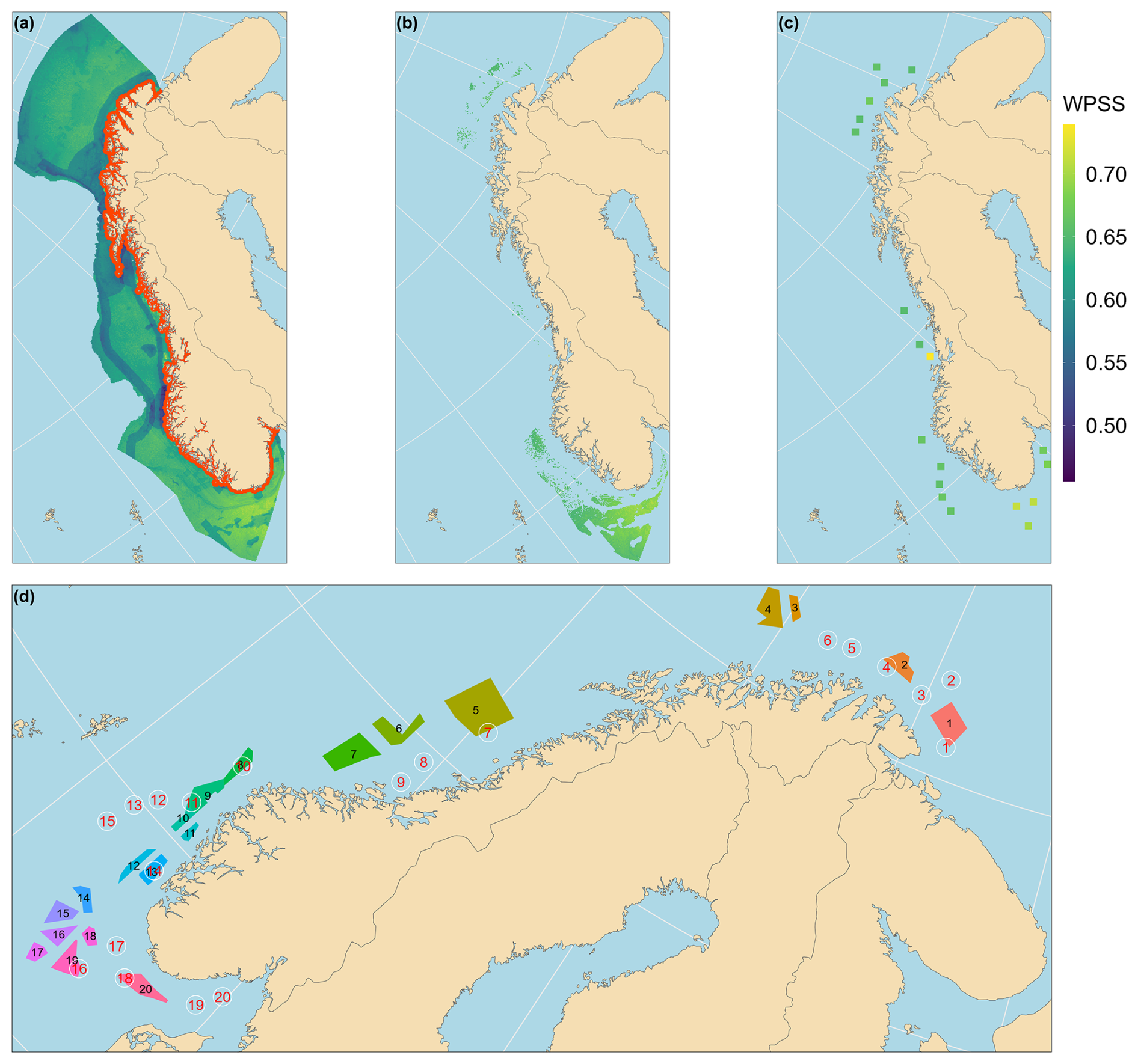
Figure 1 (a) All locations in the NEZ are colored by the wind power baseline suitability score (WPSS). (b) Locations that are in the top 25 % WPSS in all suitability perspectives are colored according to baseline. (c) The 19 locations selected after running Algorithm 1. (d) The 19 locations chosen as potential wind farm sites with Utsira Nord added, numbered from 1 to 20 in red numbers with white circles around and the 20 NVE-suggested areas numbered from 1 to 20 as shaded areas with black ID numbers (see Table 1). Colors are only used to distinguish the regions.

The total area covered by the 20 regions suggested by the NVE is 54 867 km². The Norwegian Water Resources and Energy Directorate (2023) uses different capacity densities (3.5, 5 and 7.5 MW km⁻²) and different area utilization rates (33 %, 67 % and 100 %). We choose the lowest capacity density and a 100 % utilization rate for our study.¹ Using these parameters, we can calculate the maximum number of turbines per region by

$$\begin{array}{ll}{\displaystyle }& {\displaystyle }\text{potential installed capacity}=\text{area}\cdot \mathrm{3.5}{\text{ MW\hspace{0.17em}km}}^{-\mathrm{2}}\cdot \mathrm{100}\mathit{\%},\\ {\displaystyle }& {\displaystyle }\text{maximum NoT}=\lfloor {\displaystyle \frac{\text{potential installed capacity}}{\mathrm{15}\text{ MW}}}\rfloor ,\end{array}$$

where ⌊⋅⌋ means rounding down to the nearest integer, and NoT is the number of turbines. The area and resulting potential capacity and maximum number of turbines per region are given in Table 1. The coordinates in the table are the average of the corners of the regions. Using these parameters (3.5 MW km⁻² and 100 % utilization rate), the potential capacity of these regions is 192 GW or 12 802 turbines. If we instead had used the most optimistic parameters in the report (7.5 MW km⁻² and 100 % utilization rate), the numbers would be 412 GW and around 27 400 turbines. In the table, we have also included a maximum portfolio weight given a total of 2000 turbines, which is used as a constraint in the portfolio optimization presented in Sect. 3.

Table 1 The NVE-selected locations with coordinates and area. The potential installed capacity is calculated using a capacity density of 3.5 MW km² and 100 % area utilization rate. The maximum number of turbines (NoT) is based on 15 MW per turbine, and CF is the capacity factor. Note that the standard deviation (SD) is measured in percentage points (pp).

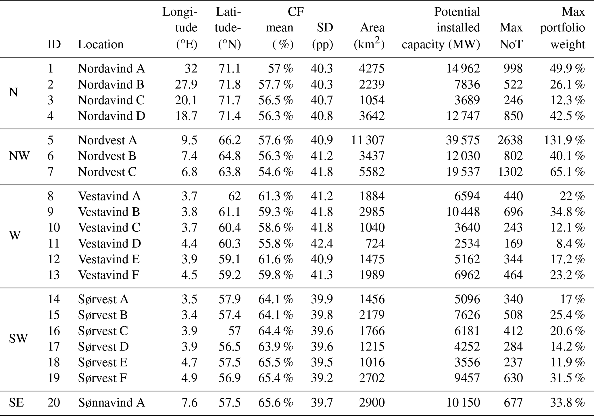
We have also included the average and standard deviation of the hourly capacity factor, estimated from the NORA3-WP data at the closest grid cell to the given coordinates in Table 1. The averages range from 54.6 % to 65.6 %, and the standard deviations range from 39.2 to 42.4 pp. The expected capacity factor for any portfolio based on these locations will fall in this range of means. We show below that the diversification effect reduces the standard deviation of the total hourly power production considerably.

We refer to these candidate locations as the NVE locations.

2.3 Candidate locations based on Solbrekke and Sorteberg (2023)

Solbrekke and Sorteberg (2023) constructed wind power suitability scores (WPSSs) for potential wind farm locations for the entire Norwegian economic zone (NEZ), taking into account many relevant factors like wind resources, techno-economic aspects, social acceptance, environmental considerations and met-ocean constraints such as wind and wave conditions. Solbrekke and Sorteberg (2023) exclude some grid cells due to, e.g., oil platforms or other obstacles, but areas are not excluded solely due to input from one interest group. Since the user must specify the importance of the different criteria, the WPSS is not an objective measure. To cope with the subjective criteria weights, Solbrekke and Sorteberg (2023) carried out a sensitivity analysis where the criteria importance was tuned according to distinct preferences of three actors: the investor, the environmentalist and the fisher. The result from Solbrekke and Sorteberg (2023) gives information about which NORA3-WP grid cells are most suited for wind power in the NEZ, and the sensitivity analysis reveals which of these are robust to changes in criteria importance.

To avoid some candidates very close to shore, we add a requirement that the offshore location should be at least 15 km from the nearest land mass and select locations with a WPSS above a certain percentile, α, from the baseline scenario and the three actors of Solbrekke and Sorteberg (2023). To be deemed a suitable location, all three actors and the baseline suitability score must agree that the location is among the top 100 α % of candidates, $\mathit{\alpha }\in (\mathrm{0},\mathrm{1})$. Thus, all candidate locations are grid points with the highest and most robust suitability scores.

Our goal is not to place each wind turbine precisely but, more generally, to place the wind farms. We allow one grid cell (3 × 3 km) to represent one wind farm and its surrounding area. Therefore, we do not want to include grid points too close to each other. If two points are within r km from each other, we select the one with the highest baseline WPSS. The algorithm for doing this is described below, in Algorithm 1. Two choices affect the number of candidate locations: the minimum distance between candidates r and the percentile of a WPSS α.

Algorithm 1 Algorithm of selecting candidate locations.

Let 𝒮 denote the set containing candidate locations. A priori, these are all located 15 km from shore and among the top 100 α% in terms of the baseline WPSS and the WPSS of the three actors. Let r denote the minimum distance between candidate locations.

Loop over the locations, and for each location s, calculate the distance to the other locations. If ${\mathcal{R}}_s=\mathit{\{}{s}_{\ast }\in \mathcal{S}\backslash \mathit{\{}s\mathit{\}}:\Vert s-s_{\ast }\Vert \le r\mathit{\}}\ne \mathrm{\varnothing }$, select among ℛ_s∪{s} the one with the highest WPSS and store it in ${\mathcal{S}}_{\ast }\subset \mathcal{S}$.

Remove duplicates from 𝒮_∗ and let $\mathcal{S}={\mathcal{S}}_{\ast }$.

Repeat steps 1–2 until ℛ_s=∅ for all s∈𝒮.

We use the top 25 % (i.e., α=0.25) in Algorithm 1, and the minimum distance between each potential wind farm is set to r=40 km. This is based on the somewhat rough calculation that a wind farm of around 200 turbines will require a square of 15×15 km², and we require at least 10 km between the farms to minimize the interactions between the wind farms. This seems reasonable compared to the minimum distances to the nearest wind farms for existing and planned offshore wind parks (see Fig. 3 of Finserås et al., 2024). The two offshore areas opened for wind farm development in Norwegian waters, UN and SN2, have a planned operational limit of 5 km between adjacent wind farms (Norwegian Water Resources and Energy Directorate, 2018). However, the appropriate separation distance between wind farms will greatly vary due to, e.g., atmospheric stability and wind direction.

Algorithm 1 is an ad hoc selection procedure to reduce the number of grid points to consider. It does not find a unique and optimal solution to how the Norwegian offshore portfolio should look. This is not a major concern here since the points are only seen as representatives of that area. Running the algorithm with α=0.25 and r=40 km, we end up with 25 locations. For comparison reasons, it is beneficial that the two candidate sets have the same number of locations. Therefore, we increase the minimum distance between wind farms (r) from 40 km by 1 km at a time until 20 locations are selected, including both SN2 and UN.

In Fig. 1a, we show all the locations in the NEZ considered as potential by Solbrekke and Sorteberg (2023) and being 15 km for shore (total: 71 021 points). In Fig. 1b, we have kept only locations with suitability scores above the 75th percentile in all suitability scores (baseline, investor, fisher and environmentalist), leaving 6419 suitable locations. Then we run Algorithm 1 with r=47 km and end up with the 19 potential locations in Fig. 1c. For visibility purposes in the figure, we have increased the size of each grid cell by a factor of 10. Among these SN2 (NVE region Sørvest F) is represented, but UN (NVE region Vestavind F) is not. Since the Norwegian Government has decided to allocate areas for wind farms in these two regions, we add UN as a candidate location. This is represented by a grid cell inside the NVE region Vestavind F at the center of the approved region identified by Norwegian Water Resources and Energy Directorate (2012). This point is more than 40 km away from any other location. It has a baseline suitability score of 14.85 % and investor score of 11.2 % but fisher and environmentalist scores of 46 % and 60.9 %, respectively, which violates the top 25 % assumption (see Table 2). Thus, the 20 locations are shown in Fig. 1d, numbered from 1 to 20 following the Norwegian coast from the Barents Sea to the Skagerrak, where location 14 is in UN and location 16 is in SN2. We will refer to this set of candidate locations as S&S. There is some overlap between the candidate sets (Fig. 1d). Some S&S locations lie within a corresponding NVE region (S&S 10 – Vestavind A, S&S 11 – Vestavind B, S&S 18 – Sønnavind A) or just outside (S&S 1– Nordavind A, S&S 4 – Nordavind B, S&S 7 – Nordvest A).

Table 2 ID, location, mean and standard deviation of the capacity factor (CF) for the S&S selected candidate locations. The latter four columns are the wind power suitability scores of the different actors presented by percentile of the score in the NEZ by Solbrekke and Sorteberg (2023). Except for location 14 (violations in bold), all locations have scores below 25 % by assumption, with distance from shore of more than 15 km.

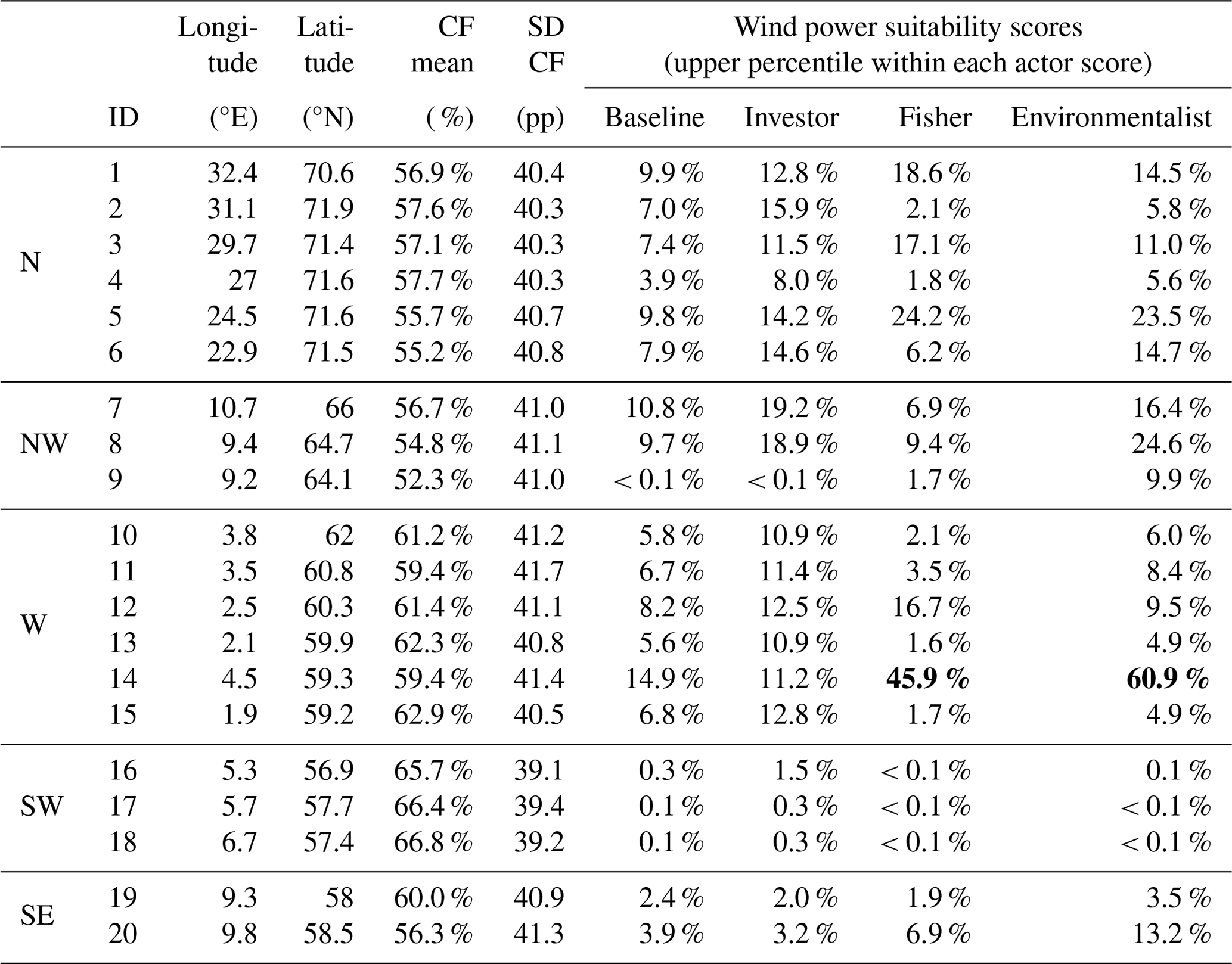
In Table 2, we have presented the coordinates of the selected candidate locations with the mean and standard deviation of the capacity factor based on the NORA3-WP grid cell. The suitability scores are calculated on the same grid as NORA3-WP, so the coordinates are exact (although rounded off). We have also included the wind power suitability scores as what upper percentile the location has within each actor score. Some of the scores of location 14 (UN) are highlighted as they violate the top 25 % score assumption for the fisher and environmentalist scores. The mean capacity factor ranges from 52.3 % to 66.8 %, while the standard deviations range from 39.1 to 41.7 pp. These locations thus have a wider range of mean capacity factors and a narrower standard deviation range compared to the NVE regions. S&S location 18 has the highest mean capacity factor of 66.8 % and the second lowest standard deviation of 39.2 pp, making it probably the best location among all the candidates. It resides within the NVE region Sønnavind A, which also has the highest mean capacity factor of the NVE regions (Table 1).

We divide the two candidate location sets into five regional groups, corresponding to the Norwegian naming of the NVE regions: north (N), northwest (NW), west (W), southwest (SW) and southeast (SE). Which locations belong to which group can be seen from the first columns of Tables 1–2. The northern groups are similar across the NVE and S&S, but the NVE regions are more spread out, while the S&S is closer to shore (except S&S 2). We have the same number of locations and roughly the same geographical spread in the northwest. The largest difference is that the S&S locations are much closer to shore, especially S&S 9. The opposite is true for the west coast, where S&S 12–13 and 15 are further out at sea than the NVE regions. The other S&S locations overlap with NVE regions for this group. The most striking aspect in the southwest group is that there are twice as many NVE regions as there are S&S regions. The NVE regions are also farther to the south and west. S&S 18 lies inside Sønnavind A, but we count S&S 18 as southwest, while Sønnavind A is the only NVE member in the southeast. Farther east, we also find S&S 19–20 in this group, closer to the Danish–Swedish–Norwegian border intersection in the Skagerrak. The two candidate sets both have some similarities and some interesting distinctions. This grouping is applicable when interpreting the correlation structure of the two location sets (see Sect. 3.2).

The NVE regions have a finite area, which we use for setting constraints on the maximum number of turbines. The S&S areas do not have this. To ensure a fair comparison, we do not allow S&S locations with more than 500 turbines. The median maximum number of turbines for the NVE regions is 486, so we have rounded this off to 500. This constraint corresponds to an area of 2143 km² using the same assumptions of 100 % utilization and 3.5 MW km⁻², comparable in size to Sørvest B or Nordavind B.

Now that we have our two sets of candidate locations, the NVE and S&S locations, we present a methodology for allocating turbines to the different wind farm locations.

3 Modern portfolio theory

There are some fundamental differences between a wind farm portfolio and a portfolio of financial assets:

1. One cannot borrow turbines (which corresponds to shorting assets in finance), meaning the portfolio weights have to be non-negative.

2. Selling or re-balancing the portfolio as time passes is not feasible. One can, in practice, only build more wind parks by investing more.

3. In financial investment theory, a higher risk should give a higher potential return, which is not necessarily valid for wind power production.

4. There is no equivalent to a risk-free interest rate for a portfolio of wind farms.

We argue, however, that the well-known diversification effect that we get when spreading financial investments across a large portfolio of assets is highly relevant when selecting sites for wind power production as well. In finance, we look for assets that have low, or even negative, correlation to lessen the impact of negative movements in the markets on the overall portfolio. If the value of one investment goes down, this will not be systematically associated with failure in other investments simultaneously. The corresponding phenomenon for wind farms is if wind conditions at one wind farm location are systematically associated with conditions at other locations. As one increases the distance between wind farms up to a point, the systematic association decreases, and the diversification effect increases (Solbrekke et al., 2020; St.Martin et al., 2015).

The classical approach for allocating wind farms seen in previous studies is modern, or mean variance, portfolio theory (Markowitz, 1952). The goal is, for a given target capacity factor, T_𝙘𝙛, to compose the portfolio that exhibits the minimum variance. Let $X_{ti}\in [\mathrm{0},\mathrm{1}]$ denote the stochastic variable for capacity factor from location i at time t and ${\mathit{X}}_t=(X_{t\mathrm{1}},\mathrm{\dots },X_{tm}{)}^{\prime }$, where m is the number of locations, $t=\mathrm{1},\mathrm{\dots },n$ and ^′ is the transpose operator. Let $\mathit{\mu }=({\mathit{\mu }}_{\mathrm{1}},\mathrm{\dots },{\mathit{\mu }}_m{)}^{\prime }=\mathbb{E}{\mathit{X}}_t^{\prime }$ denote the time-invariant expected value vector. Further, let Σ=Cov(X_t) denote the covariance matrix. Let $\mathit{w}=(w_{\mathrm{1}},\mathrm{\dots },w_m{)}^{\prime }$ denote the vector of non-negative portfolio weights, i.e., the proportion of the total number of wind turbines installed at each location. These must be non-negative because you cannot build a negative number of wind turbines. The portfolio capacity factor at time t, Y_t, can then be expressed as $Y_t={\sum }_{i=\mathrm{1}}^m{w}_i{X}_{ti}={\mathit{w}}^{\prime }{\mathit{X}}_t.$ The expected (time-invariant) capacity factor and the corresponding variance of the wind farm portfolio are, respectively, given by $\mathbb{E}{Y}_t={\sum }_{i=\mathrm{1}}^m{w}_i{\mathit{\mu }}_i={\mathit{w}}^{\prime }\mathit{\mu }\text{and}\mathrm{Var}\left(Y_t\right)={\mathit{w}}^{\prime }\mathbf{\Sigma }\mathit{w}.$ We want to find a portfolio that minimizes the portfolio variance for a given level of expected capacity factor, T_𝙘𝙛. We require the weights, w, to sum to 1: ${\mathit{w}}^{\prime }\mathbf{1}=\mathrm{1}$, where $\mathbf{1}=(\mathrm{1},\mathrm{\dots },\mathrm{1}{)}^{\prime }$ is a vector of length m. Then, we can formulate the optimization problem as

$$\begin{array}{rl}\text{minimize}& {\mathit{w}}^{\prime }\mathbf{\Sigma }\mathit{w},\\ \text{subject to}& {\mathit{w}}^{\prime }\mathit{\mu }=T_{\mathsf{\text{cf}}},{\mathit{w}}^{\prime }\mathbf{1}=\mathrm{1},\text{and}{w}_i\ge \mathrm{0},i=\mathrm{1},\mathrm{\dots },m.\end{array}$$

This is the simplest case with the bare minimum of constraints and corresponds to what Markowitz (1952) also used.

The formulation above does not exclude solutions where, for instance, only one wind turbine is placed far out in the Barents Sea or some turbines at every location. Small, spread-out wind farms are not a realistic solution since one must invest a lot in the infrastructure associated with each farm. Therefore, we rather prefer to cluster together many turbines at a few locations, which can be achieved by adding a constraint on the maximum number of nonzero weights, i.e., locations with more than zero turbines, called a position limit constraint. Another relevant constraint is the so-called box constraint, meaning setting a lower and upper limit on each location's weights and thus restricting the number of turbines allowed at said location. The box constraint avoids wind farms that are too large or too small. We derive maximum constraints based on the limited areas of the NVE regions (Table 1) and use a maximum of 500 turbines per location for the S&S locations. Tejeda et al. (2018) also use a box constraint with a minimum of 0 MW and a maximum of 250 MW per grid cell (≈550 km²).

For the position limit constraint, let 1(w>0) denote the indicator function, which equals 1 if w>0 and 0 otherwise, and let h denote the maximum number of nonzero turbine locations. For the box constraint, let $w_i\in [\mathrm{\ell },u]$ for $i=\mathrm{1},\mathrm{\dots },m$, where $\mathrm{0}\le \mathrm{\ell }\le u\le \mathrm{1}$. We write $w_i\in [\mathrm{\ell },u]\cup \mathit{\left\{}\mathrm{0}\mathit{\right\}}$ to allow for zero weights if combined with a position limit constraint.

The problem then becomes

$$\begin{array}{ll}{\displaystyle }\text{minimize}& {\displaystyle }{\mathit{w}}^{\prime }\mathbf{\Sigma }\mathit{w},\text{(objective)}\\ {\displaystyle }\text{subject to}& {\displaystyle }{\mathit{w}}^{\prime }\mathit{\mu }=T_{\mathsf{\text{cf}}},\text{(expectation constraint)}\\ {\displaystyle }& {\displaystyle }{\mathit{w}}^{\prime }\mathbf{1}=\mathrm{1},\text{(sum-to-one constraint)}\\ {\displaystyle }& {\displaystyle }{w}_i\in [\mathrm{\ell },u]\cup \mathit{\left\{}\mathrm{0}\mathit{\right\}},i=\mathrm{1},\mathrm{\dots },m,\text{(box constraint)}\\ {\displaystyle }& {\displaystyle }\text{and}\sum _{i=\mathrm{1}}^m\mathrm{1}(w_i>\mathrm{0})\le h\text{(position limit constraint)}.\end{array}$$

We consider five different scenarios with different combinations of constraints below. The most optimal solution would be the one with the fewest constraints, but it may be unrealistic due to the reasons listed earlier in this section.

We estimate the expected value vector μ and the covariance matrix Σ by the empirical mean and covariance of the hourly observations, i.e., $\widehat{\mathit{\mu }}=n^{-\mathrm{1}}{\sum }_{t=\mathrm{1}}^n{\mathit{X}}_t,\widehat{\mathbf{\Sigma }}=n^{-\mathrm{1}}{\sum }_{t=\mathrm{1}}^n({\mathit{X}}_t-\widehat{\mathit{\mu }})({\mathit{X}}_t-\widehat{\mathit{\mu }}{)}^{\prime }.$

The target capacity factor, T_𝙘𝙛, should be within the range of $\widehat{\mathit{\mu }}$. Otherwise, a solution will not exist. If $T_{\mathsf{\text{cf}}}={max}_i{\widehat{\mathit{\mu }}}_i$, all turbines must be placed on the location with the highest mean capacity factor.

We implement the position limit constraint by optimizing all combinations of h locations separately and selecting the minimum variance portfolio. We compare this approach to a stepwise approach by adding the location that improves the portfolio performance the most in each step, referred to as a sequential build-out. In the sequential build-out, we start building on the two locations the Norwegian Government already decided on (1500 MW at each) and then consider adding one other location (looping over all the other candidates) or building more turbines at the existing locations. We use the lower box constraint to keep the already-built turbines in the next iteration.

The number of turbines at a location is an integer number. In the portfolio optimization, we estimate weights as the proportion of 2000 turbines (30 GW). We get the number of turbines at a location by multiplying 2000 turbines with their portfolio weight and rounding off to the nearest integer. Even though the sum of the weights is 1, this rounding off may lead the total number of turbines to not equate 2000. We compensate for this by removing one turbine from the necessary number of locations in the estimated portfolios with too many turbines until the total is 2000 and correspondingly adding one turbine to the necessary number of locations with too few. The identified locations where this adjustment is applied are those with the number of turbines closest to being rounded down or up, respectively.

We use the R package quadprog (Turlach et al., 2019), which contains functions for solving quadratic programming problems, to optimize the portfolios under different constraint scenarios. For reproducibility purposes, the R code is made available at https://github.com/holleland/OffshoreWindPortfolios (last access: 20 January 2025; see data availability statement for further details).

3.1 Choice of temporal scale

The decision-maker’s choice of the temporal scale at which the portfolio variance is minimized is essential. We have chosen to use an hourly timescale, which is the highest temporal resolution in NORA3-WP and the most relevant scale for balancing the electricity grid. Aggregating to a coarser temporal resolution and finding the optimal portfolios corresponds to a higher focus on minimizing seasonal variation in the portfolio throughout the year. In what follows, we focus exclusively on using the hourly capacity factor in our analysis. We have also included a sensitivity analysis for some of our results to this choice of scale in Appendix A, including the effect various timescales have on the correlation structure (see Fig. A1).

3.2 Correlation structure

From the NORA3-WP data set, we estimate a mean vector $\widehat{\mathit{\mu }}$ and an empirical covariance matrix $\widehat{\mathbf{\Sigma }}$ for the NVE regions and the corresponding S&S locations. The covariance structure is important for the diversification effect. To simplify, say we have a portfolio of two assets, X and Y, such that the portfolio value is $wX+(\mathrm{1}-w)Y$, with weight $w\in (\mathrm{0},\mathrm{1})$. The portfolio variance is then

$$\begin{array}{}\text{(1)}& w^{\mathrm{2}}{\mathit{\sigma }}_X^{\mathrm{2}}+(\mathrm{1}-w{)}^{\mathrm{2}}{\mathit{\sigma }}_Y^{\mathrm{2}}+\mathrm{2}w(\mathrm{1}-w)\mathit{\rho }{\mathit{\sigma }}_x{\mathit{\sigma }}_y,\end{array}$$

where $\mathit{\rho }\in [-\mathrm{1},\mathrm{1}]$ is the correlation between X and Y, and σ_X and σ_Y are the standard deviations of X and Y, respectively. With all else fixed, reducing the correlation ρ will thus reduce the portfolio variance. Having wind power locations with a low correlation with other locations (perhaps even negative) is important for achieving diversification effects and a lower portfolio standard deviation.

We have presented the correlation matrices for the NVE and S&S locations as correlation heat maps in Fig. 2. Since the standard deviations are all in the same range (around 40 pp; see Tables 1 and 2), we use correlations instead of covariances as the scale is easy to interpret. The dashed red lines split the correlation matrices into blocks corresponding to the five location groups N, NW, W, SW and SE, described above. We have a substantial block structure following this grouping in the matrices, where the correlations are high within each block but low between them. The locations farthest to the north (Nordavind A–D, S&S 1–6) are almost uncorrelated with the remaining locations. The clear block off the northwest coast (Nordvest A–C and S&S7–9) also stands out as having a low correlation with the other blocks.

Figure 2 Correlation matrices for the hourly capacity factor at the 20 NVE regions and S&S locations. The dashed red lines split the locations according to the grouping of Tables 1–2.

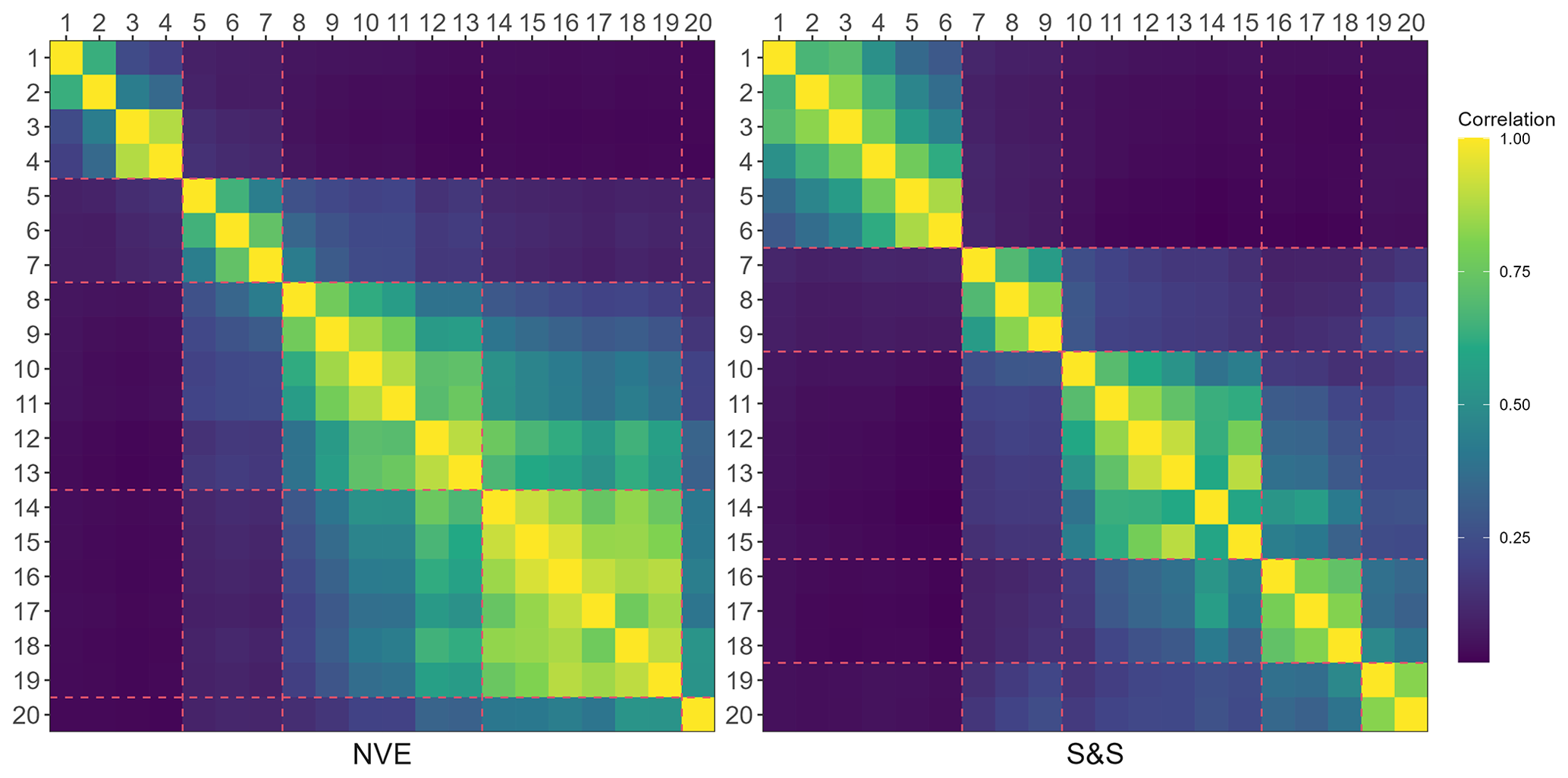
Further south, more locations are more closely packed, leading to a higher correlation between the blocks. The between-blocks correlations might be slightly higher for the southern NVE regions than the S&S locations, but these regions are also more evenly spread. In contrast, the S&S locations are more clustered in three more distinct groups (see map in Fig. 1d). For the NVE regions, Sønnavind A stands out as a location with low correlation with others and similarly for the two S&S locations in the Skagerrak (S&S 19–20).

3.3 Portfolio cases

We set up five sets of constraints under which we find the optimal portfolio. For scenarios below, with exactly five locations, our greedy algorithm for the position limit constraint loops over all combinations of five locations. For cases B and C, there are $\left(\genfrac{}{}{0ex}{}{\mathrm{18}}{\mathrm{3}}\right)=\mathrm{816}$ and $\left(\genfrac{}{}{0ex}{}{\mathrm{20}}{\mathrm{5}}\right)=\mathrm{15}\mathrm{504}$ such combinations, respectively, using the binomial coefficient notation. The cases are as follows:

• Case A has no constraints on the number of locations (benchmark portfolio).

• Case B has exactly five locations, where Sørlige Nordsjø 2 (SN2) and Utsira Nord (UN) are included.

• Case C has exactly five locations, not necessarily including SN2 and UN.

• Case D built 1500 MW at SN2 and 1500 MW at UN. Where to build 1500 MW next? (“as we go”/sequential build-out) until reaching 30 GW total. At each step, we either build where we already have farms or add one more location.

• Case E only builds on the first five sequentially selected locations from case D.

The resulting portfolios will depend on the value used for the target capacity factor, T_𝙘𝙛. For comparison purposes, T_𝙘𝙛 should be within the range of values for both the NVE regions and S&S locations. We therefore run the portfolio optimization for three values of T_𝙘𝙛: 58 %, 60 % and 62 %. For case A, we also solve the problem with a high resolution of T_𝙘𝙛 between 56 % and 65 %. These are high capacity factors compared to onshore wind farm portfolios. For example, Tejeda et al. (2018) use a 23 % capacity factor for their mainly onshore setting.

Case A will not necessarily give a realistic portfolio of wind farms as it has no restrictions on the number of locations. The optimal solution may involve many locations, some very small. However, it should give the portfolio with the lowest standard deviation, and, as such, it is a meaningful benchmark for the other portfolios. For cases B, C and E, we are restricted to only building on five locations, which will not result in very small wind farms. An interesting comparison is between case B and E as both require building on SN2 and UN and three other locations. They may result in the exact same portfolios. For the NVE regions, we do not allow for more turbines than the maximum number of turbines given in Table 1 and, correspondingly, no more than 500 turbines for S&S locations. Note that, for case E, we initially build five wind farms as in case D, corresponding to 7.5 GW installed capacity, and then distribute the remaining 22.5 GW in these five locations.

The sequential build-out in cases D and E starts with a portfolio of 1500 MW (100 turbines) at NVE regions Sørvest F and Vestavind F and, correspondingly, S&S locations 16 and 14. These are the locations where the Norwegian Government has decided to start building the first offshore wind farms, i.e., SN2 and UN. The initial portfolio of 1500 MW at each location will not fulfill the T_𝙘𝙛 requirement, as the capacity factor will be 62.6 %. We then, for all combinations of the existing wind farms and one new candidate location, find the optimal portfolios, using a box constraint to ensure that at least 1500 MW is kept on SN2 and UN. We also consider not adding new locations but merely building more on existing ones. Having found the optimal portfolios for each candidate location, we choose the one that minimizes the portfolio standard deviation and fulfills the target capacity factor constraint. We then update the box constraint with the weights of the best portfolio, and we start a new iteration, considering adding another location or building more on the existing ones in the same manner. In each iteration, we build 1500 MW (100 turbines) and repeat the process until 30 GW installed capacity or 2000 turbines have been placed. All the portfolios following the initial one must fulfill the T_𝙘𝙛 requirement. Since SN2 and UN have such a high mean capacity factor, we do not run cases D and E for T_𝙘𝙛=58 %. Having initially installed 1500 MW at SN2 and UN and then deciding where to place the next 1500 MW to achieve 58 % capacity factor, the only choice would be to place all 1500 MW at a location with a capacity factor of around 49 %. The minimum capacity factor for the NVE and S&S locations, respectively, is 54.6 % and 52.3 %. Hence, there exists no solution for the first iteration of the sequential algorithm when the target capacity factor is 58 %.

3.4 Underlying assumptions

For the analysis that follows, we make some simplifying assumptions that we want to make explicit. We refrain from imposing the current limitations on the Norwegian transmission grid to the optimization problem presented in this paper because they will likely change over the decades to come. Instead, we assume a “copper-plate Norway”, where the power grid is fully connected so that power production in the Barents Sea can have beneficial diversifying effects on the total power production in the event of no wind in the North Sea, for instance. Some offshore wind farms may not even produce energy for the Norwegian energy system but exclusively export energy to other European countries. The copper-plate assumption simplifies the problem but is not essential to the methodological approach that we propose. One alternative could be to assume no or a very limited transmission between the north and the south of Norway, which is more realistic today. This would then split the problem into two separate parts, on which we can apply the same analytical strategy separately, where the government distributes the total amount of installed power, 30 GW, say, between the two regions.

We do not explicitly take into account any energy system losses, such as electrical resistance losses, converter losses, maintenance losses, wake losses and auxiliary power consumption. Electrical resistance losses depend on the length of the cable. For the S&S locations, distance to shore is penalized in calculating the wind power suitability score. Hence, this is part of the decision of candidate selection. It is, however, not part of the placement of turbines. Wake losses are also important and would affect the total production from a wind farm, especially the larger ones (Barthelmie et al., 2009; Ghaisas et al., 2017). Quantifying wake losses would involve making assumptions about how the turbines are placed within a wind farm, but we focus on a more macro level. Our analysis, however, concerns the distribution of turbines across wind farms. Technology and innovation advancements in wind turbine and installation strategies may also reduce the effect of wake losses as we approach 2030 and beyond.

The wind power generated from the offshore fleet will enter an existing power market and become a portion of the higher-level electric power portfolio. One could imagine optimizing the allocation of wind power for this portfolio considering the current power sources. Hydroelectric power is the dominating energy source for producing electricity in Norway today (88.2 % in 2022; Statistics Norway, 2023). While hydropower can usually be controlled by opening or closing the flow of water, wind power is a non-dispatchable energy source. It must be utilized instantly unless stored (e.g., charging batteries, producing hydrogen or pumped-storage hydroelectricity). Therefore, it is appropriate that Norwegian hydropower will adapt to wind power rather than vice versa. Although combining wind and hydroelectric power is an interesting case study, we focus exclusively on the wind power portfolio.

Investment and maintenance costs will be primary drivers of offshore spatial planning. Costs will undoubtedly vary across different sites. For the S&S locations, factors that affect costs are implicitly regarded through the suitability score of each region. The suitability scores consider cost-increasing factors such as ocean depth and distance to shore, which are especially important for the investor actor's suitability score (Solbrekke and Sorteberg, 2023). After selecting the candidate locations, we only optimize the portfolios based on wind power resources and do not consider costs. A key parameter for a cost–benefit analysis is the price of electricity, which is difficult to forecast far into the future. Historical prices are irrelevant since 30 GW of wind power will nearly double the Norwegian electricity production (not considering changes in supply from other sources). A further analysis considering prices and costs may be a way to take this further, but it is outside the scope of this paper.

4 Results

In Fig. 3 we have plotted the optimal portfolios, with portfolio standard deviation on the x axis and portfolio capacity factor on the y axis, where the color distinguishes the two sets of locations we consider. In addition to the cases, we have included single-location portfolios as colored dots, i.e., portfolios with all turbines placed at one location, even if this violates the size constraints. These dots are simply the hourly mean and standard deviation of the capacity factor at each location. The curves are for case A with values of the capacity factor target between 56 % and 65 %. Since case A has the mildest restrictions, the curves represent the minimum standard deviation possible for this range of target values. These curves are called the efficient frontiers in modern portfolio theory. We note that the size of the diversification effect is large. Distributing wind turbines across multiple sites cuts the portfolio standard deviation nearly in two, from approximately 40 % to approximately 20 %, compared with collecting all turbines in a single location. The minimum standard deviation portfolios based on the NVE and S&S have standard deviations of 20.5 pp and expected capacity factors of 59.5 % and 58.9 %, respectively. Vestavind F has a mean capacity factor of 59.8 %, which is quite close to 59.5 % of the NVE minimum standard deviation portfolio and a corresponding standard deviation of 41.3 pp. Compared to the 36 % reduction found by Drake and Hubacek (2007), we find a potential geographical diversification effect of 50.4 % from placing all power at Vestavind F to the minimum standard deviation portfolio of the NVE locations at T_𝙘𝙛=59.8 %, indicated by the blue arrow in Fig. 3.

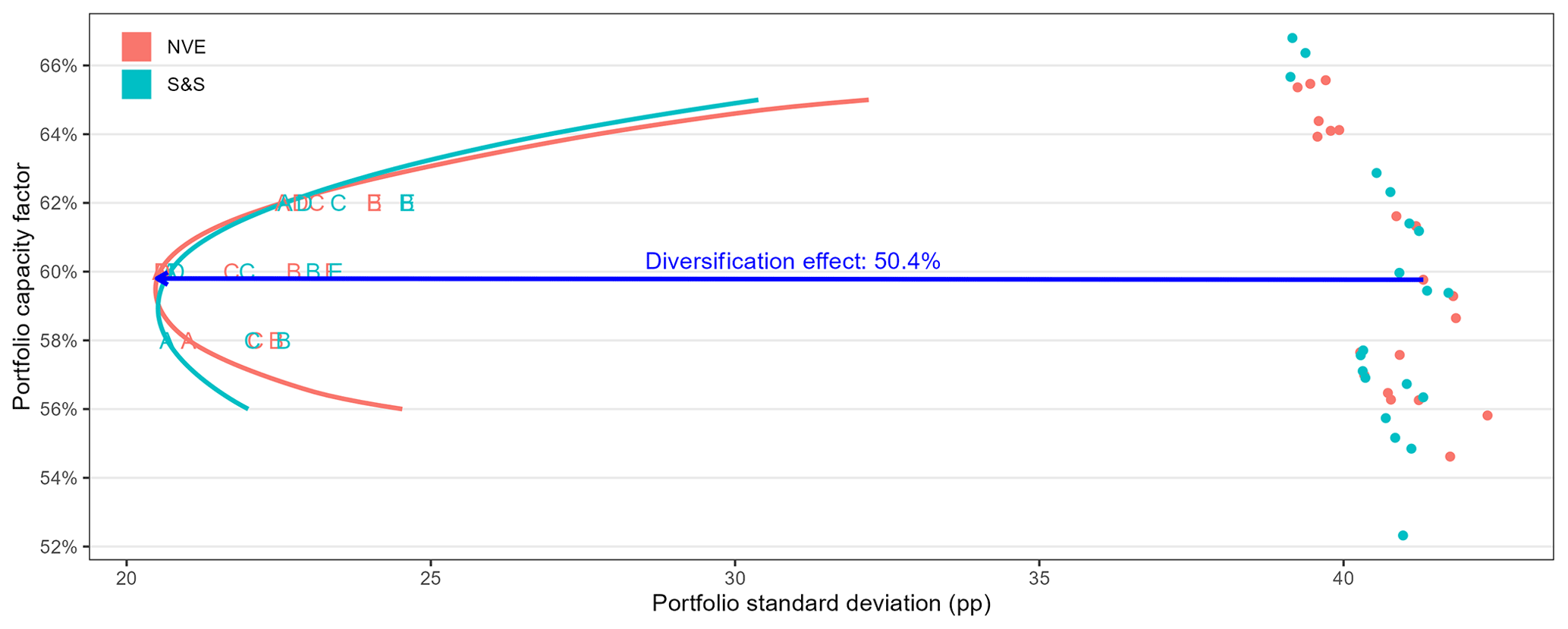
Figure 3 Portfolios summarized by portfolio capacity factor and standard deviation in percentage points (pp) for the NVE and S&S locations. The dots are one-location portfolios, while the letters represent the different-case portfolios for capacity factor targets 58 %, 60 % and 62 %. The curved lines are efficient frontiers for case A, i.e., optimal portfolios for a finer sequence of capacity factors from 56 % to 65 %. The blue arrow indicates a 50.4 % reduction in portfolio standard deviation from placing all turbines at Vestavind F to the minimum standard deviation portfolio of the NVE locations for case A with T_𝙘𝙛=59.8 %.

For financial investments, intuition says a higher risk should give a higher potential return. In our case of wind power production, however, we see that the highest-power-producing locations also have the lowest standard deviations. The efficient frontier curves in Fig. 3 illustrate this point on a portfolio level. As the target capacity factor decreases, the standard deviation decreases to a point (around T_𝙘𝙛= 59 %), where it turns. Decreasing the target capacity factors beyond this point will increase the portfolio standard deviation. Therefore, the portfolios for case A at 58 % have a higher standard deviation than the corresponding at 60 % and should never be chosen. The same effect is present in case C, going from 58 % to 60 %. The diversification effect on the portfolio standard deviation is strong, so the best portfolios must include some relatively high- and low-producing locations. However, to achieve a 58 % capacity factor, the portfolio must consist of more low-mean locations with a higher standard deviation. The reason for this U-turn is the lack of a risk-free asset among the candidate locations. There is no equivalent to placing capital in the bank, so to speak, at a risk-free interest rate in wind power production, which is necessary for a monotonically increasing efficient frontier.

Case A has fewer constraints than any other scenario and should give the portfolio with the lowest standard deviation for the same capacity factor target. We can see from Table 3, presenting summary statistics for the different portfolio cases, and Fig. 3 that this is the case. Without any constraints on the number of locations, case A tends to have many wind farms, ranging from 11 to 17 across all capacity factor targets and location sets. Table B1 shows the actual number of turbines per wind farm location, and the turbines for case A are spread out all over NEZ, although less so for the 62 % target capacity factor cases. It is relevant to compare case A to the sequential build-out case D, as both have no restrictions on the number of wind farms. The number of wind farms for these cases is similar. However, we have small wind farms ranging from 4 to 63 turbines. Restricting the optimization problem to five locations (cases B, C and E) seems to avoid this issue because they result in the minimum number of 158 turbines at one location. We impose restrictions on the maximum number of turbines for the different locations. The largest NVE farm is 527, while, for S&S cases, the 500-turbine upper limit is met in 6 of the 13 scenarios.

Table 3 Summary of the different wind farm portfolios for the two sets of potential locations, cases, expected capacity factor (CF) and the standard deviation (SD) of the portfolio given in percentage points (pp). The number of wind farms (No. WF) with turbines and the smallest (Min turb.) and largest (Max turb.) wind farm. The CF 5 % and 95 % columns are the 5th and 95th percentiles of the portfolio capacity factor, respectively.

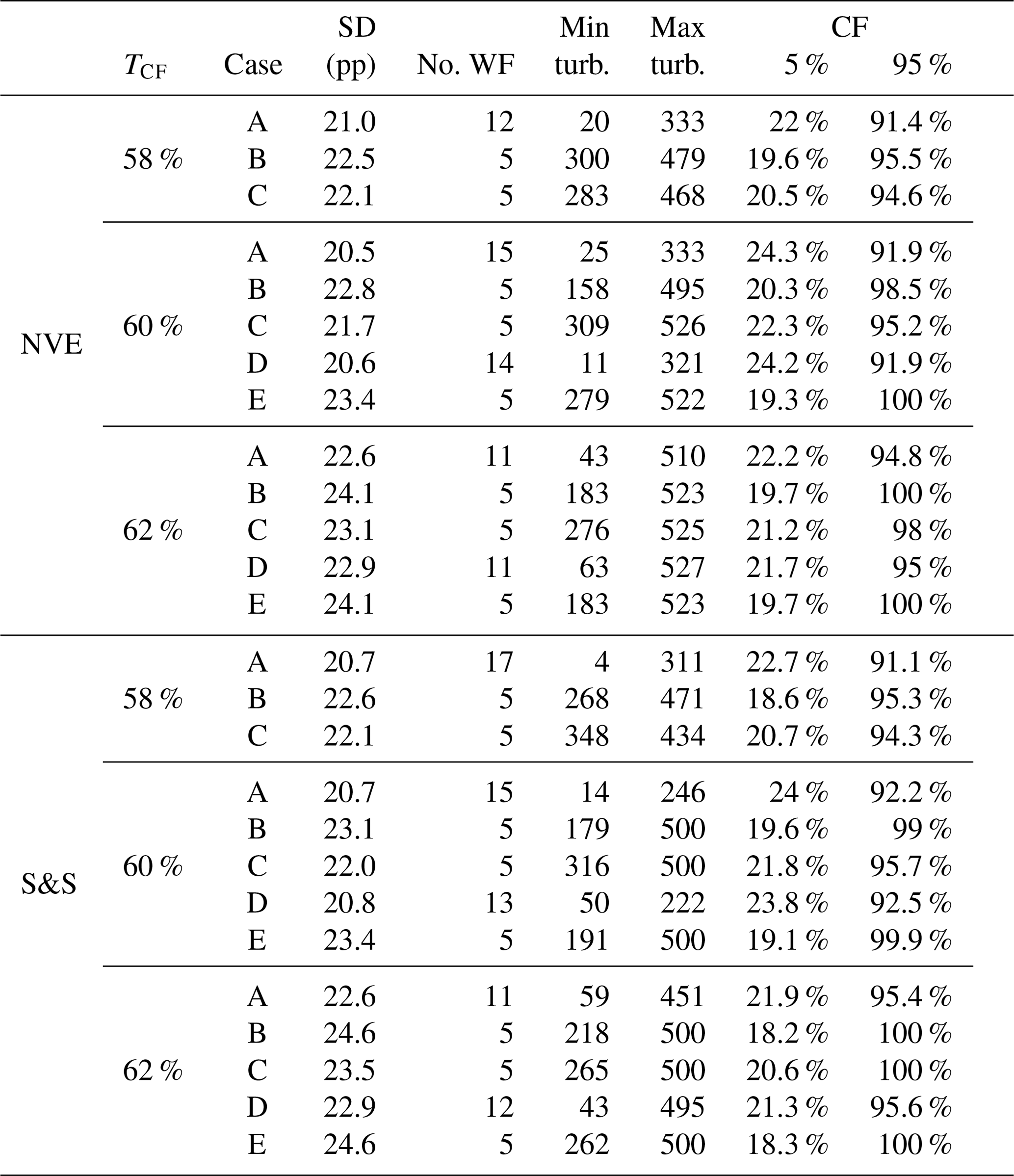
For cases B, C and E, we build five wind farms, and in cases B and E, UN and SN2 are required to be included. In terms of standard deviation, the ascending order of these cases should always be C–B–E. This is because case C has the fewest requirements. It does not need to include UN or SN2. Case B has to include UN and SN2, but we can build as few turbines as we want there. For case E, we must have at least 1500 MW (100 turbines) installed capacity on both UN and SN2, as this is the initial portfolio. From Table 3 and Fig. 3, we see that the ascending order holds, but for capacity factor 62 %, cases B and E have the same standard deviation up to the accuracy of the table. Looking at the exact distribution of the 2000 turbines, presented in Appendix Table B1, we see that the portfolios are exactly the same for the NVE locations but with minor differences for the S&S locations.

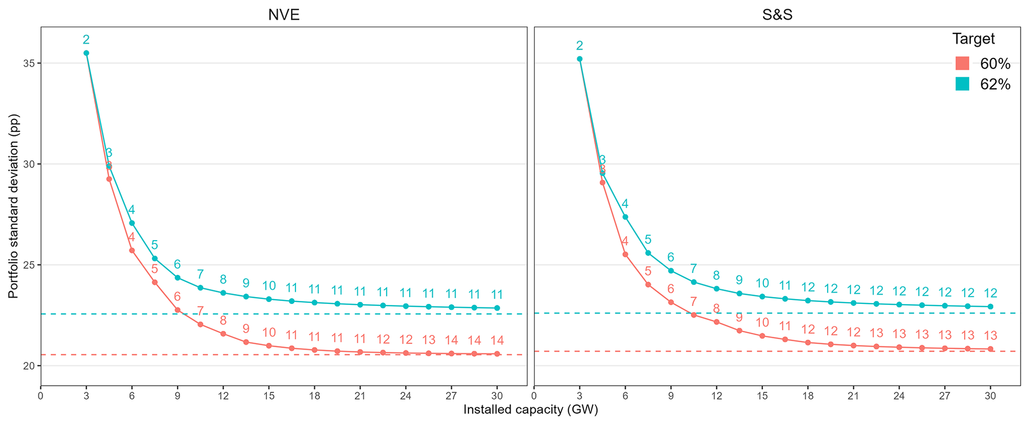
Figure 4 Standard deviation (pp) as a function of installed capacity (GW) for sequential build-out in case D, colored by target capacity factor and panels by candidate location set. The numbers give the number of wind farms at each iteration. The dashed lines are the standard deviations for the corresponding portfolios for case A.

For the sequential build-out in case D, we have plotted the decreasing portfolio standard deviation as a function of the sequentially increasing installed capacity in Fig. 4. We have included the standard deviation of case A for the respective setups as dashed horizontal lines, representing the lower threshold of what is possible to achieve. The numbers correspond to the number of wind farms included in the portfolio at the given iteration. The diversification effect is apparent. As expected, the portfolio standard deviation decreases rapidly as the number of locations increases, converging towards an asymptote. Building around 5–7 wind farms achieves a high diversifying effect on the standard deviation. In fact, with only three locations for the NVE case with a target capacity factor of 60 %, the reduction in standard deviation compared to placing all turbines at Vestavind F is roughly the same as what Drake and Hubacek (2007) found (37.8 %). This estimate is conservative as the target capacity factor is lower at Vestavind F compared to the 60 % target. A supplementary animation for case D at 60 % target capacity factor for the NVE regions, showing the turbine distribution on a map for each iteration, is available on the GitHub repository associated with the article (see the data availability statement). Remember that the initial portfolios with only two locations (UN and SN2) are not optimized; i.e., the weights are not estimated but fixed to 0.5 and 0.5. Therefore, the initial portfolio does not fulfill the target capacity factor constraint. For the 62 % cases, we see that after having installed 16.5 GW at 11 locations and 18 GW at 12 locations, we do not include new NVE and S&S locations, respectively. It is better to extend the existing ones. At 60 %, the corresponding numbers are 27 GW at 14 and 22.5 GW at 13 locations. We can also see from Fig. 4 that the portfolio standard deviation approaches the value of case A with a negligible difference, and for 60 % NVE, it reaches it exactly. Note that case E does not have the same standard deviation as the five wind farms in Fig. 4, because at that point in the build-out, UN and SN2 have a minimum of 20 % of the installed turbines each, while, for case E at 30 GW, they are only required to have 5 %.

We see in Fig. 3 that the diversification effect of 50.4 % would have been nearly the same if we compared it against the S&S efficient frontier for case A. Having the same number of locations and similar box constraints for the wind farm locations, we can also compare the portfolios between the two sets of locations. From Fig. 3 and Table 3, the NVE portfolios outperform the S&S portfolios case by case in terms of variance for the most relevant capacity factors 60 % and 62 %, but the differences are slight. The minimum standard deviation on the efficient frontiers is the same, but the NVE has a higher capacity factor at that point on the curve. For capacity factors below this minimum standard deviation portfolio, the S&S locations have lower standard deviations for case A and almost the same for cases B–C. The only notable case in terms of robustness is case B as it has a lower standard deviation at 58 % than at 60 %. Above 62 %, the efficient frontier of S&S lies above the NVE with a large difference at 65 %. This is because, at 65 %, we approach the maximum capacity factor of the NVE regions (65.6 %). At the same point, S&S still has three locations well above 65 % and thus has a higher potential for diversification.

We have included a sensitivity analysis in the choice of temporal scale for the NVE locations under case A at a target capacity factor of 60 %. The temporal scales considered are hourly, daily, weekly and monthly. The number of turbines per NVE candidate location has been aggregated to the five NVE regions (from northwest to southeast), resulting in Table A1. Aggregating to lower temporal scales increases the dependence between different sites, implying that we need a longer distance between wind farms to obtain diversification effects. Since we keep the candidate locations fixed, the turbines are spread over fewer locations at lower temporal scales. For more details, see Appendix A.

As the Norwegian Government has decided to start building wind farms at SN2 and then UN, they currently have a sequential build-out strategy. It is interesting to compare this to a global optimization scenario where the perspective is how the offshore wind power portfolio looks when all is said and done, i.e., when all the offshore areas for the 30 GW wind power are settled. We have already seen that the standard deviation of the sequential case D approaches that of A, but the distribution of the turbines is also essential. Comparing case A to case D in Table B1, they seem very similar in terms of where to build the wind farms. In most cases, where a different location is selected, it is a neighboring location.

We note that UN is not included in case A for portfolios with a capacity factor above 58 % (Table B1). At 62 %, cases A and D have selected the same locations except for UN (Vestavind F/S&S 14). Interestingly, in the iterations of the sequential build-out, we never build any turbines at UN except for the 100 we started with (Tables B2–B3 in the Appendix). In fact, in all the cases where UN is not required (cases A and C), we do not build any turbines there if T_𝙘𝙛>58 %, suggesting that UN is likely not a highly suitable location when only concerned with minimizing the standard deviation and under our other assumptions. On the other hand, SN2 is included in all S&S A cases and NVE cases except the 58 % capacity factor. From Table B1, we can also see that SN2 is included in all cases when T_𝙘𝙛=62 %.

For the other locations, Sønnavind A/S&S 18 and Vestavind A/S&S 10 stand out as locations selected in most cases. These location pairs are almost the same in both sets. Sønnavind A/S&S 18 has the highest capacity factor and among the lowest standard deviations, making it an attractive location. Vestavind A/S&S 10 is likely included due to its diversification effect. Among the S&S locations, S&S 10 is far from the central cluster off the west coast and the furthest away from UN for cases where this is mandatory. The latter also holds for the NVE region. Based on the correlation matrices and with a maximum of five wind farms, choosing one location from each of the five regional groups seemed natural to obtain the most considerable diversification effect. For cases B, C and E, such a clear pattern is not seen. We always place one or two wind farms in the northern and western groups. If two wind farms, they are always the ones that are farthest away from each other (Nordavind A and D, Vestavind A and F, S&S 1 and S&S 6, S&S 10 and S&S 14). In the south, Sørvest F/S&S 16, Sønnavind A/S&S 18 or both are included. There is a tendency to follow the correlation matrix blocks (see Fig. 2) for the 60 % case C, where we get two farms in the north, one in the northwest, one in the west and one in the south. At 62 %, for the same case, turbines are placed at the two farms in the south, probably to achieve the capacity factor requirement.

One interesting point is that for the 60 % capacity factor case D, the first selected location S&S 8 and Nordvest C, all and almost all of the 100 new turbines placed in that iteration are put at the new site (see Tables B2–B3), respectively. Choosing these locations and placing virtually all new turbines there pushes the capacity factor from 62.6 % to 60 %. We do not build any more turbines at S&S 8; for Nordvest C, only three turbines follow the initial 98. This observation indicates that these selected locations in the first iteration are suboptimal for minimizing the variance, as the procedure has to assign turbines to them to meet the expectation constraint. For comparison reasons, we keep the strict expectation constraint, but one could imagine a different approach (e.g., a gradual decrease from the initial 62.6 % capacity factor to the target).

5 Concluding remarks

We have shown how to adapt modern portfolio theory to the challenge of allocating offshore wind turbines across a range of suitable wind farm regions. The constrained optimization due to the limited area makes the resulting portfolios more sensible. Limiting the number of wind farms has not been done in a wind farm portfolio context, likely because most earlier studies have not focused on offshore wind. When not using a maximum number of wind farms, our results indicate that the Norwegian Government's apparent strategy of sequentially opening new offshore regions for wind power deployment may lead to a suboptimal final solution to the allocation problem, but it is seemingly very close or even equal to the global solution. However, a step-by-step build-out may, after all, be a good idea, as it likely provides better intermediate portfolios on the way towards 30 GW installed capacity.

The NEZ has considerable potential for obtaining a diversified offshore wind power portfolio. Among our candidate locations, we found a clear block structure in the wind power correlation matrices (Fig. 2). Spreading the wind farms across these blocks dramatically reduces the total variation. The maximum potential diversification effect we found was 50.4 % for a capacity factor of 59.8 %. From the sequential build-out case, we found that the diversification effect was also large after including only a few locations (5–7).

Deciding where to place wind farms and how to construct an investment portfolio are two different problems. We have highlighted some of these fundamental differences and how these can be taken into account or can be seen in the results of a modern portfolio analysis. The U-turning efficient frontier could also occur for financial investment portfolios, but in such applications, a risk-free interest rate is usually included in the pool of assets. A consequence of the U-turn is a unique minimum standard deviation portfolio that is not an extremity in the expected output variable.

The 20 areas that the Norwegian Water Resources and Energy Directorate (2023) has identified seem reasonable from our perspective. Using the wind power suitability scores of Solbrekke and Sorteberg (2023) to identify 19 locations and adding Utsira Nord resulted in a similar pool of candidate locations, with some distinctions. The performance of the resulting portfolios for the two candidate location sets was satisfactory. The NVE portfolios did slightly better for low-variance portfolios and S&S slightly better for high-capacity-factor portfolios in the case with the fewest restrictions. In any case, the differences are minor and indicate that our results are robust against the selection of candidate locations.

We do not expect the Norwegian Government to decide where to place each turbine in the NEZ solely based on this work. Given the points already discussed, this paper merely contributes to the discussion regarding the spatial planning of offshore wind farms in the NEZ. Getting reliable cost estimates for building and maintaining offshore wind farms at different locations should be part of such a decision. It could also be that the parameters we have optimized the portfolios under do not correspond with the risk aversion of the decision-makers. Accepting a more volatile wind farm portfolio with lower infrastructure investments seems like a reasonable compromise.

Appendix A: Sensitivity to temporal resolution

In this section, we have performed a sensitivity analysis of the choice of hourly temporal scale. One could argue that other timescales are more relevant, and the turbine distribution will depend on the choice of scale. We have aggregated the NORA3-WP hourly capacity factor data at the different NVE locations to daily, weekly and monthly averages and calculated the empirical covariance matrices on the various scales. The mean capacity factor per location ($\widehat{\mathit{\mu }}$) will not change due to this scaling. The corresponding correlation matrices are presented in Fig. A1. We then solve the turbine distribution problem using modern portfolio theory for NVE case A with target capacity factor of T_𝙘𝙛=60 % and sum the total number of turbines per NVE region. The number of turbines per region is presented in Table A1.

Clearly, the distribution of turbines depends on which timescale a decision-maker is interested in minimizing the variance. Aggregating from an hourly scale will increase the correlation of wind power production between sites (cf. Fig. A1) and require larger distances between wind farms to obtain diversification effects. This results in concentrating the 2000 turbines on fewer locations, which can be seen in the final column of Table A1. Hourly and daily will be qualitatively very similar, but the diversification potential is significantly reduced for the Norwegian offshore wind power portfolio at weekly and monthly scales.

Table A1 Number of turbines per NVE region from case A for the NVE locations at different temporal resolutions.

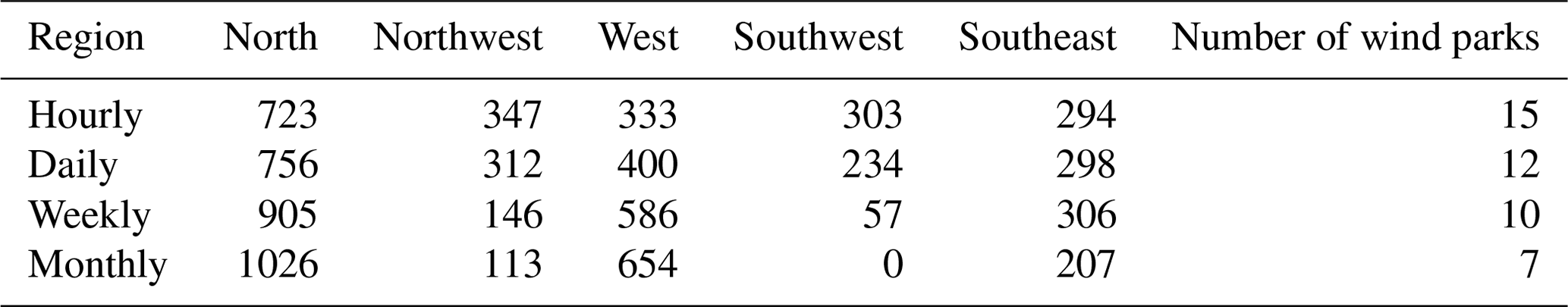
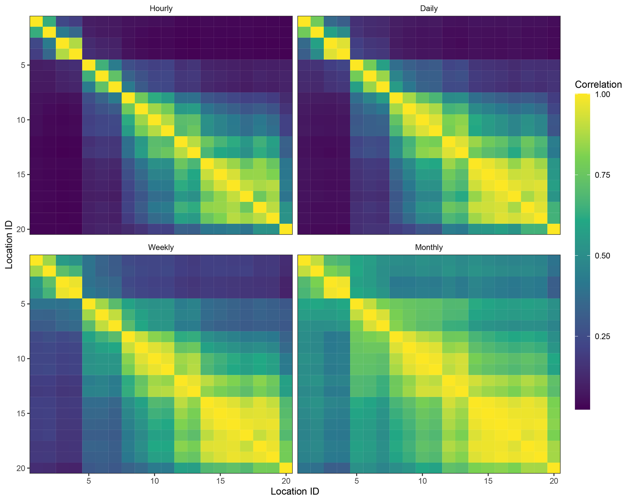
Figure A1 Correlation matrices for capacity factor for the NVE locations at different timescales: hourly, daily, weekly and monthly.

Appendix B: Additional tables

In this Appendix, we have included tables with further details about the allocation of turbines for the different cases and candidate locations.

Table B1 Number of turbines per location for the portfolio cases (A–E) and target capacities (58 %, 60 %, 62 %), with NVE locations at the top and S&S below. The far right column contains the maximum turbine constraints per location.

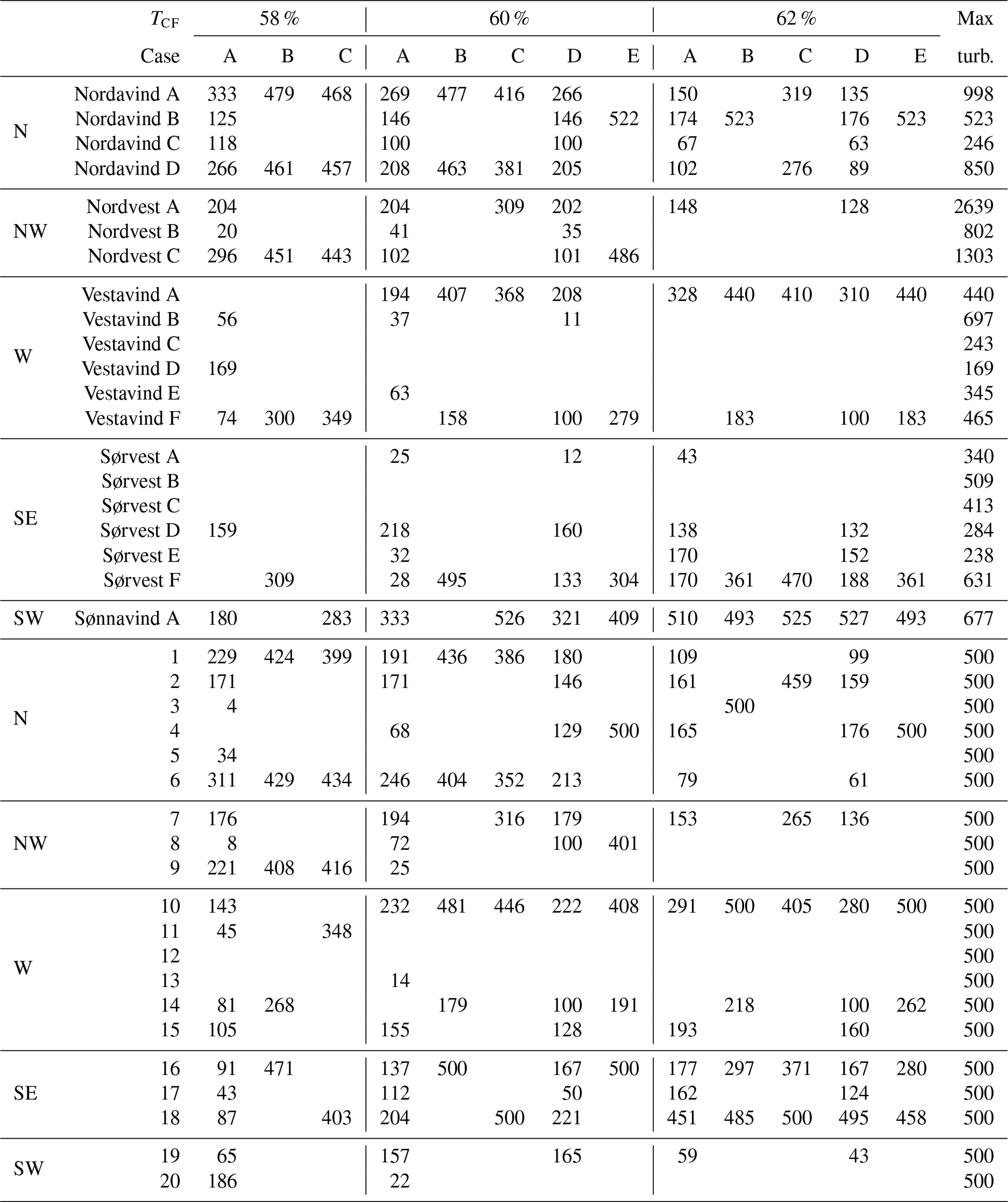
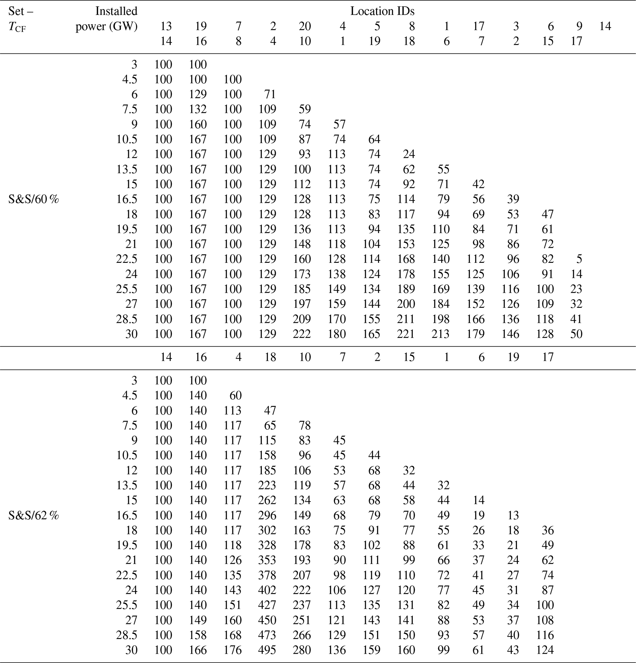
Table B2 Number of turbines for each iteration of the sequential build-out in case D for the different targets (60 %, 62 %) and candidate location set NVE.

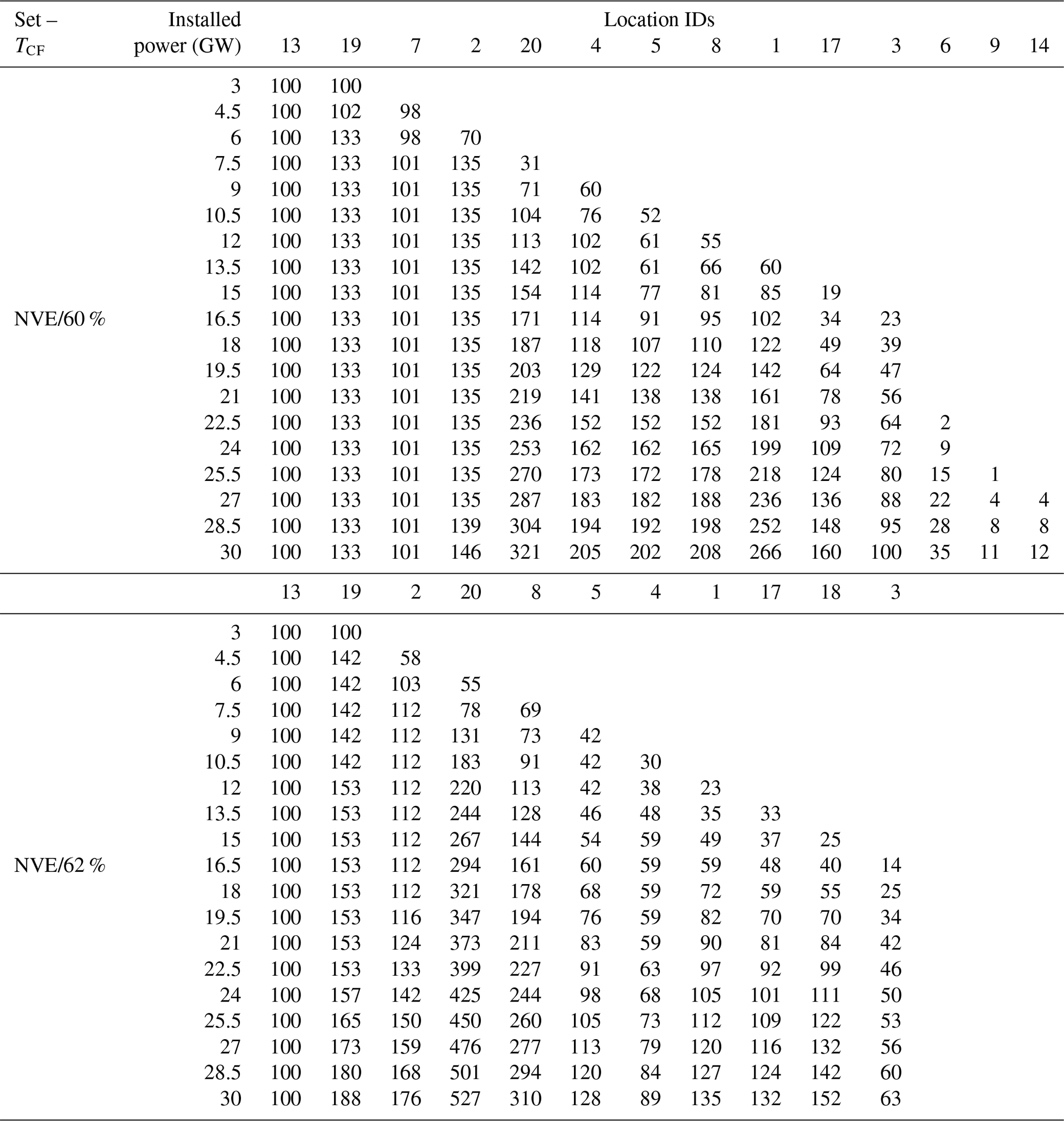
Table B3 Number of turbines for each iteration of the sequential build-out in case D for the different targets (60 %, 62 %) and candidate location set S&S.