the Creative Commons Attribution 4.0 License.
the Creative Commons Attribution 4.0 License.
 | 28 Apr 2025
Modular deep learning approach for wind farm power forecasting and wake loss prediction
Timothy Verstraeten
Pieter-Jan Daems
Ann Nowé
Jan Helsen
Power production of offshore wind farms depends on many parameters and is significantly affected by wake losses. Due to the variability in wind power and its rapidly increasing share in the total energy mix, accurate forecasting of the power production of a wind farm becomes increasingly important. This paper presents a novel data-driven methodology to construct a fast and accurate wind farm power model. The deep learning model is not limited to steady-state situations but captures the influence of temporal wind dynamics and the farm power controller on the power production of the wind farm. With a multi-component pipeline, multiple weather forecasts of meteorological forecast providers are incorporated to generate farm power forecasts over multiple time horizons. Furthermore, in conjunction with a data-driven turbine power model, the wind farm model can also be used to predict the wake power losses. The proposed methodology includes a quantification of the prediction uncertainty, which is important for trading and power control applications. A key advantage of the data-driven approach is the high prediction speed compared to physics-based methods, enabling its use in applications that require forecasting multiple scenarios in real time. It is shown that the accuracy of the proposed power prediction model is better than for some baseline machine learning models. The methodology is demonstrated for two large real-world offshore wind farms located within the Belgian–Dutch wind farm cluster in the North Sea.
- Article
(8040 KB) - Full-text XML
- BibTeX
- EndNote


Over the last decades, renewables have been expanding quickly, but the global energy crisis has kicked them into an new phase of even faster growth. Global wind capacity is expected to almost double in the upcoming 5 years, with offshore projects accounting for one-fifth of the growth (IEA, 2022).
Due to the rapidly increasing share of wind power in the total energy mix and its variable and intermittent nature, accurate forecasting of the power production of wind farms is becoming increasingly important for wind farm operators, balancing responsible parties (BRPs) and transmission system operators (TSOs). In addition, as wind turbines and wind farms are getting larger in scale, their influence on the wind flow and the resulting wake effects is becoming more pronounced.
The energy production of a wind farm is influenced by many factors (Lee and Fields, 2021). First of all, the energy production of an individual wind turbine depends on many parameters. The type of the turbine (with its specific mechanical and electrical design and control systems) and the wind speed are the most important parameters. Also wind turbulence and air density have an important influence on the power production. Furthermore, a turbine can be derated due to technical reasons or be limited in power by a wind farm power controller.
Secondly, the energy production of a wind farm can be significantly reduced by wake losses. Wind turbines modify the airflow for downstream turbines, resulting in velocity deficits and increased turbulence. Reduced velocity of the air results in power losses, whereas increased turbulence results in a faster recovery of the velocity deficit (Sanderse et al., 2011). The magnitude of wake losses depends mainly on the layout of the wind farm (distance between the turbines, orientation of turbine rows and length of the cross-section of the farm) and the wind direction (Barthelmie et al., 2009) but also on other parameters, such as the wind turbulence intensity, atmospheric stability and surface roughness. The power loss of a downstream turbine can reach 40 % in full-wake conditions (Barthelmie et al., 2009). When averaged over all different wind directions and wind speeds, annual power losses of a complete farm due to wake can range between 5 % and 20 %. Studies indicate that active wake control by applying yaw and/or induction control on the turbines may reduce wake losses and hence increase the power production of the farm (Boersma et al., 2017; Verstraeten et al., 2021). However, validation of the possible power gain under real-world conditions in a wind farm is still an active field of research (Bossanyi and Ruisi, 2021; Fleming et al., 2016, 2020).
Thirdly, the characteristics of the wind inflow into a wind farm (wind speed, wind direction, turbulence intensity, air density) are influenced by the environment surrounding the wind farm. Upstream wind farms may cause a reduction in the wind speed and an increase in the turbulence intensity (Porté-Agel et al., 2020; Pettas et al., 2021). Wind blockage by neighbouring farms and the wind farm itself may also reduce the inflow speed and deflect the inflow direction (Porté-Agel et al., 2020; Bleeg et al., 2018; Strickland et al., 2022). Also the proximity of coastlines can exert a significant influence on the wind characteristics, primarily attributable to differences in roughness and heat capacity between sea and land (Van Der Laan et al., 2017).
1.1 Wind and wake flow modelling
The modelling of wind and wake flows within wind farms is challenging and has been an active field of research for decades. In addition to affecting the power production, wake turbulence also impacts the loading of the turbines (Nejad et al., 2022). A wide range of different models have been developed. Based on the amount of detail they capture, they can be classified into three classes: low-fidelity, medium-fidelity and high-fidelity models. Each of these types of models have some advantages and drawbacks. Low-fidelity models describe only the dominant wake characteristics and are mostly limited to steady-state simulations and homogeneous 2D wind inflows. These models are usually relatively fast (on the order of seconds on a personal computer (PC) for a steady-state simulation) but need tuning of some hyper-parameters and have a lower accuracy (Jensen Park model, Jensen, 1983; FLOw Redirection and Induction in Steady State, FLORIS, NREL, 2025b; curled wake model, Martínez-Tossas et al., 2019, 2021; and TurbOPark, Nygaard et al., 2020). In recent years, some further developments have made it possible to also model some heterogeneous and dynamic environmental conditions (e.g. FLORIDyn, Gebraad and Van Wingerden, 2014; Becker et al., 2022; UFLORIS, Foloppe et al., 2022). On the other side of the spectrum, high-fidelity models, based on the 3D Navier–Stokes equations, describe flows in high detail. Large-eddy simulations (LESs) resolve these equations on a coarse mesh and approximate smaller-scale eddies with subgrid models (Sanderse et al., 2011). The main drawback of this type of model is the high computing load (on the order of days on a computing cluster). Some examples of high-fidelity simulators are SOWFA (NREL, 2025c), PALM (University of Hannover, 2021) and SP-Wind (Sood et al., 2022). Finally, medium-fidelity models (such as DWM, Larsen et al., 2007; FAST.Farm, NREL, 2025a; and WAKEFARM, Schepers, 1998) are based on simplifications of the Navier–Stokes equations. Despite the simplifications, the computing time for medium-fidelity models remains significant (on the order of minutes on a PC) (Boersma et al., 2017).
In contrast to physics-based models, data-driven techniques are not based on prior knowledge about the physical behaviour of the turbines or the airflow. Instead, they focus on fitting a general model with data. Recent developments related to deep learning resulted in a significant leap forward in the modelling of large and complex data sets (LeCun et al., 2015).
Wind farm operators usually have huge amounts of historical supervisory control and data acquisition (SCADA) data acquired by the instrumentation on their turbines. These data can be leveraged by machine learning techniques (Verstraeten et al., 2019). Taking advantage of this large amount of detailed information, accurate models of the wind farm and turbines can be built depending solely on this farm-specific data and not on any other, often less specific or less accurate, data sources such as theoretical turbine power curves and weather forecast data.
Commercial weather forecast service providers (e.g. StormGeo; Koninklijk Meteorologisch Instituut van België, KMI) nowadays provide weather forecasts for specific geographical locations. However, forecasts by distinct providers can differ between each other significantly, as they can be based on different weather models and data. In addition, although they provide forecasts for a specific geographical location such as the position of an offshore wind farm, they typically do not take into account the influence of the immediate surroundings of the wind farm, such as the presence of neighbouring offshore wind farms and the influence of coastlines. Moreover, they may not be able to provide all weather parameters that are required as inputs for an accurate wind farm power model, and the provided variables may be calibrated differently than the instrumentation data used during the training phase of the data-driven model.
1.2 Problem statement
The problem statement that this paper addresses is constructing a fast and accurate farm power forecasting model which captures the temporal dynamics of the wind inflow as well as the behaviour of the farm power controller. A deep learning nowcasting power model is trained solely with SCADA data from the wind farm itself. Therefore, this farm power model is unique and independent of any weather forecast data. In a multi-component pipeline, this single farm power model can be interfaced with multiple weather forecast services (from third-party providers) to forecast the wind farm power over multiple time horizons. The proposed model is capable of forecasting the farm power in a few milliseconds on PC, with an accuracy that surpasses the accuracy of other state-of-the-art data-driven models. This demonstrates that the proposed farm power forecasting model can be used for applications that require both simulation of the farm power controller and fast power forecasting, such as, for example, in a reinforcement control setting where fast evaluations of many possible controller actions are required.
1.3 State of the art of data-driven wind power forecasting
This work distinguishes itself from other publications about data-driven wind power forecasting in several aspects.
In the literature, many models can be found for the power prediction of an individual turbine (Perez-Sanjines et al., 2022; Zehtabiyan-Rezaie et al., 2023; Ti et al., 2021; Kisvari et al., 2021; Lin and Liu, 2020; Daenens et al., 2024) (whether or not they were superposed afterwards onto a farm). The model proposed in this paper predicts the power of a complete wind farm as a whole, without the need for a model for the individual turbines.
Whereas wind farm operators typically possess huge amounts of SCADA data, due to confidentiality reasons, such data are rarely accessible to the research community. Consequently, in many publications about wind farm power and wake modelling, simulation data are generated with physics-based models (low-fidelity static model Floris, Yin and Zhao, 2019; Park and Park, 2019; mid-fidelity models, Zehtabiyan-Rezaie et al., 2023; Ti et al., 2021), often only for relatively small virtual wind farms and for a limited set of wind conditions. In contrast, the data used in this paper are SCADA data from two large real-world offshore wind farms.
Many data-driven models in the literature have only a limited set of input features (e.g. restricted to wind speed, Perez-Sanjines et al., 2022; restricted to wind direction or historic wind power series, Wang et al., 2017), whereas the wind farm power model presented in this paper includes many more input parameters, all having a direct physical influence on the farm power (among others, air density, turbulence intensity, wind direction variance, wind farm power set point and power limitations due to technical reasons). It is shown that adding these additional input parameters significantly improves the accuracy of the model.
Data-driven wind farm power models found in the literature are often based on data with a relatively coarse time resolution (10 min or 1 h) (Liu et al., 2021; Kisvari et al., 2021; Wang et al., 2021). However, in this work, the wind farm power prediction model is trained with time series of 1 min SCADA data in order to be able to capture the temporal dynamics of the inflow wind and the effect of set point changes of the farm power controller (for which 1 min SCADA data were available for this work). In particular, the influence of inflow wind speed variations on the farm power production is analysed in this work.
A multi-horizon data-driven wind power forecasting method based on time series forecasting is proposed by Pombo et al. (2021). This method results only in good predictions for short-time-horizon forecasting. In order to obtain long-term multi-horizon forecasts, the multi-component pipeline proposed in this work incorporates weather forecast data for multiple time horizons as a separate component, without modification of the nowcasting farm power model trained solely with SCADA data from the wind farm. Another advantage of the multi-component pipeline is that the sensitivity to multiple physical input features can be analysed. This is not possible for a model that consists of one single black box. Sensitivity plots can be interpreted easily by wind energy professionals and increase the interpretability and explainability of the model.
In contrast to most other publications about farm power forecasting, the methodology proposed in this paper also includes a quantification of the prediction uncertainty. Indeed, not only is the accuracy of the model essential for trading applications and to ensure reliable operation of wind farms being safety-critical systems, but also insight into the uncertainty in the power predictions is crucial (Meyers et al., 2022; Braun et al., 2024).
In addition to farm power forecasting, in this work it is demonstrated also how farm-internal and farm-external power losses can be identified based on machine learning (ML) models.
The paper is organized as follows. First, the modular data-driven methodology is described in Sect. 2. Then, the results of the methodology applied to two offshore wind farms are presented and discussed in Sect. 3. Finally, the main conclusions of the paper are summarized in Sect. 4.
The proposed modular data-driven methodology is based on data from multiple data sources and integrates several deep learning models with each other. The used data are described in Sect. 2.1, while the modular structure of the approach is presented in Sect. 2.2. The machine learning models incorporated into the modular pipeline are detailed in Sect. 2.3. Section 2.4 explains how the farm-internal wake is quantified. Finally, in Sect. 2.5, some baseline models are introduced to benchmark the performance of the wind farm power model proposed in this paper.
2.1 Data
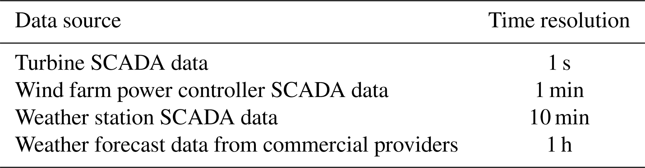
The proposed data-driven approach is based on multiple data sources: SCADA data from the wind turbines, from the wind farm power controller and from a weather station located in the wind farm, as well as weather forecasts from multiple weather forecast providers. Typically, such data sources have different time resolutions and accuracy levels. Measurement data from local measurements are typically more accurate than forecast data. Indeed, the accuracy of the former depends solely on the accuracy of the measurement instruments, whereas forecast data depend on large-scale models and observations with a wide spacial grid that may be wider than a complete wind farm. The time resolution of the data sources used for the showcases in this paper are shown in Table 1.
The optimal time resolution for a wind farm power model depends, on the one hand, on the purpose of the model (e.g. which effects are to be captured by the model) and, on the other hand, may be limited by the available computing hardware and required prediction speed. In order to capture the dynamics of a varying wind propagating through the wind farm, the time resolution of the model has to be sufficiently shorter than the duration needed by the wind to cross the entire wind farm. For example, for an offshore wind farm with a cross-section length of 10 km, with wind speeds between turbine cut-in and cut-out wind speeds of 4 and 30 m s−1, respectively, this duration is between 6 and 42 min. So, for that purpose, a sampling time of 1 min should be adequate. In addition, the farm power set point data available for this work has a 1 min time resolution, and so set point changes of the farm power controller can be captured as well.
In Sect. 2.1.1 to 2.1.4, each of the data sources used in the proposed methodology is described in more detail.
2.1.1 Turbine SCADA data
The turbine SCADA data of the wind farms that are used as showcases in this paper have a sampling time of 1 s. For both farms, the data of the turbines comprise the following measurements:
-
wind speed (measured by an anemometer located on top of the turbine nacelle),
-
wind direction (measured by a wind vane located on top of the turbine nacelle) and
-
turbine active power (measured at the power terminals of the turbine).
For one of the two farms, an additional data field is available which expresses the maximum power that the turbine could technically produce at a moment with sufficient wind:
-
turbine active-power capability.
The maximum power can indeed be limited below the rated turbine power due to a technical problem of the turbine or by a curtailment imposed from externally (e.g. by the farm power controller).
Based on the wind speed and direction measurement data, two additional data features are built that can be used as measures for the wind turbulence, wind turbulence intensity τ and wind direction variance ϕ, as
with σ(v) as the standard deviation of the wind speed; μ(v) as the average wind speed; and σ2(θlat) and σ2(θlon) as the variance of the lateral and longitudinal component of the wind direction, respectively, each during the 10 min time interval centred around the 1 s data point.
As the wind farm and the turbine power models proposed in this paper have a temporal resolution of 1 min, each of the above 1 s data feature sequences is averaged to 1 min data blocks.
2.1.2 Wind farm data
Most of the farm data can be calculated by aggregating the SCADA data from the individual turbines. The active power produced by the farm is calculated as the sum of the individual turbine active powers. Similarly, the farm active-power capability is calculated by summing up the power capability of each of the turbines.
Simply adding or averaging the wind measurement data of all individual turbines, however, would lead to a loss of information about the spatial variation in these features throughout the farm. Instead, the characteristics of the wind flowing into the wind farm are used, measured by a subset of turbines located in the upstream part of the farm. This also allows for isolating farm-internal wake and farm-external wake in separate ML models (the latter depending also on the operational status of the neighbouring farms). The set of upstream turbines is determined by the following algorithm for corrected geographic sorting (see Fig. 1):
-
calculate wind vector W as the average of the wind speeds and directions measured by all the turbines of the farm;
-
based on the farm layout, determine the projection of the position of each turbine on W;
-
select all turbines that are located in the most upstream zone of the farm with length D along W;
-
if the number of selected turbines is smaller than minimum number N, complete the set of turbines by adding additional turbines in the order of their projected position on W; and
-
from the set of N turbines, select the subset of M turbines with the highest wind speeds.
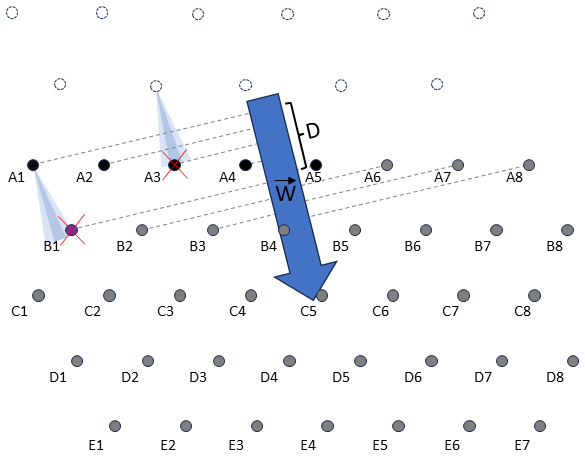
Figure 1Determination of the upstream turbines of the wind farm with turbines A1 to E7, for the case of an average wind W from the north-northwest direction. Turbines A1 to A5 are located in the most upstream zone of the farm with length D along W. As in this example the minimal number of upstream turbines to be taken into account (N) equals 6; turbine B1 is added to the set of upstream turbines. Finally, as in this example, the number of upstream turbines with the highest wind speed to be taken into account (M) equals 4; the two turbines with the lowest wind speed are not taken into account for determining the inflow wind characteristics. In this example, these are turbines A3 (which appears to be in a fully waked position from a turbine of a neighbouring wind farm) and B1 (which is in a partially waked position from turbine A1).
As a rule of thumb, an appropriate choice for parameter D is a value slightly smaller than the distance between the outer turbine rows of the farm. As a consequence, in the case that the wind vector W is nearly perpendicular to a side of the wind farm, all turbines in the upstream row will be selected as upstream turbines, enabling the capture of possible differences in wind characteristics over the complete width of the farm. In the case that the wind vector W is oriented towards a corner of the farm layout, however, only one single or very few turbines may be selected. Therefore, a minimum number N of turbines is selected, with N being a value which should be larger than 1 and smaller than the number of turbines in a single row. Finally, in order to remove turbines that risk being located in a narrow waked position caused by a turbine from the farm itself or from a neighbouring farm, only the M turbines with the highest wind speeds are retained. The farm inflow wind parameters (inflow wind speed, inflow wind direction, inflow turbulence intensity and inflow wind direction variance) are then calculated as averages of the corresponding features from the selected individual upstream wind turbines. The overall methodology presented in this paper can also be applied with alternative algorithms for determining the upstream turbines. There is, however, always a trade-off between the responsiveness of the model on wind transients and the average accuracy of the model, due to the spatial variation in the wind characteristics across the wind farm.
Note that the farm inflow wind characteristics, as determined by the above algorithm, are independent of the operational status of the wind farm and, in particular, of the control actions of the farm power controller. This is not the case for wind characteristics measured by turbines located in waked conditions more downstream in the wind farm. This independence makes it possible to map weather forecasts to the farm inflow wind characteristics with models that are independent of the wind farm operational status.
An additional farm parameter, having a major influence on the farm power production, is the set point of the farm power controller. Currently, for the majority of wind farms, active farm power control is still rarely used. Some farms, however, nowadays already use active farm power control in order to perform power balancing (Kölle et al., 2022). Due to the fast-growing share of wind energy in the energy mix, the use of farm power control may become more predominant in the near future. For the wind farms used as examples in this paper, the farm power set point data have a 1 min time resolution.
Finally, one additional wind farm feature is composed of the turbine SCADA data: the number of stopped turbines. If one or more turbines are stopped (e.g. for maintenance reasons), the total power of the farm is reduced. On the other hand, a turbine at standstill will not cause wake for other downstream turbines. Depending on the available turbine SCADA data of the farms, the feature “number of stopped turbines” is built by counting the number of turbines producing zero power (or even consuming power) or as the number of turbines with power capability equal to 0. Notice that, based on this feature, the farm power model does not get the information about which turbines specifically are at standstill, which may lead to some loss of accuracy in the model. Indeed, for example, stopping a turbine in a waked position may lead to less power reduction than stopping a turbine in an upstream position with free wind inflow.
2.1.3 SCADA weather data
For the showcases in this paper, measurement data from a weather station located in one of the wind farms are used. The data set comprises the air temperature, humidity and pressure. Based on these three measurements, the relative air density is calculated. For the farms used as examples in this paper, the available measurements are data averaged over 10 min intervals. In order to use the air density as input for the 1 min farm and turbine power models, the data series is interpolated to a 1 min data sequence.
2.1.4 Weather forecast data
For the showcases in this paper, wind speed and direction forecasts have been used for the location of the wind farms and for a height of 100 m (similar to the hub height of the turbines). The forecasts are provided by a commercial weather forecast provider and have a 1 h time resolution. Based on the lead time of the forecasts, separate data sets have been composed with intra-day forecasts, day-ahead forecasts (before 11:00 the day before energy production) and 3 d ahead forecasts.
2.2 Multi-component pipeline
Figure 2 shows the overall modular structure of the methodology proposed in this paper, integrating the components described in Sect. 2.3 and 2.4. Weather forecasts of weather forecast providers are processed as forecasts of the wind inflow experienced by the farm. In doing so, phenomena such as external wake, wind farm blockage, coastal effects and other unknown systematic forecasting errors are accounted for. Based on these corrected inflow wind speeds and directions, possibly unknown wind parameters are estimated using auxiliary models. With all the resulting input parameters, the wind farm power is forecasted. Additionally, the power of an individual turbine operating under identical environmental conditions is forecasted. By subtracting the power forecast of the wind farm from the power forecast of the individual turbine multiplied by the number of turbines in the farm, the wake loss within the wind farm can be quantified.
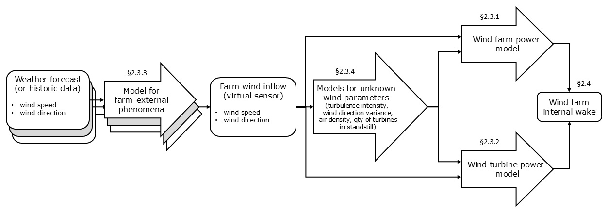
Figure 2Overview of the modular structure of the multi-component pipeline with multiple ML models.
2.3 Machine learning models
In this section, all ML models are described which are part of the modular deep learning pipeline (Sect. 2.2). The wind farm power model, which is the core model of this work, is detailed in Sect. 2.3.1. This model predicts the real-time wind farm power production based on a set of wind inflow measurements and other farm-specific parameters. The ML model for predicting the real-time power of an individual wind turbine is presented in Sect. 2.3.2. The models for converting weather forecasts into accurate forecasts of the wind inflow conditions experienced by the wind farm are detailed in Sect. 2.3.3. Lastly, the auxiliary models used to estimate missing input parameters for the wind farm and turbine power models are discussed in Sect. 2.3.4.
2.3.1 Wind farm power ML model
The core ML model proposed in this paper predicts the wind farm power based solely on measurement data from conventional turbine instrumentation. This type of data is usually available to any wind farm operator. Each of the input features of the model has a direct (physical) influence on the power production of the wind farm.
As it typically takes between several minutes and half an hour for the wind to cross a complete wind farm (depending on the wind speed and size of the farm), the wind and wake characteristics at time ti across the farm depend not only on the wind inflow at time ti but also on the evolution of the wind inflow between ti and ti−T (with T=30 min). Also control actions from the farm power controller and the number of stopped turbines in the past may have an influence on the spatial wind and wake profile across the farm. In contrast, some input parameters have an immediate discontinuous impact on the farm power production, independent of their historical values. For example, a farm power controller can quasi-instantaneously (i.e. with a response time smaller than or similar to one 1 min time step) reduce the power of all turbines across the wind farm. Therefore, the proposed model is composed of two separate parts. For each input parameter that influences the wind and wake profile across the farm in a continuous way, a sequence of historic values is passed to a convolution branch. The outputs of these convolution branches are then passed to a feed-forward neural network, together with the input parameters that have (only) an immediate impact on the wind farm power production.
The structure of the proposed farm power model is shown in Fig. 3. K separate convolution branches consist of two 1D convolutional layers. The outputs of these K branches are passed, together with L additional input features, through a flattening and dropout layer, to a feed-forward regression neural network composed of three dense layers, each followed by a dropout layer. Each convolution layer has eight convolution filters () with a kernel size of 3, a stride of 1 and no padding. The fully connected dense layers have 128 (n1), 256 (n2) and 256 (n3) units with a rectified linear (ReLU) activation function, respectively.
A feed-forward neural network is one of the simplest types of artificial neural networks, where the information flow is in one direction, from the input layer, passing through the hidden layers to the output layer. A dense layer is a fully connected layer where every neuron in the layer is connected to every neuron in the previous layer. A convolution layer involves the sliding of filters over the input data. A filter is a small matrix with learnable parameters. In the proposed model, each filter, with a dimension of 1×3 (kernel size), slides with a step of 1 (stride step) over the input time sequences and can detect specific patterns in these sequences that are significant for the farm power production. A flattening layer is a layer which transforms a multi-dimensional array into a 1D array. A dropout layer is a layer in which randomly a fraction of the neurons outputs are set to 0 during training, and so effectively neurons drop out of the network. This prevents the network from becoming overly reliant on specific neurons, which reduces overfitting and improves the robustness of the model. A rectified linear activation function is one of the most widely used activation functions in neural networks, which introduces non-linearity in the network to allow the model to learn complex patterns.
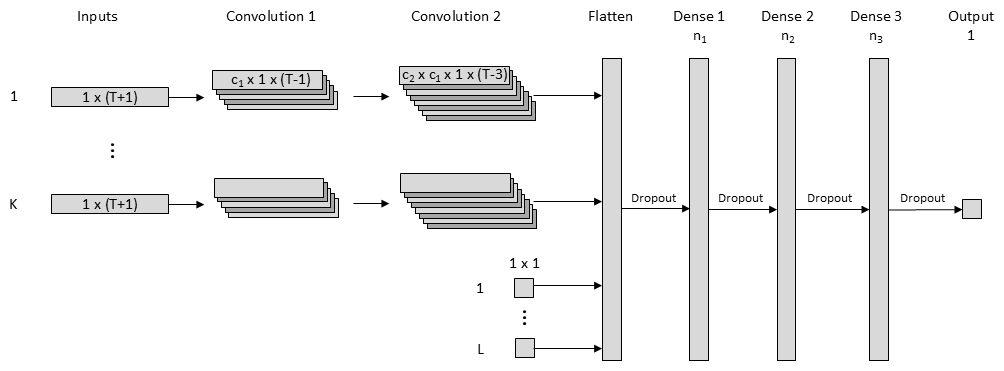
Figure 3Structure of the proposed deep learning farm power model. K separate convolution branches consist of two 1D convolutional layers. The outputs of these K branches are passed, together with L additional input features, through a flattening and dropout layer, to a three-layer regression model that is composed of three dense layers, each followed by a dropout layer.
Time sequences from ti to ti−T of the following K input parameters (based on SCADA data) are passed to the K convolution branches:
-
farm inflow wind speed,
-
lateral component of the farm inflow wind direction,
-
longitudinal component of the farm inflow wind direction,
-
farm inflow turbulence intensity (Eq. 1),
-
farm inflow wind direction variance (Eq. 2),
-
air density,
-
set point of the farm power controller (if available in the data set),
-
number of stopped turbines and
-
active-power capability of the farm (if available in the data set).
In parallel, the values at ti of the following L input parameters are passed directly to the feed-forward component of the neural network:
-
set point of the farm controller (if available in the data set),
-
number of stopped turbines and
-
active-power capability of the farm (if available in the data set).
Notice that the lateral and longitudinal components of the wind direction are used as inputs, instead of the wind direction itself (expressed in degrees). This is done to guarantee continuity in the data for the wind direction 360° (0°).
The dropout layers in the neural network model allow for not only predicting the expected power production of the wind farm but also quantifying the uncertainty in that prediction. The method applied in this paper is referred to as Monte Carlo dropout (Gal and Ghahramani, 2016). This is an epistemic method as it quantifies the uncertainty arising from the model architecture and the amount of data.
Instead of generating one single prediction of the farm power for time step ti, N′ different power predictions are generated using the model with active dropout layers (in the same way as during the training phase of the model). The power prediction is then calculated as the average of these N′ different power predictions. In addition, also the variance of these N′ power forecasts can be determined, as well as an arbitrary set of percentiles and thus confidence intervals .
Unfortunately, the Monte Carlo dropout method is prone to miscalibration; i.e. the predictive uncertainty does not correspond well to the model error. Therefore, a method referred to as sigma scaling is applied, jointly calibrating the epistemic uncertainty from the model and the aleatoric uncertainty from the data (e.g. due to sensor noise) (Laves et al., 2020). For each time step ti of the test data set, the following ratio is calculated:
with Pi as the true farm power at time step ti. According to Eq. (3), is thus the ratio of the prediction squared error of the model for time step ti and the variance calculated with the Monte Carlo dropout method for that time step. Analysis of the results for the wind farms used as example in this paper shows that the prediction errors and ratios depend mainly on the wind speed and the set point of the farm power controller. This could be expected, as for low wind speeds and for high wind speeds above the rated turbine wind speed, the power curve of the turbines is relatively flat. In contrast, for wind speeds slightly below the rated wind speed, the power curve of the turbines is the steepest. Therefore, a calibration function q2(v,s) is established, with the wind speed v and the set point of the farm power controller s. This is done by mapping a simple feed-forward neural network (with two hidden dense layers with 256 units) to the complete test data set. With this calibration function, the variance predicted with the Monte Carlo dropout method is re-calibrated as
Similarly, the confidence intervals generated with the Monte Carlo dropout method are re-scaled as
2.3.2 Turbine ML model
Based on the same data set as that used for the farm power model, a turbine power model is also built. This turbine model has thus also a 1 min time resolution. However, in order to model a healthy turbine without any technical deration, a reduced power mode or curtailment by its power controller, all data points with a reduced power capability and/or curtailment are removed from the training data set.
In contrast to a wind farm, the power production of a single turbine does not depend on the wind speed from multiple antecedent 1 min time steps. Indeed, the response time of a single wind turbine, which is determined predominately by the inertia of its rotor, is significantly faster. Furthermore, the wind direction has no direct influence on the power of a turbine, as long as the yaw control system orientates the turbine perpendicular to the incoming wind direction (for the wind farms used as examples in this paper no wake steering is done by applying yaw control).
As input data features, wind speed, turbulence intensity (Eq. 1), wind direction variance (Eq. 2) and air density are used. The turbine power is modelled by a simple feed-forward neural network, composed of three fully connected dense layers, each with 128 units with a rectified linear activation function.
2.3.3 ML models for mapping weather forecasts
Commercial weather forecast services nowadays provide weather forecasts for specific geographical locations, such as the position of a wind farm. Forecasts of different providers can differ due to the use of different weather models or data. Usually, wind speed and wind direction forecasts do not take into account the presence of neighbouring wind farms or coastlines. Furthermore, the forecasts may not have exactly the same calibration as the instrumentation that has been used to train the wind farm power model.
Therefore, the weather forecasts should be mapped to the real weather conditions experienced by the wind farm. The appropriate data-driven models for such mappings will depend on the available data sources from weather forecast providers. For the showcases in this paper, the wind speed forecasts are mapped to the measured farm inflow wind speeds and the wind direction forecasts are mapped to the measured farm inflow wind directions.
The structure of the ML model that is used for the wind speed mapping is shown in Fig. 4 (left). It is a feed-forward regression neural network with three hidden dense layers, each followed by a dropout layer. The dense layers consist of 16 (n1), 32 (n2) and 32 (n3) units with a ReLU activation function, respectively. As the time step of the weather forecasts available for this work are rather course (1 h time step), in a pre-processing step, the 1 h wind speed forecast data are first interpolated to wind speed forecast data with a 10 min time step. In order to provide the mapping model the possibility of capturing the possible influence of wind speed variations, not only the wind speed forecast of the specific 10 min time step but also the wind speed forecasts of the two preceding and the two following 10 min times steps () are used as an input feature. As an output feature, the average inflow wind speed vt for the 10 min time step is used.
The structure of the ML model used for the mapping of the wind direction forecasts is the same as for the wind speed forecasts. The only differences are the input and output features, which are the cosine and sine of the forecasted and measured wind directions, , , cos θt and sin θt, respectively. The structure of the ML model is shown in Fig. 4 (right).
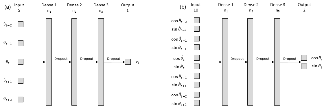
Figure 4Structure of the deep learning models used to map wind speed forecasts to measured inflow wind speeds (a) and wind direction forecasts to measured inflow wind directions (b).
2.3.4 Auxiliary ML models for missing input parameters
The farm power model (as specified in Sect. 2.3.1) has many input parameters related to the inflow wind. Sometimes the value of some of these wind characteristics is not known, at least not accurately. For example, weather forecast providers usually do not provide accurate information about the wind turbulence when also taking the presence of neighbouring wind farms into account. In such a case, one could decide to use a single average value for these parameters. However, the turbulence intensity, wind direction variance, air density and the number of stopped turbines depend all more or less on the wind speed and wind direction. Therefore, for each of these four parameters a model is built to predict its value based on the wind speed and wind direction. These auxiliary models may be specific for a particular wind farm and are not the focus of this paper.
2.4 Farm-internal wake loss
The proposed modular approach also allows for predicting the power losses in the wind farm due to internal wake (see Fig. 2). The power loss in a wind farm with J wind turbines due to internal wake can be calculated as
with as the power production of wind turbine j subjected to wind with the same characteristics as the inflow wind of the farm and P as the farm power. In the case of J identical turbines, the farm power loss due to wake can be simplified as
Consequently, the wake loss can be modelled using the wind farm power model (as proposed in Sect. 2.3.1) and the model for a single turbine (Sect. 2.3.2):
with v, θ, τ, ϕ and ρ, respectively, as the farm inflow wind speed, wind direction, turbulence intensity, wind direction variance and air density. Notice that for the farm power model, and thus also for the wake model, these wind parameters are 30 min time sequences.
2.5 Baseline models
In order to demonstrate the influence of some key implementation choices of the wind farm power model (Sect. 2.3.1), its performance metrics are compared with those of two baseline models that do not comprise these implementation choices.
The first baseline model is a feed-forward neural network model with three hidden dense layers, which is a sub-component of the proposed wind farm power model. This baseline model, however, does not comprise any convolution layer and takes only the wind speed and the sine and cosine of the wind direction at time step t0 as input features. Consequently, this model has no information about the preceding 30 min and, by consequence, no information about the variability in the wind parameters. Furthermore, this model has no knowledge about the other measurement data, such as the air density, turbulence intensity and wind direction variation, nor about the farm power controller and the number of turbines at standstill.
The second baseline model is identical to the proposed wind farm power model, with the exception that it does not comprise any convolution layer. This baseline model has the same set of input features as the wind farm power model, but, similar to the other baseline model, it does not have information about the variability in the wind parameters.
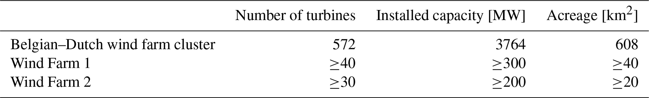
The methodology as described in Sect. 2 has been applied to two offshore wind farms located in the Belgian–Dutch wind farm cluster in the North Sea (see Fig. 5). This cluster comprises 13 wind farms. It is located at a distance of 20 to 60 km from the Belgian and Dutch coastline. For confidentiality reasons, the two wind farms are denoted in this paper as Wind Farm 1 and Wind Farm 2. The two farms are operated by different farm operators and have a different type of wind turbine. The main characteristics of the two farms and the complete wind farm cluster are listed in Table 2. All presented results involving farm power and turbine power are normalized with the installed capacity of the wind farm and the rated turbine power, respectively.
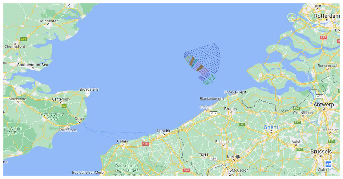
Figure 5Position of the Belgian–Dutch offshore wind farm cluster in the North Sea (© Google Maps).
Table 2Main characteristics of the Belgian–Dutch offshore wind farm cluster and the two wind farms used as examples in this paper.
The results are grouped into the following three sections. In Sect. 3.1, results are presented as being related to the core wind farm power prediction model of each of the two wind farms. Section 3.2 focuses on the estimation of farm-internal wake. Finally, in Sect. 3.3, some results are shown as being related to the integration of weather forecasts.
3.1 Wind farm power model
3.1.1 Data
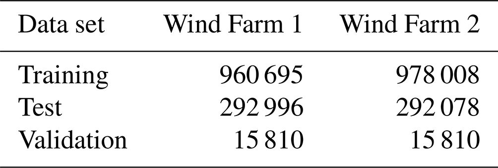
For both Wind Farm 1 and Wind Farm 2, weather and turbine data were available for a period of about 2.5 years. Table 3 shows the number of 1 min data points resulting from the pre-processing of the SCADA data, which were split into distinct training, test and validation data sets.
For splitting the available data into three independent data sets, the following steps have been applied. First, a long time sequence of consecutive days is selected as the validation data set. Thereafter, in order to guarantee that the test and training data sets are sufficiently independent and, at the same time, are both representative of all seasons, hours of the day and days of the week, the test data set is established by selecting all data from some days of the month from the remaining data. More specifically, the test data set comprises the data from days 2, 3, 4, 16, 17, 18 and 28 of each month.
Table 3Number of data points used for training, testing and validating the two wind farm power models.
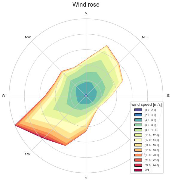
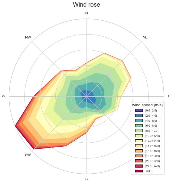
Figures 6 and 7 show the wind roses for the inflow wind of Wind Farm 1 and Wind Farm 2, respectively. South-southeast is the predominant wind direction with also the highest wind speeds. Although the two wind farms are located close to each other in the same wind farm cluster, the wind conditions experienced by the two wind farms are different.
The data plots in Figs. 8, 10 and 12 illustrate the dependency of the farm power on the wind turbulence intensity, wind direction variance and air density, respectively. Higher wind turbulence results in higher farm power, as higher turbulence facilitates the wake recovery, thus reducing the possible power loss for downstream turbines. Higher air density also results in an increase in the turbine power because the mass, and thus kinetic energy, of the moving air is higher.
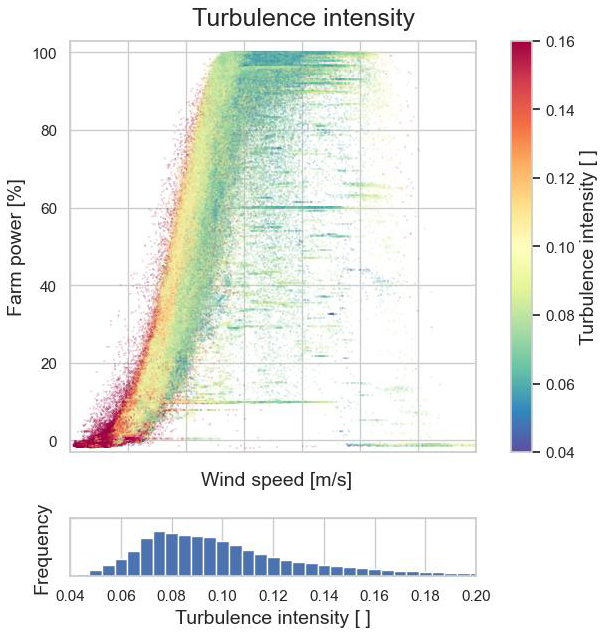
Figure 8Farm power as a function of inflow wind speed and wind turbulence intensity and the frequency distribution of turbulence intensity (Wind Farm 2).
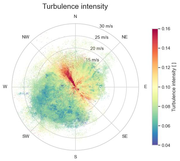
Figure 9Inflow turbulence intensity as a function of wind speed and wind direction (Wind Farm 2).
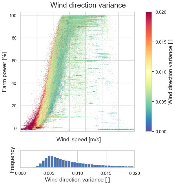
Figure 10Inflow wind direction variance as a function of wind speed and wind direction and the frequency distribution of wind direction variance (Wind Farm 2).
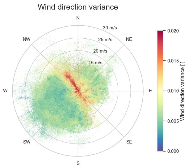
Figure 11Inflow wind direction variance as a function of wind speed and wind direction (Wind Farm 2).
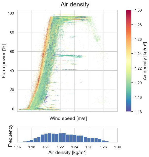
Figure 12Farm power as a function of inflow wind speed and air density and the frequency distribution of air density (Wind Farm 1).
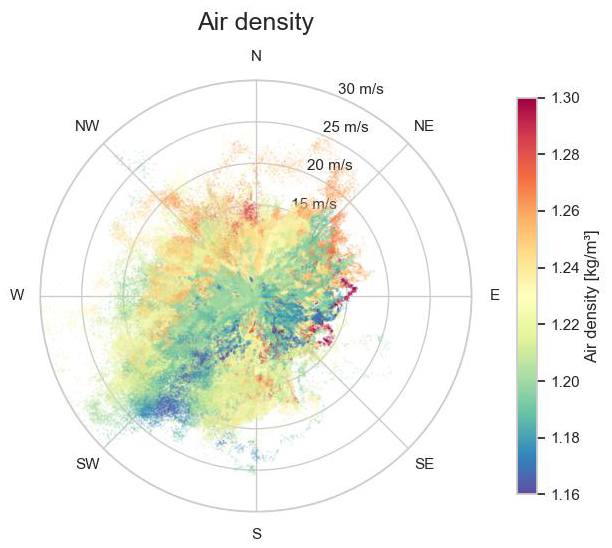
The polar data plots in Figs. 9, 11 and 13 give an indication of the correlation between turbulence intensity, wind direction variance and air density with the inflow wind speed and wind direction, respectively. In the northwest and southeast wind directions, Wind Farm 2 has neighbouring wind farms with densely positioned turbines in its immediate vicinity, resulting in a high turbulence intensity for these wind directions. Also in the northeast direction, Wind Farm 2 has a neighbouring wind farm. However, that wind farm is located further away and its turbines are positioned less densely. It can also be seen that the wind turbulence is lower for high wind speeds than for slow speeds. Furthermore, it can be seen that the southwest direction is the wind direction with the highest wind speeds. In that direction, the wind is coming from over sea parallel to the coastline, through the narrow Strait of Dover, which has high cliffs. It can also be seen that wind parallel to the coastline typically has a lower air density compared to the orthogonal directions from and to the mainland. This corresponds to the fact that humid air has a lower air density than dry air.
When comparing Figs. 8 and 12 from Wind Farm 2 and Wind Farm 1, respectively, it can be seen that Wind Farm 2 has markedly more data points with a reduced power. This is due to the power controller of the wind farm which, in some circumstances, regulates the farm power in a continuous manner. In contrast, for Wind Farm 1, there appear to be farm curtailments to a few specific discrete power set points (such as ∼ 60 % of the maximum farm power). Furthermore, it can also be seen that for Wind Farm 1 the total installed turbine capacity is never reached. This is due to the farm power controller, which limits the maximum producible power of the farm.
3.1.2 Hyper-parameters
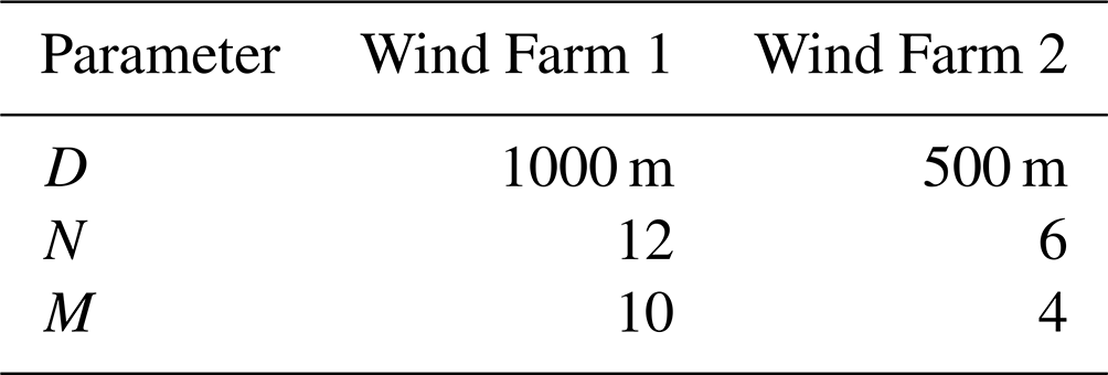
Table 4 shows the parameters used to determine the set of upstream turbines according to the algorithm described in Sect. 2.1.2. Wind Farm 1 comprises more turbines than Wind Farm 2 (parameter N), and these are positioned more widely apart (parameter D).
Table 4Parameters used for the selection of the upstream turbines.
The hyper-parameters of the wind farm power ML model (Sect. 2.3.1) and of the wind forecast mapping ML models (Sect. 2.3.3) are documented in Appendix A.
3.1.3 Performance metrics
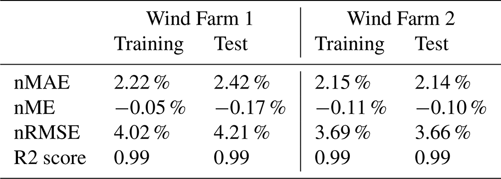
In Table 5, some performance metrics (Piotrowski et al., 2022) of the farm power models for Wind Farm 1 and Wind Farm 2 are listed: the root mean square error normalized on the installed power capacity of the wind farm (nRMSE), the normalized mean absolute error (nMAE), the normalized mean error (nME) and the R2 score, for both the training and test data set. The nME for each of the farms is near to 0 %, and the nMAE is 2.42 % and 2.14 % for the test data sets of Wind Farm 1 and Wind Farm 2, respectively. The differences between the performance metrics of the training and test data sets are very small, which is a sign for a satisfactory fit (little overfitting).
Table 5Performance metrics of the power models for Wind Farm 1 and Wind Farm 2.
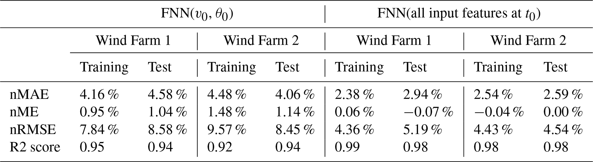
In Table 6, as a comparison basis, the corresponding performance metrics are shown for the two baseline models described in Sect. 2.5. FNN(v0,θ0) (feed-forward neural network) denotes the first baseline model, which has only the inflow wind speed v0 and the sine and cosine of the inflow wind direction θ0 at time step t0 as input features. FNN(all input features at t0) denotes the second baseline model, which equals the proposed wind farm power model but without convolution layers. It has the same set of input features but only for time step t0. Comparing the performance metrics of the wind farm power model proposed in this work (Table 5) with those of the two baselines models (Table 6), one can see, for example, that for the test data the nMAE is reduced by about 47 % and 18 %, respectively (for both wind farms). Thus, both the usage of additional input parameters (among others, turbulence intensity, air density and the set point of farm power controllers) and information from the preceding time period (30 min) improve the performance of the farm power model significantly. Note that none of the baseline models can capture the dynamics caused by variable wind inflow.
Table 6Performance metrics for two baseline deep learning power models for both Wind Farm 1 and Wind Farm 2.
Figures 14 and 15 give some insight into the prediction error for individual test data points. It can be seen that the prediction error is the smallest for conditions where the farm power is close to 0 % or 100 % of the installed capacity. Indeed, these regions comprise many data points with wind speeds below the turbine cut-in wind speed and wind speeds above the rated turbine wind speed, where the power curve of the turbines is relatively flat, respectively.
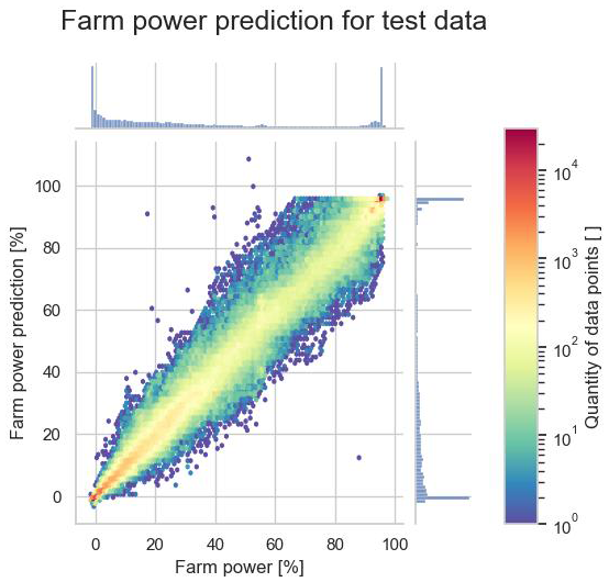
Figure 14Relation between predicted and true farm power for all data points of the test data set for Wind Farm 1.
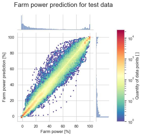
Figure 15Relation between predicted and true farm power for all data points of the test data set for Wind Farm 2.
3.1.4 Validation time sequence
Figure 16 shows the predicted and true farm power for a 60 h time sequence of validation data for Wind Farm 1, as well as the predicted confidence intervals. The confidence intervals are the smallest for high wind speeds resulting in maximum farm power and for low wind speeds with a farm power close to 0 MW. The uncertainty appears to be the highest when the farm power is fluctuating and peaking heavily. In contrast, for long continuous power increases or decreases, the predicted uncertainty in the model appears to be relatively low. For this time sequence, 69.0 % of the 1 min true farm power data points lay within the 68.3 % confidence interval and 97.5 % of the data points lay within the 95 % confidence interval (when ignoring the true farm data points at maximum and zero farm power, where the absolute prediction error is negligible).
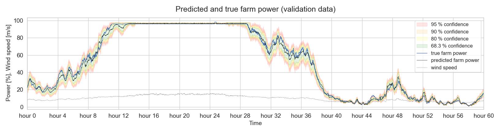
Figure 16Predicted farm power and uncertainty intervals for a 60 h time sequence of validation data (Wind Farm 1).
Figure 17 shows the predicted and true farm power for a time sequence of test data during which the farm power controller of Wind Farm 2 is actively curtailing the farm power (i.e. the set point of the power controller is smaller than 100 %). The uncertainty in the model appears to be very low when the wind speed is largely sufficient to attain the power set point.
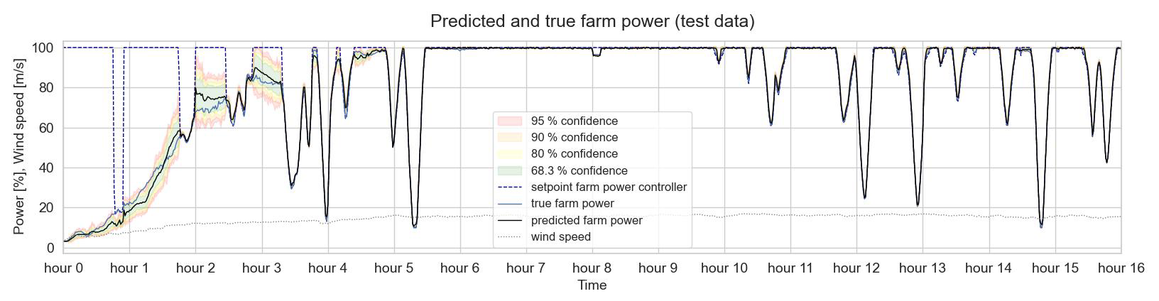
Figure 17Predicted farm power and uncertainty intervals for a 16 h time sequence of test data with active-power control (Wind Farm 2).
3.1.5 Sensitivity analysis
Figures 18 to 23 illustrate the sensitivity of the farm power curve generated by the farm power model for each of the input parameters. In each of the plots, the farm power is shown as a function of the wind speed. The other input parameters are predicted by the corresponding auxiliary models (see Sect. 2.3.4) based on the wind speed and a specific wind direction. One single input parameter is then adapted slightly in order to analyse the resulting impact on the predicted farm power. Each simulation is a steady-state simulation; i.e. the value of each of the input parameter sequences is constant in time.
Figures 18 to 20 show that the models predict a higher farm power for an increased turbulence intensity, wind direction variance and air density, respectively. This confirms what can be seen in Figs. 8, 10 and 12. Figure 21 shows the predicted power for Wind Farm 1 for two different wind directions. The produced power for a wind direction of 240° is lower than for a wind direction of 180°. This difference is due to farm-internal wake (see also Sect. 3.2). Indeed, a wind direction of 240° is parallel to a long cross-section of Wind Farm 1. In contrast, a wind direction of 180° is slightly off the short cross-section of the wind farm. For this wind direction, the internal wake is thus minimal. Figure 22 shows the predicted power reduction for Wind Farm 2 when one and two turbines, respectively, are stopped. As mentioned in Sect. 3.1.1, the maximum power of this wind farm is limited by its farm controller. As can be seen in Fig. 22, at high wind speeds this maximum power limit can almost be reached with one turbine at standstill. Figure 23 shows the farm power for Wind Farm 2 in the case that the set point of the farm power controller equals 30 %, for the wind directions of 325° and 260°. For low wind speeds, the farm power for a wind direction of 260° is lower than for one of 325° because of the higher farm-internal wake.
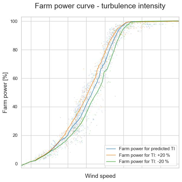
Figure 18Predicted farm power as a function of inflow wind speed and wind turbulence intensity (TI) (Wind Farm 2).
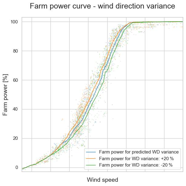
Figure 19Predicted farm power as a function of inflow wind speed and wind direction (WD) variance (Wind Farm 2).
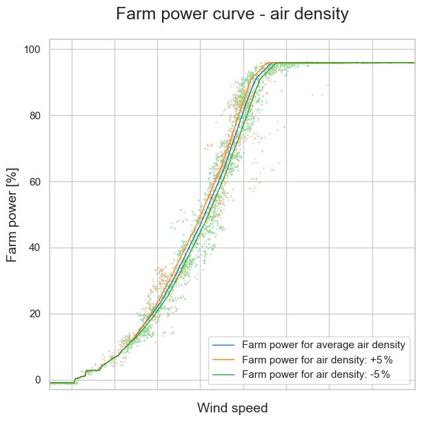
Figure 20Predicted farm power as a function of inflow wind speed and air density (Wind Farm 1).
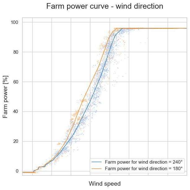
Figure 21Predicted farm power as a function of inflow wind speed and wind direction (Wind Farm 1).
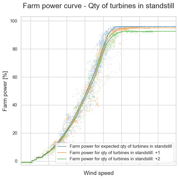
Figure 22Predicted farm power as a function of inflow wind speed and the number of turbines at standstill (Wind Farm 1).
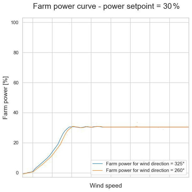
Figure 23Predicted farm power as a function of inflow wind speed and direction, with the farm power controller set point equal to 30 % (Wind Farm 2).
3.1.6 Farm power dynamics
All power predictions presented in Sect. 3.1.5 are for steady-state conditions; i.e. all input parameters of the model are constant, at least during the last thirty-one 1 min time steps , which are input features of the farm power prediction model. As explained in Sect. 2.3.1, the structure of the neural network of the farm model has been chosen specifically to be able to capture temporal variations in the inflow wind characteristics. In this section, the farm power is predicted for wind speeds that fluctuate over time. The objective is twofold: firstly, to assess the ability of the model to predict consistent and physically meaningful results under these dynamic conditions and, secondly, to gain insights into how wind speed variations impact farm power production, which cannot be modelled by traditional steady-state power models. Two types of wind speed variations are tested: linear wind speed ramps and sinusoidal varying wind speeds with different frequencies.
Figure 24 shows power predictions for Wind Farm 1 for the same wind directions as shown in Fig. 21 (i.e. 150 and 240°). However, in addition to the two power curves for constant wind speeds (), power predictions are shown for the cases with a linear wind speed increase and decrease with a change rate of 0.05 m s−1 min−1 (i.e. m s−1 and m s−1, respectively). It can be seen that in the case of increasing wind speed (dashed lines), the predicted farm power is lower. In contrast, for decreasing wind speed (dotted lines), the predicted power is higher. Indeed, if at the inflow side of the wind farm the wind speed is increasing, in the downstream in the wind farm the wind speed is still lower than at the inflow side, resulting in a lower total farm power. As can be seen on this plot as well, this effect is larger for a wind direction of 240° (blue arrows) than for a wind direction of 180° (orange arrows). This is because the cross-section of the wind farm with a wind direction of 240° is longer than that with a wind direction of 180°. Consequently, changed wind speeds need more time to reach the downstream turbines. In addition, on the plot it can be seen that there is a hysteresis for the startup and shutdown of the turbines around the cut-in wind speed. Note that for static wind farm power models, in Fig. 24, all curves for a wind direction of 150° would be identical and all curves for a wind direction of 240° would be identical.
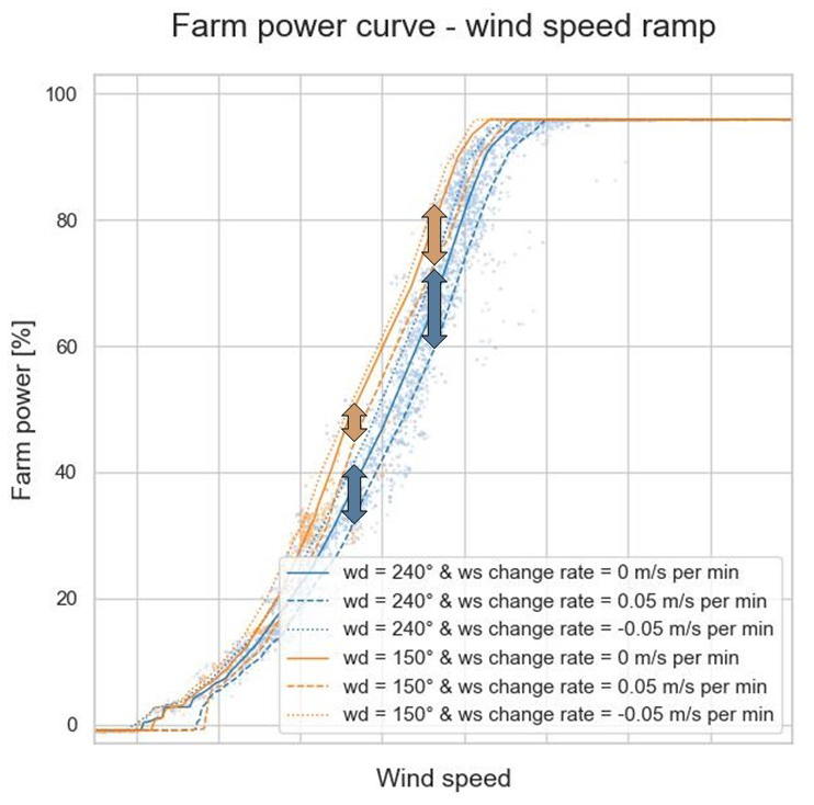
Figure 24Predicted farm power as a function of inflow wind speed (WS) with a linearly increasing and decreasing speed with a change rate of 0.05 m s−1 min−1, for the wind direction (WD) at 240 and 150° (Wind Farm 1).
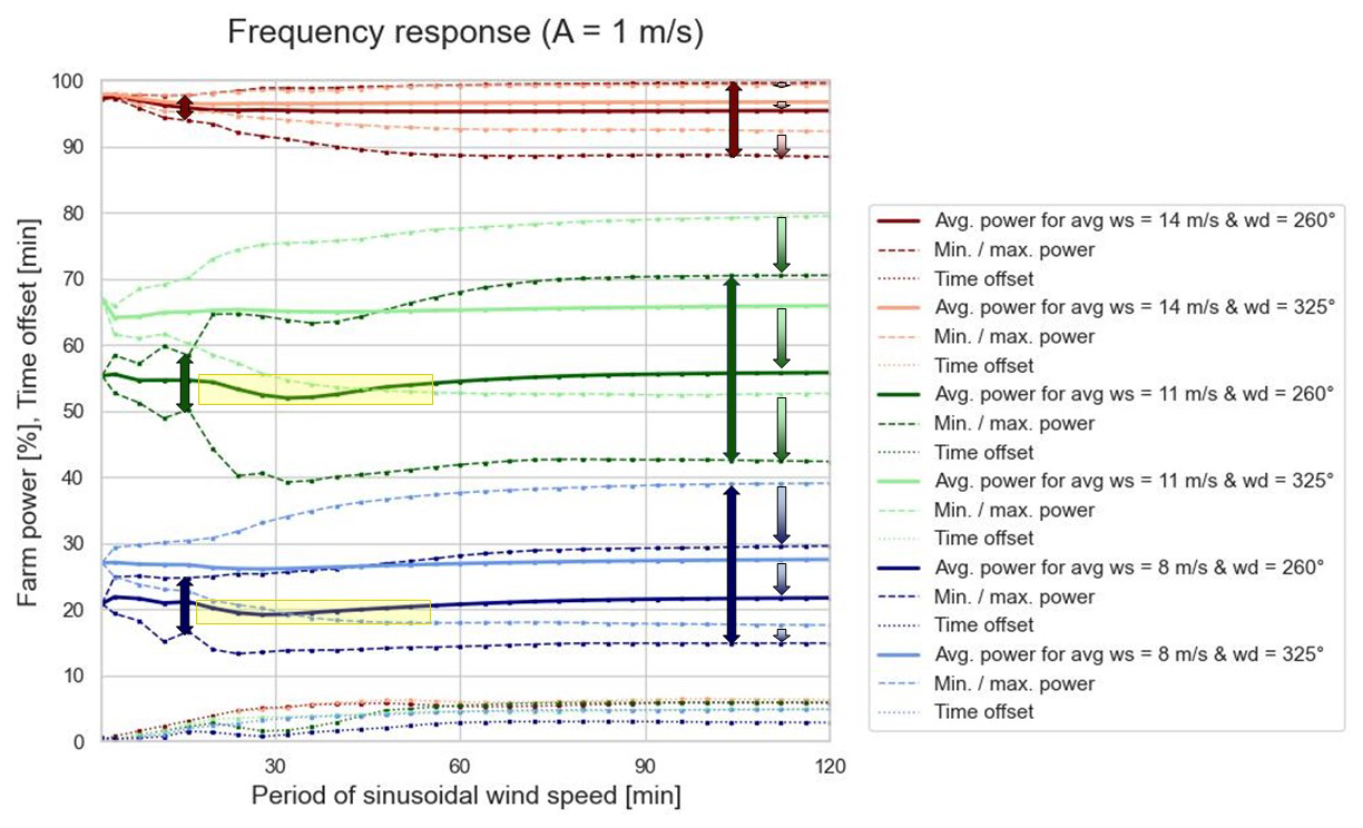
Figure 25Frequency response of predicted farm power in the case of a wind inflow with a sinusoidal oscillating wind speed component with an amplitude of 1 m s−1. The plots show the average, maximum and minimum power of the predicted oscillating farm power as a function of the period of the sinusoidal component of the wind speed. In addition, also the time offset between the oscillating farm power and wind speed is shown. The colour of the curves indicates the average wind speed (14, 11 and 8 m s−1, respectively) and the wind direction (260 and 325°) (Wind Farm 2).
Figure 25 shows the frequency response of the power model for Wind Farm 2. The inflow wind speed is simulated as a constant average speed V superposed with a sinusoidal component with an amplitude of 1 m s−1 ()). Simulations were run for a period T of the sinusoidal component equal to 2 to 120 min ( min). This has been done for different average wind speeds (V=14, 11 and 8 m s−1) and wind directions (260 and 325°). The curves show the average, maximum and minimum values of the resulting oscillating farm power (solid and two dashed lines), as well as the time delay between the sinusoidal wind speed component and the oscillating farm power (dotted lines).
As an oscillation period of 120 min is much longer than the time needed for the wind to cross the complete wind farm, which is a quasi-static wind condition. For smaller oscillation periods, the frequency of the wind oscillations is higher. However, for T=2 min, taking into account the 1 min time step, the wind speed is again constant (because ).
As can be seen on the plot, for a specific wind speed and oscillation frequency, the average, maximum and minimum farm power for a wind direction of 260° (with high wake) is always lower than for a wind direction of 325° (with less wake) (see downward arrows). For faster-fluctuating wind speeds (i.e. with shorter oscillation period), the amplitude of the farm power fluctuation decreases (see bidirectional arrows). In addition, in the case of wind conditions with a high farm-internal wake, there appears to be a decrease in the average farm power (see yellow markings). For small oscillation periods below 15 min, the average power increases again, converging back to the same value as for quasi-static wind conditions.
For short oscillation periods and consequently small wavelengths of the spatial wind speed distribution, the time delay of the farm power converges to 0. Indeed, the time delay cannot be longer than the oscillation period of the sinusoidal wind speed component. For longer oscillation periods, the time offset converges to a constant value. Logically, the time delay will never be higher than the time needed by the wind to cross the whole farm.
For short oscillation periods below 15 min, the wavelength of the wind speed oscillation gets smaller than the cross-section of the farm. This may cause the important decrease in the amplitude of the farm power oscillation. This might also explain the jigsaw shape of the maximum and minimum power in these conditions. To analyse these effects in more detail, a wind farm model could be used that predicts not only the total farm power but also the power production of each individual turbine.
Note that for static wind farm power models, all curves in Fig. 25 would be horizontal lines and be equal to the values for the longest shown oscillation period (T=120 min).
The analysis in this section is a qualitative analysis. As the simulations are done with fictive wind speeds, there are no ground-truth values for the farm power production to compare with. Note, however, that the performance metrics presented in Table 5 are for measured wind data and thus cover realistic wind speed variations. These performance metrics thus cover the dynamic behaviour of the farm power model.
3.2 Farm-internal wake
As already shown in Fig. 21, the farm power production depends on the wind direction due to the difference in wake loss. In order to calculate the farm-internal wake in absolute terms, an ML model has been established for a single turbine, as described in Sect. 2.3.2. By subtracting the power predicted by the farm power model from the predicted turbine power under identical wind conditions (multiplied with the number of turbines in the farm), the farm-internal wake effect can be isolated from other influences on the farm power.
Figure 26 shows the measured farm power for Wind Farm 1, as a function of the wind direction and wind speed. Figure 27 shows the subset of these data points for which the set point of the farm power controller is equal to 100 % and at maximum one turbine is at standstill. Furthermore, the scope of the plot has been limited to the wind speed range for which wake is most predominant. Figure 28 shows the corresponding predicted farm power by the farm model for steady-state wind inflow (for 30 min). It can be seen that for the west-southwest and east-northeast directions for a given wind speed, the farm power is lower than for other wind directions. This can be seen more clearly after subtraction from the predicted turbine power. Figure 29 shows the power loss due to internal wake as a percentage of the installed capacity of the farm. The maximum internal wake loss is about 30 %. The reason for the high wake in the west-southwest and east-northeast directions is that these directions are parallel to the long axis of the wind farm, with multiple turbines positioned after each other. For wind speeds above 13 m s−1, the power loss due to wake approaches 0 MW. This is because at such high wind speeds there is sufficient energy in the wind, and consequently each turbine in the farm can produce sufficient power so that the maximum farm power is reached.
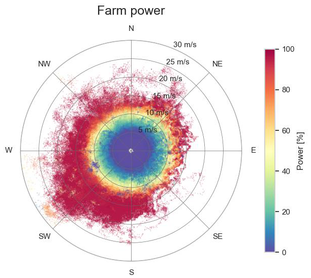
Figure 26Farm power measurement data points as a function of wind speed and direction (Wind Farm 1).
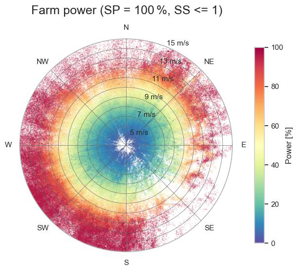
Figure 27Subset of farm power measurement data points as a function of wind speed and direction, with the farm power control set point (SP) equal to 100 % and number of turbines at standstill (SS) equal to 0 or 1 (Wind Farm 1).
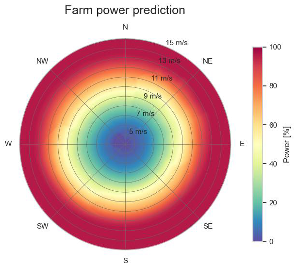
Figure 28Predicted farm power as a function of wind speed and direction, for constant wind conditions, with the farm power control set point equal to 100 % and with all turbines in operation (Wind Farm 1).
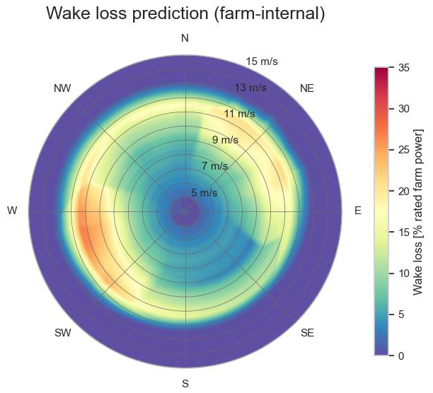
Figure 29Predicted farm-internal wake as a function of wind speed and direction, for constant wind conditions, with the farm power control set point equal to 100 % and with all turbines in operation (Wind Farm 1).
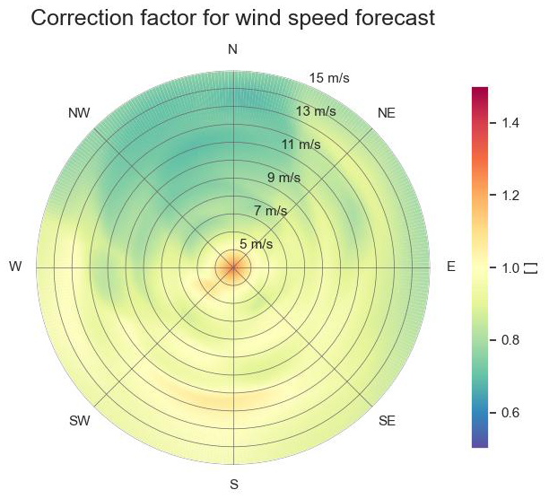
Figure 30Correction factor for the wind speed forecasts of a weather forecast service for Wind Farm 1.
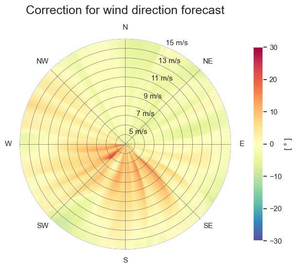
Figure 31Correction for the wind direction forecasts of a weather forecast service for Wind Farm 1.
3.3 Power forecasting based on weather forecasts
The farm power prediction models presented in Sect. 3.1 and 3.2 predict the farm power based on measurement data of the wind inflow and some other parameters of the farm. In order to forecast the farm power in the future with these farm models, forecasts of the wind speed and direction (and if available also the other wind characteristics) are required.
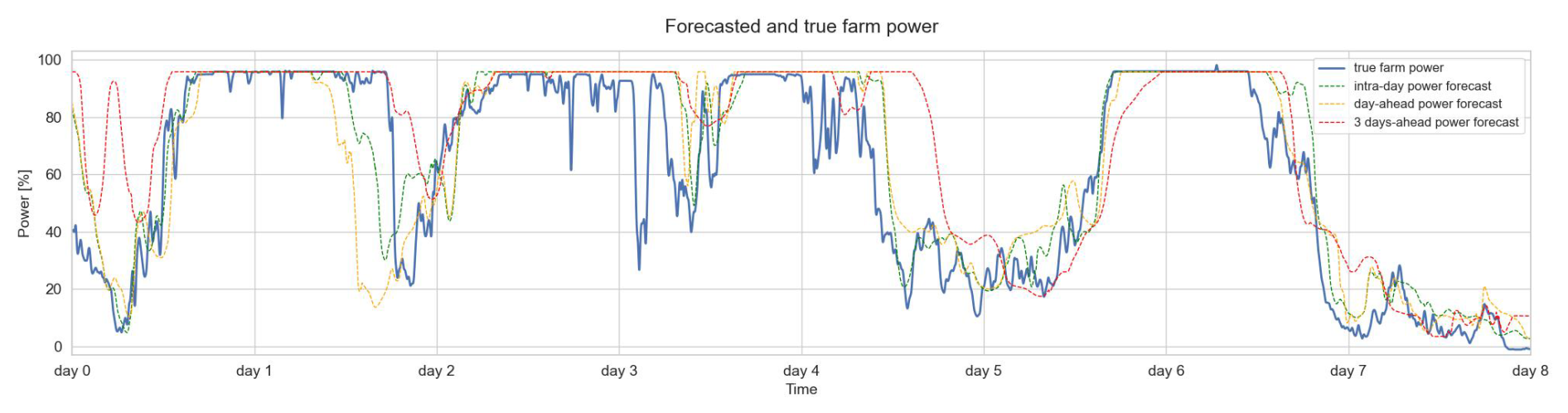
Figure 32Power forecasts for Wind Farm 1 based on wind forecasts with different forecast horizons for a time sequence of 8 d.
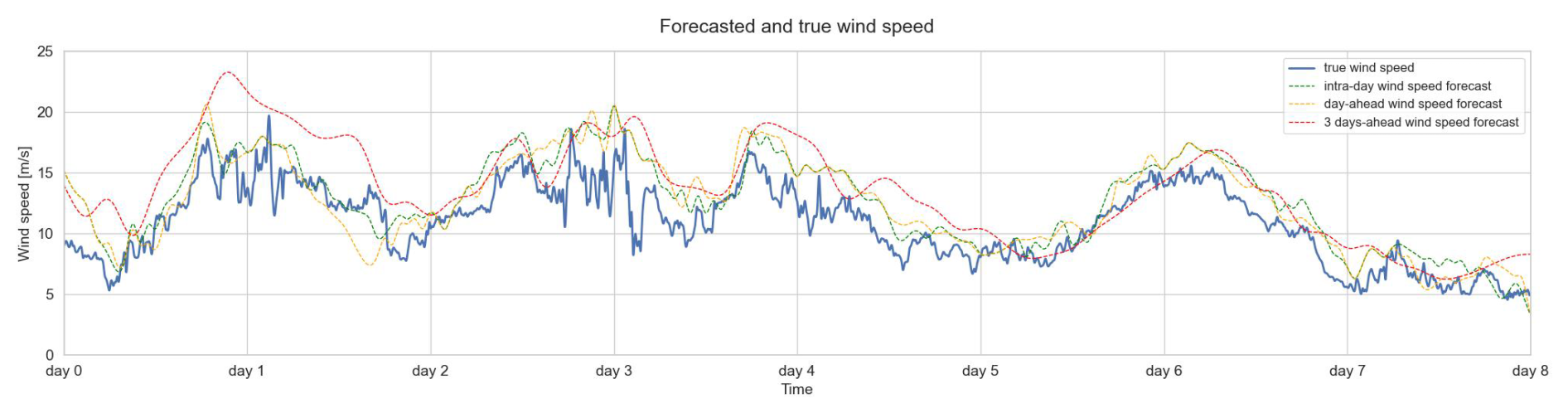
Figure 33Wind speed forecasts with different forecast horizons (from a third-party weather forecast provider).
The weather forecasts of different providers may differ between each other as they can be based on different weather models and data. Furthermore, they typically do not (accurately) take local effects into account, like for example neighbouring wind farms. These may cause a reduction in the wind speed, an increase in the wind turbulence intensity and a redirection of the wind due to wind blockage. Also coastal effects may have a significant impact on the wind speed and direction.
Figure 30 shows the correction factor being applied to the wind speed forecasts of a specific weather forecast provider for Wind Farm 1, depending on the forecast wind speed and direction. This correction factor has been calculated by mapping historical wind speed forecasts (those with the shortest lead time) from that weather forecast provider to the corresponding measured inflow wind speed of that farm. As can be seen in the figure, for wind directions between north-northwest and north-northeast, the wind speeds predicted by the correction model are only about 80 % of the forecast wind speeds. The reason is that in that upstream direction many wind farms are located within the immediate proximity. For wind speeds below 5 m s−1, the correction factor is higher than 1. This is due to the fact that the wind measurements on the turbines are not well calibrated and are overestimating these low wind speeds. For such wind speeds below the cut-in wind speed, turbines are shut off anyway.
In Fig. 31, it can be seen that for forecast wind directions in the sector from northwest, over south to east, the wind directions are in reality about 10 to 20° higher, meaning that airflows coming from these directions are deflected by about 10 to 20° in the clockwise direction (compared to the values forecasted by the weather forecast provider). In contrast, airflow coming from the sector east to northwest are deflected in the anti-clockwise direction. This corresponds to the fact that Wind Farm 1 is located in the south of the wind farm cluster and the cluster has a rectangular-like shape with the long axis in northwest–southeast direction. Due to blockage of the wind by the wind farm cluster, the airflow deviates through pressure build-up in front of the cluster slightly in the direction of the outside corners of the cluster, where it can flow next to the cluster. For lower wind speeds, thus with lower momentum, this deflection appears to be sharper than for higher wind speeds.
In addition, in Fig. 30 it can be seen that on average the corrected inflow wind speeds are lower than the ones forecasted by the weather service provider, also for wind directions without upstream wind farms causing wake. This may be may be attributable partly to coastal effects (the coast is the nearest in the east to south directions) and partly to the blockage effect of the wind farm cluster. For the wind directions in the south-southwest sector (directed towards the corner of the wind farm cluster) slightly increased wind speeds can be observed (especially for wind speeds between 11 and 12 m s−1). This might be an indication of the acceleration of the airflow at the corner of the cluster occurring jointly with the deflection due to the blockage effect. However, this may also be attributable to other reasons, such as underestimation by the weather forecast provider of wind speeds parallel to the coastline through the narrow Strait of Dover, as weather forecast models cannot model all local effects. For forecasts from another weather forecast provider and for historical ERA5 data, similar discrepancies in wind speed and wind directions are observed, however with different biases and/or variances.
Using the complete chain of models as shown in Fig. 2, starting with the models correcting the wind speed and direction forecasts, then the auxiliary models predicting the wind turbulence and air density, and finally the farm power model, the farm power can be forecasted for multiple time horizons. Figure 32 shows the 3 d ahead, day-ahead and intra-day power forecasts for an 8 d sequence for Wind Farm 1. Figure 33 shows the corresponding wind speed forecasts used as inputs for the power forecasts. As weather forecasts with a shorter lead time are usually more accurate than those with longer lead times, the resulting power forecasts become more accurate for shorter lead times as well.
This can be seen in Figs. 34 and 35, which show multiple error metrics for wind speed and direction forecasts with three different forecast horizons: intra-day (ID), day-ahead (DA) and 3 d ahead (3DA). From the bar charts it can be seen that the mean error (ME), mean average error (MAE) and root mean square error (RMSE) are higher for longer forecast horizons, whereas the R2 score decreases. It can also be seen that all error metrics for the wind speed forecasts improve significantly after application of the wind speed forecast correction model. Notice also that the mean error in the uncorrected wind speed forecasts is always larger than 0 m s−1. This is probably mainly due to the fact that the speed forecasts ignore the wind speed reduction caused by the wake of the upstream wind farms. After applying the correction model to the wind speed forecasts, the mean error is decreased to around 0 m s−1.
In Fig. 36, the error metrics of the corresponding wind farm power forecasts are shown. For each forecast, the same wind farm power model was used. For the orange bars, the uncorrected wind speed and direction forecasts were used, whereas for the green bars, first the wind speed and direction correction models were applied. The blue bars indicate the error metrics for the power predictions of the wind farm power model based on the actual wind inflow measurements (see Table 5, test data set of Wind Farm 1). It can be seen that the application of the wind correction models improves the farm power forecasts significantly. Note also that without the weather forecast correction models, the average wind farm power is greatly overestimated. This is not the case anymore after application of the weather forecast correction models. In addition, in the case of day-ahead forecasting, the MAE and RMSE are both reduced by about 30 %. For 3 d ahead forecasting, the relative improvements are smaller but still significant.
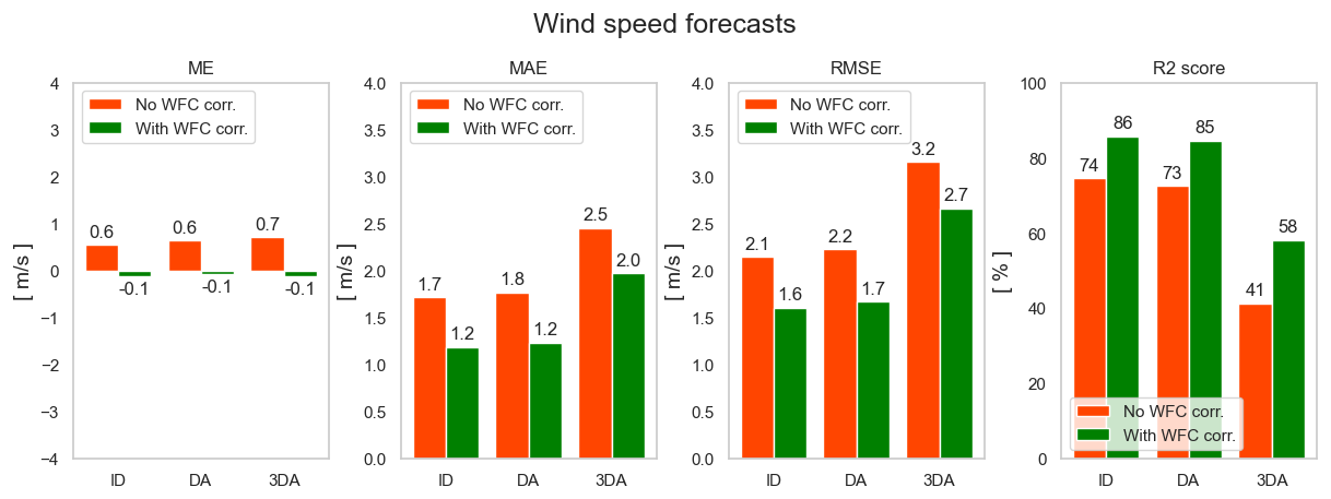
Figure 34Error metrics for intra-day (ID), day-ahead (DA) and 3 d ahead (3DA) wind speed forecasts for Wind Farm 1. The orange bars are the metrics for the wind speed forecasts of a commercial weather forecast provider. The green bars are the metrics after application of the weather forecast correction (WFC) model.
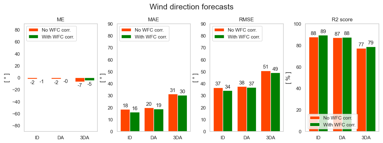
Figure 35Error metrics for intra-day (ID), day-ahead (DA) and 3 d ahead (3DA) wind direction forecasts for Wind Farm 1. The orange bars are the metrics for the wind direction forecasts of a commercial weather forecast provider. The green bars are the metrics after application of the weather forecast correction (WFC) model.
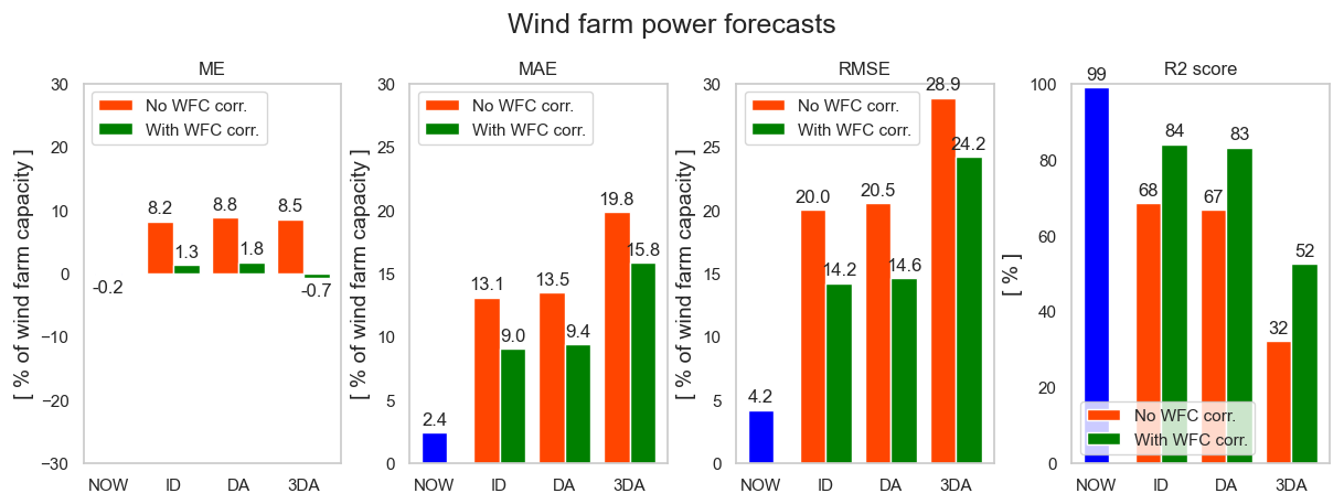
Figure 36Error metrics for intra-day (ID), day-ahead (DA) and 3 d ahead (3DA) wind farm power forecasts for Wind Farm 1. The orange bars are the metrics for the wind farm power forecasts based directly on the wind speed and direction forecasts of a commercial weather forecast provider. The green bars are the metrics for the wind farm power forecasts based on the corrected wind speed and direction forecasts. The blue bars show the corresponding error metrics for the wind farm model predictions based on actual (NOW) wind inflow measurements.
Note that a wind speed error of only 1 m s−1 represents about 12.5 % of the range between the cut-in and rated wind speed of a turbine (∼ 4 to ∼ 12 m s−1). Consequently, a wind speed forecasting error of that magnitude can result in a large farm power forecasting error, larger than the inaccuracy inherent to the farm power model itself. The relatively large errors in the weather forecasts should be no surprise, as the weather forecasts used in this example have a time resolution of only a 1 h (to be compared to the 1 min resolution of the used SCADA data and wind farm power model). Moreover, day-ahead forecasts have a forecasting lead time of up to 37 h (from the previous day at 11:00 to 24:00 of the next day). In addition, the processing time for making these weather forecasts may take up to 6 h so that the day-ahead forecasts may be based on data from 43 h ahead. The intra-day forecasts used in this example can have a lead time of up to half a day because the weather forecast data available for this work are updated only twice per day. Using more accurate weather forecasts updated more frequently and with a shorter time resolution will result in better farm power forecasts. One could argue that for the specific application of long-term wind farm power forecasting, using an accurate wind farm power prediction model with such a short time resolution (1 min) adds little value. It should be noted, however, that if for example a 1 h time resolution would be used for the training of the wind farm power model, the behaviour of the wind farm power controller and the temporal dynamics of inflow wind transients would not be captured by the farm power model, which are, however, crucial for other targeted applications of the model.
3.4 Computing hardware and software
All computing performed for this work, including the training of the ML models, was performed with a standard notebook (11th Gen Intel® Core™ i7-1165G7 processor at 2.80GHz, 16.0 GB of internal RAM, 64-bit operating system). All code is written in Python, with TensorFlow as the machine learning platform. Both are free, open-source software. This shows that the proposed model, in contrast to computationally intensive models, could be run on hardware that is readily accessible to wind farm operators.
In the present work, a novel methodology is proposed to forecast the power production of a wind farm. The methodology is based on a multi-component pipeline with a deep learning wind farm power model and a distinct machine learning model for integrating weather forecasts as its two main components.
The proposed wind farm power model relies solely on SCADA data from the wind farm itself, which are usually available to any wind farm operator. It captures the influence of several weather parameters, including wind speed, wind direction, turbulence intensity, wind direction variance and air density. Additionally, it captures the temporal dynamics of the wind inflow as well as the behaviour of the farm power controller. Also the number of turbines that are at standstill is taken into account. Notably, the model not only predicts the farm power with a high accuracy but also generates confidence intervals for these power predictions. Furthermore, the farm power model is capable of predicting the farm power in only a few milliseconds on PC, making it significantly faster than even low-fidelity physics-based models.
A separate deep learning model is employed to post-process the wind speed and direction forecasts from weather forecast providers. In doing so, it takes farm-external factors into account, such as wake generation by neighbouring wind farms, wind farm blockage, coastal effects and possible systematic forecasting errors from the respective weather forecast providers.
The two models, i.e. the wind farm power model and the model for post-processing weather forecasts, are independent of each other, which is a major advantage, as these can be trained and maintained separately.
Furthermore, in conjunction with a data-driven turbine power model, the farm wake losses can also be predicted.
The proposed methodology has been applied to two large real-world offshore wind farms. Performance metrics affirm a significantly improved prediction accuracy compared to some baseline machine learning models. In addition, validation sequences demonstrate the reliability of the predicted confidence intervals. Sensitivity analyses, performed on each of the model's input features, yield interpretable and physically meaningful results. In addition, the prediction capability of the farm power model is demonstrated for fluctuating inflow wind speeds.
It is also shown that the application of the post-processing model to the weather forecasts significantly improves the accuracy of the look-ahead wind farm power forecasts. Nevertheless, the accuracy for long forecast horizons remains predominantly limited by the limited accuracy of the third-party weather forecasts and not by the uncertainty inherent to the farm power model itself.
In further research, we will integrate the wind farm power prediction models as digital twins into applications where their high prediction speed and the simulation of the farm power controller are crucial.
In Table A1, the hyper-parameters of the wind farm power model (Sect. 2.3.1) are listed. Note that the hyper-parameters for the two wind farms are identical, except for the number of input features, as Wind Farm 2 has as additional input feature: “active-power capability of the farm” (Sect. 2.1.2).
In Table A2, the hyper-parameters of the wind speed and direction forecast mapping models (Sect. 2.3.3) are listed. Note that for the two models, the same hyper-parameters are used.
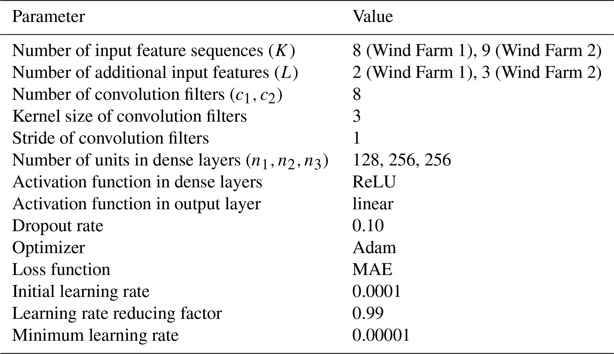
Table A2Hyper-parameters of the weather forecast mapping models.
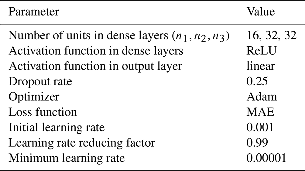
For those who are interested in the Python implementation of the methodology, please reach out to the corresponding author.
The SCADA data used within this work are not openly available due to confidentiality constraints.
SA: conceptualization, data curation, formal analysis, investigation, methodology, software, validation, visualization and writing (original draft preparation, review and editing). TV and PJD: supervision and paper review. AN: funding acquisition. JH: funding acquisition, supervision and paper review.
The contact author has declared that none of the authors has any competing interests.
Publisher’s note: Copernicus Publications remains neutral with regard to jurisdictional claims made in the text, published maps, institutional affiliations, or any other geographical representation in this paper. While Copernicus Publications makes every effort to include appropriate place names, the final responsibility lies with the authors.
This research was supported by the Flemish government (Flanders AI Research Program) and financially supported by the Energy Transition Fund projects Poseidon and Beforecast.
This paper was edited by Paul Fleming and reviewed by three anonymous referees.
Barthelmie, R. J., Hansen, K., Frandsen, S. T., Rathmann, O., Schepers, J., Schlez, W., Phillips, J., Rados, K., Zervos, A., Politis, E., and Chaviaropoulos, P. K.: Modelling and measuring flow and wind turbine wakes in large wind farms offshore, Wind Energy, 12, 431–444, 2009. a, b
Becker, M., Allaerts, D., and van Wingerden, J. W.: FLORIDyn – A dynamic and flexible framework for real-time wind farm control, J. Phys. Conf. Ser., 2265, 032103, https://doi.org/10.1088/1742-6596/2265/3/032103, 2022. a
Bleeg, J., Purcell, M., Ruisi, R., and Traiger, E.: Wind farm blockage and the consequences of neglecting its impact on energy production, Energies, 11, 1609, https://doi.org/10.3390/en11061609, 2018. a
Boersma, S., Doekemeijer, B. M., Gebraad, P. M., Fleming, P. A., Annoni, J., Scholbrock, A. K., Frederik, J. A., and van Wingerden, J.-W.: A tutorial on control-oriented modeling and control of wind farms, in: 2017 American control conference (ACC), Seattle, WA, USA, 24–26 May 2017, IEEE, 1–18, https://doi.org/10.23919/ACC.2017.7962923, 2017. a, b
Bossanyi, E. and Ruisi, R.: Axial induction controller field test at Sedini wind farm, Wind Energ. Sci., 6, 389–408, https://doi.org/10.5194/wes-6-389-2021, 2021. a
Braun, M., Gruhl, C., Hans, C. A., Härtel, P., Scholz, C., Sick, B., Siefert, M., Steinke, F., Stursberg, O., and von Berg, S. W.: Predictions and Decision Making for Resilient Intelligent Sustainable Energy Systems, arXiv [preprint], https://doi.org/10.48550/arXiv.2407.03021, 2024. a
Daenens, S., Vervlimmeren, I., Verstraeten, T., Daems, P.-J., Nowé, A., and Helsen, J.: Power prediction using high-resolution SCADA data with a farm-wide deep neural network approach, J. Phys. Conf. Ser., 2767, 092014, https://doi.org/10.1088/1742-6596/2767/9/092014, 2024. a
Fleming, P., King, J., Simley, E., Roadman, J., Scholbrock, A., Murphy, P., Lundquist, J. K., Moriarty, P., Fleming, K., van Dam, J., Bay, C., Mudafort, R., Jager, D., Skopek, J., Scott, M., Ryan, B., Guernsey, C., and Brake, D.: Continued results from a field campaign of wake steering applied at a commercial wind farm – Part 2, Wind Energ. Sci., 5, 945–958, https://doi.org/10.5194/wes-5-945-2020, 2020. a
Fleming, P. A., Ning, A., Gebraad, P. M., and Dykes, K.: Wind plant system engineering through optimization of layout and yaw control, Wind Energy, 19, 329–344, 2016. a
Foloppe, B., Munters, W., Buckingham, S., Vandevelde, L., and van Beeck, J.: Coupling of a dynamic wake model with WRF: a case study of the Belgian wind farms, in: 18th EAWE PhD Seminar, Bruges, Belgium,, 2 to 4 November 2022, 30–31, 2022. a
Gal, Y. and Ghahramani, Z.: Dropout as a Bayesian Approximation: Representing Model Uncertainty in Deep Learning, in: Proceedings of The 33rd International Conference on Machine Learning, edited by: Balcan, M. F. and Weinberger, K. Q., vol. 48 of Proceedings of Machine Learning Research, PMLR, New York, New York, USA, 1050–1059, https://proceedings.mlr.press/v48/gal16.html (last access: 25 July 2024), 2016. a
Gebraad, P. M. and Van Wingerden, J.: A control-oriented dynamic model for wakes in wind plants, J. Phys. Conf. Ser., 524, 012186, https://doi.org/10.1088/1742-6596/524/1/012186, 2014. a
IEA: Renewables 2022 – Analysis and forecast to 2027, https://iea.blob.core.windows.net/assets/ada7af90-e280-46c4-a577-df2e4fb44254/Renewables2022.pdf (last access: 25 July 2024), 2022. a
Jensen, N. O.: A note on wind generator interaction, vol. 2411, Citeseer, https://backend.orbit.dtu.dk/ws/portalfiles/portal/55857682/ris_m_2411.pdf (last access: 25 July 2024), 1983. a
Kisvari, A., Lin, Z., and Liu, X.: Wind power forecasting–A data-driven method along with gated recurrent neural network, Renewable Energy, 163, 1895–1909, 2021. a, b
Kölle, K., Göçmen, T., Garcia-Rosa, P. B., Petrović, V., Eguinoa, I., Vrana, T. K., Long, Q., Pettas, V., Anand, A., Barlas, T. K., Cutululis, N., Manjock, A., Tande, J. O., Ruisi, R., and Bossanyi, E.: Towards integrated wind farm control: Interfacing farm flow and power plant controls, Advanced Control for Applications: Engineering and Industrial Systems, 4, e105, https://doi.org/10.1002/adc2.105, 2022. a
Larsen, G. C., Madsen, H. A., Bingöl, F., Mann, J., Ott, S., Sorensen, J. N., Okulov, V., Troldborg, N., Nielsen, M., Thomsen, K., Larsen, T. J., and Mikkelsen, R.: Dynamic wake meandering modeling, ISBN 978-87-550-3602-4, https://www.osti.gov/etdeweb/servlets/purl/20941220#page=1.00&gsr=0 (last access: 25 July 2024), 2007. a
Laves, M.-H., Ihler, S., Fast, J. F., Kahrs, L. A., and Ortmaier, T.: Well-calibrated regression uncertainty in medical imaging with deep learning, in: Medical Imaging with Deep Learning, PMLR, 393–412, https://proceedings.mlr.press/v121/laves20a/laves20a.pdf (last access: 25 July 2024), 2020. a
LeCun, Y., Bengio, Y., and Hinton, G.: Deep learning, Nature, 521, 436–444, 2015. a
Lee, J. C. Y. and Fields, M. J.: An overview of wind-energy-production prediction bias, losses, and uncertainties, Wind Energ. Sci., 6, 311–365, https://doi.org/10.5194/wes-6-311-2021, 2021. a
Lin, Z. and Liu, X.: Wind power forecasting of an offshore wind turbine based on high-frequency SCADA data and deep learning neural network, Energy, 201, 117693, https://doi.org/10.1016/j.energy.2020.117693, 2020. a
Liu, T., Huang, Z., Tian, L., Zhu, Y., Wang, H., and Feng, S.: Enhancing wind turbine power forecast via convolutional neural network, Electronics, 10, 261, https://doi.org/10.3390/electronics10030261, 2021. a
Martínez-Tossas, L. A., Annoni, J., Fleming, P. A., and Churchfield, M. J.: The aerodynamics of the curled wake: a simplified model in view of flow control, Wind Energ. Sci., 4, 127–138, https://doi.org/10.5194/wes-4-127-2019, 2019. a
Martínez-Tossas, L. A., King, J., Quon, E., Bay, C. J., Mudafort, R., Hamilton, N., Howland, M. F., and Fleming, P. A.: The curled wake model: a three-dimensional and extremely fast steady-state wake solver for wind plant flows, Wind Energ. Sci., 6, 555–570, https://doi.org/10.5194/wes-6-555-2021, 2021. a
Meyers, J., Bottasso, C., Dykes, K., Fleming, P., Gebraad, P., Giebel, G., Göçmen, T., and van Wingerden, J.-W.: Wind farm flow control: prospects and challenges, Wind Energ. Sci., 7, 2271–2306, https://doi.org/10.5194/wes-7-2271-2022, 2022. a
Nejad, A. R., Keller, J., Guo, Y., Sheng, S., Polinder, H., Watson, S., Dong, J., Qin, Z., Ebrahimi, A., Schelenz, R., Gutiérrez Guzmán, F., Cornel, D., Golafshan, R., Jacobs, G., Blockmans, B., Bosmans, J., Pluymers, B., Carroll, J., Koukoura, S., Hart, E., McDonald, A., Natarajan, A., Torsvik, J., Moghadam, F. K., Daems, P.-J., Verstraeten, T., Peeters, C., and Helsen, J.: Wind turbine drivetrains: state-of-the-art technologies and future development trends, Wind Energ. Sci., 7, 387–411, https://doi.org/10.5194/wes-7-387-2022, 2022. a
NREL: OpenFAST, https://github.com/OpenFAST/openfast, GitHub [code], https://github.com/OpenFAST/openfast (last access: 25 July 2024), 2025a. a
NREL: FLORIS Wake Modeling and Wind Farm Controls Software (FLORIS v3.4.1), GitHub [code], https://github.com/NREL/floris (last access: 25 July 2024), 2025b. a
NREL: Simulator fOr Wind Farm Applications (SOWFA), https://github.com/NREL/SOWFA, GitHub [code], https://github.com/NREL/SOWFA (last access: 25 July 2024), 2025c. a
Nygaard, N. G., Steen, S. T., Poulsen, L., and Pedersen, J. G.: Modelling cluster wakes and wind farm blockage, J. Phys. Conf. Ser., 1618, 062072, https://doi.org/10.1088/1742-6596/1618/6/062072, 2020. a
Park, J. and Park, J.: Physics-induced graph neural network: An application to wind-farm power estimation, Energy, 187, 115883, https://doi.org/10.1016/j.energy.2019.115883, 2019. a
Perez-Sanjines, F., Verstraeten, T., Nowé, A., and Helsen, J.: Deep ensemble with Neural Networks to model power curve uncertainty, J. Phys. Conf. Ser., 2362, 012029, https://doi.org/10.1088/1742-6596/2362/1/012029, 2022. a, b
Pettas, V., Kretschmer, M., Clifton, A., and Cheng, P. W.: On the effects of inter-farm interactions at the offshore wind farm Alpha Ventus, Wind Energ. Sci., 6, 1455–1472, https://doi.org/10.5194/wes-6-1455-2021, 2021. a
Piotrowski, P., Rutyna, I., Baczyński, D., and Kopyt, M.: Evaluation metrics for wind power forecasts: A comprehensive review and statistical analysis of errors, Energies, 15, 9657, https://doi.org/10.3390/en15249657, 2022. a
Pombo, D. V., Göçmen, T., Das, K., and Sørensen, P.: Multi-horizon data-driven wind power forecast: From nowcast to 2 days-ahead, in: 2021 International Conference on Smart Energy Systems and Technologies (SEST), 1–6, https://doi.org/10.1109/SEST50973.2021.9543173, 2021. a
Porté-Agel, F., Bastankhah, M., and Shamsoddin, S.: Wind-turbine and wind-farm flows: A review, Boundary-Lay. Meteorol., 174, 1–59, https://doi.org/10.1007/s10546-019-00473-0, 2020. a, b
Sanderse, B., Van der Pijl, S., and Koren, B.: Review of computational fluid dynamics for wind turbine wake aerodynamics, Wind Energy, 14, 799–819, 2011. a, b
Schepers, J.: WakeFarm: nabij zog model en ongestoord wind snelheidsveld, Energieonderzoek Centrum Nederland, Technical Report, ECN-C-98-016, 1998. a
Sood, I., Simon, E., Vitsas, A., Blockmans, B., Larsen, G. C., and Meyers, J.: Comparison of large eddy simulations against measurements from the Lillgrund offshore wind farm, Wind Energ. Sci., 7, 2469–2489, https://doi.org/10.5194/wes-7-2469-2022, 2022. a
Strickland, J. M., Gadde, S. N., and Stevens, R. J.: Wind farm blockage in a stable atmospheric boundary layer, Renewable Energy, 197, 50–58, https://doi.org/10.1016/j.renene.2022.07.108, 2022. a
Ti, Z., Deng, X. W., and Zhang, M.: Artificial Neural Networks based wake model for power prediction of wind farm, Renewable Energy, 172, 618–631, 2021. a, b
University of Hannover: Parallelized Large-Eddy Simulation Model (PALM), GitLab [code], https://gitlab.palm-model.org/releases/palm_model_system (last access: 25 July 2024), 2021. a
Van Der Laan, M., Pena, A., Volker, P., Hansen, K. S., Sørensen, N. N., Ott, S., and Hasager, C. B.: Challenges in simulating coastal effects on an offshore wind farm, J. Phys. Conf. Ser., 854, 012046, https://doi.org/10.1088/1742-6596/854/1/012046, 2017. a
Verstraeten, T., Nowé, A., Keller, J., Guo, Y., Sheng, S., and Helsen, J.: Fleetwide data-enabled reliability improvement of wind turbines, Renew. Sust. Energ. Rev., 109, 428–437, 2019. a
Verstraeten, T., Daems, P.-J., Bargiacchi, E., Roijers, D. M., Libin, P. J., and Helsen, J.: Scalable optimization for wind farm control using coordination graphs, arXiv [preprint], https://doi.org/10.48550/arXiv.2101.07844, 2021. a
Wang, H.-Z., Li, G.-Q., Wang, G.-B., Peng, J.-C., Jiang, H., and Liu, Y.-T.: Deep learning based ensemble approach for probabilistic wind power forecasting, Appl. Energ., 188, 56–70, 2017. a
Wang, Y., Zou, R., Liu, F., Zhang, L., and Liu, Q.: A review of wind speed and wind power forecasting with deep neural networks, Appl. Energ., 304, 117766, https://doi.org/10.1016/j.apenergy.2021.117766, 2021. a
Yin, X. and Zhao, X.: Big data driven multi-objective predictions for offshore wind farm based on machine learning algorithms, Energy, 186, 115704, https://doi.org/10.1016/j.energy.2019.07.034, 2019. a
Zehtabiyan-Rezaie, N., Iosifidis, A., and Abkar, M.: Physics-guided machine learning for wind-farm power prediction: Toward interpretability and generalizability, PRX Energy, 2, 013009, https://doi.org/10.1103/PRXEnergy.2.013009, 2023. a, b