Bayesian uncertainty quantification of engineering models for wind farm–atmosphere interaction

Accurate modeling of wind farm–atmosphere interactions is critical for reliable energy yield assessments and flow control strategies. However, formal model comparison methodologies that quantify model form uncertainty by also accounting for parameter uncertainty are still lacking. This study presents an enhanced Bayesian uncertainty quantification framework for the calibration and validation of engineering wind farm flow models. Building on previous work, the framework explicitly incorporates model inadequacy through a parametrized model error distribution, enabling the separation of model and measurement uncertainties. The improved framework is demonstrated using a large-eddy simulation dataset for wind farm blockage and atmospheric gravity waves in conventionally neutral boundary layers. Two models of differing fidelity – a standard Gaussian wake model and an atmospheric perturbation model (APM) – are calibrated and compared. The posterior distribution of the model parameters reveals insights into model behavior and highlights areas for further improvement, for instance, when estimated parameter values are inconsistent across the model chain. In addition, it is shown that not explicitly incorporating model inadequacy results in an overly confident posterior distribution and renders derived stochastic flow models incapable of representing model uncertainty. A comparison of the quantified model uncertainty shows that the APM has significantly lower uncertainty than a standard wake model for this dataset, as the wake model is unable to represent wind farm blockage effects. This demonstrates the utility of the framework for objective model comparison with quantified parameter and model uncertainty given a reference dataset. Both the framework and the parallelized sequential Monte Carlo algorithm for accelerated posterior sampling are made available through the open-source Python package UMBRA.

1 Introduction

Wind farm flow model bias and uncertainty directly impact both the profitability of wind projects through pre-construction energy yield assessments (Lee and Fields, 2021) and the financial targets of wind developers through production forecasts (Ørsted, 2019). Although the estimation bias in annual energy predictions (AEPs) has steadily declined in the last 2 decades, the uncertainty remained of similar magnitude (Lee and Fields, 2021). Historically, wind farm performance is one of the largest contributors to AEP uncertainty, in part due to the uncertainty of the power losses on downstream turbines due to turbine wake effects (Clifton et al., 2016; Lee and Fields, 2021). Although models for these wake losses can reproduce trends in benchmark observations, their precision is highly variable, motivating the use of more precise and delineated observations of wind farms under many different operating and atmospheric conditions instead of those averaged over long periods of time (Moriarty et al., 2014). Moreover, the increasing capacity density and size of wind turbines require new wind farm flow models that consider the atmospheric boundary layer from the surface to the free atmosphere to model effects such as wind farm blockage (Allaerts and Meyers, 2019) and wakes (Bastankhah et al., 2024). To turn new wind farm flow models into reliable and cost-effective tools, objective methods are needed to validate them, quantify their uncertainty, and eventually calibrate them with a wide variety of flow conditions (Rodrigo et al., 2017). The present article studies the use of Bayesian uncertainty quantification (UQ) as an objective method for model comparison given a reference dataset and calibration with quantified parameter uncertainty.

Many small- to large-scale benchmarking studies have validated the suitability of wind turbine wake models to represent energy losses in downstream turbines with historical power data (see Doekemeijer et al., 2022, for a comprehensive overview). Typically, these studies compare metrics such as farm power, turbine power for a given bin of wind directions, and wake loss while using default wake model parameters (Doekemeijer et al., 2022). This is common practice, as it is the most objective way of quantifying the baseline performance of the models (Rodrigo et al., 2017). However, it is known that the wake model bias is site-specific (Nygaard, 2015) and that the wake recovery differs between offshore and onshore wind farms (Barthelmie et al., 2009; Göçmen et al., 2016) and with atmospheric conditions (Abkar and Porté-Agel, 2015; Niayifar and Porté-Agel, 2016; Klemmer and Howland, 2025). Therefore, site-specific model tuning is crucial for accurate production forecasts. Moreover, in wind farm flow control, the flow model may be tuned to site-specific data in an open- or closed-loop fashion to adequately represent the flow field at any time (Göçmen et al., 2022; Meyers et al., 2022). Therefore, any model validation procedure may benefit from including model calibration so that model performance in practical applications can be compared objectively.

Concerning the quantification of uncertainty, one must distinguish between forward (data-free) and inverse (data-driven) UQ methods (Xiao and Cinnella, 2019). Forward UQ examines the effect of prespecified uncertainties on model inputs on the model outcome and is widely used to quantify the effect of wind resource variability on AEP estimates (Lackner et al., 2007; Kwon, 2010; Clerc et al., 2012). The procedure of Gaumond et al. (2014) to assess the effect of wind direction uncertainty on the predicted power of wake models also adheres to this approach. Despite being rigorous, forward UQ relies on the estimates of the constituent uncertainties, which may be subjective (Nygaard, 2015). Inverse UQ estimates the uncertainty of the model, and possibly its parameters, by comparing it with measured data. The estimated distribution of the discrepancy between model predictions and measurements determines the model uncertainty through its width and the model bias through its mean. With an inverse UQ using operational data from 19 offshore wind farms, Nygaard et al. (2022) showed that the uncertainty on the predicted wake loss relative to the observed wake loss is less than 10 % of the observed loss for the TurboPark model. This is significantly lower than previously estimated (Walker et al., 2015), in part due to thorough data processing and the inclusion of heterogeneous background flow. However, the uncertainty of the model is still overestimated because it is not separated from the experimental uncertainty. With Bayesian inverse UQ, it is possible to separate the measurement and model uncertainty, as demonstrated with operational power data from the Westermost Rough wind farm, while also accounting for the uncertainty of the model parameters (Aerts et al., 2023).

In Bayesian UQ, the model parameters and sources of uncertainties are characterized by probability distributions, which represent our knowledge about them and which can be updated when more data become available. Compared to deterministic model calibration methods (see van Binsbergen et al., 2024, for a comprehensive overview), Bayesian calibration gives not only the “best” parameters, but a joint posterior distribution with information on the parameter uncertainties and their correlations given the dataset (Aerts et al., 2023). The posterior parameter distribution may inform modelers about missing physics, when parameter values are estimated differently throughout the model chain. For example, LoCascio et al. (2023) showed that the posterior mean wake expansion rate and its uncertainty differ for different wake-merging methods, which is a cautionary finding for a modular approach to wake modeling. In addition, Zhang and Zhao (2020) and LoCascio et al. (2023) have proposed using the posterior distribution of the model parameters to obtain stochastic wake models, which can be used in wake steering under uncertainty (Howland, 2021). However, the current approaches to obtain such stochastic models include only the epistemic uncertainty (i.e., due to limited data) on the model parameters and not the model uncertainty due to varying physical phenomena not captured by the (deterministic) model.

In this study, we improve on a previously developed Bayesian UQ framework (Aerts et al., 2023) and demonstrate its use in a controlled environment with large model uncertainty. To this end, we select a large-eddy simulation dataset for blockage due to atmospheric gravity waves (Lanzilao and Meyers, 2024) as reference data and perform an inverse UQ for a standard wake model and a recently developed atmospheric perturbation model (Devesse et al., 2024b). Specifically, we present how the model uncertainty can be incorporated into the Bayesian framework to obtain stochastic models that include model uncertainty. In addition, we illustrate how the adequate inclusion of model uncertainty is crucial to obtain a correct posterior distribution of the empirical parameters, which is used in the current stochastic wake models. Lastly, we show how the Bayesian UQ framework can be used for objective model comparison with quantified model and parameter uncertainty. In contrast to previous studies (Zhang and Zhao, 2020; Aerts et al., 2023; LoCascio et al., 2023), which relied on inherently serial Markov chain Monte Carlo (MCMC) algorithms such as (Adaptive) Metropolis Hastings (Haario et al., 2001) and Hamiltonian Monte Carlo with No-U-Turn tuning (Hoffman and Gelman, 2014) to approximate the posterior distribution, we employ an inherently parallel sampling algorithm that still performs so-called “exact” posterior inference. The parallelized sampler and Bayesian framework are made available in an open-source Python package coined UMBRA: Uncertainty Modeling toolbox for Bayesian data Re-Analysis.

The improved Bayesian UQ framework is presented in Sect. 2, together with the inherently parallel algorithm to sample the posterior. The setup of the demonstration case is introduced in Sect. 3, by presenting the essential parts of the wind farm flow models and dataset. The results of the inverse UQ analyses are presented in Sect. 4, with emphasis on the framework's adequacy (Sect. 4.1), its application to objective model comparison with UQ (Sect. 4.2), and the generalizability of the findings (Sect. 4.3). A summary and outlook are given in Sect. 5.

2 Bayesian uncertainty quantification

We first discuss how different sources of uncertainty are included in the UQ framework in Sect. 2.1, building on earlier work (Aerts et al., 2023). Section 2.2 demonstrates how this formulation naturally leads to Bayesian updating from a prior to a posterior distribution and introduces the posterior predictive distribution as a key tool for validation in Bayesian UQ. Once the framework is introduced, we demonstrate the consequences of neglecting the model error in Sect. 2.3. The parallelizable algorithm employed for posterior sampling is detailed in Sect. 2.4.

2.1 Sources of uncertainty

Wind farm flow models aim to predict quantities of interest for a given atmospheric state. When focusing on turbine-level power output, the idealized “true process” T(ψ) would yield the power $\mathcal{P}\in {\mathbb{R}}^{N_{\mathrm{T}}}$ of the N_T turbines, normalized by the output of an undisturbed upstream turbine, given a complete description of the wind farm and atmospheric state in a general vector ψ:

$$\begin{array}{}\text{(1)}& {\displaystyle }{\displaystyle }\mathcal{P}=\mathit{T}\left(\mathit{\psi }\right).\end{array}$$

In practice, the true process is approximated by a model M(ϑ_e,φ), which relies on empirical parameters ϑ_e and a partial state description φ. This approximation introduces model bias and uncertainty, which we would like to represent and quantify (Sect. 2.1.1). Since the true process is only accessible through measurements, measurement uncertainty also arises (Sect. 2.1.2). Moreover, the most representative values of ϑ_e for the given conditions are initially unknown. Section 2.1.3 describes how our initial knowledge about the model parameters, bias, and uncertainty can be represented in a prior probability density. In what follows, we write a random variable and its realization with a calligraphic symbol 𝓣, its probability distribution as p(𝓣), and the function that uniquely determines it from other random variables as T(ψ) so that $p\left(\mathcal{T}\right|\mathit{\psi })=\mathit{\delta }(\mathcal{T}-\mathit{T}\left(\mathit{\psi }\right))$, with δ(⋅) the Dirac delta distribution.

2.1.1 Model error

Since the wind farm flow model is typically imperfect, we can define an additive model error E_B(ϑ_e,ψ) that depends on the choice of the model parameters ϑ_e and the state of the wind farm and atmosphere ψ:

$$\begin{array}{}\text{(2)}& {\displaystyle }{\displaystyle }\mathit{T}\left(\mathit{\psi }\right)\triangleq \mathit{M}({\mathit{\vartheta }}_{\mathrm{e}},\mathit{\phi })+{\mathit{E}}_B({\mathit{\vartheta }}_{\mathrm{e}},\mathit{\psi }).\end{array}$$

Note that the model error is, in fact, deterministic given ϑ_e and ψ, so that its distribution $p\left({\mathcal{E}}_B\right|{\mathit{\vartheta }}_{\mathrm{e}},\mathit{\psi })=\mathit{\delta }({\mathcal{E}}_B-{\mathit{E}}_B({\mathit{\vartheta }}_{\mathrm{e}},\mathit{\psi }))$. However, since usually only a subset φ of the variables $\mathit{\psi }=(\mathit{\phi },{\mathit{\psi }}^{\prime })$ describing the atmospheric conditions is available or included as input to the model, we are interested in the distribution of the true process 𝓣 conditioned on the observed conditions φ, given by

$$\begin{array}{}\text{(3a)}& {\displaystyle }p\left(\mathcal{T}\right|\mathit{\phi })=\int p(\mathcal{T}\left|\mathit{\psi }\right)p\left({\mathit{\psi }}^{\prime }\right|\mathit{\phi })\mathrm{d}{\mathit{\psi }}^{\prime }\text{(3b)}& {\displaystyle }=\int \mathit{\delta }\left(\mathit{M}\right({\mathit{\vartheta }}_{\mathrm{e}},\mathit{\phi })+{\mathit{E}}_B({\mathit{\vartheta }}_{\mathrm{e}},\mathit{\psi })-\mathcal{T})p\left({\mathit{\psi }}^{\prime }\right|\mathit{\phi })\mathrm{d}{\mathit{\psi }}^{\prime }.\end{array}$$

The unmodeled or unobserved variations in atmospheric conditions ψ^′ thus introduce uncertainty in the conditional process 𝓣|φ through their influence on the model error E_B(ϑ_e,ψ). However, if we allow the model parameters ϑ_e to depend on the unobserved conditions, the uncertainty on 𝓣|φ may also be reflected in a distribution of the model parameters ϑ_e. Hence, we have to choose whether to incorporate this uncertainty on the process 𝓣|φ, which we will further refer to as model uncertainty, within the model parameters ϑ_e or in the model error 𝓔_B, by fixing the other. Allowing both the model parameters and the model uncertainty to vary with the unknown conditions ψ^′ causes them to partially contribute in the same way to the total model uncertainty. Such similar contributions to the total model uncertainty are indistinguishable when quantifying the constituent uncertainties from data, rendering the inverse problem underdetermined.

The first option is to incorporate the model uncertainty within the model parameters through a hierarchical stochastic prior (see also Sargsyan et al., 2015; Wu et al., 2018a). To this end, we fix the model error ${\mathit{E}}_B({\mathit{\vartheta }}_{\mathrm{e}},\mathit{\psi })={\mathit{\mu }}_B$, so that this relation defines the dependence of the model parameters ϑ_e on the wind farm–atmosphere state ψ. Propagating the distribution of the unknown conditions $p\left({\mathit{\psi }}^{\prime }\right|\mathit{\phi })$ through this implicit relation yields a distribution of ϑ_e, which is unknown. If we are only interested in the first- and second-order moments, we can parametrize it as a normal distribution ${\mathit{\vartheta }}_{\mathrm{e}}\sim \mathcal{N}({\mathit{\mu }}_{\mathit{\vartheta }},{\mathit{\sigma }}_{\mathit{\vartheta }}^{\mathrm{2}})$ with mean μ_ϑ and variance ${\mathit{\sigma }}_{\mathit{\vartheta }}^{\mathrm{2}}$ for a scalar parameter ϑ_e∈ℝ, which is the maximum entropy distribution in that case (McElreath, 2018). A change in variables then gives

$$\begin{array}{}\text{(4a)}& {\displaystyle }p\left(\mathcal{T}\right|\mathit{\phi })=\int \mathit{\delta }(\mathit{M}({\mathit{\vartheta }}_{\mathrm{e}},\mathit{\phi })+{\mathit{\mu }}_B-\mathcal{T}\left)\mathcal{N}\right({\mathit{\vartheta }}_{\mathrm{e}};{\mathit{\mu }}_{\mathit{\vartheta }},{\mathit{\sigma }}_{\mathit{\vartheta }}^{\mathrm{2}})\mathrm{d}{\mathit{\vartheta }}_{\mathrm{e}}\text{(4b)}& {\displaystyle }\approx \mathcal{N}(\mathcal{T};\mathit{M}({\mathit{\mu }}_{\mathit{\vartheta }},\mathit{\phi })+{\mathit{\mu }}_B,{\mathit{\sigma }}_{\mathit{\vartheta }}^{\mathrm{2}}{\mathit{J}}_M{\mathit{J}}_M^{\top }),\end{array}$$

where the approximation corresponds to a linearization of the model $\mathit{M}({\mathit{\vartheta }}_{\mathrm{e}},\mathit{\phi })\approx \mathit{M}({\mathit{\mu }}_{\mathit{\vartheta }},\mathit{\phi })+{\mathit{J}}_M({\mathit{\vartheta }}_{\mathrm{e}}-{\mathit{\mu }}_{\mathit{\vartheta }})$ with the Jacobian ${\mathit{J}}_M\in {\mathbb{R}}^{N_{\mathrm{T}}}$. Hence, the model uncertainty is determined by the model parameter uncertainty σ_ϑ and the model structure through the Jacobian J_M. However, the model uncertainty may have a different structure than the model itself. Taking the example of a wake model with an unknown wake expansion rate, the model uncertainty on the upstream turbines due to blockage cannot be captured in this approach, as the sensitivity of the upstream turbine power to the wake expansion rate is zero. Hence, an additional model error term is generally needed. Moreover, a forward UQ is still necessary to translate the uncertainty on the model parameters to uncertainty on the model output, which is typically of interest for many practical applications.

The second approach attributes the model uncertainty only to the model error term. To that end, we fix the model parameter values ϑ_e and let the model error E_B(ϑ_e,ψ) vary with the unknown conditions. Hence, the model uncertainty is represented in the distribution of the model error $p\left({\mathcal{E}}_B\right|{\mathit{\vartheta }}_{\mathrm{e}},\mathit{\phi })$, which is no longer a Dirac delta if a part ψ^′ of the wind farm–atmosphere state $\mathit{\psi }=(\mathit{\phi },{\mathit{\psi }}^{\prime })$ is unknown. The distribution $p\left({\mathcal{E}}_B\right|{\mathit{\vartheta }}_{\mathrm{e}},\mathit{\phi })$ is a priori unknown, but if we are mainly interested in its first- and second-order moments, we can parametrize it as a multivariate normal distribution with expected value μ_B and covariance matrix Σ_B:

$$\begin{array}{ll}{\displaystyle }p\left({\mathcal{E}}_B\right|{\mathit{\vartheta }}_{\mathrm{e}},\mathit{\phi })& {\displaystyle }=\int p\left({\mathcal{E}}_B\right|{\mathit{\vartheta }}_{\mathrm{e}},\mathit{\psi }\left)p\right({\mathit{\psi }}^{\prime }\left|\mathit{\phi }\right)\mathrm{d}{\mathit{\psi }}^{\prime }\\ \text{(5)}& {\displaystyle }& {\displaystyle }\approx \mathcal{N}({\mathcal{E}}_B;{\mathit{\mu }}_B,{\mathbf{\Sigma }}_B).\end{array}$$

We will further approximate $p\left({\mathcal{E}}_B\right|{\mathit{\vartheta }}_{\mathrm{e}},\mathit{\phi })\approx p({\mathcal{E}}_B\left|\mathit{\phi }\right)$ (Kennedy and O'Hagan, 2001), but since the model error depends on the choice of model parameters, this requires including sufficient prior knowledge on the mean model error μ_B (Brynjarsdóttir and O'Hagan, 2014), as will be discussed in Sect. 2.1.3. This second approach yields a model error distribution that is independent of the model structure and is readily interpreted as uncertainty on either the model or the model error due to additivity. To allow a general model error uncertainty parametrization while avoiding the problem becoming underdetermined, we opt for the second approach.

The current parametrization of the model error distribution scales with the number of turbines N_T in the farm since the mean model error ${\mathit{\mu }}_B\in {\mathbb{R}}^{N_{\mathrm{T}}}$ and its covariance matrix ${\mathbf{\Sigma }}_B\in {\mathbb{R}}^{N_{\mathrm{T}}\times N_{\mathrm{T}}}$. To reduce its dimensionality, we follow the same approach as in our previous work (Aerts et al., 2023). The correlations in Σ_B are neglected, and the mean and standard deviation of the model error on the power of the turbine i are binned based on the number of upstream turbines ζ(i) that cause a wake loss on the turbine i greater than 1 % of the free stream wind speed. Hence,

$$\begin{array}{}\text{(6)}& {\displaystyle }& {\displaystyle }{\mathit{\mu }}_{B,i}={\mathit{\delta }}_{\mathit{\zeta }\left(i\right)}\text{(7)}& {\displaystyle }& {\displaystyle }{\mathrm{\Sigma }}_{B,ij}={\mathit{\delta }}_{ij}{\mathit{\sigma }}_{B,\mathit{\zeta }\left(i\right)}^{\mathrm{2}},\end{array}$$

where δ_ij is the Kronecker delta. As such, the model error distribution is parametrized by the parameters ${\mathit{\vartheta }}_b=\mathit{\{}{\mathit{\delta }}_{\mathit{\zeta }},{\mathit{\sigma }}_{B,\mathit{\zeta }}{\mathit{\}}}_{\mathit{\zeta }=\mathrm{0}}^{{\mathit{\zeta }}_{\text{max}}}$ with ζ=0 as the index for the upstream turbines, ζ=1 as the index for turbines with one upstream turbine that wakes them, and so forth.

2.1.2 Measurement error

The true process can only be observed with measurements $\stackrel{\mathrm{̃}}{\mathcal{P}}$, which come with a measurement error 𝓔_M:

$$\begin{array}{}\text{(8)}& {\displaystyle }{\displaystyle }\stackrel{\mathrm{̃}}{\mathcal{P}}=\mathcal{T}+{\mathcal{E}}_{\mathrm{M}}.\end{array}$$

We will make the simplifying assumption that the measurement error is independent of the unobserved or unmodeled physics ψ^′ such that ${\mathcal{E}}_{\mathrm{M}}|\mathit{\psi }\approx {\mathcal{E}}_{\mathrm{M}}|\mathit{\phi }$ (Aerts et al., 2023). Since most engineering wind farm flow models represent stationary atmospheric flows, their predictions should be compared with time-averaged data. However, observational and high-fidelity simulation data are typically subjected to temporally resolved turbulence. Because only a finite time period is available for averaging due to changing atmospheric conditions or computational constraints, the measurement error consists of both the error of the apparatus and the averaging error. The measurement bias and standard deviation due to the apparatus are typically known a priori, such that the distribution of the apparatus error can be taken as a normal distribution based on these quantities. In what follows, we will presume that the averaging error dominates. This is certainly true for simulation data, as is the case in this article. Due to the central limit theorem and given that the estimator is unbiased, the measurement error then follows a multivariate normal distribution with zero mean and a covariance matrix Σ_T.

The averaging error covariance matrix Σ_T on the mean can either be prespecified or unknown. For independent measurements for the same atmospheric condition, the uncertainty on the average of the measurements can be estimated as the sample variance divided by the number of measurements (Wasserman, 2004). Equivalently, all individual measurements can be used with the sample variance, given that they are independent and represent the same atmospheric state. For a correlated time series, the moving block bootstrap can be employed (Garcia et al., 2005). If no information is available, the averaging error covariance can also be estimated directly from the data based on a parametrization with parameters ϑ_t (Aerts et al., 2023). However, if the covariance structures between the averaging error and the model error are not sufficiently different, they are indistinguishable. Therefore, it is preferred to use the estimated uncertainty on the mean if available.

In practice, the inflow conditions can also be uncertain due to any kind of measurement error. This inflow uncertainty may be propagated through the model with a marginalization similar to that in Eq. (4). Note that this procedure is similar to that of Gaumond et al. (2014) to incorporate the effect of wind direction variability on the mean power but also includes the resulting variance of the model output. In that manner, a part of the total variance in the data can be attributed to inflow uncertainty, thereby reducing the observed model uncertainty.

2.1.3 Prior parameter uncertainty

The most representative empirical model parameters of the wind farm flow model ϑ_e are a priori uncertain, but the associated model error distribution, parametrized by ϑ_b, and possibly measurement error covariance, parametrized by ϑ_t, are as well. This a priori uncertainty can be quantified or specified in a prior distribution $p({\mathit{\vartheta }}_{\mathrm{e}},{\mathit{\vartheta }}_b,{\mathit{\vartheta }}_t)$, which reflects one's assumptions and state of knowledge before data come along (Trotta, 2008). We will use a weakly informative prior, which is designed to regularize inferences with structural information (Gelman et al., 2017). The provided information is intentionally weaker than any actual prior knowledge available (Gelman et al., 2013), and we choose the shape of the distribution to have the highest entropy given the provided information. Since the joint prior has maximum entropy when the parameters are not correlated, the prior is constructed as the product of the marginal priors. Typically, we know what the range of reasonable or allowable values is for the model parameters. In that case, the proper distribution with maximum entropy is a uniform distribution (Toussaint, 2011). As the exponential distribution has maximum entropy among all non-negative continuous distributions with the same average displacement (McElreath, 2018), the standard deviations of the model error terms are assigned exponential priors with averages of 0.1. This is deemed weakly informative given that the power of an undisturbed turbine is normalized to one.

In Bayesian calibration, particular attention must be given to the choice of the prior distribution for the mean model error or bias μ_B. In the Kennedy and O'Hagan (2001) framework for Bayesian calibration used previously (Aerts et al., 2023), model inadequacy is a priori considered independent of the model output. To make the model parameters identifiable, we constrained the bias on the farm power to be zero by solving

$$\begin{array}{}\text{(9)}& {\displaystyle }{\displaystyle }\mathrm{0}=\sum _{i=\mathrm{1}}^{N_{\mathrm{T}}}{\mathit{\mu }}_{B,i}=\sum _{i=\mathrm{1}}^{N_{\mathrm{T}}}{\mathit{\delta }}_{\mathit{\zeta }\left(i\right)}\end{array}$$

for δ₀ and only estimating $\mathit{\{}{\mathit{\delta }}_{\mathit{\zeta }}{\mathit{\}}}_{\mathit{\zeta }=\mathrm{1}}^{{\mathit{\zeta }}_{\text{max}}}$ (Aerts et al., 2023). However, the value of the model error $E_{B,i}({\mathit{\vartheta }}_{\mathrm{e}},\mathit{\psi })$ for each turbine i depends on the choice of model parameters ϑ_e, so simultaneously identifying both the model error and model parameters may introduce confounding of the model error with calibration parameters (Brynjarsdóttir and O'Hagan, 2014). Therefore, it is more intuitive to define the mean bias as the discrepancy ${\mathit{\mu }}_{B,i}={\mathbb{E}}_{\mathit{\phi }}[{\stackrel{\mathrm{̃}}{\mathcal{P}}}_i-M_i({\widehat{\mathit{\vartheta }}}_{\mathrm{e}},\mathit{\phi }\left)\right]$ that remains when the model is calibrated with a “best-fit” parameter ${\widehat{\mathit{\vartheta }}}_{\mathrm{e}}$ (Plumlee, 2017). If that best fit is defined as ${\widehat{\mathit{\vartheta }}}_{\mathrm{e}}=\text{argmin }{\mathbb{E}}_{\mathit{\phi }}\left[{\sum }_{i=\mathrm{1}}^{N_{\mathrm{T}}}({\stackrel{\mathrm{̃}}{\mathcal{P}}}_i-M_i({\mathit{\vartheta }}_{\mathrm{e}},\mathit{\phi }){)}^{\mathrm{2}}\right]$, we have as a necessary condition for optimality that for every parameter ϑ_e,m

$$\begin{array}{}\text{(10)}& {\displaystyle }{\displaystyle }{\mathbb{E}}_{\mathit{\phi }}\left[{\left.\sum _{i=\mathrm{1}}^{N_{\mathrm{T}}}{\displaystyle \frac{\partial M_i({\mathit{\vartheta }}_{\mathrm{e}},\mathit{\phi })}{\partial {\mathit{\vartheta }}_{\mathrm{e},\mathrm{m}}}}\right|}_{{\mathit{\vartheta }}_{\mathrm{e}}={\widehat{\mathit{\vartheta }}}_{\mathrm{e}}}{\mathit{\mu }}_{B,i}\right]=\mathrm{0}.\end{array}$$

Since we do not know the “best-fit” parameters a priori, we can satisfy this condition trivially by requiring that ${\mathit{\mu }}_{B,i}=\mathrm{0}$ if $\partial M_i({\mathit{\vartheta }}_{\mathrm{e}},\mathit{\phi })/\partial {\mathit{\vartheta }}_{\mathrm{e},\mathrm{m}}\ne \mathrm{0}$ for at least one value of ϑ_e,m with nonzero prior probability. As a result, the farm power predicted by the calibrated model is allowed to be biased if $\partial M_i({\mathit{\vartheta }}_{\mathrm{e}},\mathit{\phi })/\partial {\mathit{\vartheta }}_{\mathrm{e},\mathrm{m}}=\mathrm{0}$ for all ϑ_e,m with nonzero prior probability. However, we find that also requiring ${\mathit{\mu }}_{B,i}=\mathrm{0}$ in that case works best in practice, but alternatives are explored in Sect. 4.1. Hence, the model bias parameters $\mathit{\{}{\mathit{\delta }}_{\mathit{\zeta }}{\mathit{\}}}_{\mathit{\zeta }=\mathrm{0}}^{{\mathit{\zeta }}_{\text{max}}}$ are all given a Dirac delta distribution centered at zero as marginal prior.

2.2 Bayesian updating

The objective of Bayesian uncertainty quantification is to construct and interpret the posterior distribution of the model parameters after Bayesian updating. The construction of the posterior based on the prior and the preceding description of the uncertainties is discussed in Sect. 2.2.1. The posterior distribution can be used as the constituent distribution to perform a forward uncertainty quantification or obtain a stochastic flow model. In this manner, the posterior predictive distribution is obtained, which can be used to validate the adequacy of the UQ procedure as explained in Sect. 2.2.2.

2.2.1 Posterior distribution

Given a power measurement $\stackrel{\mathrm{̃}}{\mathcal{P}}$ and the corresponding input of the model φ describing the state of the wind farm and the atmosphere, the prior distribution $p\left(\mathit{\vartheta }\right)=p({\mathit{\vartheta }}_{\mathrm{e}},{\mathit{\vartheta }}_b,{\mathit{\vartheta }}_t)$ can be updated using Bayes' theorem to a posterior distribution:

$$\begin{array}{}\text{(11)}& {\displaystyle }{\displaystyle }p\left(\mathit{\vartheta }\right|\stackrel{\mathrm{̃}}{\mathcal{P}},\mathit{\phi })={\displaystyle \frac{p\left(\stackrel{\mathrm{̃}}{\mathcal{P}}\right|\mathit{\vartheta },\mathit{\phi }\left)p\right(\mathit{\vartheta })}{p\left(\stackrel{\mathrm{̃}}{\mathcal{P}}\right|\mathit{\phi })}}.\end{array}$$

The likelihood $p\left(\stackrel{\mathrm{̃}}{\mathcal{P}}\right|\mathit{\vartheta },\mathit{\phi })$ of the power measurement $\stackrel{\mathrm{̃}}{\mathcal{P}}$, given the parameters ϑ and input to the model φ, is given by

$$\begin{array}{ll}{\displaystyle }p\left(\stackrel{\mathrm{̃}}{\mathcal{P}}\right|\mathit{\vartheta },\mathit{\phi })=\mathcal{N}(& {\displaystyle }\stackrel{\mathrm{̃}}{\mathcal{P}};\mathit{M}({\mathit{\vartheta }}_{\mathrm{e}},\mathit{\phi })+{\mathit{\mu }}_B\left({\mathit{\vartheta }}_b\right),\\ \text{(12)}& {\displaystyle }& {\displaystyle }{\mathbf{\Sigma }}_T\left({\mathit{\vartheta }}_t\right)+{\mathbf{\Sigma }}_B\left({\mathit{\vartheta }}_b\right)),\end{array}$$

based on the description of model uncertainty in Sect. 2.1.1 and measurement uncertainty in Sect. 2.1.2. The evidence $p\left(\stackrel{\mathrm{̃}}{\mathcal{P}}\right|\mathit{\phi })$ does not depend on the parameters ϑ and corresponds to a normalization factor. As a result, the posterior is fully determined by the prior and the likelihood.

For a dataset $\mathcal{D}=\mathit{\{}{\stackrel{\mathrm{̃}}{\mathcal{P}}}_n,{\mathit{\phi }}_n{\mathit{\}}}_{n=\mathrm{1}}^{N_D}$ of independent power measurements ${\stackrel{\mathrm{̃}}{\mathcal{P}}}_n$ with corresponding inputs to the model φ_n, the posterior is given by

$$\begin{array}{ll}{\displaystyle }p\left(\mathit{\vartheta }\right|\mathcal{D})\propto p(\mathit{\vartheta }\left)\prod _{n=\mathrm{1}}^{N_D}\mathcal{N}\right(& {\displaystyle }{\stackrel{\mathrm{̃}}{\mathcal{P}}}_n;\mathit{M}({\mathit{\vartheta }}_{\mathrm{e}},{\mathit{\phi }}_n)+{\mathit{\mu }}_B\left({\mathit{\vartheta }}_b\right),\\ \text{(13)}& {\displaystyle }& {\displaystyle }{\mathbf{\Sigma }}_T\left({\mathit{\vartheta }}_t\right)+{\mathbf{\Sigma }}_B\left({\mathit{\vartheta }}_b\right)),\end{array}$$

where the total likelihood is a product of the individual likelihoods due to independence and the prior p(ϑ) is given by the product of the marginal priors as discussed in Sect. 2.1.3. In the limit of an infinite number of data, the posterior converges to a point mass, given that the parameters are identifiable – see Gelman et al. (2013, p. 89) for other conditions. For a finite but large number of data, the relative uncertainty of each of the model parameters in the posterior is inversely related to the sensitivity of the log-likelihood to that parameter, through the Fisher information matrix (Gelman et al., 2013, p. 88). Hence, the posterior parameter uncertainty represents epistemic uncertainty that can be reduced with more observations. Irreducible forms of uncertainty, such as measurement and model uncertainty, are quantified by their parametrization in the likelihood: Σ_T and Σ_B here. It is crucial that these forms of uncertainty are adequately quantified, as otherwise the marginal posterior for the model parameters p(ϑ_e|𝒟) may be over-confident and biased (Brynjarsdóttir and O'Hagan, 2014).

2.2.2 Posterior predictive distribution

The posterior predictive is the distribution of new (predicted) observations given all previous observations, the wind farm flow model, and the description of all sources of uncertainty in the likelihood and prior. For the Bayesian UQ analysis to be adequate, the original data should seem plausible under the posterior predictive distribution (Gelman et al., 2013, p. 143). Any systematic differences between the posterior predictions and the data indicate potential failings of the specified likelihood and prior to model the actual process that generates the data (cf. Eqs. 2 and 8). For instance, if the model error uncertainty is not included in the analysis, the posterior predictive may underestimate the variance of the data. In that case, a posterior predictive check will reveal the inadequacy of the specified likelihood and prior.

The posterior predictive distribution $p\left({\stackrel{\mathrm{̃}}{\mathcal{P}}}_{\text{new}}\right|{\mathit{\phi }}_{\text{new}},\mathcal{D})$ can be rewritten as

$$\begin{array}{}\text{(14a)}& {\displaystyle }& {\displaystyle }p\left({\stackrel{\mathrm{̃}}{\mathcal{P}}}_{\text{new}}\right|{\mathit{\phi }}_{\text{new}},\mathcal{D})=\int p({\stackrel{\mathrm{̃}}{\mathcal{P}}}_{\text{new}},\mathit{\vartheta }|{\mathit{\phi }}_{\text{new}},\mathcal{D})\mathrm{d}\mathit{\vartheta },\text{(14b)}& {\displaystyle }& {\displaystyle }\stackrel{\left(\mathrm{1}\right)}{=}\int p\left({\stackrel{\mathrm{̃}}{\mathcal{P}}}_{\text{new}}\right|\mathit{\vartheta },{\mathit{\phi }}_{\text{new}}\left)p\right(\mathit{\vartheta }|\mathcal{D},{\mathit{\phi }}_{\text{new}})\mathrm{d}\mathit{\vartheta },\text{(14c)}& {\displaystyle }& {\displaystyle }\stackrel{\left(\mathrm{2}\right)}{=}\int p\left({\stackrel{\mathrm{̃}}{\mathcal{P}}}_{\text{new}}\right|\mathit{\vartheta },{\mathit{\phi }}_{\text{new}}\left)p\right(\mathit{\vartheta }\left|\mathcal{D}\right)\mathrm{d}\mathit{\vartheta },\end{array}$$

where (1) requires that the new measurement is again independent from the previous ones and (2) presumes that the posterior based on the previously observed states of the wind farm and atmosphere is independent of the new state. In practice, this means that the calibrated model and quantified model uncertainty should also be adequate for the new inflow condition φ_new (more on that in Sect. 4.3). Samples from the posterior predictive for a given model input ${\mathit{\phi }}_{\text{new}}^{*}$ are obtained by first sampling the posterior distribution ${\mathit{\vartheta }}_{\mathrm{e}}^{*},{\mathit{\vartheta }}_b^{*}\sim p\left(\mathit{\vartheta }\right|\mathcal{D})$ and then sampling from the likelihood ${\stackrel{\mathrm{̃}}{\mathcal{P}}}_{\text{new}}^{*}\sim p\left({\stackrel{\mathrm{̃}}{\mathcal{P}}}_{\text{new}}\right|{\mathit{\vartheta }}_{\mathrm{e}}^{*},{\mathit{\vartheta }}_b^{*},{\mathit{\varphi }}_{\text{new}}^{*})$ given the sampled parameters. Consequently, it can be interpreted as the forward UQ of the model given the epistemic uncertainty in the posterior, and the measurement and model uncertainty in the likelihood. By leaving out the measurement uncertainty, one obtains a stochastic flow model that accounts for both the epistemic uncertainty on the model parameters and the (systematic) model uncertainty.

2.3 Consequences of neglecting model error in Bayesian UQ

To illustrate what goes wrong when the model error is not properly included in the Bayesian framework, we consider a simple model for the farm power

$$\begin{array}{}\text{(15)}& {\displaystyle }{\displaystyle }{P}_f={\mathit{\vartheta }}_{\mathrm{e}}{N}_{\mathrm{T}}{P}_{\mathrm{\infty }},\end{array}$$

where the empirical parameter ϑ_e represents the efficiency of the wind farm and P_∞ is the power of a hypothetical undisturbed turbine upstream. As data, we take the time-averaged wind farm power, normalized by N_TP_∞, $\mathit{\{}{\stackrel{\mathrm{̃}}{\mathcal{P}}}_{f,n}{\mathit{\}}}_{n=\mathrm{1}}^{N_D}$ for N_D=9 large-eddy simulations of a large wind farm operating in different atmospheric stratification regimes (introduced in more detail in Sect. 3.2). Although the wind farm efficiency is highly variable for this dataset, the model parameter ϑ_e in our simple model is assumed to be fixed. Since this assumption is clearly invalid in the present case, properly accounting for model error becomes essential.

2.3.1 Posterior distribution

The Bayesian framework yields the following joint posterior distribution for the model parameter ϑ_e and the standard deviation of the model error σ_B through Eq. (13):

$$\begin{array}{ll}{\displaystyle }p({\mathit{\vartheta }}_{\mathrm{e}},{\mathit{\sigma }}_B|\mathcal{D})\propto & {\displaystyle }p\left({\mathit{\vartheta }}_{\mathrm{e}}\right)p\left({\mathit{\sigma }}_B\right)\\ \text{(16)}& {\displaystyle }& {\displaystyle }\times \prod _{n=\mathrm{1}}^{N_D}\mathcal{N}\left({\stackrel{\mathrm{̃}}{\mathcal{P}}}_{f,n};{\mathit{\vartheta }}_{\mathrm{e}},{\mathit{\sigma }}_T^{\mathrm{2}}+{\mathit{\sigma }}_B^{\mathrm{2}}\right).\end{array}$$

The uncertainty due to finite-time averaging σ_T is obtained for simplicity as the average of the bootstrap estimates σ_T,n for each simulation. The marginal prior of the standard deviation of the model error is an exponential distribution $p\left({\mathit{\sigma }}_B\right)={\mathit{\lambda }}^{-\mathrm{1}}\exp (-{\mathit{\sigma }}_B/\mathit{\lambda })$ with mean λ=0.1. The marginal prior of the wind speed reduction factor is a normal distribution with mean μ₀ and standard deviation σ₀, that is, $p\left({\mathit{\vartheta }}_{\mathrm{e}}\right)=\mathcal{N}({\mathit{\vartheta }}_{\mathrm{e}};{\mathit{\mu }}_{\mathrm{0}},{\mathit{\sigma }}_{\mathrm{0}}^{\mathrm{2}})$ with μ₀=0.5 and σ₀=0.1.

We can examine the effect of neglecting model uncertainty by comparing the conditional posterior $p\left({\mathit{\vartheta }}_{\mathrm{e}}\right|{\mathit{\sigma }}_B,\mathcal{D})$ with σ_B=0 and with σ_B equal to the mode of the marginal posterior p(σ_B|𝒟). For this simple example, the conditional posterior of the model parameter ϑ_e is a normal distribution $p\left({\mathit{\vartheta }}_{\mathrm{e}}\right|{\mathit{\sigma }}_B,\mathcal{D})=\mathcal{N}({\mathit{\vartheta }}_{\mathrm{e}};{\mathit{\mu }}_{N_D},{\mathit{\sigma }}_{N_D}^{\mathrm{2}})$ with mean ${\mathit{\mu }}_{N_D}$ and variance ${\mathit{\sigma }}_{N_D}^{\mathrm{2}}$, equal to

$$\begin{array}{}\text{(17)}& {\displaystyle }& {\displaystyle }{\mathit{\mu }}_{N_D}={\displaystyle \frac{{\mathit{\sigma }}_{\mathrm{0}}^{\mathrm{2}}{\sum }_{n=\mathrm{1}}^{N_D}{\stackrel{\mathrm{̃}}{\mathcal{P}}}_{f,n}+{\mathit{\sigma }}_M^{\mathrm{2}}{\mathit{\mu }}_{\mathrm{0}}}{N_D{\mathit{\sigma }}_{\mathrm{0}}^{\mathrm{2}}+{\mathit{\sigma }}_M^{\mathrm{2}}}},\text{(18)}& {\displaystyle }& {\displaystyle }{\mathit{\sigma }}_{N_D}^{\mathrm{2}}={\displaystyle \frac{{\mathit{\sigma }}_{\mathrm{0}}^{\mathrm{2}}{\mathit{\sigma }}_M^{\mathrm{2}}}{N_D{\mathit{\sigma }}_{\mathrm{0}}^{\mathrm{2}}+{\mathit{\sigma }}_M^{\mathrm{2}}}},\end{array}$$

where ${\mathit{\sigma }}_M^{\mathrm{2}}={\mathit{\sigma }}_B^{\mathrm{2}}+{\mathit{\sigma }}_T^{\mathrm{2}}$ is the total variance. Note that by increasing the number of measurements N_D, the posterior indeed converges to a point mass, in this case centered at the sample mean $\langle {\stackrel{\mathrm{̃}}{\mathcal{P}}}_f\rangle ={\sum }_{n=\mathrm{1}}^{N_D}{\stackrel{\mathrm{̃}}{\mathcal{P}}}_{f,n}/N_D$. Given enough data and for λ sufficiently large, the mode of p(σ_B|𝒟) becomes $\sqrt{s^{\mathrm{2}}-{\mathit{\sigma }}_T^{\mathrm{2}}}$, where $s^{\mathrm{2}}={\sum }_{n=\mathrm{1}}^{N_D}({\stackrel{\mathrm{̃}}{\mathcal{P}}}_{f,n}-\langle {\stackrel{\mathrm{̃}}{\mathcal{P}}}_f\rangle {)}^{\mathrm{2}}/N_D$ is the sample variance. Consequently, the estimated model error variance ${\mathit{\sigma }}_B^{\mathrm{2}}$ will capture the remaining variance in the dataset, after subtracting the variance related to finite-time averaging errors ${\mathit{\sigma }}_T^{\mathrm{2}}$. If one assumes that σ_B=0 when there is non-negligible model uncertainty, Eqs. (17) and (18) show that the posterior mean ${\mathit{\mu }}_{N_D}$ is biased and that the uncertainty ${\mathit{\sigma }}_{N_D}$ underestimated. This is demonstrated for the example at hand in Fig. 1a, as the posterior distribution obtained by neglecting the model error is highly overconfident. Also note that the samples of the marginal posterior p(ϑ_e|𝒟) obtained with UMBRA (see Sect. 2.4) agree very well with the analytical conditional posterior $p\left({\mathit{\vartheta }}_{\mathrm{e}}\right|{\mathit{\sigma }}_B,\mathcal{D})$ with σ_B equal to $\sqrt{s^{\mathrm{2}}-{\mathit{\sigma }}_T^{\mathrm{2}}}$.

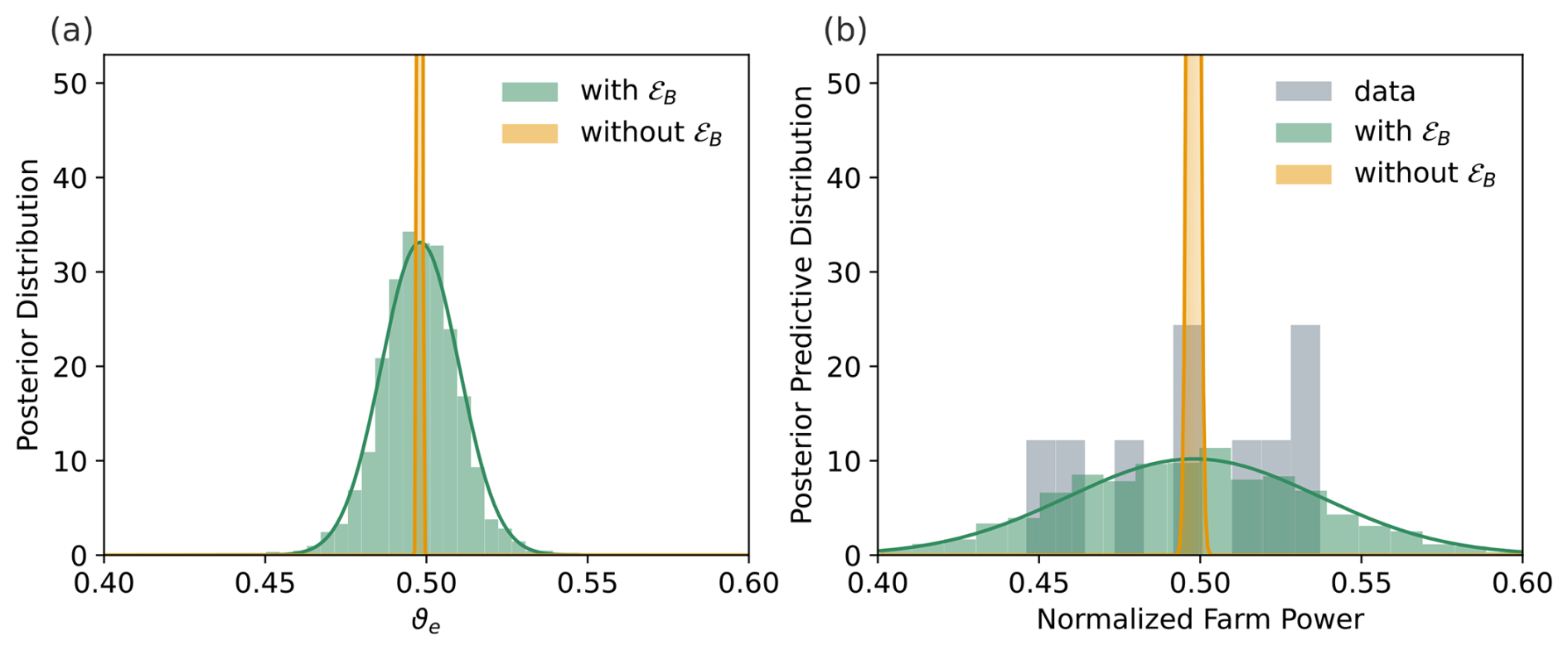
Figure 1 Comparison of the results of Bayesian UQ with and without the inclusion of model error ℰ_B: (a) posterior distribution and (b) posterior predictive distribution. The data and samples of the distributions obtained with UMBRA are given as histograms, and the analytically obtained probability density functions are given as full lines.

2.3.2 Posterior predictive distribution

The posterior predictive distribution for a new measurement ${\stackrel{\mathrm{̃}}{\mathcal{P}}}_{f,\text{new}}$ is given by

$$\begin{array}{}\text{(19)}& p\left({\stackrel{\mathrm{̃}}{\mathcal{P}}}_{f,\text{new}}|\mathcal{D}\right)=\mathcal{N}\left({\stackrel{\mathrm{̃}}{\mathcal{P}}}_{f,\text{new}};{\mathit{\mu }}_{N_D},{\mathit{\sigma }}_B^{\mathrm{2}}+{\mathit{\sigma }}_T^{\mathrm{2}}+{\mathit{\sigma }}_{N_D}^{\mathrm{2}}\right).\end{array}$$

The posterior predictive variance consists of the model error variance ${\mathit{\sigma }}_B^{\mathrm{2}}$, the measurement variance ${\mathit{\sigma }}_T^{\mathrm{2}}$, and the propagated posterior parameter variance ${\mathit{\sigma }}_{N_D}^{\mathrm{2}}$. If the model error is not included in the analysis, the posterior predictive underestimates the variance of the data both by neglecting ${\mathit{\sigma }}_B^{\mathrm{2}}$ and by underestimating ${\mathit{\sigma }}_{N_D}^{\mathrm{2}}$. Figure 1b shows that in the current example, the data do not seem plausible under the posterior predictive that neglects model error, rendering such a Bayesian analysis inadequate. The proper inclusion of model error through our framework yields an adequate posterior predictive and Bayesian analysis. Although the current example exhibits exceptionally large model uncertainty, most, if not all, of the current wind farm flow models have non-negligible model error, and Bayesian UQ analyses of such models that neglect model error will suffer similar issues.

2.3.3 Implications for stochastic flow models

Current stochastic wake models are obtained by propagating the posterior of the parameters – obtained by ignoring model error – through the model (Zhang and Zhao, 2020). They only account for the uncertainty on their parameters due to limited calibration data, and they do not capture the uncertainty due to varying unmodeled physics, such as stratification effects and time-resolved turbulence. Given enough data (here only 9 observations), they will therefore significantly underestimate the variability of the true process, as demonstrated in Fig. 1b. Moreover, in the limit of infinite data, such “stochastic” models will in fact become deterministic, as seen in Eqs. (18) and (19) with ${\mathit{\sigma }}_{N_D}\to \mathrm{0}$ and σ_B=0. Therefore, truly stochastic wind farm flow models should include both the posterior parameter uncertainty, quantified in p(ϑ_e|𝒟), and the model uncertainty, quantified through the model error covariance matrix Σ_B in the framework.

2.4 Sampling the posterior distribution

In practice, the analytical derivation of the moments and marginal distributions of the posterior distribution quickly becomes intractable. Instead, Markov chain Monte Carlo (MCMC) algorithms are typically used to efficiently sample the posterior distribution. With those samples, one can visualize the marginalized and joint posterior(s), consult the posterior predictive, and compute expected values. However, these algorithms are inherently serial and require 𝒪(10⁵) likelihood evaluations to converge to the posterior and adequately represent it (Geyer, 2011). Even for engineering models with reasonable computational expense, this can become relatively time-consuming. Therefore, we employ a variant of the transitional Markov chain Monte Carlo (TMCMC) algorithm (Ching and Chen, 2007), which is inherently parallel.

Instead of directly sampling the posterior distribution, TMCMC samples a sequence of target distributions with a sequential Monte Carlo (SMC) method. This sequence π_j(ϑ) is obtained by tempering the likelihood: a stage exponent or inverse temperature β_j is introduced that sequentially “cools” the target

$$\begin{array}{}\text{(20)}& {\displaystyle }{\displaystyle }{\mathit{\pi }}_j\left(\mathit{\vartheta }\right)\propto p\left(\mathcal{D}\right|\mathit{\vartheta }{)}^{{\mathit{\beta }}_j}p\left(\mathit{\vartheta }\right),\end{array}$$

where $j=\mathrm{1},\mathrm{\dots },J$ and $\mathrm{0}={\mathit{\beta }}_{\mathrm{1}}<\mathrm{\cdots }<{\mathit{\beta }}_J=\mathrm{1}$, such that the algorithm transitions from the prior (j=1), which is typically easy to sample from, to the posterior (j=J). This nomenclature stems from the analogy with the Boltzmann distribution $p\left(\mathit{\epsilon }\right)\propto \exp (-\mathit{\epsilon }/(k_B\mathrm{\Theta }\left)\right)$, which has high variance for high temperatures Θ and vice versa. The goal of the stage exponent is to gradually increase the influence of the likelihood by starting with an artificially large variance and then subsequently shrinking it. As a result, the algorithm can efficiently explore the prior range and successfully sample multimodal target distributions.

On the sequence of tempered target distributions, a particular version of the Resample–Move SMC algorithm is then used (Gilks and Berzuini, 2001; Doucet and Johansen, 2009), as depicted in Fig. 2. At every stage j, importance resampling is used to obtain N samples $\mathit{\{}{\mathit{\vartheta }}_j^{\left(k\right)}{\mathit{\}}}_{k=\mathrm{1}}^N$ that asymptotically follow the target distribution. To that end, importance weights are computed for every jth generation of particles:

$$\begin{array}{}\text{(21)}& {\displaystyle }{\displaystyle }w\left({\mathit{\vartheta }}_j^{\left(k\right)}\right)={\displaystyle \frac{p\left(\mathcal{D}\right|{\mathit{\vartheta }}_j^{\left(k\right)}{)}^{{\mathit{\beta }}_{j+\mathrm{1}}}p\left({\mathit{\vartheta }}_j^{\left(k\right)}\right)}{p\left(\mathcal{D}\right|{\mathit{\vartheta }}_j^{\left(k\right)}{)}^{{\mathit{\beta }}_j}p\left({\mathit{\vartheta }}_j^{\left(k\right)}\right)}}=p\left(\mathcal{D}\right|{\mathit{\vartheta }}_j^{\left(k\right)}{)}^{\mathrm{\Delta }\mathit{\beta }},\end{array}$$

where $\mathrm{\Delta }\mathit{\beta }={\mathit{\beta }}_{j+\mathrm{1}}-{\mathit{\beta }}_j$. Then the particles $\mathit{\{}{\mathit{\vartheta }}_j^{\left(k\right)}{\mathit{\}}}_{k=\mathrm{1}}^N$ are resampled with a probability

$$\begin{array}{}\text{(22)}& {\displaystyle }{\displaystyle }\mathbb{P}({\mathbf{\Theta }}_{j+\mathrm{1}}^{\left(k\right)}={\mathit{\vartheta }}_j^{\left(k\right)})={\displaystyle \frac{w\left({\mathit{\vartheta }}_j^{\left(k\right)}\right)}{{\sum }_{k=\mathrm{1}}^{N}w\left({\mathit{\vartheta }}_j^{\left(k\right)}\right)}}=\overline{w}\left({\mathit{\vartheta }}_j^{\left(k\right)}\right).\end{array}$$

Due to the importance sampling steps, the algorithm works best for priors that sufficiently cover the high-likelihood region. Since we employ wide weakly informative priors, this is almost always the case.

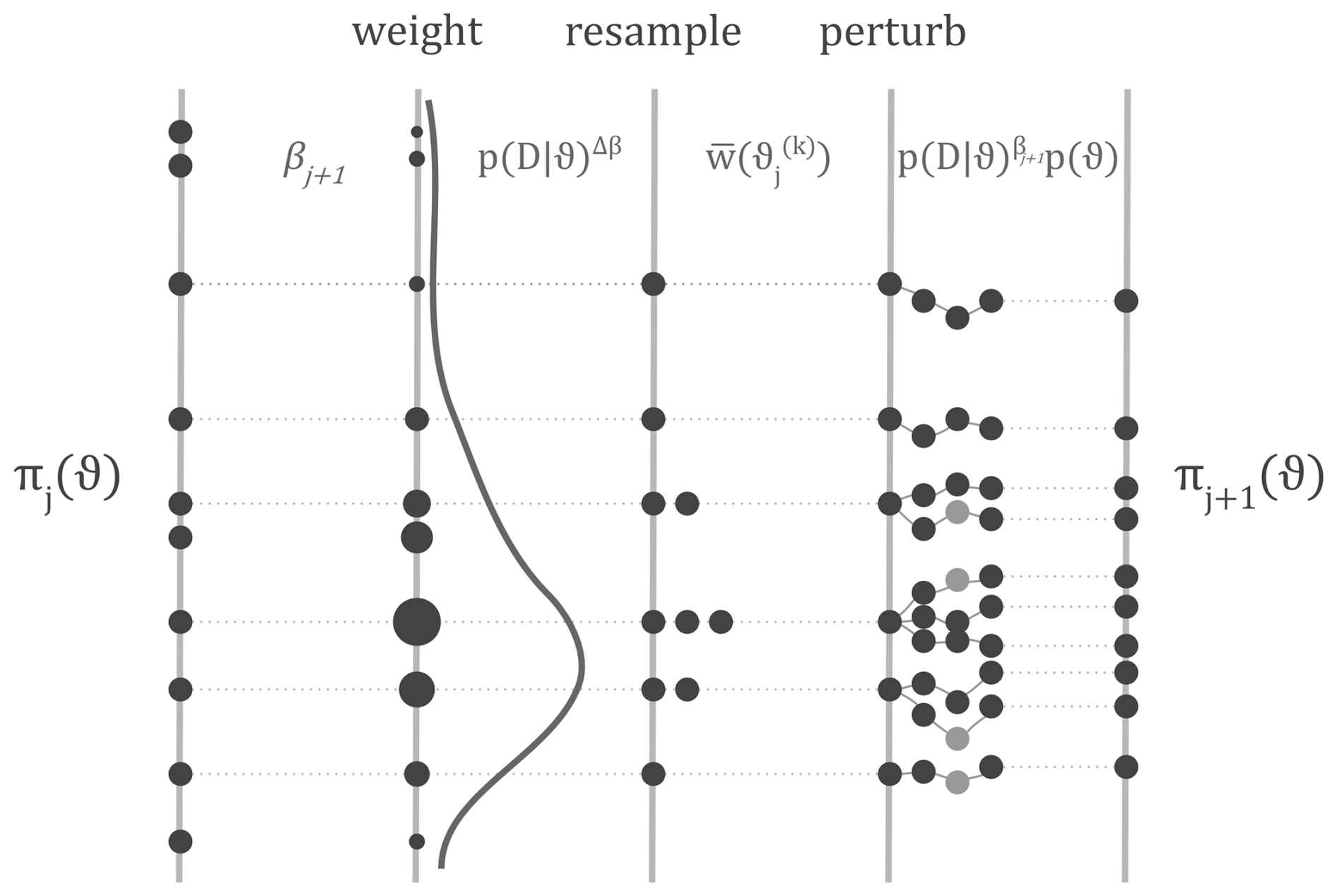
Figure 2 Schematic overview of one stage in the transitional Markov chain Monte Carlo (TMCMC) algorithm. From left to right, the samples are weighted, resampled, and perturbed. The algorithm can be parallelized in the perturbation phase. This figure is based on similar figures in the literature of sequential Monte Carlo and TMCMC (e.g., Doucet et al., 2001; Minson et al., 2013; Murphy, 2023).

Then N Metropolis–Hastings (MH) MCMC chains of length L are instantiated to perturb these samples again and remove the degeneracy introduced by the resampling step (Wu et al., 2018b). In the MH algorithm, the new sample ${\mathit{\vartheta }}_{j,l+\mathrm{1}}^{\left(k\right)}$ is sampled from a proposal density $q\left({\mathit{\vartheta }}_{j,l+\mathrm{1}}^{\left(k\right)}\right|{\mathit{\vartheta }}_{j,l}^{\left(k\right)})$ that only depends on the previous sample (Markov property). The new sample is accepted with a probability $min(\mathrm{1},{\mathit{\alpha }}_{\text{MH}})$, where the acceptance ratio α_MH is defined as

$$\begin{array}{}\text{(23)}& {\mathit{\alpha }}_{\mathrm{MH}}={\displaystyle \frac{{\mathit{\pi }}_j\left({\mathit{\vartheta }}_{j,l+\mathrm{1}}^{\left(k\right)}\right)}{{\mathit{\pi }}_j\left({\mathit{\vartheta }}_{j,l}^{\left(k\right)}\right)}}{\displaystyle \frac{q\left({\mathit{\vartheta }}_{j,l}^{\left(k\right)}\right|{\mathit{\vartheta }}_{j,l+\mathrm{1}}^{\left(k\right)})}{q\left({\mathit{\vartheta }}_{j,l+\mathrm{1}}^{\left(k\right)}\right|{\mathit{\vartheta }}_{j,l}^{\left(k\right)})}}.\end{array}$$

The Lth samples in the chains are taken as particle generation j+1. Since all MH chains can run simultaneously, the algorithm is inherently parallel. However, due to the MH steps, and thus similarly to (Adaptive) MH, TMCMC does not scale as well with parameter dimension as Hamiltonian Monte Carlo, which employs gradient information. If the prior does not sufficiently cover the high-likelihood region, longer MH chains are also required to compensate for the degeneracy introduced during importance sampling.

Several components of the algorithm can be tuned, such as the proposal distribution $q\left({\mathit{\vartheta }}_{j,l+\mathrm{1}}^{\left(k\right)}\right|{\mathit{\vartheta }}_{j,l}^{\left(k\right)})$ in MH, the method to determine β_j, the number of samples per stage N, and the number of MCMC steps L. In our case, the distribution of the MH proposal is multivariate normal, that is, $q\left({\mathit{\vartheta }}_{j,l+\mathrm{1}}^{\left(k\right)}\right|{\mathit{\vartheta }}_{j,l}^{\left(k\right)})=\mathcal{N}({\mathit{\vartheta }}_{j,l+\mathrm{1}}^{\left(k\right)};{\mathit{\vartheta }}_{j,l}^{\left(k\right)},{\mathbf{\Sigma }}_q)$, where Σ_q is the importance weighted sample covariance matrix of the previous stage scaled by $\mathrm{1}/\mathrm{9}+\mathrm{8}R/\mathrm{9}$, where R is the observed acceptance rate (Minson et al., 2013). The cooling rate should be fast enough to reduce the computational cost but slow enough to adequately represent the next target distribution after resampling. This adequacy can be quantified by the effective sample size (ESS) N^eff (Gelman et al., 2013). Its interpretation is that N weighted samples $\mathit{\{}{w}_j^{\left(k\right)},{\mathit{\vartheta }}_{j,L}^{\left(k\right)}{\mathit{\}}}_{k=\mathrm{1}}^N$ are worth N^eff i.i.d. samples drawn from the target distribution π_j+1 (Beck and Zuev, 2013). The ESS is estimated from the normalized importance weights as

$$\begin{array}{}\text{(24)}& {\displaystyle }{\displaystyle }{\widehat{N}}_{j+\mathrm{1}}^{\text{eff}}={\displaystyle \frac{\mathrm{1}}{{\sum }_k\overline{w}({\mathit{\vartheta }}_{j,L}^{\left(k\right)}{)}^{\mathrm{2}}}}={\displaystyle \frac{{\left({\sum }_{k}p\left(\mathcal{D}\right|{\mathit{\vartheta }}_{j,L}^{\left(k\right)}{)}^{\mathrm{\Delta }\mathit{\beta }}\right)}^{\mathrm{2}}}{{\sum }_{k}p\left(\mathcal{D}\right|{\mathit{\vartheta }}_{j,L}^{\left(k\right)}{)}^{\mathrm{2}\mathrm{\Delta }\mathit{\beta }}}}.\end{array}$$

The optimal cooling rate is obtained when β_j+1 is chosen such that the ESS is approximately half the total number of samples per stage (Minson et al., 2013). To that end, Eq. (24) is solved for β_j+1 with a bisection method on (β_j,1] (Kantas et al., 2014). Based on the study of the sensitivity of the posterior to the choice of N and L with increasing parameter dimension by Minson et al. (2013), we take N=1920 and L=20 for a total of (maximum) 10 parameters. For 15 stages, this requires 5.76×10⁵ likelihood evaluations, of which only 300 are inherently serial. For further details on the implementation, the reader is referred to the Python toolbox UMBRA, which is released together with this paper.

3 Case setup

The Bayesian UQ framework is demonstrated with a reference large-eddy simulation (LES) dataset for wind farm blockage and atmospheric gravity waves in conventionally neutral boundary layers (CNBLs). Since it is still challenging to model these effects with state-of-the-art models, the dataset provides a controlled setting for evaluating the framework under conditions of substantial model bias and uncertainty. The wind farm flow models are introduced in Sect. 3.1, and the dataset is described in Sect. 3.2. Based on the empirical model parameters and dataset characteristics, the prior distribution is further specified in Sect. 3.3.

3.1 Wind farm flow models

The two wind farm flow models we will consider in this study are a standard wake model (Sect. 3.1.1) and an atmospheric perturbation model (APM) (Sect. 3.1.2). The wake model cannot capture wind farm blockage and is expected to exhibit large model uncertainty for the considered dataset. The second model consists of a wake model with an APM-based blockage correction. Since the blockage effect in this dataset is mainly caused by atmospheric gravity waves, we opt for the APM as a blockage correction model, but different models exist (Branlard et al., 2020).

3.1.1 Standard wake model

The primary objective of wake models is to predict the effect of the velocity deficit downstream of a turbine on the other turbines within a farm. The most well-known and widely used wake model is presumably the one originally proposed by Jensen (1983), but over the years many others have followed (Göçmen et al., 2016). In this study, the Gaussian wake model of Bastankhah and Porté-Agel (2014) will be employed. It is based on the typical self-similar Gaussian profile of the velocity deficit and mass and momentum conservation in the wake (see also Frandsen et al., 2006).

The velocity deficit of a turbine i located upstream is then given by

$$\begin{array}{ll}{\displaystyle \frac{U_{\mathrm{\infty }}-U_{\mathrm{w}}\left(\mathit{x}\right)}{U_{\mathrm{\infty }}}}=& {\displaystyle }\left(\mathrm{1}-\sqrt{\mathrm{1}-{\displaystyle \frac{C_{T,i}}{\mathrm{8}{{\mathit{\sigma }}_i^{\ast }}^{\mathrm{2}}}}}\right)\\ \text{(25)}& {\displaystyle }& {\displaystyle }\times \exp \left(-{\displaystyle \frac{\mathrm{1}}{\mathrm{2}{{\mathit{\sigma }}_i^{\ast }}^{\mathrm{2}}}}{\displaystyle \frac{y^{\mathrm{2}}+z^{\mathrm{2}}}{D_i^{\mathrm{2}}}}\right)\mathcal{H}\left(x\right),\end{array}$$

where U_∞ is the free stream speed, U_w is the speed in the wake, and $\mathit{x}=[x,y,z{]}^{\top }$ is defined in a local coordinate system at the turbine hub, with z the vertical direction, z and y spanning the rotor plane, and x>0 downstream of the turbine. Furthermore, ℋ is the Heaviside function, C_T,i the turbine thrust coefficient, D_i is the rotor diameter, and ${\mathit{\sigma }}_i^{\ast }={\mathit{\sigma }}_i/D_i$ is the normalized wake width which grows linearly with the distance downstream from the rotor as

$$\begin{array}{}\text{(26)}& {\displaystyle }{\displaystyle }{\mathit{\sigma }}_i^{\ast }=k_{\mathrm{w}}{\displaystyle \frac{x}{D_i}}+\mathit{ϵ}.\end{array}$$

Here, k_w is the wake expansion rate, which is related to the local turbulence intensity at turbine with two empirical parameters as $k_{\mathrm{w}}=k_{a}I+k_b$, where a previous fit yielded $k_a=\mathrm{0.3837},k_b=\mathrm{0.003678}$ (Niayifar and Porté-Agel, 2016). Finally, ϵ is a semi-empirical parameter that represents the initial wake width, which depends on the turbine thrust coefficient (Bastankhah and Porté-Agel, 2014). The turbulence intensity at the turbine is determined with the method of Niayifar and Porté-Agel (2016) based on the original (Zehtabiyan-Rezaie and Abkar, 2023) expression for the added turbulence intensity expression by Crespo and Hernández (1996):

$$\begin{array}{}\text{(27)}& {\displaystyle }{\displaystyle }{I}_{+}=\mathrm{0.73}{a}^{\mathrm{0.8325}}{I}_{\mathrm{\infty }}^{-\mathrm{0.0325}}(x/D{)}^{-\mathrm{0.32}},\end{array}$$

where I_∞ is the background turbulence intensity.

In order to combine multiple wakes into one flow field a wake-merging method is needed. We will use the one developed by Lanzilao and Meyers (2022), which uses a self-similarity argument to combine the wake deficits through multiplication, without introducing any empirical parameters. Additionally, the turbines are mirrored to capture the effect of the ground plane (Lissaman, 1979). The power extracted by turbine i can then be computed as $P_i=\frac{\mathrm{1}}{\mathrm{2}}\mathit{\rho }{A}_i{U}_i^{\mathrm{3}}{C}_{P,i}\left(U_i\right)$, where C_P,i(U_i) is the power coefficient of that turbine, A_i is the swept rotor area, and U_i is the disk-averaged flow speed, calculated with the same quadrature method as in Allaerts and Meyers (2019).

3.1.2 Atmospheric perturbation model

Atmospheric perturbation models aim to model wind farm–atmosphere interaction effects such as wind farm blockage in addition to the turbine-scale interactions due to wakes. They do so by solving the height-averaged and linearized Reynolds-averaged Navier–Stokes (RANS) equations for the atmospheric boundary layer (ABL) under the Boussinesq approximation. The linearization involves adding a perturbation velocity $\mathit{u}=[u,v,w{]}^{\top }$ to the velocity $\mathit{U}=[U,V,W{]}^{\top }$ in the ABL. The APM further divides the ABL in a wind farm layer of height H₁ and a second layer of height $H_{\mathrm{2}}=H-H_{\mathrm{1}}$ where H is the ABL height. The equations and their solution procedures are derived and described in detail by Allaerts and Meyers (2019), Stipa et al. (2024a), and Devesse et al. (2024a). The three most important terms for our purposes are the farm thrust, the added turbulent momentum flux associated with the development of an internal boundary layer (IBL), and the pressure feedback induced by the upward displacement of the capping inversion layer – the interface between the neutral atmospheric boundary layer and the stably stratified free atmosphere aloft in CNBLs. Including this pressure feedback allows the APM to simulate the interaction between the ABL flow and gravity waves explicitly, thereby modeling blockage effects without introducing tuning parameters. The farm thrust and turbulent momentum flux, on the other hand, do contain parameters that will be calibrated with the Bayesian framework. Figure 3 represents these effects schematically.

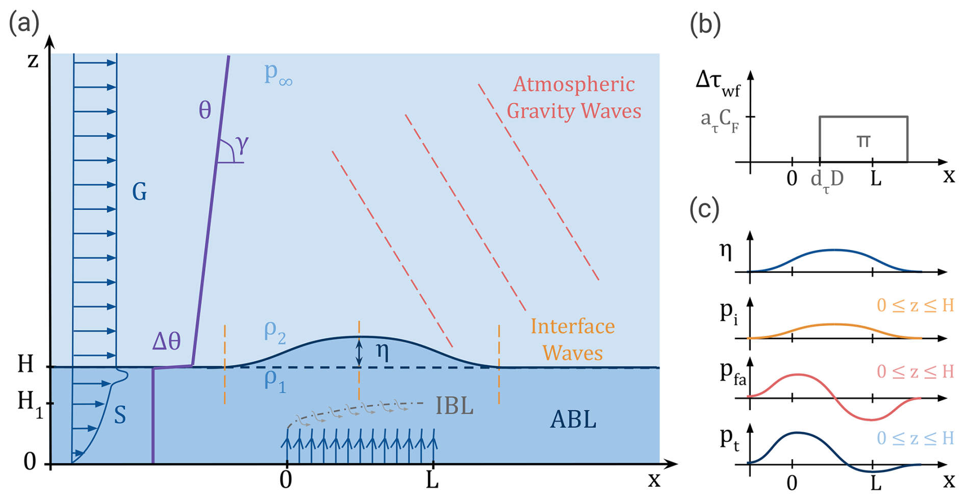
Figure 3 Schematic representation wind farm–atmosphere interaction via atmospheric gravity waves and internal boundary layer (IBL) development as modeled by the atmospheric perturbation model: (a) a sketch of the wind farm, vertical profiles of wind speed (blue) and potential temperature (purple), wave crests and troughs for internal gravity waves in the free atmosphere (red) and interface waves on the inversion layer (orange), and a developing IBL (gray); (b) the added momentum flux due to the presence of the wind farm and related to IBL growth as modeled in the APM; (c) a hypothetical displacement η of the inversion layer with the associated pressure feedback p_t in the atmospheric boundary layer (ABL), split up in the pressure components related to the waves on the inversion layer p_i, and the waves in the free atmosphere p_fa.

The wind farm thrust f(x,y) is represented in the APM by filtering the turbine thrust forces f_i located at the turbine positions (Allaerts and Meyers, 2019)

$$\begin{array}{}\text{(28)}& \begin{array}{rl}\mathit{f}(x,y)& =\underset{\mathrm{0}}{\overset{L_x}{\int }}\underset{\mathrm{0}}{\overset{L_y}{\int }}G(x-x^{\prime },y-y^{\prime })\\ & \times \sum _{i=\mathrm{1}}^{N_{\mathrm{T}}}{\mathit{f}}_i\mathit{\delta }(x^{\prime }-x_i,y^{\prime }-y_i)\mathrm{d}{x}^{\prime }\mathrm{d}{y}^{\prime },\end{array}\end{array}$$

for an APM domain of $[\mathrm{0},L_x]\times [\mathrm{0},L_y]$. Here, δ(x,y) is the two-dimensional Dirac delta and G(x,y) is a Gaussian filter kernel with a filter length scale of L_f

$$\begin{array}{}\text{(29)}& {\displaystyle }{\displaystyle }G(x,y)={\displaystyle \frac{\mathrm{1}}{\mathit{\pi }{L}_{\mathrm{f}}^{\mathrm{2}}}}\exp \left(-{\displaystyle \frac{x^{\mathrm{2}}+y^{\mathrm{2}}}{L_{\mathrm{f}}^{\mathrm{2}}}}\right).\end{array}$$

The filter length scale is set to 1000 m by Allaerts and Meyers (2019) and Devesse et al. (2024a) and to 500 m by Stipa et al. (2024a), and it can be considered an uncertain parameter. This filtering operation must be applied to the momentum equations as a whole, resulting in dispersive stresses (Devesse et al., 2024a). However, computing the resulting dispersive stresses with the current parametrization is the most expensive part of an APM evaluation (Devesse et al., 2024b). Since these stresses are a minor perturbing force compared to the turbine thrust, we will ignore them to reduce the computational cost. Faster parametrizations for the dispersive stresses in the APM are a topic of ongoing research.

The development of an internal boundary layer is accompanied by an increase in the momentum flux from the layer above the wind farm to the wind farm layer. This added turbulent momentum flux is represented as (Devesse et al., 2024a)

$$\begin{array}{}\text{(30)}& {\displaystyle }{\displaystyle }\mathrm{\Delta }{\mathit{\tau }}_{\text{WF}}(x,y)=a_{\mathit{\tau }}{C}_{\mathrm{F}}\mathrm{\Pi }(\mathbf{\text{x}}-d_{\mathit{\tau }}D{\mathit{e}}_{\mathrm{s}}),\end{array}$$

where a_τ is the proportionality constant to the wind farm force density $C_{\mathrm{F}}=\frac{\mathrm{1}}{\mathrm{2}}{C}_{\mathrm{T}}{N}_{\mathrm{T}}A\left|\right|{\mathit{U}}_{\mathrm{1}}|{|}^{\mathrm{2}}/S_{\mathrm{F}}$ and e_s is the streamwise unit vector. Here, C_T is the average turbine thrust coefficient, N_T is the number of turbines, A is the swept rotor area, U₁ is the unperturbed velocity in the farm layer, and S_F is the wind farm surface. The added momentum flux is oriented along the wind farm forcing and is zero everywhere except on the wind farm footprint Π(x). For a rectangular farm, this is a block function. To include the development of the IBL, the footprint is shifted d_τ turbine diameters downstream given that the turbines that are on average aligned with the wind. That leaves two empirical parameters a_τ and d_τ, which were previously fitted to 0.12 and 27.8 based on the computed added momentum flux from LES data (Devesse et al., 2024a).

The farm thrust will slow down the flow in the ABL. The resulting decrease in the streamwise velocity u is balanced in the continuity equation by induced spanwise flow v and thickening of the ABL. This thickening corresponds to a lifting of the capping inversion η, which leads to two distinct processes that result in the pressure feedback $p_t=p_i+p_{\text{fa}}$ (cf. Fig. 3c). First, the lifting of the capping inversion directly corresponds to a cold anomaly, as the air below it is colder than the air above. These pressure perturbations p_i can travel horizontally along the capping inversion as two-dimensional interfacial gravity waves. Second, the changes in capping inversion height perturb the free atmosphere aloft, leading to internal gravity waves. These three-dimensional waves also lead to pressure perturbations, which are felt throughout the ABL (Smith, 2010). Combined, these two types of gravity waves cause a pressure increase upstream, leading to the blockage effect. Downstream, they also induce a favorable pressure gradient throughout the farm (cf. Fig. 3c).

The wake effects are included with a standard wake model, which can be coupled to the height-averaged RANS equations for the two layers together with the pressure feedback from the upper atmosphere (Devesse et al., 2024b). The predicted flow redirection is included with a simplified version of the bidirectional wake-merging method of Lanzilao and Meyers (2022), which is elaborated upon in Appendix A. In the current work, the wake model is coupled via the pressure (Stipa et al., 2024a), but an upstream coupling (Allaerts and Meyers, 2019) and a velocity matching approach exist as well (Devesse et al., 2024a). Figure 4 shows the obtained flow field, where the wake model provides the information on the wakes and the APM provides the background velocity and pressure information.

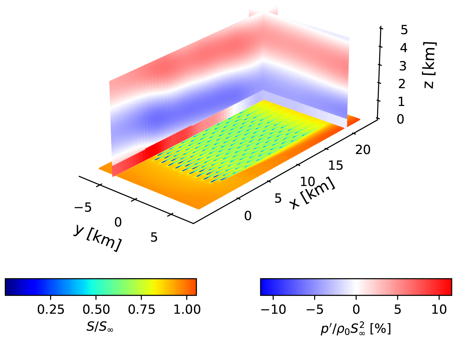
Figure 4 Wind speed and pressure field obtained with an atmospheric perturbation coupled via the pressure to a Gaussian wake model with a bidirectional wake-merging method. The staggered wind farm consists of 16 rows of 10 wind turbines with streamwise and spanwise spacings of 5 rotor diameters. The atmospheric boundary layer height amounts to 500 m with a capping inversion strength of 4 K and a free-atmosphere lapse rate of 8 K km⁻¹. The friction velocity equals 0.275 m s⁻¹. The upstream wind speed and ambient turbulence intensity at hub height are 9.24 m s⁻¹ and 3.93 %.

3.2 Reference dataset

As reference data, the parametric LES study of wind farm blockage and gravity waves in CNBLs of Lanzilao and Meyers (2024) is used. They simulated 36 selected atmospheric states based on 30 years of ERA5 re-analysis data at the nearest grid point to the Belgian–Dutch offshore wind farm cluster. Figure 5 depicts the inflow conditions (the time average of the last 4 h of the precursor simulations) and the power output per turbine, normalized by the power of a hypothetical undisturbed turbine upstream, for the cases with an ABL height of 500 m. From Fig. 5b it can be seen that the ABL is always neutrally stratified, since the potential temperature θ remains constant $\mathrm{d}\mathit{\theta }/\mathrm{d}z=\mathrm{0}$. The capping inversion strength Δθ, and the lapse rate in the free atmosphere aloft $\mathrm{d}\mathit{\theta }/\mathrm{d}z>\mathrm{0}$ are varied.

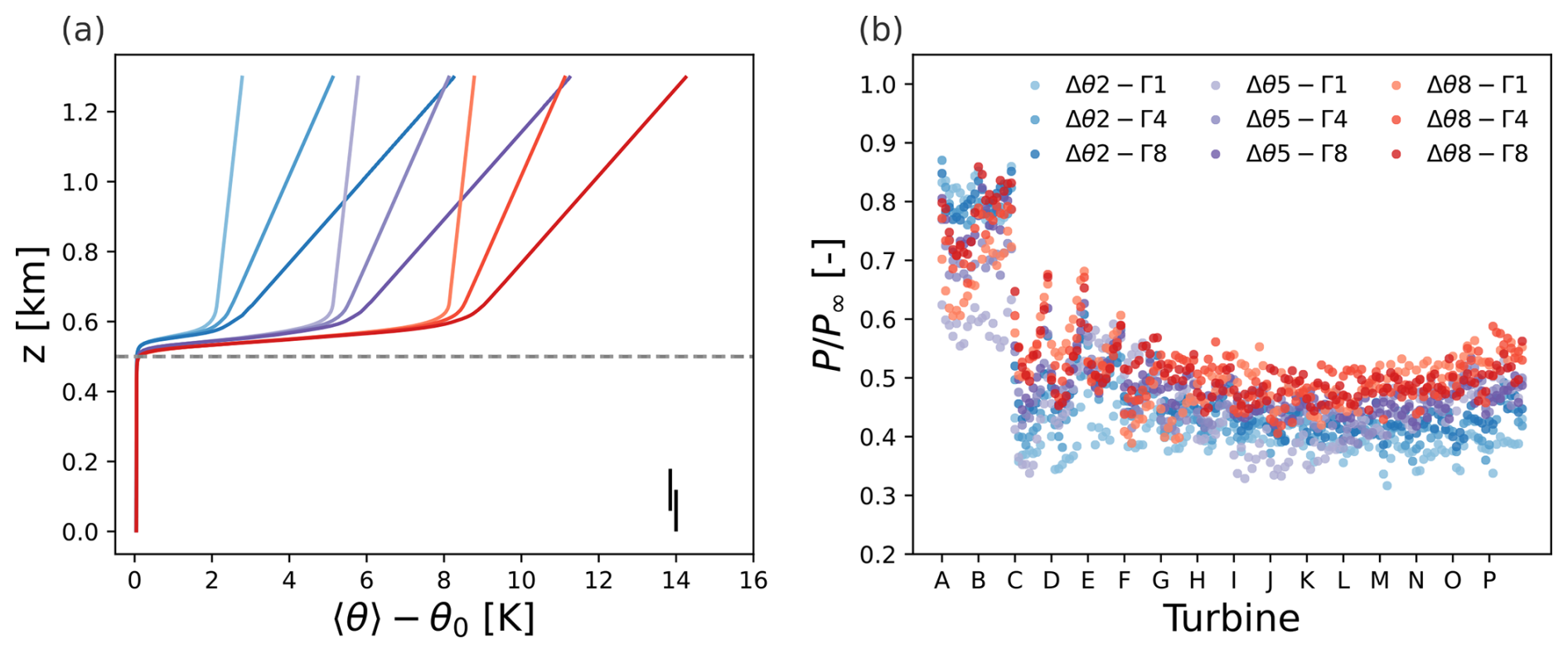
Figure 5 Large-eddy simulation data of Lanzilao and Meyers (2024): (a) potential temperature profile with θ₀=288.15 K, averaged horizontally in space and over the last 4 h of the precursor simulation, and (b) power output per turbine normalized by the power of an “undisturbed” upstream turbine. In panel (a), the ABL height is indicated with a dashed gray line and a turbine is drawn with full black lines as a reference.

The wind farm consists of 16 rows and 10 columns (N_T=160) of 10 MW IEA reference turbines (Bortolotti et al., 2019). The streamwise and spanwise spacings are 5D, with D=198 m as the turbine diameter. The turbines have hub heights of z_h=119 m, and in the study the thrust coefficient is fixed to C_T=0.88. The rows are counted in the streamwise direction and labeled with capital letters in Fig. 5b. It can be seen in Fig. 5b how the blockage effect causes large reductions in turbine power in the first rows. At the same time, the favorable pressure gradient improves power recovery in the last rows. The significant local flow redirection related to blockage misaligns the turbine wakes with the downstream turbines on the sides of the farm, resulting in a U-shaped trend in the power per row. In general, the resulting turbine power output varies significantly with atmospheric stratification.

Of the 36 available cases, we will only consider the 9 cases with an ABL height of 500 m in this study, to isolate the effect of stratification of the upper atmosphere from the height of the boundary layer. As we intend to demonstrate the framework's capability to quantify the uncertainty adequately for models of different fidelity, the APM is included as a model. However, an APM evaluation takes about 30 s, so 1000 model evaluations already require 8.3 core hours, compared to 0.83 core minutes for 1000 wake–model evaluations of 0.05 s. Although the SMC algorithm allows the many required APM evaluations to be performed in parallel to achieve a speed-up in time, the total computational cost remains the same.

3.3 Prior choices depending on the dataset and models

An overview of the marginal priors for the empirical model parameters ϑ_e of the wake model and the APM, as well as the parameters ${\mathit{\vartheta }}_b=\mathit{\{}{\mathit{\delta }}_{\mathit{\zeta }},{\mathit{\sigma }}_{B,\mathit{\zeta }}{\mathit{\}}}_{\mathit{\zeta }=\mathrm{0}}^{{\mathit{\zeta }}_{\text{max}}}$ that characterize the model error distribution, is given in Table 1. The measurement error covariance can be calculated from the 90 min long turbulent power signals using the moving block bootstrap (Garcia et al., 2005). Since the upstream velocity and potential temperature profiles are available from the LES, the inflow uncertainty is considered negligible. The prior of the mean bias terms depends on the considered wind farm flow model in the adapted Bayesian framework. For the wake model, we know a priori that the sensitivity of the predicted power to the wake expansion rate is only zero for the upstream turbines, which are not waked. Therefore, only the bias in the upstream and undisturbed rows of turbines δ₀ can be nonzero based on the condition against confounding of the model bias with calibration parameters in Eq. (10). However, we find that also requiring δ₀=0 works best in practice based on a comparison of alternatives in Sect. 4.1. For the APM, the condition for the best-fit interpretation of the model parameters in Eq. (10) directly requires that all mean bias terms δ_ζ(i) are zero.

Table 1 Prior distributions for the inverse uncertainty quantification of the wake model and the atmospheric perturbation model. Uniform distributions on an interval [a,b] are abbreviated as ${\mathcal{U}}_a^b$. The exponential distribution Exp_λ has a PDF $p\left(x\right)={\mathit{\lambda }}^{-\mathrm{1}}\exp (-x/\mathit{\lambda })$ for x>0. The Dirac delta distribution Delta(a) has a PDF $p\left(x\right)=\mathit{\delta }(x-a)$. The filter length L_f and height of the first layer H₁ are expressed in meters, and the spatial delay of the turbulent entrainment d_τ is expressed in turbine rotor diameters.

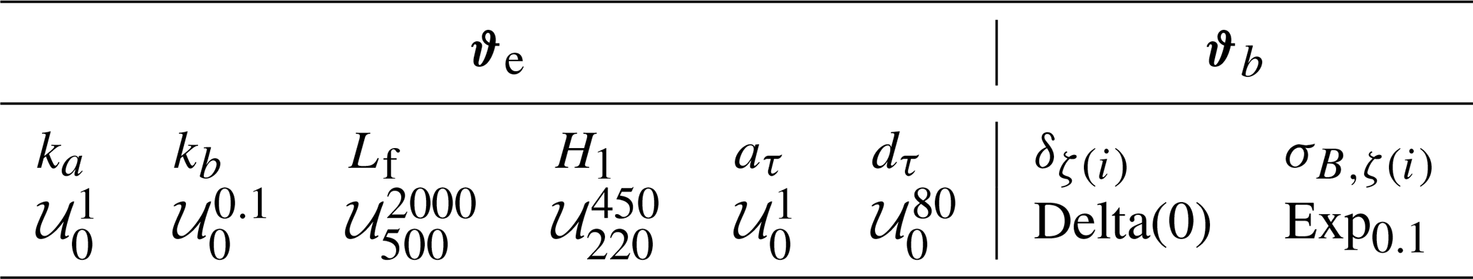
The model parameters are given by ${\mathit{\vartheta }}_{\mathrm{e}}=(k_a,k_b)$ for the wake model and by ${\mathit{\vartheta }}_{\mathrm{e}}=(k_a,k_b,L_{\mathrm{f}},H_{\mathrm{1}},a_{\mathit{\tau }},d_{\mathit{\tau }})$ for the APM. Similarly to previous work (Aerts et al., 2023), the wake expansion rate parameter k_a gets a uniform prior over the unit interval, whereas k_b gets a stronger uniform prior between 0–0.1. These marginal priors for k_a and k_b ensure that the wake expansion rate is positive for all turbulence intensities. The filter length scale L_f is taken not smaller than the grid spacing of 500 m and not larger than 2 times the current value in Devesse et al. (2024a). The allowable farm layer height H₁ is chosen slightly larger than the turbine tip height of 218 m and smaller than 90 % of the ABL height of 500 m. The strength a_τ of the turbulent entrainment should be positive and is not expected to be more than 10 times larger than its current estimated value of ≈0.1 (Devesse et al., 2024a). The spatial delay of the turbulent entrainment d_τ should clearly be positive and cannot exceed the farm length of 80 turbine diameters.

4 Results and discussion

In Sect. 4.1, the adequacy of the Bayesian framework is verified for the wake model, which is expected to show large model error and uncertainty for the blockage dataset, and the APM, which is expected to perform better. The posterior distributions for both models are compared in Sect. 4.2. Lastly, the generalization of the results and the intended use of the framework are discussed in Sect. 4.3. The posterior distributions are sampled on the wICE supercomputing platform of the VSC (Vlaams Supercomputer Centrum), using Sapphire Rapids nodes containing 2 Intel Xeon Platinum 8468 CPUs (48 cores each).

4.1 Adequacy of the Bayesian framework

We now turn to the analysis of the wake model and the APM with turbine power data. Since the posterior distribution is intractable for those cases, we use the parallelized SMC algorithm implemented in UMBRA to sample it (Sect. 2.4). The SMC algorithm yields 1920 samples of the joint posterior distribution of ϑ_e and ϑ_b after convergence. In addition, we generate a sample of the posterior predictive distribution for each sample of the posterior so that the adequacy of the Bayesian framework can be assessed by comparing the posterior predictive samples with the observations (Sect. 2.2.2).

Figure 6 compares the means and standard deviations of the posterior predictive samples of each turbine with the distribution of the LES reference data for both the wake model and the APM. To isolate model uncertainty from (epistemic) parameter uncertainty and measurement uncertainty, we also show the posterior predictive obtained from the same posterior of the model parameters, but with $\mathit{\{}{\mathit{\sigma }}_{B,\mathit{\zeta }\left(i\right)}{\mathit{\}}}_{i=\mathrm{1}}^{N_{\mathrm{T}}}$ set to zero. Figure 6a shows that the wake model exhibits substantial model uncertainty for this dataset. In the first turbine rows, the model uncertainty is inflated because of the significant bias due to wind farm blockage. Further downstream, the large model uncertainty stems form the U-shaped power variations caused by flow redirection and the enhanced power recovery due to the favorable pressure gradient, which the wake model fails to capture. Notably, the data appear implausible under the posterior predictive without model error, underscoring the importance of properly accounting for model uncertainty. Figure 6b shows that the APM yields considerably lower model uncertainty, as it successfully incorporates blockage, flow redirection, and pressure gradient effects. However, consistent with previous findings (Devesse et al., 2024b), the APM underestimates blockage effects in the first rows, which inflates model uncertainty for those turbines. Since the reference data are deemed plausible under the posterior predictive distributions of both models, the Bayesian framework proves to be adequate.

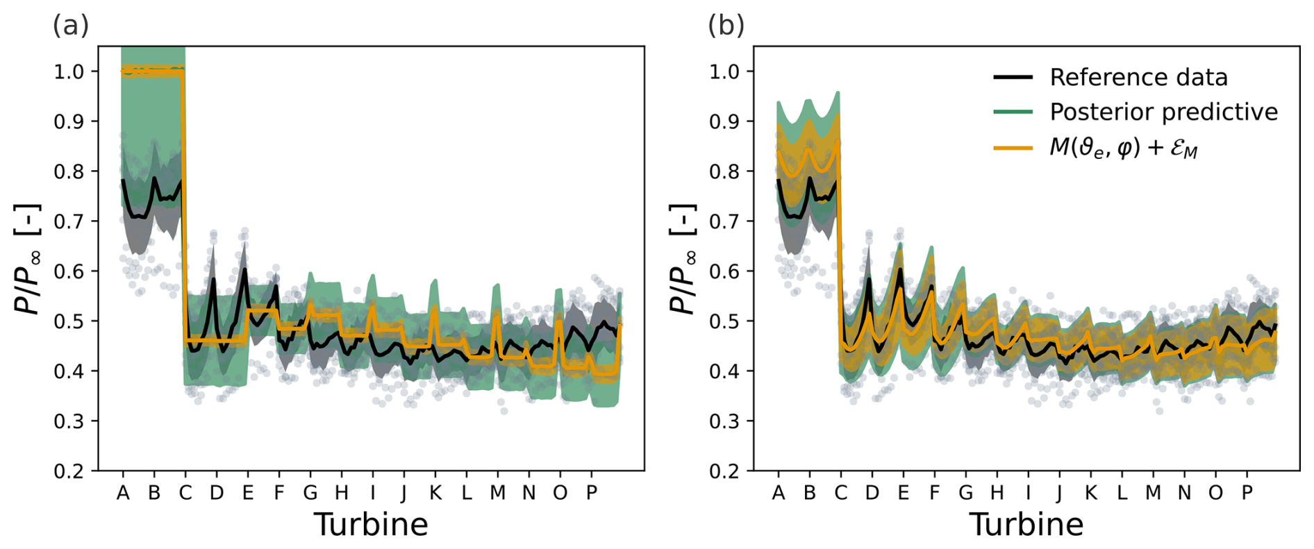
Figure 6 Comparison of the turbine power from LES with the posterior predictive distributions for (a) the wake model and (b) the atmospheric perturbation model. The mean power is shown as a solid line, with shaded regions indicating 1 standard deviation above and below the mean. The mean and standard deviation of the model outputs M(ϑ_e,φ) for the posterior samples of ϑ_e are shown as well after adding the measurement error 𝓔_M. The reference data points are also plotted as individual dots.

To avoid overestimating model uncertainty caused by systematic model mismatch, one could also estimate the mean model bias. However, this bias must be constrained to ensure model parameter identifiability, either by enforcing unbiased predicted farm power in Eq. (9) or by trivially satisfying the condition against confounding of the model bias with model parameters in Eq. (10). One approach is to relax the condition for the “best-fit” parameter interpretation in Eq. (10), as illustrated in Fig. 7a for the wake model. This allows the mean bias δ₀ to be identified in the first turbine rows due to blockage, resulting in lower estimated model uncertainty. However, to compensate for this bias and still match farm power, the calibrated wake model systematically underestimates turbine power downstream. Alternatively, we can relax the constraint that predicted farm power must be unbiased, as shown in Fig. 7b for the wake model. This yields the exact same calibration (and posterior of the model parameters) as when the mean bias for the upstream turbines is not estimated, since upstream power contains no information about the model parameters. Nevertheless, as Fig. 6b shows, even flow models that have parameters that influence the predicted blockage effect can exhibit bias, leading to inflated uncertainty estimates for these models. Therefore, we recommend excluding mean model bias to enable the objective comparison of model uncertainty between different flow models, even though the estimated model uncertainty is conservative.

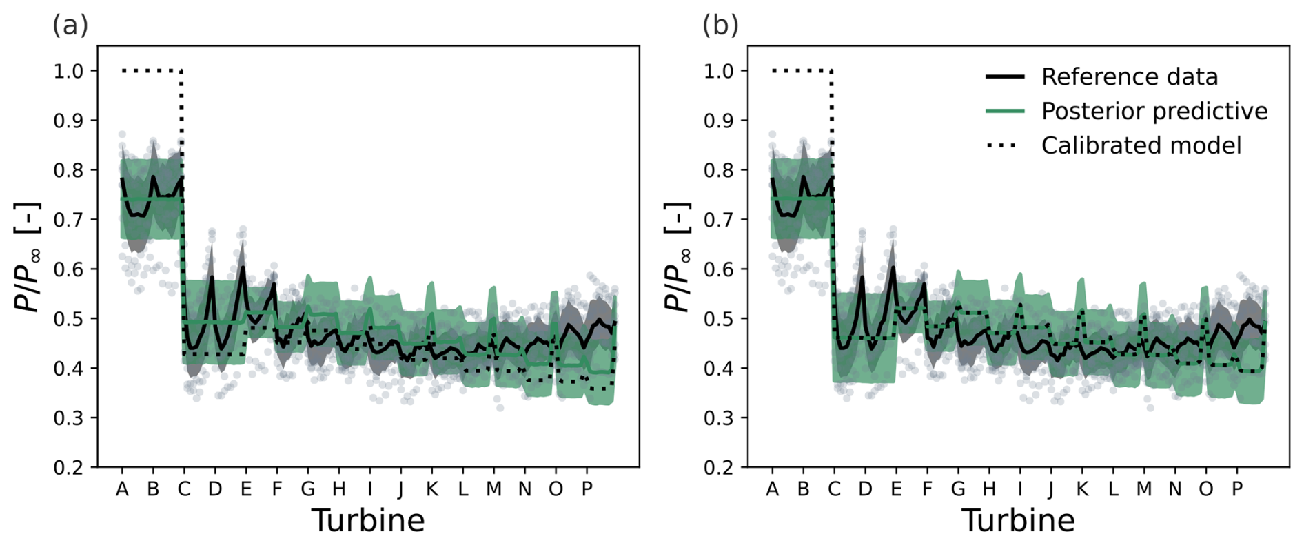
Figure 7 Comparison of the turbine power data from LES with the posterior predictive distribution for the wake model when the mean bias terms μ_B,i are estimated together with the model parameters. In panel (a), all mean bias terms are estimated with the constraint that their sum is zero, whereas in panel (b) only the bias on the upstream turbines is estimated. The mean power is shown as a solid line, with shaded regions indicating 1 standard deviation above and below the mean. The reference data points are also plotted as individual dots.

4.2 Model comparison with quantified model and parameter uncertainty

The Bayesian UQ framework can be used to perform objective model comparison with quantified parameter and model uncertainty given a reference dataset. In Sect. 4.2.1, the posterior distributions of the model parameters are presented for the wake model and the atmospheric perturbation model. The posterior distribution of the parameters describing the model error distribution are compared for both models in Sect. 4.2.2.

4.2.1 Posterior distribution of the model parameters

Figure 8 shows one- and two-dimensional histograms of the joint posterior distribution of the wake model parameters, based on samples generated with SMC in UMBRA and visualized with Corner (Foreman-Mackey, 2016). A comparison between the marginal posterior and prior distributions reveals that the parameters are well identified. Notably, the posterior median of k_a (0.52) exceeds its standard reference value of 0.384 (Niayifar and Porté-Agel, 2016), while k_b is estimated to be nearly zero. In rows A and B, where turbines are not affected by wakes, the mean posterior wake expansion rate $k_{\mathrm{w}}=k_{a}I+k_b$ is approximately 0.018, given an ambient turbulence intensity of 0.039, compared to 0.019 based on the same turbulence intensity I and literature values for k_a and k_b. In the downstream rows, the mean posterior wake expansion rate increases to around 0.073 due to wake-added turbulence, compared to a literature-based value of 0.064 using the same local turbulence intensity. This suggests that wake recovery in waked turbine rows is overestimated to compensate for the favorable pressure gradient influencing the background flow field. Although the estimated wake expansion rate in the upstream rows is consistent with earlier results, the local wind speed is largely overestimated by the wake model, which makes the comparison invalid.

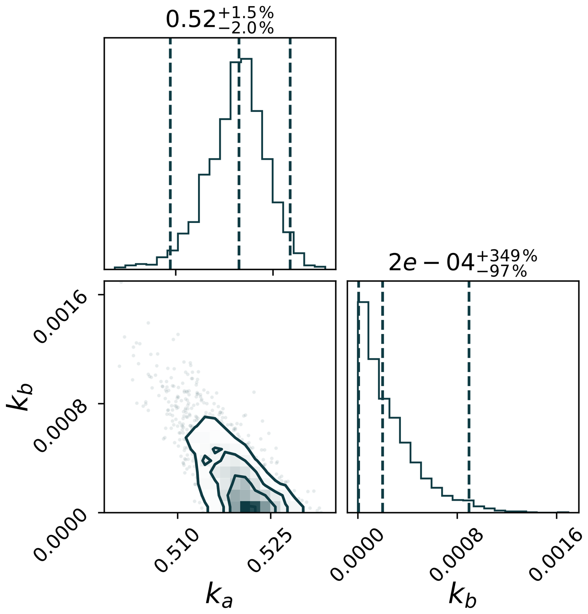
Figure 8 Joint posterior probability density of the parameters in the wake expansion rate $k_{\mathrm{w}}=k_{a}I+k_b$. For each parameter, the median is given together with the 2.5 % and 97.5 % quantiles, expressed as relative deviations from the median.

Figure 9 shows the samples of the joint posterior distribution of the APM parameters, which are all well identified. Compared to standard values, the posterior median of k_a is lower (0.32) and that of k_b is higher (0.0125), resulting in a larger mean wake expansion rate in rows A–B (k_w≈0.027) and a similar rate in the downstream rows (k_w≈0.064), given the same turbulence intensities. The increased upstream wake expansion rate suggests the need for further investigation into turbine wakes under blockage conditions (see Ndindayino et al., 2025). The estimated filter length scale L_f is smaller than the value used in Devesse et al. (2024a) but slightly larger than in Stipa et al. (2024a). The relatively high uncertainty in L_f is attributed to the limited sensitivity of the turbine power to changes in filter width between 500 m and 640 m. The height of the first layer H₁ is estimated to be close to twice the turbine hub height, consistent with findings from a previous parameter study (Allaerts and Meyers, 2019). The estimated strength of the wind farm added momentum flux a_τ reaches the upper bound of its prior, roughly 10 times its current value, and its spatial delay d_τ is larger than previously fitted. This discrepancy across the model chain indicates that the parametrization of the added momentum flux requires further refinement. In the pressure-based coupling of the wake model to the height-averaged RANS equations, noticeable increases in turbine power only occur for a_τ values near 1. Thus, the strong added momentum flux downstream helps to replicate the observed power increase in rows N–P (cf. Fig. 6b).

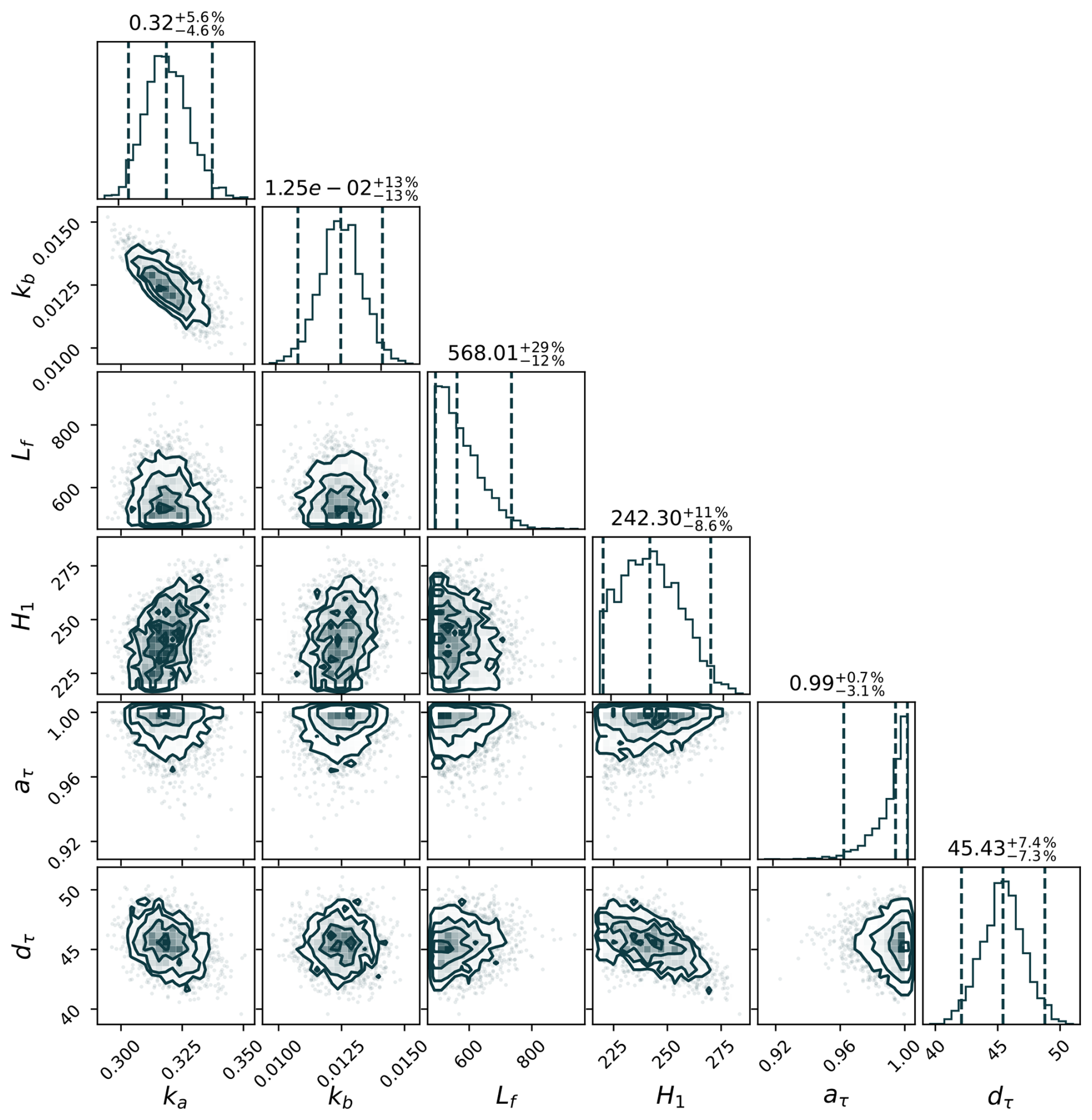
Figure 9 Joint posterior probability density of the parameters in the atmospheric perturbation model. For each parameter, the median is given together with the 2.5 % and 97.5 % quantiles, expressed as relative deviations from the median.

4.2.2 Comparison of the quantified model uncertainty

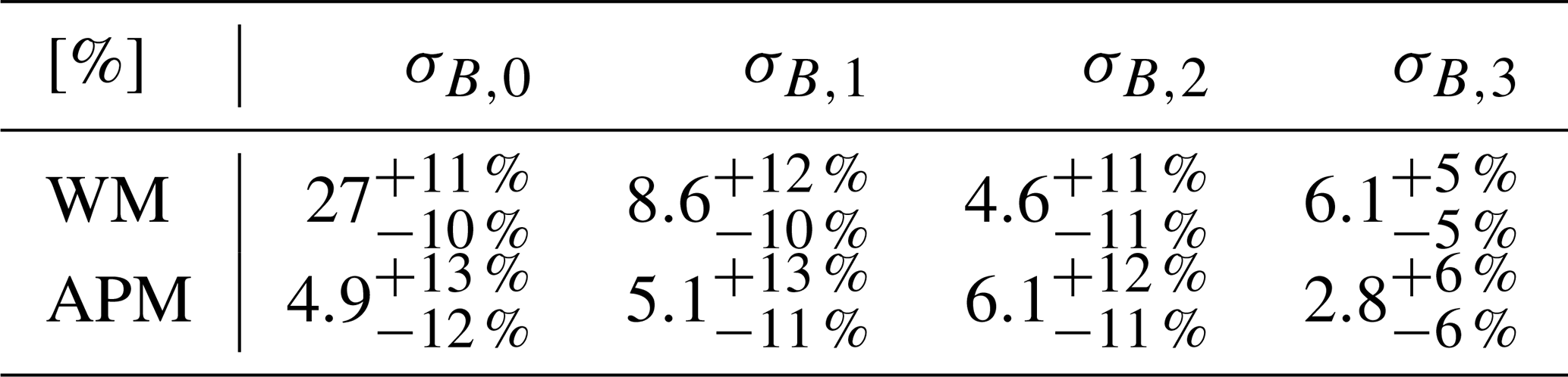
Table 2 summarizes the marginal posteriors of the model error standard deviations for both wind farm flow models. It is clear that the rather large uncertainties σ_B,ζ(i) for the wake model are caused by the unobserved or unmodeled variations in atmospheric stratification in this dataset. In general, the model uncertainty is smaller for the APM, as the standard deviations of the model error σ_B,ζ(i) are smaller. Because the APM captures the blockage effect, the model uncertainty on upstream turbines is reduced by a factor of 5.5 for this dataset. In addition, variations in upstream blockage are better estimated, as the uncertainty of the turbines with one waking turbine is lowered by a factor of 1.5. Only the model uncertainty for turbines with two upstream waking turbines is larger. In fact, it is seen in Fig. 6 that the deviations from the predicted power are larger in rows E and F. In contrast, the model uncertainty σ_B,3 for turbines farther downstream is a factor of 2.2 lower than for the wake model. This is because the APM adequately models the increase in power in later rows due to the inclusion of the favorable pressure gradient and the wind farm added momentum flux. Note that the posterior uncertainty on σ_B,3 is smaller than on the other model error standard deviations. This is because σ_B,3 is associated with 100 turbines, while the others are associated with 20 only. Thus, its epistemic uncertainty is further reduced by a factor $\sqrt{\mathrm{5}}$.

Table 2 Summary statistics of the marginal posterior distributions of the model error standard deviation σ_B,ζ(i) for the wake model (WM) and the atmospheric perturbation model (APM). For each parameter, the median is given together with the 2.5 % and 97.5 % quantiles, expressed as relative deviations from the median.

4.3 Generalization of the obtained results

A natural question that arises when calibrating models is to what extent the resulting performance generalizes to other datasets. Since physics-based wind farm flow models are expected to generalize well to other farm layouts, wind speeds, and wind directions, we expect that the performance should generalize well when varying those conditions. In that case the posterior distribution of the empirical parameters p(ϑ_e|𝒟) can be used together with the quantified model error distribution to obtain a stochastic wind farm flow model. However, for unobserved or unmodeled conditions ψ^′, we cannot expect a proper generalization, since the bias of the flow model can only (partially) be reduced by altering the empirical model parameters ϑ_e. Consequently, the results of the uncertainty quantification depend largely on the resemblance between the distribution of these unobserved conditions in the considered data p(ψ^′) and their true distribution p_true(ψ^′). In this case, we have by no means covered the true distribution p_true(ψ^′) – even if we intended to consider only atmospheric stratification effects in CNBLs with an ABL height of 500 m. Similarly, the posteriors of the model parameters likely depend on the ABL height. As such, the obtained results are specific to the dataset considered and are intended only as an illustration of the methodology. However, we showed that the methodology does allow objective model comparison with quantified model and parameter uncertainty given a benchmark dataset.

5 Summary and outlook

Bayesian UQ leverages data to quantify the uncertainty of model parameters and the model itself by updating a prior distribution that characterizes the available knowledge, before having seen the data, to a posterior distribution. In this article, we examined the use of Bayesian UQ for (1) obtaining stochastic wind farm flow models through Bayesian calibration and (2) objective model comparison with quantified parameter and model uncertainty. As both applications require that model inadequacy is properly taken into account, the model inadequacy formulation in a previously developed Bayesian UQ framework (Aerts et al., 2023) was improved. The framework was demonstrated with engineering models for wind farm–atmosphere interaction using a large-eddy simulation dataset for wind farm blockage due to atmospheric gravity waves. In doing so, the framework was tested for delineated data with a large anticipated model uncertainty, as current engineering models face difficulties in representing those effects. In contrast to earlier studies, we used a parallelized sequential Monte Carlo algorithm based on likelihood tempering to speed up the approximation of the posterior, though at a similar computational cost. This complete workflow is made available in a Python toolbox coined Uncertainty Modeling toolbox for Bayesian data Re-Analysis (UMBRA), which can be used together with WAYVE (Devesse et al., 2023) and WIFA (Quick et al., 2024).

With a simple example model for wind farm power, the consequences of not properly including model error in Bayesian UQ are illustrated. On the one hand, the posterior distribution of the model parameters is overconfident and biased when the model error is neglected. In that case, a posterior predictive check also shows that the Bayesian analysis is inadequate. Hence, the proper inclusion of model error is also important when one is only interested in the posterior distribution of the flow model parameters. On the other hand, current stochastic flow models, which only propagate the posterior distribution of the model parameters through the model (Zhang and Zhao, 2020), may significantly underestimate the variability of the true process that the model aims to represent, as soon as there is non-negligible model error. Moreover, in the limit of infinite data, such “stochastic” models will, in fact, become deterministic. The presented framework properly includes the model error so that the posterior distribution of the model parameters and the model uncertainty are adequately quantified, also in the limit of infinite data. Since most, if not all, of the current wind farm flow models have non-negligible model error, Bayesian UQ analyses that neglect model error will suffer similar issues.

The adequacy of incorporating model error on turbine power predictions within the Bayesian framework was also assessed. A posterior predictive check using the blockage dataset revealed that the framework is adequate both for a standard wake model, which does not capture wind farm blockage effects and has large model error, and for an atmospheric perturbation model (APM), which does capture those effects. By requiring that the calibrated model is unbiased on the farm power (Aerts et al., 2023) and that the calibration parameters are to be interpreted as “best-fit” parameters (Plumlee, 2017), the mean bias on each turbine is a priori considered to be zero. By doing so, the current approach does not suffer from the confounding of calibration parameters with model inadequacy (Brynjarsdóttir and O'Hagan, 2014). Although the quantified model uncertainty is more conservative as a result, the model uncertainty can be objectively compared for different wind farm flow models.

The Bayesian UQ of the wake model and APM showed that the framework can be used for objective model comparison with quantified parameter and model uncertainty given a reference dataset. The posterior distribution of the model parameters is significantly updated with respect to the prior distribution, indicating that the parameters are well identified. The uncertainty of the parameters characterizes the remaining uncertainty due to the limited number of data, and it is seen that the relative uncertainties of the model parameters are inversely related to their sensitivity. Posterior correlations and inconsistencies between the posterior modes throughout the model chain may inform modelers of the parts that need to be further improved. For the APM, the estimated wake expansion rate in the upstream turbine rows is higher than the rate derived from standard parameter values (Niayifar and Porté-Agel, 2016), while in the downstream rows, they align closely. This encourages further research on turbine wakes under blockage conditions (e.g., Ndindayino et al., 2025). A comparison of the quantified model uncertainties shows that the APM exhibits substantially lower uncertainty than the wake model. This applies both to the upstream turbines, which are subject to significant blockage effects, and to the downstream turbines, which benefit from the favorable pressure gradient across the farm in the considered dataset. Incorporating parameter uncertainty into model uncertainty quantification enables a more robust assessment of model performance under specific atmospheric conditions, which is relevant for applications such as production forecasting and wind farm flow control.

Further research may use the method to formally compare the model-form uncertainty for wind farm flow models of different complexity given benchmark datasets with representative atmospheric conditions. In addition, the parameter and model uncertainty quantified in the posterior can inform robust wind farm flow control and layout optimization. Moreover, the quantified model uncertainty may help evaluate the significance of the obtainable power gains with the controller or optimized layout in the benchmarking conditions. When using the framework with operational farm data, the uncertainty on the inflow conditions can also be incorporated using a similar approach to the hierarchical stochastic prior. In doing so, the model uncertainty may also be separated from the uncertainty in the inflow conditions. Lastly, further research into the accuracy of approximate Bayesian inference methods in this setting, such as the Laplace approximation, variational methods, and Gaussian process emulators, is also of interest to reduce the computational cost of the methodology.

Appendix A: Including local flow redirection in the wake–model coupling in WAYVE

The reduction in the streamwise velocity due to blockage is accompanied by both an increase in the ABL height and a spanwise velocity increase directed away from the centerline of the farm. Hence, the background flow is bidirectional and can be formulated as

$$\begin{array}{}\text{(A1)}& {\displaystyle }{\displaystyle }{\mathit{U}}_b\left(\mathit{x}\right)=\Vert {\mathit{U}}_b\left(\mathit{x}\right){\Vert }_{\mathrm{2}}{\left(\begin{array}{ccc}\cos {\mathit{\theta }}_b(x,y)& \sin {\mathit{\theta }}_b(x,y)& \mathrm{0}\end{array}\right)}^{\top }.\end{array}$$

Since the height-averaged ABL equations solved in the APM do provide a spanwise velocity perturbation, it is expected that a bidirectional wake model will perform better.

Lanzilao and Meyers (2024) derived their wake-merging method for a heterogeneous background velocity field characterized by changes in direction and magnitude. By assuming that the wake only affects the velocity component perpendicular to the rotor and not the velocity component parallel to it that may develop downstream, they arrive at the recursion formula

$$\begin{array}{ll}{\displaystyle }{\mathit{U}}_i\left(\mathit{x}\right)=& {\displaystyle }\left({\mathit{U}}_{i-\mathrm{1}}\right(\mathit{x})\cdot {\mathit{e}}_{⟂,i})[\mathrm{1}-W_i({\mathit{X}}_i\left(\mathit{x}\right)\left)\right]{\mathit{e}}_{⟂,i}\\ \text{(A2)}& {\displaystyle }& {\displaystyle }+\left({\mathit{U}}_{i-\mathrm{1}}\right(\mathit{x})\cdot {\mathit{e}}_{\parallel ,i}){\mathit{e}}_{\parallel ,i},\end{array}$$

where ${\mathit{e}}_{⟂,i}=(\cos {\mathit{\theta }}_i,\sin {\mathit{\theta }}_i,\mathrm{0}),{\mathit{e}}_{\parallel ,i}=(-\sin {\mathit{\theta }}_i,\cos {\mathit{\theta }}_i,\mathrm{0})$, and U₀(x)=U_b(x). Since the wakes are transported by the mean flow, they introduce a local coordinate system ${\mathit{X}}_i\left(\mathit{x}\right)=\left(X_i\right(\mathit{x}),Y_i(\mathit{x}),Z_i(\mathit{x}\left)\right)$ that is oriented along the streamlines of the background flow field:

$$\begin{array}{}\text{(A3)}& {\displaystyle }& {\displaystyle }{X}_i\left(\mathit{x}\right)=\underset{x_i}{\overset{x}{\int }}\cos {\mathit{\theta }}_b(\overline{x},y)\mathrm{d}\overline{x}+\underset{y_i}{\overset{y}{\int }}\sin {\mathit{\theta }}_b(x,\overline{y})\mathrm{d}\overline{y},\text{(A4)}& {\displaystyle }& {\displaystyle }{Y}_i\left(\mathit{x}\right)=-\underset{x_i}{\overset{x}{\int }}\sin {\mathit{\theta }}_b(\overline{x},y)\mathrm{d}\overline{x}+\underset{y_i}{\overset{y}{\int }}\cos {\mathit{\theta }}_b(x,\overline{y})\mathrm{d}\overline{y},\text{(A5)}& {\displaystyle }& {\displaystyle }{Z}_i\left(\mathit{x}\right)=z-z_{h,i}.\end{array}$$

Since engineering models are mostly designed to be as cheap as possible (for efficient AEP evaluations, layout optimization, and wind farm flow control), it is desirable to circumvent the two integrations per turbine over the whole wake center line. Therefore, we take a similar approach to Stipa et al. (2024b) to reduce computational costs – albeit with another wake-merging method. They argue that the scale at which the local wind direction changes is much larger than the turbine wake scale which allows ignoring the advection of wake deficits. If additionally, all turbines are aligned with the background flow,

$$\begin{array}{}\text{(A6)}& {\displaystyle }& {\displaystyle }{\mathit{\theta }}_i={\mathit{\theta }}_b\left({\mathit{x}}_i\right)\text{(A7)}& {\displaystyle }& {\displaystyle }{\mathit{U}}_b\left({\mathit{x}}_i\right)\cdot {\mathit{e}}_{⟂,i}=\Vert {\mathit{U}}_b\left({\mathit{x}}_i\right){\Vert }_{\mathrm{2}},\end{array}$$

wake deflection through yaw misalignment can be neglected. The assumption of slowly varying background wind direction compared to the wake scale allows setting ${\mathit{\theta }}_b(x,y)\approx {\mathit{\theta }}_b(x_i,y_i)$ in the integrals such that

$$\begin{array}{}\text{(A8)}& {\displaystyle }{\displaystyle }{\mathit{X}}_i\left(\mathit{x}\right)=\left[\begin{array}{ccc}\cos {\mathit{\theta }}_b\left({\mathit{x}}_i\right)& \sin {\mathit{\theta }}_b\left({\mathit{x}}_i\right)& \mathrm{0}\\ -\sin {\mathit{\theta }}_b\left({\mathit{x}}_i\right)& \cos {\mathit{\theta }}_b\left({\mathit{x}}_i\right)& \mathrm{0}\\ \mathrm{0}& \mathrm{0}& \mathrm{1}\end{array}\right](\mathit{x}-{\mathit{x}}_i).\end{array}$$

With these analytical solutions to the integrals, the recursion formula can be made fully explicit. After some matrix manipulations,

$$\begin{array}{ll}{\displaystyle }& {\displaystyle }{\mathit{U}}_i\left(\mathit{x}\right)=\left[\begin{array}{cc}{\mathit{e}}_{⟂,i}& {\mathit{e}}_{\parallel ,i}\end{array}\right]\\ \text{(A9a)}& {\displaystyle }& {\displaystyle }\times \left(\begin{array}{c}\left({\mathit{U}}_{i-\mathrm{1}}\right(\mathit{x})\cdot {\mathit{e}}_{⟂,i})[\mathrm{1}-W_i({\mathit{X}}_i\left(\mathit{x}\right)\left)\right]\\ {\mathit{U}}_{i-\mathrm{1}}\left(\mathit{x}\right)\cdot {\mathit{e}}_{\parallel ,i}\end{array}\right)\text{(A9b)}& {\displaystyle }& {\displaystyle }=\left[\begin{array}{cc}{\mathit{e}}_{⟂,i}& {\mathit{e}}_{\parallel ,i}\end{array}\right]\left[\begin{array}{c}{\mathit{e}}_{⟂,i}^{\top }[\mathrm{1}-W_i({\mathit{X}}_i\left(\mathit{x}\right)\left)\right]\\ {\mathit{e}}_{\parallel ,i}^{\top }\end{array}\right]{\mathit{U}}_{i-\mathrm{1}}\left(\mathit{x}\right),\end{array}$$

it is found that (Devesse et al., 2024a)

$$\begin{array}{}\text{(A10)}& {\displaystyle }{\displaystyle }\mathit{U}\left(\mathit{x}\right)=\left(\prod _{i=\mathrm{1}}^{N_{\mathrm{T}}}{\mathrm{B}}_i\left(\mathit{x}\right)\right){\mathit{U}}_b\left(\mathit{x}\right),\end{array}$$

where

$$\begin{array}{}\text{(A11)}& {\displaystyle }{\displaystyle }{\mathrm{B}}_i\left(\mathit{x}\right)={\mathit{e}}_{⟂,i}{\mathit{e}}_{⟂,i}^{\top }[\mathrm{1}-W_i({\mathrm{R}}_i(\mathit{x}-{\mathit{x}}_i)\left)\right]+{\mathit{e}}_{\parallel ,i}{\mathit{e}}_{\parallel ,i}^{\top }\end{array}$$

and R_i the rotation matrix defined in Eq. (A8). With a vectorized implementation, the bidirectional wake-merging method has a computational time similar to that of the unidirectional method.