Biases in preconstruction estimates of wind plant annual energy production

Estimating the energy yield of a wind plant during the preconstruction phase is a historically difficult task, even with industry improvements in these estimations. We build on prior research comparing the realized energy production of wind plants and their estimated annual energy production P50 values (median energy production), using owner-provided energy production and losses. We produced similar results to prior studies but with a slightly increasing bias of overestimating median energy production (a bias between realized and estimated energy production of −7.4 % to −6.6 %, depending on the scenario, as opposed to −6.7 % to −5.5 % from earlier studies). In addition to assessing annual energy production P50 bias, we compared both the 1-year and the long-term annual energy production P90 and uncertainty energy yield assessment estimates to the observed long-term-corrected energy production. We found that neither the energy yield assessment uncertainty nor the P90 is conservative enough compared to the observed distribution of prediction errors, suggesting significant room for improvement in the energy yield assessment process.

1 Introduction

The probability of exceeding varying thresholds of annual energy production (AEP) forms the basis of investment risk for wind power plants. AEP overestimation increases the risk of financial losses for both investors and owners (Clifton et al., 2016). As such, the net energy estimate includes many sources of potential uncertainty, including but not limited to estimations of gross energy, wakes, electrical losses, turbine performance, environmental factors, and curtailment (Clifton et al., 2016). Every input into the net AEP estimation from gross energy to curtailment is modeled as a distribution with its own uncertainties caused by factors such as measurement device calibration and model uncertainty to create a Gaussian distribution of expected energy production. The AEP P50 is then the mean energy production, and the P90 is the P50−2.32σ (Clifton et al., 2016), where σ is the standard deviation and overall uncertainty. The 20-year (long-term) P90 is typically the basis for determining the project's financial viability and therefore determines if the project's sponsor will maintain an interest in owning that project (Clifton et al., 2016). Additional metrics, such as the 10-year P90 and the 1-year P99, help inform other classes of investors about the likelihood of default on debt obligations or the applicability of tax credits (Clifton et al., 2016); therefore, it is essential to properly quantify the major sources of risk and uncertainty.

In an operational analysis, AEP is similarly estimated in terms of its P50 and P90 values; however, these values correspond to their inverse percentiles of the data. Accordingly, the P90 represents the 10th percentile of energy production, so there is a 90 % chance of exceeding that level of energy production. The P50 corresponds to the 50th percentile or median energy production. The uncertainty in the AEP is also considered from a short-term perspective (1-year variability) and long-term perspective (variability in average AEP over 10+ or 20 years). In this study, we consider the P50, short- and long-term AEP P90, and short- and long-term AEP uncertainty.

In an initial study, it was suggested that wind power plant preconstruction energy yield assessments (EYAs) overestimate actual wind production by 5.5 % to 6.7 %, with an assumed 1 %–2 % reduction in overestimation if the authors were able to account for unreported curtailment and availability losses (Lunacek et al., 2018). In Lunacek et al. (2018), the authors relied on consultant-provided EYA data combined with publicly available net energy production from the United States Energy Information Administration (EIA). This rendered an analysis of 62 United States-based wind plants, primarily located in the southern and central United States, with commercial operation dates (CODs) between 2008 and 2016 (23 of which are post-2010).

In a more recent study, it was suggested that bias has been decreasing over time in the wind industry, with preconstruction estimates overpredicting energy yield by only 1 %–2 % (Lee and Fields, 2021). However, the uncertainty in EYA prediction accuracy remains high, with a 6.6 % standard deviation of the mean bias (Lee and Fields, 2021). This study is a meta-analysis, aggregating the results from presentations in industry and academic conferences, technical reports, white papers, and peer-reviewed articles primarily in North America and Europe. As such, the assumptions for each data point are difficult to track, making it hard to directly compare to Lunacek et al. (2018). To better understand EYA biases and characterize uncertainty in the EYA process, we build on the methods and findings of Lunacek et al. (2018).

In this study, we compared the monthly gross energy production and the curtailment and availability losses obtained from wind plant owners and operators with the consultant-provided preconstruction EYA estimates for the long-term AEP. Similar to Lunacek et al. (2018), we also focus on projects primarily in the United States and those with a COD later than 2010, when the industry improved existing methods and data quality control for wind energy resource assessments used for EYA reporting (Dickinson et al., 2014). There are several contributions this work makes to the literature. We improve on the data in Lunacek et al. (2018) by using owner-reported energy production, curtailment loss, and availability loss data and by updating the analysis for an additional 7 years of data. Further, we improve on the methodology in Lunacek et al. (2018) by accounting for the availability and curtailment losses in the long-term AEP estimation. Finally, we benchmark the preconstruction AEP uncertainty estimates against the spread of AEP prediction errors.

This paper is organized as follows. The next section covers the data collection and analysis methodology. The following section provides a breakdown of the results, including a comparison of the data from Lunacek et al. (2018) to this study and comparisons of the operational AEP to EYA P50, P90, and uncertainty estimates. Finally, we conclude with a discussion of the results and future directions for this research.

2 Methodology

The operational analysis P50 and P90 estimates represent the AEP that the project is expected to exceed 50 % or 90 % of the time, respectively, over the lifetime of the wind plant, and the uncertainty is the standard deviation divided by the mean ($\mathit{\sigma }/\mathit{\mu }$). The P50 is then the 50th percentile (median) of energy production, and P90 is the 10th percentile of energy production. For an EYA, the AEP is modeled as a Gaussian distribution, where the P50 is the mean, and uncertainty is the standard deviation (σ) with the P90 calculated as P50−2.32σ (Clifton et al., 2016). For all comparisons between EYA and operational analyses, we compared the relative uncertainty ($\mathit{\sigma }/\mathit{\mu }$) or standard deviation (σ) where appropriate. For the P90 and uncertainty estimations, we compared both the short-term and the long-term values. The short-term estimates were considered to have a 1-year variability. The long-term estimates were provided as the variability in average production over a 10-year, 10-or-more-year, or 20-year period, so our long-term comparisons are a mixture of these values. For EYAs with multiple values, we chose the 20-year estimate to align with the analysis period. We also compared the net energy production from the monthly operating reports (MORs) to the results in Lunacek et al. (2018) using EIA monthly energy production data for wind plants in the United States.

2.1 Wind plants

We collected preconstruction EYAs or key data from them over the course of multiple years. We built on the work of Lunacek et al. (2018) by working with many of the same wind plant owners and operators who provided EYA estimates to collect plant-level MOR containing monthly gross energy production, curtailment losses, and availability losses. Our data collection spanned MORs for 94 wind plants in six countries, covering 115 EYAs for six wind plant owners and 19 specified consultants. Of those, 76 were in the United States (72 with corresponding EIA data), and 70 had a COD of 2011 or later – a reversed COD bias from Lunacek et al. (2018) where only 23 of the 56 plants had a COD of 2011 or later. In total, we collected 707 complete wind plant years of data to conduct this study.

Figure 1 shows a variety of key project characteristics collected from both the EYAs and the MORs and their distributions to highlight the breadth of plants represented in this study. The collected EYA data were provided as either the full document or as a data sheet of the essential information, so the project metadata were not universally available, meaning there are fewer results for some variables than others. There are some projects with CODs prior to 2010, but most plants came online between 2012 and 2017. Additionally, the provided project MORs tended to contain 3.5 years or between 8 and 10 years of operational data as opposed to 2 years or less, providing sufficient data for modeling.

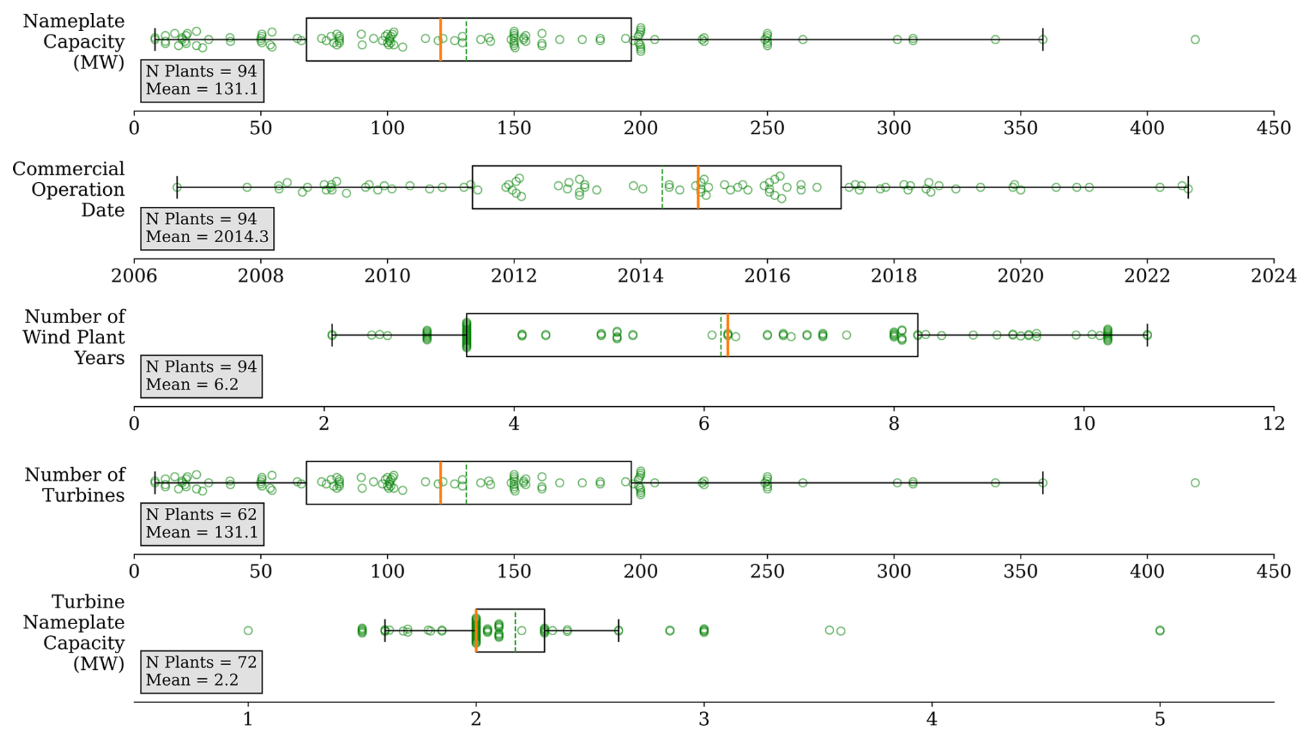
Figure 1 Summary of the key characteristics of the wind plants that have both EYA and monthly operating data. From top to bottom: the boxplots show the distribution of the project's nameplate capacity, COD, number of turbines, and turbine capacity, where that information is available in the EYA data.

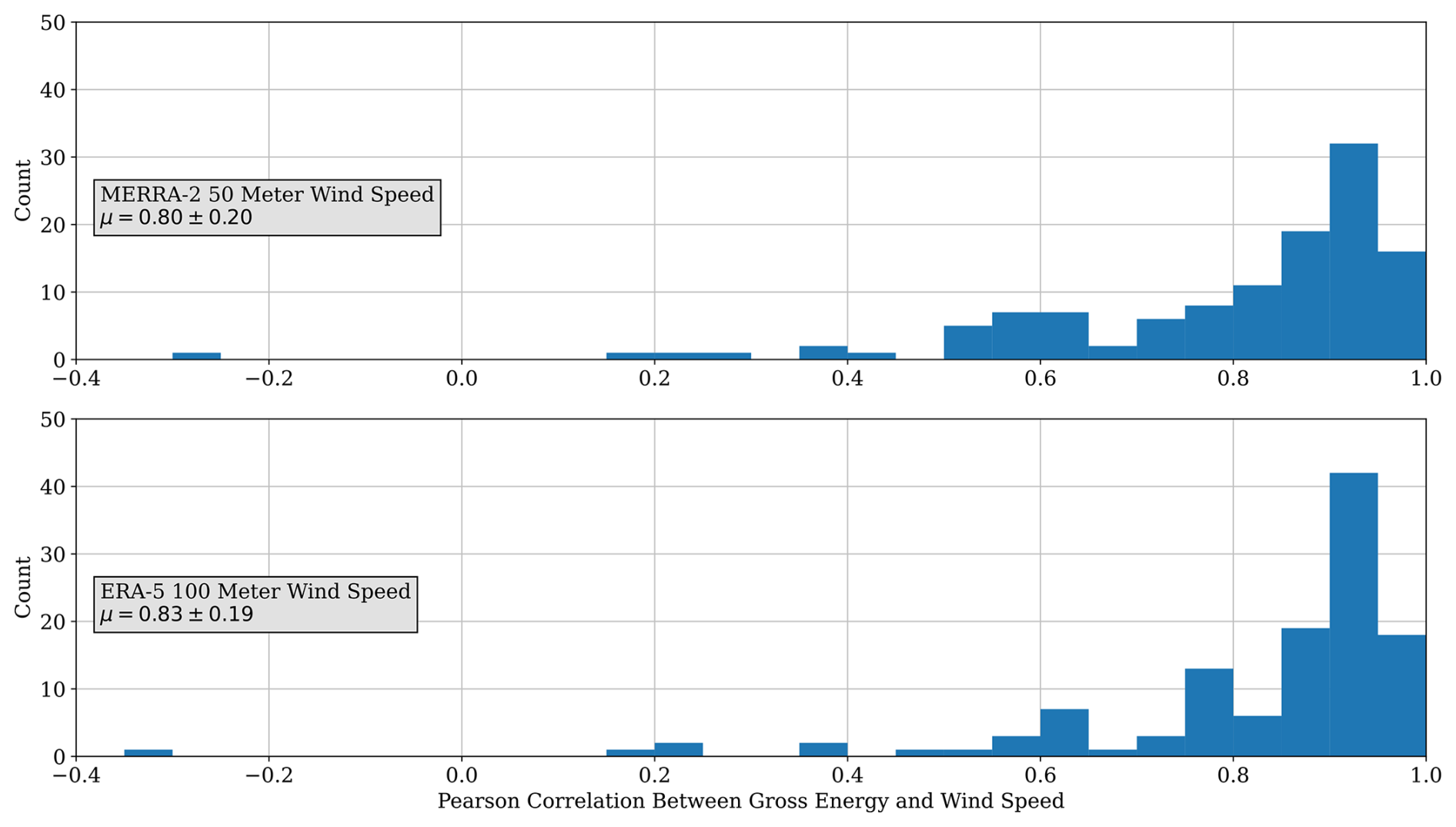
Figure 2 Histogram of the correlation between the monthly gross energy production and each of the monthly MERRA-2 50 m wind speed (top) and ERA5 100 m wind speed (bottom) for each wind plant for the nearest available coordinate.

For each wind plant, we also collected the ERA5 (Hersbach et al., 2018) and MERRA-2 (Global Modeling and Assimilation Office (GMAO), 2015) reanalysis datasets for long-term wind resource corrections. The MERRA-2 data are made available at 0.5° × 0.625° resolution, and the ERA5 data are available at 0.25° resolution, so we identified the closest latitude and longitude to each plant's owner-provided centroid and used the atmospheric data corresponding to that point. For each point, we downloaded the hourly wind speed, wind direction, temperature, humidity, and surface air pressure and aggregated these readings to the monthly mean reading for each variable. Figure 2 demonstrates the high degree of correlation between gross energy production (discussed further in Sect. 2.2) and the MERRA-2 and ERA5 wind speed data as measured by the Pearson correlation coefficient. While MERRA-2 demonstrates a higher average Pearson correlation coefficient (0.83) than the ERA5 data (0.80), their median values show a reverse trend, with ERA5 having a 0.90 median correlation and MERRA-2 having a 0.88 median correlation. The close alignment of reanalysis wind speed and gross energy suggests that for most projects, the reanalysis wind conditions are suitable for analysis.

We found that the five projects with a correlation coefficient less than 0.4 represented our most extreme outliers in the operational analysis results, so we removed them from the study. We also found that each of these projects either had upstream plants introduced following their construction, causing external wake losses, or is located in complex terrain, such as downwind from a mountainous region or among rolling hills. Further, reanalysis wind conditions were not able to fully account for complex terrain near ground level, as they are modeled from atmospheric conditions, nor could they account for every location within their coarse-grid structure. While a coarse grid means the reanalysis conditions are more or less representative of the data for that plant, there is no correlation between distance from the modeled grid point and the plant's centroid for either the poorly matched plants or the data set writ large.

2.2 Operational analysis

The first set of analyses assessed the similarities between the P50 biases using the annual net energy provided through the EIA and MORs. To annualize the energy production, we summed each consecutive 12-month period starting from the COD, excluding any partial years at the end of the time series. We then calculated the percentage difference between each annualized reading and the EYA-estimated P50.

Figure 3 Flowchart of the OpenOA Monte Carlo AEP methodology.

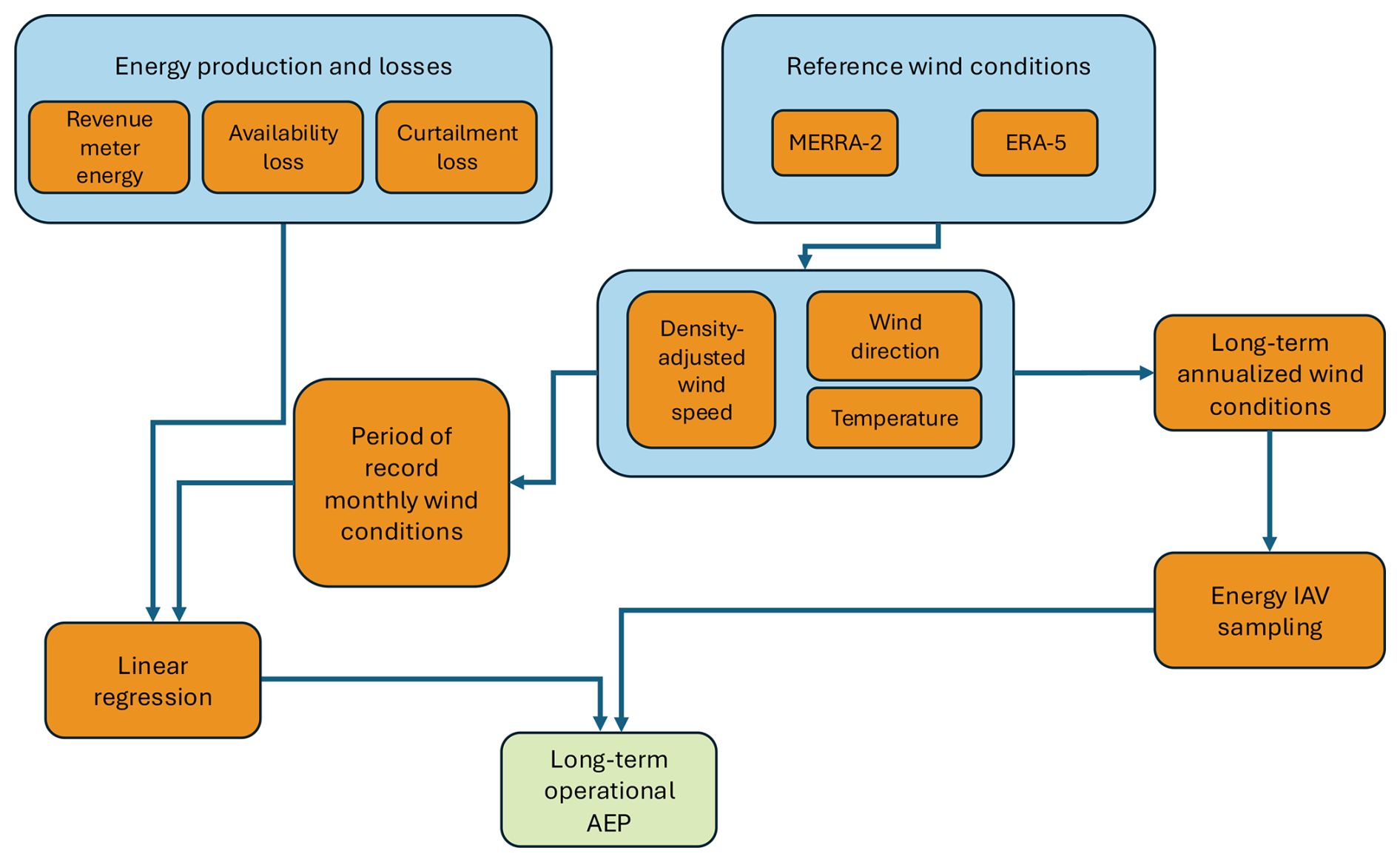
To compute the long-term-corrected P50, P90, and uncertainty estimates, we utilized the Monte Carlo AEP analysis method in the National Laboratory of the Rockies' OpenOA software (Perr-Sauer et al., 2021), as described in Bodini and Optis (2020), outlined below, and shown as a flowchart in Fig. 3. The method includes the following steps:

1. Compute the density-corrected wind speeds for each reanalysis product, and average the hourly wind speed, wind direction, and temperature to a monthly level to align with the operating data.

2. Flag months where the losses were unreported, and remove months where no energy data were available.

3. Calculate gross energy by adding the revenue meter energy, availability loss, and curtailment loss, and normalize each month to a 30 d period.

4. Run a linear regression between the gross energy production and density-corrected wind speeds, the sine and cosine components of the wind direction, and temperature.

5. Apply the linear regression to the long-term, density-corrected wind speed, wind direction, and temperature data.

6. Correct the long-term gross energy estimates, which are based on 30 d months, for the correct number of days in each month.

7. Subtract the monthly average availability losses to estimate monthly net energy.

8. For analyses comparing the 1-year uncertainty, include the interannual variability (IAV) uncertainty factor, and for analyses compared to the long-term uncertainty, exclude the IAV. The IAV uncertainty component is sampled from a normally distributed random variable, centered on the 20-year standard deviation of the energy production estimates.

The long-term correction is similar to the approach taken in Lunacek et al. (2018), with a few essential differences in the data used and how they are filtered. The reanalysis datasets were of a different vintage, and only the wind speed data were used in Lunacek et al. (2018). No curtailment or availability data are provided through the EIA, so there was no gross energy calculation, nor was a 30 d normalization applied in Lunacek et al. (2018). The outlier filtering in Lunacek et al. (2018) was based on the standard deviation from the mean, different from the more robust approach taken in this study.

For each iteration in the Monte Carlo analysis, we randomized the usage of the variables listed in the top section of Table 1. The bottom section represents variables that are varied between analyses but held constant within an analysis. Additionally, we defined what OpenOA uses as a default value, how each simulation of the Monte Carlo analysis applies that value, and what variations of the Monte Carlo analysis we ran. For the simulation's parameter choice, OpenOA randomly chooses one of the input variables, randomly samples from a normal distribution using the input value as the distribution's center or a uniform distribution with the input value acting as the lower and upper bound, or does not vary the parameter's value at all between runs. The choice for the default values was not documented when the model was originally built; however, it is expected that the uncertainty in energy losses will be higher than the net energy, as the losses are derived based on the estimated potential energy production rather than directly measured at the revenue meter. For the combined loss threshold parameter, we found that typically between 4 and 16 months will be removed from an analysis, representing as little as 9 % and as much as 28 % of the available records. Despite removing many records for some plants, this filtering significantly reduced the overall long-term-corrected uncertainty. We used the Huber loss method because it is more robust to outlier data (Huber, 1964), such as high curtailment or low-availability months, which are not representative of regular plant operations. For each combination of model configurations, we ran 5000 Monte Carlo iterations, including bootstrapping the monthly operational data and randomly sampling different analysis parameters to understand the uncertainty in the operational assessments for each plant. The rightmost column of Table 1 represents the input parameter variations that we ran to identify the analysis settings that yield the most accurate and reliable estimates.

Table 1 Description of the modeling parameters varied between individual simulations of the Monte Carlo analysis, their corresponding OpenOA default values, and how these parameters are varied between each Monte Carlo analysis.

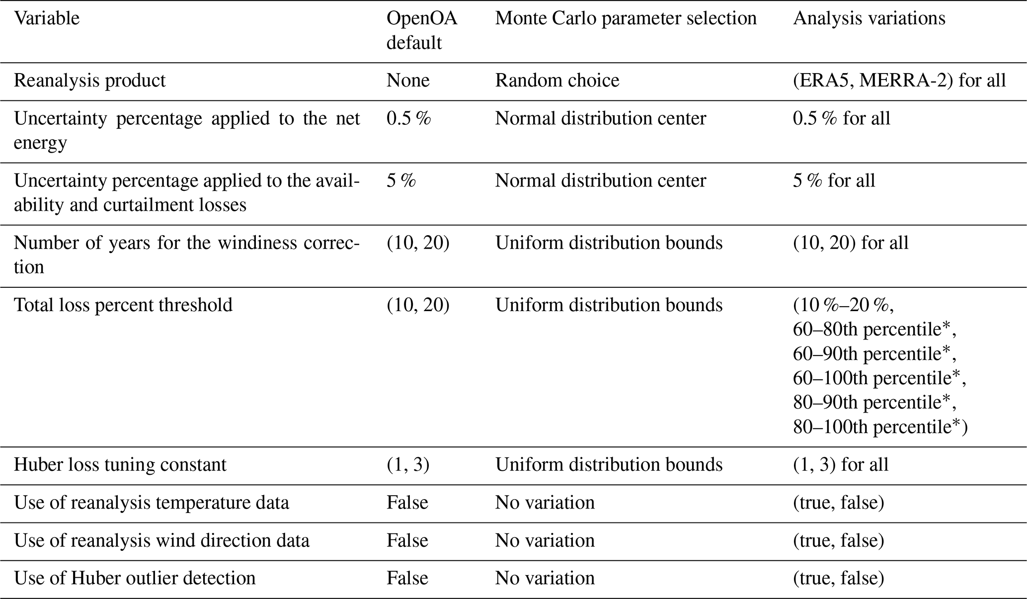
^* denotes that the listed number is a percentile, and the percentage is calculated separately for each project.

To select a representative model for each of the combinations, we chose the lowest total rank by comparing the R² of each bootstrapped model and the total uncertainty (${\mathit{\sigma }}_{\mathrm{AEP}}/{\mathit{\mu }}_{\mathrm{AEP}}$). Using each of these metrics, we summed the ranking of the lowest total uncertainty and maximum median R². We selected the lowest total rank model as the representative model for each plant, as it would have minimized uncertainty and maximized how well the model fits the test data. Using the 5000 iterations, we computed the P50, P90, and uncertainty of the AEP estimations.

When computing the results, we also gradually filtered out time periods and projects to arrive at a more accurate assessment of each wind plant and the industry more broadly. We removed the first year of operational data to account for non-representative issues that arise in the first year of operations. Then, we removed projects with a COD earlier than 2011 to account for changes in EYA methodology. Finally, we considered the combination of both filters.

3 Results

Here, we present the results of our validation of the approach taken in Lunacek et al. (2018) that formed the basis of our work and our operational analysis performed on owner-provided data. In Sect. 3.1, we compare results using the EIA-reported monthly net energy to results based on the owner-provided MOR data. In Sect. 3.2, we report on operational analysis of the MOR data to assess the bias present in EYA-estimated gross energy production and the uncertainty in the EYA estimates.

3.1 Validation of the original approach

As a first step, we confirmed the validity of the approach to rely on monthly EIA net energy data to determine AEP from the original study (Lunacek et al., 2018). This step ensures that we are able to make a reasonable comparison because there is not a specification for how the EIA data are provided by plant owners or what processing steps (if any) are performed prior to being provided to end users. To do this, we compared the EIA net energy output to the MOR net energy, where the EIA identifier was provided with the EYA data. As shown in Fig. 4, the correlation between the MOR energy production received from plant owners and operators and the energy reported by the EIA was strong (ρ=0.98). The line of best fit for the EIA and MOR data yields $y=\mathrm{0.99}x+\mathrm{0.30}$, indicating that the EIA data are highly consistent with those reported by wind plant owners. This result indicates that the methods used by Lunacek et al. (2018) to set a baseline for P50 bias remain valid overall, though significant discrepancies exist for individual months.

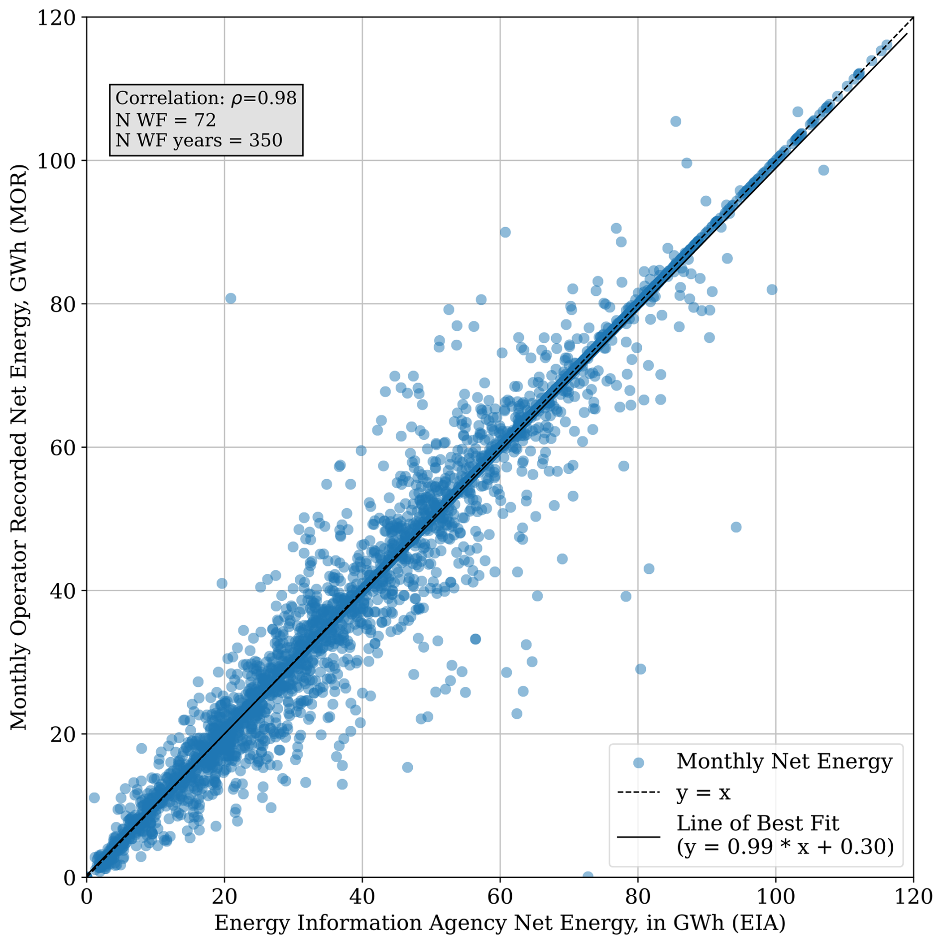
Figure 4 Relationship between EIA-reported monthly net energy and MOR net energy. The line of best fit demonstrates that the EIA net energy closely tracks that of the MORs.

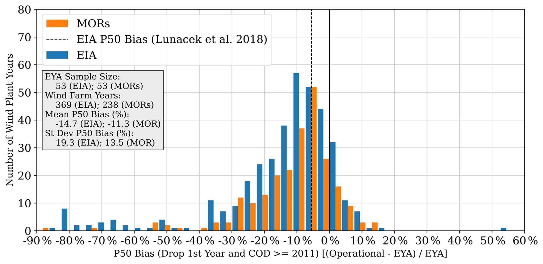
We then compared the EYA AEP P50 bias for both the net EIA energy and the net MOR energy without a long-term correction to the bias resulting from Lunacek et al. (2018), as shown in Fig. 5. We took the best-case scenario, where we removed the first operational year of the wind plant and removed plants with a COD prior to 2011. This approach is similar to the approach taken in Lunacek et al. (2018), which reported a 5.5 % overprediction when using a long-term correction. Here, the average P50 biases for the uncorrected EIA and MOR data are −14.9 % and −11.5 %, respectively. However, there is a large variation in the bias for individual plants (19.3 % for EIA data and 13.5 % for MORs), with positive biases (underprediction) for many plants. As expected with uncorrected values, there is a significant number of outliers for AEP overprediction, particularly for the EIA data, which has 55 % more wind farm years of data. In general, this finding indicates that there is still an overprediction of AEP P50 in the EYAs, given that it is at least double the long-term-corrected value reported in Lunacek et al. (2018).

Figure 5 Comparison of the P50 bias between the EIA net energy and MOR net energy.

3.2 Long-term-corrected results

The next phase of the analysis was to estimate the long-term-corrected AEP and uncertainty. As described in Sect. 2.2, we found each project's ideal analysis settings; we report on the long-term-corrected results in this section. We found that 84 % of the best combinations included the use of the Huber loss algorithm outlier detection and filtering, 74 % used the reanalysis temperature data, and 33 % used the reanalysis wind direction. For the uncertainty loss thresholds, we found that 21 % of the best combinations used the OpenOA default value, and another 46 % used thresholds with a minimum of the 80th percentile. Combined, 47 % of the best model combinations also used the outlier detection and temperature data but no wind direction data.

In Fig. 6, we demonstrate the overall long-term-corrected P50 bias by COD where there is modest yet inconsistent improvement in the P50 bias between 2011 and 2019 relative to projects prior to 2011. However, in 2019 and later, the P50 bias worsens, though it is worth noting that there are fewer projects and therefore less operational data in our dataset in this COD grouping, so the results may not be representative. Even with later COD P50 bias increases, the post-2010 COD wind plants exhibit an improving P50 bias, −7.4 % vs. −6.6 %, as shown in the text box of Fig. 6, which is in line with the baseline result trends from Lunacek et al. (2018). To further test whether or not there is a relationship between CODs prior to 2011, we ran a two-sided Welch's t test (Welch, 1947) for years prior to 2011, 2011 through 2022, and 2011 through 2019 to account for the effect of small sample sizes in projects coming online later against the P50 bias of all samples and those dropping the first year of operational data. For all combinations, a p value greater than 0.2 was yielded, demonstrating that there is not a strong relationship between the EYA estimation methods prior to 2011 and those used starting in 2011.

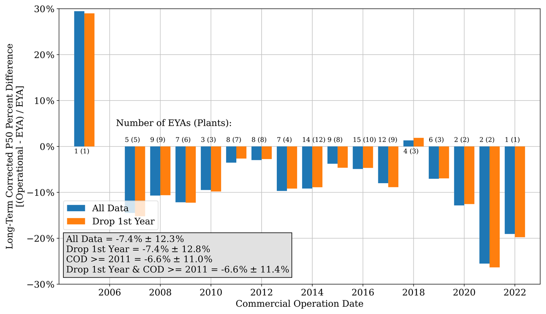
Figure 6 Histogram of the P50 bias by COD for all projects and for all projects when removing their first year of operations.

We similarly found that there was a possibility of a relationship between states, provinces, or small countries with at least four plants and their long-term-corrected P50 bias. In Fig. 7, it can be seen that states such as Oklahoma, New Mexico, Nebraska, and New York tend to have above-average P50 biases compared to some states like Texas and California that have many below-average P50 biases. When running a one-way ANOVA (Welch, 1951), we found a p value of 0.003, so we ran Tukey's test (Tukey, 1949) against the pairs, only finding a significant difference between California and Oklahoma (p value 0.03) and California and New Mexico (p value 0.019). However, when we ran a one-way ANOVA (Welch, 1951) to further inspect the relationship between original equipment manufacturers (OEMs) and long-term-corrected P50 bias, we found no relationship, with a p value of 0.043 for OEMs with at least four data points. For other key distinguishing variables, there were not enough data available relative to the total plants analyzed to warrant further testing.

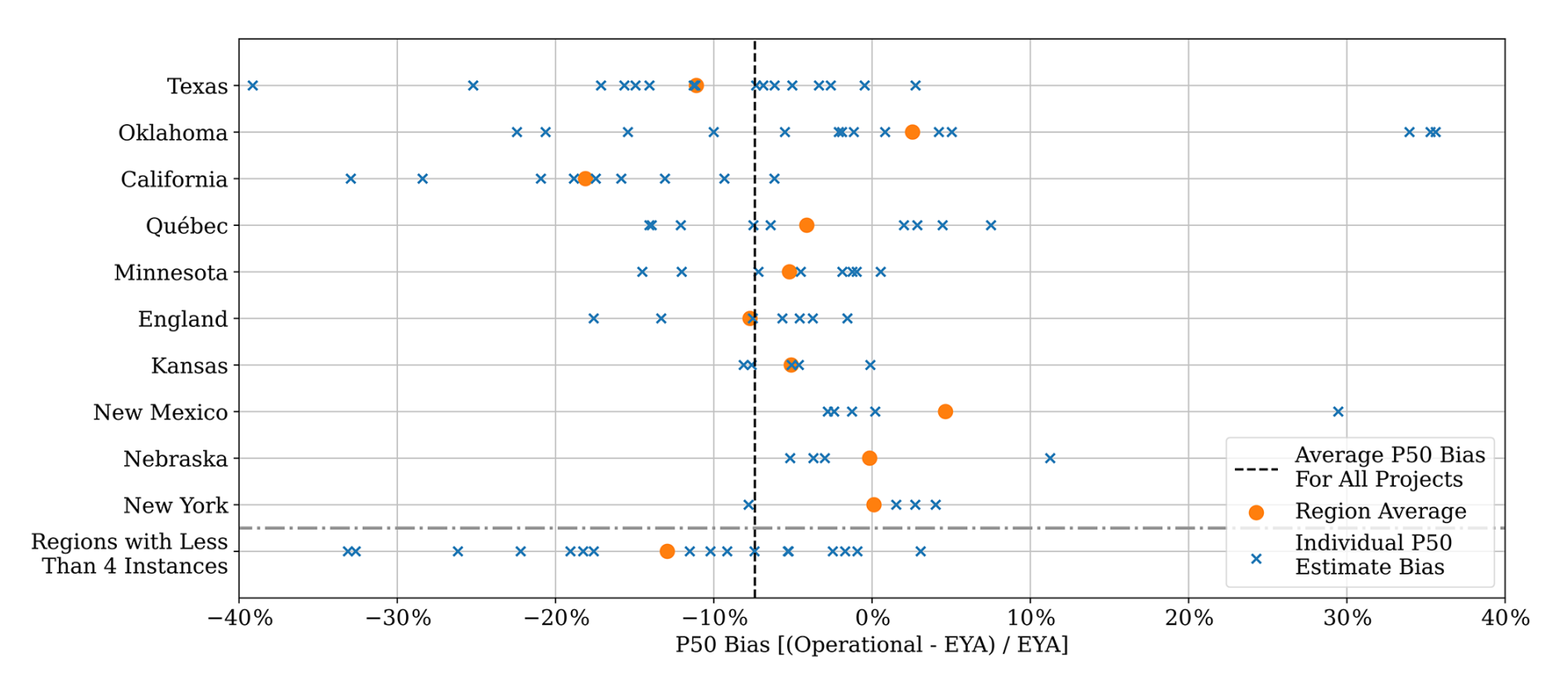
Figure 7 Scatter plot of each state, province, or country's individual P50 estimate biases and P50 estimate biases for regions with small sample sizes.

We also demonstrate the P50 bias for each consultant in Fig. 8 to determine if there were any significant variations across the 19 consultants. Most deviation from the average P50 bias occurred in consultants with a small sample size or where the spread was large. In particular, consultants 1, 3, 6, and 8 had a large spread in their individual estimates; only consultant 5 demonstrated a high level of precision in their estimates. The unspecified grouping, corresponding to no consultant name being provided, yielded the largest sample size with some of the smallest spread in EYA P50 bias. Nevertheless, when performing a one-way ANOVA test for all consultants with at least three data points, we found a p value of 0.7263, confirming there is no meaningful difference between consultant predictions of P50 energy production.

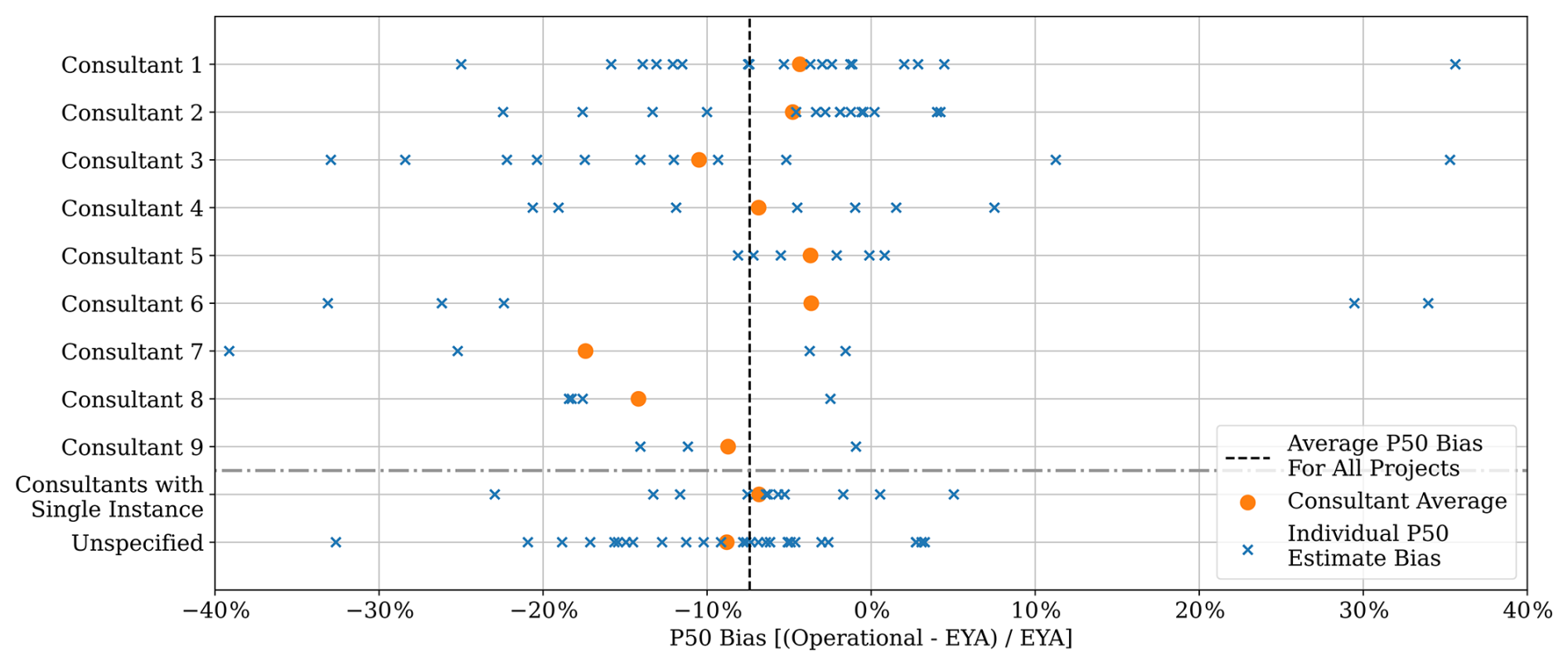
Figure 8 Scatter plot of each consultant's individual P50 estimate biases and P50 estimate biases without a specified consultant.

Using the 5000 simulations, we then computed the P50 and P90 as their respective 50th and 10th percentiles and the uncertainty as ${\mathit{\sigma }}_{\mathrm{AEP}}/{\mathit{\mu }}_{\mathrm{AEP}}$. The boxplots in Figs. 9, 10, and 11 demonstrate the distribution of the per-project spread of the P50, long-term P90, and long-term uncertainty bias, respectively, for each of our four down-selection criteria. Compared to the Lunacek et al. (2018) results, we can see a slightly worsening P50 bias. We observe that the short-term P90 bias is positive, indicating that the P90 of the estimated operational AEP exceeds the EYA AEP P90 value on average. However, this result does not necessarily suggest that the EYAs use overly conservative means for estimating high-probability energy production levels; to reach this conclusion, we would need to demonstrate that the estimated operational AEP exceeds the EYA P90 predictions 90 % of the time.

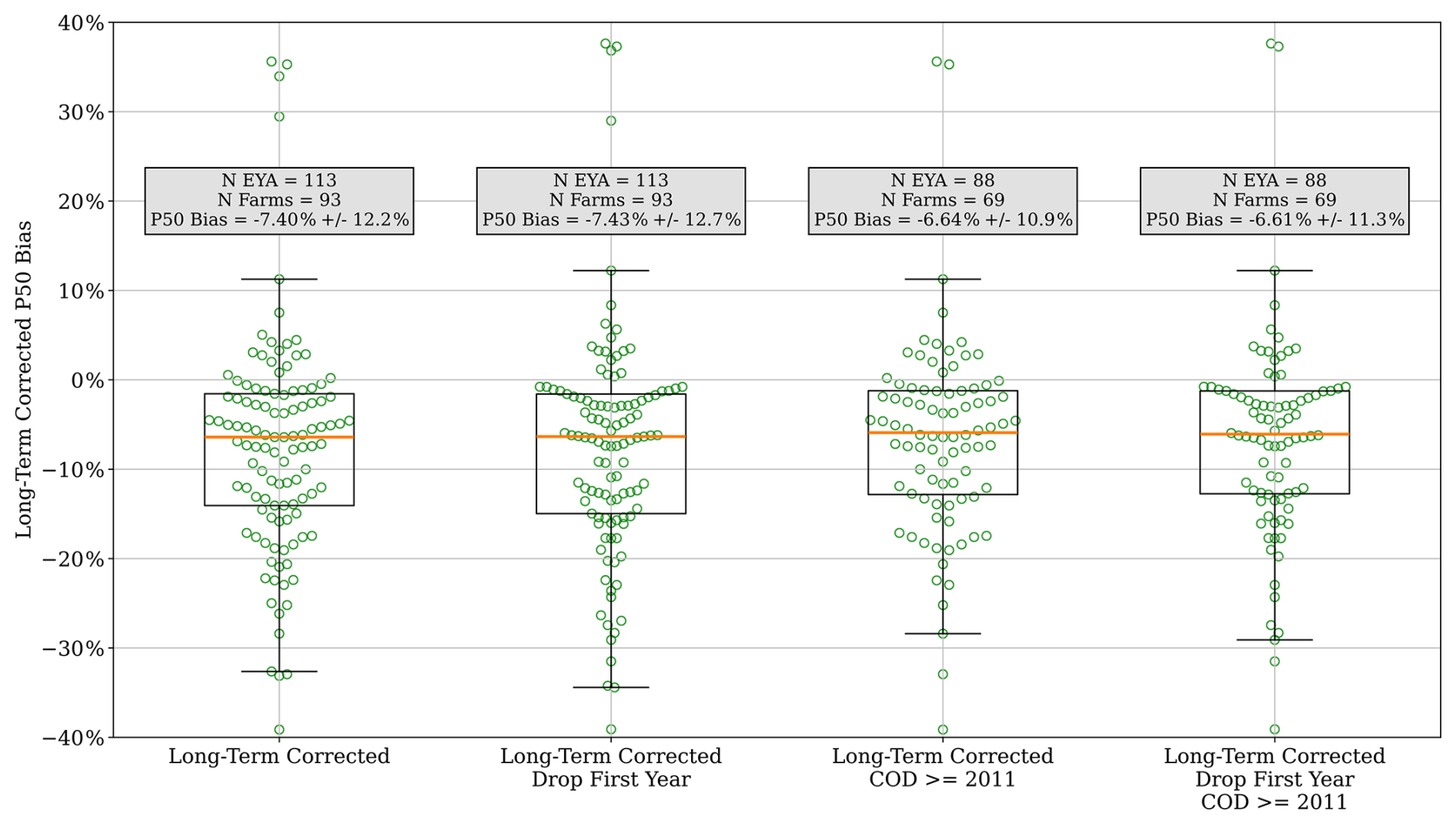
Figure 9 Boxplot showing the project-level P50 bias for each of the project down-selection criteria.

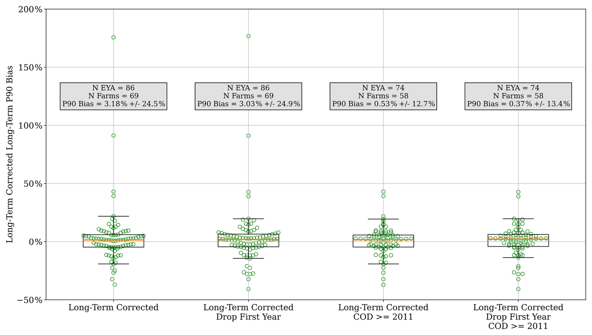
Figure 10 Boxplot showing the project-level long-term P90 bias for each of the project down-selection criteria.

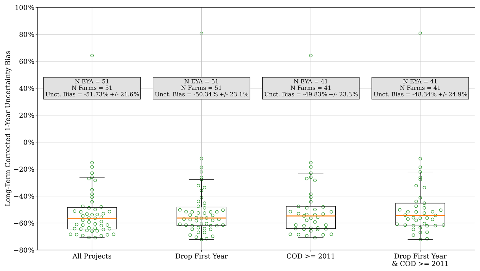
Figure 11 Boxplot showing the project-level long-term-corrected uncertainty biases relative to their 1-year EYA uncertainty estimate for each of the project down-selection criteria.

As indicated, the uncertainty bias for the long-term-corrected energy estimates relative to the 1-year EYA uncertainties appears to suggest that the EYAs are routinely conservative estimates of uncertainty, with the average bias in the −52 % to −48 % range. It should be noted, though, that the uncertainties for the operational AEP estimates and the EYA AEP predictions are not defined equivalently. The operational AEP uncertainties represent the uncertainty in the long-term AEP based on realized energy production during an initial period of operation. EYA estimates, on the other hand, represent the uncertainty in the predicted AEP before the plant is built. The EYA estimates are expected to have a higher degree of uncertainty because there are a significant number of individual model uncertainties and potential sources of loss to consider when predicting energy production prior to building a wind plant.

To better understand the uncertainty and prediction errors, we also computed the prediction error of the EYA P50 and P90 estimates for each plant relative to each Monte Carlo iteration's AEP estimation for the corresponding plant (percentage difference between the EYA reading and each iteration's AEP estimate), as shown in Figs. 12–14. In Fig. 12, which shows the distribution of P50 prediction errors including IAV, we smooth the error histogram to highlight the centering around the mean values. Importantly, we found that the standard deviation of the sample errors ranged from 11.9 % to 13.7 %, which closely aligns with the average 1-year uncertainty in the corresponding EYAs of 10.5 %±2.6 %, shown on the right side of Fig. 12. However, when comparing the EYA long-term uncertainty to the P50 prediction errors that exclude IAV, as shown in Fig. 13, our standard deviation ranges from 11.4 % to 13.1 %, which is much larger than the corresponding EYA long-term uncertainties of 7.5 %±2.1 %. As opposed to the direct comparison in Fig. 11, these results indicate that the EYA uncertainty, especially the long-term uncertainty, is being underestimated.

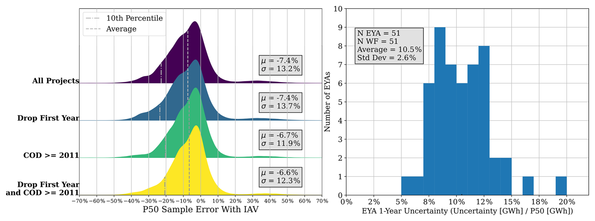
Figure 12 (left) Ridge plot showing the percentage error of each sample's AEP value calculated with IAV relative to EYA P50. (right) Histogram of the EYA 1-year uncertainty values.

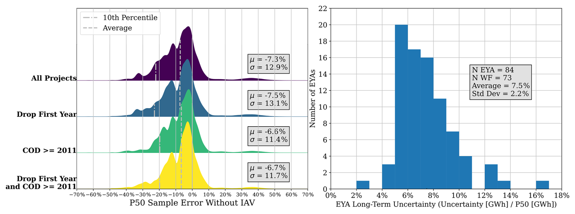
Figure 13 (left) Ridge plot showing the percentage error of each sample's AEP value calculated without IAV relative to EYA P50. (right) Histogram of the EYA long-term uncertainty values.

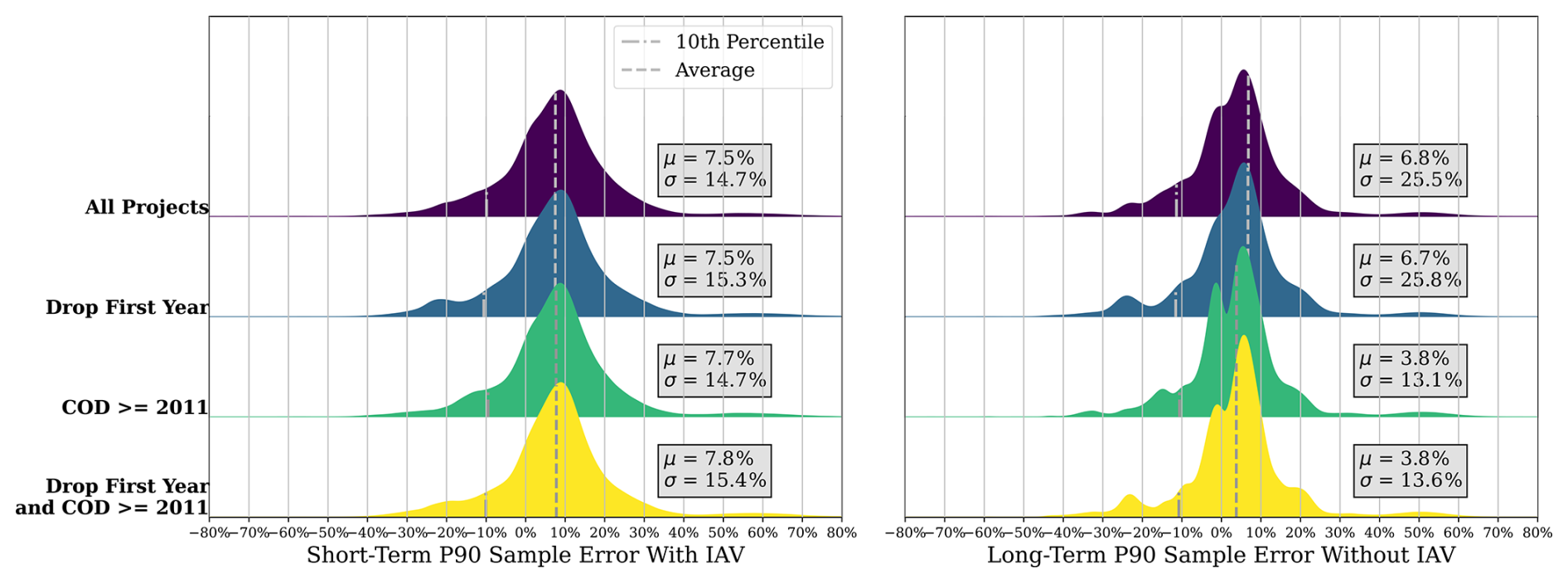
Figure 14 Ridge plots showing the percentage error of each sample's AEP value relative to the EYA P90. (left) The comparison is made between the analyses run with IAV and the EYA short-term P90. (right) The comparison is made between the analyses run without IAV and the EYA long-term P90.

In line with our project-level P90 estimate comparisons (though more positive), the individual P90 prediction errors for each Monte Carlo iteration center around positive values (Fig. 14); however, the 10th percentile of the prediction errors is roughly −10 % for all cases, demonstrating that EYA P90 estimates are not conservative enough for both the 1-year and the long-term P90 predictions. Ideally, the 10th percentile should be 0 %, meaning the realized operational AEP exceeds the EYA P90 predictions at least 90 % of the time. Note that we can still see the impact of outlier data in the spread of the distribution and the presence of additional peaks.

Considering the continued existence of EYA P50 bias, we then calculated the true probability of exceedance value (PXX value) of the EYA-reported P50 based on the long-term-corrected distribution and the PXX value of the long-term-corrected P50 with respect to the EYA distribution statistics. We derived the respective PXX values by first finding the number of standard deviations by which the estimated P50 value was from the comparative mean, $x=(\mathrm{P}{\mathrm{50}}_{\mathrm{ltc}}-{\mathit{\mu }}_{\mathrm{eya}})/{\mathit{\sigma }}_{\mathrm{eya}}$. Then, we calculated the probability based on the cumulative distribution function of the number of standard deviations and subtracted it from 1 to ensure the overestimates yield a lower PXX value than the P50. We followed the same process for the long-term-corrected P50 with respect to the EYA AEP distribution by computing the number of standard deviations ($x=(\mathrm{P}{\mathrm{50}}_{\mathrm{eya}}-{\mathit{\mu }}_{\mathrm{ltc}})/{\mathit{\sigma }}_{\mathrm{ltc}}$), calculating the probability from the cumulative distribution function, and subtracting it from 1 to account for the overprediction bias. The results of these calculations for all plants are shown in Fig. 15. We found that the EYA P50 represented a P22 on average, with a standard deviation of 30 percentage points, and that the long-term-corrected P50 represented a P72 with respect to the EYA AEP distribution, with a standard deviation of 26 percentage points. The two distributions roughly mirror each other and form clusters, where the EYA P50 is significantly overestimated. For the long-term-corrected distribution, the EYA P50 is −0.95 ± 1.61 standard deviations from the long-term-corrected mean, with the bottom 25 % of the distribution being at most −1.64 standard deviations. Similarly, the long-term-corrected P50 is on average 2.16 ± 2.84 standard deviations from the mean EYA-estimated AEP, with the top 75 % of the data being at least 3.99 standard deviations from the mean. Table 2 shows that when comparing the subset of plants with CODs after 2010 and when removing the first year of operational data, the results improve slightly. For example, the EYA P50 PXX value relative to the long-term-corrected distribution corresponds to a P24 compared to a P22 when viewing all plants with all available operational years. Similarly, the long-term-corrected P50 based on the EYA distribution shifts from a P72 to a P70 when filtering out plants with CODs prior to 2011 and removing the first year of data.

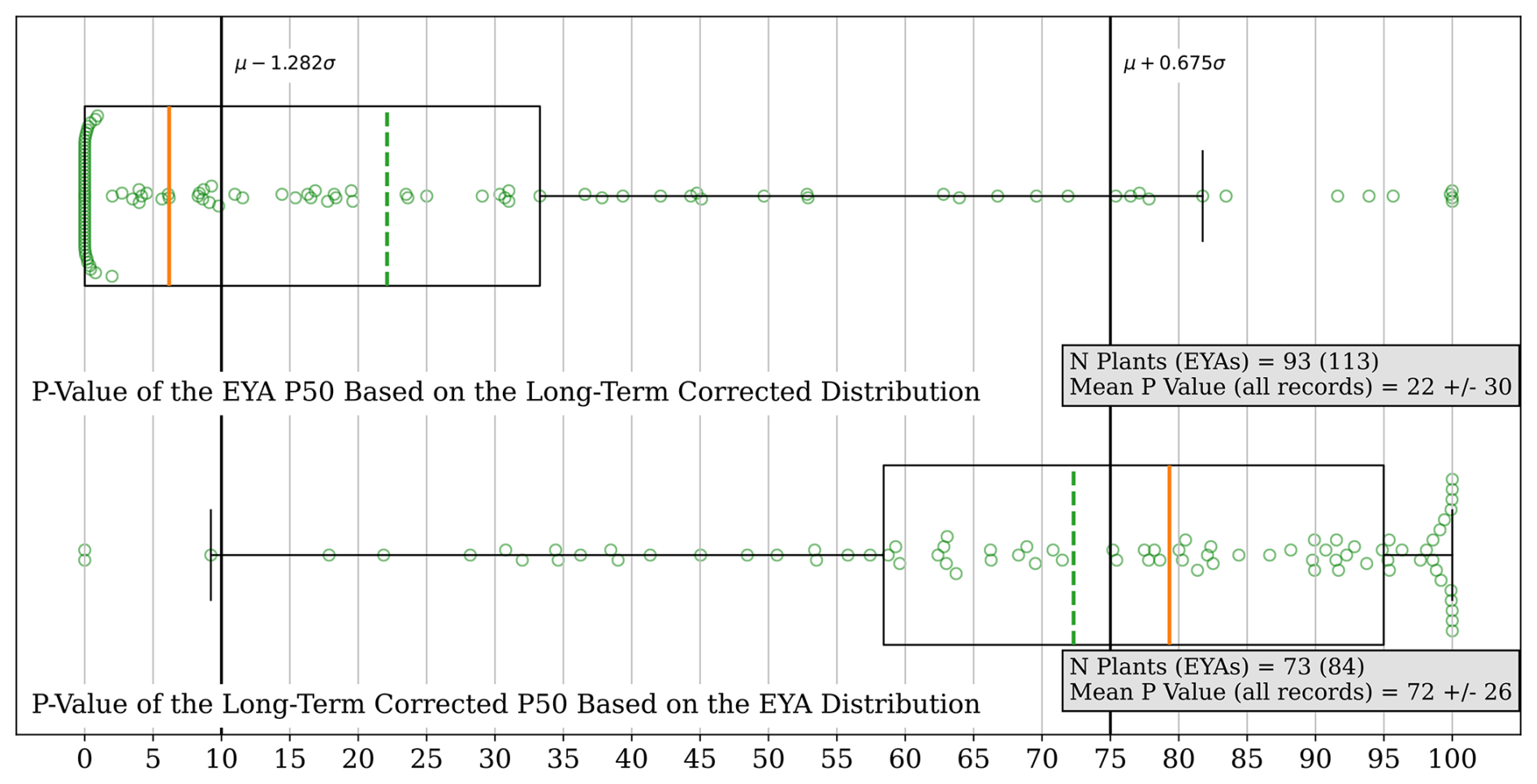
Figure 15 Box and swarm plots for the estimation of the true PXX value of the EYA P50 based on the long-term-corrected distributions of energy generation (top) and the derived PXX value of the long-term-corrected P50 from the EYA-estimated energy production distribution (bottom).

Table 2 Table of the EYA P50 PXX value based on the long-term-corrected distribution and the long-term-corrected P50 PXX value for each of the data subsets.

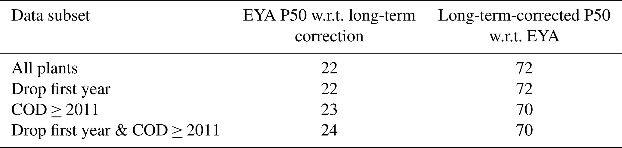
Table 3 Table of the EYA P50 and EYA P90 PXX values based on the long-term-corrected prediction error for both the short-term (with IAV) and the long-term (without IAV) distributions.

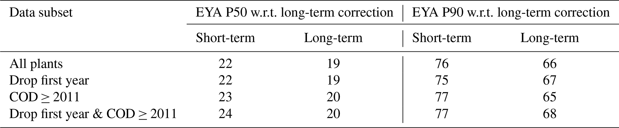
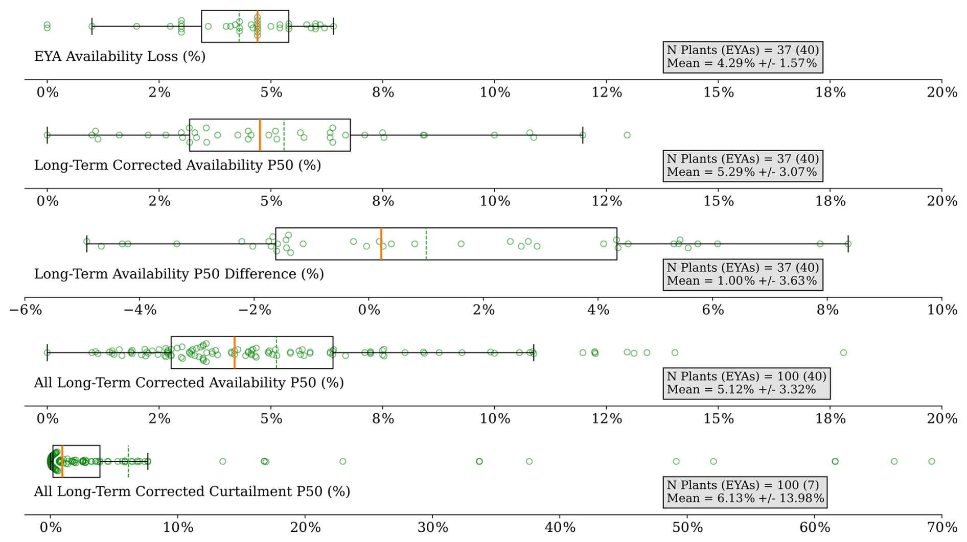
Figure 16 Summary of the EYA-estimated availability losses (mixture of time and energy based), long-term-corrected P50 of operational availability and curtailment losses, and the percentage point difference between the operational availability P50 and EYA availability losses. From top to bottom: the boxplots show the distribution of EYA availability loss, the long-term-corrected operational availability loss P50, the difference between the long-term-corrected operational P50 and EYA-estimated availability losses, the long-term-corrected operational availability loss P50 for all projects, and the long-term-corrected operational curtailment loss P50 for all projects.

Another way to understand what the P50 and P90 values represent based on the long-term-corrected distribution is to compute what percentage of the P50 and P90 prediction errors (as shown in Figs. 12–14) is greater than 0 %. In Table 3 we demonstrate the close alignment these prediction error results have with those presented in Fig. 15 and Table 2. The EYA P50 corresponds to a P19 to P20 based on the long-term-corrected AEP distributions without IAV, depending on the scenario, and the long-term EYA P90 corresponds to a P65 to P69, depending on the scenario. For both the short-term P50 and the P90, the PXX values improved with the long-term-corrected AEP distributions, with IAV yielding a realized P22 to P24 for the EYA P50 value and a P75 to P77 for the EYA 1-year P90 value, depending on the scenario.

Finally, because EYA availability and curtailment loss estimates were provided for 36 projects, we also computed the P50 value for each of the long-term-estimated operational availability and curtailment losses in the Monte Carlo simulations by project, as shown in Fig. 16. We have excluded a detailed comparison between the EYA-estimated curtailment losses and operational curtailment losses, as 31 of the EYAs provided an EYA-estimated 0 % curtailment loss, and only two EYAs estimated 0 % availability losses, which were removed from the comparison. As such, the results of the availability comparison are shown in Fig. 16. We found that the average difference between the operational P50 values and EYA estimates for availability losses was 1 percentage point, indicating a slight underestimation of availability loss; however, the median value is 0.22 percentage points, and the standard deviation is 3.63 percentage points. Taken together, this suggests an inconsistent understanding of availability across the board, even if it contributes a minimal amount to the AEP P50 biases. Further, it should be noted that availability data were provided in mixed formats – energy lost and time-based availability – so the comparisons are not wholly on the same basis.

The curtailment P50 bias only consists of seven comparisons, so the underestimation of losses by 13 ± 23 percentage points may not be representative of reality. In fact, many of the EYAs with curtailment loss information state outright that situations where the energy grid may force the power plant to stop sending power are not considered, so the comparison of realized curtailment and EYA-estimated curtailment likely provides little insight without further details or delineations.

4 Conclusions

In this paper, we built on the methodology of the work performed in Lunacek et al. (2018) by gathering operational data from wind plant owners and operators that include the curtailment and availability losses that could not be accurately accounted for in the original work. We observed many of the same relationships as the original study, such as an overprediction of energy yield from consultants and a shrinking P50 bias following the change in methodology in 2011. However, we found that P50 bias has remained in line with but is slightly worse than (0.8 % to 1.1 % higher) Lunacek et al. (2018), now that we include more recent projects and are able to account for curtailment and availability losses. Additionally, we observed that the EYA uncertainty and P90 estimates are not conservative enough when compared to the observed distributions of AEP prediction errors relative to the operational AEP estimates, although the EYA 1-year AEP uncertainties are a reasonable approximation of the observed uncertainty.

This work motivates additional research to understand how the EYA process can be improved to reduce the AEP P50 overprediction bias and better characterize the uncertainty in the predictions, especially because P50 bias appears to be increasing compared to the findings in Lunacek et al. (2018). Our results ultimately raise further questions that were out of the scope of this study. One example is to measure the impacts of external wakes from neighboring farms that came online after a plant's EYA was completed, and the extent to which they contribute to P50 overprediction bias. Many projects represented in this dataset are older, and it is likely that neighboring projects have been built since their inception, creating unaccounted-for losses in the EYAs that would be present in the MORs.

A more fundamental question would be whether working with higher-resolution operational data, turbine operating status, and consistently delineated loss data combined with more advanced long-term operational AEP modeling could provide a more accurate or less uncertain long-term correction. As in Lunacek et al. (2018), it remains an open question of how to curate a broader selection of wind plant MORs, EYAs, and plant characteristics to understand the effects that plant characteristics such as geography or turbine technology can have on energy production.