Introduction of the virtual center of wind pressure for correlating large-scale turbulent structures and wind turbine loads

For modern wind turbines, the effects of inflow wind fluctuations on loads are becoming increasingly critical. Using field measurements of a full-scale operating wind turbine and simulated loads calculated with reconstructed wind fields from wind measurements from the GROWIAN campaign, we identify particular load events that lead to high values of the so-called damage equivalent loads. Remarkably, the simulations do not reproduce such load occurrences when standard synthetic turbulent wind fields are used as inflow. These standard wind fields are typically parameterized by statistics at a single measurement location (e.g., mean wind speed and turbulence intensity). In this article, we introduce a new characteristic of a wind field: the virtual center of wind pressure. The new feature is calculated from averages of the dynamic pressure on a defined area, i.e., the rotor disk. We correlate these characteristics to the unusual load events observed in the operational measured data. Furthermore, we demonstrate that the introduced concept is an efficient tool to characterize large-scale structures within wind fields. We propose using the virtual center of wind pressure in conjunction with the well-defined single-location properties to consolidate improved descriptions of atmospheric wind and more accurate wind fields for turbine simulations.

1 Introduction

The correct estimation of operational loads is of central importance for the design and certification of wind turbines. Current challenges and recent developments in wind energy have led to larger-sized and more slender turbines (Veers et al., 2019, 2023). As a result, the loads estimated with standard tools used for previous (i.e., smaller and stiffer) turbine designs are less and less comparable to measured loads. In particular, the accurate determination of loads caused by turbulent inflow conditions is a significant challenge due to not-yet-investigated interactions between larger elements of the turbine (i.e., turbine blades) and larger scales and heights of atmospheric wind structures (van Kuik et al., 2016; Veers et al., 2019).

To cover the broad range of operating scenarios over the lifetime of a wind turbine, atmospheric conditions are usually specified by the International Electrotechnical Commission (IEC) guidelines (IEC, 2019). According to the IEC standard, turbulent wind fields are generated using the Kaimal (Kaimal et al., 1972) or Mann (Mann, 1998) models. These models are parameterized by simple statistical quantities, e.g., mean wind speed and shear, turbulence intensity, and integral or coherence length scales. Here, simplified assumptions are made to describe the coherence of the wind field over a plane perpendicular to the main direction (Davenport, 1961; Thedin et al., 2022). The decrease in correlation with distance is typically assumed to be an exponential function. Moreover, extrapolations using power or logarithmic laws assume a change in wind speed with height in the so-called wind profiles. The exponents that parameterize these laws are typically fixed for a given location. However, analyses of wind measurements have proven the high variability of such velocity profiles, with even negative gradients (Gualtieri, 2016; Wagner et al., 2011). Moreover, wind profiles are calculated based on 10 min averages over height. Consequently, wind gradients on scales below 10 min and multiple gradients co-occurring at different horizontal locations at the plane are unresolved. Furthermore, standard wind models do not account for extreme operating conditions, e.g., wind gusts and extreme shear. Therefore, extreme events are separately added by the IEC guideline. Particularly for wind gusts, the isolated event is assumed to have a Gaussian temporal evolution and be coherent over the whole rotor plane. However, asymmetry and non-Gaussianity have been demonstrated (Hu et al., 2018). Consequently, modifications of such Gaussian and coherent assumptions have been proposed by Bierbooms and Veldkamp (2024) for improving the validity of the IEC models.

Within the wind industry, the blade element momentum (BEM) method (Glauert, 1935) is the prevalent approach for the simulation of loads. A full-scale wind turbine model is exposed to turbulent inflow within the BEM simulation with defined characteristics. Ideally, the loads calculated using these aero-servo-elastic simulations should accurately reproduce the loads experienced by operating wind turbines, at least statistically. This implies that the range and distribution of the simulated loads for specific inflow conditions should align with measurements obtained during comparable operating circumstances. However, this alignment is not always achieved. Turbine manufacturers and operators report discrepancies of the loads between simulations and measurements. One possible explanation for these dissimilarities might be attributed to inaccuracies within the wind fields used for the numerical estimations. Unpredicted loads at operating turbines may be induced by structures occurring in the atmosphere that have not been adequately included in the current models for generating synthetic wind fields within the IEC guidelines. Recently, different extensions of IEC wind field models have been suggested, focusing on empirically measured large-scale anisotropies in the marine boundary layer (Syed and Mann, 2024) and small-scale extremes (Friedrich et al., 2021, 2022; Yassin et al., 2023).

In this article, we introduce a new characteristic of the wind field termed the virtual center of wind pressure (CoWP), which demonstrates clear correlations to particular loads at the wind turbine. This concept offers two primary contributions. Firstly, it extends the current standard characterization of wind fields. Secondly, it proposes a potential tool for load estimations. The concept of the virtual center of wind pressure is based on the notion of the center of pressure widely used in fluid mechanics (Anderson, 1991). This quantity indicates the point-wise location of a theoretical aggregated version of the pressure field acting on a body. In comparison to standard aggregated values in the wind energy context, such as the rotor-equivalent wind speed (Wagner, 2010), which is solely a function of vertical displacement, the CoWP also accounts for horizontal “excursions” of the wind field in the rotor plane. It should be noted that rotor-equivalent and sector-averaged wind speeds have mainly been employed in the context of power output and load surrogate modeling for control purposes (Guilloré et al., 2024; Coquelet et al., 2024). Nonetheless, a clear association with the occurrence of particular turbine loads remains to be established. As will be demonstrated throughout this paper, the dynamics of the CoWP are strongly correlated with the dynamics of tilt moments determined from BEM simulations of the corresponding wind field. It can thus be used as a rough estimation method of potential load characteristics directly aggregated from the wind field. For the definition and validation of the concept, three different data sets are investigated: first, wind and load measurements from a full-scale operating wind turbine; second, wind data measured by the met mast array of the GROWIAN campaign (Koerber et al., 1988; Günther and Hennemuth, 1998); and, third, IEC standard synthetic wind fields with their corresponding BEM-estimated loads.

The paper is organized as follows. Section 2 introduces relevant definitions and methods and describes the data. In Sect. 3, the motivation for the study is outlined, with the discrepancies between simulations and measurements being demonstrated. Next, in Sect. 4, we investigate the cause of these differences. The main contribution of this paper is presented in Sect. 5 with the introduction of the virtual center of wind pressure and its correlation to loads at the wind turbine. Finally, in Sect. 6, we present the findings of our investigation and include some remarks on potential future work.

2 Definitions, methods, and data

In this section, we introduce the damage equivalent load, a well-known load estimator relevant to our analysis. Moreover, we provide a short description of the numerical method for the load estimations and details of the data to be used as the basis of our work.

2.1 Damage equivalent loads

A common criterion in the wind industry to predict the service life of the mechanical components of turbines is the so-called damage equivalent load (DEL) approach (IEC, 2019; Sutherland, 1999). The DEL is a scalar quantity that quantifies the damage induced by a one-dimensional load over a certain time span. By definition, it is a weighted sum of the amplitudes s_i of the hysteresis cycles, where each amplitude is weighted with an exponent m. The DEL is then calculated as

$$\begin{array}{}\text{(1)}& {\displaystyle }\text{DEL}={\left({\displaystyle \frac{{\sum }_{i=\mathrm{1}}^n{n}_i{s}_i^m}{n_{\mathrm{ref}}}}\right)}^{\frac{\mathrm{1}}{m}},\end{array}$$

where n_i is the number of cycles with amplitude s_i. The parameter n_ref is a reference or equivalent number of cycles, given a frequency and a period (e.g., n_ref=600 for a load time series measured over 600 s at 1 Hz ). The exponent m, known as the Wöhler exponent, is characteristic of the material and is estimated from the so-called S–N curves (Orowan, 1939). Values of m≈4 are used for welded materials, e.g., the tower or bearings, while m>10 is typical for fiberglass composite materials, e.g., the blades. According to Eq. (1), the larger the value of m, the more dominant the largest amplitudes s_i are in calculating the DEL. More details on the DEL method and the Wöhler exponents can be found in Sutherland (1999) and Minner (1945). A comparison of the DELs between simulated and measured loads is discussed in Sect. 3.

2.2 BEM aeroelastic simulations

In this study, we use the aero-servo-elastic simulation tool alaska/Wind (Institute for Mechanical and Industrial Engineering Chemnitz, 2023), which is based on a general-purpose multibody dynamics modeling system. The comparability of alaska/Wind to other state-of-the-art aeroelastic simulation tools was demonstrated in Zierath et al. (2016) and Hach et al. (2020).

To cover geometrical nonlinearities, structural blade models are represented directly by finite beam elements (Schubert et al., 2017). A Beddoes–Leishman-like dynamic stall model covers the unsteady aerodynamics, whereas a dynamic flex wake model (Hansen, 2008) covers the wake effects.

Further degrees of freedom used in the turbine model are the drive train, which incorporates a radial degree of freedom to account for flexibility, and a torsional degree of freedom modeling the gearbox. The yaw drive contains a nodding degree of freedom. The tower is modeled by a linearized flexible body containing side–side, fore–aft, and torsional degrees of freedom. The foundation is connected to the soil by soil springs. A generalized-alpha method is used to solve the system of equations of motion. A formulation is used that is particularly suitable for nonlinear equations of motion and large rotations (Brüls et al., 2012).

2.3 Wind and load data

The three data sets investigated in this work are now described:

• i.

  The first data set corresponds to operational data provided by Nordex Energy. A total of 10 min measurements of both loads of the full-scale operating Nordex turbine and wind speed data from a met mast at the turbine's location are provided. The hub of the turbine is located at 125 m, and the rotor diameter is 149 m. Wind measurements with a sampling frequency of 1 Hz at three different heights are available: at hub height at 125 m, at the lowest passage of the blade tip at 50 m, and at a height in between at 88 m.

  The operational load measurements to be investigated were selected by the manufacturer. The aim was to collect data spanning a wide range of wind conditions, i.e., mean wind speed and turbulence intensity, with enough occurrences of specific load events, which are discussed in Sect. 3. The load measurements have a frequency of 50 Hz. Due to confidentiality, the measured loads are normalized by a scaling factor.

  The distance between the met mast and the turbine, as well as the wind direction, was taken into account for the selection. Only time series were selected that lay within a specified cone around the exact wind direction from the mast to the turbine. Time offsets between the measured wind and loads were taken into account based on the distance to the mast and the mean wind speed.

• ii.

  The second data set corresponds to synthetic wind data and the resulting loads calculated through BEM simulations. Synthetic turbulent wind fields are generated by the IEC standard Kaimal wind model (Kaimal et al., 1972), which is included in the software alaska/Wind (Institute for Mechanical and Industrial Engineering Chemnitz, 2023), and by the Mann wind model (Mann, 1998), where the implementation from Liew et al. (2023) was used. We used the target spectrum method, see Liew and Larsen (2022), to set up the desired turbulence intensity in the Mann fields. The turbulence grid used covers an area of 200 m × 300 m and comprises 21 × 31 grid points. The 10 min turbulent fields aim to mimic the characteristics of the measured atmospheric data provided by Nordex. More details of the specific parameters for generating the synthetic fields are given in Appendix A. The loads on the turbine resulting from the Kaimal wind fields are calculated with the alaska/Wind simulator described in Sect. 2.2. Statistical properties of Kaimal and Mann turbulent wind fields are compared with measured turbulent wind in Sect. 5.3. Within the simulations, all generated components (u, v, and w) of the turbulence fields were applied.

  In the load calculation, the virtual sensors of the loads were adjusted to the field measurement. Load outputs were defined at the positions of strain gauges, and any distances between the measuring points and bearings were taken into account and validated.

• iii.

  The third data set corresponds to wind measurements from the GROWIAN campaign. The data were recorded at the site of the 3 MW wind turbine GROWIAN project near the German coastline at the North Sea. Two met masts with measurement devices at five different heights (from 50 to 150 m) covered an area of 76 ×150 m². A sketch of the met mast array is shown in Fig. 1. The wind speed data were sampled at 2.5 Hz. A total of 334 collections of 10 min time series (i.e., simultaneous from all the anemometers) are available for investigation. More details about the measurement campaign are in Koerber et al. (1988) and Günther and Hennemuth (1998). Since the measurement only includes wind speed as a scalar quantity, these data are used as the u component of turbulence fields, while the v and w components remain zero.

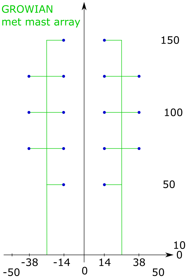
Figure 1 Sketch of the met mast array of the GROWIAN measurements. The blue dots indicate the positions of the wind speed measurement devices at four different horizontal and five different vertical positions.

The original question guiding our research was posed by the industry. Accordingly, the project focused on evaluating and improving the methods required by industrial certification guidelines (IEC), ensuring they are both reliable and computationally efficient enough to be used in design processes. Accordingly, further sources of turbulent wind data (e.g., constrained fields or large-eddy simulation (LES) wind fields) are not used within the scope of this paper. However, the use of different wind data will be the topic of discussion for follow-up work and articles (see, e.g., Bock et al., 2026). Depending on the source and characteristics of other turbulent wind fields, the aerodynamic coupling within the simulation may have to be adapted from prescribed BEM methods to actuator disk or actuator line methods.

3 Damage equivalent loads: differences between measured and simulated data

The main motivation of our research is to improve our understanding of the differences between the simulated (e.g., using Kaimal wind fields) and the measured loads at the full-scale Nordex turbine. In the following, we demonstrate such discrepancies between the simulated and the measured data. Specifically, we investigate bending moments at the main shaft of the wind turbine, i.e., the tilt and the yaw moments. For simplicity, we refer to the yaw and tilt moments at the main shaft as T_yaw and T_tilt. Moreover, we use the subscripts “m” and “s” to refer to measured loads and simulated loads, respectively. Two subscripts thus identify the moments. For example, the measured yaw moment is noted as T_m,yaw, while T_s,tilt indicates the simulated tilt moment.

The starting point of the comparison between measurements and simulations is based on the DEL defined in Sect. 2.1. Due to the significant potential effects on the turbine, particular interest is given to large-amplitude events within the load signals. To give predominance to such large-amplitude events within the calculation of the DELs, a Wöhler exponent m=10 is used for the analysis (see Eq. 1). Then, the DELs are referred to as DEL10.

Although the DEL with exponent m=10 is not a common choice for loads at the main bearing, we chose to use the DEL primarily as a tool to detect uncommonly large load events and did so for the following reasons: it is a standard tool available in each post-processing chain, and it yields a scalar number which can easily be evaluated for each load situation. This makes it much simpler to identify large load events than through time series analyses and study of load distributions.

Next, the DEL10 is conditioned by the simultaneous wind conditions. Each DEL10 calculated from a 10 min load signal is then classified into so-called wind bins. The wind bins are defined by the characteristics of the wind speed time series u(t), i.e., the mean ($\stackrel{\mathrm{‾}}{u}$) and the turbulence intensity (TI). The turbulence intensity is calculated as $\text{TI}={\mathit{\sigma }}_u/\stackrel{\mathrm{‾}}{u}$, where σ_u is the standard deviation. Both quantities, $\stackrel{\mathrm{‾}}{u}$ and TI, are calculated at hub height over the individual 10 min periods. Equally spaced wind bins with a size of $\mathrm{\Delta }\stackrel{\mathrm{‾}}{u}=\mathrm{1}\mathrm{m}{\mathrm{s}}^{-\mathrm{1}}$ and ΔTI=2 % are defined; e.g., $\stackrel{\mathrm{‾}}{u}=\mathrm{7.0}\pm \mathrm{0.5}\mathrm{m}{\mathrm{s}}^{-\mathrm{1}}$ and $\mathrm{TI}=\mathrm{9}\pm \mathrm{1}\mathit{\%}$.

Changes in wind conditions are expected to be reflected in the calculated DEL10. To prove this, we evaluate the DEL10 from simulated data for different combinations of $\stackrel{\mathrm{‾}}{u}$ and TI. We consider nine $\stackrel{\mathrm{‾}}{u}$–TI combinations within the wind bin of $\stackrel{\mathrm{‾}}{u}=\mathrm{8}\pm \mathrm{0.5}\mathrm{m}{\mathrm{s}}^{-\mathrm{1}}$ and $\text{TI}=\mathrm{10}\pm \mathrm{1}\mathit{\%}$. Eight realizations of IEC Kaimal turbulent fields with each $\stackrel{\mathrm{‾}}{u}$–TI combination are generated. The conditions of $\stackrel{\mathrm{‾}}{u}$ and TI are imposed at the height of 125 m. The effect on the loads of the turbine is simulated via the alaska/Wind BEM simulation. Figure 2 shows the resulting DEL10 of the simulated T_s,tilt for the different wind conditions. The horizontal green and red lines depict the global minimum, DEL10=0.087, and global maximum, DEL10=0.154, over the 72 realizations of the wind bin.

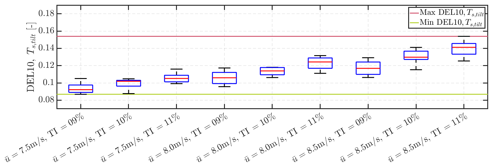
Figure 2 DEL10 of the simulated tilt moment (T_s,tilt) at the main shaft of the model wind turbine. Nine $\stackrel{\mathrm{‾}}{u}$–TI combinations are evaluated within the wind bin $\stackrel{\mathrm{‾}}{u}=\mathrm{8}\pm \mathrm{0.5}$ m s⁻¹ and TI $=\mathrm{10}\pm \mathrm{1}\mathit{\%}$. The global minimal and maximal values of DEL10 are marked by the green and the red horizontal lines, respectively. On each box, the red mark shows the median, and the bottom and top edges indicate the 25th and 75th percentiles. The whiskers indicate the most extreme data points.

The DEL10 from the measured moments are now compared to the results from the simulated moments. Figure 3a shows the probability density function (PDF) of the DEL10 of the measured T_m,tilt for the same wind bin of $u=\mathrm{8}\pm \mathrm{0.5}$ m s⁻¹ and $\text{TI}=\mathrm{10}\pm \mathrm{1}\mathit{\%}$ investigated before for the simulated T_s,tilt. The corresponding results for the measured and simulated yaw moment (T_m,yaw and T_s,yaw) are shown in (b). A set of 149 time series from the full-scale Nordex turbine belongs to this bin. As observed, the PDFs of the DEL10 from the measured T_m,tilt and T_m,yaw spread out further than the PDFs of the simulated T_s,tilt and T_s,yaw. While changing the choice and distribution of conditions within the wind bin may change the maximal value of the PDF of the simulated data and bring it closer to the measured one, the right tail of the distribution of the measurements stays unreachable (i.e., DEL10 values exceeding 0.16 do not appear in simulations using synthetic wind fields, for either the tilt or the yaw moment).

As mentioned previously, the selection of the exponent m=10 was intended to focus on the large-amplitude events of the load signal for the calculation of the DELs (see Eq. 1). It is acknowledged that atypical large-amplitude loads may induce undesirable effects on the turbine, and there is a clear necessity for manufacturers and operators of wind turbines to enhance their understanding of such effects. At this point, we have demonstrated significant differences between the simulated and measured loads under comparable standard wind conditions. The discrepancies are observed when comparing the DEL10 values. By definition, large-amplitude events within the signal dominate the calculated DEL10 when a high value of the Wöhler exponent, e.g., m=10, is used as explained in Sect. 2.1. The next step is to identify and investigate the characteristics of the large-amplitude load events, which, as shown in Fig. 3, are measured in operating full-scale circumstances but underestimated by the numerical simulations.

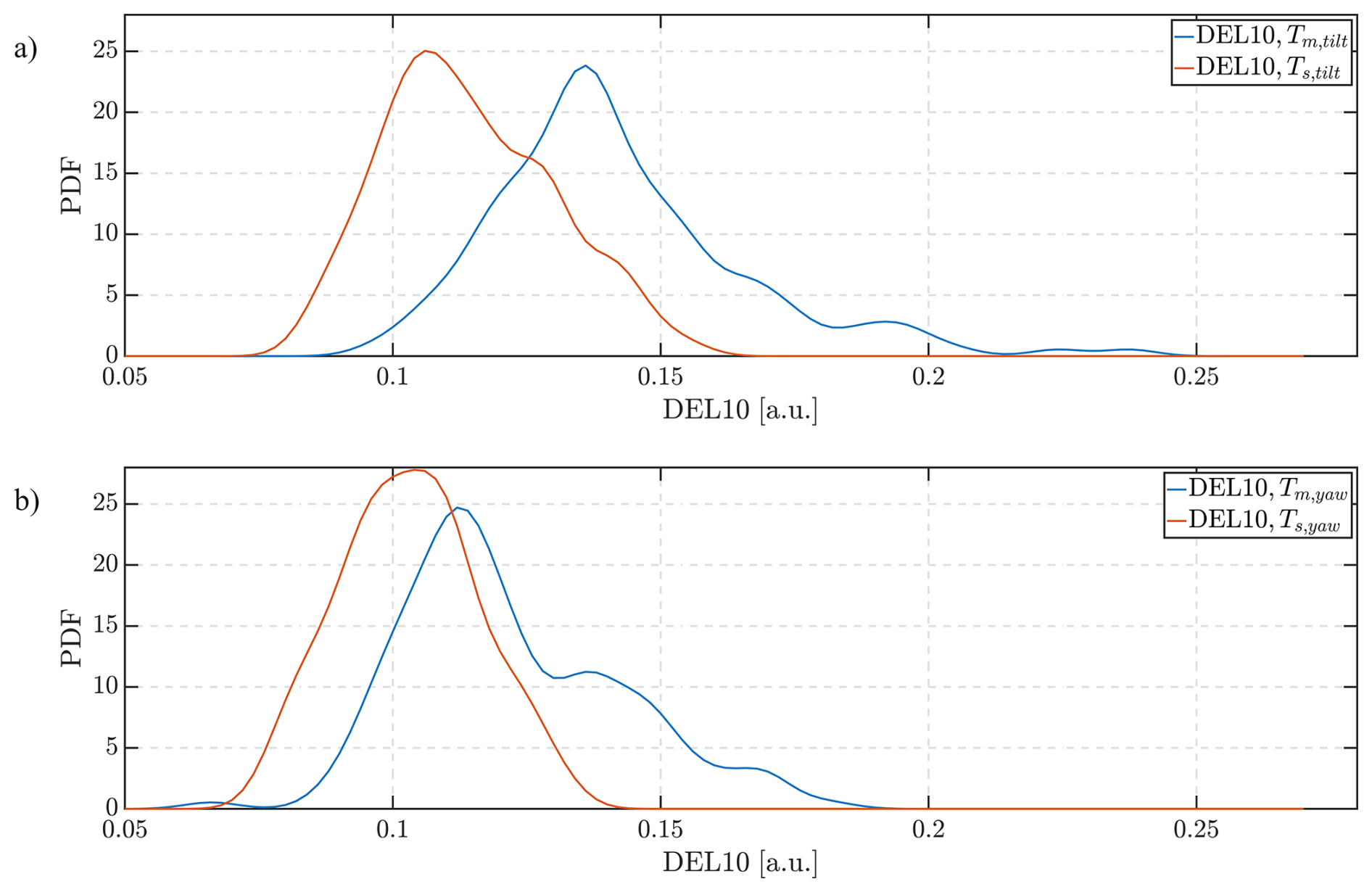
Figure 3 Probability density function (PDF) of the normalized DEL10 for the measured moments T_m,tilt and T_m,yaw of the full-scale operating Nordex wind turbine (blue line) and PDF of the normalized DEL10 of the simulated moments T_s,tilt and T_s,yaw (red line) for the wind bin $u=\mathrm{8}\pm \mathrm{0.5}$ m s⁻¹ and TI $=\mathrm{10}\pm$ 1 %. Subplot (a) contains the tilt moment and (b) the yaw moment.

4 What is dominating the damage equivalent loads?

Having identified the differences in the DEL10 between simulated and measured loads, we now investigate the origin of the large DEL10 values within the measured data. To do so, we analyze the time series of the measured T_m,tilt and T_m,yaw whose DEL10 values exceed the maximal DEL10 values of the corresponding simulated T_s,tilt and T_s,yaw.

Interestingly, we found load events that appear as isolated “bumps” within those selected time series of T_m,tilt and T_m,yaw. An example of such a bump is presented in Fig. 4. The bump structure lies inside the shadowed interval. The typical timescale of those bump events ranges from 20 to 50 s and tends to shorten with higher wind speeds. Automated detection of the bump structures can be implemented by fixing an amplitude threshold to the peaks of a filtered version of the signal.

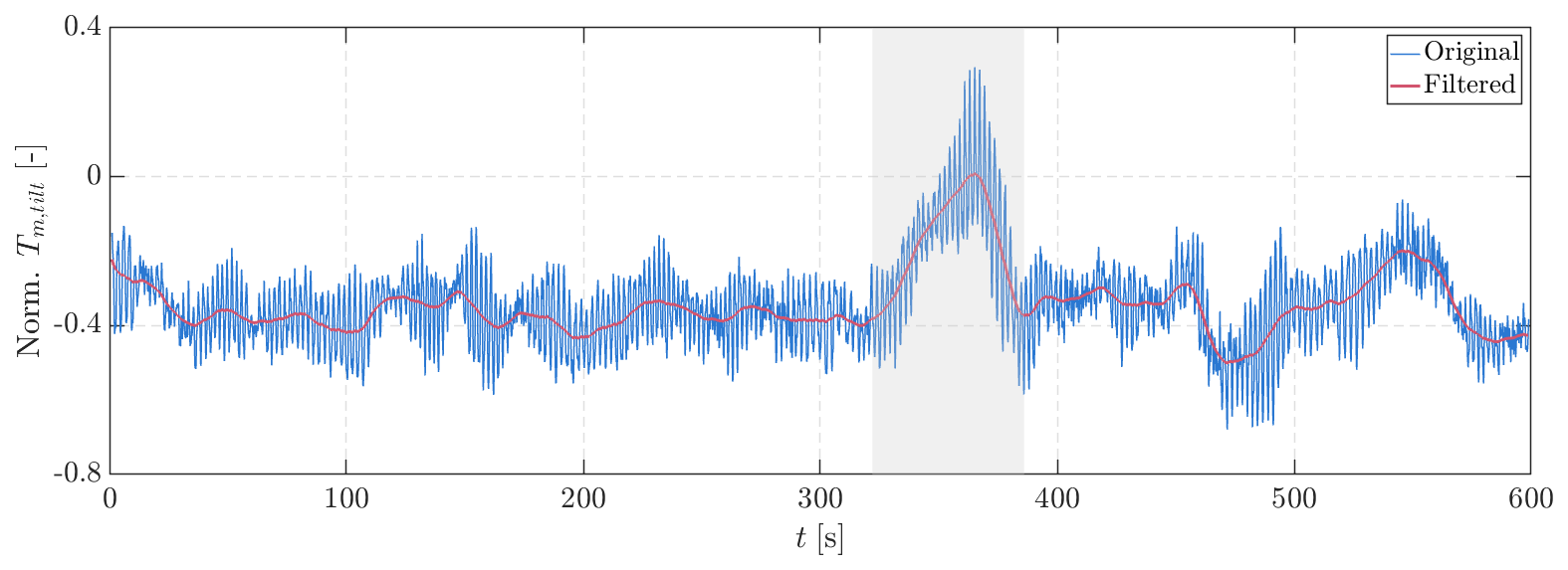
Figure 4 Normalized 10 min time series of the measured tilt moment (T_m,tilt) at the full-scale Nordex turbine with a DEL10 =0.22 and an observable bump event enclosed by the shadowed area. The time series belongs to the wind bin $\stackrel{\mathrm{‾}}{u}=\mathrm{8}$m s⁻¹ and TI =10 %. The blue line shows the original 20 Hz signal. The red line depicts a low-pass-filtered version of the signal with a cutoff frequency of 0.1 Hz.

Then, the following questions arise. What is the contribution of such bumps to the DEL10? Are such bumps the main drivers of the calculated DEL10? According to Eq. (1), the calculation of the DEL10 is defined as the aggregate of the amplitudes s_i within the signal weighted to the power of m; i.e., DEL10$\propto \sum n_i{s}_i^{m=\mathrm{10}}$. Therefore, the largest amplitude s_i within the time series dominates the DEL10. As will be proved, the global maximal and minimal values within the load signal delineate the largest amplitude driving the DEL10.

To demonstrate this, we take the exemplary 10 min time series of the measured T_m,tilt, shown in Fig. 4. Artificial load signals with a similar high-frequency component and successively added bumps with the same global maximum and minimum are generated and compared. The artificial signals are generated using two components:

• i.

  a high-frequency contribution characterized by a 3P frequency (i.e., 3 times the rotational frequency of the main shaft), with an amplitude which equals the mean amplitude of the 3P frequency within the measured T_m,tilt (calculated, e.g., by FFT)

• ii.

  a low-frequency contribution with the mean equal to the mean of the measured T_m,tilt and additional smooth bumps generated using fifth-order polynomials.

The comparison of T_m,tilt to the three artificial signals is shown in Fig. 5. In (a), only the high-frequency component and the mean value are used. In (b), the artificial signal contains only the largest low-frequency positive bump, i.e., over the mean. In (c), the artificial signal contains both the largest positive and the largest negative low-frequency bumps, i.e., below the mean. In (c), the global minimum and maximum of T_m,tilt and the artificial signals are equivalent, with values of −0.68 and 0.29, respectively. The calculated DEL10 values are given in the legends of the plots. As shown in Fig. 5, if the minimum and maximum of the measured and artificial signals do coincide, their DEL10 will almost be the same. In the example in (c), the values of the DEL10 differ by 3 % between T_m,tilt and the artificial signals, whereas the signal without any bump in (a) only reaches approximately 40 % of the DEL10 of T_m,tilt.

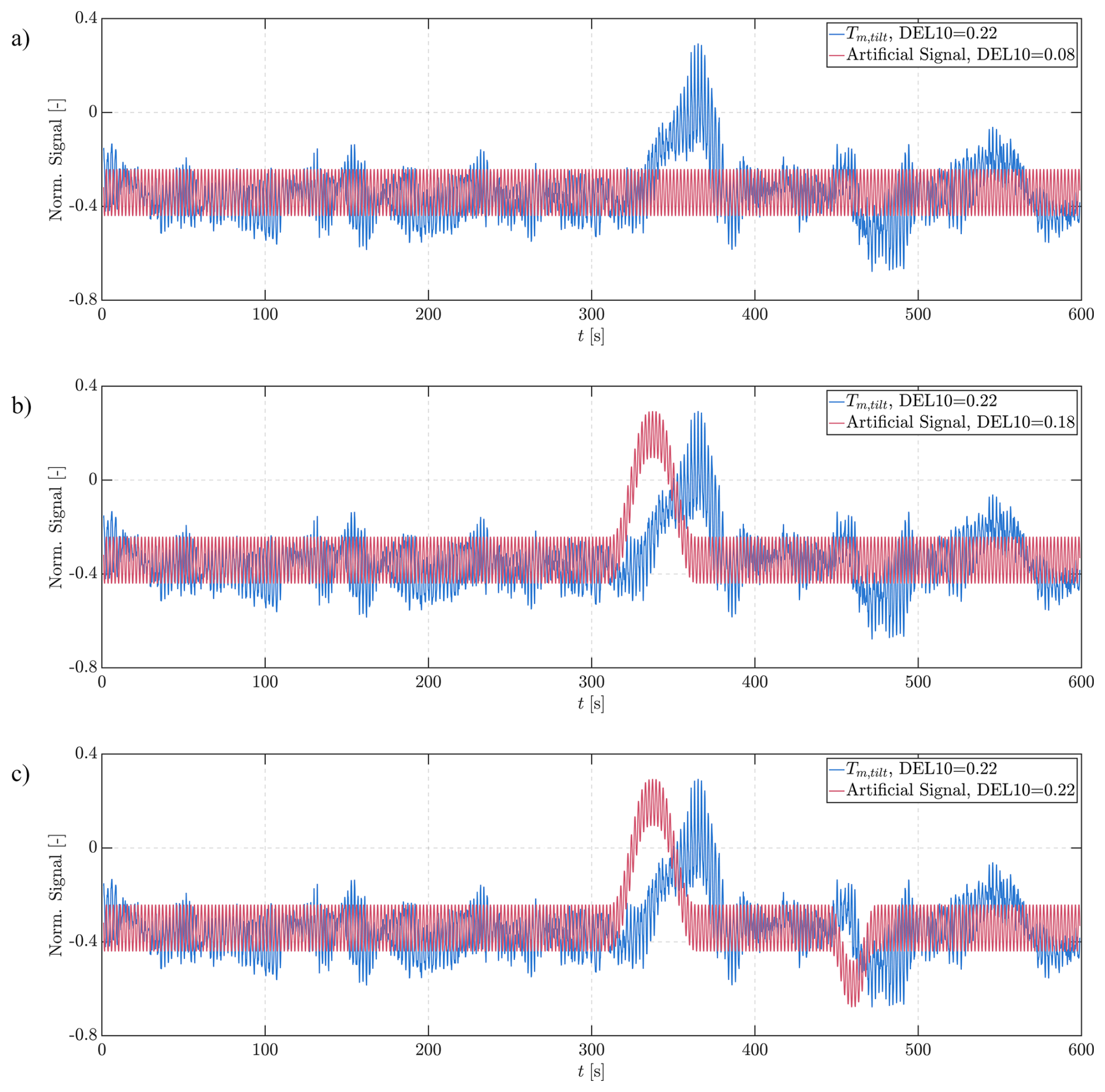
Figure 5 Comparison of the normalized measured signal T_m,tilt at the full-scale Nordex turbine (blue line) and three artificial signals (red lines). (a) The artificial signal only contains the high-frequency component and the mean value shift. (b) The artificial signal with the added largest positive low-frequency bump between 300 and 400 s. (c) The largest negative low-frequency bump is also added to the artificial signal at around 450 s. The resulting DEL10 values are given in the legends of the plots. “Positive” and “negative” bumps refer to structures over and below the mean value.

In addition, we show the extent to which other metrics are suitable or unsuitable for detecting the load extremes identified here. To do this, we use three different metrics:

• the global maximum minus global minimum of the load signal (max–min)

• damage equivalent load with exponent 4 (DEL4) as a common value for the main shaft of wind turbines

• damage equivalent load with exponent 10 (DEL10).

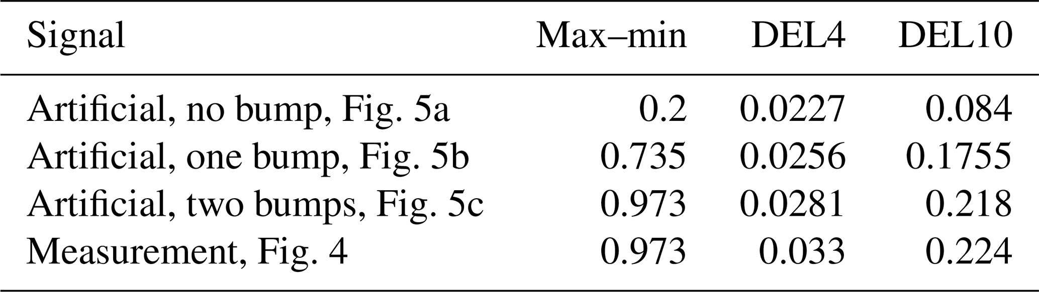
We used all three metrics on the four different signals of Fig. 5, i.e., the artificial signals with no bump, with one bump, with two bumps, and the measurement. The results are shown in Table 1. As can be seen, the DEL4 values increase by adding bumps to the artificial signal but not sufficiently to meet the measured value. The DEL4 depends much more on the fluctuations of amplitudes of the high-frequency component. Therefore, the DEL4 metric is not well suited for identifying extreme low-frequency dynamics. The metrics max–min and DEL10 are both well suited for detecting the type of extreme loads shown. There is a clear distinction between the different artificial signals. The artificial signal with two bumps has comparable values to the measurement in both metrics, max–min and DEL10.

Table 1 Comparison of load metrics: max–min, DEL4, and DEL10 used on the three different artificial signals (see Fig. 5) and the measurement signal of tilt moments.

Further analysis of multiple signals of the measured T_m,tilt and T_m,yaw suggested that the global maximum and minimum, which drive the DEL10, are delineated by two characteristics of the load signal: the amplitudes of the high-frequency content and the dynamics of the low-frequency component. The high-frequency contribution of the tilt and yaw moment at the main shaft is mainly induced by the rotation of the three blades as they pass through turbulent eddies (Burton et al., 2011). The low-frequency part, however, is driven directly by changes in the incident flow in the rotor plane.

To isolate the low-frequency contribution, we apply a Butterworth low-pass filter (Butterworth, 1930) to the load signals. The cutoff frequency is 0.1 Hz. This value is lower than the 1P frequency, i.e., rotational frequency, of the turbine. The filter is applied forward and backward to the signals so as not to run into time shifts. A filtered version of a load signal is shown in Fig. 4 for a 10 min time series of the measured T_m,tilt. In Sect. 5.2, we resume the discussion about the filtered signals of the bending moments and their correlation to structures in the incoming wind.

5 The virtual center of wind pressure

In the previous section, we highlighted the fact that bump events in the corresponding load time series dominate the damage equivalent loads. In the present section, we aim to relate such bump events to specific characteristics of the wind field itself. Further investigation of the measured data from the Nordex turbine (i.e., of additional load sensors) showed that significant changes in the bending moments at the main shaft coincide with specific events on the bending moments of the individual blades. These events in the loads on the blades were found to be correlated with specific azimuthal sections within a revolution. This observation led to the formulation of a hypothesis that wind structures appearing exclusively in specific regions of the rotor plane might explain the occurrence of the load bumps in the bending moments, i.e., T_m,tilt and T_m,yaw, at the main shaft.

The discussion concerning the origin of these unusual bump events on the measured loads has prompted the need to obtain information not only on the wind speed at different heights, as is the case for the met mast data provided at the site of the Nordex turbine (see Sect. 2.3), but also on how the wind speed is distributed in the rotor plane. To this end, a study was conducted on GROWIAN wind measurements based on a double-met-mast array. This configuration allows for the investigation of spatial wind structures, not only in the conventional vertical direction but also in their horizontal dimension. More details on the GROWIAN data are provided in Sect. 2.3.

The investigation of wind fields from the GROWIAN met mast array further supported the hypothesis that the persistent bend of the whole rotor and, thus, the main shaft must be related to a large wind structure, i.e., a change in the wind speed in significant areas of the rotor plane. Further correlations between the main shaft bending moments and spatial wind structures are discussed in Sect. 5.2.

5.1 Definition

To quantify the impact of the assumed large-scale wind structures driving the bending of the main shaft, we use the well-known concept of center of pressure from fluid mechanics (Anderson, 1991).

The center of pressure of a body is the point at which a single force acting at that point can cause the same effect as the original pressure field. Analogously, the total force acting on a body at the center of pressure is the surface integral of the pressure field across the body's surface. In a similar way, the effect of a wind field over the rotor disk of a turbine is reduced to a point-wise force acting at the virtual center of wind pressure (CoWP). As we outline below, our definition of the CoWP will lead to a non-physical distance from the hub. For this reason, we refer to it as a virtual center. The concept is illustrated schematically in Fig. 6.

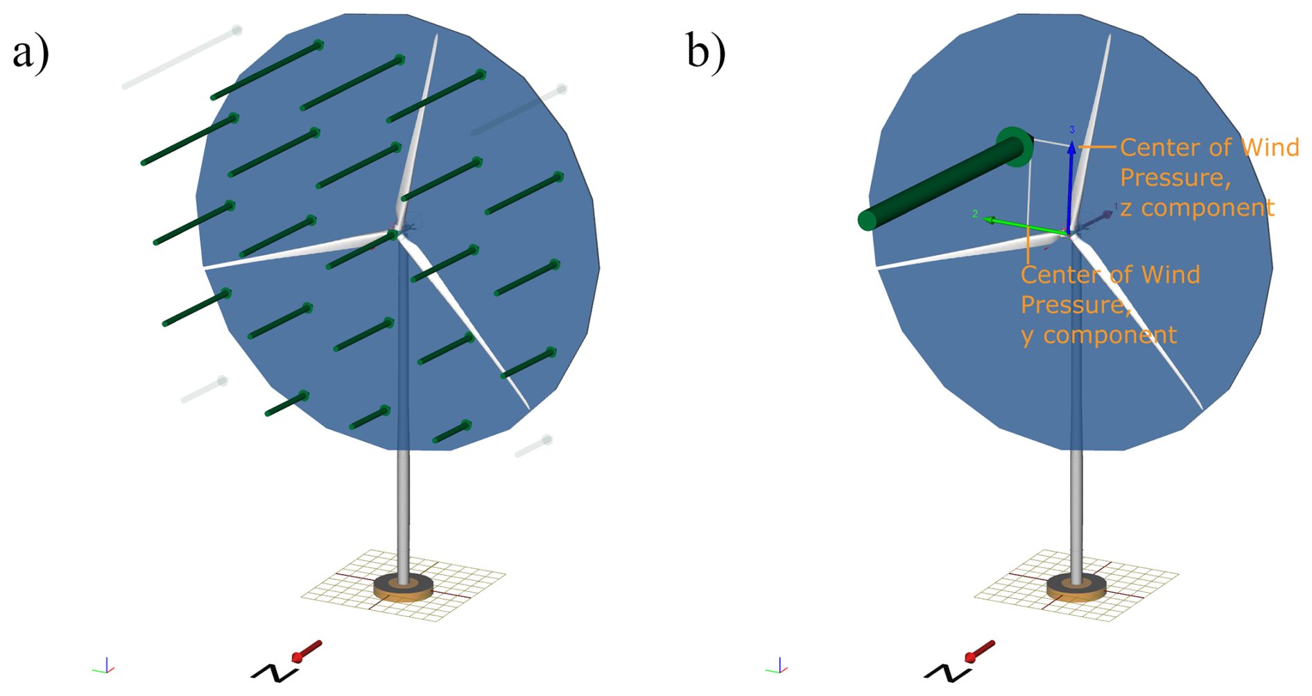
Figure 6 Schematic representation of the CoWP from a wind field acting on the rotor disk. (a) Illustration of the discrete thrust forces acting on defined grid points (y–z). (b) The collective effect of the individual thrust forces in (a) is replaced by a single aggregated thrust force acting on the CoWP.

In the following, we explain how to estimate the CoWP. As shown in Fig. 6, we define the surface A of the rotor disk, i.e., given by the hub height and rotor radius as the surface of the body within the wind flow. This clarifies that, in the context of this paper, we assume the concept of dynamic pressure on an actuator disk (Sorensen, 2012). We can now calculate the yaw and tilt moments at the center of the disk (o), which are induced by the dynamic pressure on the surface. They are referred to as the virtual-pressure-induced moments. At this point, we introduce the subscript “v” for virtual. Then, the two virtual moments T_v,tilt and T_v,yaw are defined as

$$\begin{array}{}\text{(2)}& {\displaystyle }{T}_{\mathrm{v},\mathrm{tilt}}\left(t\right)=\underset{A}{\int }z\cdot {\displaystyle \frac{\mathit{\varrho }}{\mathrm{2}}}\cdot u^{\mathrm{2}}(y,z,t)\mathrm{d}A,\text{(3)}& {\displaystyle }{T}_{\mathrm{v},\mathrm{yaw}}\left(t\right)=-\underset{A}{\int }y\cdot {\displaystyle \frac{\mathit{\varrho }}{\mathrm{2}}}\cdot u^{\mathrm{2}}(y,z,t)\mathrm{d}A,\end{array}$$

where z and y are, respectively, the vertical and horizontal positions within the rotor disk with origin o; ϱ is the air density; and $u(y,z,t)$ is the normal component to A of the wind field defined at the y–z plane.

Now, the continuous definitions of the virtual-pressure-induced moments are translated into their discrete versions as

$$\begin{array}{}\text{(4)}& {\displaystyle }{T}_{\mathrm{v},\mathrm{tilt}}\left(t\right)=\sum _{i=\mathrm{1}}^n{z}_i\cdot {\displaystyle \frac{\mathit{\varrho }}{\mathrm{2}}}\cdot u^{\mathrm{2}}(y_i,z_i,t)\cdot \mathrm{\Delta }{A}_i,\text{(5)}& {\displaystyle }{T}_{\mathrm{v},\mathrm{yaw}}\left(t\right)=-\sum _{i=\mathrm{1}}^n{y}_i\cdot {\displaystyle \frac{\mathit{\varrho }}{\mathrm{2}}}\cdot u^{\mathrm{2}}(y_i,z_i,t)\cdot \mathrm{\Delta }{A}_i,\end{array}$$

where n is the number of discretized grid points defined at (y_i,z_i), which lie inside the rotor area A. ΔA_i is the discretized section of the rotor area A.

Generally, a moment T can be rewritten as the outer product of a point force F and a lever r as $\mathit{T}=\mathit{r}\times \mathit{F}$. For the virtual-pressure-induced moments, the force F is assumed as the thrust force F_thrust, normal to the rotor plane. F_thrust over the disk A is calculated as

$$\begin{array}{}\text{(6)}& F_{\text{thrust}}\left(t\right)=\sum _{i=\mathrm{1}}^n{\displaystyle \frac{\mathit{\varrho }}{\mathrm{2}}}\cdot u^{\mathrm{2}}(y_i,z_i,t)\cdot \mathrm{\Delta }{A}_i.\end{array}$$

Then, the y and z components of the lever r can be calculated from T_v,tilt and T_v,yaw, respectively, and F_thrust. This two-dimensional position at which F_thrust acts inside the rotor area A corresponds to the CoWP. The two components of the CoWP, i.e., CoWP_z and CoWP_y, are calculated as

$$\begin{array}{}\text{(7)}& \begin{array}{rl}{\mathrm{CoWP}}_z\left(t\right)& ={\displaystyle \frac{\sum _{i=\mathrm{1}}^n{z}_i\cdot \frac{\mathit{\varrho }}{\mathrm{2}}\cdot u^{\mathrm{2}}(y_i,z_i,t)\cdot \mathrm{\Delta }{A}_i}{\sum _{i=\mathrm{1}}^n\frac{\mathit{\varrho }}{\mathrm{2}}\cdot u^{\mathrm{2}}(y_i,z_i,t)\cdot \mathrm{\Delta }{A}_i}}\\ {\mathrm{CoWP}}_y\left(t\right)& =-{\displaystyle \frac{\sum _{i=\mathrm{1}}^n{y}_i\cdot \frac{\mathit{\varrho }}{\mathrm{2}}\cdot u^{\mathrm{2}}(y_i,z_i,t)\cdot \mathrm{\Delta }{A}_i}{\sum _{i=\mathrm{1}}^n\frac{\mathit{\varrho }}{\mathrm{2}}\cdot u^{\mathrm{2}}(y_i,z_i,t)\cdot \mathrm{\Delta }{A}_i}}\end{array}\end{array}$$

and

$$\begin{array}{}\text{(8)}& \begin{array}{rl}{T}_{\mathrm{v},\mathrm{tilt}}\left(t\right)& ={\mathrm{CoWP}}_z\left(t\right)\cdot F_{\text{thrust}}\left(t\right)\\ T_{\mathrm{v},\mathrm{yaw}}\left(t\right)& =-{\mathrm{CoWP}}_y\left(t\right)\cdot F_{\text{thrust}}\left(t\right).\end{array}\end{array}$$

The CoWP and the virtual moments (T_v,tilt and T_v,yaw) can be calculated purely from measured or synthetic wind fields $u(y_i,z_i,t)$. In that way, the introduced concepts serve as tools for characterizing and comparing wind structures within different wind fields (e.g., under different atmospheric or orographic conditions or synthetic fields generated with different wind models). Furthermore, the surface area A for calculating the CoWP can be adapted to different setups within experiments or measurement configurations. For example, the FINO measurements are recorded at different heights by several anemometers that are vertically aligned (FINO, 2025). Therefore, in this case, the domain A can be changed to a vertical line to characterize the one-dimensional dynamics of the CoWP within the atmospheric inflow.

For the analysis of other load sensors or further applications, it may be meaningful to derive a more complex variation of the CoWP. Therefore, it may be necessary to vary the domain A or introduce a drag or thrust coefficient C_T to the pressure term (the term $\frac{\mathit{\varrho }}{\mathrm{2}}\cdot u^{\mathrm{2}}$ is replaced by $\frac{\mathit{\varrho }}{\mathrm{2}}\cdot C_{\mathrm{T}}\cdot u^{\mathrm{2}}$ in each formula). Thus, the wake effect of the turbine rotor could be considered by using the thrust coefficient of the wind turbine rotor or the axial induction of the BEM of the full rotor. Another extension to a turbine-dependent concept could be to change the domain to the rotor blades or discretized blade stations and use the thrust force at each blade station.

An example of the estimation of the out-of-plane bending moment of the rotor via the triaxial asymmetry index was introduced in Lavely (2017). The out-of-plane bending moment is defined as $\sqrt{T_{\text{tilt}}^{\mathrm{2}}+T_{\text{yaw}}^{\mathrm{2}}}$.

5.2 Correlation between the center of wind pressure and the bending moments

In this section, we investigate the correlation between the introduced CoWP, as a feature of the wind, and the induced bending moments at the main shaft of the wind turbine. To calculate the CoWP, spatially distributed information of the wind speed is necessary. Thus, field measurements of the full-scale wind turbine, including turbine loads T_m,tilt and T_m,yaw, cannot be used here, as the met mast only captured wind speeds at three points along a vertical line.

Therefore, the correlation between the CoWP and the bending moments is demonstrated using the GROWIAN wind measurements (see Sect. 2.3). To this end, the 334 blocks of 10 min wind measurements from the double-met-mast array were reconstructed as wind fields and applied within the alaska/Wind BEM simulator. As can be seen from the setup of the GROWIAN met mast array in Fig. 1, the measurement campaign covered an area with the dimensions of 76 m in the horizontal and 100 m in the vertical direction. To be used as turbulent wind within the load simulation, the positions of the grid points were modified. We multiplied the horizontal distance of grid points by a factor of 2 and the vertical distance by a factor of 1.5. By using the modified coordinates, the stretched GROWIAN grid has a horizontal dimension of 152 m and vertical dimension of 150 m, which is sufficient to cover the rotor with 149 m diameter. To retrieve wind speeds at arbitrary positions within the rotor disk, a linear interpolation between the four neighboring grid points is used. This is the standard procedure to retrieve wind speeds at blade stations within the simulation for all synthetic and reconstructed turbulent wind fields. After applying the GROWIAN turbulent fields in the simulation, the DEL10 values from the signals of the tilt and yaw moments at the main shaft were calculated.

Interestingly, within the GROWIAN-simulated loads, we observed bump events on the signals, together with DEL10 values that exceed the DEL10 from IEC Kaimal-simulated loads when using comparable environmental conditions (i.e., $\stackrel{\mathrm{‾}}{u}$ and TI). These findings agree with the results shown in Sect. 3, where large values of the DEL10 from the measured T_m,tilt and T_m,yaw at the full-scale operating turbine are not observed within the simulated T_s,tilt and T_s,yaw with IEC Kaimal wind fields. Further comparisons of a GROWIAN time series, showing large DEL10 values, to turbulent Kaimal wind fields generated using the same environmental conditions are shown in Sect. 5.3. In Fig. 12, it can clearly be seen that the Kaimal wind fields cannot be distinguished from the GROWIAN field using the time series of wind speed at hub height or average mean wind speed. In contrast, the time series of the CoWP of the GROWIAN wind field shows a bump-like behavior which is not reproduced in amplitude by any of the Kaimal fields.

As we have access to the full GROWIAN wind field, we are able to compare the virtual moments (T_v,tilt and T_v,yaw), the CoWP, and the simulated moments (T_s,tilt and T_s,yaw). We repeat that for the rest of this section:

• the CoWP is calculated from the GROWIAN measurement data using Eq. (7)

• the virtual moments T_v,tilt and T_v,yaw are calculated from the GROWIAN measurement data using Eqs. (4) and (5)

• the simulated bending moments T_s,tilt and T_s,yaw at the main bearing are calculated through BEM simulations, where GROWIAN-reconstructed fields were applied as turbulent wind inflow.

In order to compare the three physically different signals, i.e., virtual moments, the CoWP, and simulated moments, we normalize the data. The normalization allows for a direct comparison of the dynamical behavior and a meaningful cross-correlation. The normalization of the individual 10 min signals is performed as follows:

1. low-pass filtering of the data with a cutoff frequency of 0.1 Hz (by doing so, the 3P content of the signals is removed)

2. subtraction of the mean value calculated over the 10 min length

3. normalization by the standard deviation calculated over the 10 min length.

Figures 7 and  8 show two exemplary 10 min periods of the three signals from the GROWIAN data. The wind conditions differ between the two examples. In Fig. 7, $\stackrel{\mathrm{‾}}{u}=\mathrm{12.9}$ m s⁻¹ and TI=6 %. And, in Fig. 8, $\stackrel{\mathrm{‾}}{u}=\mathrm{11.1}\mathrm{m}{\mathrm{s}}^{-\mathrm{1}}$ and TI=6 %. As observed in the two examples, the simulated moments T_s,tilt and T_s,yaw correlate to the respective virtual moments T_v,tilt and T_v,yaw. Remarkably, the simulated moments are derived after the interaction of the wind and the turbine, while the virtual moments are calculated entirely from the wind field. Furthermore, according to Eq. (8), a correlation between the CoWP and the virtual moments T_v,tilt and T_v,yaw was expected. However, the strong similarity seen in Fig. 7 and Fig. 8 reveals the dominance of the CoWP term over the thrust force F_thrust on the estimated virtual moments T_v,tilt and T_v,yaw. In other words, the low-frequency dynamics of the induced bending moment are driven by the CoWP's location rather than by the magnitude of the aggregated thrust force.

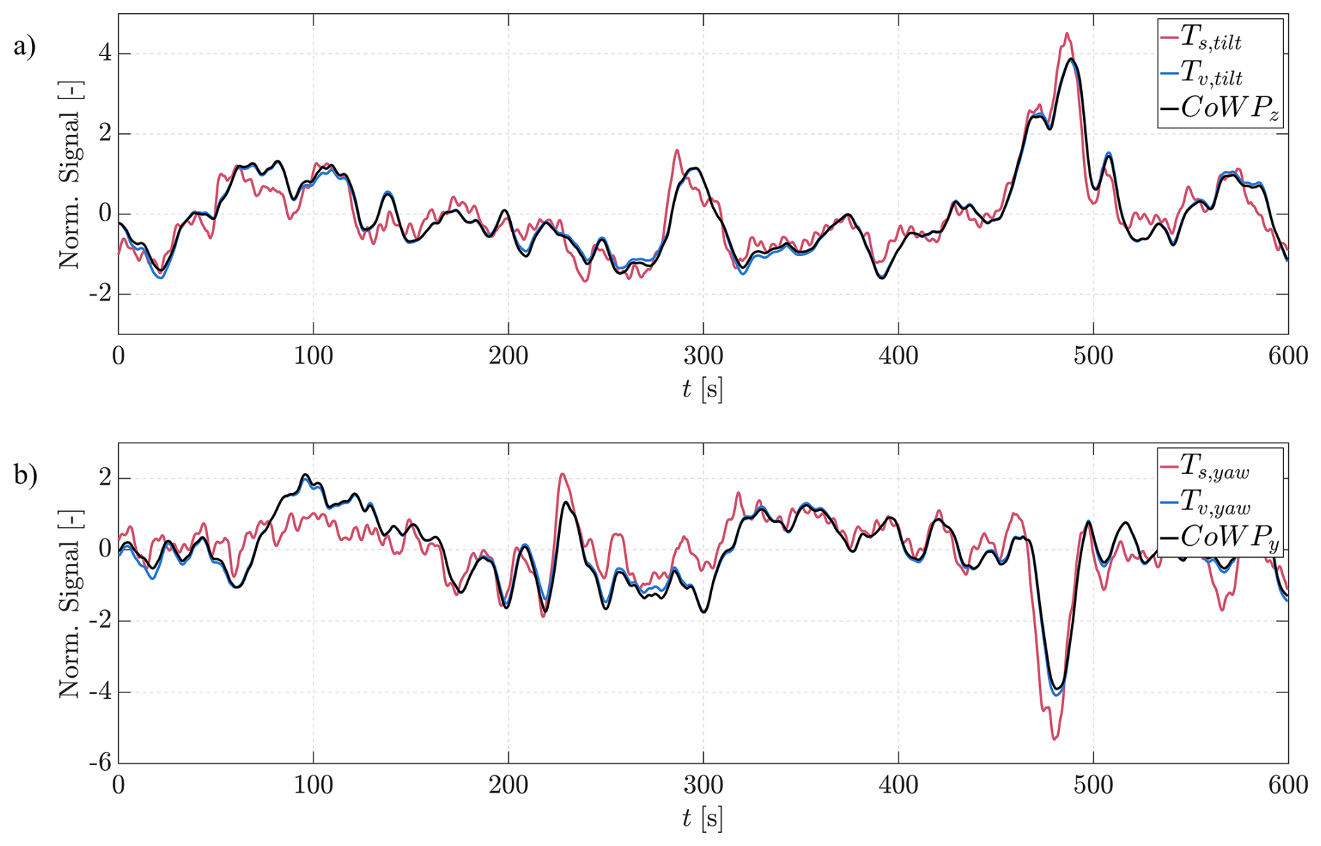
Figure 7 Comparison of the normalized signals: the simulated moments (T_s,tilt and T_s,yaw), the virtual-pressure-induced moments (T_v,tilt and T_v,yaw), and the center of wind pressure (CoWP). Data from a GROWIAN 10 min data set with $\stackrel{\mathrm{‾}}{u}=\mathrm{12.9}\mathrm{m}{\mathrm{s}}^{-\mathrm{1}}$ and TI=6 % at 125 m height. (a) The tilt moment and (b) yaw moment are compared.

Figure 8 Comparison of the normalized signals: the simulated moments (T_s,tilt and T_s,yaw), the virtual-pressure-induced moments (T_v,tilt and T_v,yaw), and the center of wind pressure (CoWP). Data from a GROWIAN 10 min data set with $\stackrel{\mathrm{‾}}{u}=\mathrm{11.1}\mathrm{m}{\mathrm{s}}^{-\mathrm{1}}$, and TI=6 % at 125 m height. (a) The tilt moment and (b) yaw moment are compared.

A measure of the correlation between the simulated moments (T_s,tilt and T_s,yaw) and the CoWP becomes relevant. We quantify the correlation between T_s,tilt and CoWP_z by calculating the cross-correlation function ρ(τ) between the two quantities as

$$\mathit{\rho }\left(\mathit{\tau }\right)={\displaystyle \frac{\mathrm{1}}{\stackrel{\mathrm{̃}}{n}}}\sum _{i=\mathrm{0}}^{\stackrel{\mathrm{̃}}{n}}\left({\mathrm{CoWP}}_z\right(i)\cdot T_{\mathrm{s},\mathrm{tilt}}(i+\mathit{\tau }\left)\right),$$

where $\stackrel{\mathrm{̃}}{n}$ is the number of time steps i within the signal, and τ is the number of lagging steps. The values of ρ(τ) range between 0 and 1. Afterward, the maximal value ρ_max of the cross-correlation function for each 10 min data set is calculated. Values of $\mathit{\tau }=[-\mathrm{20},\mathrm{20}]$s are considered. Then, we define

$${\mathit{\rho }}_{\max }=\underset{\mathit{\tau }\in [-\mathrm{20},\mathrm{20}]}{max}\left[\mathit{\rho }\left(\mathit{\tau }\right)\right].$$

Figure 9a shows the wind conditions $\stackrel{\mathrm{‾}}{u}$ and TI of each individual 10 min GROWIAN measurement at hub height (125 m) on the x and y axes. The color code shows the maximal correlation value ρ_max between the corresponding simulated T_s,tilt and the CoWP. For a better visualization of the distribution of ρ_max over the 334 GROWIAN data sets, the PDF of ρ_max is shown in Fig. 9b.

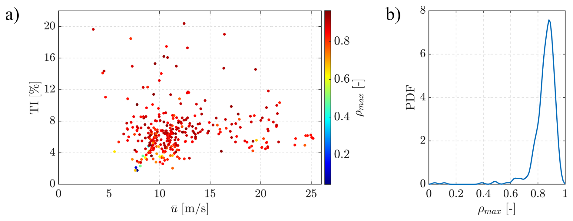
Figure 9 Maximum correlation coefficient ρ_max between the CoWP and the simulated tilt moment (T_s,tilt) for the 334 GROWIAN measurements. In (a), the position of the marker encodes the environmental conditions in terms of mean wind speed ($\stackrel{\mathrm{‾}}{u}$) and turbulence intensity (TI). The color represents the value of ρ_max. In (b), the PDF of ρ_max is shown.

For relevant conditions, we showed that the CoWP captures the dominant contribution to the load dynamics, which is underlined by the correlation coefficients in Fig. 9. Except for low turbulence intensities and wind speeds, the correlation coefficient appears relatively robust (ρ_max>0.6) concerning varying turbulence intensities and wind speeds. This includes even unstable atmospheric conditions corresponding to the cluster around 20 m s⁻¹ due to strong westerly wind gusts as reported by Koerber et al. (1988).

5.3 Comparison of synthetic wind fields to GROWIAN wind field

In this section, we address the following question: if there is an extreme load behavior, how can this be seen in the inflowing wind?

The challenge is that extreme or unusual behavior in loads or inflowing wind can only be determined statistically. To do so, each 10 min time series of measurements and simulations is binned using the statistical characteristics of mean wind speed at hub height and turbulence intensity. After that, the time series of different signals can be compared statistically. This will yield “normal” and extreme situations for the signals. Comparing this extreme situation to a considerable number of “normal” situations from the same wind bin will show if the extreme situations can also be identified using other characteristics – e.g., an extreme load can also be seen in characteristics of the inflowing wind. A one-to-one comparison of the extreme time series to one randomly selected “normal” time series cannot prove this statement.

Another challenge is that detailed information about the inflowing wind is not available for most field measurements. Met masts often provide only two or three vertically aligned measurements of at most hub height. This allows only for a few metrics of inflowing wind (such as wind speed at hub height) while disregarding those that require spatially measured inflowing wind, such as a rotor-averaged mean wind speed or the introduced CoWP.

To further demonstrate this, we selected a wind field measured within the GROWIAN campaign, which gives a comparably high tilt moment at the main bearing when used as inflowing wind in a load simulation. The conditions are 12.9 m s⁻¹ mean wind speed and 6 % turbulence intensity. The DEL10 of the simulated tilt moment has a value of 0.21, whereas the DEL10 of simulations using synthetic wind fields generated as described in Appendix A will not yield DEL10 values above 0.15. The tilt moment of the main bearing in Fig. 10 clearly shows an extreme load bump shortly before 500 s. The same GROWIAN data set and simulation results are used in Fig. 7.

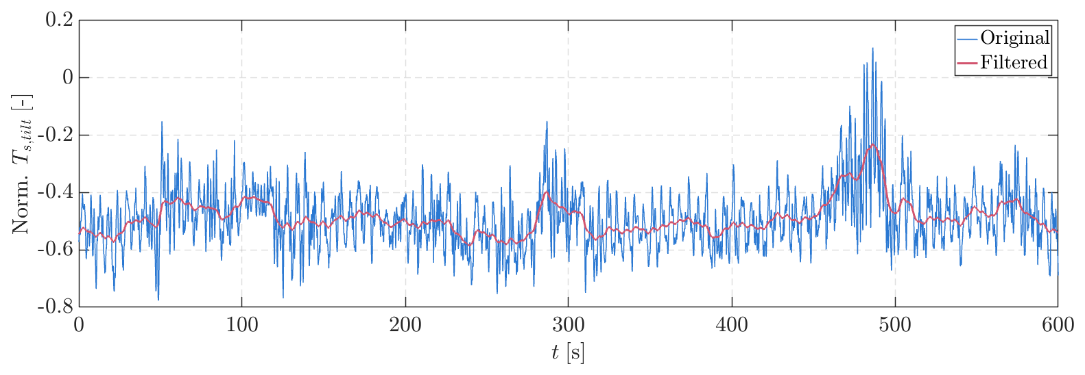
Figure 10 Normalized 10 min time series of the simulated tilt moment (T_s,tilt). Inflowing wind data from a GROWIAN 10 min data set with $\stackrel{\mathrm{‾}}{u}=\mathrm{12.9}\mathrm{m}{\mathrm{s}}^{-\mathrm{1}}$ and TI=6 % at 125 m height were used. The blue line shows the original 20 Hz signal. The red line depicts a low-pass-filtered version of the signal with a cutoff frequency of 0.1 Hz.

As shown in Sect. 5.2, the dynamic behavior of the low-frequency part of the load correlates well to the CoWP. Now we want to answer the question of whether the extreme event happening at approximately 500 s can be seen when analyzing the inflowing wind. To check this, we compare the GROWIAN measurement to 32 randomly generated synthetic wind fields, which all yield a “normal” load behavior. We performed the analysis with 32 Kaimal fields and 32 Mann fields, where details on the synthetic wind fields can be found in Appendix A.

To compare the inflowing wind in the most physical way possible, we adapt the calculation of characteristic properties to the GROWIAN measurements. This means that we change the domain A, which is used for calculation of the CoWP from the rotor disk, to a domain consisting of 16 squares with a size of 25 m × 25 m for the GROWIAN case and a similar domain A consisting of 10 m × 10 m squares for the synthetic wind fields – see Fig. 11 for more details.

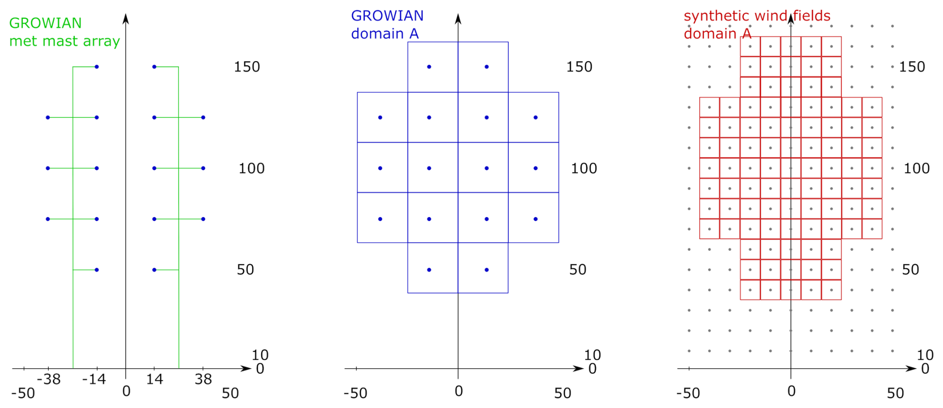
Figure 11 GROWIAN met mast array with 16 spatial wind speed measurements (left). Domain A for GROWIAN wind field consisting of 16 squares A_i of size 25 m × 25 m (middle). Domain A of synthetic Kaimal and Mann wind fields consisting of 10 m × 10 m squares with centers which lie inside domain A of GROWIAN (right).

We chose three different characteristics of the inflowing wind: the mean wind speed at hub height, the average wind speed, and the CoWP (using Eq. 7), where the last two were calculated in domain A. The three characteristics of the inflowing wind were calculated for all 32 synthetic fields and compared to the characteristics of the GROWIAN field. The results of the comparison are shown in Figs. 12 and 13.

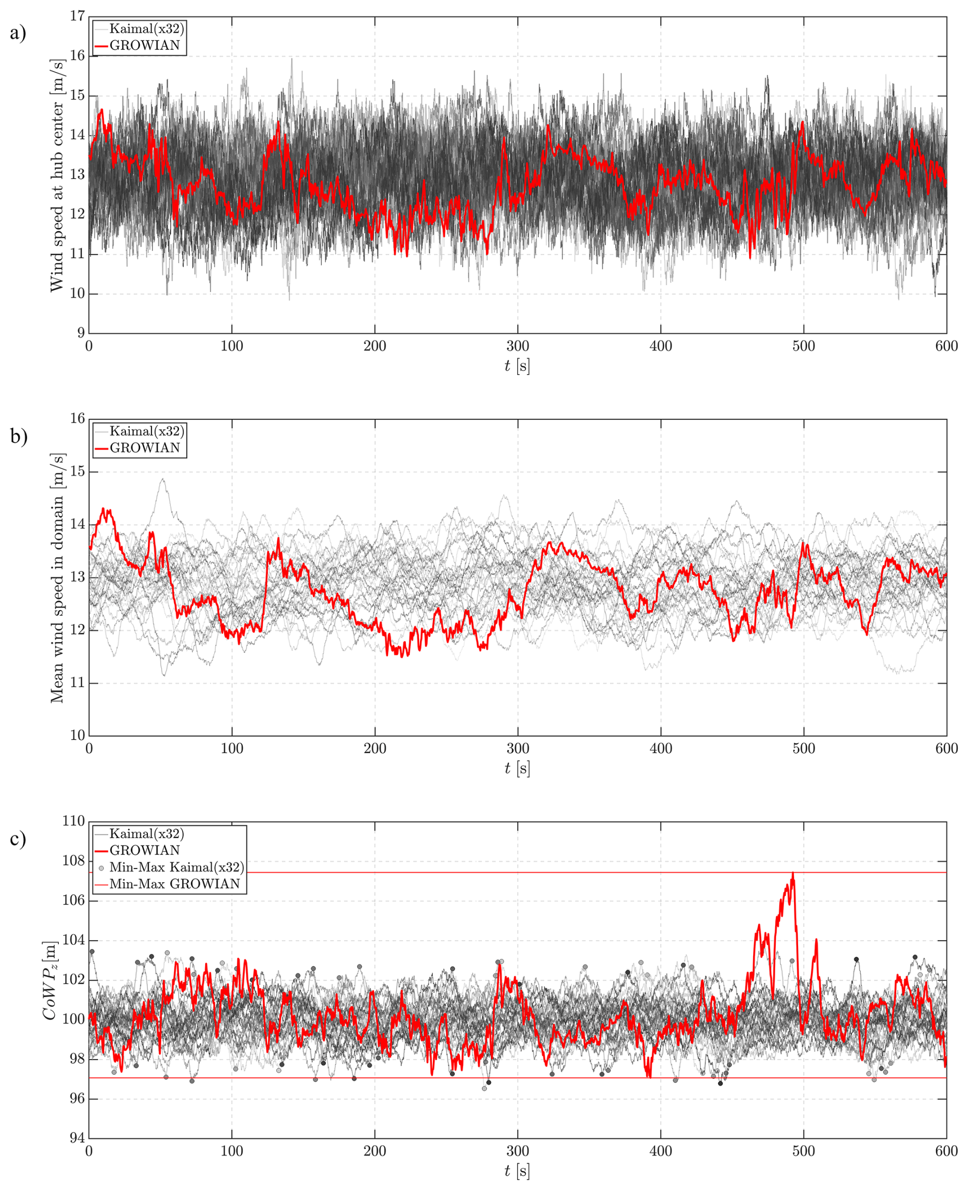
Figure 12 Comparison of 32 synthetic Kaimal wind fields (gray lines) to one GROWIAN measurement (red line) under conditions of 12.9 m s⁻¹ mean wind speed and 6 % turbulence intensity. (a) Wind speed at hub height, (b) mean wind speed over the domain of the GROWIAN measurement, and (c) CoWP_z for the domain of GROWIAN measurements.

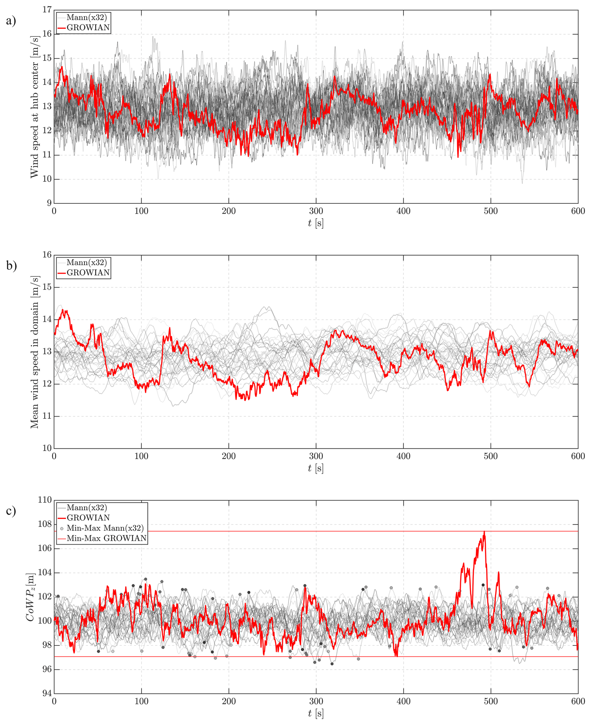
Figure 13 Comparison of 32 synthetic Mann wind fields (gray lines) to one GROWIAN measurement (red line) under conditions of 12.9 m s⁻¹ mean wind speed and 6 % turbulence intensity. (a) Wind speed at hub height, (b) mean wind speed over the domain of the GROWIAN measurement, and (c) CoWP_z for the domain of GROWIAN measurements.

As can be seen in Fig. 12a and b for the Kaimal fields and in Fig. 13a and b for the Mann fields, the wind at hub height and the mean wind speed in domain A of the red line representing the GROWIAN measurement do not show any extreme behavior. The extreme event at approx. 500 s cannot be detected in the time series. The red line does not leave the “block” generated by the 32 different versions of the synthetic fields. However, the red line of the CoWP in Figs. 12c and 13c shows an extreme behavior at approximately 500 s. This extreme event clearly exceeds the values of all Kaimal and Mann synthetic wind fields, respectively.

This example shows that there are turbulent wind conditions yielding extreme loads which cannot be detected by measuring mean wind speed and turbulence intensity at hub height. We point out that adding extreme operating events, such as extreme operating gusts defined by the standard IEC guidelines, will only change the mean wind speed for a certain time span – but will not change the CoWP as the changes in direction and wind speed occur uniformly over the rotor disk. As a result, they will change the aggregated thrust in the disk but not the position where the aggregated thrust on the rotor would act.

The effects on the turbine caused by the fluctuations of the estimated CoWP can be identified from the wind speeds of the grid points of the GROWIAN measurements. They show local effects – like jets – which are not yet covered by synthetic turbulent wind fields or extreme operating events.

The CoWP is a relatively simple feature that characterizes any wind field, defined over an arbitrary domain. This is particularly advantageous as measurement campaigns are conducted in different configurations, including vertically arranged measurements on a single met mast, equidistant grids as utilized in the GROWIAN campaign, and spatially distributed grids with various tiling, such as the new WiValdi meteorological mast array (WiValdi, 2023) or measurements enriched by lidar.

6 Conclusions and outlook

We have shown that for modern wind turbines, there are certain situations where applying state-of-the-art synthetic turbulent wind fields within BEM simulations fails to fully reproduce the spectrum of measured loads for given environmental conditions, characterized by mean wind speed and turbulence intensity. The industry standard procedure for such uncovered situations is to superpose extreme operating gusts and turbulent wind fields. In order to increase the accuracy and efficiency in the design process of wind turbines and to generate site-specific turbulent wind fields and load estimates, it is essential to understand the source of these differences.

We identified “bump” events by analyzing the time series of measured bending moments at the main shaft, whose DEL values are particularly large. We demonstrated through the comparison to artificial signals that these bump structures drive the large DEL. The bumps were not observed within simulated loads from standard wind fields, which reinforces the need for a more comprehensive understanding of the turbulent structures and the improvement of the synthetic wind fields.

Using spatiotemporally measured wind speeds from the GROWIAN campaign, we have correlated those load bump events to large structures within the wind field. To describe those structures, we introduced the virtual center of wind pressure and virtual-pressure-induced moments, which are obtained by a weighted average of the wind speed (more precisely, the thrust force) over the rotor disk. As the two quantities are independent of the turbine and are calculated from measurements or synthetic turbulent wind fields, they are an efficient tool to characterize large-scale structures within the wind fields.

The dynamic behavior of the virtual center of wind pressure strongly correlates with the main shaft moments of the wind turbine. In light of these results, we conclude that the current characterization of the inflow by single-point parameters, e.g., mean wind speed and turbulence intensity, does not account for events across the rotor plane and large-scale spatial structures within the wind that induce significant loads at the wind turbine. To close this gap, it would be desirable to extend the analysis of the center of wind pressure to synthetic wind fields that account for the empirically observed occurrence of extreme wind field fluctuations, which are currently underestimated in the statistical framework provided by Kaimal or Mann models of the IEC standard. One attempt to better cover realistic wind field fluctuations was recently presented in Friedrich et al. (2022).

Ongoing studies of the virtual center of wind pressure using atmospheric measurement campaigns will help to parameterize its statistical and dynamic characteristics within the atmospheric flow; see, e.g., Moreno et al. (2025). Synthetic turbulent wind fields, including realistic wind features, will be essential for further applications, such as more accurate load predictions, optimized control strategies, and wind park optimization.

A method for reconstructing signals of the loads at the main shaft based on the dynamics of the CoWP is presented in Moreno et al. (2024a). Even though the high-frequency content of the signal is not reproduced by the method due to the definition of the CoWP, the method proposes a fast approach for generating time series of the loads from the corresponding wind field without directly relying on BEM simulations.

In this work, only tilt and yaw moments at the main shaft of the wind turbine were investigated. The question of whether the concept can also be applied to other loads, e.g., blade or tower moments, remains open. An improved version of the concept could incorporate radial induction factors of the blades to give a weighted center of wind pressure. In that way, the effects of the wind structures on the individual blades might be better understood. Furthermore, it would be desirable to relate the aggregated values of CoWP to other data analysis methods, e.g., local multifractal analysis of complex spatiotemporal random fields (Lengyel et al., 2022; Mukherjee et al., 2024), which was recently applied to investigate the spatial coherence of wind turbine wakes (Lengyel et al., 2025), or statistical analysis of large-scale wind field structures (Moreno et al., 2024b). For the design process of turbines as recommended by the IEC, it could also be highly important to include the dynamics of the CoWP in synthetic wind fields using the methodology of wind field constraints (Dimitrov and and Natarajan, 2017; Rinker, 2018; Friedrich et al., 2021), which could ultimately yield improved load estimations or control strategies, e.g., using lidar measurements.

Further applications of the CoWP may also include the characterization of turbine wakes and thus help in wind park control and optimization.

Appendix A: Synthetic wind fields

The 61400-1 norm by the International Electrotechnical Commission (IEC) stipulates a set of design requirements that should ensure the correct operation of wind turbines throughout their lifetimes (IEC, 2019). According to the guidelines, “this part of IEC 61400-1 specifies essential design requirements to ensure the engineering integrity of wind turbines”. Its purpose is to provide appropriate protection against damage from all hazards during the planned lifetime. As fatigue loads on several wind turbine components are mainly associated with turbulence, accurate modeling of turbulent inflow conditions is central to turbine design. The IEC 61400-1 distinguishes between two turbulence models: the Mann model of turbulent inflow (Mann, 1998) and the Kaimal model with a coherence model due to Davenport (Davenport, 1961; Veers, 1998; Thedin et al., 2022). These models are based on second-order statistics, e.g., second-order spectral tensors for the Mann model, and thus assume a Gaussian distribution for the velocity field. Hence, both the Mann and the Kaimal models are fully parameterized by the mean velocity profile U=〈u(x)〉 and the covariance tensor,

$$\begin{array}{}\text{(A1)}& C_{ij}(\mathit{x},{\mathit{x}}^{\prime })=〈u_i\left(\mathit{x}\right)u_j\left({\mathit{x}}^{\prime }\right)〉.\end{array}$$

Under the assumptions of homogeneity and isotropy, i.e., the invariance of the turbulence under translations and rotations, this tensor is a function of the norm of the scale separation $r=|\mathit{x}-{\mathit{x}}^{\prime }|$ only (Monin and Yaglom, 2013). Furthermore, assuming that the mean wind speed is oriented with the x-velocity component, one typically invokes Taylor's hypothesis $|x-x^{\prime }|=U\mathit{\tau }$ to translate between temporal and spatial coordinates in the covariance tensor (Eq. A1).

A1 Mann model of inflow turbulence

The Mann model is based on an isotropic spectral tensor:

$$\begin{array}{}\text{(A2)}& \begin{array}{rl}〈{\widehat{u}}_i\left(\mathbf{k}\right){\widehat{u}}_j\left({\mathbf{k}}^{\prime }\right)〉& ={\displaystyle \frac{\mathrm{1}}{(\mathrm{2}\mathit{\pi }{)}^{\mathrm{6}}}}\int \mathrm{d}\mathit{x}\int \mathrm{d}\mathit{x}{e}^{-i\mathbf{k}\cdot \mathit{x}-i{\mathbf{k}}^{\prime }\cdot {\mathit{x}}^{\prime }}〈u_i\left(\mathit{x}\right)u_j\left({\mathit{x}}^{\prime }\right)〉\\ & =\mathit{\delta }(\mathbf{k}+{\mathbf{k}}^{\prime })\left[{\mathit{\delta }}_{ij}-{\displaystyle \frac{k_i{k}_j}{k^{\mathrm{2}}}}\right]{\displaystyle \frac{E\left(k\right)}{\mathrm{4}\mathit{\pi }{k}^{\mathrm{2}}}},\end{array}\end{array}$$

where δ_ij denotes the Kronecker delta, which is 1 for i=j and else zero, and E(k) denotes the kinetic energy spectrum of the turbulence. Furthermore, the k₁ wave vector in the angular brackets in the spectral tensor (Eq. A2) is distorted according to $k_{\mathrm{1}}\to {\stackrel{\mathrm{̃}}{k}}_{\mathrm{1}}\left(t\right)=k_{\mathrm{1}}-\frac{\partial U}{\partial z}t{k}_{\mathrm{3}}$, which takes into account anisotropic wind field structures due to uniform shear (Mann, 1998). Furthermore, the kinetic energy spectrum in Eq. (A2) obeys the von Kármán form

$$\begin{array}{}\text{(A3)}& E\left(k\right)={\displaystyle \frac{\mathit{\alpha }\langle \mathit{\epsilon }{\rangle }^{\mathrm{2}/\mathrm{3}}{L}^{\mathrm{5}/\mathrm{3}}}{{\left[\mathrm{1}+(kL{)}^{\mathrm{2}}\right]}^{\mathrm{17}/\mathrm{6}}}},\end{array}$$

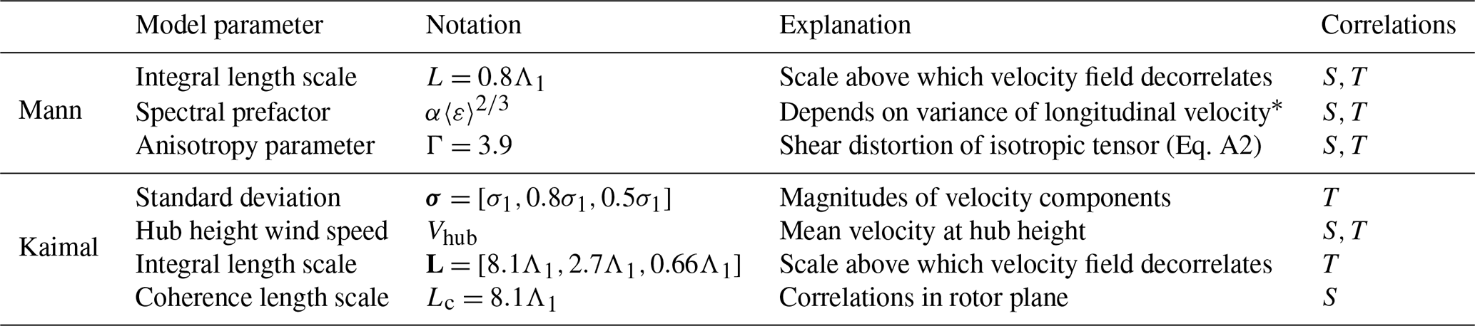
where L determines the correlation length of wind field structures, 〈ε〉 is the averaged local energy dissipation rate, and α is the Kolmogorov constant. Typically, the Mann model is fully parameterized by the correlation length L; the coefficient $\mathit{\alpha }\langle \mathit{\epsilon }{\rangle }^{\mathrm{2}/\mathrm{3}}$ of the energy spectrum, which is related to the variance of the wind field; and the non-dimensional shear parameter $\mathrm{\Gamma }=\frac{\frac{\partial U}{\partial z}L}{u}$. These parameters are further summarized in Table A1.

A2 Kaimal model of inflow turbulence

The Kaimal model exhibits several differences in the way the covariances (Eq. A1) are assembled. Firstly, unlike the Mann model, where wind field components are statistically dependent, the Kaimal model assumes the statistical independence of the components. The temporal spectral densities are thus given by

$$\begin{array}{}\text{(A4)}& \begin{array}{rl}{\widehat{C}}_{ij}\left(f\right)& =〈{\widehat{u}}_i(y,z,f){\widehat{u}}_j(y,z,-f)〉\\ & ={\mathit{\sigma }}_i^{\mathrm{2}}{\displaystyle \frac{\mathrm{4}{L}_i/V_{\mathrm{hub}}}{(\mathrm{1}+\mathrm{6}f{L}_i{)}^{\mathrm{5}/\mathrm{3}}}}{\mathit{\delta }}_{ij},\end{array}\end{array}$$

where

$$\begin{array}{}\text{(A5)}& {\widehat{u}}_i(y,z,f)=\int \mathrm{d}t{e}^{-\mathrm{2}\mathit{\pi }ift}{u}_i(y,z,t)\end{array}$$

is the single-sided Fourier transform; V_hub is the mean velocity at hub height; and $\mathit{\sigma }=[{\mathit{\sigma }}_{\mathrm{1}},{\mathit{\sigma }}_{\mathrm{2}},{\mathit{\sigma }}_{\mathrm{3}}]$ are the standard deviations and $\mathbf{L}=[L_{\mathrm{1}},L_{\mathrm{2}},L_{\mathrm{3}}]$ the integral length scales of the velocity components, which are further summarized in Table A1. Secondly, the Kaimal model considers only the effects of a mean shear profile without distortions of the covariances (Eq. A1). Moreover, the spatial coherence between two time series located at [y,z] and $[y^{\prime },z^{\prime }]$ in the rotor plane is defined according to

$$\begin{array}{}\text{(A6)}& \begin{array}{rl}{\mathit{\kappa }}_{ij}(r,f)& ={\displaystyle \frac{〈{\widehat{u}}_i(y,z,f){\widehat{u}}_j(y^{\prime },z^{\prime },-f)〉}{\sqrt{{\widehat{C}}_{ii}\left(f\right)}\sqrt{{\widehat{C}}_{jj}\left(f\right)}}}\\ & =\exp \left[-\mathrm{12}r\left({\left({\displaystyle \frac{f}{V_{\mathrm{hub}}}}\right)}^{\mathrm{2}}+{\left({\displaystyle \frac{\mathrm{0.12}}{L_{\mathrm{c}}}}\right)}^{\mathrm{2}}\right)\right]{\mathit{\delta }}_{ij},\end{array}\end{array}$$

where $r=\sqrt{(y-y^{\prime }{)}^{\mathrm{2}}+(z-z^{\prime })}$ is the separation in the rotor plane. Hence, decreasing the coherence lengths L_c implies an increased correlation between two time series i and j in the rotor plane. For further comparisons of Mann and Kaimal models in the context of offshore measurements and large-eddy simulations, we also refer the reader to Nybø et al. (2020).

Table A1 Overview of model parameters of the Mann and Kaimal models as specified by the IEC norm 61400-1 (IEC, 2019). The symbols T and S indicate whether the corresponding parameter affects the spatial correlations (S) in the rotor plane or only the temporal characteristics (T). The turbulence length scale is suggested as Λ₁=42 m. Please note that the hub height wind speed is intrinsically contained in the Mann box due to Taylor's hypothesis L_box=V_hubT. ^*Depending on the other parameters, $\mathit{\alpha }\langle \mathit{\epsilon }{\rangle }^{\mathrm{2}/\mathrm{3}}$ must be determined to yield the correct standard deviation – see Liew and Larsen (2022) discussing a target spectrum method and a target variance method to do so.