Fully coupled, high-resolution atmosphere–ocean–wave simulations of the offshore wind energy environment during Hurricane Henri (2021)

A new fully coupled modeling system, integrating atmosphere, ocean, and wave models, is presented to simulate intricate interactions during tropical cyclones and explore their potential implications for offshore infrastructure. The system is evaluated on Hurricane Henri (2021), chosen for its distinctive track along the US northeast coast, an area of densely populated regions and offshore wind energy zones. Three simulation setups are compared: atmosphere only, atmosphere–ocean, and a fully coupled atmosphere–ocean–wave model. Among them, the fully coupled model produces the most realistic results, improving not only the storm intensity near the surface but also the wind structure from the near surface to the upper atmosphere. Waves enhance ocean surface cooling with an additional 0.5 K reduction via wave-induced vertical mixing and modify wind interactions through wave-driven surface roughness. This more realistic representation of coupled heat and energy exchanges between the atmosphere and ocean yield improved wind field patterns, which are critical for comprehensive risk assessment pertaining to offshore energy infrastructures. Furthermore, the coupled system reasonably captures wind–wave misalignment during the storm, with the greatest misalignment in the left-front and rear-left quadrants, while alignment occurs on the right side of the storm due to storm motion enhancing wave growth. These spatial variations highlight the need to accurately model atmosphere–ocean–wave interactions for reliable wind load assessments.

1 Introduction

Tropical cyclones (TCs) are among the costliest and deadliest natural hazards in the US, responsible for USD 945.9 billion in damages and 6502 fatalities from 1980 to 2019 (Smith, 2020). Although track forecasts have improved over recent decades, the ability to predict TC intensity remains limited (DeMaria et al., 2014; Rappaport et al., 2009; Yamaguchi et al., 2017; Zhao et al., 2022). A key limitation lies in the incomplete representation of atmosphere–ocean interactions in models, particularly storm-induced sea surface temperature (SST) cooling (e.g., DeMaria et al., 2007; Zhao et al., 2017, 2022). This cooling is primarily driven by vertical mixing processes caused by strong TC-generated waves, intense upper-ocean shear, and upwelling associated with divergent ocean currents (Emanuel, 1986; Schade and Emanuel, 1999; Wu et al., 2016). While these air–sea interactions are recognized as critical drivers of storm intensity in a meteorological context, their implications for the offshore built environment remain insufficiently explored.

Current risk assessments conducted under hurricane conditions often simplify or omit these coupled feedback (e.g., Arthur, 2021; Chen et al., 2024; Roldán et al., 2023; Sanchez Gomez et al., 2023), potentially leading to a disconnect between state-of-the-art numerical modeling and the practical evaluation of offshore structural vulnerabilities. One critical gap in current hurricane-focused offshore wind assessments is the impact of wind–wave misalignment on structural loads and potential damage. Such misalignment can significantly increase side-to-side turbine deflections and lead to underestimations of fatigue loads by as much as 50 % in floating systems. For instance, a recent study by Shanahan and Fitzgerald (2025) found that wind–wave misalignment in floating offshore wind turbines can exceed 30° during hurricanes and reach up to ∼58° along exposed western coastal zones of Ireland. Additionally, Ma and Sun (2023) used large-eddy simulations to model the coupled wind–wave loading on fixed-bottom offshore turbines, finding that under extreme events, such as hurricanes, aerodynamic loading increases: the mean bending moment at both tower and monopile rises by ∼6 %, the standard deviation of shear force increases by up to ∼45 %, and the bending movement variability increases by ∼27 %. These findings highlight the need for dynamic, coupled modeling approaches that can capture the evolving interactions among wind, waves, and currents, especially under extreme events, such as hurricanes (e.g., Chen et al., 2013; Barr and Chen, 2024).

However, most current modeling frameworks used for wind energy risk assessment fall short in this regard. Uncoupled atmospheric models typically calculate surface roughness solely based on wind speed (e.g., via Charnock formulations; Charnock, 1955), without explicitly representing wave-induced momentum fluxes (e.g., Sanchez Gomez et al., 2023), which can bias near-surface wind fields, shear profiles, and wind veer under extreme forcing. Statistical–parametric models, while efficient for probabilistic loss estimation, represent hurricane winds using idealized radial wind profiles – such as studies that use the classic Holland model (Arthur, 2021), the two-parameter Holland formulation (Chen et al., 2024), or recent asymmetric extensions (Roldán et al., 2023). By not explicitly accounting for the evolving feedback among wind, waves, and ocean currents, these approaches can underpredict or overpredict extreme gusts and rapid directional shifts that critically drive turbine loading.

To move beyond these idealized and uncoupled approaches, this study introduces a newly developed atmosphere–ocean–wave coupled modeling system that integrates a regional atmospheric mesoscale model with ocean and surface wave models, both of which operate a high-resolution unstructured mesh. This framework, while sharing similarities with the Coupled Ocean-Atmosphere-Wave-Sediment Transport (COAWST) model (Warner et al., 2010), is distinguished by several key enhancements. First, it supports regional mesh refinement, allowing ultra-high-resolution ocean grids over targeted areas such as offshore wind farms. This feature provides more localized and detailed oceanic information, improving the system's utility for site-specific assessment. Second, our framework explicitly includes the effects of non-breaking-wave processes in the coupling system. These processes, which require custom implementation (e.g., Xu et al., 2023), are not part of the standard COAWST model but are essential for realistically representing atmosphere–ocean–wave interactions, especially under extreme wind conditions such as those associated with TCs.

Within this modeling context, the present study focuses on characterizing the coupled offshore environmental forcing rather than on turbine-level structural response. While turbine loads and wake recovery are not directly explored, the study examines key aspects of the atmosphere–ocean–wave interface that underpin such analyses. By assessing how coupling influences hub-height wind speeds and vertical wind profiles, this work provides relevant meteorological and oceanographical information that can inform future high-fidelity load modeling and offshore wind design studies and risk assessment. Accordingly, the primary objective of this study is to demonstrate the capabilities of the newly developed coupled framework and to evaluate its ability to resolve the complex atmosphere–ocean–wave processes that govern TC wind structure. We apply the system at high resolution (3 km for both atmospheric and oceanic components near the US northeast coast) to Hurricane Henri (2021) as a case study. Henri was a Category 1 storm that made landfall in Rhode Island on 22 August 2021 and traversed the offshore wind energy lease area on the northeast continental shelf. Extensive observations, including airborne Doppler radar and dropsonde data near the eyewall, enable direct evaluation of modeled fields against observations. This study represents a necessary step toward transitioning offshore wind energy assessments from idealized or uncoupled parameterizations to a fully consistent, physics-based representation of environmental forcing under extreme weather conditions.

The development of the model, including detailed information on each model component and the coupler, is described in Sect. 2. Section 3 describes the experimental design and data used for model validation using Hurricane Henri (2021) as a working example. In Sects. 4 and 5, we present results and analysis, followed by the summary and discussions in Sect. 6.

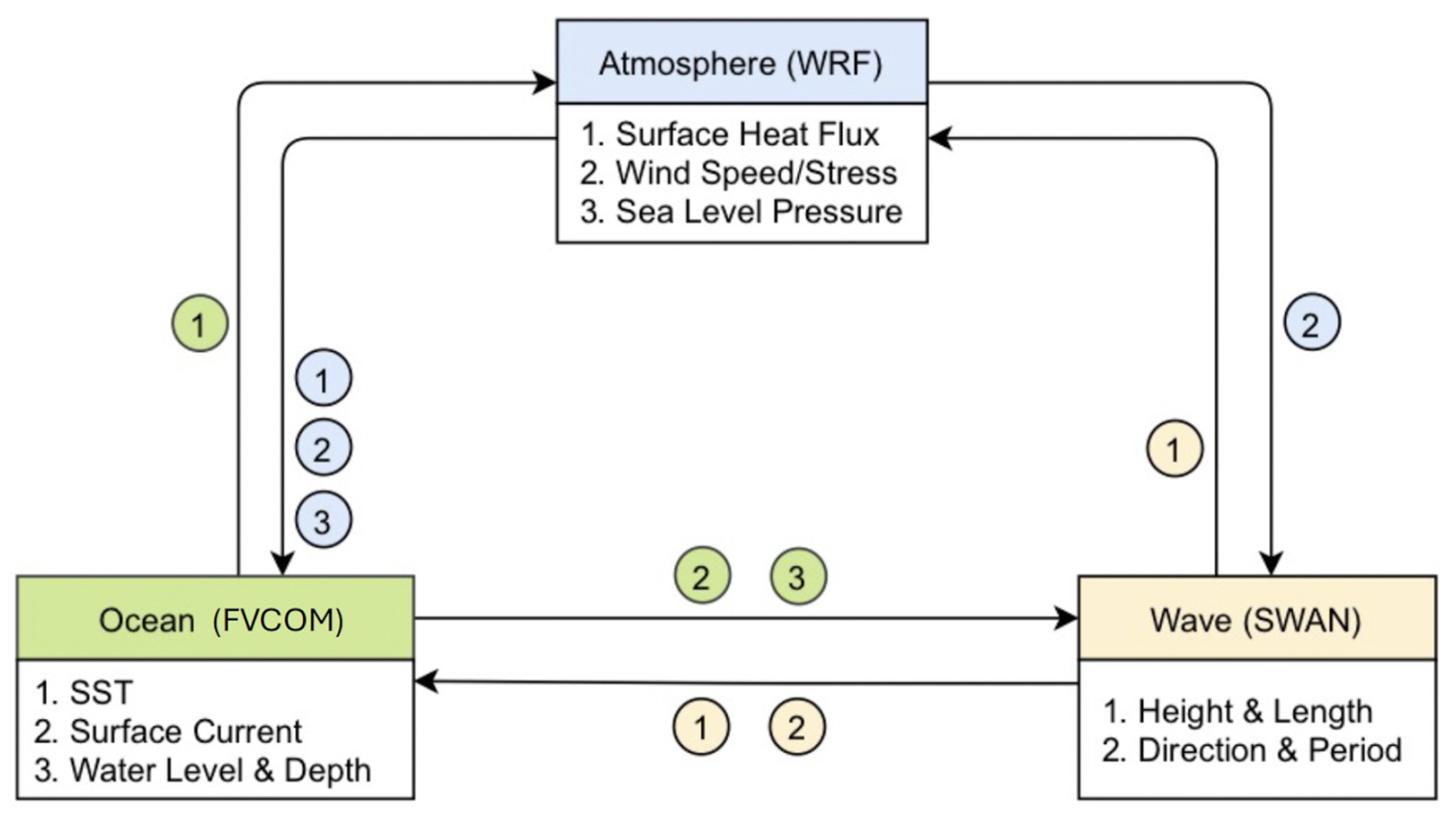
Figure 1 Schematic of the coupled atmosphere–ocean–wave system and modeling used in this study.

2 Model description

The coupled atmosphere–ocean–wave modeling system integrates three core components: the Weather Research and Forecasting (WRF) model for atmospheric processes (v4.5.1; Skamarock et al., 2019), the Finite Volume Community Ocean Model (FVCOM) for ocean circulation (v4.3.1; Chen et al., 2003, 2013), and the third-generation Simulating WAves Nearshore (SWAN) model for wave dynamics (Booij et al., 1999), with data exchanged via a coupler (Fig. 1). Hereafter, we refer to the coupled WRF-FVCOM-SWAN model as C-WFS. These components run in parallel and interact through the OASIS3-MCT coupler (Craig et al., 2017). Details on each model, recent improvements, and the coupling strategy are provided in Sect. 2.1–2.2.

2.1 Model components

WRF is a nonhydrostatic, quasi-compressible atmospheric model featuring boundary layer physics and various subgrid-scale parameterizations to simulate meso- and macroscale motions. In this study, we modified the WRF code to incorporate the wave-slope-based sea surface roughness formulation from Taylor and Yelland (2001) into several surface schemes, including MYNN (Nakanishi and Niino, 2009; Olson et al., 2019) and both the original and the revised MM5 schemes (Dyer and Hicks, 1970; Jimenez et al., 2012; Paulson, 1970; Webb, 1970):

$$\begin{array}{}\text{(1)}& Z_{\mathrm{0}}=\mathrm{1200}{H}_{\mathrm{s}}{\left({\displaystyle \frac{H_{\mathrm{s}}}{L_{\mathrm{p}}}}\right)}^{\mathrm{4.5}}+{\displaystyle \frac{\mathrm{0.11}\mathit{\upsilon }}{u_{\ast }}}{Z}_{\mathrm{0}}\le \mathrm{0.00285},\end{array}$$

where Z₀ is the surface roughness length, H_s is the significant wave height, L_p is the wavelength at the peak of the spectrum, υ is kinematic viscosity, and u_∗ is the friction velocity. Although C-WFS includes alternative wave-based formulations (e.g., Drennan et al., 2003, 2005), our tests showed that the capped Taylor and Yelland (2001) method yielded the optimal performance for our case study.

The ocean component, FVCOM (v4.3.1), is a 3D, free-surface, prognostic coastal circulation model that solves the primitive equations on an unstructured triangular grid using the finite-volume method. It enables dynamic interaction between ocean and atmospheric conditions throughout the simulation. In this study, we modified FVCOM to include vertical mixing induced by non-breaking waves by adding a wave-related term to the turbulence eddy diffusivity B_υ, following Ghantous and Babanin (2014a, b) and Aijaz et al. (2017):

$$\begin{array}{}\text{(2)}& B_{\mathit{\upsilon }}=\mathit{\alpha }{A}^{\mathrm{3}}\mathit{\kappa }\mathit{\sigma }{e}^{\mathrm{3}\mathit{\kappa }z},\end{array}$$

where α=0.1, A is the wave amplitude ($H_{\mathrm{s}}/\mathrm{2}$), κ is the wave number (2$\mathit{\pi }/L$), σ is the peak wave frequency ($\mathrm{1}/T_{\mathrm{p}}$), and z is water depth.

The wave model component, SWAN v41.01, is a third-generation spectral wave model developed at Delft University of Technology that computes random, short-crested wind-generated waves in coastal regions and inland waters (http://swanmodel.sourceforge.net/, last access: 1 April 2026). It solves the evolution equation of wave action density in space time, frequency, and wave direction dimensions (Pringle and Kotamarthi, 2021). Various wave energy sources and sinks are modeled, including wave generation by wind, wave decay due to whitecapping, bottom friction, depth-induced wave breaking, and energy redistribution through nonlinear wind–wave interactions.

2.2 Coupler and coupling

OASIS3-MCT is a parallel coupler that synchronizes 2D and 3D field exchanges. Figure 1 outlines the C-WFS coupling framework and exchanged variables. WRF provides FVCOM with surface forcing – including friction velocity, winds, sea level pressure, heat fluxes, and radiation fluxes – while receiving SST from FVCOM as over-ocean boundary conditions. WRF also supplies wind fields to SWAN for wave simulations. In return, SWAN sends significant wave height and peak wavelength to WRF, which uses them to calculate sea surface roughness based on Eq. (1). FVCOM uses wave fields from SWAN to compute radiation stress gradients, Stokes velocities, wave-enhanced bottom stresses, and non-breaking-wave-induced mixing; breaking wave mixing is included via stress gradients. FVCOM also provides surface currents to SWAN, enabling Doppler shift effects from currents on wave behavior. This integrated coupling improves wave prediction accuracy by capturing wave–current interactions more realistically.

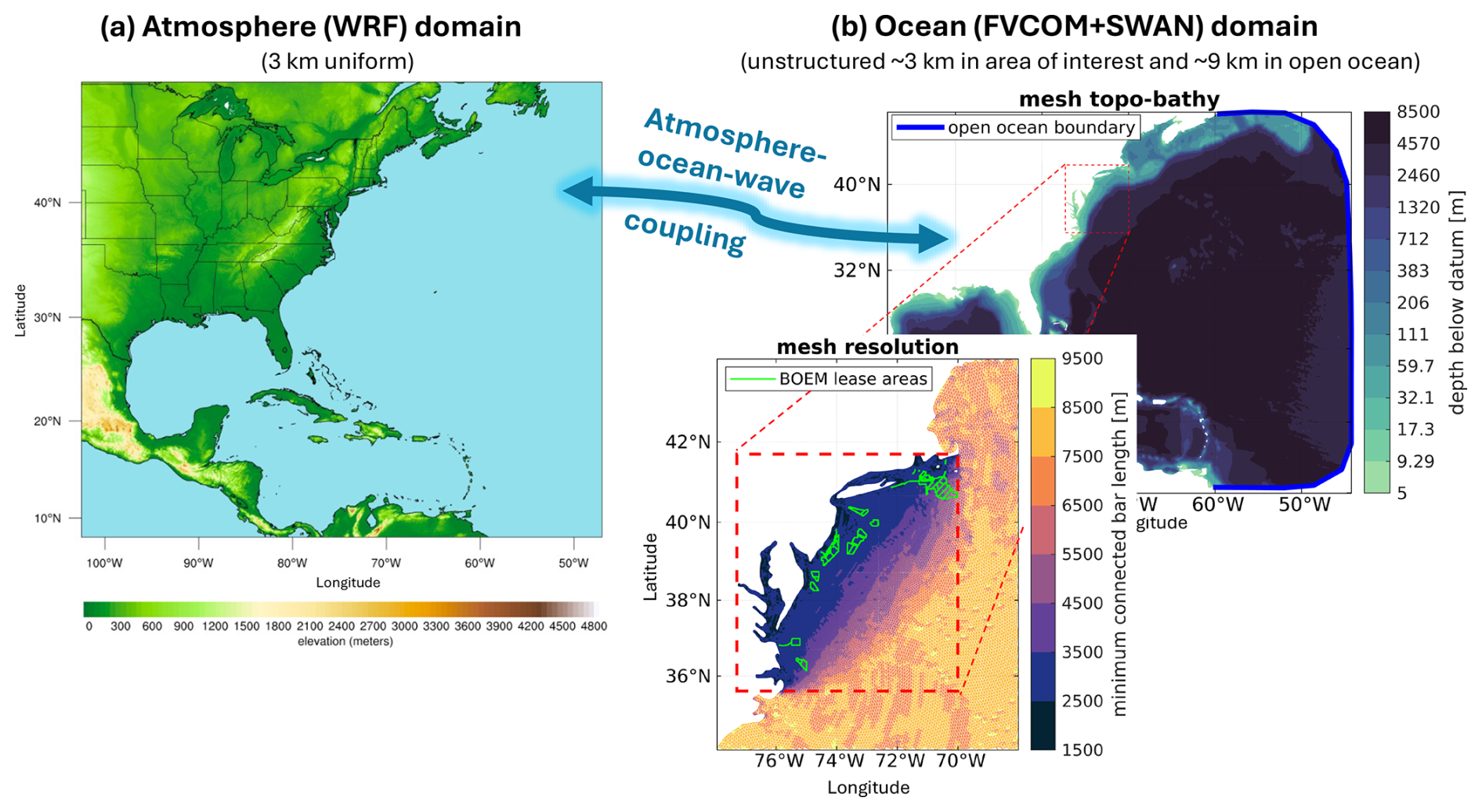
Figure 2 (a) WRF model domain with terrain height elevation and (b) FVCOM and SWAN domain with bathymetric depths and a zoomed-in view to the refined mesh grid along the northern US East Coast and BOEM offshore lease areas.

3 Application of C-WFS modeling system

3.1 Experimental design and configuration

To evaluate the integrated impact of ocean and wave processes on TC simulations, three experiments were performed. Experiment “A” (atmosphere only) uses WRF with a 6-hourly updated SST. “AO” couples WRF with FVCOM, enabling atmosphere–ocean interaction but no wave effects. “AOW” fully couples WRF, FVCOM, and SWAN via OASIS3-MCT, allowing hourly, multi-way atmosphere–ocean–wave exchanges.

WRF is configured with a 3 km horizontal resolution and 46 vertical levels (12 below 100 m), covering much of the North Atlantic Basin (Fig. 2a). It uses 6-hourly 0.25° National Centers for Environmental Prediction (NCEP) Global Forecast System (GFS; NCEP, 2015) analysis data for atmospheric initial and boundary conditions, with SSTs prescribed from GFS in “A”. The model employs WSM6 microphysics (Hong and Lim, 2006), RRTMG radiation (Iacono et al., 2008), Yonsei University PBL (Hong et al., 2006), and the Eta similarity surface layer scheme (Jimenez et al., 2012). No cumulus parameterization is used, as 4 km resolution or less supports convection-permitting simulations (Akinsanola et al., 2024; Kouadio et al., 2020; Qing and Wang, 2021; Sun et al., 2016).

The ocean domain (FVCOM) covers most of the WRF domain, with horizontal resolution ranging from ∼9 km in the open ocean to ∼3 km over the continental shelf. It uses 40σ vertical layers to capture steep coastal bathymetry. Vertical mixing processes are simulated using the Mellor–Yamada level-2.5 (MY25) turbulence closure model (Mellor and Yamada, 1982), and horizontal diffusivity is computed using the Smagorinsky numerical formulation (Smagorinsky, 1963). Initial and boundary conditions for currents, temperature, salinity, and water level are provided by $\mathrm{1}/\mathrm{12}$° Hybrid Coordinate Ocean Model (HYCOM) analysis data (Cummings and Smedstad, 2014).

The wave model domain matches the FVCOM domain, using ∼12 km horizontal resolution. The wave spectrum is divided into 36 directional and 24 frequency bins (0.04–1 Hz). Wave physics include Komen et al. (1984) for growth and whitecapping, Madsen et al. (1988) for bottom friction, and a constant depth-limiting breaker index, all with default settings. Swell boundary conditions are omitted due to minimal impact at the eastern boundary, and the model is initialized from a quiescent state.

All experiments were initialized at 18:00 UTC on 19 August 2021 and simulated for 102 h. Nudging techniques were intentionally omitted to better isolate the effects of atmosphere–ocean–wave coupling on TC characteristics. Additional tests using various physics schemes and forcing datasets (e.g., ERA5) confirmed the robustness and low sensitivity of the results to model configuration choices, although the supporting results are not presented in this paper.

3.2 Method and data

Model results are evaluated against several observational datasets, including the International Best Track Archive for Climate Stewardship (IBTrACS; Knapp et al., 2010) – which provides TC position, minimum sea level pressure (SLP), and maximum 10 m sustained winds at ∼6 h intervals – and airborne observations. The airborne data include the Tropical Cyclone Radar Archive of Doppler Analyses with Recentering (TC-RADAR; Fischer et al., 2022) and dropsondes from NOAA's Hurricane Research Division. TC-RADAR contains X-band Doppler radar data from NOAA's WP-3D aircraft, scanning in the front and back directions to produce detailed 3D analyses of the TC inner-core structure. Each mission typically includes three to four center passes, with storm-centered “recentering” techniques used to generate gridded analyses. Our simulations adopt the same storm-centered coordinates for direct comparison. A 300 km × 300 km grid is centered on the grid cell with minimum SLP in each dataset. To fill the 0–0.5 km altitude gap not captured by radar, we include dropsonde data. Due to slight differences in storm track and speed between the model and observations (Fig. 3), dropsonde positions are adjusted relative to the storm center (e.g., Creasey and Elsberry, 2017). Seven dropsondes (shown in Fig. 3d) from a single flight across the storm center were selected for evaluation; this flight crossed the storm from east to west within 50 min from 23:21 UTC on 21 to 00:11 UTC on 22 August 2020 (with exact times indicated in Fig. 3d), 12 h before peak intensity.

Modeled ocean surface waves are compared with observations from two National Data Buoy Center buoys (NDBC, 2008), 41001 and 41002, located on the left of the storm track on the continental slope. While there are more buoy locations, our focus is on the variation in storm-induced winds and waves along Henri's track. We exclude stations near the US northeast coast due to the models' track bias after 22 August (more discussion in Sect. 4). The buoy data provide surface wind and wave information, including surface wind speed, significant wave height, and peak wave period and direction. In addition to in situ NDBC buoy measurements, we compiled a series of daily SST data from the Operational Sea Surface Temperature and Ice Analysis (OSTIA) system (Good et al., 2020) at 0.05° × 0.05° resolution to determine the pre- and post-storm environment as well as the difference between them.

The radius of maximum wind (RMW) defines the location of the maximum winds in a TC and is critical to understanding intensity change and hazard impacts. In this study, we azimuthally average the vertical profiles of the seven dropsondes and the simulations of wind speed relative to RMW to define the areas within and beyond the eyewall, allowing for a detailed comparison of the storm's inner- and outer-core regions.

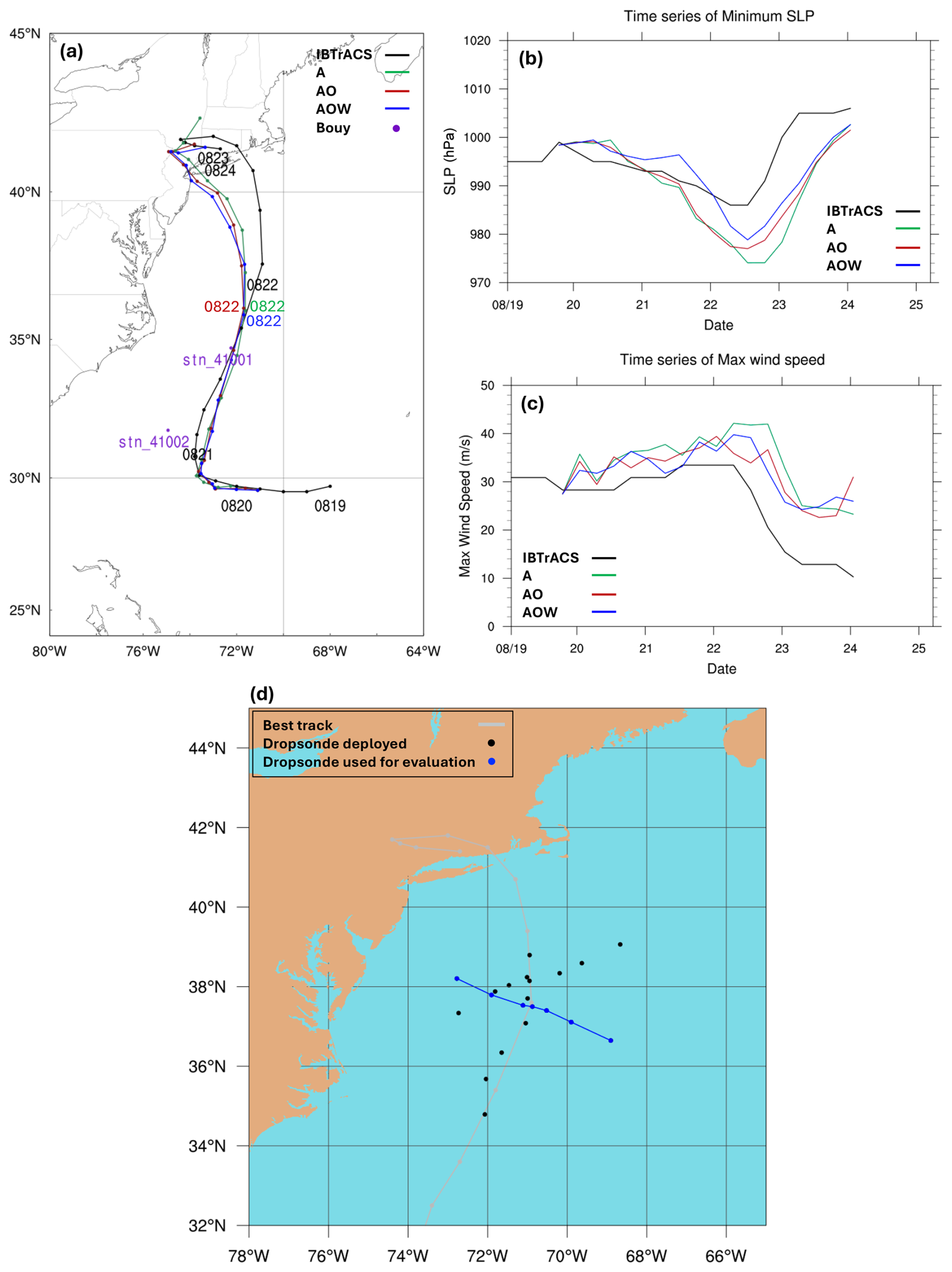
Figure 3 Comparison of simulated (a) track, (b) minimum sea-level pressure (SLP), and (c) maximum 10 m wind speed of Hurricane Henri with IBTrACS Best Track data from 18:00 UTC on 19 to 00:00 UTC on 24 August 2021. The black lines show IBTrACS data; the green, red, and blue lines represent experiments “A”, “AO”, and “AOW”, respectively. Panel (d) shows the IBTrACS track (grey) with dropsonde positions (black and blue dots). The seven dropsondes, shown as blue dots, were released during a single NOAA WP-3D flight that traversed the storm center from west to east over approximately 50 min (23:21 UTC on 21 to 00:11 UTC on 22 August). These dropsondes were used to evaluate model performance. The purple dots in (a) denote buoy stations 41001 and 41002 from the National Data Buoy Center.

4 Model validation

4.1 Track and intensity

Figure 3 presents the tracks, SLP minima, and surface wind speed maxima derived from the three simulations alongside IBTrACS. We emphasize at the outset that the purpose of this evaluation is not to assess forecast skill, but to provide a baseline comparison that enables interpretation of how atmosphere–ocean–wave coupling alters storm evolution and wind structure relative to partially coupled or uncoupled configurations.

The results indicate that variations in Henri's tracks across the three experiments show only minor differences (Fig. 3), consistent with previous findings suggesting that TC tracks are predominantly controlled by large-scale atmospheric circulation processes, rather than by atmosphere–ocean interactions at the temporal and spatial scales resolved in these models (e.g., Zambon et al., 2014). The root mean square error (RMSE; Table 1) of position indicates that all three simulations have similar track errors, with values of 123.7 km for “A”, 119.4 km for “AO”, and 126.1 km for “AOW”. Higher errors stem mainly from deviations after 00:00 UTC on 22 August, likely due to biases in midlatitude upper-level wave patterns (e.g., troughs and ridges) affecting the storm embedded in the baroclinic zone. While preliminary sensitivity tests indicate that spectral nudging can reduce track errors, nudging is intentionally excluded here to avoid constraining storm evolution and to better isolate the physical effects of atmosphere–ocean–wave interactions. All subsequent analyses therefore reflect unconstrained results.

In contrast to track, all three experiments overestimate storm intensity in terms of minimum SLP throughout most of Henri's lifecycle (Fig. 3b), particularly near peak at 12:00 UTC on 22 August. Nevertheless, systematic differences emerge among the experiments. Both ocean-coupled simulations (“AO” and “AOW”) reduce the magnitude of SLP overestimation relative to “A”. In “AOW”, the overestimation of minimum SLP is delayed until 00:00 UTC on 22 August, after which it reaches the weakest peak minimum SLP among the three. This results in the lowest RMSE in minimum SLP (Table 1). These temporal trends also apply to the maximum surface wind speed (Fig. 3c and Table 1), demonstrating a reduction in overestimation of maximum surface wind speed in both “AO” and “AOW” compared to “A”. Between experiments “AO” and “AOW”, while “AOW” generally exhibits weaker wind speeds compared to “AO”, they become stronger as the storm approaches and reaches its peak intensity, in contrast to the findings for minimum SLP. This apparent decoupling between these two intensity metrics highlights the role of wave-modulated surface roughness and air–sea momentum exchange, and it motivates the mechanistic analysis presented in Sect. 5.

Overall, while the simulations exhibit clear deficiencies in rack and intensity, the consistent and systematic differences among “A”, “AO”, and “AOW” provide a useful framework for diagnosing how coupled ocean and wave processes influence storm structure. These relative differences – rather than absolute forecast accuracy – form the basis for the process-oriented analysis that follows.

Table 1 Root mean square error (RMSE) for each simulation in terms of minimum sea level pressure (hPa), maximum surface wind speed (m s⁻¹), and cyclone track (km).

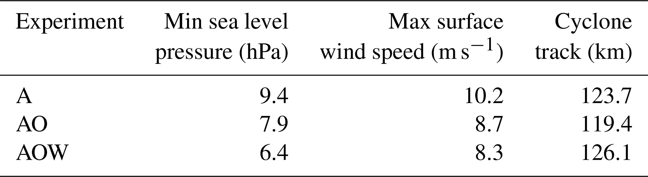
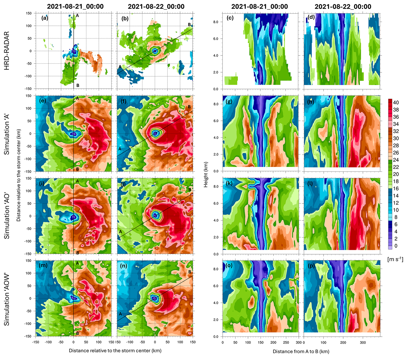
Figure 4 NOAA WP-3D airborne Doppler radar (TC-RADAR) wind speeds at the 1 km level are shown in the top row, with model-simulated wind speeds from the “A” (second row), “AO” (third row), and “AOW” (fourth row) simulations of Hurricane Henri (2021) at 00:00 UTC on 21 (first and third columns) and 22 August (second and fourth columns). Vertical cross-sections along the A–B line (marked in the left two panels) are shown in the right two columns. All horizontal fields are plotted in a 300×300 km storm-centered domain.

4.2 Storm wind structure

Figure 4a–d show 1 km level wind speeds and vertical profiles from TC-RADAR at 00:00 UTC on 21 and 22 August 2021, along the black lines in Fig. 4a–b. On 21 August, observations reveal a strongly asymmetric wind field, with the highest winds concentrated on the storm's right side. This asymmetry results from the combination of Henri's cyclonic circulation and its poleward motion, which enhances wind speeds on the right through additive forward momentum. The vertical cross-section (Fig. 4c) along line A–B shows wind speeds >20 m s⁻¹ largely confined below 4 km on the southern side but extending to 8 km on the northern side. By 00:00 UTC on 22 August, 12 h before its minimum central pressure, Henri's wind field becomes more symmetric and compact, with a closed eyewall and winds exceeding 24 m s⁻¹ (Fig. 4b, d). A clear calm zone is evident within the eyewall, extending up to 9 km. Strong winds are more evenly distributed around the center but remain the strongest on the right. Corresponding model-simulated wind profiles and 1 km level horizontal wind fields at both times are shown in Fig. 4e–p.

All three simulated storms capture Henri's structural evolution reasonably well – from a broad, asymmetric wind pattern with strong right-side winds at 00:00 UTC on 21 August (as seen in TC-RADAR) to a more compact, symmetric structure by 00:00 UTC on 22 August. However, the simulations, especially experiments “A” and “AO”, overestimate wind intensity both horizontally and vertically. The fully coupled run “AOW” reduces this bias, producing more realistic radial wind profiles at 1 km along line A–B (Fig. S1 in the Supplement) and achieving the highest Pearson correlations with TC-RADAR (r=0.95 for horizontal distribution and 0.72 for vertical cross-section). To assess wind distribution more comprehensively, we use probability density functions (PDFs) across all available TC-RADAR grid cells (0.5–9 km altitude within a 300×300 km domain centered on the storm). All simulations skew toward higher wind intensities, but “AOW” shows improved performance, especially in the upper tail, suggesting reduced wind bias during storm intensification (Fig. 5).

While TC-RADAR provides rich horizontal and vertical coverage, it only samples above 0.5 km, limiting surface-level validation. Dropsonde data help bridge this gap. Figure S2 shows vertical cross-sections up to an altitude of 3.2 km along the blue line in Fig. 3d: consistent with TC-RADAR, the strongest winds appear 10–30 km east of the center, while much weaker winds dominate the western side. These asymmetries are captured in all simulations, although they are generally overestimated.

Azimuthally averaged vertical profiles (Fig. 6) in the inner-eyewall ($\mathrm{0.2}\le r/\text{RMW}\le \mathrm{1}$) and outer-eyewall ($\mathrm{2}\le r/\text{RMW}\le \mathrm{2.5}$) regions at the dropsonde locations further confirm that all simulations overestimate low-level winds (below 2 km). However, “AOW” aligns more closely with observations, particularly in the outer eyewall. This improvement is critical, as it provides the necessary baseline environmental forcing for offshore wind energy studies, including high-fidelity load modeling and risk assessment in storm-prone regions.

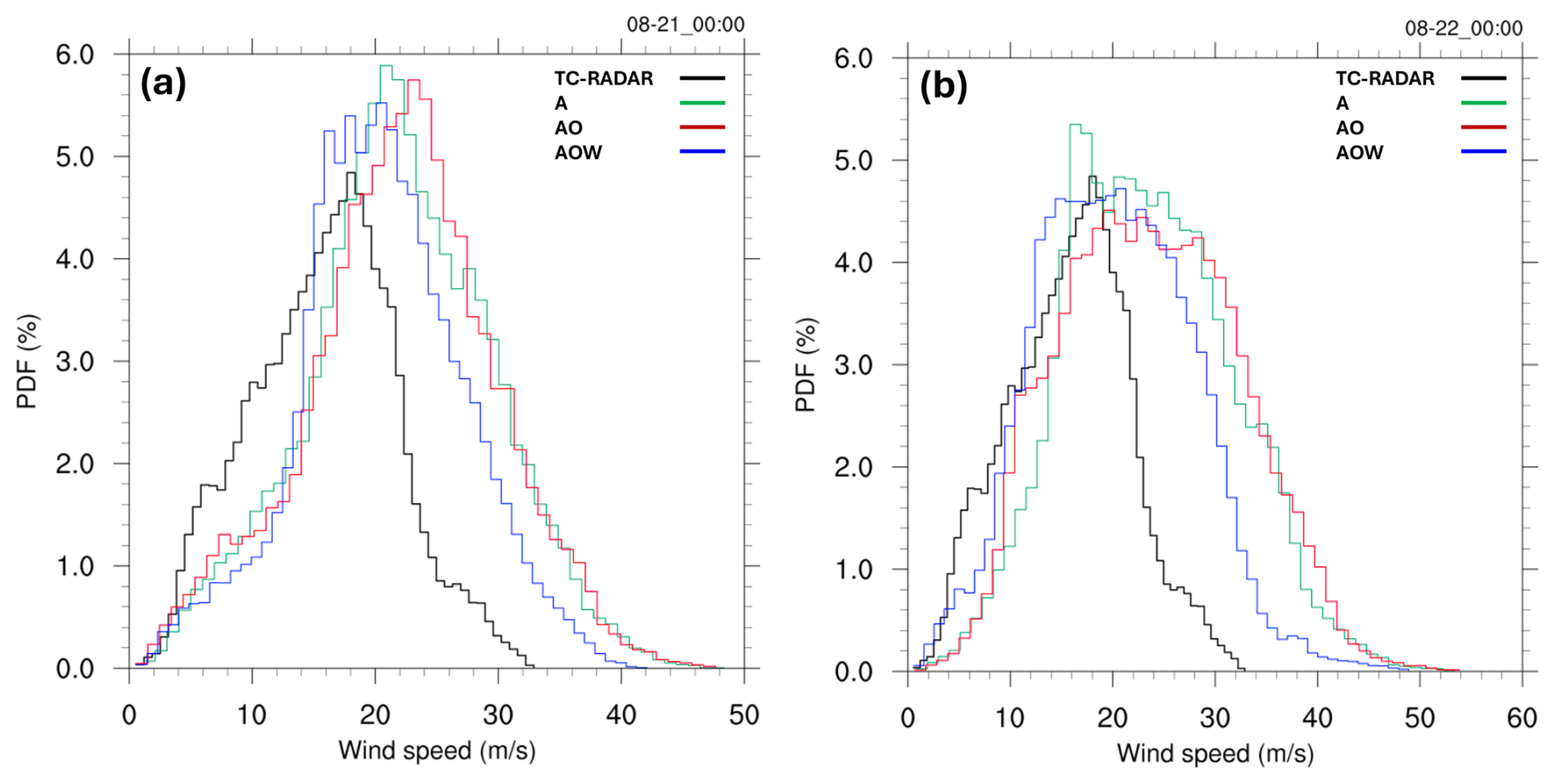
Figure 5 Probability density function of wind speed in a 300 km × 300 km storm-centered coordinate, considering vertical levels from 0.5 to 9 km above the ground, for 00:00 UTC on 21 August (a) and 22 August (b) 2021. The data are derived from TC-RADAR (black lines), experiment “A” (green lines), experiment “AO” (red lines), and experiment “AOW” (blue lines).

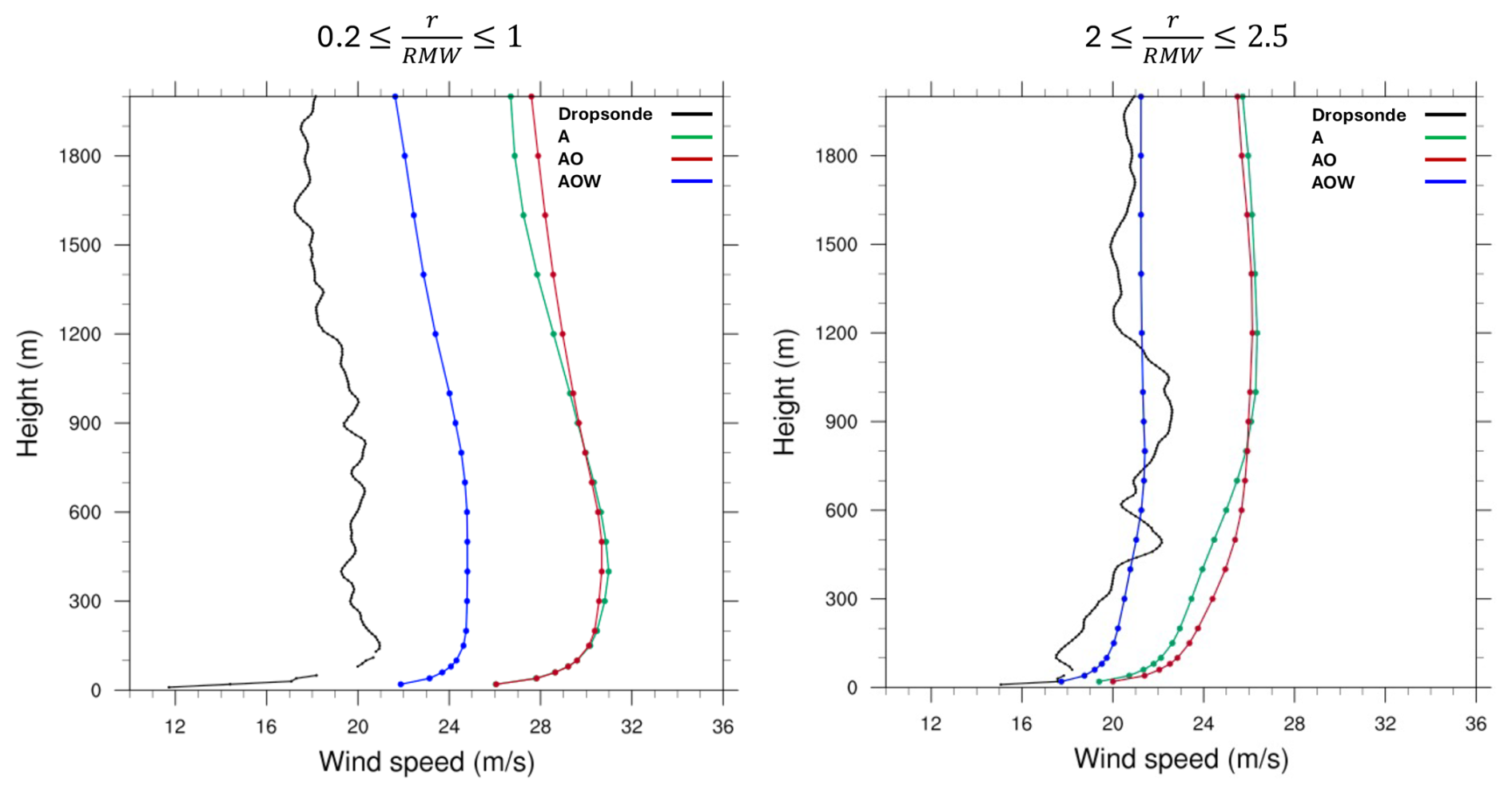
Figure 6 Vertical profiles of azimuthally averaged wind speed for dropsondes (black lines), experiment “A” (green lines), experiment “AO” (red lines), and experiment “AOW” (blue lines). The vertical profiles are azimuthally averaged in the inner-eyewall region (left; $\mathrm{0.2}\le r/\text{RMW}\le \mathrm{1}$) and the outer-eyewall regions (right; $\mathrm{2}\le r/\text{RMW}\le \mathrm{2.5}$), based on the locations of the seven dropsondes highlighted with the blue dots in Fig. 3d at 00:00 UTC on 22 August 2021. RMW indicates the radius of maximum wind, and r shows the radius relative to the storm center.

4.3 Sea surface temperature

From the ocean's perspective, SST and surface roughness are key factors influencing TC intensity, as they directly affect the exchange of heat, moisture, and momentum between the ocean and the storm (Zambon et al., 2014, 2021; Zhao et al., 2022). The main distinction among the three simulations lies in how SST and ocean surface roughness are represented, influencing surface enthalpy and momentum fluxes through air–sea interactions. Accordingly, SST is used both as an indicator of storm evolution and as a dynamic driver of intensity across the three simulations. Therefore, evaluating how well the coupled model reproduces observed SST is critical for assessing its ability to realistically capture ocean dynamics and storm–ocean interactions.

Figure 7 shows the SST distribution across the simulation domain for all three experiments, along with OSTIA observations from 12:00 UTC on 20 August to 12:00 UTC on 23 August 2020. Since OSTIA provides daily SST data, the statistics in Table 2 represent an average over these 4 d. In experiment “A”, the SST is derived from GFS and is technically driven by observed SST data. Therefore, it captures key large-scale features well, such as the Gulf Stream and warm waters along the Gulf Coast. However, it consistently underestimates SST across the domain during this period. In addition, its relatively low resolution (0.25°) limits its ability to capture small-scale SST patterns, contributing to the higher RMSE values shown in Table 2.

The ocean-coupled simulations (“AO” and “AOW”), which are driven by oceanic initial and boundary conditions from the HYCOM analysis, successfully capture major SST features such as the Gulf Stream and Gulf Coast, with enhanced spatial detail. This improved representation contributes to lower RMSE values compared to the atmosphere-only simulation (“A”) (Table 2). However, both “AO” and “AOW” tend to overestimate SSTs in the open North Atlantic and underestimate them near the northeastern US coast (Fig. 7d, l, p), likely due to cold wakes generated by the simulated storms and deviations in their tracks from observations. Nevertheless, the ocean-coupled simulations reproduce the observed SST reasonably well, with RMSE values of 0.564 and 0.577 for “AO” and “AOW”, respectively – lower than that of “A” – while maintaining comparable pattern correlation overall (Table 2).

To assess the potential influence of track biases on SST and MSLP, we first examined “A” simulation. It exhibits overintensification of MSLP, a consequence of its simulated track failing to coincide with the observed cold wakes in the GFS data. This misalignment prevents the realistic capture of crucial atmosphere–ocean heat and moisture exchanges. Conversely, ocean-coupled simulations (“AO” and “AOW”) more accurately represent storm-induced modifications to surface energy and momentum fluxes. By explicitly modeling SST cooling along their simulated storm paths, these coupled runs achieve a more realistic depiction of storm intensity. In particular, the “AOW” simulation shows enhanced SST cooling around the time of peak intensity and thereafter, further contributing to a reduction in MSLP. Spatial and temporal averaging of SST within a 300 km × 300 km storm-centered domain from 12:00 UTC on 21 August to 12:00 UTC on 22 August indicates an SST of 299.7 K for “AOW” compared to 300.2 K previously – representing a 0.5 K reduction and bringing it closer to the OSTIA value of 299.1 K (Table 3). Details of the storm-centered SST distributions are provided in the Supplement (Fig. S3). This improved performance in “AOW” can be attributed to the effect of wave-induced vertical mixing, which effectively brings cooler subsurface water to the surface, aligning with our previous discussion and prior research (e.g., Wada and Usui, 2010; Zambon et al., 2014).

Table 2 Temporally averaged root mean square error (RMSE) and Pearson product-moment coefficient of linear correlation (r) for SST in each simulation compared to OSTIA SST observations from 12:00 UTC on 20 August to 12:00 UTC on 23 August 2021.

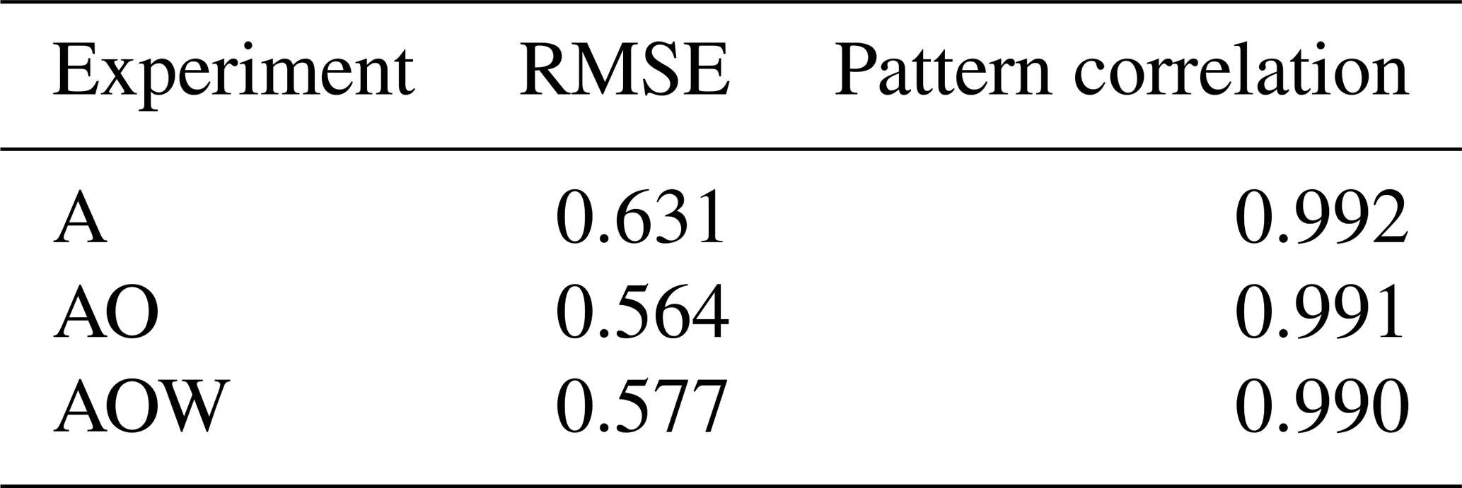
Table 3 Spatially averaged SST (K) derived from A, AO, AOW, and OSTIA observations in a 300 km × 300 km storm-centered coordinate at 12:00 UTC on 20 August, 12:00 UTC on 21 August, and 12:00 UTC on 22 August.

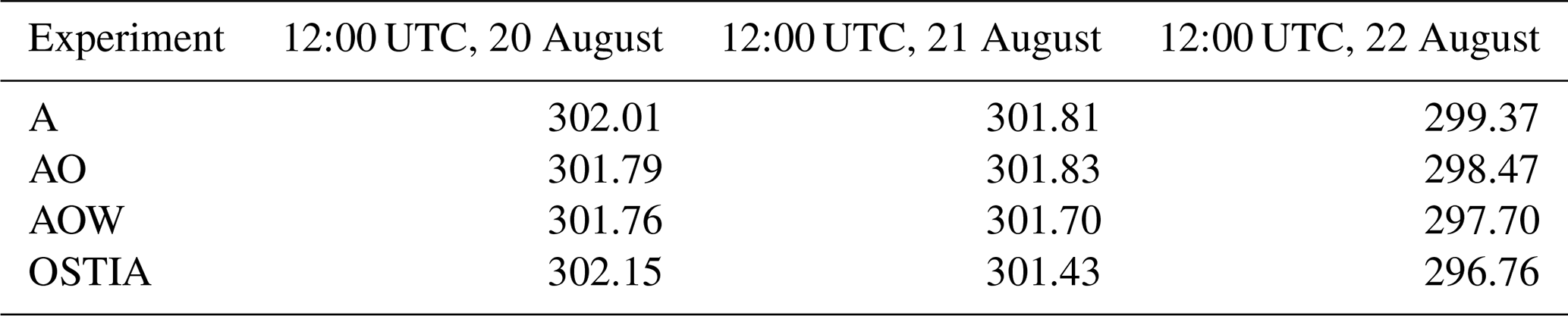
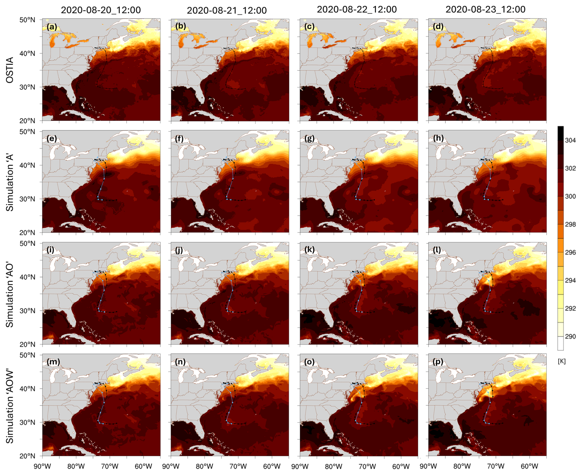
Figure 7 SST distribution (K) for OSTIA (top row), “A” (second row), “AO” (third row), and “AOW” (bottom row) at 12:00 UTC on 20 August (first column), 21 August (second column), 22 August (third column), and 24 August 2020 (fourth column). The black dots and lines indicate the best track derived from IBTrACS. The light blue dots and lines depict simulated storm locations and tracks.

4.4 Ocean surface waves

This section assesses how accurately our model simulates ocean surface waves during Hurricane Henri at two NDBC buoy locations. During Henri's primary development, buoy 41001 was directly in the path of the eyewall, while buoy 41002 was positioned approximately 120 km to the left of the storm's center during its earlier stages (Fig. 3a). The fully coupled experiment successfully captures the general temporal trends in wind speed at both sites (Fig. 8a–b). However, a slower simulated storm translation speed, particularly between 06:00 and 12:00 UTC on 21 August, led to a delay of roughly 12 h in both wind speed and wave height peaks. Furthermore, the model overestimates significant wave height by about 1–2.5 m at both locations during peak conditions (Fig. 8c–d). At station 41001, this overestimation is primarily attributable to discrepancies in wind speed. For station 41002, an additional contributing factor is the model's faster simulated translation speed – 6.3 m s⁻¹ compared to the observed 4.8 m s⁻¹ between 00:00 and 06:00 UTC on 21 August. It is well-established that increased forward motion enhances wind speed and wave growth on a storm's right side, leading to higher waves (Chen et al., 2013). While the model accurately reproduces wave direction at station 41001, it fails to capture the sharp directional shift observed at station 41002 between 06:00 and 09:00 UTC on 21 August (Fig. 8e–f). This discrepancy may stem from the model's increased wave height and wavelength, which can suppress rapid directional changes. Despite these biases in wave height magnitude and timing, the model generally provides a reasonable representation of wave behavior at both locations and successfully captures key trends in storm-induced wave dynamics during Hurricane Henri.

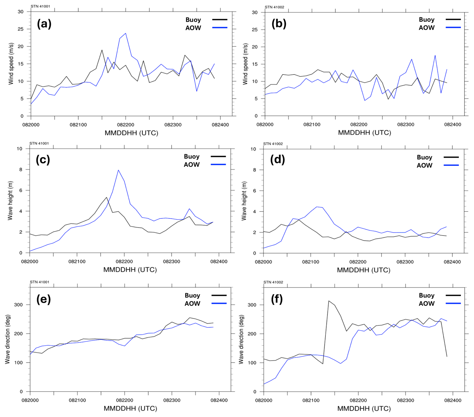
Figure 8 Comparison of the “AOW” simulation (blue) with observations (black) for Hurricane Henri from 00:00 UTC on 20 August to 00:00 UTC on 24 August 2021: (a–b) wind speed (m s⁻¹), (c–d) significant wave height (m), and (e–f) wave direction. The right column shows data from station 41001, while the left column depicts data from station 41002. The locations of stations 41001 and 41002 are shown in Fig. 3a.

Understanding the accuracy of modeled ocean surface waves, particularly their directional characteristics, is crucial because previous investigations into TC wind impacts on offshore wind turbines (e.g., Sanchez Gomez et al., 2023; Wei et al., 2017; Itiki et al., 2023) have often relied on atmosphere-only frameworks or empirical wave representations. As noted in several of those studies, such approaches necessarily simplify or exclude explicit wind–ocean–wave coupling processes, which may influence both direct and indirect load pathways. These acknowledged modeling limitations motivate the need for coupled approaches that better represent wind–wave interactions when assessing offshore wind risk extreme conditions. For instance, Ma and Sun (2023) demonstrated that under extreme wind–wave conditions, such as those in hurricanes, coupling between wind and wave dynamics significantly increases the aerodynamic loads on offshore wind turbines. This coupling markedly amplifies the variability of those loads, suggesting that traditional decoupled models may underestimate the structural demands during such severe events.

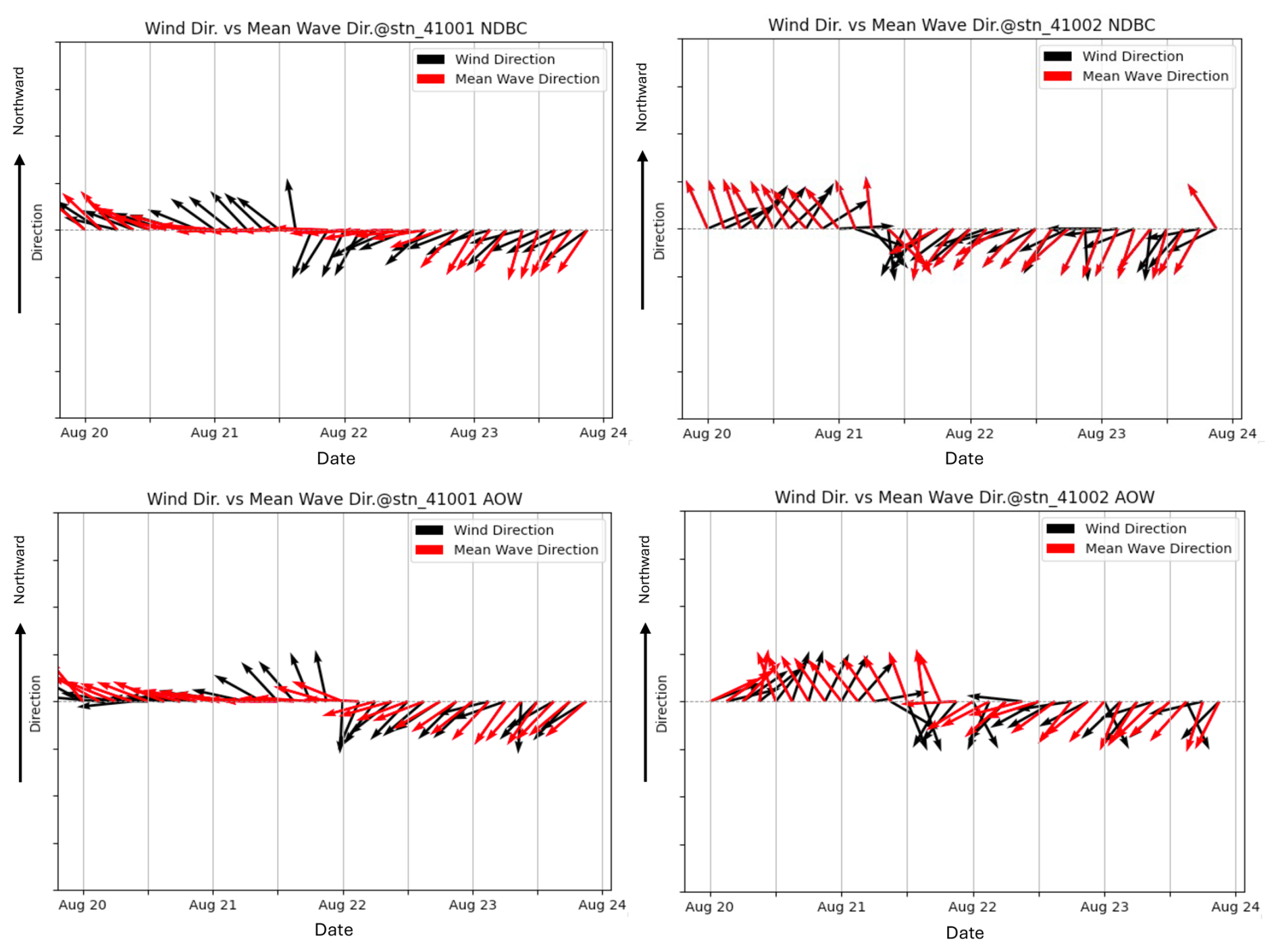
Figure 9 Time series comparison of surface wind direction and mean ocean surface wave direction at two NDBC buoy stations, 41001 (left column) and 41002 (right column), derived from NDBC buoys (top panel) and experiment “AOW” (bottom panel).

Figure 9 shows that wind and wave alignment varies considerably over time, with periods of near co-alignment interspersed with misalignments. The directional divergence is site-specific, highlighting the influence of localized impact depending on locations relative to the storm center. “AOW” captures key characteristics of directional interactions, reproducing the timing and magnitude of misalignment trends reasonably well (Fig. 9, bottom panel). Notably, the simulations capture the directional sensitivity at both sites, suggesting fidelity in representing storm-induced wave generation and propagation. By resolving wind–wave misalignment, the fully coupled modeling system provides a more physically consistent description of the environmental conditions relevant to offshore infrastructure under extreme events such as TCs.

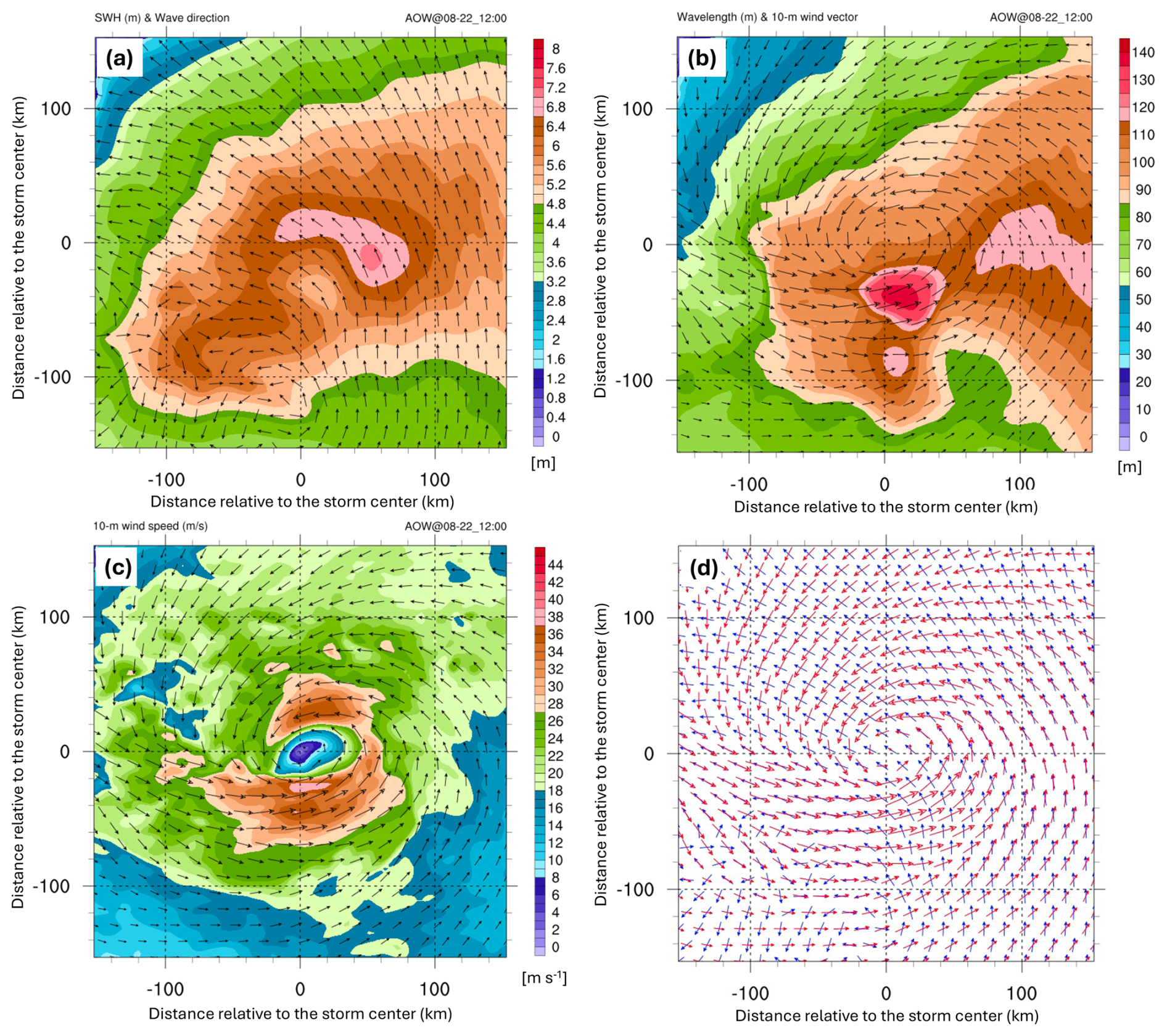
Figure 10 The fully coupled model output at 12:00 UTC on 22 August 2021 includes (a) significant wave height (shaded; in meters) and wave direction, (b) mean wavelength (shaded; in meters) and 10 m wind, (c) 10 m wind speed (shaded; in m s⁻¹) and vectors, and (d) wave (blue) and wind (red) vectors. All plots are in a 300×300 km storm-centered domain, with a 20 m s⁻¹ reference wind vector shown in panels (b) and (c).

Figure 10 illustrates simulated ocean surface wave conditions and 10 m wind vectors from the “AOW” experiment at 12:00 UTC on 22 August. Consistent with prior studies (e.g., Chen et al., 2013; Wright et al., 2001), TC-induced wave fields typically exhibit asymmetry, with the highest significant wave heights occurring in the front-right quadrant. This pattern is clearly evident in our simulation, as Henri moves northwest, producing the largest waves in its right and front-right quadrants (Fig. 10a). The storm's motion further enhances wave growth on the right side due to a longer fetch (Fig. 10a–b). Significantly, directional misalignment between wind and waves is apparent across most storm quadrants, except on the right side where both wind and waves are aligned, also consistent with previous findings (Fig. 10d). This widespread misalignment and aligned directions highlight the complex atmosphere–wave interactions that necessitate careful consideration in offshore wind load assessments.

5 Mechanisms underlying the improvement in the fully coupled experiment

Compared to experiments “A” and “AO”, “AOW” reduces the overestimation of storm intensity (minimum SLP; Fig. 3) and improves the storm-scale wind structure (Fig. 4), PDF distribution (Fig. 5), and profiles (Fig. 6) from the near surface to the upper troposphere. To understand these improvements, we analyze SST and surface enthalpy fluxes in “AOW” versus “AO” to assess the role of wave-induced processes in Henri's evolution. Experiment “A” is excluded since it is atmosphere only and lacks atmosphere–ocean interactions.

Because “AO” and “AOW” have very similar storm tracks and translation speeds, we can isolate surface processes – SST, enthalpy flux, and surface roughness length (Z₀) – to evaluate their impact on storm intensity and evolution. In “AOW”, ocean surface waves affect Z₀, which regulates momentum, heat, and moisture exchange at the air–sea interface. In uncoupled simulations like “AO”, Z₀ follows Charnock's formulation and depends only on wind speed, with no explicit dependence on wave-state properties. This limits capturing dynamic air–sea interactions during TCs, where sea state significantly influences momentum transfer and storm development. Focusing on 12:00 UTC, 22 August – about 12 h before landfall when both simulations reach peak minimum SLP – reveals notable differences in Z₀ distribution (Fig. 11). In “AO”, the distribution and strength of Z₀ closely follow the surface wind speed through the Charnock relation. In contrast, the “AOW” simulation shows a different Z₀ pattern (e.g., Taylor and Yelland, 2001; Drennan et al., 2005; Shimura et al., 2017), with reduced values driven by wave dynamics, highlighting the significant role of waves in modulating air–sea momentum and energy exchange (Fig. 11a–b, e–f). Prior studies have shown that the drag coefficient (C_d) saturates or even decreases once wind speeds exceed approximately 30–35 m s⁻¹, largely due to wave processes which dampen momentum transfer to the ocean (e.g., Donelan et al., 2004; Powell et al., 2003). Since surface roughness length (Z₀) is directly correlated with C_d via the Monin–Obukhov theory, this saturation implies a corresponding weakening or plateauing of surface roughness.

The influence of ocean surface waves extends beyond modifying Z₀. Although “AOW” exhibits stronger winds, it also shows lower SST and reduced surface enthalpy flux compared to “AO” (Figs. 7l, p, and 11c–d). The primary driver of SST cooling under TCs is ocean vertical mixing. Storm-induced surface winds generate frictional stress, which drives upper-ocean currents and promotes evaporation. Vertical shear in these currents produces turbulence that mixes cooler subsurface water into the mixed layer, reducing SST (e.g., Zhou et al., 2023). This process occurs in both “AO” and “AOW”. However, “AOW” introduces additional vertical mixing through wave dynamics. As surface winds generate waves, momentum is transferred into the ocean. Breaking waves inject momentum deeper, enhancing shear and mixing. Long-period, large-wave-height non-breaking waves that are generated by TCs further deepen the vertical mixing, amplifying SST cooling. These wave-induced processes in “AOW” lead to cooler SSTs and lower-enthalpy fluxes than in “AO” (Fig. 11). Additionally, the reduced Z₀ in “AOW” corresponds to lower C_d, resulting in less surface roughness and higher near-surface wind speeds due to the inclusion of wave effects.

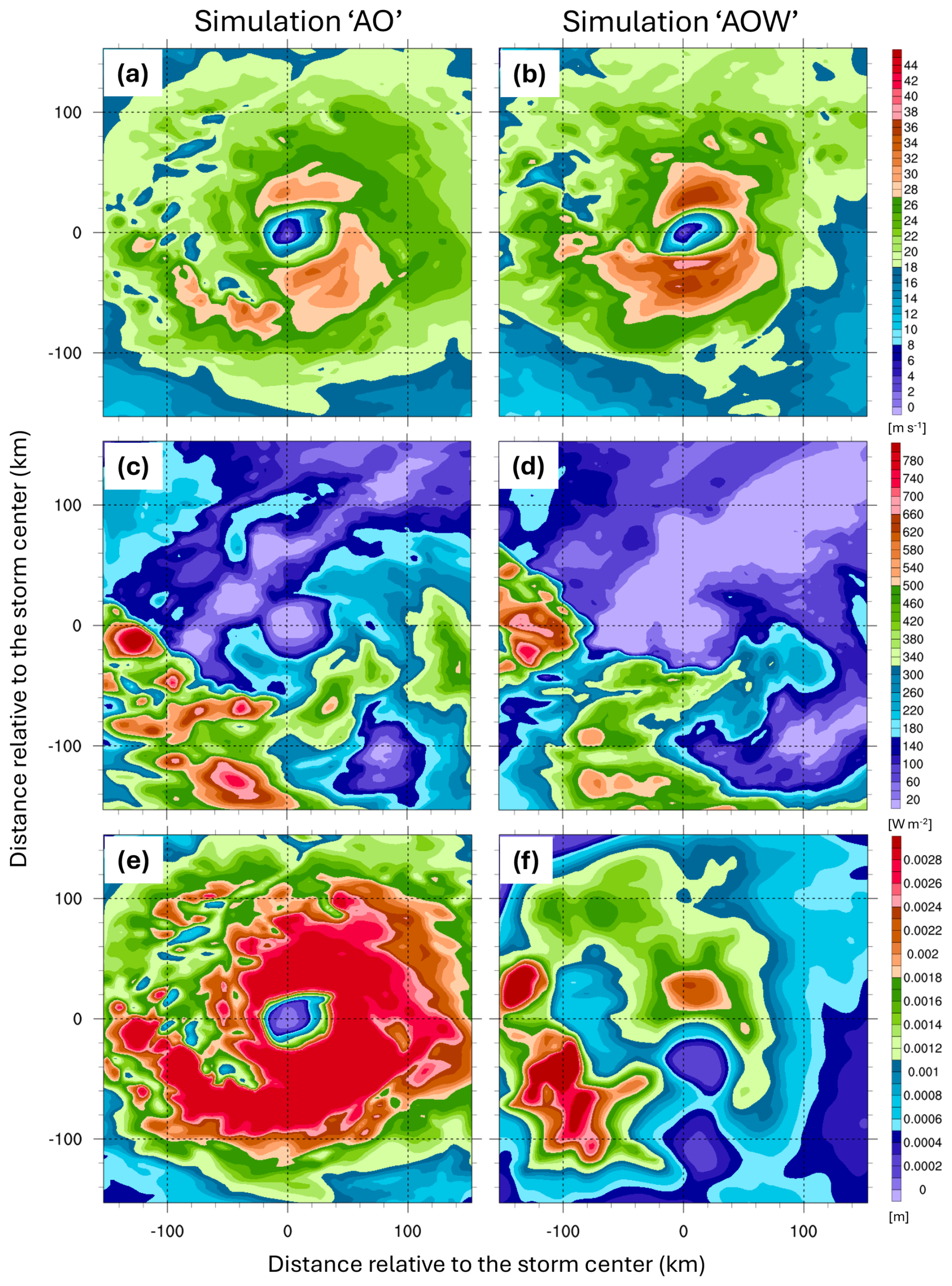
Figure 11 Distribution of (a–b) 10 m wind speed (m s⁻¹), (c–d) surface enthalpy flux (W m⁻²), and (e–f) surface roughness length (m) derived from experiment “AO” (left column) and experiment “AOW” (right column) at 12:00 UTC on 22 August 2021. All distributions are displayed in a 300 km × 300 km storm-centered coordinate.

An important question remains regarding the discrepancy between minimum SLP and maximum wind speed in “AO” and “AOW” simulations. Although “AO” produces a lower minimum SLP, it shows weaker maximum wind speeds than “AOW” – despite higher surface enthalpy and momentum fluxes at peak intensity (12:00 UTC, 22 August; Figs. 3b–c, 11a–b). As discussed, this is due in part to the higher Z₀ in “AO”, resulting from the absence of wave dynamics. Increased Z₀ leads to greater frictional drag, reducing near-surface wind speeds. This enhanced friction contributes to stronger subgradient winds, where actual wind speeds fall below those expected from gradient wind balance. The imbalance between forces in the boundary layer is described by the agradient force (AF), defined as

$$\begin{array}{}\text{(3)}& \text{Agradient Force (AF)}=-{\displaystyle \frac{\mathrm{1}}{\mathit{\rho }}}{\displaystyle \frac{\partial p}{\partial r}}+{\displaystyle \frac{V_{\mathrm{t}}^{\mathrm{2}}}{r}}+f{V}_{\mathrm{t}},\end{array}$$

where p is pressure, r is the radial distance from the TC center, V_t is the tangential wind speed, ρ is air density, and f is the Coriolis parameter. Near the surface, both “AO” and “AOW” deviate from gradient wind balance due to friction, which reduces V_t, weakening both the Coriolis and the centrifugal forces. With the pressure gradient force unchanged, this creates a negative agradient force (AF <0), driving radial inflow. This inflow forms part of the storm's secondary circulation. Its strength can indicate the degree of deviation from gradient wind balance – stronger inflow implies greater subgradient winds. Table 4 clearly shows that “AO” is associated with a stronger surface pressure gradient force, which, along with a higher Z₀, creates more favorable conditions for enhanced mass flux inflow. On the other hand, “AO” exhibits weaker absolute angular momentum (AAM), defined as

$$\begin{array}{}\text{(4)}& M=r{V}_{\mathrm{t}}+{\displaystyle \frac{\mathrm{1}}{\mathrm{2}}}f{r}^{\mathrm{2}}.\end{array}$$

As shown in Eq. (4), AAM is closely tied to the storm's rotational wind structure. Therefore, to better understand the discrepancy between “AO” and “AOW” – specifically why “AO” has a stronger pressure gradient but weaker winds – we analyze the AAM budget, following Zhang and Marks (2015) and Zhao et al. (2022). The AAM budget equation used is

$$\begin{array}{}\text{(5)}& \begin{array}{rl}{\displaystyle \frac{\partial \langle M\rangle }{\partial t}}& =-\langle V_{\mathrm{r}}\rangle {\displaystyle \frac{\partial \langle M\rangle }{\partial r}}-\langle w\rangle {\displaystyle \frac{\partial \langle M\rangle }{\partial z}}-\langle V_{\mathrm{r}}^{\prime }{\displaystyle \frac{\partial M^{\prime }}{\partial r}}\rangle \\ & -\langle w^{\prime }{\displaystyle \frac{\partial M^{\prime }}{\partial z}}\rangle +F_{\mathrm{r}},\end{array}\end{array}$$

where V_r and w denote the radial wind speed and vertical wind component, respectively. Brackets 〈〉 denote azimuthal averages, and primes indicate deviations from the mean. The left-hand side represents the time tendency of azimuthally averaged AAM. The right-hand side includes contributions from mean radial advection, mean vertical advection, radial eddy transport, vertical eddy transport, and the friction/residual term F_r. We hypothesize that the higher Z₀ in “AO” – a result of the simplified Charnock relation – enhances angular momentum dissipation and reduces wind speeds despite a stronger pressure gradient. Figure 12 presents the AAM tendency, mean radial advection, mean radial eddy transport, and F_r terms over the period from 00:00 to 12:00 UTC on 22 August 2021, during which both storms underwent steady intensification. The results indicate that the mean radial advection (Fig. 12b, f) and F_r (Fig. 12d, h) terms are particularly influential in determining the AAM tendency and tend to oppose each other. Within 100 km of the storm center, substantial AAM dissipation is observed in the F_r term for both simulations (Fig. 12d, h), aligning spatially with regions of elevated Z₀. However, this dissipation is much more pronounced in “AO” (Fig. 12d), suggesting that its higher Z₀ values may unrealistically amplify angular momentum loss, leading to weaker surface winds despite lower minimum SLP. These findings highlight the crucial role of air–sea interactions, particularly those induced by waves and related processes, in accurately simulating the wind structure of TCs within the marine boundary layer which impact offshore wind turbines.

Table 4 Spatially averaged metrics within 10–60 km of the storm center, vertically integrated through the boundary layer up to 1.2 km above the ground level, at 12:00 UTC on 22 August 2021. PGF indicates the pressure gradient force and is calculated at mean sea level.

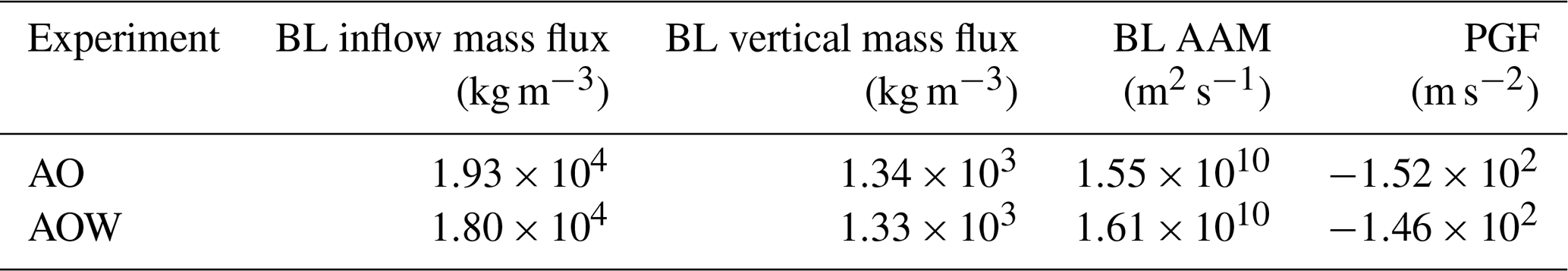
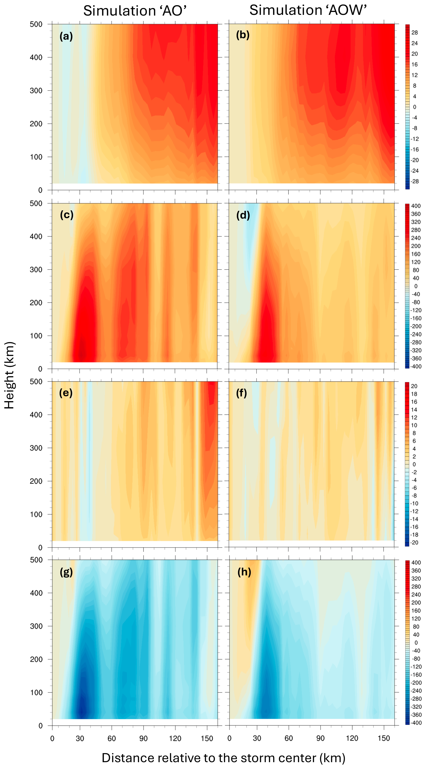
Figure 12 Radius–height plots of the terms in the azimuthally averaged absolute angular momentum budget: (a–b) time tendency term (m² s⁻²), (b) mean advection term (m² s⁻²), (c) eddy transport term (m² s⁻²), and (d) friction (m² s⁻²) and residual during the time from 00:00 to 12:00 UTC, 22 August 2021. The left column is derived from “AO” and the right column from “AOW”.

6 Summary and discussion

Previous studies of TC wind fields and their impacts on offshore wind turbines have primarily relied on atmosphere-only or empirical models, which neglect critical interactions among the atmosphere, ocean, and waves. This limitation hampers the accuracy of risk assessments for offshore wind infrastructure, particularly in hurricane-prone regions. This study developed a fully coupled modeling system (C-WFS) integrating WRF, FVCOM, and SWAN to simulate atmosphere–ocean–wave feedback on TC development and assess implications for offshore infrastructure. Using Hurricane Henri (2021) as a case study, chosen for its impact on the northeast US and available airborne observations, we ran three experiments of increasing complexity: “A”, “AO”, and “AOW”. These were evaluated against observations. All simulations overestimated intensity in terms of minimum SLP, but the fully coupled “AOW” reduced this bias during development and weakening stages. “AOW” also better captured 3D storm structure, especially low-level winds critical to coastal and offshore energy infrastructure. This improvement is attributed to wave-induced ocean mixing (cooling SST) and reduced surface roughness, resulting in more realistic wind fields and lower frictional loss of angular momentum. In contrast, “AO”, which lacks wave coupling, exhibited excessive surface roughness from a simplified parameterization dependent on wind only, causing greater frictional dissipation and weaker tangential winds despite a deeper central pressure. These results highlight the importance of including wave dynamics and incorporating dynamic and thermodynamic feedback among all three components for accurate TC intensity and structural forecasts.

The model also captures wind–wave misalignment and alignment, key processes often overlooked but crucial for evaluating structural loads, fatigue, and operational risks. Together, these enhancements yield a more realistic representation of storm evolution, intensity, and structure, underscoring the importance of fully coupled modeling systems for accurate risk assessments and the development of resilient offshore wind infrastructure.

While this study applied the C-WFS framework to Category 1 Hurricane Henri and highlighted the role of air–sea interactions in TC structure and intensity, it has not yet been applied to stronger storms or included sea spray effects, both of which are current limitations we are actively addressing. A key motivation behind this work is to better understand how coupled dynamics modulate TC wind fields across different intensities, particularly in regions with offshore wind farms, where storm structure and intensity can directly affect turbine loading, resilience, and operational risk.

Another open question is how the horizontal resolution of ocean components influences TC development in coupled models. While it is well established that finer atmospheric resolution improves storm intensity forecasts (e.g., Gentry and Lackmann, 2010; Prein et al., 2015), the effects of ocean resolution are less understood. Higher-resolution ocean grids can better resolve mesoscale and submesoscale features such as eddies and fronts, which influence SST patterns, air–sea fluxes, and upper-ocean mixing – factors critical to storm intensity and evolution (Zhang et al., 2023). These processes modulate SST cooling and ocean heat content redistribution during storm passage. Unlike traditional nested-grid approaches (e.g., in COAWST), C-WFS uses an unstructured mesh that smoothly transitions across resolutions, avoiding boundary artifacts. This flexibility makes C-WFS particularly well suited to explore how ocean resolution affects coupled dynamics and TC behavior – an area we aim to investigate in future work.

In parallel, this modeling framework presents a valuable opportunity to assess whether current IEC (2019a, b) standards for wind conditions, such as wind shear, veer, and turbulence, are adequate for regions prone to TCs. We are currently performing a comprehensive analysis using this fully coupled model to characterize the representation of these wind parameters, potentially informing revisions to design criteria that improve the structural resilience and reliability of offshore wind turbines under TC-induced loading conditions.