Continuous-lifetime-monitoring technique for structural components and main bearings in wind turbines based on measured strain and virtual load sensors

Decisions on the lifetime extension of wind turbines require evaluating the remaining useful life of major load-carrying components by making a comparison to the design lifetime. This work focuses on the lifetime assessment of two fundamentally different components: a structural component in the form of the tower and rotating components in the form of the main bearings. A method is presented that combines high-frequency SCADA, accelerometers, tower bottom and blade root strain gauge bridges, and limited design information for continued estimates of the component loads and their subsequent fatigue damage accumulations. The work is applied to a highly instrumented DTU research turbine, a Vestas V52 model, where strain gauges in the blade root and in the tower bottom are calibrated for nearly 10 years using continual calibration methods without the need for operator input. The lifetime estimates of the tower bottom and front and rear main bearings were found to be 2952, 282, and 566 years, respectively, reflecting the low average wind speed of the turbine site compared to the wind turbine design wind class IA. Secondly, it was investigated whether virtual load sensors can replace tower strain gauges. Consistent tower bottom strain signal estimates and long-term damage accumulation were achieved with ±5 % lifetime variability once SCADA, nacelle accelerometers, and blade root strain gauges were combined for the deployment of a long short-term memory (LSTM) neural network. A systematic underprediction of the accumulated damage of the tower bottom was observed for the virtual load sensors with a reduced set of inputs, and a correction method was proposed. Finally, the impact of environmental conditions, including turbulence intensity and shear exponent of the incoming wind, on the main bearing lifetime was investigated based on load measurements. A simple drivetrain thermal model was used to evaluate the modified lifetime L_10 m of the main bearings. Fatigue loads in the locating main bearing are driven by the peak of the turbine thrust curve, with higher loads observed at rated wind speed. An effect of longer main bearing lifetime with higher turbulence intensity was observed at rated wind speed and can be explained by the turbulence averaging of the thrust loads.

1 Introduction

The extension of the lifetime of wind turbines provides an opportunity to decrease the levelized cost of the electricity produced by wind turbines, which is not only competitive, but in many cases also the cheapest electricity source according to evaluations of multiple global benchmark reports (IEA and NEA, 2020; IRENA, 2024). At the same time, lifetime extension could decrease the global warming potential (CO₂ eq. kWh⁻¹) emitted during the entire life cycle of a wind turbine (UNECE, 2022).

Lifetime extension of wind turbines is often dictated by reliable technical evaluations of the consumed and the remaining useful lifetime of structural components such as the tower and the foundations (Ziegler et al., 2018; IEC-TS-61400-28, 2025). Such large components are site-specific, and little experience can be found in replacing them during and beyond the turbine lifetime, as this would hinder the profitability of a wind farm. Similarly, having unexpected and several load-carrying components failing would require long-lasting replacements that would increase the operational expenditure (OPEX) of a wind farm and reduce its revenue. That is the case with the main bearings. OPEX estimates should be based on the probability of failure of such components combined with their availability in the spare market.

As a main bearing replacement incurs significant costs and turbine downtime, this decision should be made with high levels of certainty. A main bearing failure results in high replacement costs, between USD 225 000 and 400 000, and loss of revenue due to production interruption, and its failure is one of the main reasons for the increase in OPEX, especially in onshore wind turbines of 2 to 6 MW in size according to Pulikollu et al. (2024). Although main bearings are known to have multiple failure modes, as examined by Hart et al. (2020), including abrasive and adhesive wear and fretting, this work considers lifetime consumption as the fatigue life consumption of the main bearing. This is due to the leading role of rolling contact fatigue (RCF), which cannot yet be ruled out with respect to historical replacement data of the main bearings. Hart et al. (2023) carried out a large review of historical data on the damage and failure of the main bearing and identified that for a large share (80 %) of the reported failures, spalling was present, which could be a consequence of both subsurface- and surface-initiated RCF.

In this context, the end goal of a well-designed structural health monitoring (SHM) campaign is to have the most comprehensive and reliable wind turbine monitoring and lifetime estimation with the least amount of instrumentation (d N Santos et al., 2022). And using strain gauges often results in one key drawback: compromised long-term reliability. There has been a literature gap on the possibility of calibrating strain gauges for many years, with only some investigations to note (Pacheco et al., 2024). Therefore, the question of how to extrapolate the lifetime of components based on limited recordings has been of interest and widely investigated (Loraux and Brühwiler, 2016; Hübler and Rolfes, 2022; Sadeghi et al., 2024; de N Santos et al., 2024). However, no consensus has yet been reached on the methods or uncertainties related to those methods. In this context, data-driven methods (Dimitrov and Göçmen, 2022; Pimenta et al., 2024) deployed as long-term virtual load sensors could yield several advantages by replacing real sensors and reducing the amount of instrumentation needed and being able to describe complex mathematical correlations, with no real physical understanding of the system.

Considering the challenges and gaps identified, this work aims to use existing onboard sensors and limited non-invasive hardware additions to evaluate the lifetime of structural and rotating components simultaneously. The following research questions guided the methodology and subsequent analysis.

• Is it possible to continuously and reliably count the lifetime of a tower and a four-point configuration main bearing without blade design information and having access to SCADA, blade root strain gauges, and tower bottom strain gauges while meeting ISO-281 (2007) and IEC 61400-1 (2019) standards?

• What degree of accuracy could be achieved by a tower bottom virtual load sensor based on measurements in the nacelle?

• What are the environmental and operation conditions (EOCs) which have the strongest impact on the basic and modified rating lifetime of the main bearing (L₁₀ and L_10 m, respectively), based on analysis of a long-term-measured dataset?

The remaining sections of this paper are organized as follows. Section 2 provides an overview of the theoretical background relevant to this work, including the assumptions behind the tower fatigue lifetime and the main bearing lifetime, as well as the concept of virtual load sensors applied in this study. Section 3 describes the wind turbine and the environmental measurement campaign used for data collection. Section 4 details the proposed methodology for the calibration of the strain gauge and the lifetime of the tower and main bearing based on load measurements and virtual load sensors. The results obtained are presented in Sect. 5, including a discussion of the findings compared to the relevant literature, and key correlations are analyzed. Section 6 concludes the paper by summarizing the main insights and learning takeaways from this work.

2 Theoretical background

The concept of tower fatigue and main bearing lifetime is assumed to be derived from standards used for design and certification. The concept of virtual load sensors can also be very broad. In this work, we focus on time series and data-driven virtual load sensors that could be used to replace tower bottom strain gauges in the case of sensor failure. More details on each subject are described in the following subsections, with Fig. 2 providing an overview of the methodology.

2.1 Tower fatigue lifetime

The lifetime is estimated as described by IEC 61400-1 (2019), considering design load cases (DLCs) 1.2 (power production), 3.1 (start-up), and 4.1 (normal shutdown). More details on how to classify these operational conditions based on 10 min SCADA can be found in Faria et al. (2024). On the material side, the tower of the DTU research V52 turbine is made of structural steel S355, which is often used in large components and harsh environmental conditions. In this work, the fatigue assessment of critical welds assumes that the component has inherent defects in the welded joints and thus does not model crack initiation or growth.

The first step is to convert a measured tower bending strain ϵ [µmm mm⁻¹] to bending stress σ [Pa] as shown by Hooke's rule $\mathit{\sigma }=E\cdot \mathit{ϵ}$. The bending stress can be translated into the bending moment M assuming the tower is an Euler–Bernoulli beam:

$$\begin{array}{}\text{(1)}& \mathit{\sigma }={\displaystyle \frac{M\cdot c}{I}},\end{array}$$

where I [m⁴] is the area moment of inertia, and c [m] is the radius, in the case of a circular cross section. To evaluate fatigue, the stress time series is converted to stress ranges Δσ_i and number of cycles n_i using the rainflow counting technique, as described by ASTM E1049-85 (2017). The tower bottom in this work is evaluated using the “D” category of the stress cycle (SN) curve for butt welding in air, as suggested by DNVGL-RP-C203 (2016), which translates Δσ_i into a maximum number of cycles to failure N_max,i. Finally, fatigue accumulation – in other words, fatigue lifetime – is assumed to be linear, according to Palmgren and Miner (1945), which is valid for any time window, from high-frequency to 10 min instances to lifetime.

$$\begin{array}{}\text{(2)}& D_{\mathrm{T}}=\sum _j^{N_j}{D}_{\mathrm{T},j}=\sum _j^{N_j}\sum _i^{Ni}{\displaystyle \frac{n_i}{N_{\max ,i}}}=\sum _j^{N_j}\sum _i^{N_i}{\displaystyle \frac{n_i\cdot (\mathrm{\Delta }{\mathit{\sigma }}_i{)}^{m_i}}{K_i}}\end{array}$$

Here D_T is the tower accumulated fatigue damage (failure at unity), D_T,j is the accumulated fatigue damage of the 10 min instance, m_i is the exponent of the SN curve, K_i is the intercept of the SN curve on the y axis, N_j is the number of 10 min instances, and N_i is the number of cycles in a given instance.

The non-linear nature of fatigue can be observed from the SN curve having different m_i and K_i dependent on the two regions of the SN curve where the cycle could be placed. In order to facilitate the evaluation of the virtual load sensor during training and validation, instead of comparing D_T, damage equivalent loads (DELs) are often used and can be explained as single-frequency sinusoidal loads that would inflict the same damage as the initial load variable in time, as in

$$\begin{array}{}\text{(3)}& \text{DEL}={\left(\sum _i^{N_i}{\displaystyle \frac{n_i\cdot \mathrm{\Delta }{\mathit{\sigma }}_i^m}{N_{\mathrm{ref}}}}\right)}^{\mathrm{1}/m},\end{array}$$

where m is assumed to be 4, which is an average between DNV “D” curve values of m_i equal to 3 and 5 and ${\log }_{K_i}$ equal to 12.164 and 15.606, respectively, transitioning at N_max equal to 10⁷ cycles. N_ref is a normalization factor and is arbitrarily assumed to be 10⁷ cycles, since DEL has no absolute meaning.

For the estimation of the consumed and remaining useful lifetime of a tower, and the deployment of the virtual load sensor over long periods, DEL has no absolute meaning, and its uncertainty underestimates the uncertainty of the useful life of the component, and, therefore, D_T should be prioritized. More discussion is present in Sect. 5.3.

2.2 Main bearing fatigue lifetime

The lifetime of a rotating component, such as a main bearing, can be significantly more complex to model than the tower lifetime. In this work, the formulations from ISO-281 (2007) are followed, which also define the linear accumulation of damage as proposed by Palmgren, using the same DLCs as for the tower. As mentioned, rolling contact fatigue is not the only damage mode of the main bearings, but the inclusion of additional mechanisms is not in the scope of the present work.

The radial F_r [N] and axial F_a [N] load acting on the main bearings are combined into

$$\begin{array}{}\text{(4)}& P=X\cdot F_{\mathrm{r}}+Y\cdot F_{\mathrm{a}},\end{array}$$

where P [N] is the dynamic load, and X and Y are functions of the load ratio $F_{\mathrm{a}}/F_{\mathrm{r}}$ and the limiting value e, as often provided by the bearing manufacturer. The time-varying P can be replaced by a constant equivalent load P_eq that would have the same deterioration at its given operational rotation speed, similar to the defined DEL, without involving any counting method.

$$\begin{array}{}\text{(5)}& P_{\mathrm{eq}}={\left({\displaystyle \frac{\sum P_i^p\cdot {\mathit{\omega }}_i}{\sum {\mathit{\omega }}_i}}\right)}^{\mathrm{1}/p}\end{array}$$

Here P_i [N] is the dynamic load; p is the exponent dictated by the type of rolling body (e.g., ball or roller), as provided by ISO-281 (2007); and ω_i [rpm] is the rotational speed of the main bearing at the instantaneous i timestamp.

Then, the basic rating life L₁₀ is defined as the 90 % survival time of a given population of main bearings under similar operational conditions. In other words, 10 % of the bearings would fail.

$$\begin{array}{}\text{(6)}& \begin{array}{rl}{L}_{\mathrm{10},j}& ={\mathrm{10}}^{\mathrm{6}}{\left({\displaystyle \frac{C_{\mathrm{d}}}{P_{\mathrm{eq}}}}\right)}^p\left[\text{revolutions}\right]\\ L_{\mathrm{10},j}& ={\displaystyle \frac{{\mathrm{10}}^{\mathrm{6}}}{\mathrm{60}\cdot \mathit{\omega }\cdot \mathrm{8760}}}{\left({\displaystyle \frac{C_{\mathrm{d}}}{P_{\mathrm{eq}}}}\right)}^p\left[\text{years}\right]\\ L_{\mathrm{10}}& ={\displaystyle \frac{\mathrm{1}}{\sum {\mathit{\varphi }}_j/L_{\mathrm{10},j}}}\left[\text{years}\right]\end{array}\end{array}$$

Here L₁₀ is the basic rating life overall, while L_10,j is the basic rating in a given 10 min instance j. If all instances have the same 10 min, ϕ_j is the inverse of the number of instances. C_d [N] is the dynamic load rating, P_eq [N] is the equivalent dynamic load, and ω [rpm] is the rotational speed of the main bearing within a 10 min instance. Once L₁₀ is calculated as the number of hours to failure in each instance, one can describe a main bearing damage accumulation, similar to the damage accumulation in the tower, as in

$$\begin{array}{}\text{(7)}& D_{\mathrm{B}}=\sum _j^{N_j}{D}_{\mathrm{B},j}={\displaystyle \frac{t_{\mathrm{operation}}}{L_{\mathrm{10}}}},\end{array}$$

where D_B is the accumulated fatigue damage of the main bearing (failure at unity), D_B,j is the accumulated fatigue damage of the 10 min instance, and t_operation is the evaluated time of operation in years.

To account for operating conditions more realistically, the life modification factor a_ISO (ISO-281, 2007) is evaluated for the main bearing. This factor accounts for variations in operating temperature and lubricant condition and is influenced by grease cleanliness, operating viscosity (temperature dependent), rolling element type, bearing fatigue limit, and external loads (Needelman and Zaretsky, 2014). The modified rating life L_10 m of the main bearing is then calculated using

$$\begin{array}{}\text{(8)}& L_{\mathrm{10}\mathrm{m},j}=L_{\mathrm{10},j}\cdot a_{\mathrm{ISO},j},\end{array}$$

where a_ISO,j is the modification factor calculated for each 10 min instance j. In this work, a drivetrain thermal model is used to allow the estimation of a_ISO,j, as shown in Sect. 4.2.1. L_10 m,j can be accumulated as given in Eq. (6) for L₁₀.

2.3 Virtual load sensors

In this work, virtual load sensors are seen as an opportunity to replace physical sensors to estimate tower bottom bending moments and long-term fatigue lifetime. In the literature, several efforts have been made with regard to data-driven (machine learning) models for lifetime predictions of components.

Benefiting from 10 min instance statistics (e.g., mean and standard deviation) and more available SCADA accelerometers, efforts have been made to estimate target statistics such as damage equivalent loads (DELs) or damage to the main bearing. Mehlan et al. (2023) estimated aerodynamic hub loads and tracked bearing fatigue damage using a digital-twin-based virtual sensing combining SCADA and condition monitoring. For support structures, de N Santos et al. (2024) estimated the fatigue lifetime based on different combinations of SCADA levels, highlighting the improvement in performance using reliable nacelle accelerometers, with a novel population-based approach for wind farm extrapolation. Focusing on time extrapolation, Hübler and Rolfes (2022) focused on different methodologies to extrapolate damage in time and their estimated uncertainty. On the other hand, when the time series signal is the target output, the model selection and training process are quite different. Complementarily, Dimitrov and Göçmen (2022) showed how machine learning time series models (e.g., long short-term memory, LSTM) can act as virtual sensors for blade root bending moments trained on aeroelastic simulations. Gräfe et al. (2024) trained neural networks on simulated floater motions and lidar-derived wind to estimate the tension and DEL of mooring lines.

The same data-driven models applied by Dimitrov and Göçmen (2022) are selected to be used in this work on the DTU research V52 turbine dataset, all derivatives of neural network architectures. This work's contribution to virtual load sensor methods lies in the validation of a model that should accurately replicate both (1) the time series of tower bottom bending moments and (2) the fatigue loads of the tower and main bearings in the long term. (1) The first can have its performance quantified by using the virtual load sensor as a thrust estimate to calculate the lifetime consumption of the main bearings. (2) The latter includes the three most damaging operational conditions for the tower as described in Pacheco et al. (2024) and Faria et al. (2024): power production (DLC 1.2), start-up (DLC 3.1), and shutdown (DLC 4.1), all in a single model.

3 Measurements

In this work, SCADA data and measurements over nearly 10 years are analyzed from 2016 to 2024 (inclusive) in Risø, Denmark. The environmental conditions are analyzed out of 10 min instance statistics from a met mast about 100 m east of the DTU research V52 turbine. In addition to the mean wind speed U_hub at the hub height of z_hub=44 m, the turbulence intensity is calculated as $\text{TI}={\mathit{\sigma }}_U/U$, where σ_U is the standard deviation of the wind speed. Moreover, vertical shear is modeled considering the normal wind profile model (IEC 61400-1, 2019) given by the power law equation $U\left(z\right)=U_{\mathrm{hub}}(z/z_{\mathrm{hub}}{)}^{\mathit{\alpha }}$, where z is the height, and α is the shear exponent. The latter is estimated as the best-fitting factor out of five different cup anemometers measuring heights (at 18, 31, 44, 57, and 70 m) for each 10 min instance. No shadow correction was performed for the mast tower. In general, it is possible to observe that the Risø site has fairly low-wind and constant-wind-flow conditions over the years. The yearly wind speed U_hub has a mean value of 5.6 m s⁻¹. The site reference turbulence I_ref, calculated as $I_{\mathrm{ref}}={\mathit{\sigma }}_U/(\mathrm{0.75}{U}_{\mathrm{hub}}+\mathrm{5.6})$, has a mean value around 0.08 (closer to IEC class C) and the shear exponent α around 0.22. The prevailing wind direction falls within the southwest quadrant across all years. The DTU research V52 turbine is a Vestas 850 kW onshore wind turbine class IA with a rotor diameter of 52 m and a hub height of 44 m, with a active pitch and rotor speed control. SCADA and SHM measurements are available from February 2016 to December 2024, as are statistics and high-frequency data. The turbine has a rated wind speed of approximately 14 m s⁻¹. Figure 1 represents the turbine schematic and part of its instrumentation, highlighting the two measurement setups present in the tower bottom (a–a) and blade root (b–b). SCADA includes rotor speed ω, pitch angle θ, yaw angle γ, azimuth angle φ, and power. All of the bending moments shown are obtained from full Wheatstone bridges installed in the components. This configuration has a couple of important advantages as it has a higher signal-to-noise ratio, is temperature independent, and is optimized for measuring bending stress (Hoffmann, 1989). A problem in the quality of the azimuth angle φ measured by a proximity sensor on the shaft flange was identified before 2018 and after 2022, probably due to surface dirt. A correction was applied to all the raw signal to account for that, by combining the controller rotor speed signal with the measured azimuth to have a more reliable estimate of the azimuth angle (refer to Appendix A). Taking into account Fig. 1c₁, the tower bottom fore–aft bending moment M_fore−aft (downwind) can be calculated as in Eq. (9).

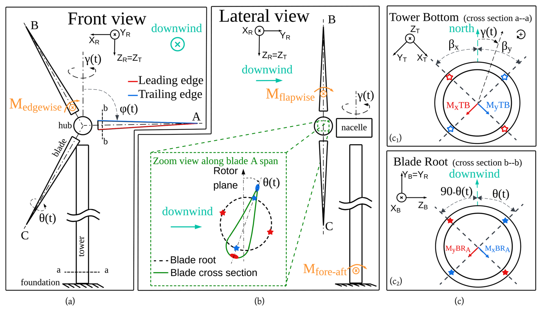
Figure 1 Schematic of an onshore wind turbine used to represent the DTU research V52 turbine parameters and measurements. (a) Front view shows the rotor coordinate system XYZ_R, which rotates with the yaw angle γ(t) around Z_T and faces the wind direction. The azimuth angle φ(t) of blade A and pitch angle θ(t) are also shown. M_edgewise represents the edgewise (in-plane) blade root bending moment. (b) In the lateral view, the flapwise (out-of-plane) rotor bending moment M_flapwise and the tower bottom fore–aft bending moment M_fore−aft are shown. The θ(t) angle is the controller-defined blade root angle between the rotor plane and the chord line of the blade, as shown in the zoomed-in view (dashed green box). (c₁) Tower bottom cross section (a–a) in the global/tower coordinate system (time-invariant) XYZ_T is determined. M_fore−aft is dependent on γ(t), as a composition of the measured tower bottom bending moments MxTB and MyTB, which are obtained from strain gauges (stars) installed at the angles −β_x and β_y, respectively. (c₂) Blade root A cross section (same setup for blades B and C) shown in the blade coordinate system XYZ_B, which rotates with φ(t) with respect to Y_R. Both measured blade root bending moments M_xBR_A and M_yBR_A will be converted into M_flapwise and M_edgewise as a function of the pitch angle θ(t).

$$\begin{array}{}\text{(9)}& M_{\mathrm{fore}-\mathrm{aft}}\left(t\right)={\displaystyle \frac{\left(-M_{x}TB\left(t\right)\cdot \sin \left({\mathit{\beta }}_y-\mathit{\gamma }\left(t\right)\right)+M_{y}TB\left(t\right)\cdot \sin \left({\mathit{\beta }}_x+\mathit{\gamma }\left(t\right)\right)\right)}{\sin \left({\mathit{\beta }}_x+{\mathit{\beta }}_y\right)}}\end{array}$$

Here the denominator factor is imposed because the two tower bottom bending moments are not perpendicular. Similarly, considering the measurement setup shown in Fig. 1c₂, the blade root flapwise M_flapwise (out-of-plane) and edgewise M_edgewise (in-plane) bending moments can be calculated individually for blades A, B, and C.

$$\begin{array}{}\text{(10)}& {\displaystyle }\begin{array}{rl}{M}_{\mathrm{flapwise},(\mathrm{A},\mathrm{B},\mathrm{C})}\left(t\right)& =M_{x}B{R}_{(\mathrm{A},\mathrm{B},\mathrm{C})}\left(t\right)\cdot \cos \left(\mathit{\theta }\left(t\right)\right)\\ & -M_{y}B{R}_{(\mathrm{A},\mathrm{B},\mathrm{C})}\left(t\right)\cdot \sin \left(\mathit{\theta }\left(t\right)\right)\end{array}\text{(11)}& {\displaystyle }\begin{array}{rl}{M}_{\mathrm{edgewise},(\mathrm{A},\mathrm{B},\mathrm{C})}\left(t\right)& =M_{x}B{R}_{(\mathrm{A},\mathrm{B},\mathrm{C})}\left(t\right)\cdot \sin \left(\mathit{\theta }\left(t\right)\right)\\ & +M_{y}B{R}_{(\mathrm{A},\mathrm{B},\mathrm{C})}\left(t\right)\cdot \cos \left(\mathit{\theta }\left(t\right)\right)\end{array}\end{array}$$

4 Methodology

Figure 2 shows the inputs and assumptions taken into account to investigate the research questions, from high-frequency turbine measurements to tower (structural component) D_T and main bearing (rotating component) D_B accumulation of fatigue damage over time. The orange boxes include the continual calibration of the strain gauges and the operations to translate the strain measurements of the tower and the blade into the tower bottom bending moment M_fore−aft and the axial F_a and radial F_r main bearing loads. The standards shown (DNVGL-RP-C203, 2016; IEC 61400-1, 2019; ISO-281, 2007) provide the methods for the fatigue lifetime evaluations of each component, as explained in Sect. 2. The DTU research V52 turbine has an S355 steel tower, with a measured tower geometry consisting of a 2.913 m outer diameter and 16 mm wall thickness.

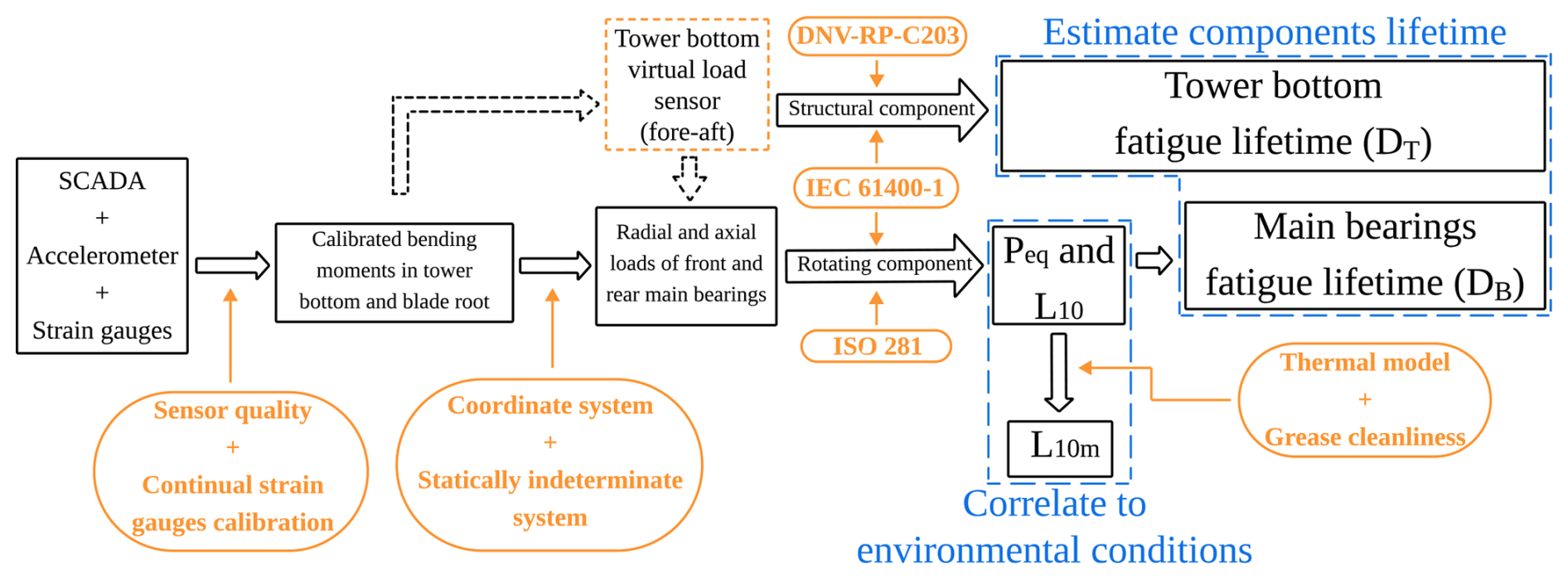
Figure 2 Methodology flowchart presenting the steps followed in this work, starting from high-frequency measurement and the SCADA dataset to component lifetime estimates. The rectangular black boxes refer to measurement signals and estimates. Tower bottom D_T and main bearing D_B fatigue lifetimes are analyzed over time, and the equivalent dynamic load P_eq, basic rating life L₁₀, and modified rating life of the main bearing L_10 m are analyzed as a function of environmental conditions. The orange boxes identify the procedures and standards used in this work. The dashed orange box contains the tower bottom virtual load sensor, which should replace the real sensor in the case of sensor failure.

In addition, a virtual load sensor is proposed to replace real strain gauges in the event of sensor failure, and its performance is assessed for fatigue lifetime estimations. The main bearing equivalent dynamic load P_eq, the basic L₁₀ rating life, and the modified L_10 m rating life are evaluated as a function of key environmental conditions. To compute L_10 m of the main bearings, a drivetrain thermal model was made to estimate the temperature of the main bearings, which is necessary to estimate the life modification factor a_ISO, as introduced in Sect. 2.2.

4.1 Strain gauge zero-drift automatic calibration

It is often claimed that strain gauges are only reliable for short-term (less than a year) to mid-term (couple of years) campaigns, a limitation that would conflict with the requirement for sustained monitoring of wind turbine structural elements, most notably in offshore installations, where replacement in the case of sensor failure is expensive and can take time due to weather windows.

This work overcomes such a limitation by introducing continual and automated routines for the calibration of both tower bottom and blade root strain gauges that work on long-term datasets (almost a decade). The methods do not require operator intervention, stopping, or curtailment and instead take advantage of idling and parked conditions. Both methodologies are derived from the recommendations in IEC 61400-13 (2016). The main objective is to identify the artificial offset O from the measured strain gauges and to correct them to the original zero point. The signals of the tower bottom and blade root bending moments, shown in Fig. 1, should be understood as $M=G\cdot (M_{\mathrm{raw}}+O)$, where M is the corrected bending moment, M_raw is the measured voltage signal, G is the gain associated with the translation of voltage readings into the bending moment, and O is the artificial offset of the strain sensor. It should be noted that for the tower bottom strain gauges placed on steel, G can be analytically calculated, depending on the bridge arrangement (full Wheatstone bridge in the DTU research V52 turbine), the elastic modulus, and the geometry. However, for blade root strain gauges mounted on composite material, a blade pull exercise must be performed to estimate G. Additionally, a crosstalk correction has to be applied considering the geometry of the twisted and nonsymmetric blade; see Papadopoulos et al. (2000). Such a calibration campaign has been undertaken on the DTU research V52 turbine, but detailed results are not presented in this work for confidentiality reasons.

4.1.1 Yaw sweeps and low-speed idling (LSI)

The tower bottom strain gauge calibration is based on a specific operation in which the wind turbine is parked and untwists its power cable at low wind speed. In that case, the turbine performs full yaw rotations, and the main contribution to the tower bottom bending moment is the gravitational load from the nacelle mass overhang bending moment. If at least 1 min data points of the yaw angle γ are available, the high-frequency strain gauge signals M_xTB and M_yTB can be automatically calibrated (Faria et al., 2024). The Python package generated for this matter is publicly available in Faria and Jafaripour (2023). The blade root strain gauge calibration is performed based on both idling and parked conditions at low wind speed. The first is used to calibrate the strain gauges placed on the pressure–suction surfaces of the blade. The latter is for those on the leading–trailing edges. The azimuth angle φ is needed at a higher sampling frequency (e.g., tested with at least 1 Hz). More information on the implementation can be found in Pacheco et al. (2024) and Faria et al. (2025).

4.2 Main bearing loads and temperatures

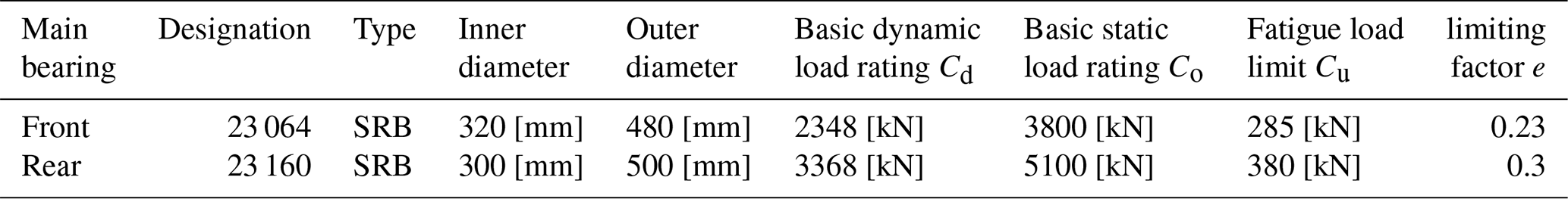
The front and rear main bearings of the DTU research V52 turbine are described in Table 1. The drivetrain transmits the torque from the rotor to the gearbox through the main shaft, which is supported by two spherical roller bearings in the main bearing housing and the gearbox upfront bearing, as shown in Fig. 3a.

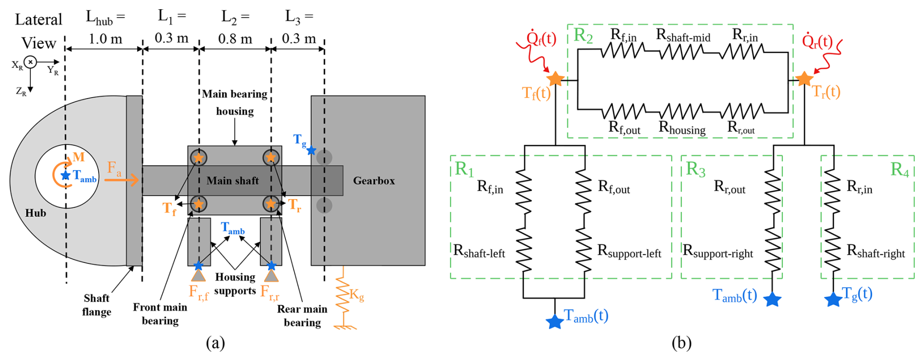
Figure 3 (a) Schematic of the DTU research V52 drivetrain and main bearing estimated front T_f and rear T_r temperatures. The hub carries the blades and their aerodynamic bending moment M and axial load F_a. The hub is bolted to the shaft flange. The shaft is supported by two main bearings, which are mounted inside the main bearing housing. The latter is clamped to the nacelle bed plate through the housing supports, equivalent to the front F_r,f and rear F_r,r main bearing radial load F_r. The gearbox is mounted by the torque arms but in a non-rigidly stiff connection point with stiffness K_g. (b) Simplified thermal circuit model of the drivetrain, which assumes that each 10 min instance reaches thermal equilibrium. Ambient temperature T_amb is measured in the nearby met mast, and the gearbox temperature T_g is estimated based on a 6-month monitoring record of the temperature of the gearbox wall facing the rear main bearing. ${\dot{Q}}_{\mathrm{r}}$ and ${\dot{Q}}_{\mathrm{f}}$ are the power dissipated by the main bearings. R represents the equivalent thermal resistance: R₁ between the front main bearing and ambient temperature, R₂ between the main bearings, R₃ between the rear main bearing and the ambient temperature, and R₄ between the rear main bearing and the gearbox close to the surface of the rear main bearing. Other heat exchanges are not considered. R_(…) values are estimates of the geometry of the drivetrain components (assumed to be steel) and bearing heat transfer coefficients, suggested by Schaeffler TPI-176 (2014).

The main bearing housing is clamped to the nacelle bed plate, while the gearbox is mounted through its torque arms in a rubber support. The rubber support is assumed to have a linear and temperature-independent spring with a stiffness of 20×10⁶ [N m⁻¹], close to the values suggested in Haastrup et al. (2011) and Keller et al. (2016). In Sect. 5.5.1, a sensitivity analysis is performed to evaluate the importance of this assumption.

Table 1 Technical specification of the two main bearings in the DTU research V52 turbine given by SKF Group (2025). SRB stands for spherical roller bearing and the bearing exponent $p=\mathrm{10}/\mathrm{3}$.

The aerodynamic bending moment M driven by the blades in the vertical M_v and horizontal M_h directions can be estimated from the blade out-of-plane bending moments using

$$\begin{array}{}\text{(12)}& {\displaystyle }\begin{array}{rl}{M}_{\mathrm{v}}\left(t\right)& =M_{\mathrm{flapwise},\mathrm{A}}\left(t\right)\cdot \cos \left(\mathit{\phi }\left(t\right)\right)+M_{\mathrm{flapwise},\mathrm{C}}\left(t\right)\\ & \cdot \cos \left(\mathit{\phi }\left(t\right)+\mathrm{120}\right)+M_{\mathrm{flapwise},\mathrm{B}}\left(t\right)\cdot \cos \left(\mathit{\phi }\left(t\right)+\mathrm{240}\right),\end{array}\text{(13)}& {\displaystyle }\begin{array}{rl}{M}_{\mathrm{h}}\left(t\right)& =M_{\mathrm{flapwise},\mathrm{A}}\left(t\right)\cdot \sin \left(\mathit{\phi }\left(t\right)\right)+M_{\mathrm{flapwise},\mathrm{C}}\left(t\right)\\ & \cdot \sin \left(\mathit{\phi }\left(t\right)+\mathrm{120}\right)+M_{\mathrm{flapwise},\mathrm{B}}\left(t\right)\cdot \sin \left(\mathit{\phi }\left(t\right)+\mathrm{240}\right),\end{array}\end{array}$$

where φ(t) is the azimuth angle of blade A; see Fig. 1. It should be noted that a positive M_v should benefit the loads in the radial main bearings to some extent, as it counter-balances F_rotor.

The main shaft is supported in four points, two main bearings, and the gearbox mounts, and it is solved as a statically indeterminate system. The radial clearance from the bearings is not explicitly considered. To solve the system of equations, the shaft is modeled as a flexible beam, and a double integration method is applied to compute the radial load of the front F_r,f and rear F_r,r main bearings (see Appendix B). Both aerodynamic and gravitational loads are included to estimate the radial loads. The resultant radial loads of the front F_r,f and rear F_r,r main bearings have a magnitude of

$$\begin{array}{}\text{(14)}& F_{\mathrm{r},(\mathrm{f},\mathrm{r})}=\sqrt{F_{\mathrm{r},(\mathrm{f},\mathrm{r}),\mathrm{v}}^{\mathrm{2}}+F_{\mathrm{r},(\mathrm{f},\mathrm{r}),\mathrm{h}}^{\mathrm{2}}},\end{array}$$

where “v” represents the vertical direction and “h” the horizontal direction (no static gravitational loads), as shown in Appendix B, and are solved individually for each main bearing.

The axial load F_a of the main bearings is equal to the thrust estimate, derived as the bending moment M_fore−aft divided by the height difference between the hub height and the tower bottom strain gauge. This is an assumption of this methodology, where the thrust estimate is linearly related to the bending moment of the bottom of the tower. Since both bearings can carry axial loads, the system may become over-constrained, causing additional axial stress during thermal expansion. For these reasons, the rear bearing is considered the locating bearing, being the bearing with smaller axial internal clearance.

Drivetrain thermal model

In the case that the temperature measurements of the main bearings are not available, estimates of the temperature of the main bearings are necessary to incorporate the life modification factor a_ISO. The a_ISO factor is a function of viscosity, which is a function of the lubricant temperature. Figure 3a shows the estimated temperatures from the rear T_r and front bearing T_f, together with the measured temperatures, ambient T_amb, and gearbox wall T_g. It is proposed to simplify the heat exchange between the heat dissipated by the bearings and the outer system (drivetrain), assuming thermal equilibrium in each 10 min instance and thermal resistors, as shown in Fig. 3b. The ambient temperature T_amb is measured using a spinner anemometer at the hub, and the gearbox temperature T_g is estimated based on 6-month monitoring campaigns that recorded the temperature of the gearbox wall facing the rear main bearing. A SCADA-based feed-forward neural network (FNN) model was trained to estimate the values of T_g for each 10 min instance.

$$\begin{array}{}\text{(15)}& {\displaystyle }{\dot{Q}}_{\mathrm{f}}-{\displaystyle \frac{(T_{\mathrm{f}}-T_{\mathrm{amb}})}{R_{\mathrm{1}}}}-{\displaystyle \frac{(T_{\mathrm{f}}-T_{\mathrm{r}})}{R_{\mathrm{2}}}}=\mathrm{0}\text{(16)}& {\displaystyle }{\dot{Q}}_{\mathrm{r}}+{\displaystyle \frac{(T_{\mathrm{f}}-T_{\mathrm{r}})}{R_{\mathrm{2}}}}-{\displaystyle \frac{(T_{\mathrm{r}}-T_{\mathrm{amb}})}{R_{\mathrm{3}}}}+{\displaystyle \frac{(T_g-T_{\mathrm{r}})}{R_{\mathrm{4}}}}=\mathrm{0}\end{array}$$

By applying the Kirchhoff circuit concept for thermal equilibrium, Eqs. (15) and (16) are obtained, which have two target variables, T_f and T_r, and the thermal resistances, R_i, defined in Fig. 3b. The dissipated power of a bearing is also affected by the bearing temperature (e.g., ${\dot{Q}}_{\mathrm{f}}=f(T_{\mathrm{f}},\mathrm{\dots })$), as the latter influences the viscosity of the lubricant (the base oil of the grease according to ASTM D341-93, 1998). Because the variables depend on one another, the equations are coupled and cannot be solved explicitly. Instead, a Newton–Raphson solver was implemented to iteratively estimate the results. This framework can be found in more detail in HIPERWIND D5.1 (2023). The dissipated powers were modeled as suggested by Schaeffler TPI-176 (2014), which separates them into two contributions: frictional heat driven by speed and frictional heat driven by load. The grease has been assumed to be Klüberplex BEM 41-301, a widely distributed industrial grease for wind turbine main bearings. Once T_r and T_f are estimated, a_ISO can be calculated as a function of the viscosity ratio κ, the assumed grease cleanliness level (see Sect. 5.5.3), C_u, and P_eq, as given by ISO-281 (2007).

4.3 Tower bottom virtual load sensor: thrust and fatigue loads

The selection of good candidates for the machine learning model to be deployed as virtual load sensors was carried out from simpler to more complex neural network architectures. Pure spatial correlation between the target variable and inputs is tested using an FNN baseline model (Rumelhart et al., 1986). Temporal correlation is added through an FNN with n-lagged time steps, the so-called NlaggedFNN (Dimitrov and Göçmen, 2022), and a long short-term memory (LSTM) neural network (Bengio et al., 1994). The first can only take a few time steps to still be “trainable”, while LSTM is often a less noise-sensitive model and can better capture long-term dependencies (Bengio et al., 1994) at the cost of model complexity. The hyperparameters of the models were tuned using the Keras-tuner random search method (O'Malley et al., 2019) using 10 h of data and three seeds per iteration. The bounds and the optimal hyperparameters for the models are included in Appendix C. All models used the “relu” activation curve in the hidden layers and “linear” activation towards the output layer. The LSTM model had a fixed “LSTM” layer and a second hidden layer with the same number of neurons (hidden units) as the first layer. The size of the training dataset was 160 h of data selected using a K-means clustering technique (Pedregosa et al., 2011), spreading the training space within the rotor speed, blade pitch, power, and DLCs to cover the relevant operational conditions. Similarly to Dimitrov and Göçmen (2022), training dataset size and sampling frequency sensitivity tests were carried out to use optimum values. In addition, different input signals were tested, starting from the most available “SCADA” alone, including blade pitch, rotor speed, power, and azimuth (which was converted into sine and cosine); then either adding a nacelle “accelerometer” or the M_xBR blade root bending moments from one or all blades (referred to as “strain”); and finally combining all available inputs as “all”. Figure 4 shows the power spectrum density (PSD) of the different normalized input signals. A total of 100 representative instances around the rated wind speed and similar turbulence and shear were analyzed.

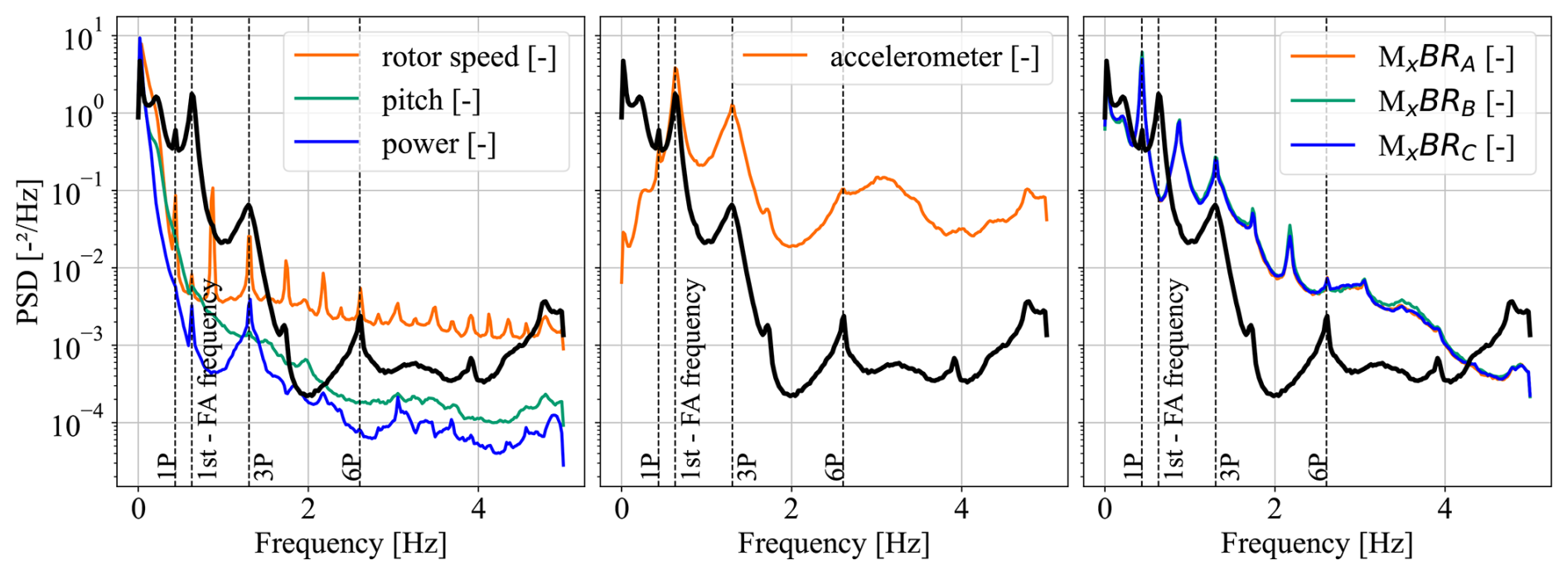
Figure 4 Normalized power spectrum density (PSD) of the possible input signals to be used in the training of a time series virtual load sensor: SCADA (left), nacelle accelerometer (middle), and blade root bending moments (right). The black line is added in all charts, as is the target variable M_fore−aft of the virtual load sensors. Normalization is based on the 10 min instance mean and standard deviation of the signal. The spectrum is generated by averaging 100 instances at rated wind speed (14 m s⁻¹). The dashed vertical lines indicate the rotor frequency (1P), the blade passing frequency (3P), and the higher harmonics and first fore–aft (FA) tower resonance.

However, only the accelerometer input signal can effectively capture the first fore–aft turbine frequency (around 0.62 Hz; Rinker et al., 2018), present in the target variable M_fore−aft, while its amplification of higher-frequency components compared to M_fore−aft is not considered pure electrical noise. When testing in standstill/parked conditions, there is a strong attenuation similar to that of the M_fore−aft PSD. The most consistent explanation is that the gearbox operation feeds high-frequency broadband vibrations to the nacelle accelerometer mounted below the bed plate near the gearbox. Virtual load sensors trained on the nacelle accelerometer might add higher-frequency oscillations to the M_fore−aft estimate, as shown in Fig. 8. The performance metrics selected are the normalized root mean square error (NRMSE), which is normalized by the standard deviation, σ_y, instead of the mean signal to avoid overshoot in the case of small mean values. To validate fatigue lifetime estimates, the damage equivalent load (DEL) and P_eq are analyzed in terms of the mean absolute error (MAE).

$$\begin{array}{}\text{(17)}& {\displaystyle }\text{NRMSE}={\displaystyle \frac{\mathrm{1}}{{\mathit{\sigma }}_y}}\sqrt{{\displaystyle \frac{{\sum }_{i=\mathrm{1}}^N(Y_{\mathrm{pred},i}-Y_{\mathrm{meas},i}{)}^{\mathrm{2}}}{N}}}\text{(18)}& {\displaystyle }{\text{MAE}}_{\mathrm{Load}=(\mathrm{DEL},P_{\mathrm{eq}})}={\displaystyle \frac{\mathrm{1}}{N}}\sum _{i=\mathrm{1}}^N\left|{\displaystyle \frac{{\text{Load}}_{\mathrm{pred},i}-{\text{Load}}_{\mathrm{meas},i}}{{\text{Load}}_{\mathrm{meas},i}}}\right|\end{array}$$

Here Y_pred is the time instant prediction, Y_meas is the measured value of M_fore−aft, and N is the number of instances evaluated.

5 Results

5.1 Continual calibration routines

Figure 5 shows the identified calibration factors for each of the two tower bottom strain gauges and the six blade root strain gauges, all converted to bending moments, as explained previously in Sect. 4.1. The charts to the right in both Fig. 5a and Fig. 5b show that the sensor position represents the angle difference of the installed sensor with respect to the SCADA reference variable, the yaw angle γ for the tower (cardinal north as the zero point), and the azimuth angle φ for the blade sensors (blade A upward as the zero point). Automatic routines manage to identify the position of the sensors correctly with a standard deviation (SD) of less than 4°, even though the azimuth correction explained in Appendix A was not applied at this stage, leading to higher variability before 2018 and after 2022.

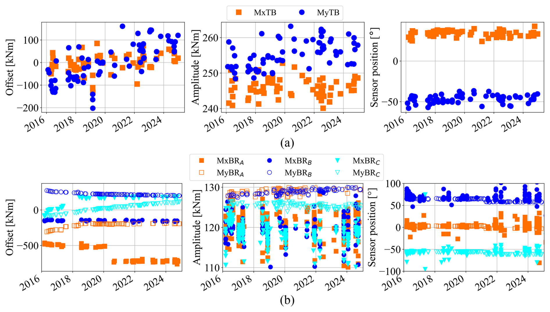
Figure 5 Identified calibration factors from 2016 to 2024 (inclusive), including offset (left), amplitude (middle), and sensor position (right) of strain gauges installed in the (a) tower bottom using yaw sweep routines and (b) blade root using low-speed idling (LSI) routines. The position of the tower bottom strain gauge bridge is defined with respect to the yaw angle γ(t). The position of the blade root strain gauge bridge is defined with respect to the azimuth angle φ(t). (a) Note that the mean offset value has been subtracted from each strain gauge bridge in the tower bottom for clarity, with a mean of 1240 and −3326 kNm for M_xTB and M_yTB, respectively.

From the left charts, it is possible to observe larger zero drifts for the blade root compared to the tower bottom strain gauges. M_xBR_A, M_yBR_A, and M_xBR_C also present an abrupt change in the zero drift in 2018 and 2020. This could be justified by sensor replacement or data acquisition settings; however, no final explanation has been validated. The amplitude (middle charts) in this method is the maximum gravitational overhang bending moment. In the case of the yaw sweep, it is driven by the rotor-nacelle weight with respect to the tower bottom (Faria et al., 2024), and for the LSI, it is driven by the blade weight with respect to the blade root (Faria et al., 2025). To have a quantitative accuracy quantification of the automatic routines in identifying the offset and the amplitude, their unexplained variability are normalized by reference values: the mean M_fore−aft bending equal to 3540 kNm for the tower strain gauge and the mean $M_{{\mathrm{flapwise}}_{(\mathrm{A},\mathrm{B},\mathrm{C})}}$ bending equal to 500 kNm for the blade strain gauges, both at rated wind speed. From the middle chart in Fig. 5a, an amplitude standard deviation of less than 4 kNm (equal to 0.04 MPa) can be observed for both sensors, which represents a variability of 0.1 % to the tower reference, while for the blade, an amplitude SD of less than 3 kNm can be seen, representing a 0.6 % variability. The larger variability from the blade root strain gauge calibration factors could be explained by the fact that its Wheatstone bridge is corrected for temperature differences in the whole blade but not for temperature gradients between the two blade surfaces. Once the offsets, shown in the left charts, are used to remove the artificial zero drift from the sensors, there will still be residuals that are not explained by the automatic routine. The offset residuals of the tower showed an SD of less than 60 kNm (corresponding to 0.5 MPa), which is 1.6 % of the reference, while, for blade strain gauges, the offset residuals had an SD of less than 10 kNm, representing a variability of 2 %.

5.2 Fatigue lifetime of tower and main bearings

Once all strain gauges have been calibrated and high-frequency measurements and SCADA are available, the long-term lifetime can be estimated over time, as shown in Fig. 6. Considering that failure is reached at unity, the basic lifetime of the main bearing L₁₀ can be evaluated using Eq. (7).

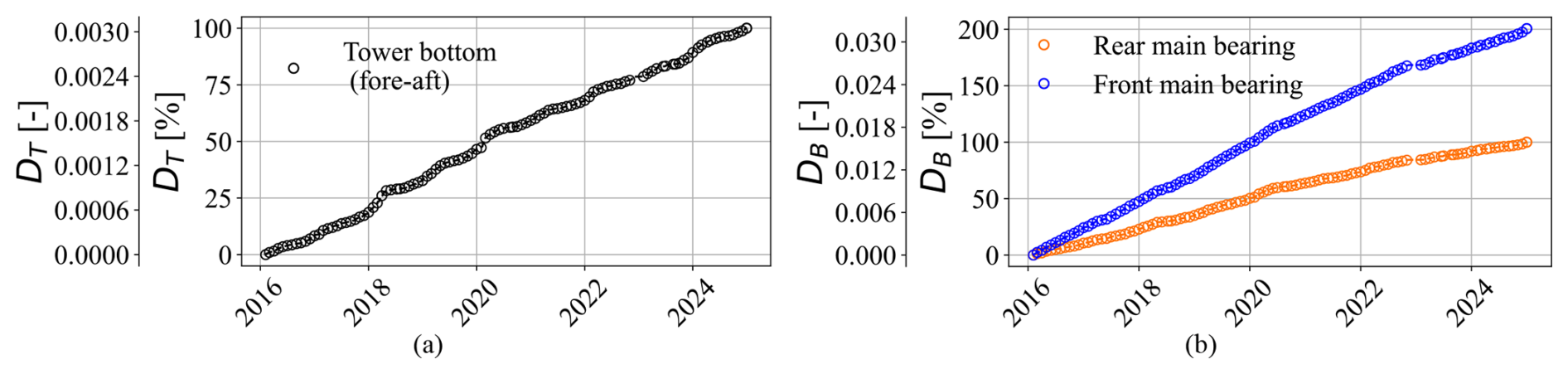
Figure 6 Fatigue damage accumulation of (a) the tower (structural component) and (b) the main bearings (rotating components) of the DTU research V52 turbine from 2016 to 2024 (inclusive). Fatigue damage was counted according to Eqs. (2) and (7). Charts have an absolute accumulation and a normalized y axis with respect to the end measured accumulated damage (D_B is normalized based on the rear main bearing).

The front bearing L_10,f is 282 years, and the rear bearing L_10,r is 566 years. Similarly, the tower has an even larger lifetime of 2952 years. This significantly longer lifetime, compared to the design lifetime of 20 years proposed by IEC 61400-1 (2019), is in part justified by the low wind potential of the Risø site, as discussed in Sect. 3. However, it also points to the fact that older and smaller turbines, such as the DTU research V52 turbine, have long remaining useful lifetimes (RULs) of key components that should be considered in lifetime extension (LTE) decisions.

5.2.1 Linear zero-drift assumption and simple uncertainty propagation to tower and main bearing lifetime

It is proposed to assume linear zero drift of the different strain gauge offsets as a single linear function or a combination of linear functions, which can be derived from continuous calibration factors over time. It is then important to quantify the uncertainty of this assumption in the life of the main bearings, which is based on the absolute load values P. The analysis was carried out by fitting the linear functions to the offsets and storing the residuals of the fit. Representative 10 min instances (DLCs 1.2, 3.1, and 4.1) were used to estimate the main bearing rating lifetime L_10,j, assuming an offset with Gaussian distribution derived from the residuals from the fitting function. A total of 10 000 Monte Carlo iterations were then carried out, calculating L_10,j based on a random selection of the offset Gaussian distribution. For all three instances, the standard deviation of both bearings L_10,j was below 0.7 %. Similar analysis was carried out for the fore–aft fatigue load DEL, and even negligible standard deviation was found. Fatigue is not affected by the mean load value (as described in Eq. 2) and is therefore not sensitive to the offset, assuming there are no large yaw angle variations within 10 min instances; see Eq. (9).

Effect of periodic calibration on the main bearings L₁₀

Now that continuous calibration with linear zero drift has been defined as the benchmark with an error of less than 1 %, it is sought to understand how the periodic calibration of strain gauges, as often carried out in industry, can influence the lifetime estimation of main bearings for this methodology. Table 2 shows the difference between the L₁₀ measured from 2016 to 2024 (inclusive) with continual calibration compared to periodic calibrations. The absolute results of the L₁₀ error due to calibration periodicity are not generalizable, as they are influenced by the zero-drift behavior of each monitoring setup and the loads of the wind turbine. However, it highlights that poor strain gauge calibration influences the lifetime estimation of main bearings for this methodology.

Table 2 Error in the L₁₀ estimation from 2016 to 2024 (inclusive) as a function of how often strain gauges are calibrated.

5.3 Virtual load sensor performance validation

A 160 h training dataset was used, as no significant improvements were found by enlarging the dataset, while downsampling from 50 to 10 Hz remained within the error convergence. The latter could decrease the dynamic content and underestimate the measured fatigue damage; therefore, to verify this, a procedure proposed by D'Antuono et al. (2023) was carried out, and sampling frequencies lower than 8 Hz contained more than 98 % of the measured fatigue damage in representative instances across all considered DLCs. A sampling frequency of 10 Hz is used.

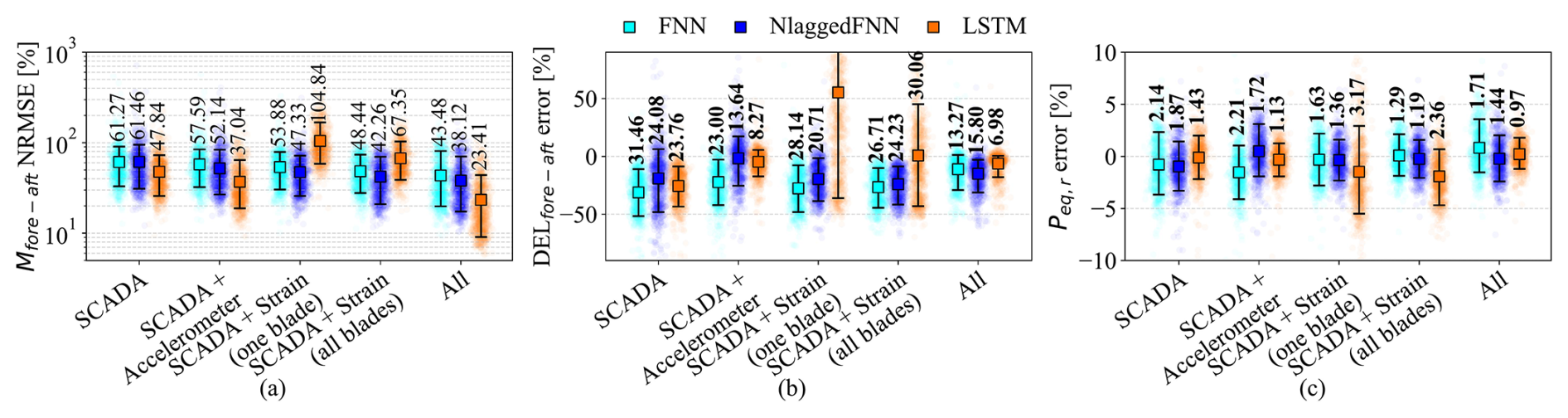
Figure 7 Virtual load sensor validation performance applied to 160 h of measurements. Their performance is shown based on the three metrics described in Eqs. (17) and (18). The different columns represent the feature selected as inputs and the different colors the model type (neural network architecture). The boxplots show the mean value and the 10th and the 90th percentiles. The numbers in the left subplot are the mean values of the NRMSE, whereas the bold values in the middle and right subplots are the mean absolute error (MAE).

The 15 different combinations of virtual load sensors (five input options and three model types) are validated using 160 h of data from 2019, also selected using the K-means clustering technique. From left to right, Fig. 7 presents all combinations of models tested in terms of the metrics shown in Eqs. (17) and (18), including NRMSE M_fore−aft (a), MAE DEL_fore−aft (b), and MAE P_eq (c). Raw data are added for completeness as transparent markers. The LSTM model with “all” inputs outperforms the other models significantly when comparing NRMSE. The mean error of 23 % is almost half that of the second-best-performing model combination (LSTM and “SCADA + accelerometer”), which yields 37 %. However, when no accelerometer signal was included and blade strain gauges were added, the LSTM model's performance worsened compared to the FNN and NlaggedFNN models. The LSTM added unrealistic oscillations in the time series estimate with larger 1P, 2P, and 3P frequency contributions and underpredicted the first FA frequency contribution, most likely due to poor model coupling of the blade strain gauges and azimuth angle φ inputs. NlaggedFNN was chosen when no accelerometer was available in the input. Regarding the equivalent load of the main rear bearing P_eq,r, influenced by the thrust estimate from the virtual load sensors, a negligible difference is observed between all combinations of models. Models with only SCADA reached MAE errors of 2 %. For the deployment from June 2017 to 2024, all models had an error below 10 % compared to the measured main bearing L₁₀ lifetime.

For the damage equivalent loads at the tower bottom fore–aft (DEL_fore−aft), models solely using SCADA had a minimum MAE error of 23.76 %. Looking at Fig. 8, it can be observed that the model with SCADA (LSTM) had an overprediction for very low-amplitude cycles, while it had an underprediction for larger-amplitude cycles. This becomes more predominant for conditions above rated wind speed (refer to Fig. 8b). Looking at its PSD, the model also does not properly capture the frequency components of the reference signal M_fore−aft. Adding the accelerometer yielded strong improvements. The best-performing combination with “SCADA + accelerometer” and LSTM had an MAE of 8.27 %, very close to the overall best-performing combination of “all” and LSTM with 6.98 %. The models that included strain without an accelerometer included undesired, sharp, and narrow-band peaks, most likely coming from the blade modes, which are not transmitted to the tower in reality; see Fig. 8 “SCADA + strain” (one blade or all blades).

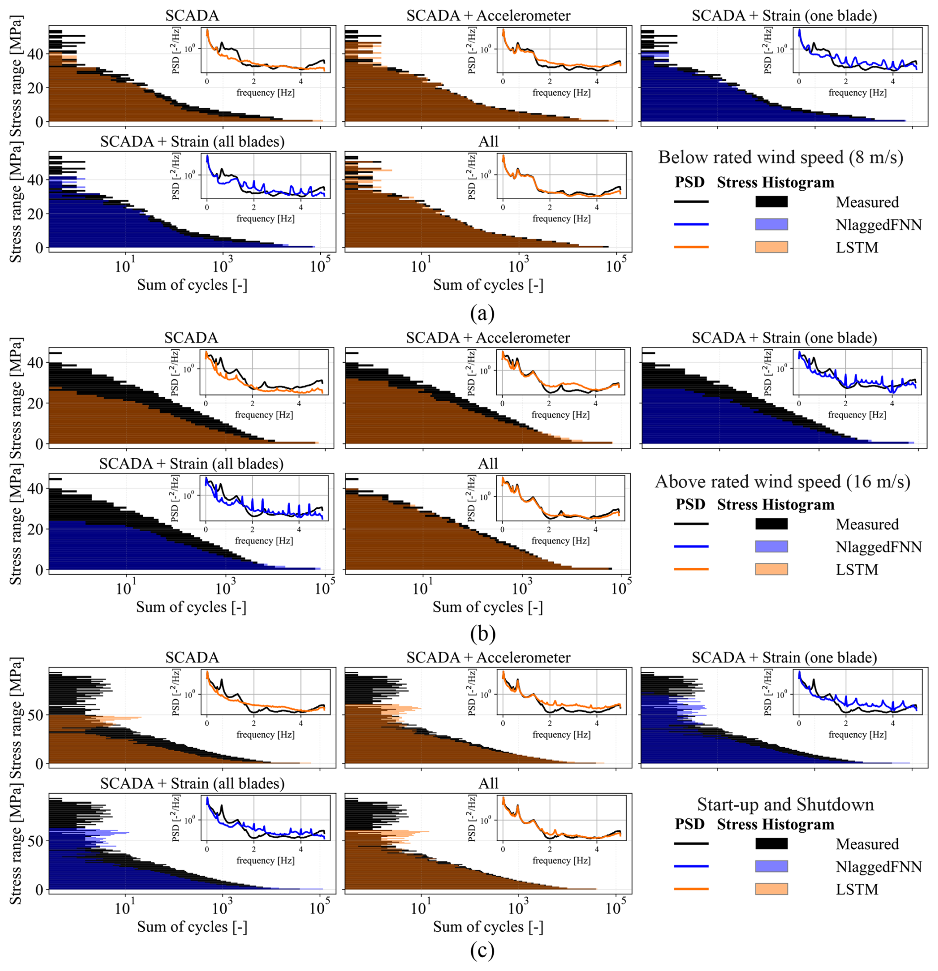
Figure 8 Stress cycle histogram and power spectrum density (PSD) chart (inset top right) of tower bottom M_fore−aft estimate for the different input signals combined with their best-performing model compared to the measurements (black). All stress histograms are the summation of, and the PSD charts the averaging of, 100 instances from 2019. (a) Below rated wind speed, 8 m s⁻¹ (DLC 1.2). (b) Above rated wind speed, 16 m s⁻¹ (DLC 1.2). (c) Start-up and shutdown (DLCs 3.1 and 4.1).

Looking closely at the two best-performing model combinations overall, “SCADA + accelerometer” and “all” with LSTM, it is worth taking a closer look at Fig. 8a and b. It is observed that only the model “all” is consistent in predicting stress ranges at both below and above rated wind speed, while rarely overpredicting the energy content for frequency components above 0.62 Hz. However, as shown in Fig. 8c for DLCs 3.1 and 4.1, all possible combinations underpredict large stress ranges, probably due to the lack of downwind oscillations from the blade root strain gauges once the blade is fully pitched.

5.4 Tower fatigue estimation using virtual load sensors

LSTM is chosen as the best model to combine with “SCADA”, “SCADA + accelerometer”, and “all”, while NlaggedFNN is chosen for “SCADA + strain” (one and all blades). The long-term deployment of these is performed to verify their reliability in estimating tower fatigue. Since the high-frequency database before June 2017 is sampled at 35 Hz, in contrast to 50 Hz after June 2017, the results related to the implementation of virtual load sensors do not include the 35 Hz dataset. Downsampling from 35 to 10 Hz requires interpolation, which may affect consistency. Figure 9 shows the accumulated tower fatigue damage of each virtual load sensor combination D_T normalized by the final accumulated damage. It is interesting to note that more damaging contributions are present at the beginning of each year because the Danish winter has higher wind speeds. All combinations of models underpredicted the accumulated damage (under-conservative), which is expected by looking at the analysis performed during validation and is shown in Fig. 8. The difference between the best-performing model “all” and the second-best model “SCADA + accelerometer” is equal to 11 %, from 64 % to 75 %. The remaining three models perform considerably worse in the long term, with estimates below 30 % of the reference damage.

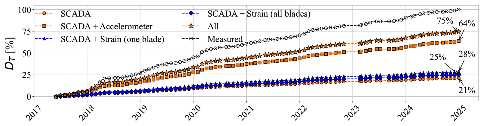
Figure 9 Tower bottom fore–aft fatigue damage accumulation comparison between different virtual load sensor models. It shows the total accumulation from June 2017 to 2024 (inclusive) normalized, for the sake of comparison, by the final measured fatigue accumulated damage. The different model combinations are shown by inputs used (marker) and by model type (marker fill color). The latter, for the sake of consistency, maintains the colors from Fig. 7 – blue for NlaggedFNN and orange for LSTM.

5.4.1 Proposed experimental slope correction for tower damage accumulation and statistical uncertainty

If a virtual load sensor is consistent throughout the majority of operating conditions over the year, it would underestimate different years with a similar error. Figure 10a shows the comparison for a full year (2018 as the first round year available) of estimated and measured accumulated damage. The slope η_k represents the underprediction ratio, calculated as the linear-fit slope between the estimated and measured accumulated damage yearly. Then, one could have accumulated damage from the virtual load sensor adjusted by the yearly slope as in

$$\begin{array}{}\text{(19)}& D_{\mathrm{T},\mathrm{a}}={\displaystyle \frac{D_{\mathrm{T},\mathrm{vls}}}{{\mathit{\eta }}_k}},\end{array}$$

where D_T,vls is the original and D_T,a is the adjusted accumulated damage of the virtual load sensor. The slope η_k is the linear-fit slope between the virtual load sensor and the measured damage for a given year k, and it is used as a correction factor.

The proposed experimental correction is the error associated with the choice of a given year k to calculate the slope by chance. Figure 10b shows the calculated η_k for each year. Note that small differences in annual mean wind speed were measured (see Sect. 3). The “all” and “SCADA + accelerometer” models have slopes that are closest to unity compared to the remaining models, while the first model has the lowest variability. Figure 11 attempts to evaluate the uncertainty by individually calculating the slope correction factor for each year from 2018 to 2024 (inclusive) and adjusting the expected accumulated damage of the two best-performing virtual load sensors by the average slope ${\mathit{\eta }}_{\mathrm{avg}}=\mathrm{1}/N\cdot {\sum }_k^N{\mathit{\eta }}_k$ (where N is the number of years) and the annual slope variability with the standard deviation (SD) and minimum/maximum values. The slope variability could be driven by annual wind statistics and model performances (see Fig. 8). To reach an estimated SD accuracy of ±10 % with limited samples and with a confidence level of 90 %, more than 100 samples are required, considering a Gaussian distribution (Schillaci, 2022). Since our available N is low (7 years), both the SD and the maximum/minimum bounds are evaluated. The model “all” with LSTM has the shortest error convergence time, nearly within 6 months, and has a mean error for the adjusted accumulated damage equal to −1.8 % and variability within 3.5 % and −6.5 %. The second-best-performing model “SCADA + accelerometer” with LSTM has a mean error of −4.2 % and a variability bounded within 13 % and −15 %. The remaining virtual load sensors are not shown, since they capture the PSD and the stress range distribution in a less consistent manner.

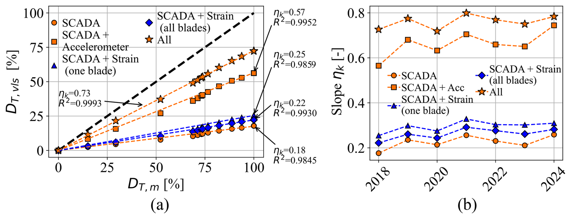
Figure 10 (a) Comparison between accumulated damage from virtual load sensors (D_T,vls) and measured damage (D_T,m) for 2018. The slope η_k of each model refers to the linear-fit slope, while R² refers to the coefficient of determination (markers are shown once per month). (b) The slope η_k calculated for each full year k. Blue for NlaggedFNN and orange for LSTM.

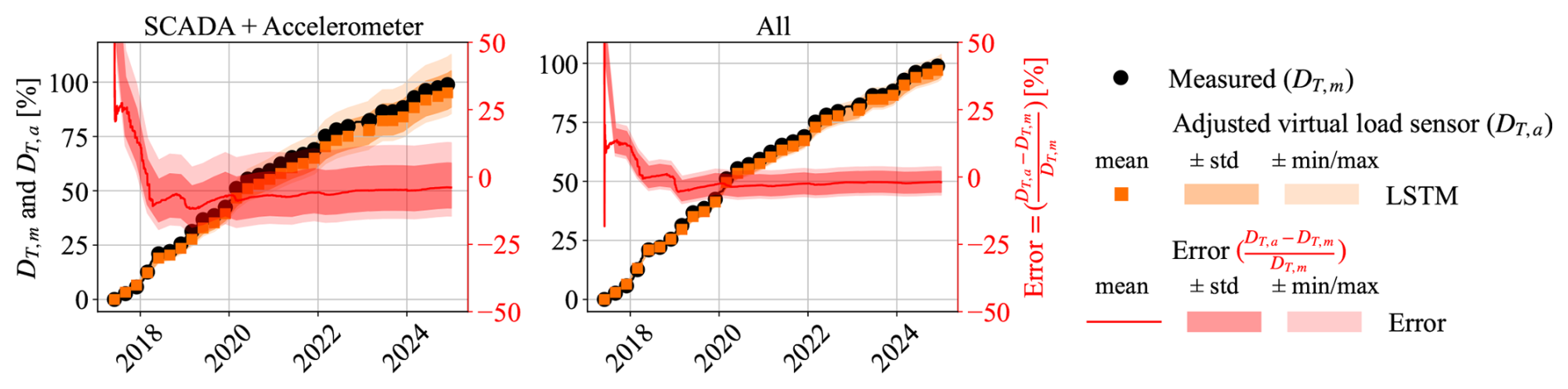
Figure 11 Measured D_T,m and adjusted D_T,a damage accumulation of the virtual load sensors based on the yearly slope correction is shown. The two best-performing models are shown. The damage adjusted by the average slope value from 2018 to 2024 (inclusive) is shown as the markers. The filled areas represent the variation around the standard deviation (inner) and bounded between the maximum and minimum values observed (outer). The error between the virtual load sensor and measured damage accumulation is shown on the right red y axis.

The experimental slope correction results should not be seen as fully validated but as a trial to adjust models that consistently capture the dynamic content of the tower bottom while underpredicting the peaks and valleys, leading to stress range underprediction.

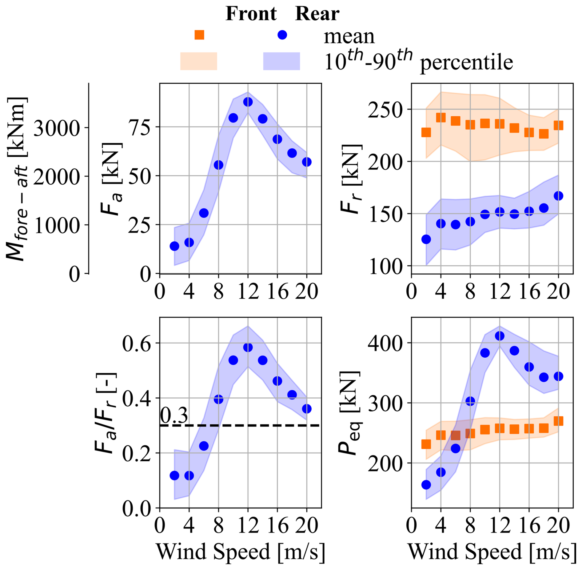
Figure 12 Front and rear main bearing loads as a function of wind speed. The obtained axial load F_a as a function of the tower bottom bending moment M_fore−aft, the radial load F_r, the ratio with the rear bearing limiting factor, and the dynamic equivalent load P_eq are presented. The mean value is represented by the marker, while the 10th–90th percentiles are represented by the filled area from 2016 to 2024 (inclusive).

5.5 Main bearing loads and fatigue lifetime analysis

As detailed in Sect. 2.2, the main bearing life is calculated directly from the applied radial and axial loads. The axial load of the main bearing F_a is linearly linked to the tower bottom bending moment as in $F_{\mathrm{a}}=M_{\mathrm{fore}-\mathrm{aft}}/h$, where h is the height difference between hub height (44 m) and the height of the sensor (3.787 m). Here, M_fore−aft is assumed to be representative of the turbine thrust curve. The radial load of the main bearings F_r is equal to the estimated F_r,f (front) and F_r,r (rear), respectively. For a more detailed explanation, see Sects. 3 and 4.2. The 10 min mean loads are shown in Fig. 12 as a function of wind speed. The front and rear bearings F_r have different behavior with respect to the wind speed. The front main bearing has a fairly flat distribution at higher load, while, for the rear main bearing, the radial load increases incrementally. The $F_{\mathrm{a}}/F_{\mathrm{r}}$ ratio for the rear main bearing is almost entirely above the limiting factor, which will worsen the estimated rating life, as the Y factor increases (see Eq. 4). Finally, P_eq of the front bearing has a slight positive trend, most probably due to higher rotor speeds at higher wind speed, while the rear bearing's dynamic equivalent load is driven by the axial load F_a. A similar analysis, shown in Fig. 9, was performed for the main bearing fatigue damage, D_B, with the five best virtual load sensor combinations yielding errors below 2 %, likely because bearing fatigue is dominated by the mean P_eq rather than load fluctuations in the radial F_r and axial F_a loads. Further investigations focus on the tower fatigue damage, D_T.

5.5.1 Sampling frequency and gearbox mounting stiffness assumptions

Before moving on to the long-term results, it is important to verify some of the assumptions made in this work. As in the fatigue estimation of the tower bottom, P_eq and L₁₀ were calculated based on measured data downsampled from 50 to 10 Hz. At 10 Hz, there will be a mean error of less than 2 %, with a 10th–90th percentile within 5 %.

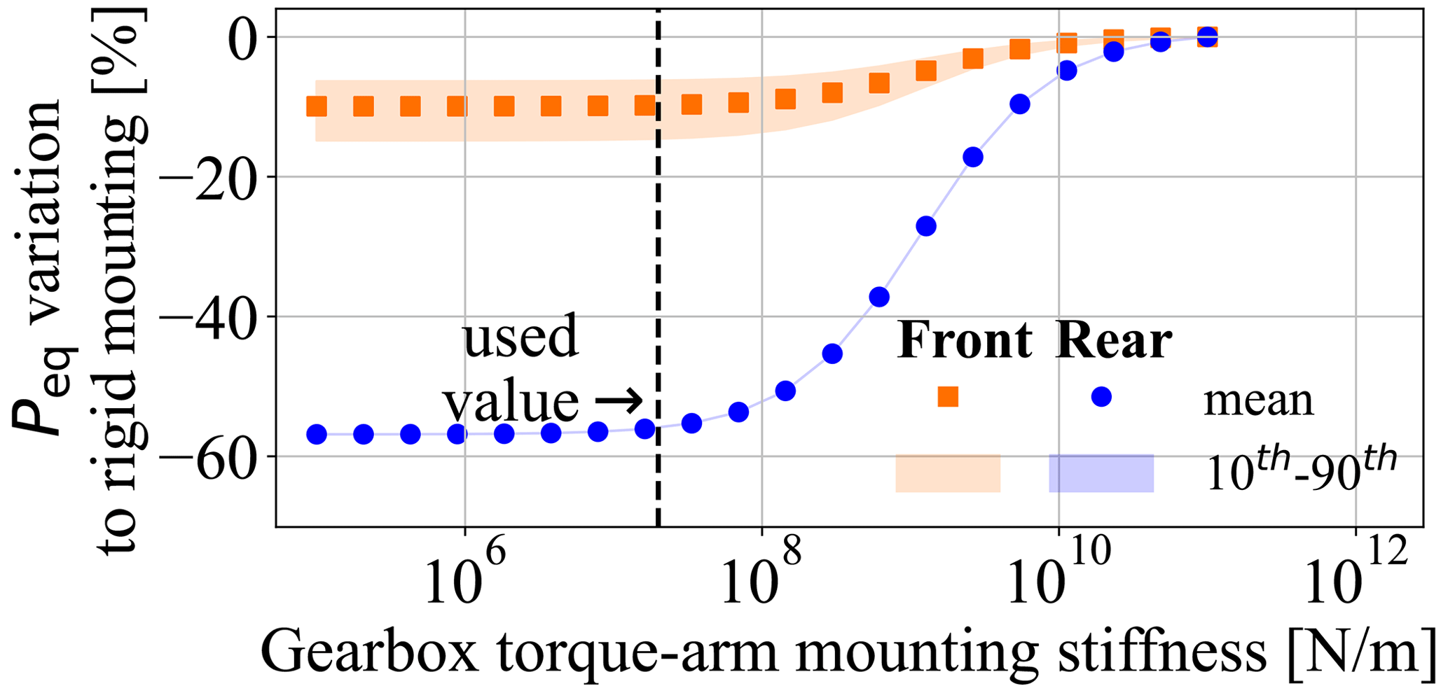
Figure 13 Results of sensitivity analysis of the stiffness of gearbox mounts on the main bearing dynamic equivalent load P_eq based on a 160 h randomly selected dataset. The value used (dashed black line) for the gearbox mounting stiffness refers to a stiffness of 20×10⁶ [N m⁻¹], close to the literature values found in Haastrup et al. (2011) and Keller et al. (2016).

Figure 13 shows the effect of the stiffness used to model the gearbox mounting fixation points on P_eq of the front and rear main bearing. A small variation is observed if the stiffness is neglected or used as in the literature (Haastrup et al., 2011; Keller et al., 2016). However, as shown in Fig. 13, an overprediction of 10 % and 60 % of the front and rear dynamic equivalent loads P_eq could be reached if a gearbox is rigidly fixed in a four-point drivetrain, which is not a realistic assumption.

5.5.2 Environmental and operational condition (EOC) mapping of the main bearing dynamic equivalent loads P_eq

The main bearing P_eq was mapped with the environmental conditions of each mean 10 min instance to visualize potential patterns. Figure 14 confirms the intuitive reasoning that the equivalent loads of the front main bearing P_eq,f are driven more by the static gravitational load of the rotor. However, P_eq,f still contains almost 10 % fluctuations due to the shear exponent from 0.05 to 0.15 in all wind ranges and a similar turbulence effect at rated wind speed. In a different manner, for the rear main bearing, the turbine thrust curve dictates the value of P_eq,r.

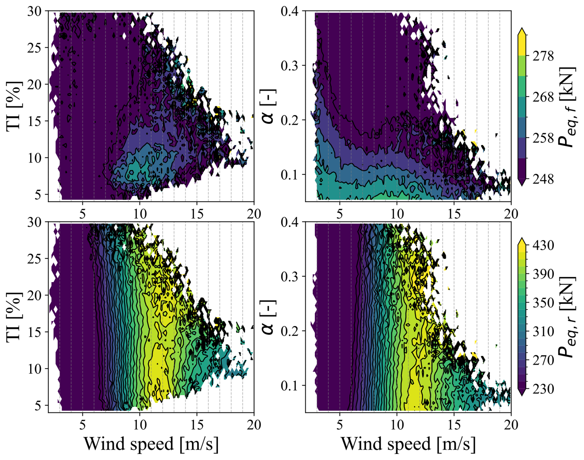
Figure 14 Equivalent dynamic loads of the front P_eq,f (top) and rear P_eq,r (bottom) main bearings of the DTU research V52 turbine mapped as a function of wind speed, turbulence intensity (TI), and shear exponent α. The measurement period covers 2016 to 2024 (inclusive).

Looking closely at P_eq,f, the results resemble Kenworthy et al. (2024) for a three-point drivetrain for the effect of lower shear on increased bearing loads. A comparable effect of low turbulence is found at rated wind speed. An increase of 10 % in P_eq,f loads (from 248 to 268 kNm) can be seen in the rated wind speed for the turbulence values of 15 % to 10 %. A similar load increase is observed for shear exponents of 0.15 to 0.08 at rated wind. In terms of the load on the rear main bearing P_eq,r (locating), low turbulence can exceed the shear influence at rated wind speed, as also suggested by the HIPERWIND D5.4 (2024) report. This is a result of keeping the level of axial load F_a at the peak of the thrust curve. There is an approximately 10 % increase in load, driven by a change in turbulence from 15 % to 8 %. The peak of the thrust curve is claimed to be the main driver of the fatigue load in the locating bearing P_eq,r (Kenworthy et al., 2024; Quick et al., 2025). However, Fig. 14 highlights the effect of the low turbulence intensity at rated wind speed, referring to the most damaging operating condition mapped, and that should affect the lifetime of the main bearing more severely depending on the probability of occurrence, as described in Eq. (6). To explain this observation, Fig. 15 shows a simplified representation of the increase in fatigue load of a locating main bearing at low turbulence. Wind speed is defined as a normal distribution with a mean value at rated U_rated, the peak of the thrust curve, and a standard deviation σ defined by $\text{TI}=\mathit{\sigma }/U_{\mathrm{rated}}$. The dynamic load P is calculated according to Eq. (4), and the axial load F_a has been replaced by a scaled thrust curve of a reference wind turbine (Bak et al., 2013) in order to have a complete curve below and above rated conditions. A decrease from 20 % to 10 % in TI in the wind speed distribution increased the mean dynamic load $\overline{P}$ of the rear main bearing in the DTU research V52 turbine by nearly 10 %. Similar results were observed for P_eq,r in Fig. 14. This effect arises from the turbulence averaging of the dynamic load P, as expressed in the following equation:

$$\begin{array}{}\text{(20)}& \overline{P}=\int p_{\mathrm{N}}\left(U\right)\cdot P\left(U\right)\mathrm{d}U,\end{array}$$

where $\overline{P}$ is the mean of the dynamic load P, p_N is the normal distribution that represents the wind speed, and P(U) is the dynamic load P as a function of the wind speed U.

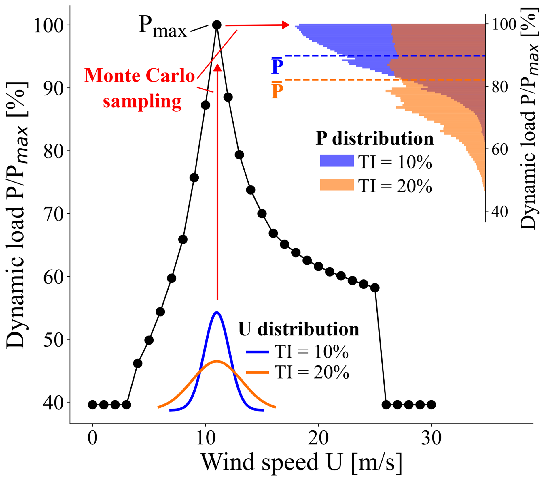
Figure 15 Conceptual representation of the effect of turbulence intensity (TI) at rated wind speed on the wind speed distribution U, modeled as a normal distribution (see bottom inset), and its influence on the dynamic load P distribution on the rear main bearing of the DTU research V52 turbine (see top-right inset). In this simple exercise, the turbine thrust values are derived from a simplified DTU 10 MW (Bak et al., 2013) thrust curve scaled to the DTU research V52 turbine by the maximum axial load F_a, as shown in Fig. 12, in order to generate a representative and complete thrust curve. Monte Carlo sampling is used with 10⁶ samples to generate the P histogram. The numerically obtained mean dynamic load $\overline{P}$ can also be calculated using Eq. (20) at rated wind speed and is shown as horizontal dashed lines.

5.5.3 Main bearings L_10 m and a_ISO

Applying the drivetrain thermal model, consistent temperature ranges were found for the normal operating conditions (DLC 1.2) of the main bearings. The temperatures of the front and rear main bearings had minimum, mean, and maximum values of 8, 34, and 55 and 18, 40, and 61 °C, respectively, while the viscosity ratio κ had minimum values of 0.84 and 0.64, respectively. The gearbox temperature model yielded 3 °C MAE, which is reasonable considering the scope of this investigation.

The seasonal variation corresponded to approximately ±10 °C in the front bearing and ±8 °C in the rear bearing temperatures, while the operational variability reached around ±15 °C variation in the front and ±20 °C in the rear bearing temperatures. The results of such environmental and operation conditions (EOCs) can be visualized in Fig. 16, assuming a severe level of grease contamination. The grease cleanliness affects the parameters' ability to estimate the variable contamination factor e_c, which by consequence affects a_ISO (ISO-281, 2007). This assumption represents a worse scenario in which re-greasing of the main bearings is not performed in the long term, as suggested by the manufacturers. Figure 16 highlights the large impact of the ambient temperature on the modified rating lifetimes of main bearings, in which there is no nacelle temperature control. For the rear main bearing, even for such an overdesigned bearing, at rated wind speed with low TI or with ambient temperatures above 20 °C, the bearing lifetime is reduced to below the design lifetime of 20 years. In addition to that, once a_ISO is considered, it seems that turbulence overcomes shear as the most influential factor for the rear main bearing at rated wind speed.

Figure 16 The modified rating life of the front L_10 m,f (top) and rear L_10 m,r (bottom) main bearings of the DTU research V52 turbine as a function of wind speed, turbulence intensity (TI), shear exponent α, and ambient temperature T_amb, together with pointers to the rear T_r and front T_f main bearing temperatures. It is assumed that there is a severe level of contamination for the grease lubricant. The latter represents a scenario in which re-greasing intervals recommended by the OEM are not followed. It is important to note that there are limits related to a_ISO implementation, as defined by ISO-281 (2007): at a_ISO=50, $e_{\mathrm{c}}{C}_u/P_{\mathrm{eq}}=\mathrm{5}$ (maximum bound), and viscosity ratio κ=0.1 (minimum bound), which has not been reached in this work. The lower limit of the color bar (yellow color) was chosen to match the turbine design lifetime of 20 years.

Significant variations can be observed in L_10 m due to EOCs, but it is important to mention that the grease cleanliness level should affect the bearing lifetime more severely (Kenworthy et al., 2024). Figure 17 shows on a logarithmic scale the distribution of a_ISO as a function of the assumed or inspected grease cleanliness in a wind turbine. In the worst-case scenario with “very severe contamination”, 70 % of instances are penalized, and $L_{\mathrm{10},\mathrm{r}}=\mathrm{566}$ years decreases to an $L_{\mathrm{10}\mathrm{m},\mathrm{r}}=\mathrm{200}$-year lifetime.

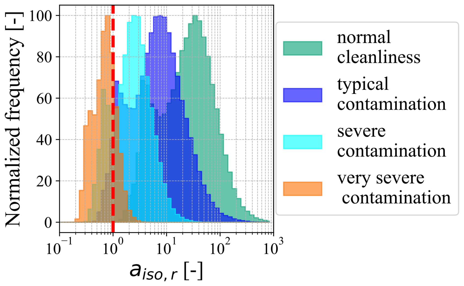
Figure 17 Normalized histogram showing the distribution of the rear main bearing life modification factor a_ISO,r as a function of the grease cleanliness levels. The dashed red line shows the limit for L₁₀=L_10 m. The bound of a_ISO<50 is not applied for the sake of clarity.

6 Conclusions

In this work, methods were investigated to allow for reliable lifetime counting of large load-carrying components, both structural in the form of a tower and rotating in the form of main bearings. The methodology was demonstrated using measurements from the DTU research V52 wind turbine for a continuous period of almost a decade.

The strain gauges at the bottom of the tower and the root of the blade were continually calibrated from 2016 to 2024 (inclusive) with at least 20 calibration instances per year. The yaw sweeps and low-speed idling (LSI) routines were verified for long-term calibration, and all strain gauges presented reliable behavior. We assumed linear behavior to model the zero drift of the strain gauges, which has to be validated by carrying larger case-study comparisons, accounting for different Wheatstone bridge configurations. However, it is interesting to observe that eight full strain gauge bridges from the DTU research V52 turbine have presented similar behavior over time, with low unexplained variability after the proposed correction.

Lifetime counting of a structural component, such as the tower, and other load-carrying components, such as main bearings, was carried out for almost a decade, without having design information from the blade or mid-fidelity aeroelastic models.

The use of virtual load sensors based on data-driven methods is promising in the field of wind energy, where structural health monitoring (SHM) campaigns can be expensive and take a long time. These could serve as a continuous high-frequency thrust estimate. In this work, counting 7.5 years of the fatigue lifetime of the tower bottom using a virtual load sensor yielded a damage prediction of 75 % of the best-performing model. It is interesting to highlight that a 1 % difference in MAE DEL between models with and without blade root strain gauges resulted in an 11 % difference in the lifetime estimation. After an experimental correction, assuming a year of available measurement data, the lifetime error was reduced to ±5 %. Future research could investigate minimum measurement periods for a reliable slope correction; assumptions on the training of the data-driven models, such as K-means clustering and the error function (de N Santos et al., 2024); and test cases that could bias the analysis. The results from this work might not be considered state of the art but can be seen as a discussion of the challenges of long-term and continuous deployment of virtual load sensors in wind turbines considering several DLCs.

Finally, the main bearing loads P_eq and modified lifetime L_10 m were mapped in terms of relevant environmental conditions and grease cleanliness. The first showed that a front main bearing in a four-point drivetrain has a longer life as the shear exponent increases, whereas the fatigue loads in the locating rear main bearing are dictated by the peak of the thrust curve and are larger at rated wind speed. The rear main bearing was observed to have a longer lifetime as the shear and turbulence intensity increase, which can be explained by the turbulence averaging of the thrust loads. Estimates of operating temperature and grease cleanliness (Kenworthy et al., 2024) were identified as key drivers in the modified rating lifetime L_10 m of the main bearings. Although the drivetrain thermal model resulted in realistic temperature ranges, validation with measurement values is the logical next step. Lubricant cleanliness corrections significantly affect predicted lifetime but have not been validated for large grease-lubricated bearings, unlike smaller bearings (Needelman and Zaretsky, 2014).

Appendix A: Azimuth angle correction for the DTU research V52 turbine

Figure A1 presents the problem and the solution applied to the azimuth angle sensor. For periods before 2018 and after 2020, the measured azimuth angles contained severe variations in regular patterns, which did not extend to variability in the edgewise bending moment M_edgewise of the blades. In this manner, such variations were triggered as a sensor malfunctioning. To correct for such an issue, an azimuth angle estimate φ_e was derived as a constant-gain blend between two complementary signals. The first signal is the measured azimuth angle φ_m sampled at 10 Hz, shown in Fig. A1 as the black line (left y axis). The second signal is the controller-defined rotor speed (SCADA) ω sampled at 10 Hz, which has a lower resolution, and is shown in the same figure as the red line (right y axis). The period Δt is defined as the inverse of the sampling frequency.

The correction method works by first identifying the best phase shift φ_r,0 of the azimuth angle in a 10 min instance, which is the initial point between the cumulative φ_m and ${\sum }_i{\mathit{\omega }}_i\cdot \mathrm{\Delta }t$, using a few sequential data points. The instantaneous angle based on the rotor speed will be ${\mathit{\phi }}_{\mathrm{r},i}={\mathit{\omega }}_i\cdot \mathrm{\Delta }t+{\mathit{\phi }}_{\mathrm{r},i-\mathrm{1}}$, for i>1, and ${\mathit{\phi }}_{\mathrm{r},i}={\mathit{\phi }}_{\mathrm{r},\mathrm{0}}$, for i=1. The final estimated azimuth is defined as ${\mathit{\phi }}_{\mathrm{e},i}={\mathit{\phi }}_{\mathrm{r},i}+K\cdot d$, if d<d_limit, and ${\mathit{\gamma }}_{\mathrm{e},i}={\mathit{\phi }}_{\mathrm{r},i}$, if d>d_limit . Here d is the difference between the measured instantaneous angle and the estimation of the rotor speed $d={\mathit{\phi }}_{\mathrm{m},i}-{\mathit{\phi }}_{\mathrm{r},i}$. The two manually tuned variables are the gain K and the distance limit d_limit. The first defines how reliable the fluctuations are from the measured azimuth. The latter correlates with the threshold of how many degrees the measured azimuth can realistically change within Δt. In this work, the parameters were tuned to K=0.1 and d_limit=30°. The validation was carried out in a good year (2019) by applying the method on 160 h of representative instances containing the design load cases (DLCs) 1.2, 3.1, and 4.1. The maximum instantaneous error $/{\mathit{\phi }}_{\mathrm{m}}-{\mathit{\phi }}_{\mathrm{e}}/$ was below 5°.

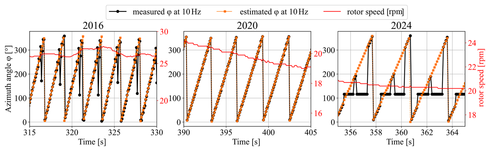
Figure A1 Representative examples of the azimuth angle in the SCADA from the DTU research V52 turbine showing problems with the measurement data acquired in 2016 and 2024. An estimated azimuth angle (orange) is obtained based on the controller SCADA rotor speed (red) and the measured azimuth angle (black).

Appendix B: Statically indeterminate system for a four-point drivetrain considering the gearbox mounting stiffness

Figure B1 shows the drivetrain schematic that allows one to derive the radial loads in the main bearings while considering the stiffness of the gearbox mounting, as shown in Fig. 3a. The vertical direction is chosen as it includes the most significant resultant loads (gravitational and aerodynamic), and the horizontal direction can be solved in the same manner. The static gravitational loads acting on the main shaft are derived from a combination of public sources and visual inspections of the turbine nacelle. The same applies to lengths (e.g., L_shaft). The gravitational force of the rotor F_rotor is calculated assuming a rotor and a hub mass of 10 t (third party source; see Scribd, 2021). The gravitational force of the shaft F_shaft assumes a shaft mass equal to 1 t, between an internal estimate of 0.8 t and the Fingersh et al. (2006) estimate of 1.2 t, which uses the best-fit equation $m_{\mathrm{shaft}}=\mathrm{0.0142}\cdot D^{\mathrm{2.888}}$ from historical data (given D as the rotor diameter in meters and the mass in tonnes).

The system of equations for the forces and bending moments for Fig. B1a is composed of

$$\begin{array}{}\text{(B1)}& {\displaystyle }\sum F=\mathrm{0}=-F_{\mathrm{rotor}}-F_{\mathrm{shaft}}+R_{\mathrm{f}}+R_{\mathrm{r}}+F_{\mathrm{g}},\text{(B2)}& {\displaystyle }\begin{array}{rl}\sum M(x=\mathrm{0})& =\mathrm{0}=-M_{\mathrm{v}}+M_{\mathrm{rotor}}+R_{\mathrm{f}}{L}_{\mathrm{1}}\\ & -F_{\mathrm{shaft}}{L}_{\mathrm{shaft}}+R_{\mathrm{r}}(L_{\mathrm{1}}+L_{\mathrm{2}})\\ & +F_{\mathrm{g}}(L_{\mathrm{1}}+L_{\mathrm{2}}+L_{\mathrm{3}}),\end{array}\end{array}$$

where the assumed sign conversion is upwards and counterclockwise as positive. The “top view” (Fig. B1b) has the same formulation – it is solved independently but without gravitational loads F_rotor, M_rotor, and F_shaft.

Since the system is statically indeterminate, there are two independent equations (Eqs. B1 and B2) and three unknown reactions, R_f, R_r, and F_g. To add a third equation, the main shaft is modeled as a flexible beam, with small deflections, linear material (Young's modulus E), and a second area moment of inertia I along the length, as explained by Budynas and Nisbett (2020).

Equation (B4) describes the bending moment as a function of beam deflection w along x through a double-integration step.

$$\begin{array}{}\text{(B3)}& {\displaystyle }\begin{array}{rl}\text{EI}{\displaystyle \frac{{\mathrm{d}}^{\mathrm{2}}w}{\mathrm{d}{x}^{\mathrm{2}}}}& =M=-M_{\mathrm{v}}+M_{\mathrm{rotor}}\\ & +F_{\mathrm{rotor}}\cdot x+F_{\mathrm{shaft}}\cdot \langle x-L_{\mathrm{shaft}}\rangle -R_{\mathrm{f},\mathrm{v}}\\ & \cdot \langle x-L_{\mathrm{1}}\rangle -R_{\mathrm{r},\mathrm{v}}\cdot \langle x-(L_{\mathrm{1}}+L_{\mathrm{2}})\rangle \end{array}\text{(B4)}& {\displaystyle }\begin{array}{rl}\text{EI}w=& -{\displaystyle \frac{M_{\mathrm{v}}}{\mathrm{2}}}\cdot x^{\mathrm{2}}+{\displaystyle \frac{M_{\mathrm{rotor}}}{\mathrm{2}}}\cdot x^{\mathrm{2}}+{\displaystyle \frac{F_{\mathrm{rotor}}}{\mathrm{6}}}\cdot x^{\mathrm{3}}\\ & +{\displaystyle \frac{F_{\mathrm{shaft}}}{\mathrm{6}}}\cdot \langle x-L_{\mathrm{shaft}}{\rangle }^{\mathrm{3}}-{\displaystyle \frac{R_{\mathrm{f},\mathrm{v}}}{\mathrm{6}}}\cdot \langle x-L_{\mathrm{1}}{\rangle }^{\mathrm{3}}\\ & -{\displaystyle \frac{R_{\mathrm{r},\mathrm{v}}}{\mathrm{6}}}\cdot \langle x-(L_{\mathrm{1}}+L_{\mathrm{2}}){\rangle }^{\mathrm{3}}+C_{\mathrm{1}}\cdot x+C_{\mathrm{2}}\end{array}\end{array}$$

Here 〈〉 is the Macaulay bracket or discontinuity function. To solve the constants C₁ and C₂ and generate a third independent equation, three known boundary conditions can be used as

$$\begin{array}{}\text{(B5)}& \begin{array}{rl}& w(x=L_{\mathrm{1}})=\mathrm{0},w(x=L_{\mathrm{1}}+L_{\mathrm{2}})=\mathrm{0},\\ & w(x=L_{\mathrm{1}}+L_{\mathrm{2}}+L_{\mathrm{3}})={\displaystyle \frac{F_{\mathrm{g}}}{K_{\mathrm{g}}}}.\end{array}\end{array}$$

Finally, once the constants are calculated, the third independent equation can be derived by applying a third known boundary condition (deflection at the gearbox $F_{\mathrm{g}}/K_{\mathrm{g}}$). The resultant third independent equation is then

$$\begin{array}{}\text{(B6)}& \begin{array}{rl}\text{EI}{\displaystyle \frac{F_{\mathrm{g}}}{K_{\mathrm{g}}}}=& -{\displaystyle \frac{M_{\mathrm{v}}}{\mathrm{2}}}(L_{\mathrm{1}}+L_{\mathrm{2}}+L_{\mathrm{3}}{)}^{\mathrm{2}}+{\displaystyle \frac{M_{\mathrm{rotor}}}{\mathrm{2}}}(L_{\mathrm{1}}+L_{\mathrm{2}}+L_{\mathrm{3}}{)}^{\mathrm{2}}\\ & +{\displaystyle \frac{F_{\mathrm{rotor}}}{\mathrm{6}}}(L_{\mathrm{1}}+L_{\mathrm{2}}+L_{\mathrm{3}}{)}^{\mathrm{3}}\\ & +{\displaystyle \frac{F_{\mathrm{shaft}}}{\mathrm{6}}}(L_{\mathrm{1}}+L_{\mathrm{2}}+L_{\mathrm{3}}-L_{\mathrm{shaft}}{)}^{\mathrm{3}}-{\displaystyle \frac{R_{\mathrm{f}}}{\mathrm{6}}}(L_{\mathrm{2}}+L_{\mathrm{3}}{)}^{\mathrm{3}}\\ & -{\displaystyle \frac{R_{\mathrm{r}}}{\mathrm{6}}}(L_{\mathrm{3}}{)}^{\mathrm{3}}+C_{\mathrm{1}}(L_{\mathrm{1}}+L_{\mathrm{2}}+L_{\mathrm{3}})+C_{\mathrm{2}}.\end{array}\end{array}$$

The complete derivation is omitted for conciseness, consisting primarily of algebraic manipulation and variable substitution. Using the three independent equations, (B1), (B2), and (B6), and assuming quasi-static equilibrium at each time instant, one can calculate the independent unknowns, R_f, R_r, and F_g, referred to in the main text as F_r,f, F_r,r, and F_g.

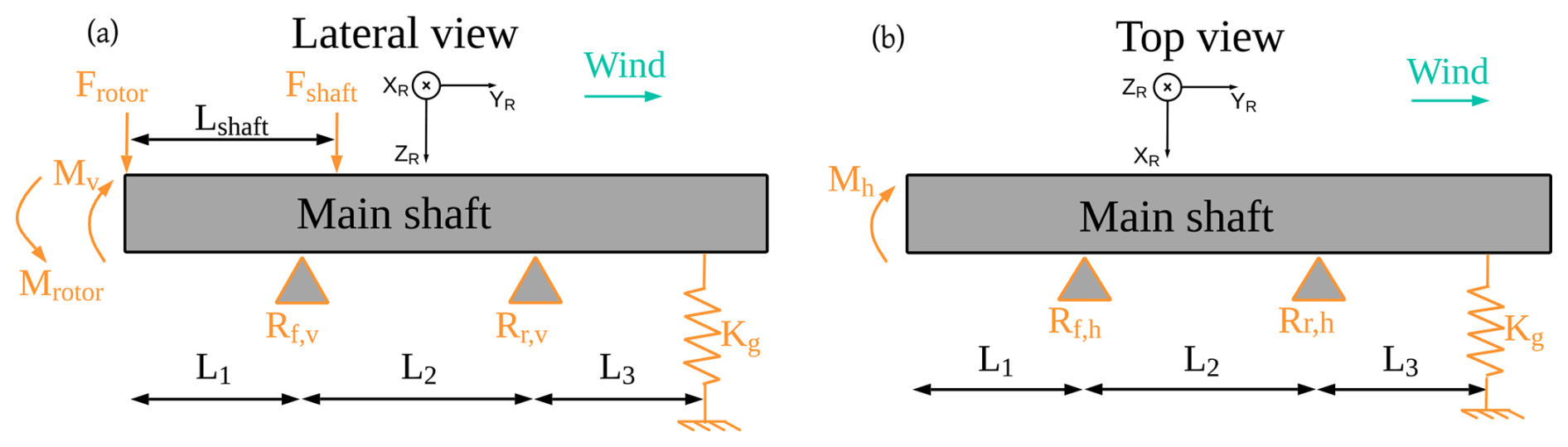
Figure B1 Drivetrain schematic used to represent the external loads applied and the supporting elements in the (a) lateral view and (b) top view, with respect to the rotor coordinate system XYZ_R. F_rotor and F_shaft are the rotor and shaft gravitational loads, respectively; L_shaft is the shaft center-of-mass distance; M_rotor is the bending resultant from the rotor weight F_rotor and L_hub, as the hub is not modeled (see Fig. 3); and M is the aerodynamical loading in the vertical direction. The main shaft is supported by the front R_f and rear R_r main bearings (referred to in the main text as F_r,f and F_r,r), in the vertical v and horizontal h directions. Lastly, it is supported by the gearbox through the equivalent spring K_g, which results in the force F_g.

Appendix C: Hyperparameter tuning of the data-driven virtual load sensors

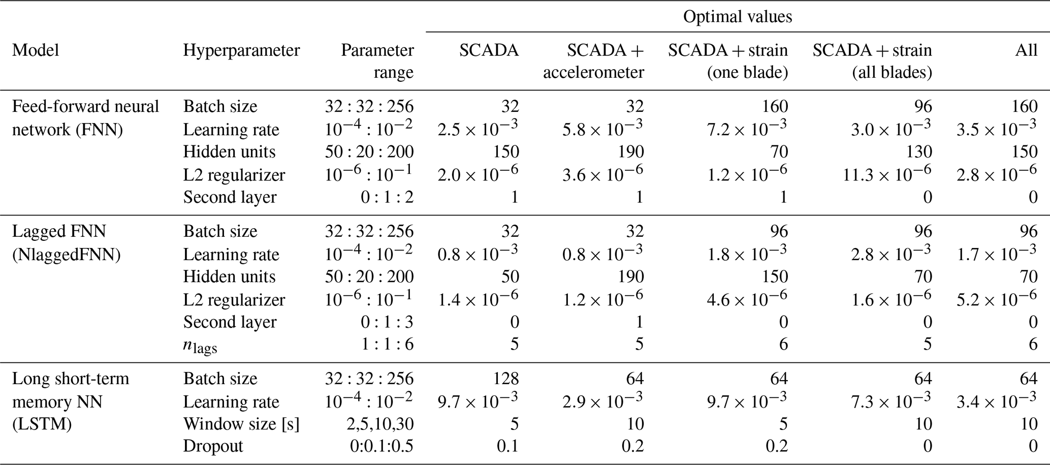
The models described in Sect. 4.3 are tuned using a random search tuner (O'Malley et al., 2019) to improve the model performance. Table C1 shows the hyperparameters' possible range and optimal value found for each virtual load sensor. Similarly to the methodology applied by Dimitrov and Göçmen (2022) and Gräfe et al. (2024), there are hyperparameters related to the data architecture, such as the number of lags n_lags in an NlaggedFNN and the window size in an LSTM, as well as hyperparameters related to the model architecture and training itself. The latter includes, for example, regularization features to improve the model generalization, such as the L2 regularizer and dropout, while the model training was optimized in terms of batch size and learning rate. The range of parameters was similar to that used in Dimitrov and Göçmen (2022).

Table C1 Hyperparameter tuning, including the bound limits and optimum values for each model and possible feature combination.