Differences in cluster and internal wake effects from mesoscale and large-eddy simulations off the US East Coast

Mesoscale simulations are increasingly used to estimate wake effects within and between large wind farms, despite limited validation for large-scale wake effects. This study evaluates the capabilities and limitations of mesoscale simulations in capturing wake-induced impacts on wind turbine power production through a direct comparison with large-domain large-eddy simulations (LESs) for three planned offshore wind farms under realistic atmospheric conditions and a range of atmospheric stabilities. We assess mesoscale performance in replicating wake characteristics behind single and multiple turbine clusters and quantify the resulting variability in mean turbine power. Results show that mesoscale Weather Research and Forecasting simulations with the Fitch wind farm parameterization capture key features of the velocity deficit downstream of both single and multiple wind farms, with mean root-mean-square errors near 5 % and good agreement with stability-driven wake behavior. However, in these simulations, the mesoscale Fitch parameterization underestimates power losses from internal wake effects, particularly when turbines align with the prevailing wind direction or under stable stratification. In these conditions, individual wakes persist and dominate downstream power deficits. The coarse resolution of the mesoscale simulations limits their ability to resolve individual wind turbine wakes that drive power fluctuations within wind farms. Nonetheless, mesoscale simulations can yield accurate estimates of combined wake losses from internal and cluster effects across some wind direction sectors, where errors in wake representation may cancel each other out. These findings underscore the strengths of mesoscale simulations for capturing broader wake patterns while highlighting their limitations for modeling turbine-level power losses. Future work should explore hybrid modeling approaches to capture both long-range cluster wake propagation and localized internal wake dynamics.

1 Introduction

Wind turbine wakes can extend over considerable distances and significantly diminish the power output of downstream turbines (Barthelmie and Jensen, 2010). When turbines are clustered into large arrays, the combined array wake (i.e., cluster wake) can propagate even farther downstream and reduce the power output of entire nearby wind farms (Platis et al., 2018; Lundquist et al., 2019; Schneemann et al., 2020; Ahsbahs et al., 2020). This phenomenon is particularly prevalent in offshore environments where the relatively low atmospheric turbulence (Bodini et al., 2019), consistent winds along small wind direction sectors, and spatially dense installations of wind farms (Warder and Piggott, 2025; 4C Offshore, 2025; McCoy et al., 2024) contribute to significant wake-induced energy losses. To this end, accurately quantifying energy losses as a result of the cluster wake effects is a crucial step toward securing efficient and transparent deployment of future wind farms.

Numerical models can be used to capture the physics of cluster wakes and calculate their impact on downstream turbine arrays. Traditionally, low-cost engineering wake models have been widely used in the wind energy industry to quantify wake losses. These simpler analytical models were originally derived for onshore wind farms, and they require site-specific tuning and calibration before they are used to calculate energy losses inside a single wind farm (i.e., internal wake effects). More recently, engineering wake models have been expanded and carefully tuned with the objective of accurately capturing cluster wakes offshore (Nygaard et al., 2020). Still, their inability to account for important physical mechanisms that modify wake evolution, like atmospheric stability and changes in surface roughness, makes them unfit for reliable wake assessments. Moreover, engineering wake models have historically been tuned in the North Sea and Baltic Sea (e.g., Barthelmie et al., 2006; Barthelmie and Jensen, 2010; Göçmen and Giebel, 2018; Nygaard et al., 2020, 2022), where offshore wind development has been widespread. However, such model calibrations are not transferrable to regions with different dominant atmospheric stability conditions, like the US East Coast (Archer et al., 2016), and may require additional tuning and validation. As a result, engineering wake models may fall short in their ability to provide reliable solutions for a wide range of geographic locations, particularly when validation data are limited or nonexistent.

Mesoscale numerical weather prediction models, on the other hand, provide a computationally efficient alternative to represent cluster wakes over long distances in any region across the globe. Numerical weather prediction models can capture important atmospheric phenomena relevant to wake evolution, like atmospheric stability, and the effect of wind turbines in the flow using computationally inexpensive wind farm parameterizations (WFPs) (Fitch et al., 2012; Volker et al., 2015; Fischereit et al., 2022a). Furthermore, unlike typical engineering wake models, numerical weather prediction models are not tuned to a specific region and turbine size; therefore, these physics-based models may be scaled to better represent modern-sized wind turbines in a wide variety of regions. Due to their coarse spacing (Δx≈1–10 km), mesoscale models cannot resolve turbulence in the flow. Similarly, because the grid spacing is much larger than the rotor diameter of wind turbines (D≈200 m), mesoscale models cannot also resolve individual turbine wakes. Therefore, uncertainty persists regarding the precision of mesoscale models in accurately capturing the effects of internal and cluster wakes on the energy output of entire wind farms.

Validation of mesoscale simulations has primarily focused on their ability to capture the velocity deceleration downstream of wind farms. Siedersleben et al. (2018a) and Cañadillas et al. (2022) compared long-term lidar measurements with mesoscale simulations of several wind farms in the German Bight. They report high agreement between the mesoscale model and the lidar observations for short- and long-range wake effects (Siedersleben et al., 2018a; Cañadillas et al., 2022). Mesoscale model output has also been compared to aircraft wind measurements downstream of wind farm clusters, illustrating the ability of mesoscale simulations to capture the spatial extent of the wakes downstream of wind farms (Siedersleben et al., 2018a, b; Cañadillas et al., 2022; Ali et al., 2023; Agarwal et al., 2025). Validating numerical simulations using observations over short periods is hindered by the ability to accurately capture the background meteorological conditions in the simulations. If the background flow is not well represented, then the validity of the mesoscale simulations cannot be evaluated (Lee and Lundquist, 2017; Siedersleben et al., 2018b; Ali et al., 2023; Fischereit et al., 2022a). An alternative approach to model validation is to employ higher-fidelity numerical simulations to examine the skill of the mesoscale simulations in representing wake effects. Comparisons between mesoscale simulations and Reynolds-averaged Navier–Stokes (RANS) models and large-eddy simulations (LESs) support the fact that mesoscale models can capture the velocity downstream of the wind farms (Vanderwende et al., 2016; Fischereit et al., 2022b). Fischereit et al. (2022b) also show that mesoscale simulations may not be suitable for representing the blockage effect upstream of wind farms and individual turbine wakes.

Limited validation has centered on mesoscale models' skill in capturing changes in wind turbine power caused by wakes. Lee and Lundquist (2017) showed that mesoscale simulations are capable of representing wind turbine power variability across an onshore wind farm over a 4 d period. They showed that turbine power production tended to be overestimated by the model, likely due to a mismatch in the background atmospheric conditions. To reduce the uncertainty associated with capturing the atmospheric conditions of a particular date, Sanchez Gomez et al. (2024) employed long-term wind turbine power data and numerical simulations to examine long-range cluster wakes in the North Sea from a statistical perspective. Sanchez Gomez et al. (2024) found that mesoscale simulations generally represent the influence of cluster wakes on the front-row turbines; however, these models fail to capture cluster wake effects on the entire downstream wind farm, likely because they are not capable of representing internal wake dynamics. Using idealized mesoscale simulations and LES, Vanderwende et al. (2016) also showed that the mesoscale simulations with grid spacing Δx≈1 km fail to capture changes in turbine power from internal wakes.

Despite limited validation for internal and external wake effects, mesoscale simulations are increasingly being used to estimate the wind resource and wake effect for large-scale wind deployment. Akhtar et al. (2021) and Borgers et al. (2024) used a regional climate model to simulate future offshore wind energy production scenarios for the North Sea. They warn that densely spaced wind farm clusters may reduce the capacity factor of neighboring wind farms by about 20 % in the North Sea (Akhtar et al., 2021; Borgers et al., 2024). Pryor et al. (2021) and Pryor and Barthelmie (2024a) conducted a similar analysis on the US East Coast. Using numerical simulations of 57 d, Pryor et al. (2021) quantified the combined internal and cluster-wake-induced energy losses of hypothetical wind farm layouts, suggesting that mean energy losses could exceed 33 %. In a similar vein, Pryor and Barthelmie (2024a) examined the combined cluster and internal wake effects from two mesoscale wind farm parameterizations on the US East Coast. In particular, Pryor and Barthelmie (2024a) indicated that the average combined wake losses can range from 11 % to 37 %, depending on the wind farm parameterization, and that internally waked turbines can sustain mean losses larger than 50 %. Rosencrans et al. (2024) employed a different framework to investigate the long-term effect of large-scale offshore wind deployment. Rather than simulating a subset of days, Rosencrans et al. (2024) conducted numerical simulations of a complete annual cycle for the mid-Atlantic using multiple options for representing turbine-generated turbulence. They found that the combined effect of internal and cluster wakes can result in up to ≈38 % reduction in power, with internal wakes accounting for the largest power losses (Rosencrans et al., 2024). More recently, Xia et al. (2025) conducted numerical simulations across a “typical meteorological year” to examine wake-induced energy losses across the US East Coast, using wind farm layouts informed by up-to-date information to better approximate the installed density capacity of the individual lease areas. They highlight the need to revisit conventional wind-speed-deficit-based loss assessments to estimate energy losses from cluster wakes, especially in regions where hub-height winds are consistently above rated speed (Xia et al., 2025). A common denominator across numerical studies using mesoscale models is that in specific atmospheric conditions, wind farm wakes can persist in excess of 50  km downstream of large clusters (Akhtar et al., 2021; Pryor et al., 2021; Pryor and Barthelmie, 2024a, b; Rosencrans et al., 2024; Xia et al., 2025).

Here, we evaluate the ability of mesoscale simulations to capture the velocity deceleration downstream of wind farms and the effect of internal and cluster wakes on wind turbine power for a variety of realistic atmospheric conditions. Because large-scale deployment in the US is currently underway, we use LESs as a baseline to assess the mesoscale simulations. LESs can explicitly resolve turbulence in the flow and individual wind turbine wakes, thus offering a faithful representation of wake evolution. The article is structured as follows. A description of the numerical framework and the wind farms considered here is presented in Sect. 2. The atmospheric conditions covered in the study are described in Sect. 3. We evaluate the velocity in the wake of the wind farms for the mesoscale simulations and LES in Sect. 4, and we examine the ability of the mesoscale simulation to capture the effects on turbine power in Sect. 5. A discussion of our results and concluding remarks are provided in Sect. 6.

2 Numerical framework

We perform mesoscale and large-eddy simulations of three offshore wind farms on the US East Coast using the Weather Research and Forecasting (WRF) model v4.2.2. The planned South Fork, Sunrise Wind, and Revolution Wind offshore wind farms are located off the coasts of Rhode Island and Massachusetts. South Fork and Revolution Wind are located about 10  km downstream of Sunrise Wind along the predominant wind direction (southwesterly winds), providing an ideal setup to investigate cluster wake effects from closely spaced wind turbine arrays (Fig. 2). All three wind farms are planned to use 11  MW wind turbines, providing a combined nameplate capacity of 1.76  GW. Here, we represent all wind turbines in the three wind farms using a scaled-down version of the International Energy Agency (IEA) 15  MW reference wind turbine (Gaertner et al., 2020). To achieve a rated power of 11  MW, the IEA 15  MW reference wind turbine is scaled down by reducing its rotor diameter (D) to 206  m. The turbine's hub height is also reduced to 133  m.

A three-domain, one-way-nested setup is used to evaluate cluster and internal wake effects in the mesoscale simulation framework (Table 1), following Xia et al. (2025). The size and position of the mesoscale domains are shown in Fig. 1a. ERA5 reanalysis (Hersbach et al., 2020) provides initial and boundary conditions to the outer mesoscale domain. Implicit Rayleigh damping in the top 6  km of the domain prevents gravity wave reflection from the upper domain boundary (Klemp et al., 2008). The three mesoscale domains employ a stretched vertical grid, where 15 of the 52 vertical levels are contained within the rotor layer of the 11  MW turbine, per the recommendation of Tomaszewski and Lundquist (2020). Wind turbines are represented by a momentum sink and a source of turbulence kinetic energy via the Fitch WFP (Fitch et al., 2012; Archer et al., 2020) in the innermost domain only (i.e., domain M03 with Δx=1  km) with a turbulence kinetic energy (TKE) generation factor of 1.0. Note that the correction for the blockage effect from Vollmer et al. (2024) was not used here.

We use a single domain to evaluate cluster and internal wake effects using LESs (Fig. 1b). Initial and boundary conditions for the LES are obtained via offline coupling from domain M03 of a precursor mesoscale simulation without wind turbines. A stretched vertical grid is used in the LES to resolve the small scales of turbulence near the surface. A uniform grid spacing of Δz=5  m is used in the lowest 300  m. The vertical grid spacing increases linearly to Δz=50  m at z=700  m to match the vertical grid spacing of the mesoscale simulation. Because the vertical grid spacing from the mesoscale boundary conditions is much coarser than in the LES near the surface, spurious gravity waves can develop and propagate throughout the domain. To mitigate spurious gravity wave activity, we include Rayleigh damping at the lateral domain boundaries (Appendix A). We also include implicit Rayleigh damping in the top 10  km to prevent spurious reflections of gravity waves from the upper domain boundary. The 11  MW wind turbines in the LES are represented using an actuator disk parameterization based on Mirocha et al. (2014) and Aitken et al. (2014), with modifications as described in Appendix B.

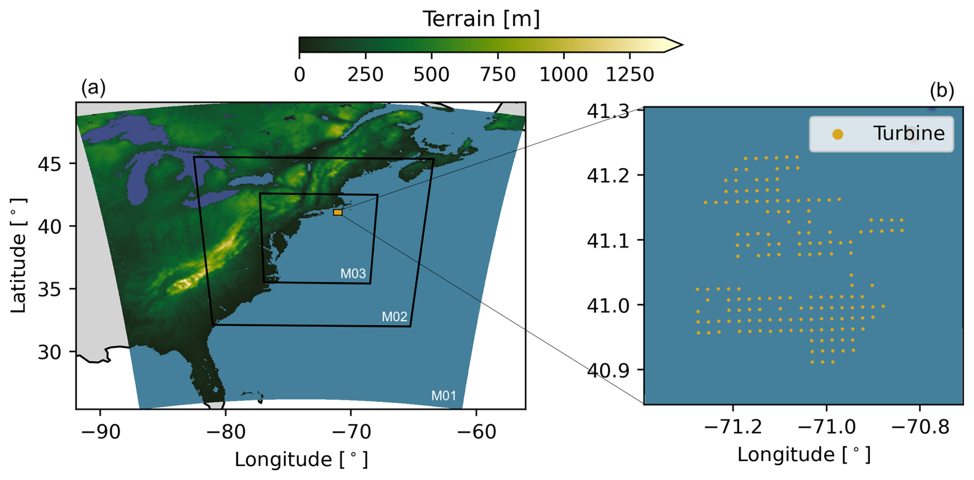
Figure 1 Domain layout for the mesoscale (a) and LES (b) domains. The location of the turbines within the LES domain is also shown.

The LES and mesoscale simulations employ similar physics parameterizations to ensure a direct comparison between both modeling frameworks. Water vapor, cloud water, rain, cloud ice, snow, and graupel processes are represented using the Thompson microphysics scheme (Thompson et al., 2008). Longwave and shortwave radiation effects are included in the simulations via the Rapid Radiative Transfer Model for Global Climate Models (RRTMG; Iacono et al., 2008). The Noah land surface model (Chen and Dudhia, 2001) and Monin–Obukhov similarity theory (Dyer and Hicks, 1970) are used to provide moisture, heat, and momentum fluxes at the bottom boundary of the domains. Unresolved convection in the outer mesoscale domain (i.e., domain M01) is modeled using the Kain–Fritsch scheme (Kain, 2004). Due to the grid spacing of the mesoscale simulations (Δx≥1 km), turbulence mixing must be parameterized. Here, we use the Mellor–Yamada–Nakanishi–Niino (MYNN) Level 2.5 boundary layer parameterization (Nakanishi and Niino, 2006) for all mesoscale domains. For the LES, we use the nonlinear backscatter and anisotropy model with turbulence kinetic energy (TKE)-based stress terms to represent subgrid-scale turbulence (Kosović, 1997; Mirocha et al., 2010).

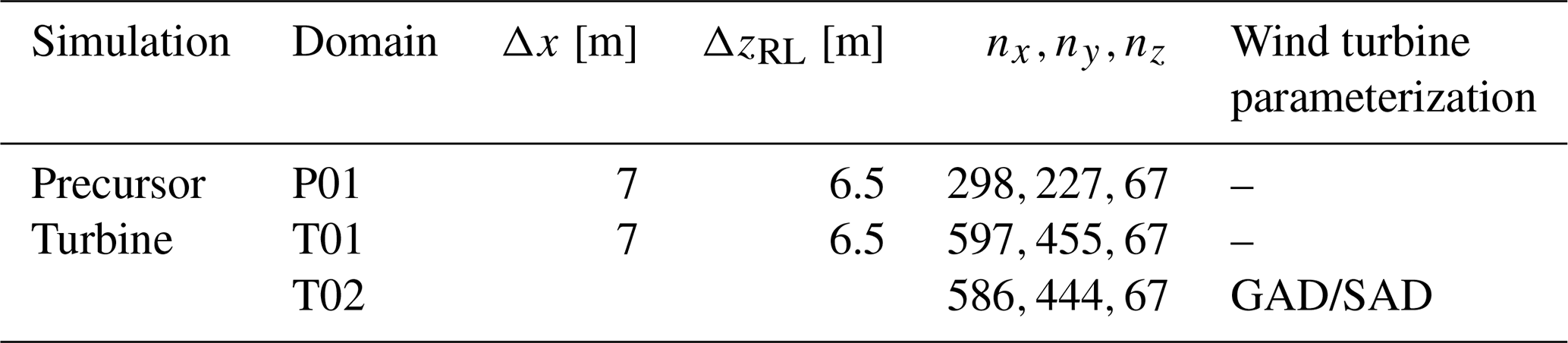
Table 1 Domain setup for the mesoscale and large-eddy simulations, including the horizontal grid spacing Δx, the mean vertical spacing across the turbine rotor layer Δz_RL, the number of grid points along each direction n_i, the choice of wind turbine parameterization in each domain, and turbulence closure.

MYNN: Mellor–Yamada–Nakanishi–Niino, WFP: wind farm parameterization, NBA: nonlinear backscatter and anisotropy.

2.1 Wind turbine positions

Wind farms located in the Massachusetts and Rhode Island lease areas are subject to additional environmental and technical constraints that influence turbine spacing (e.g., BOEM, 2021). As a result, their layouts typically follow uniform east–west and north–south grid patterns with 1  nm×1  nm spacing (1  nm≈1.852  km), consistent with US Coast Guard recommendations (USCG, DHS, 2020). South Fork Wind, Revolution Wind, and Sunrise Wind are expected to install 11  MW turbines based on turbine supplier agreements (McCoy et al., 2024). We populate the lease areas using publicly available data from each project's construction and operation plan (Jacobs Engineering Group Inc., 2021; Vanasse Hangen Brustlin, Inc., 2023; Stantec Consulting Services Inc., 2021), assuming a uniform 1.852  km×1.852  km spacing and 11  MW turbine rating, based on information available as of 13 March 2024.

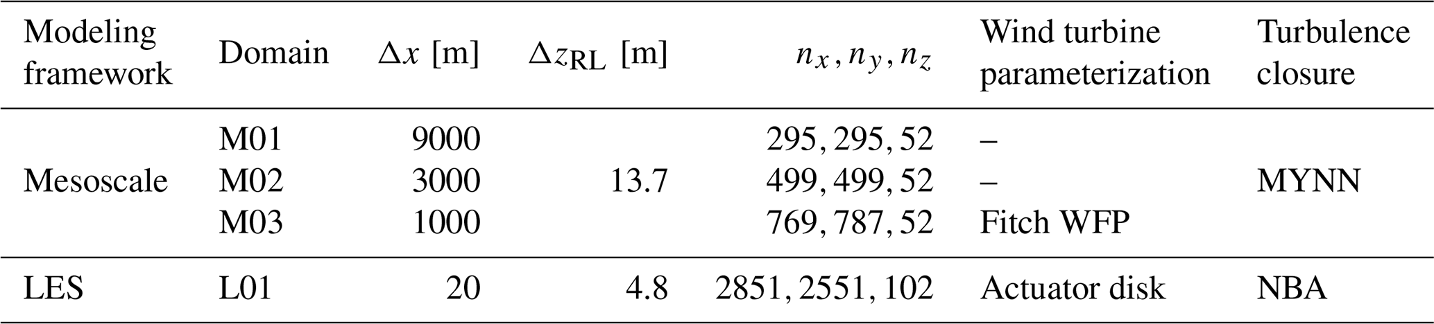
The three simulated wind farms consist of a total of 161 wind turbines with an average effective turbine spacing of about 4.8  km (23D) for wind directions between 200 and 250°. The turbine layout for the three simulated wind farms is shown in Fig. 2a. Under southwesterly flow – the predominant wind direction in the region (Musial et al., 2013; Bodini et al., 2019; Rosencrans et al., 2024) – the directions of alignment within a 7  km radius for each turbine are 205, 212, 224, 235, and 243° (Fig. 2b) with average spacing of 4.1  km (20D), 6.7  km (33D), 2.7  km (13D), 6.7  km (33D), and 4.1  km (20D), respectively. Due to the domain discretization and because the turbines are represented at the grid cell center, the simulated turbine positions in the mesoscale simulation differ from their physical location (Fig. 2). On average, the simulated turbine positions in the mesoscale simulation are displaced by 400 m (∼2D) from their physical position, with a maximum displacement of 700 m (∼3.4D). As a result, the effective turbine positions in the mesoscale simulation also have slightly different directions of alignment compared to the LES (Fig. 2b, d). New directions of alignment are also evident, as illustrated by the dashed black line in Fig. 2d. Moreover, in some cases, turbines within the wind farm can be separated by a single grid cell (i.e., 1  km) rather than the physical 1.852  km spacing. Subsequent analysis is based on the turbine spacing and directions of alignment defined by the physical turbine positions.

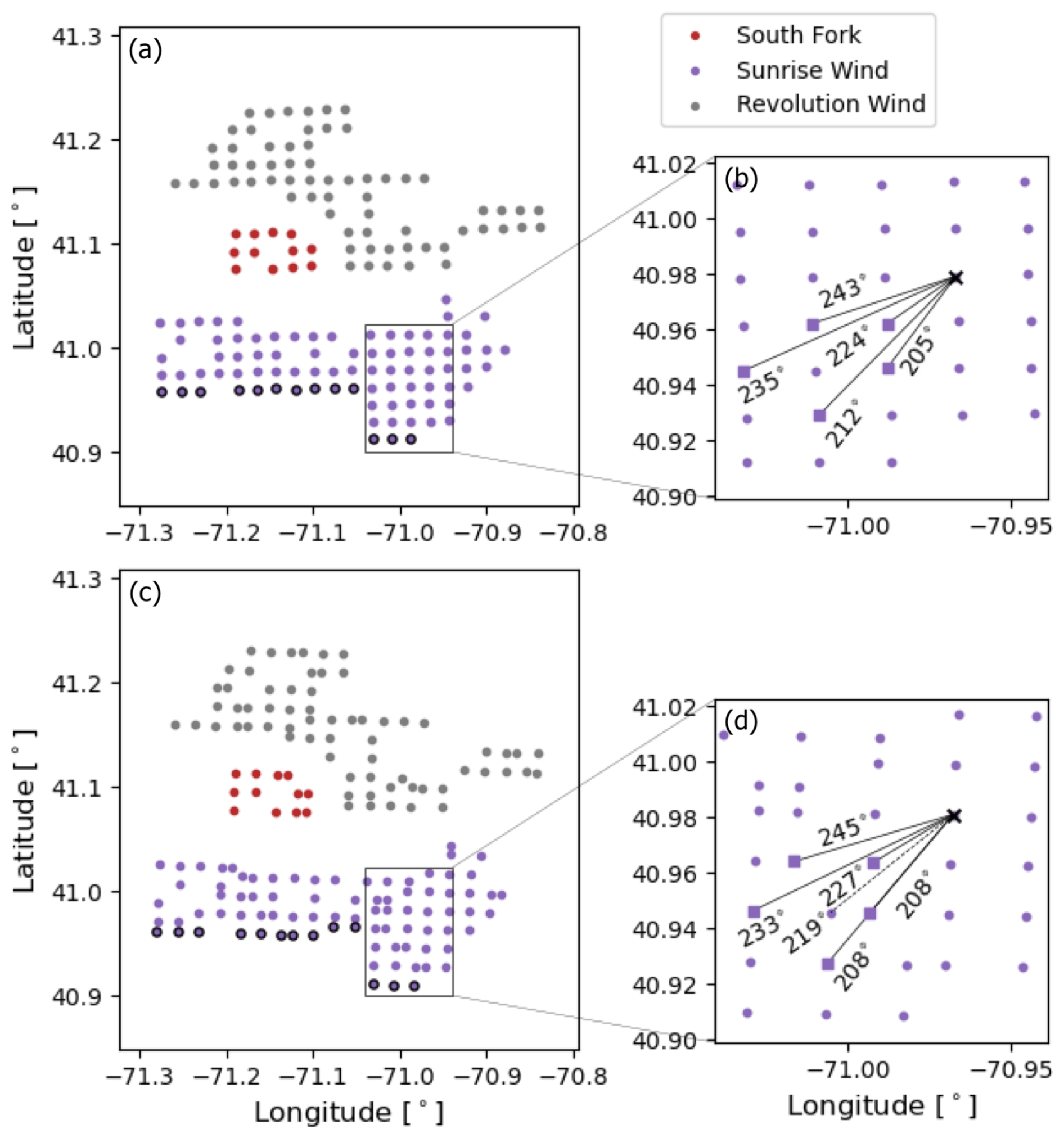
Figure 2 Wind farm layout for the South Fork (red), Sunrise Wind (purple), and Revolution Wind (grey) wind farms. Panel (a) shows the physical turbine positions, while panel (c) shows the turbine layout in the mesoscale simulation. Front-row turbines for southwesterly flow are highlighted with black circles in panels (a) and (c). Panels (b) and (d) illustrate the directions of alignment measured clockwise from true north for turbines in Sunrise Wind within a 7  km radius under southwesterly flow. Note that the effective directions of alignment change in the mesoscale simulation due to the domain discretization. An additional direction of alignment in the mesoscale simulation is represented by the dashed line in panel (d).

3 Atmospheric conditions

We investigate wake effects for a range of atmospheric conditions representative of the region under consideration. Winds on the US East Coast are predominantly from the southwest (Musial et al., 2013; Bodini et al., 2019; Rosencrans et al., 2024); therefore, we search for dates when the wind direction at hub height is around ϕ=225°. To study internal wake effects, we also select cases when the wind direction creates an aligned wind farm arrangement (i.e., 205, 225, 240°). Based on these criteria, our analysis considers a narrow wind sector within [202.5, 247.5°]. Hub-height wind speeds below rated speed (11  m s⁻¹) are chosen so that the wake-induced velocity deficit translates entirely into power reduction. Finally, although we consider atmospheric stability conditions that range from weakly stable to weakly unstable, we focus our analysis on weakly stable conditions, as these can have a substantially higher impact on downstream wind turbines.

Table 2 Summary of atmospheric conditions for the five simulated cases, including mean hub-height wind speed ${\stackrel{\mathrm{‾}}{U}}_{\mathrm{h}}$ and direction ${\stackrel{\mathrm{‾}}{\mathit{\varphi }}}_{\mathrm{h}}$ and the minimum and maximum values of $z/L$ and Ri_B throughout the simulation time.

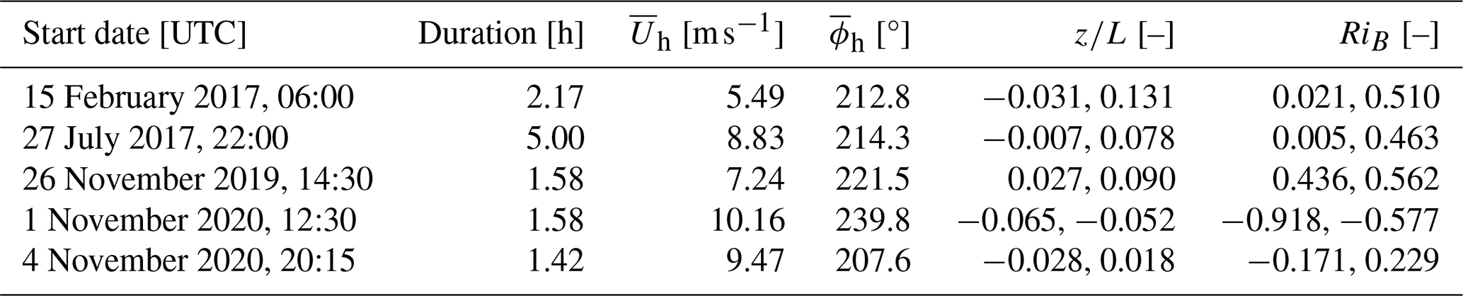
To this end, we perform LESs and mesoscale simulations of five dates that match the desired wind speed, wind direction, and stability criteria. Table 2 summarizes the atmospheric conditions for each of the simulated cases. We characterize atmospheric stability at the surface and across the turbine rotor layer using data at the wind farms' locations using the finest-resolution mesoscale domain (M03) without turbines. Stability at the surface is defined here using the inverse of the Obukhov length normalized by height (Eq. 1), where u_* is the friction velocity, θ_s is the surface temperature, κ=0.4 is the von Kármán constant, g is the gravitational acceleration, ${\dot{Q}}_{\mathrm{s}}$ is the surface kinematic heat flux, and z=10  m. Here, we define stable conditions as $z/L>\mathrm{0}$ and unstable conditions as $z/L\le \mathrm{0}$. Because atmospheric stability across the turbine rotor layer may differ from that at the surface (Rosencrans et al., 2024; Xia et al., 2025), we also quantify stability across the turbine rotor layer using the bulk Richardson number (Eq. 2), where the vertical gradients of potential temperature (θ) and wind speed (u,v) are estimated between the surface (z=10  m) and the top of the turbine rotor layer (z=236  m). Here, we define stable conditions as Ri_B>0 and unstable conditions as Ri_B≤0.

$$\begin{array}{}\text{(1)}& {\displaystyle }z/L={\displaystyle \frac{z\mathit{\kappa }g{\dot{Q}}_{\mathrm{s}}}{-u_{*}^{\mathrm{3}}{\mathit{\theta }}_{\mathrm{s}}}}\text{(2)}& {\displaystyle }{\mathit{Ri}}_B={\displaystyle \frac{(g/\stackrel{\mathrm{‾}}{\mathit{\theta }})\mathrm{\Delta }\stackrel{\mathrm{‾}}{\mathit{\theta }}\mathrm{\Delta }z}{(\mathrm{\Delta }\stackrel{\mathrm{‾}}{u}{)}^{\mathrm{2}}+(\mathrm{\Delta }\stackrel{\mathrm{‾}}{v}{)}^{\mathrm{2}}}}\end{array}$$

The simulated cases cover a range of variability in wind speeds, wind directions, and temperature profiles throughout the lower portion of the boundary layer (Fig. 3). 15 February 2017 is characterized by a near-constant wind speed across the rotor layer with a large (almost 35°) southerly shift in wind direction over time. Atmospheric stability at the surface and across the rotor layer is initially weakly unstable and evolves to be weakly stable. 27 July 2017 exhibits a shallow boundary layer with slow changes in wind speed and direction over time. Both the surface and the rotor layer stability transition from near-neutral conditions to weakly stable conditions. The boundary layer on 26 November 2019 remains weakly stable throughout the simulated times and shows a steady increase in wind speed as the wind shifts toward the west. On 1 November 2020, wind speed at turbine heights remains nearly constant over time, while the wind direction shifts toward the south. Atmospheric stability remains unstable at turbine heights and at the surface. Finally, 4 November 2020 exemplifies a transition from an unstable boundary layer to a near-neutral surface layer, while stability across the rotor layer becomes weakly stable. Wind speed varies slightly over time, while the wind shifts in direction toward more westerly flow.

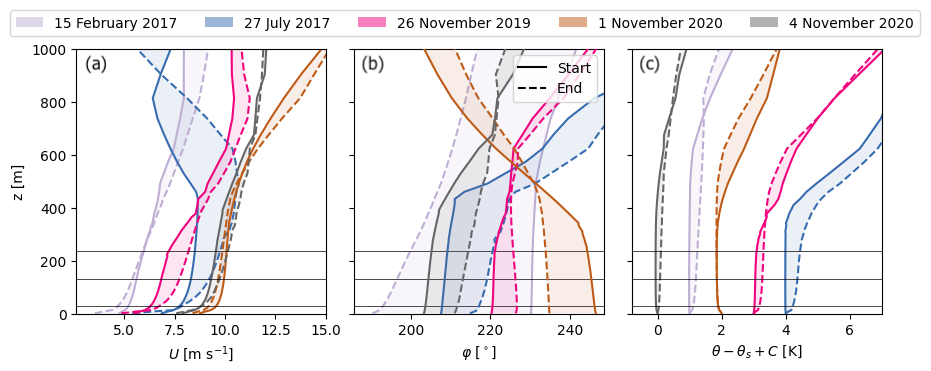
Figure 3 Vertical profiles of wind speed (a), wind direction (b), and potential temperature (c) for the five simulated dates. For each date, the first and last valid time stamps are represented by the solid and dashed lines, respectively, while time stamps in between are represented by the filled colors. The horizontal black lines in each panel represent the bottom of the rotor, hub height, and top of the rotor for the 11  MW wind turbine.

Wind conditions throughout the five simulated cases enable analysis of internal and cluster wake effects for a variety of atmospheric stability conditions. To evaluate the representativeness of our simulations, we compare the simulated atmospheric conditions with long-term (20-year) data from the National Offshore Wind dataset (NOW-23; Bodini et al., 2020, 2024). Hub-height wind speed for the selected cases is consistently below rated speed (Fig. 4a) so that the largest wake effects occur (Lundquist et al., 2019). The hub-height wind direction is ϕ_h=217°, on average, and includes the directions of alignment for the turbines in the wind farms (i.e., 205, 225, 240°) (Fig. 4b). Furthermore, the most common wind direction in the simulated cases is between 215 and 220°, matching the most frequent wind direction according to the climatology of the region. Surface layer and rotor layer stability is predominantly stable for the selected cases (Fig. 5). Most of the simulated cases (75 %) exhibit stable conditions across the turbine rotor layer, whereas 25 % of cases exhibit unstable conditions at turbine heights (Fig. 5b). The long-term climatology also shows that a majority of cases are stable (79 %) rather than unstable (21 %) based on the Richardson number. Similarly, 68 % of the cases are stable and 32 % are unstable based on the surface stability criteria (Fig. 5a), which is comparable to the surface layer stability estimates from the climatology of the region (57 % stable and 43 % unstable). Note that these simulations are not designed to evaluate wake effects across atmospheric conditions that are fully representative of the climatology of this region; rather, the purpose is to capture typical conditions and examine how the mesoscale modeling framework performs.

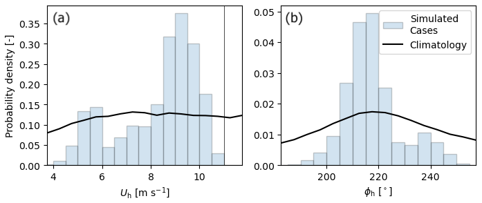
Figure 4 Probability density distribution for wind speed (a) and wind direction (b) at hub height (133  m) in the highest-resolution mesoscale domain (M03) for a simulation without turbines. The velocity field at hub height is sampled spatially across the region covered by the wind farms and temporally every 5 min. The black lines illustrate the climatology of the region based on the 2023 National Offshore Wind dataset (NOW-23; Bodini et al., 2020, 2024). The wind speed and wind direction distributions from NOW-23 are sampled at z=140  m. The wind speed distribution from NOW-23 is shown for wind directions between 180 and 270°.

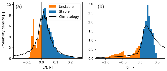
Figure 5 Probability density for the atmospheric stability at the surface (a) and across the turbine rotor layer (b) in the highest-resolution mesoscale domain (M03) for a simulation without turbines. The stability metrics are sampled spatially across the region covered by the wind farms and temporally every 5 min. The black lines illustrate the climatology of the region based on the 2023 National Offshore Wind dataset (NOW-23; Bodini et al., 2020, 2024). The stability metrics from NOW-23 are shown for wind directions between 180 and 270°.

4 Velocity deficit

The velocity fields at hub height (z=133  m) are averaged in time to provide an adequate comparison between the LES and the mesoscale solution. The horizontal wind speed fields are averaged using 15 min time windows, corresponding to 15 time stamps from the LES and 3 time stamps for the mesoscale simulation. Figure 6 illustrates the time-averaged wind speed at hub height for the mesoscale simulation and LES on 4 November 2020 at 20:37 UTC.

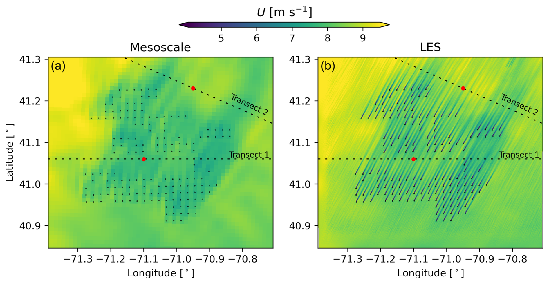
Figure 6 Time-averaged velocity field at hub height for the mesoscale simulation (a) and LES (b) on 4 November 2020 at 20:37 UTC. The dotted black lines in each panel illustrate the locations of the velocity transects, and the red dots indicate the midpoint distance of each transect.

We compare the time-averaged velocity from the LES and mesoscale simulation at two different locations to examine the ability of the mesoscale model to represent cluster wakes. We consider the velocity field immediately upstream of South Fork and Revolution Wind to investigate the combined wake of all turbines in Sunrise Wind (transect 1 in Fig. 6). We sample the velocity field approximately 2Δx_meso (Δx_meso=1  km) south of the leading turbines in South Fork and Revolution Wind to avoid mesoscale winds at turbine-containing grid points, which is equivalent to approximately 5.2  km, or 25.2 rotor diameters (25.2D), north of Sunrise Wind. We also consider the velocity field downstream of the three wind farms to investigate the combined wake of all turbines in the domain (transect 2 in Fig. 6). Transect 2 is approximately perpendicular to the mean wind direction for the simulated cases and is about 7.4  km (36D) downstream of Revolution Wind. The location of Transect 2 is selected to capture the full spatial extent of the wake under the wind directions analyzed here.

The transects of the time-averaged velocity field from the LES are averaged spatially to provide a more direct comparison with the mesoscale wind fields. A 1  km moving average is applied to the LES velocity transects to filter out flow features smaller than the grid spacing of the mesoscale domain. Spatial averaging effectively removes small-scale features of the flow that cannot be captured by the mesoscale grid while retaining the signal from individual turbine wakes that sometimes persist far downstream.

Differences in the wake between the LES and mesoscale simulation are evaluated using the root-mean-square error (RMSE). The RMSE between the LES and mesoscale simulation for each 15 min time window t is calculated following Eq. (3), where ${\stackrel{\mathrm{‾}}{U}}_{\mathrm{LES}}(t,x$) is the time- and space-averaged velocity transect of the LES, ${\stackrel{\mathrm{‾}}{U}}_{\mathrm{meso}}(t,x$) is the time-averaged transect of the mesoscale simulation, x_i is the distance along each transect 𝒯 defined in Fig. 6, and N is the number of grid points along each transect. Note that the velocity transect for the mesoscale simulation is interpolated to match the spatial resolution of the LES. We also calculate the RMSE of the normalized velocity difference between the LES and mesoscale simulation ($\widehat{\mathrm{RMSE}}$) to account for larger differences at faster wind speeds (Eq. 4).

$$\begin{array}{}\text{(3)}& {\displaystyle }\mathrm{RMSE}\left(t\right)=\sqrt{\sum _{x_i\in \mathcal{T}}{\displaystyle \frac{{\left({\stackrel{\mathrm{‾}}{U}}_{\mathrm{meso}}(t,x_i)-{\stackrel{\mathrm{‾}}{U}}_{\mathrm{LES}}(t,x_i)\right)}^{\mathrm{2}}}{N}}}\text{(4)}& {\displaystyle }\widehat{\mathrm{RMSE}}\left(t\right)=\sqrt{\sum _{x_i\in \mathcal{T}}{\displaystyle \frac{{\left({\stackrel{\mathrm{‾}}{U}}_{\mathrm{meso}}(t,x_i)-{\stackrel{\mathrm{‾}}{U}}_{\mathrm{LES}}(t,x_i)\right)}^{\mathrm{2}}}{{\stackrel{\mathrm{‾}}{U}}_{\mathrm{LES}}^{\mathrm{2}}(t,x_i)N}}}\end{array}$$

4.1 Cluster wake between wind farms

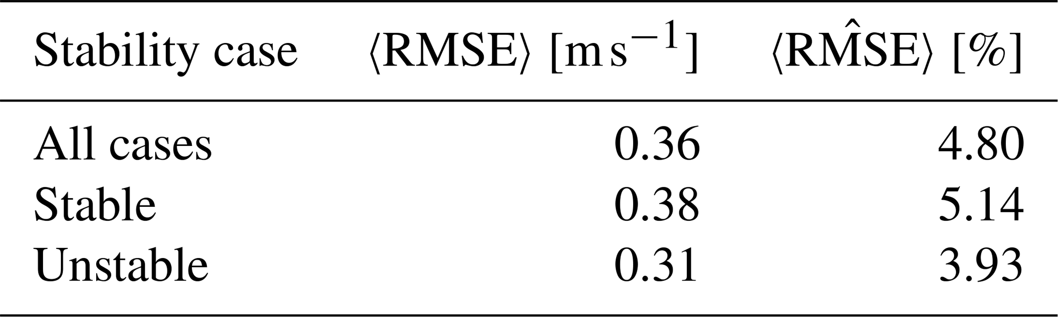
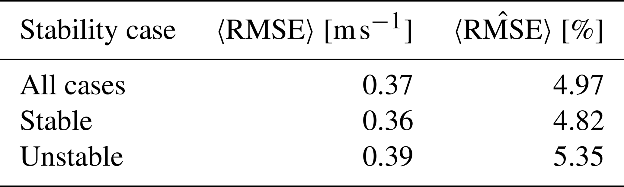
The combined wake of the turbines in Sunrise Wind is well captured by the mesoscale simulation, especially under unstable atmospheric conditions (Table 3). The average RMSE of the velocity field in the wake of Sunrise Wind between the LES and mesoscale simulation is about 0.3  m s⁻¹ across the different stability cases. On average, the RMSE between the LES and mesoscale simulation is 10 % larger in the stable case than in the unstable case. The RMSE of the normalized velocity differences ($\widehat{\mathrm{RMSE}}$) further illustrates the larger discrepancies between the two modeling approaches. Although the difference in RMSE between the LES and mesoscale simulation for unstable and stable conditions is small (0.07  m s⁻¹), the normalized RMSE under stable conditions is 1 percentage point larger than under unstable conditions. The $\widehat{\mathrm{RMSE}}$ is larger in the stable case because individual turbine wakes may persist far downstream (increasing the magnitude of ${\stackrel{\mathrm{‾}}{U}}_{\mathrm{meso}}-{\stackrel{\mathrm{‾}}{U}}_{\mathrm{LES}}$ in the numerator of Eq. 4) and because the wake recovers faster under unstable conditions (increasing the magnitude of the denominator ${\stackrel{\mathrm{‾}}{U}}_{\mathrm{LES}}^{\mathrm{2}}$ in Eq. 4).

Table 3 Mean root-mean-square error (RMSE) between the LES and mesoscale simulation for each stability case. The RMSE is calculated for the velocity immediately upstream of the Revolution Wind and South Fork wind farms (transect 1 in Fig. 6).

Under stable conditions, the individual wakes of the turbines in Sunrise Wind can persist far downstream and reach the front-row turbines of the downstream clusters. Figure 7 exemplifies some of the limitations of the mesoscale simulation in capturing near-range cluster wakes. The individual turbine wakes are apparent in the time- and space-averaged LES velocity field (Fig. 7b, c), especially downstream of the northeast turbines of Sunrise Wind. In contrast, in the mesoscale simulation, the effects of individual turbine wakes do not persist far downstream (Fig. 7a, c). Furthermore, when the wind direction is aligned with the turbines, the wakes from the aligned turbines in Sunrise Wind combine and form a distinct and large velocity deceleration that may not be well captured by the mesoscale solution (Fig. 7c). As shown in Sect. 5.2, a mesoscale simulation cannot resolve individual turbine wakes, especially when the wind direction matches the direction of alignment for the turbines inside the wind farm.

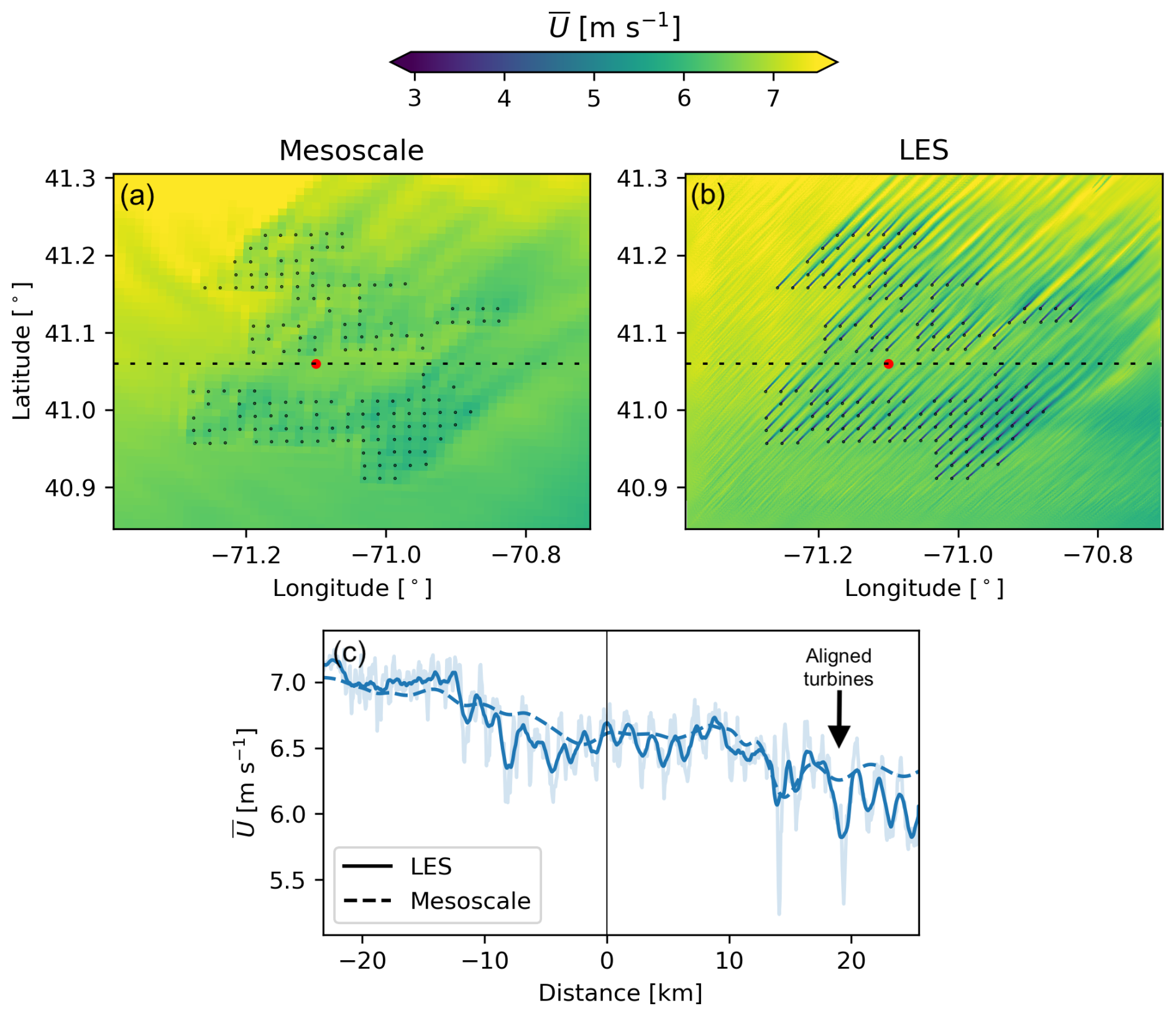
Figure 7 Time-averaged velocity field at hub height for the mesoscale simulation (a) and LES (b) under stable atmospheric conditions. The velocity fields are averaged in time between 14:30 and 14:45 UTC on 26 November 2019. The dotted black lines in each panel illustrate the locations of the velocity transects, and the red dots indicate the midpoint distance of each transect. Panel (c) shows the velocity along the transect for the LES and mesoscale simulation. For reference, the mean wind direction across the region is 219°.

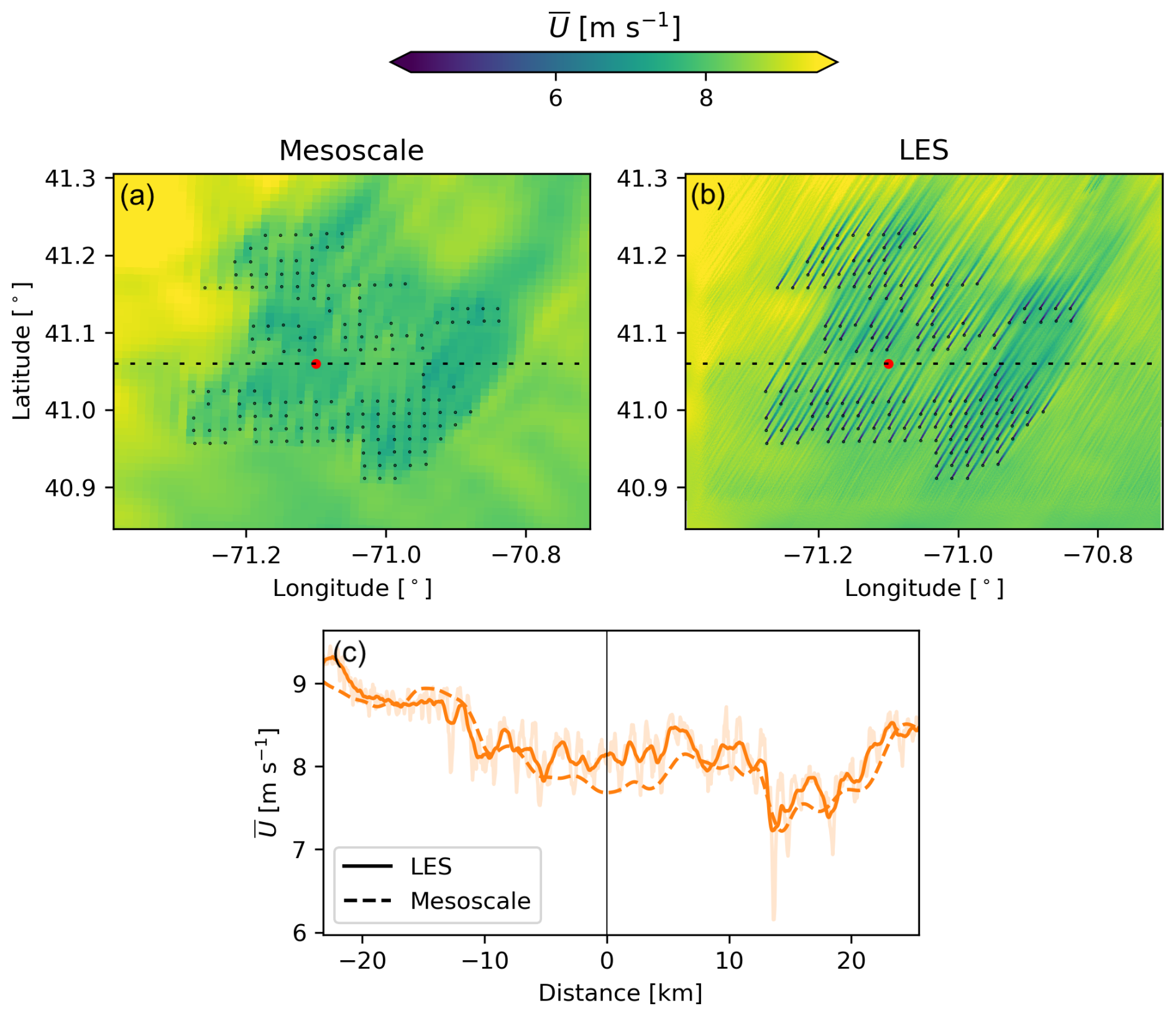
Figure 8 Time-averaged velocity field at hub height for the mesoscale simulation (a) and LES (b) under unstable atmospheric conditions. The velocity fields are averaged in time between 22:00 and 22:15 UTC on 27 July 2017. The dotted black lines in each panel illustrate the locations of the velocity transects, and the red dots indicate the midpoint distance of each transect. Panel (c) shows the velocity along the transect for the LES and mesoscale simulation. For reference, the mean wind direction across the region is 208°.

Under unstable stability conditions, individual turbine wakes generally merge with the larger-scale cluster wake before reaching downstream clusters (Fig. 8). As a result, the difference between the wake in the LES and mesoscale simulation is smaller. This faster wake recovery under unstable conditions is driven by enhanced turbulent mixing associated with larger turbulent stresses. In the mesoscale simulations, these effects are represented implicitly through increases in TKE and stability-dependent mixing length scales within the boundary layer parameterization (Nakanishi and Niino, 2009). Conversely, the LES explicitly resolves the dominant turbulent eddies responsible for enhanced mixing, providing a more direct representation of these effects. Even though individual turbine wakes may not persist far downstream, larger localized velocity decelerations still occur, like downstream of the northeast turbines in Sunrise Wind. The mesoscale simulations can accurately capture these localized velocity decelerations in the flow in unstable conditions.

4.2 Combined cluster wake from all wind farms

The combined cluster wake of the three wind farms is well captured by the mesoscale simulations for both stability cases (Table 4). Both the RMSE and the $\widehat{\mathrm{RMSE}}$ between the LES and mesoscale simulation are comparable for stable and unstable conditions. In contrast to the results in Sect. 4.1, the difference between the LES and mesoscale simulation is slightly larger for unstable conditions, as wake recovery is underestimated in the coarser grid. Nevertheless, the combined wake from all the turbines in the domain is well represented in the mesoscale simulations.

Table 4 Mean root-mean-square error (RMSE) between the LES and mesoscale simulation for each stability case. The RMSE is calculated for the velocity downstream of the three wind farms (transect 2 in Fig. 6).

The combined wake of the three wind farms under stable conditions is characterized by a distinct broad wind speed deficit. Figure 9 illustrates the typical wake under stable conditions. Individual turbine wakes are evident in the LES wind fields but not in the mesoscale ones, especially in the northern portion of the domain, where turbines in Revolution Wind do not experience the cluster wake from South Fork or Sunrise Wind. Moreover, because the mesoscale simulation cannot resolve individual turbine wakes, it also cannot capture the velocity acceleration in between the individual wakes. To compensate, the winds accelerate on the lateral sides of the wind farm faster in the mesoscale simulation. It is likely that a similar but opposite phenomenon occurs upstream of the wind farm, where the wind decelerates due to blockage. Nevertheless, the mesoscale simulation accurately represents the magnitude of the larger-scale deceleration downstream of the three wind farms and the spatial gradient in the wake. To illustrate, the pronounced velocity deceleration in the northeast part of the domain, driven by the combined wake effects from the high turbine concentration in the northeastern region of Sunrise Wind and the eastern turbines of Revolution Wind, is well captured (red arrow in Fig. 9c).

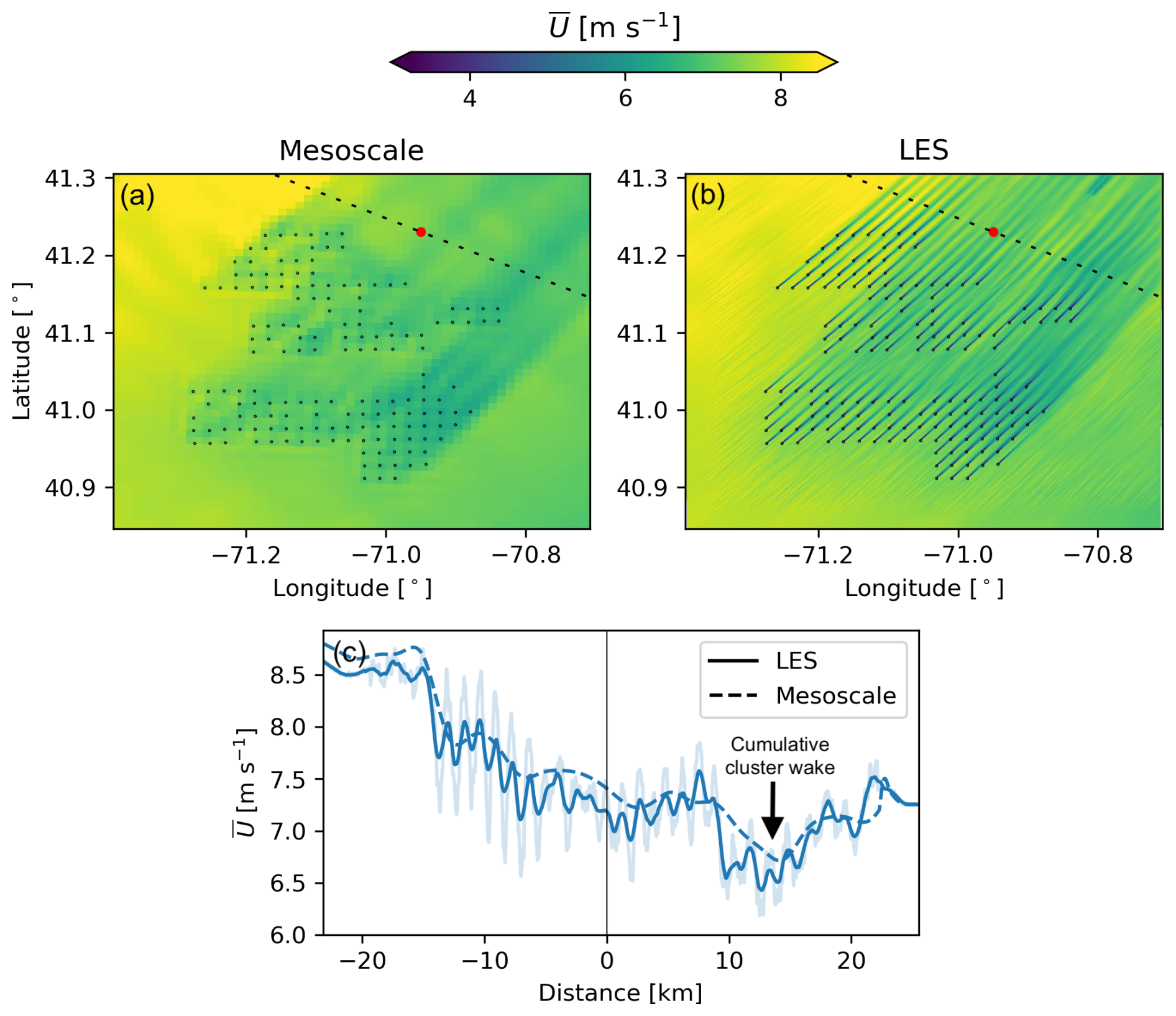
Figure 9 Time-averaged velocity field at hub height for the mesoscale simulation (a) and LES (b) under stable atmospheric conditions. The velocity fields are averaged in time between 15:45 and 16:00 UTC on 26 November 2019. The dotted black lines in each panel illustrate the locations of the velocity transects, and the red dots indicate the midpoint distance of each transect. Panel (c) shows the velocity along the transect for the LES and mesoscale simulation. For reference, the mean wind direction across the region is 223°.

Under unstable conditions, the combined wake of the three wind farms exhibits a bimodal shape. Figure 10 illustrates the typical wake under unstable conditions. Just as individual turbine wakes recover more quickly under unstable atmospheric conditions, the collective wake of the wind farms also recovers faster than in stable conditions. The bimodal structure of the combined cluster wake arises from the rapid recovery in the central portion of the wake (Fig. 10c), which is accurately captured by the mesoscale simulation. In contrast to the stable cases, individual turbine wakes are not evident downstream of the three wind farms (Fig. 10c).

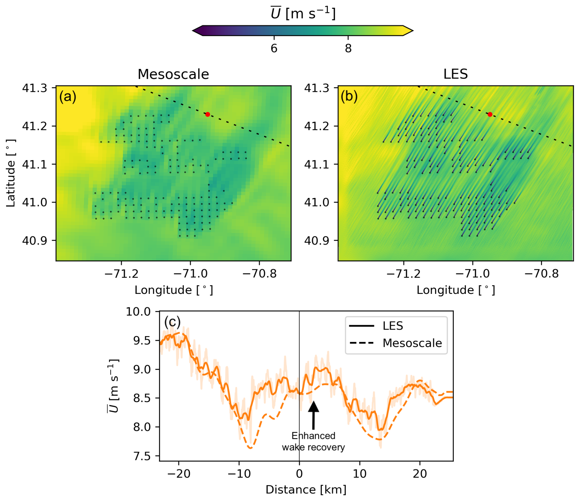
Figure 10 Time-averaged velocity field at hub height for the mesoscale simulation (a) and LES (b) under unstable atmospheric conditions. The velocity fields are averaged in time between 22:00 and 22:15 UTC on 27 July 2017. The dotted black lines in each panel illustrate the locations of the velocity transects, and the red dots indicate the midpoint distance of each transect. Panel (c) shows the velocity along the transect for the LES and mesoscale simulation. For reference, the mean wind direction across the region is 208°.

5 Wind turbine power

To compare the power production of the turbines in the LES and mesoscale simulation, we apply a 10 min moving average to the power data in the LES to remove fluctuations in power production caused by turbulence in the flow. Furthermore, we normalize the time-averaged power production of each turbine in the domain. The normalized power production of the ith turbine in the domain (${\widehat{P}}_i$) is defined as the ratio between the time-averaged power (${\stackrel{\mathrm{‾}}{P}}_i$) and the mean power of the front-row turbines in Sunrise Wind $\langle {\stackrel{\mathrm{‾}}{P}}_j\left(t\right){\rangle }_{j\in \mathrm{FR}}$ for southwesterly flow (illustrated as black circles in Fig. 2). In this way, we evaluate the ability of the mesoscale model to capture changes in power production relative to freestream conditions for a variety of wind speeds.

$$\begin{array}{}\text{(5)}& {\widehat{P}}_i\left(t\right)={\displaystyle \frac{{\stackrel{\mathrm{‾}}{P}}_i\left(t\right)}{\langle {\stackrel{\mathrm{‾}}{P}}_j\left(t\right){\rangle }_{j\in \mathrm{FR}}}}\end{array}$$

We compare the normalized power between the LES and the mesoscale simulation for turbines that are subject to internal wakes and turbines that only experience wakes from an upstream cluster. A turbine is considered to be subject to internal wakes when it has an immediate upstream neighbor under southwesterly flow (ϕ_h≈225°). Because the turbines in each wind farm are separated by 1.852  km (9D), any turbine with an upstream neighbor within 3  km (14.5D) will be subject to internal wakes (red circles in Fig. 11). Because some turbines in South Fork and Revolution Wind will experience a combination of internal and external wakes, we only consider turbines in Sunrise Wind for the internal wake analysis. To examine cluster wakes, we consider the turbines in South Fork and Revolution Wind that are only expected to be impacted by the wake from Sunrise Wind (blue circles in Fig. 11).

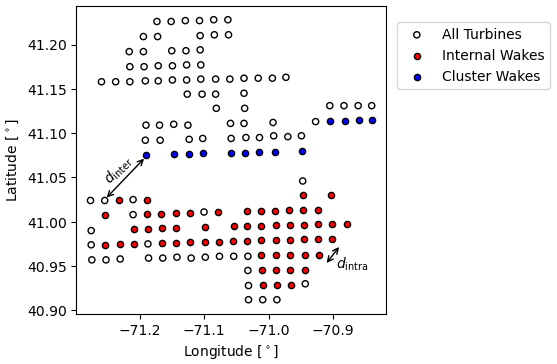
Figure 11 Wind turbine positions for the three wind farms. Turbines considered for the internal wake analysis are shown as red circles. Turbines considered for the cluster wake analysis are shown as blue circles. The distance between aligned turbines within the wind farm (d_intra) and the distance between clusters (d_inter) are also shown.

The mesoscale simulation shows more skill in capturing the effect of short-range cluster wakes than that of internal wakes within a wind farm (Fig. 12). Although the mesoscale simulation can accurately capture the velocity deceleration from the entire Sunrise Wind cluster (Sect. 4.1), the normalized power production of the front-row turbines in Revolution Wind and South Fork is not necessarily well represented (Fig. 12a). The slope of the regression line of the LES and mesoscale simulation data is only 0.55, and the regression coefficient is R²=0.5 for cluster-waked turbines. Nevertheless, the median normalized power across all wind direction sectors is $\widehat{P}=\mathrm{0.893}$ and $\widehat{P}=\mathrm{0.895}$ for the LES and mesoscale simulation, respectively. This behavior shows that, although the mesoscale simulation is not capable of capturing the mean variability in turbine power, it may be capable of representing the average cluster wake effect on downstream turbines when considering a broad range of wind direction sectors, albeit perhaps due to compensating errors. The mesoscale simulation struggles even more in capturing the mean variability in turbine power inside the wind farms (Fig. 12b). Both the slope of the regression line and the regression coefficient are smaller for internal wakes than for cluster wake effects. The mesoscale simulations generally underestimate internal wake effects within the wind farms compared to the LES for the same wind directions. The median normalized power of internally waked turbines is $\widehat{P}=\mathrm{0.87}$ in the LES, whereas it is $\widehat{P}=\mathrm{0.84}$ in the mesoscale simulations.

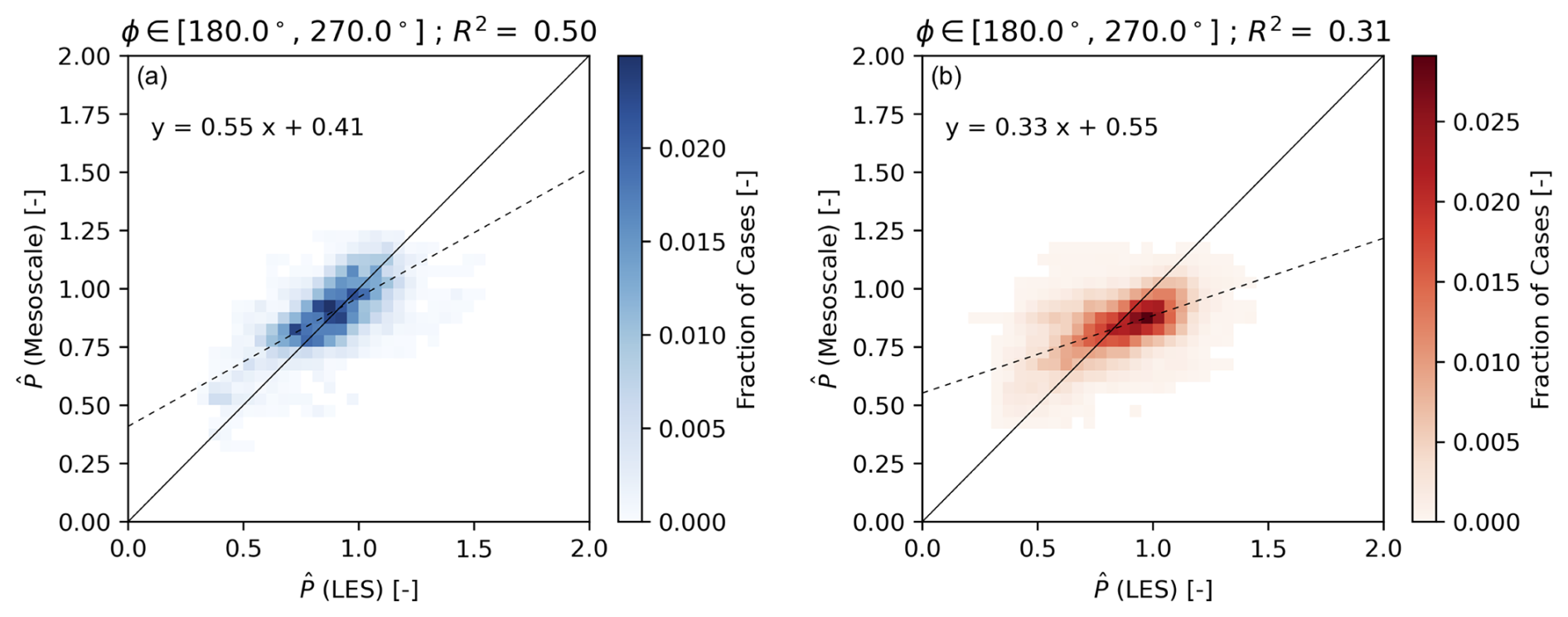
Figure 12 Normalized power production for turbines experiencing cluster wakes (a) and internal wakes (b) across all the wind direction sectors. The solid black line in each panel represents the 1:1 correspondence between the data. The dashed black line corresponds to the linear regression to the data, given in the top-left corner of each panel.

To provide additional insight into the strengths and limitations of mesoscale simulations, we now segregate the normalized power production based on the time-averaged wind direction at the location of each turbine. The mean distance (d_inter) between the last-row turbines in Sunrise Wind and the southernmost turbines in South Fork and Revolution Wind (Fig. 11) varies with wind direction. The effective spacings between the trailing turbines in Sunrise Wind and the leading turbines in the downstream wind farms are, on average, 9.5  km (46D), 10.9  km (53D), 12.4  km (60D), 14.8  km (72D), and 21.2  km (103D) for the wind direction sectors $\mathrm{200}\mathit{°}\le \mathit{\varphi }<\mathrm{210}\mathit{°}$, $\mathrm{210}\mathit{°}\le \mathit{\varphi }<\mathrm{220}\mathit{°}$, $\mathrm{220}\mathit{°}\le \mathit{\varphi }<\mathrm{230}\mathit{°}$, $\mathrm{230}\mathit{°}\le \mathit{\varphi }<\mathrm{240}\mathit{°}$, and $\mathrm{240}\mathit{°}\le \mathit{\varphi }<\mathrm{250}\mathit{°}$, respectively. The average spacing of turbines inside the wind farms (d_intra) also varies with wind direction (Fig. 11). Turbines are closest to their upstream neighbor ($d_{\mathrm{intra}}=\mathrm{2.7}\mathrm{km}\approx \mathrm{13}D$) when the wind direction is within $\mathrm{220}\mathit{°}\le \mathit{\varphi }<\mathrm{230}\mathit{°}$. The effective turbine spacing increases to $d_{\mathrm{intra}}=\mathrm{4.1}\mathrm{km}\approx \mathrm{20}D$ for wind direction sectors $\mathrm{200}\mathit{°}\le \mathit{\varphi }<\mathrm{210}\mathit{°}$ and $\mathrm{240}\mathit{°}\le \mathit{\varphi }<\mathrm{250}\mathit{°}$. The farthest effective spacing occurs for $\mathrm{210}\mathit{°}\le \mathit{\varphi }<\mathrm{220}\mathit{°}$ and $\mathrm{230}\mathit{°}\le \mathit{\varphi }<\mathrm{240}\mathit{°}$, with $d_{\mathrm{intra}}=\mathrm{6.7}\mathrm{km}\approx \mathrm{33}D$.

5.1 Cluster wake effects

Mesoscale simulations are better able to capture cluster wake effects for wind direction sectors where aligned turbines are spaced far apart from each other (Fig. 13). The slope of the regression line between the LES and mesoscale simulation increases and approaches 1.0 as the effective distance in between arrays d_inter increases (Fig. 13a–d). Furthermore, the difference between the average normalized power in the LES and mesoscale simulations remains within 2 percentage points for wind directions within $\mathrm{210}\mathit{°}\le \mathit{\varphi }<\mathrm{240}\mathit{°}$. The effective spacing between the turbines in Sunrise Wind and the leading turbine of South Fork and Revolution Wind exceeds d_inter>50D (d_inter⪆10  km) when the wind direction is between $\mathrm{210}\mathit{°}\le \mathit{\varphi }<\mathrm{240}\mathit{°}$; therefore, the individual turbine wakes of Sunrise Wind have generally already merged with the larger-scale wind farm wake before reaching the downstream clusters.

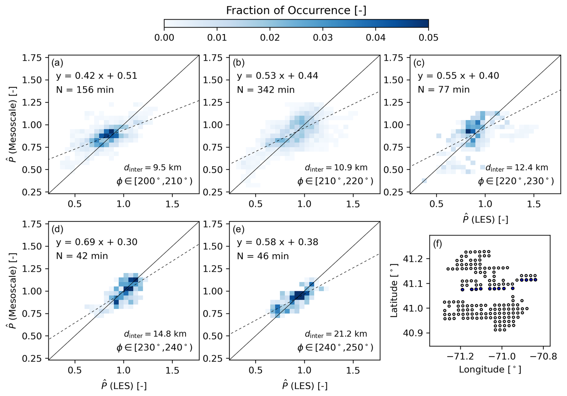
Figure 13 Normalized power production for turbines experiencing cluster wakes for wind direction sectors $\mathrm{200}\mathit{°}\le \mathit{\varphi }<\mathrm{210}\mathit{°}$ (a), $\mathrm{210}\mathit{°}\le \mathit{\varphi }<\mathrm{220}\mathit{°}$ (b), $\mathrm{220}\mathit{°}\le \mathit{\varphi }<\mathrm{230}\mathit{°}$ (c), $\mathrm{230}\mathit{°}\le \mathit{\varphi }<\mathrm{240}\mathit{°}$ (d), and $\mathrm{240}\mathit{°}\le \mathit{\varphi }<\mathrm{250}\mathit{°}$ (e). The turbines considered here are represented by the blue circles in panel (f). The solid black line in panels (a)–(e) represents the 1:1 correspondence between the data, and the dashed black line corresponds to the linear regression to the data, given in the top-left corner of each panel. The effective distance between the last-row turbines in Sunrise Wind and the southernmost turbines in South Fork and Revolution Wind (d_inter) is also shown in each panel.

The mesoscale simulation struggles to represent the effect of cluster wakes when the effective distance between the arrays is small. The mesoscale simulation greatly underestimates variability in turbine power compared to the LES when the wind direction is between $\mathrm{200}\mathit{°}\le \mathit{\varphi }<\mathrm{210}\mathit{°}$ (Fig. 13a). The slope of the regression line in the data is only 0.42. Moreover, the difference between the average normalized power in the LES and mesoscale simulations remains the largest for this wind direction sector (4 percentage points). Because the effective distance between aligned turbines is the smallest for $\mathrm{200}\mathit{°}\le \mathit{\varphi }<\mathrm{210}\mathit{°}$, individual turbine wakes from Sunrise Wind can impact the leading turbines in downstream clusters. Moreover, 72 % of the simulated cases for this wind direction sector correspond to stable conditions. As shown in Sect. 4.1, individual turbine wakes can persist far downstream in stable conditions and reach the downstream cluster. Because the mesoscale simulation cannot resolve individual turbine wakes, it also cannot capture the variability in turbine power production that is primarily caused by individual wakes.

The mesoscale simulation also struggles to represent cluster wake effects when the wind direction has a strong westerly component. As the wind direction shifts toward westerly flow ($\mathit{\varphi }\in [\mathrm{240}\mathit{°},\mathrm{250}\mathit{°})$), the effective distance between the trailing turbines in Sunrise Wind and the front-row turbines in Revolution Wind and South Fork becomes large; as a result, the cluster wake from Sunrise Wind is well represented in the mesoscale simulation. However, the front-row turbines in Revolution Wind and South Fork incorrectly wake each other in the mesoscale simulation for ϕ>240°. Due to the grid spacing of the mesoscale simulation and the numerical discretization of the model, front-row turbines in Revolution Wind and South Fork (red dots in Fig. 14a) wake their neighbors. In the LES, individual turbine wakes are clearly resolved, and the front-row turbines in Revolution Wind and South Fork do not wake each other (Fig. 14b). Consequently, the slope of the regression line decreases compared to $\mathrm{230}\mathit{°}\le \mathit{\varphi }<\mathrm{240}\mathit{°}$ (Fig. 13d, e). Interestingly, the average normalized power remains similar between the LES and mesoscale simulations ($\widehat{P}=\mathrm{0.91}$ and $\widehat{P}=\mathrm{0.92}$, respectively). This agreement arises because, in the mesoscale simulations, front-row turbines at Sunrise Wind wake their neighbors for wind directions between $\mathrm{230}\mathit{°}\le \mathit{\varphi }<\mathrm{240}\mathit{°}$. As a result, both the numerator and the denominator in Eq. (5) are reduced such that the relative power difference between freestream and cluster-waked turbines remains comparable across both approaches.

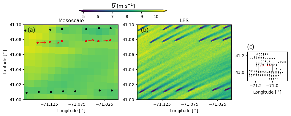
Figure 14 Time-averaged velocity field at hub height for the mesoscale simulation (a) and LES (b) on 1 November 2020 at 12:52 UTC. The mean wind direction at hub height is 245°. Panel (c) shows the region considered in panels (a) and (b). Front-row turbines in South Fork and Revolution Wind waking their neighbors are highlighted with the red circles in panels (a) and (c).

5.2 Internal wake effects

Internal wake effects are generally not well captured by the mesoscale simulations for the wind direction sectors considered here (Fig. 15). In general, the agreement between the LES and mesoscale simulations increases as the effective turbine spacing d_intra becomes larger. As the effective turbine spacing increases, the impact of the mesoscale discretization (i.e., error in turbine position and alignment offset) likely diminishes due to the wake expansion. Internal wake effects are highly underestimated when the effective turbine spacing is about 2.7  km (13D) (Fig. 15c) and the wind direction is aligned with the turbine layout. Conversely, internal wake effects may be better represented when the effective turbine spacing exceeds 30D (d_intra=6.7  km) (Fig. 15b, d).

Mesoscale simulations have limited skill in representing the variability in turbine power caused by internal wake effects for closely spaced turbines (Fig. 15a, c, e). Changes in mean turbine power are generally not well captured by the mesoscale simulation, indicated by the slope of the regression lines remaining smaller than 0.45 for $d_{\mathrm{intra}}<\mathrm{5}\mathrm{km}\approx \mathrm{24}D$. The LES shows large power reductions for $\mathrm{220}\mathit{°}\le \mathit{\varphi }<\mathrm{230}\mathit{°}$, as internally waked turbines generate, on average, 37 % less power than freestream turbines. The mesoscale simulations also show a reduction in turbine power; however, turbines inside the wind farm only generate 16 % less power, on average, than front-row turbines in Sunrise Wind. Figure 16b illustrates that while turbines in the LES are being directly waked by their upstream neighbors, turbines in the mesoscale simulation experience a weaker wake because the numerical grid cannot resolve individual wakes (Fig. 16a). Moreover, due to the numerical discretization of the model, the velocity reduction at each turbine grid cell propagates to the downstream turbine via the neighboring grid cells in Δx=1  km increments, wrongfully waking neighboring turbines that are not aligned with the local wind direction (Fig. 16a). This shows that turbines in adjacent grid cells will always be waked in some capacity by their neighbors. A similar effect occurs for $\mathrm{200}\mathit{°}\le \mathit{\varphi }<\mathrm{210}\mathit{°}$ and $\mathrm{240}\mathit{°}\le \mathit{\varphi }<\mathrm{250}\mathit{°}$, where the effective spacing is $d_{\mathrm{intra}}=\mathrm{4.1}\mathrm{km}\approx \mathrm{20}D$, but to a lesser degree. When the wind has a strong westerly component (ϕ≈245°), turbines inside the wind farm wake their neighbors in the mesoscale simulation but not in the LES. Therefore, the agreement between the LES and mesoscale simulation decreases for wind directions $\mathrm{240}\mathit{°}\le \mathit{\varphi }<\mathrm{250}\mathit{°}$ compared to $\mathrm{200}\mathit{°}\le \mathit{\varphi }<\mathrm{210}\mathit{°}$.

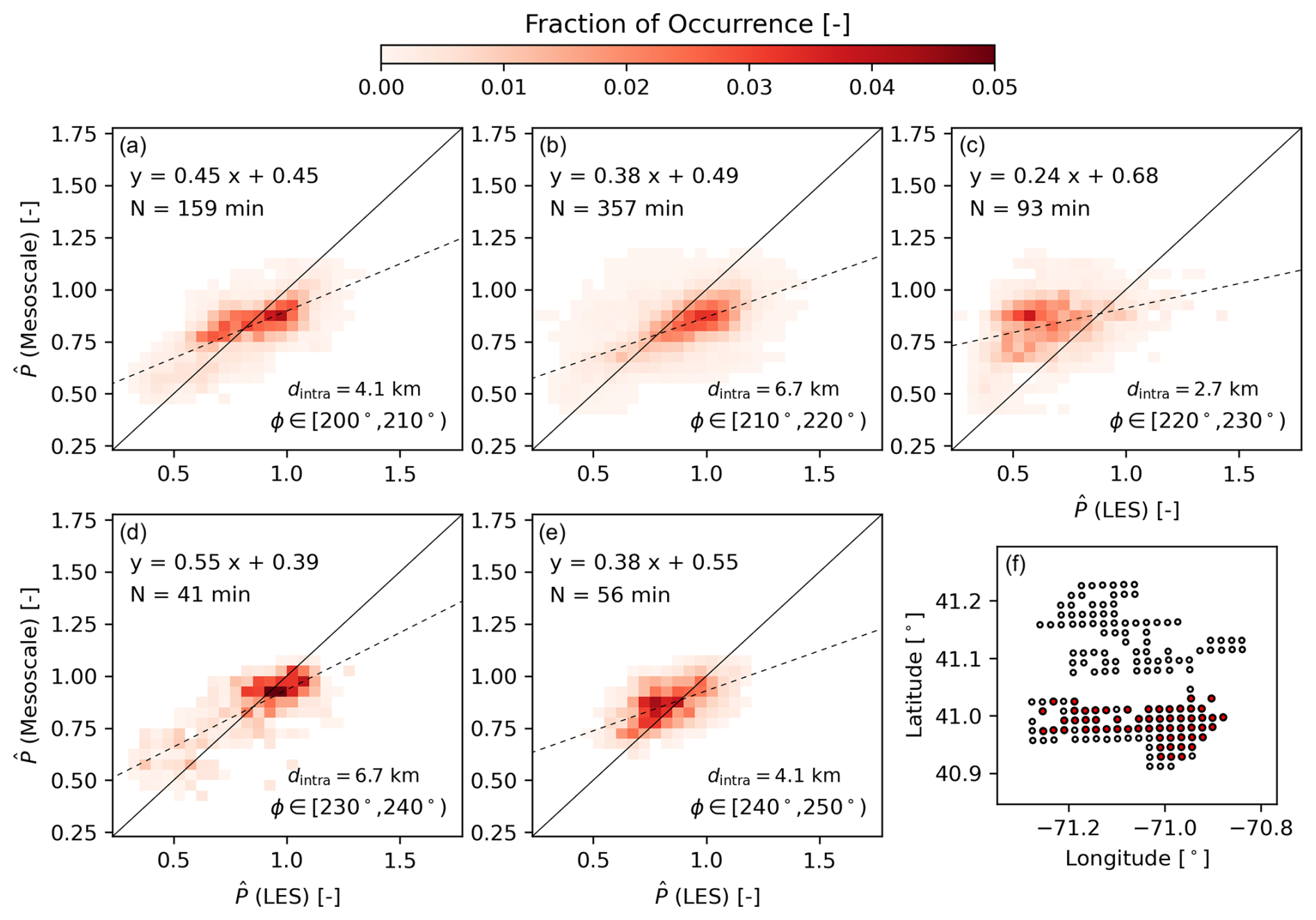
Figure 15 Normalized power production for turbines experiencing internal wakes for wind direction sectors $\mathrm{200}\mathit{°}\le \mathit{\varphi }<\mathrm{210}\mathit{°}$ (a), $\mathrm{210}\mathit{°}\le \mathit{\varphi }<\mathrm{220}\mathit{°}$ (b), $\mathrm{220}\mathit{°}\le \mathit{\varphi }<\mathrm{230}\mathit{°}$ (c), $\mathrm{230}\mathit{°}\le \mathit{\varphi }<\mathrm{240}\mathit{°}$ (d), and $\mathrm{240}\mathit{°}\le \mathit{\varphi }<\mathrm{250}\mathit{°}$ (e). Turbines considered here are represented by the red circles in panel (f). The solid black line in panels (a)–(e) represents the 1:1 correspondence between the data, and the dashed black line corresponds to the linear regression to the data, given in the top-left corner of each panel. The effective turbine spacing inside the wind farms (d_intra) is also shown in each panel.

Internal wake effects can be well captured when the effective turbine spacing is large and under unstable atmospheric conditions (Fig. 15b, d). The mesoscale simulation shows better agreement with the LES when $d_{\mathrm{intra}}=\mathrm{6.7}\mathrm{km}\approx \mathrm{33}D$ than when $d_{\mathrm{intra}}=\mathrm{4.1}\mathrm{km}\approx \mathrm{20}D$. As illustrated in Fig. 16d, the wake from an upstream turbine breaks down and merges with the wakes from the surrounding turbines; thus, individual turbine wakes are not as noticeable 6.7  km (33D) downstream. However, there is a distinct difference in agreement for $\mathrm{210}\mathit{°}\le \mathit{\varphi }<\mathrm{220}\mathit{°}$ and $\mathrm{230}\mathit{°}\le \mathit{\varphi }<\mathrm{240}\mathit{°}$. The mesoscale simulation generally overestimates internal wakes for $\mathrm{210}\mathit{°}\le \mathit{\varphi }<\mathrm{220}\mathit{°}$: internally waked turbines generate, on average, 16 % less power than freestream turbines in the mesoscale simulation compared to only 7 % less power in the LES. Differences between the mesoscale simulation and LES are smaller than 5 percentage points, on average, for $\mathrm{230}\mathit{°}\le \mathit{\varphi }<\mathrm{240}\mathit{°}$. Unstable conditions are prevalent for $\mathrm{230}\mathit{°}\le \mathit{\varphi }<\mathrm{240}\mathit{°}$; in contrast, there are more stable cases than unstable cases for the wind direction sector $\mathrm{210}\mathit{°}\le \mathit{\varphi }<\mathrm{220}\mathit{°}$. Because wakes recover faster under unstable conditions, the effect of internal wakes on downstream turbines is smaller, enabling better agreement between the mesoscale simulation and LES.

Figure 16 Time-averaged velocity field at hub height for the mesoscale simulation (a, c) and LES (b, d) on 26 November 2019 at 15:52 UTC (a, b) and 28 July 2017 at 00:07 UTC (c, d). The mean wind direction at hub height is 221° on 26 November 2019 at 15:52 UTC and 212° on 28 July 2017 at 00:07 UTC. Panel (e) illustrates the region shown in panels (a)–(d). The red arrows in panels (a) and (b) illustrate the predominant wake propagation direction in each modeling framework.

5.3 Combined cluster performance

After studying the ability of mesoscale simulations to capture the distinct effects of cluster or internal wakes, we now consider how each model compares when considering the power from the combined wind farm clusters. Just as for the individual turbine power, we normalize the combined power of all turbines at each time using the mean power of front-row turbines in Sunrise Wind. We also normalize the wind farm power using the total number of wind turbines in the domain (N_T). In this way, P_eq in Eq. (6) represents the average turbine performance across the three wind farms relative to the front-row turbines in Sunrise Wind. This metric provides an estimate of the cluster performance relative to freestream conditions. For example, if internal and cluster wake effects are negligible, then P_eq≈1.0, as most turbines will operate as if experiencing freestream. Conversely, if wake effects are large across most turbines, then P_eq≪1.0 because most turbines in the domain will experience slower winds than freestream.

$$\begin{array}{}\text{(6)}& {\widehat{P}}_{\mathrm{eq}}\left(t\right)={\displaystyle \frac{\sum {\stackrel{\mathrm{‾}}{P}}_i\left(t\right)}{N_{\mathrm{T}}\langle {\stackrel{\mathrm{‾}}{P}}_j\left(t\right){\rangle }_{j\in \mathrm{FR}}}}\end{array}$$

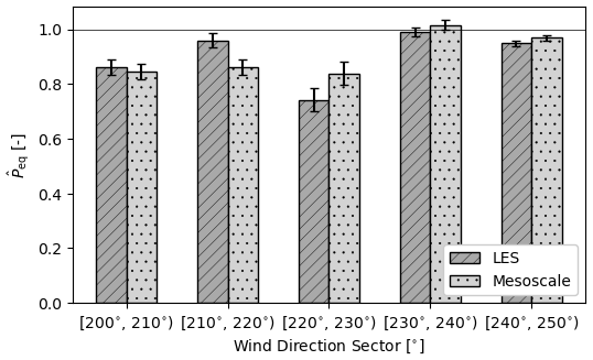
Figure 17 Normalized equivalent wind turbine power across the three wind farms for each wind direction sector for the mesoscale simulation and LES. The error bars represent the 95 % confidence interval in the data.

Although the mesoscale simulation may not accurately capture the variability in turbine power from internal wake effects, it may still provide an adequate estimate of the combined performance of the three wind farms for some wind direction sectors. The combined performance of the three wind farms is accurately represented in the mesoscale simulations for wind directions $\mathrm{200}\mathit{°}\le \mathit{\varphi }<\mathrm{210}\mathit{°}$ and $\mathrm{230}\mathit{°}\le \mathit{\varphi }<\mathrm{250}\mathit{°}$. The mesoscale simulations accurately represent the average performance of all wind turbines in the domain when internal and cluster wake effects are large (i.e., $\mathrm{200}\mathit{°}\le \mathit{\varphi }<\mathrm{210}\mathit{°}$) and when wake effects are small (i.e., $\mathrm{230}\mathit{°}\le \mathit{\varphi }<\mathrm{240}\mathit{°}$). However, the mesoscale simulation provides a statistically distinct estimate of combined cluster performance compared to the LES for $\mathrm{210}\mathit{°}\le \mathit{\varphi }<\mathrm{220}\mathit{°}$ and $\mathrm{220}\mathit{°}\le \mathit{\varphi }<\mathrm{230}\mathit{°}$. For $\mathrm{210}\mathit{°}\le \mathit{\varphi }<\mathrm{220}\mathit{°}$, the mesoscale simulation overestimates the combined internal and cluster wake effects across all turbines (${\widehat{P}}_{\mathrm{eq}}=\mathrm{0.96}$ for the LES and ${\widehat{P}}_{\mathrm{eq}}=\mathrm{0.86}$ for the mesoscale simulation). In contrast, the mesoscale simulation underestimates the combined wake effects across all turbines for $\mathrm{220}\mathit{°}\le \mathit{\varphi }<\mathrm{230}\mathit{°}$ (${\widehat{P}}_{\mathrm{eq}}=\mathrm{0.74}$ for the LES and ${\widehat{P}}_{\mathrm{eq}}=\mathrm{0.84}$ for the mesoscale simulation). Differences in combined cluster performance between the LES and mesoscale simulations stem primarily from the inability of the mesoscale simulation to accurately capture internal wake effects for these wind direction sectors.

6 Conclusions

This article presents a comprehensive case study highlighting the strengths and limitations of mesoscale simulations in capturing wake effects from wind turbine clusters and their impact on the power production of nearby turbine arrays. To this end, we provide a direct comparison of the data generated by mesoscale and LES modeling frameworks for three planned offshore wind farms on the US East Coast. The analysis considers realistic atmospheric conditions, including atmospheric stability for the most common wind directions and wind speeds in this region. To investigate the ability of mesoscale simulations to capture cluster wakes, we compare the velocity field from the mesoscale simulation and LES in the wake of a single wind turbine cluster and multiple wind turbine clusters. Because mesoscale simulations are increasingly being used to quantify wake effects in large wind farms, we also evaluate the variability in mean turbine power production in the mesoscale simulations and compare it with the LES results.

Mesoscale simulations are able to capture the velocity downstream of both a single wind turbine cluster and multiple offshore wind turbine clusters. The RMSE between the mesoscale simulation and LES is approximately 5 %, on average, downstream of a single wind farm and multiple wind farms. Moreover, the mesoscale simulation accurately captures stability-driven variations in wind farm wake behavior – for instance, narrower, faster-recovering wakes during unstable conditions and broader, longer-lasting wakes during stable conditions. Our findings concur with validation studies using field measurements (Siedersleben et al., 2018b; Cañadillas et al., 2022; Ali et al., 2023) and higher-fidelity models (Vanderwende et al., 2016; Fischereit et al., 2022b; García-Santiago et al., 2024), which found that mesoscale simulations adequately represent the velocity in the wake of wind turbine arrays. However, our results offer added value through a direct comparison between mesoscale simulation and LES frameworks under realistic atmospheric conditions.

Although the mesoscale simulations can represent the velocity in the wake of wind farms, they are a poor predictor of wake effects in the special circumstance when individual wakes persist over long distances and impact downstream turbines. Because individual turbine wakes typically influence only nearby downstream turbines within a wind farm, the mesoscale simulation highly underestimates changes in turbine power caused by internal wakes, especially when turbines become aligned with the predominant wind direction, as discussed in Radünz et al. (2025). Our findings agree with idealized simulations from Vanderwende et al. (2016), who showed that mesoscale simulations with grid spacing Δx≈1  km underestimate internal wake effects. It is possible that mesoscale simulations with finer grid spacing (Δx⪅1  km) can capture internal wake effects (Vanderwende et al., 2016); however, the assumptions made in boundary layer parameterizations do not hold with such grid spacing (Wyngaard, 2004; Rai et al., 2019), requiring parameterizations that can represent horizontal gradients of mean quantities (Juliano et al., 2022). Individual turbine wakes can also persist over long distances within the broader wind farm wake. Under these conditions, mesoscale simulations underestimate short-range cluster wake effects, as turbine power variations are driven more by localized velocity deficits from individual wakes than by the broader-scale flow deceleration of the full wind farm wake. Because mesoscale simulations do not resolve individual turbine wakes, they are better suited to capture short-range cluster and internal wake effects under unstable conditions, where wakes recover more rapidly, than under stable conditions, where wakes persist over longer distances. In addition, the discretization of turbine positions in the mesoscale grid introduces offsets from their physical locations that modify the effective directions of alignment and turbine spacing, contributing additional uncertainty to internal wake estimates. Mesoscale simulations are also more appropriate for representing long-range cluster wake effects, where individual wakes merge into the broader wind farm wake (Sanchez Gomez et al., 2024).

Although mesoscale simulations consistently underestimate changes in wind turbine power from internal and cluster wakes, they can still provide an accurate estimate of the combined power losses over some wind direction sectors. For the wind direction sectors considered here, the mesoscale simulations overestimate the combined cluster and internal wake impact for $\mathit{\varphi }\in [\mathrm{210}\mathit{°},\mathrm{220}\mathit{°})$ and underestimate losses for $\mathit{\varphi }\in [\mathrm{220}\mathit{°},\mathrm{230}\mathit{°})$. However, the mesoscale simulations accurately predict the combined internal and cluster wake losses across other wind direction sectors, even if the variability in turbine power caused by internal wakes is not well represented. Depending on the wind rose and the wind farm layout, it is possible for the internal wake under- and overestimations across wind direction sectors to balance out. For instance, if the wind direction sectors where wake losses are underestimated and overestimated are equally weighted and if the level of underestimation and overestimation is also comparable between both, then the mesoscale simulation may be an accurate predictor of the combined cluster and internal wake effect. However, it is likely that inaccuracies in the mesoscale simulation estimates will also change with the grid spacing, as larger grid spacing will change how neighboring turbines are wrongfully waked in the coarse grid.

A direct comparison of mesoscale simulations and LES of three offshore wind farms on the US East Coast highlights some of the limitations and strengths of mesoscale simulations in capturing wake effects. Although we show that the mesoscale simulations can accurately represent wind farm wake behavior, we find that they struggle to capture changes in energy output, especially from internal wake effects. This counterintuitive finding stems from the grid spacing and numerical discretization of the mesoscale framework, which limit the ability of mesoscale simulations to resolve internal wake dynamics (Radünz et al., 2025). Future work should directly quantify the contribution of turbine position errors in the mesoscale grid to the uncertainty in internal wake estimates, for example, by comparing simulations with physical and discretized turbine positions under otherwise identical conditions. The inability of mesoscale simulations to capture internal wake effects, which are typically larger than cluster wake effects, underscores the limitations of using such models to estimate wind farm energy output, especially for highly skewed wind roses. Although the findings from this study are derived from offshore simulations, the limitations from the mesoscale model also extend to onshore conditions because they are intrinsic to the model and not to the flow characteristics that distinguish onshore from offshore conditions. A limitation of our study is its representativeness across wind farm layouts and different mesoscale modeling frameworks. Different wind farm layouts will likely produce differences in the internal wake effects captured by the mesoscale simulation. Moreover, the choice of the mesoscale grid spacing (Vanderwende et al., 2016), boundary layer parameterization (Rybchuk et al., 2022), and wind farm parameterization options (Fischereit et al., 2022b) will also modify wake effects in the mesoscale model. Future studies should evaluate whether mesoscale simulations can represent the evolution of cluster wakes over longer distances (>50  km). In addition, a combination of mesoscale simulations and LES may be employed in future studies to consider the combined effect of long-range cluster wakes on downstream wind farms.

Appendix A: Spurious gravity waves

Spurious gravity waves can develop near the inflow domain boundaries of the LES and propagate inward. Spurious gravity waves develop as a result of the differences in vertical grid spacing between the LES and mesoscale simulations. The mesoscale simulation employs considerably coarser vertical grid spacing near the surface (Δz_meso=11  m) compared to the LES (Δz_LES=4  m). Similarly, the lowest vertical grid point is closer to the surface in the LES (z=2  m) than in the mesoscale simulation (z=6  m). Therefore, the horizontal wind speed near the surface that is provided as boundary conditions to the LES is extrapolated from a higher elevation, resulting in faster winds than would naturally develop close to the surface. Consequently, the horizontal wind speed near the surface decelerates as it enters the LES domain. The sudden deceleration of the horizontal wind near the surface triggers upward motions that generate spurious gravity waves in the capping inversion, which then propagate across the domain.

We include Rayleigh damping of the vertical velocity between the top of the boundary layer and the top of the LES domain (Eq. A1) to mitigate spurious gravity waves, following Khan et al. (2024). In Eq. (A1), d is the horizontal distance to the nearest lateral boundary, d_damp is the depth of the damping layer in the horizontal direction, z_bl is the boundary layer height defined by the capping inversion, w is the vertical velocity, γ is the damping coefficient, and $\mathit{\tau }={\sin }^{\mathrm{2}}\left[\frac{\mathit{\pi }}{\mathrm{2}}\left(\mathrm{1}-\frac{d}{d_{\mathrm{damp}}}\right)\left(\mathrm{1}-\frac{z_{\mathrm{top}}-z}{z_{\mathrm{top}}-z_{\mathrm{bl}}}\right)\right]$, where z_top≈21  km is the top of the domain. The damping distance is set to d_damp=10  km to encompass multiple wavelengths of spurious waves. The damping coefficient γ=5N is determined based on the height-averaged Brunt–Väisälä frequency N, and a factor of 5 is chosen to minimize reflections from the domain boundaries (Khan et al., 2024). Note that Rayleigh damping of the vertical velocity is performed only above the capping inversion to allow turbulence structures to develop naturally within the boundary layer.

$$\begin{array}{}\text{(A1)}& F_w=\left\{\begin{array}{lcl}-\mathit{\gamma }\mathit{\tau }(d,z)w& \text{if}& d\le d_{\mathrm{damp}}\text{and}z\ge z_{\mathrm{bl}}\\ \mathrm{0}& \text{if}& d>d_{\mathrm{damp}}\text{or}z<z_{\mathrm{bl}}\end{array}\right.\end{array}$$

Rayleigh damping near the lateral inflow boundaries of the LES effectively mitigates spurious gravity wave activity within the LES domain (Figs. A1 and A2). Spurious gravity waves can propagate throughout the LES domain and affect the velocity and temperature fields (Fig. A1a, c, e). These spurious waves extend throughout the entire boundary layer and above (Fig. A2a). By including Rayleigh damping in the lateral inflow boundaries of the LES, the velocity and temperature fields in the boundary layer and above no longer exhibit spurious gravity wave activity (Figs. A1b, d, f and A2b). Furthermore, turbulence structures can develop naturally within the boundary layer (Fig. A2b). Because these waves are nonphysical in nature, we include Rayleigh damping near the lateral boundaries in all LESs.

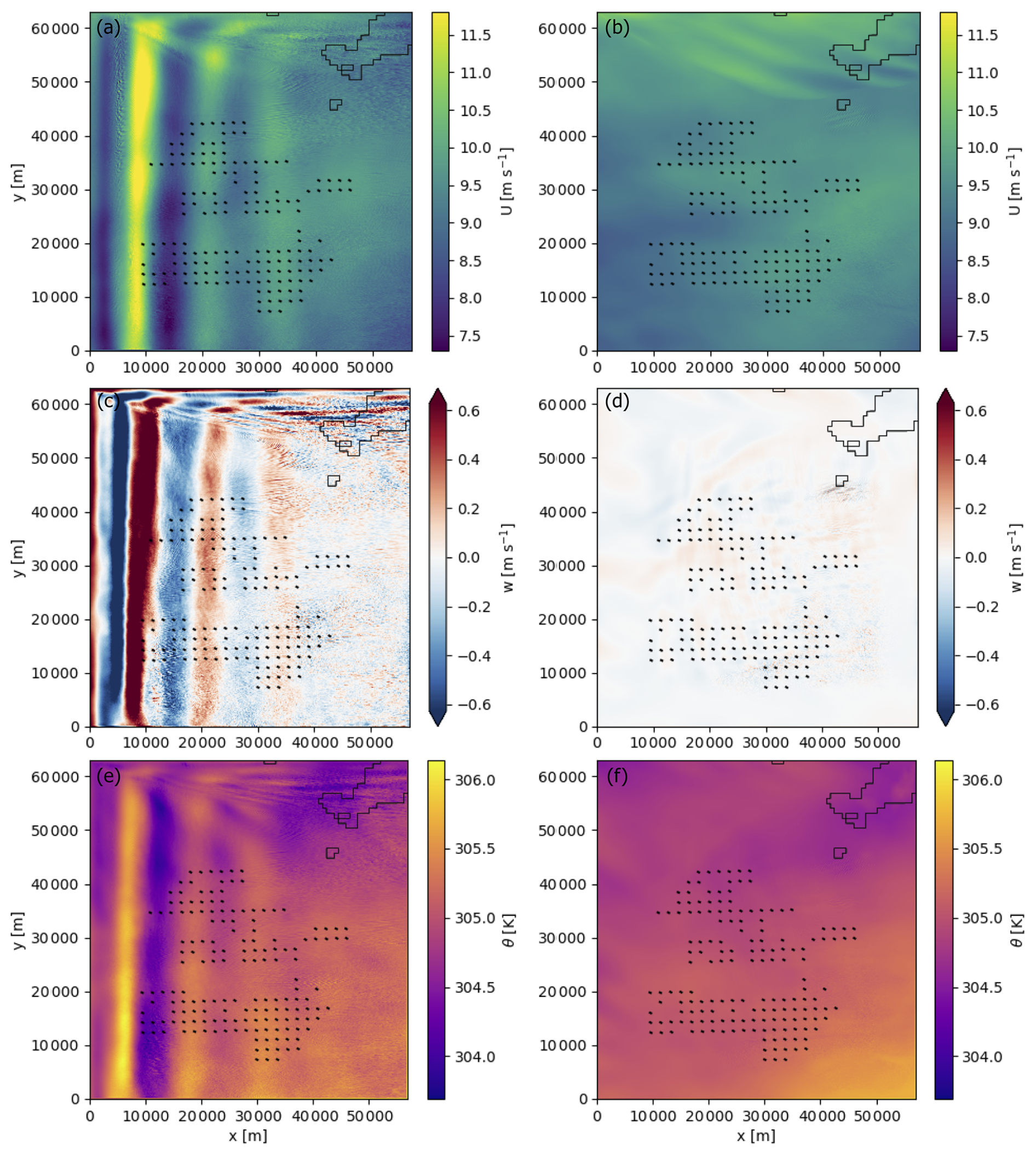
Figure A1 Plan view of the instantaneous horizontal wind speed (a, b), vertical wind speed (c, d), and potential temperature (e, f) fields at z=2  km for the LES without (a, c, e) and with (b, d, f) Rayleigh damping near the lateral inflow domain boundaries. The velocity fields are shown for 27 July 2017 at 22:00 UTC.

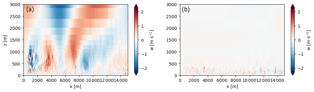
Figure A2 Vertical slice of the instantaneous vertical velocity field at y=30  km for the simulation without (a) and with (b) Rayleigh damping near the lateral inflow boundaries of the LES domain. The vertical velocity fields are shown for 27 July 2017 at 22:00 UTC.

Appendix B: Actuator disk model

An actuator disk model is implemented in WRF to represent the thrust of the wind turbines on the flow. The actuator disk model estimates the turbine's thrust and power production from the thrust (C_T) and the power (C_P) coefficient curves, respectively. The thrust dT and power dP of each differential element dA within the actuator disk are given by Eqs. (B1) and (B2), respectively, where ρ is the local air density, and U_∞ is the instantaneous wind speed 1D upstream of the wind turbine. The thrust and power coefficients are estimated as a function of the time-averaged hub-height wind speed 1D upstream of the turbine.

$$\begin{array}{}\text{(B1)}& {\displaystyle }\mathrm{d}T={\displaystyle \frac{\mathrm{1}}{\mathrm{2}}}\mathit{\rho }{U}_{\mathrm{\infty }}^{\mathrm{2}}{C}_{\mathrm{T}}\mathrm{d}A\text{(B2)}& {\displaystyle }\mathrm{d}P={\displaystyle \frac{\mathrm{1}}{\mathrm{2}}}\mathit{\rho }{U}_{\mathrm{\infty }}^{\mathrm{3}}{C}_{\mathrm{P}}\mathrm{d}A\end{array}$$

The numerical implementation of the actuator disk model presented here is based on the generalized actuator disk (GAD) model from Mirocha et al. (2014) and Aitken et al. (2014), but the forces of the flow and turbine power production are estimated using the thrust and power coefficient curves. To distinguish between both turbine parameterizations, we refer to the actuator disk model presented here as the simple actuator disk (SAD) model. The turbine's thrust is projected to the Cartesian grid following Eqs. (B3)–(B5), where Θ and Ψ are the turbine's yaw and tilt angles, respectively. The tilt angle is set to 4°, following Aitken et al. (2014). Furthermore, the forces are spread across multiple grid points using a Gaussian regularization kernel to ensure numerical stability. The SAD model provides more flexibility than the GAD model by only requiring the turbine's thrust and power coefficient curves. In contrast, the GAD model requires specifying the lift and drag curves for the airfoils at each radial location.

$$\begin{array}{}\text{(B3)}& {\displaystyle }\mathrm{d}{F}_x=\mathrm{d}T\cos \mathrm{\Theta }\cos \mathrm{\Psi }\text{(B4)}& {\displaystyle }\mathrm{d}{F}_y=\mathrm{d}T\sin \mathrm{\Theta }\cos \mathrm{\Psi }\text{(B5)}& {\displaystyle }\mathrm{d}{F}_z=-\mathrm{d}T\sin \mathrm{\Psi }\end{array}$$

We evaluate the wake evolution downstream of the SAD and GAD models using an idealized numerical framework (Table B1). An idealized weakly stable boundary layer develops in a small precursor domain with periodic boundary conditions (domain P01 in Table B1), following the $-\mathrm{0.2}\mathrm{K}{\mathrm{h}}^{-\mathrm{1}}$ case presented in Sanchez Gomez et al. (2023). Figure B1 illustrates the plane-averaged atmospheric conditions for the weakly stable boundary layer. The mean hub-height wind speed and direction are 8.3  m s⁻¹ and 269.6°, respectively. After turbulence is fully developed in the precursor simulation, we expand the numerical domain using the tiling strategy from Sanchez Gomez et al. (2023) to encompass a larger area. A two-domain one-way-nested setup is used to evaluate wake evolution downstream of the turbine (domains T01 and T02 in Table B1). The T01 domain employs periodic boundary conditions. We use the National Renewable Energy Laboratory (NREL) 5  MW reference wind turbine (Jonkman et al., 2009) to compare both turbine parameterizations, as both the airfoil characteristics required by the GAD and the thrust and power curves required by the SAD are publicly available. The NREL 5  MW wind turbine has a hub height of 90  m, a rotor diameter of 126  m, a cut-in speed at 3  m s⁻¹, a rated speed at 11  m s⁻¹, and a cut-out speed at 25  m s⁻¹. The turbine parameterization is only active in the T02 domain. We run the idealized simulations for 80 min, from which the first 10 min is discarded to allow the wake to propagate from the turbine location to the T02 domain outflow. The three-dimensional velocity fields and the turbine's thrust and power are saved every 30 s over the analysis period.

The SAD model accurately captures the power and thrust of the turbine over the simulated time period (Fig. B2). Just like the GAD model, the SAD model displays large variability in the power and thrust coefficients over the simulated time period. Nevertheless, the SAD model accurately represents the mean power and thrust of the turbine. The mean power and thrust coefficients are 0.44 and 1.00 for the SAD and 0.58 and 0.85 for the GAD, respectively. For a hub-height wind speed of 8.3  m s⁻¹, the power and thrust coefficients are expected to be 0.45 and 0.96, respectively. Therefore, the SAD model provides a more accurate representation of the turbine's thrust and power than the GAD model when compared to the turbine's reference curves.

Wake evolution downstream of the turbine is similar between the GAD and SAD models. In both cases, the wake meanders and erodes about 10D downstream of the turbine (Fig. B3). The mean wake evolution is also similar between both wind turbine parameterizations (Fig. B4). The time-averaged velocity fields show a strong deceleration in the near wake and slow recovery farther downstream (Fig. B4c). However, the wake deficit immediately downstream of the turbine is stronger in the SAD model, as the GAD model slightly underestimates the turbine's thrust compared to the reference curve (Fig. B2b). Nevertheless, the velocity deficit in the far wake is similar in both turbine parameterizations. Moreover, a region of flow acceleration develops between the bottom of the turbine rotor layer and the ground for the GAD and SAD models (Fig. B4a, b). Because the wake evolution far downstream of the turbine is comparable between the GAD and SAD models and because the SAD model accurately captures the thrust and power compared to the reference curves, the SAD model is considered adequate to investigate the cluster and internal wake effects on the US East Coast.

Table B1 Domain setup for the idealized LESs, including the horizontal grid spacing Δx, the mean vertical spacing across the turbine rotor layer Δz_RL, the number of grid points along each direction n_i, and the choice of wind turbine parameterization.

GAD: generalized actuator disk model, SAD: simple actuator disk model.

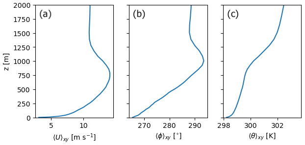
Figure B1 Space-averaged wind speed (a), wind direction (b), and potential temperature profile (c) for the idealized weakly stable boundary layer.

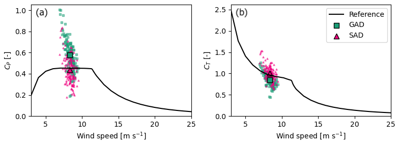
Figure B2 Power (a) and thrust (b) coefficient curves for the NREL 5  MW wind turbine. The instantaneous results are shown in green for the GAD and in magenta for the SAD. The large colored symbols with black edges in each panel represent the mean over the simulated time period.

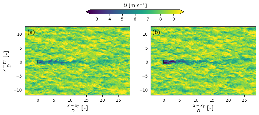
Figure B3 Instantaneous hub-height wind speed for the GAD (a) and SAD (b) wind turbine parameterizations. The location of the turbine is represented by the solid black line. The x and y axes are normalized to represent the distance in rotor diameters (D) from the turbine parameterization.

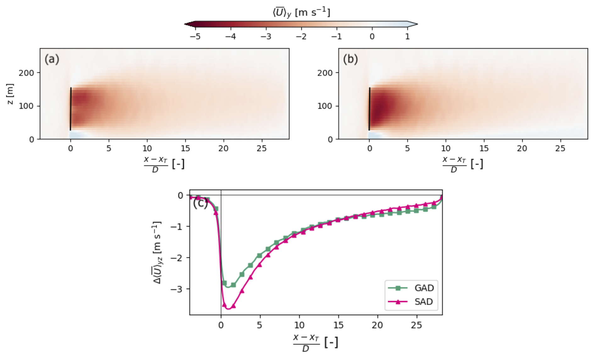
Figure B4 Time- and space-averaged wind speed deficit for the GAD (a) and SAD (b) wind turbine parameterizations at the turbine location. The rotor-averaged wind speed deficit is shown in panel (c). The velocity fields in panels (a) and (b) are averaged along the y direction across the turbine diameter. The rotor-averaged velocity field in panel (c) is also averaged vertically across the turbine rotor layer.