Graph neural operator for wind farm wake flow

Wind farm flow simulations are computationally expensive. However, numerous simulations are often required to account for wake effects from multiple neighboring farms, which motivates the development of data-driven surrogate models. Such surrogates may also enable the consideration of neighboring farm wakes during layout optimization.

Most existing data-driven surrogate approaches rely on fixed algebraic superposition principles, which may limit flexibility when extending to higher-fidelity data sources that capture nonlinear wake interactions. We propose a novel method that embeds a trainable and scalable superposition principle within a graph neural operator (GNO) architecture, enabling the model to learn complex wake combinations directly from data.

The model consists of two sequential graph neural network (GNN) layers: the first encodes turbine–turbine interactions into a latent representation, while the second combines these latent turbine states to predict the wind speed at a desired location. The GNO is trained on a large dataset generated with PyWake, a steady-state engineering wake model. More than 2000 unique layouts were procedurally generated for training, with an additional 998 for testing.

The GNO accurately identifies regions of strong wake interaction, although the spatial extent of wakes is slightly underestimated compared to the simulated values in cases with pronounced wake effects. Overall, the proposed GNO represents a methodological advancement in data-driven wind farm flow surrogates, introducing a new conceptual framework inspired by established engineering wake modeling principles.

1 Introduction

Wind farm flow has been studied rigorously since engineers placed multiple turbines together on farms. The phenomenon of wind-turbine-induced wakes is one of the most extensively studied subjects in wind energy; see, e.g., Göçmen et al. (2016); Porté-Agel et al. (2020). Nevertheless, accurately representing the complex interactions among multiple wakes remains an active research challenge. In classical engineering wind farm flow models, the total flow field is obtained by calculating the operating state of each turbine and determining its corresponding wake contribution. The combined wind farm flow is then found through wake superposition. This step forms the core of most engineering models and significantly contributes to their overall performance.

Traditionally, wake superposition is performed using simple algebraic formulations based on the velocity deficit, either linearly (Lissaman, 1979; Niayifar and Porté-Agel, 2016) or quadratically (Katic et al., 1987; Voutsinas et al., 1990). While these formulations are computationally efficient, they rely on strong simplifying assumptions, in particular that wake interactions can be represented as additive. This means that critical physical processes such as wake mixing, entrainment, and interactions with the atmospheric boundary layer (Porté-Agel et al., 2020) are not adequately captured, which can lead to significant errors in the predicted farm flow. Recent studies have proposed modified superposition methods designed to enhance the physical realism of these models. The momentum-conserving superposition model by Zong and Porté-Agel (2020) introduces a weighted sum based on convective wind speeds, while the cumulative wake summation method by Bastankhah et al. (2021) enforces approximate mass and momentum conservation using an altered method of wake addition. These developments represent progress toward more consistent formulations, but they remain limited by their algebraic structure and cannot fully capture the nonlinear nature of wake interactions.

To overcome these limitations, more flexible and expressive operator formulations are needed, ones that can represent the inherently nonlinear and spatially coupled flow interactions occurring within wind farms. Machine learning offers a promising framework for this. Data-driven models can learn such complex wake interactions directly from data, without relying on restrictive analytical assumptions. In this context, graph learning provides a particularly suitable approach. By representing turbines as nodes and their aerodynamic couplings as edges, message-passing graph neural networks (GNNs) can learn to propagate and combine wake information across the wind farm. This effectively generalizes the traditional wake superposition step into a learned nonlinear operator that can capture the complex flow physics governing wind farm behavior. The graph-based formulation offers distinct advantages over alternative neural network architectures for this application. Convolutional neural networks (CNNs) require fixed grid structures and, therefore, struggle to accommodate varying turbine layouts across farms with different sizes and densities. Simultaneously, CNNs' need for a fixed grid imposes an upper resolution limit, whereas a GNN-based approach enables inference at the exact positions of interest. Multilayer perceptron (MLP)-based surrogate models for single-wake prediction have been proposed, but these still require a classical superposition scheme to reconstruct the full farm flow, inheriting the limitations of algebraic wake summation. In contrast, the message-passing framework inherent to GNNs naturally represents turbine–turbine interactions through graph connectivity, enabling the model to learn meaningful turbine interactions, including nonlinear interactions, that generalize across diverse layouts without relying on explicit superposition. For a review on data-driven methods in wind farms fluid flow, see, e.g., Zehtabiyan-Rezaie et al. (2022).

GNNs have been successfully applied to similar problems in the past. Park and Park (2019) demonstrated a physics-induced graph neural network (PGNN) as an accurate and generalizable surrogate model for wind farm power estimation. Their method embeds engineering models into the network to learn physically plausible interactions, which they validated by applying it to a wind farm layout optimization (WFLO) problem. Bleeg (2020) presented a GNN trained on simulated Reynolds-averaged Navier–Stokes (RANS) data capable of accounting for wake losses within a wind farm. Yu et al. (2020) trained a GNN using measurement data to superpose temporal states, although its applicability was limited to a single wind farm at a time. Ødegaard Bentsen et al. (2022) employed a graph attention network (GAT) to predict individual turbine power production based on engineering-model data.

Duthé et al. (2023); de Santos et al. (2024) trained GNNs on data generated from engineering models capable of predicting loads and power. Duthé et al. (2024) further developed this model and employed transfer learning to enhance data fidelity using a limited amount of mid-fidelity data from Dynamiks, a further development of HAWC2Farm (Liew et al., 2023) which implements the dynamic wake meandering approach. Li et al. (2024) trained a graph transformer model to predict farm-level power and applied it to a static yaw optimization task.

Li et al. (2022) proposed a unique type of GNN for wake flow prediction, leveraging the GNN framework to predict the flow behind a single turbine. Their configuration resembles that of convolutional neural networks (CNNs) but uses the flexibility of graphs to operate on the unevenly distributed RANS mesh. They employed layered Graph SAmple and aggreGatE (GraphSAGE) blocks to sample neighborhoods and propagate information efficiently throughout the domain. The model by Li et al. (2022) stands out as the only one that attempts to predict the flow field within the domain, rather than solely at the turbine locations. However, since their model predicts the flow only behind a single turbine, it still relies on classical wake superposition methods to reconstruct the overall flow of the wind farm.

In this work, a new graph neural operator (GNO) model is proposed, capable of predicting the flow over an entire wind farm, not only at the individual turbines. The GNO is a special variation of a GNN that utilizes two sequential GNNs: the first processes turbine interactions, while the second enables flow predictions at arbitrary locations throughout the domain. For now, the GNO performs best in the far wake, which is relevant during WFLO when neighbors are present and have not finalized their layouts, as the uncertainty associated with the unknown layouts must be accounted for, requiring numerous simulations to evaluate multiple possible neighbor configurations.

The model is formulated based on the theoretical foundation introduced by Seidman et al. (2022) within the Nonlinear Manifold Decoders (NOMAD) framework. This approach allows the model to learn continuous flow representations in a physics-consistent manner while retaining the flexibility of graph-based learning. The development of the proposed GNO constitutes the main contribution of this paper. The GNO implementation is inspired by classical engineering models of wind farms, designed to predict spatially continuous flow fields across the entire domain. This extends the predictive capability beyond turbine-level quantities, enabling direct inference of flow fields from graph representations.

Additionally, the GNO is rigorously tested to assess its capability.

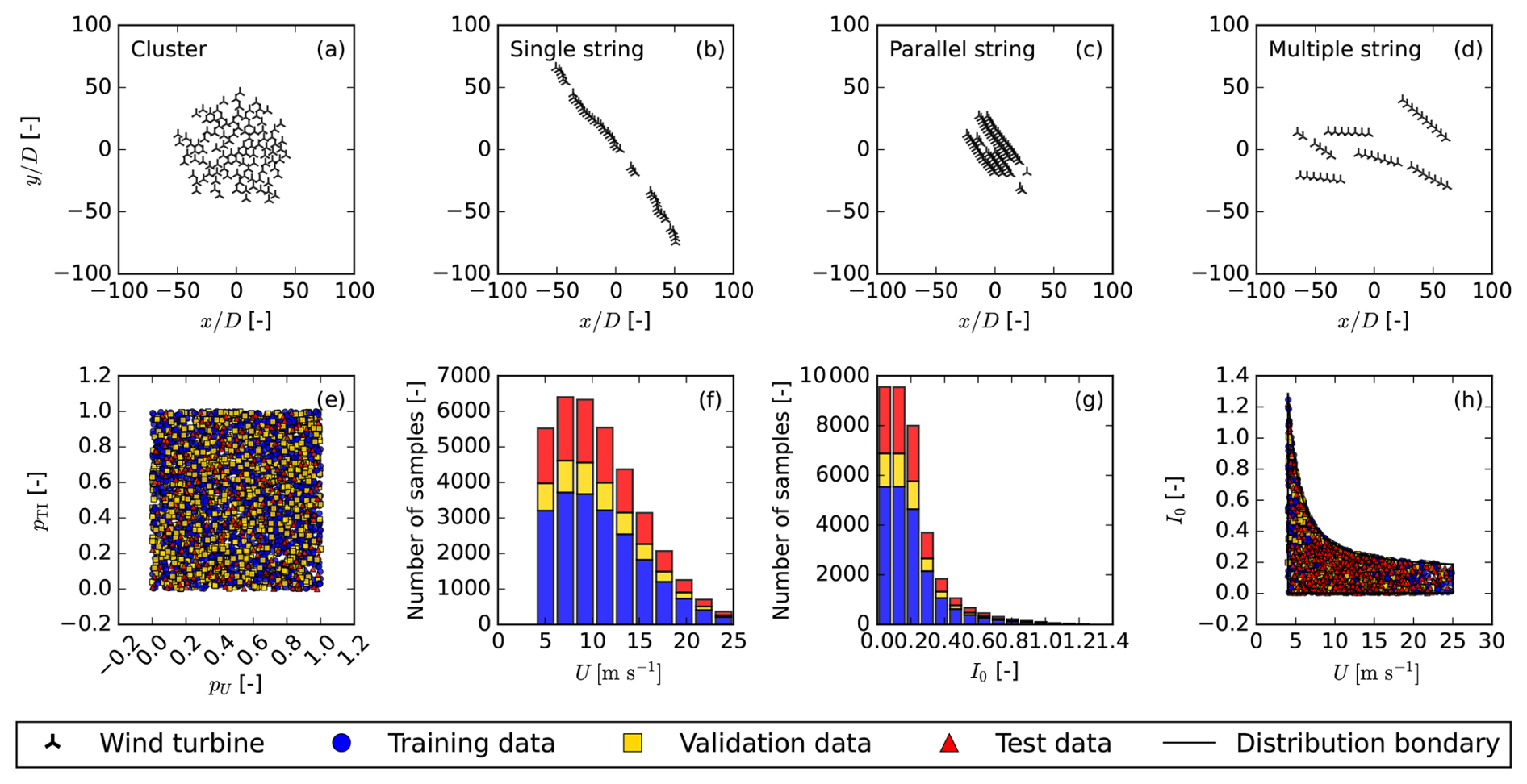
Figure 1 Procedurally generated data, (a–d) wind farm layouts using PlayGen. (e) Quasi-random samples generated with the Sobol sequence. (f) U distribution. (g) Ambient turbulence intensity (TI) distribution. (h) Generated U and I₀ with boundary.

Furthermore, a secondary contribution is the development of a data generation pipeline that combines state-of-the-art engineering models with stochastic sampling to produce physically realistic and diverse training data.

The article is structured as follows: Sect. 2 introduces the employed methods and is divided into four subsections: data generation, graphs, the GNO, and performance metrics. Section 3 consists of two parts: in Sect. 3.1, a summary of the results of a grid search to determine suitable hyperparameters is introduced; and in Sect. 3.2, the best-performing model is rigorously tested and discussed. Finally, in Sect. 4, conclusions and suggestions for future work are summarized.

2 Methodology

This section introduces the methods used to construct the GNO, create training data, and evaluate the model. In Sect. 2.1, the data generation process is described, covering random layout generation, inflow generation, and wind farm flow simulation. A general introduction to graphs is provided in Sect. 2.2, and subsequently, the proposed GNO is introduced in Sect. 2.3, including an overview of the neural network methods used to construct it. Finally, in Sect. 2.4, the methods for training and evaluation are described, along with the introduction of the performance metrics used.

2.1 Data generation

To ensure the dataset includes a representative subset of wind farm layouts and inflow conditions, these scenarios are procedurally generated. In total, 3570 unique layouts are generated. Ten inflow conditions per layout were selected to improve the neural network's ability to learn the correlation between inflow conditions and the wind farm wake deficit. A total of 2072 of the generated layouts are used for training, 500 are used for validation during training, and 998 layouts are set aside for testing. That means that for training, 20 720 data points are considered – 5000 for validation and 9980 for testing.

2.1.1 Layout generation

Plant Layout Generator (PlayGen) by Harrison-Atlas et al. (2024) is used to generate wind farm layouts. PlayGen creates four types of layouts: Cluster, which uses Poisson disk sampling to iteratively generate the wind farms by selecting an existing turbine, generating a random angle and distance, and placing the new turbine if it satisfies the spacing constraints. Single string creates linear turbine arrays with inserted breaks, applies cumulative correlated noise to y coordinates, and rotates the entire string. Parallel string makes multiple linear strings with the same orientation and vertically offsets each string by 1 to 3.5 rotor diameters (D). Then it applies random horizontal shifts and rotates the full layout. Multi string distributes turbines across strings, each with a quasi-random independent orientation, and places them in a domain while checking for string spacing. Examples of these are plotted in Fig. 1a–d.

The layout type, number of wind turbines (n_wt) and turbine separation factors (s_wt) are sampled according to the probabilities and distributions listed below:

• Farm type: categorical distribution sampled with probabilities P_farm

  $$P_{\text{farm}}=\left[\begin{array}{c}{P}_{\text{cluster}}\\ P_{\text{single\hspace{0.17em}\hspace{0.17em}string}}\\ P_{\text{parallel\hspace{0.17em}\hspace{0.17em}string}}\\ P_{\text{multiple\hspace{0.17em}\hspace{0.17em}string}}\end{array}\right]=\left[\begin{array}{c}\mathrm{0.40}\\ \mathrm{0.20}\\ \mathrm{0.20}\\ \mathrm{0.20}\end{array}\right].$$

• Number of wind turbines n_wt∈ℤ sampled with a truncated normal distribution TN

  $$n_{\text{wt}}\sim \text{TN}(\mathit{\mu }=\mathrm{60},\mathit{\sigma }=\mathrm{60},{\mathit{\delta }}_{\text{low}}=\mathrm{20},{\mathit{\delta }}_{\text{high}}=\mathrm{100}).$$

• Wind turbine separation factor $s_{\text{wt}}\in {\mathbb{R}}_{\mathrm{0}}^{+}$ sampled with a truncated normal distribution TN

  $$s_{\text{wt}}\sim \text{TN}(\mathit{\mu }=\mathrm{5}D,\mathit{\sigma }=\mathrm{3}D,{\mathit{\delta }}_{\text{low}}=\mathrm{2}D,{\mathit{\delta }}_{\text{high}}=\mathrm{8}D).$$

where P are probabilities and subscripts indicate the layout type considered, μ is the mean, σ the standard deviation, δ_low the lower cut-off, and δ_high the upper cut-off for the truncated normal distribution TN.

2.1.2 Inflow generation

The inflow conditions required for the wind farm simulation are the free-stream velocity and ambient turbulence intensity, respectively, in the variables U and I₀. As these are naturally highly correlated, it is necessary to consider this when generating the flow cases. The methods of Dimitrov et al. (2018) are used to generate correlated inflow conditions. After Dimitrov et al. (2018) was initially published, IEC 61400-1:2019 ed. 4 (2019) has been updated with a slight change to the classifications of turbulence characteristics. Therefore, the new A⁺ class is used with reference turbulence intensity ($I_{\text{ref},{\mathrm{A}}^{+}}=\mathrm{0.18}$). Ranges of the free-stream velocity are based on the DTU-10-MW reference wind turbine (Bak et al., 2013) with rotor diameter (D = 178.3 m), cut-in (U_c,in = 4 m s⁻¹), rated (U_rated = 11.4 m s⁻¹), and cut-out (U_c,out = 25 m s⁻¹) wind speeds. The power curve and coefficient of thrust (C_T) curves of the DTU-10-MW are displayed in Fig. 2. The velocity standard deviation (σ_u) lower and upper bounds follow the expressions in Dimitrov et al. (2018; Table 1). The expressions for the inflow bounds are given in Eq. (1).

$$\begin{array}{}\text{(1a)}& {\displaystyle }\mathrm{4}\mathrm{m}{\mathrm{s}}^{-\mathrm{1}}\le U\le \mathrm{25}\mathrm{m}{\mathrm{s}}^{-\mathrm{1}}\text{(1b)}& {\displaystyle }\begin{array}{rl}\mathrm{0.0025}\cdot U\le & {\mathit{\sigma }}_{\mathrm{u}}\le I_{\text{ref},{\mathrm{A}}^{+}}\left(\mathrm{6.8}+{\displaystyle \frac{\mathrm{3}U}{\mathrm{4}}}+\mathrm{3}{\left({\displaystyle \frac{\mathrm{10}}{U}}\right)}^{\mathrm{2}}\right)\\ & \left[\mathrm{m}{\mathrm{s}}^{-\mathrm{1}}\right]\end{array}\end{array}$$

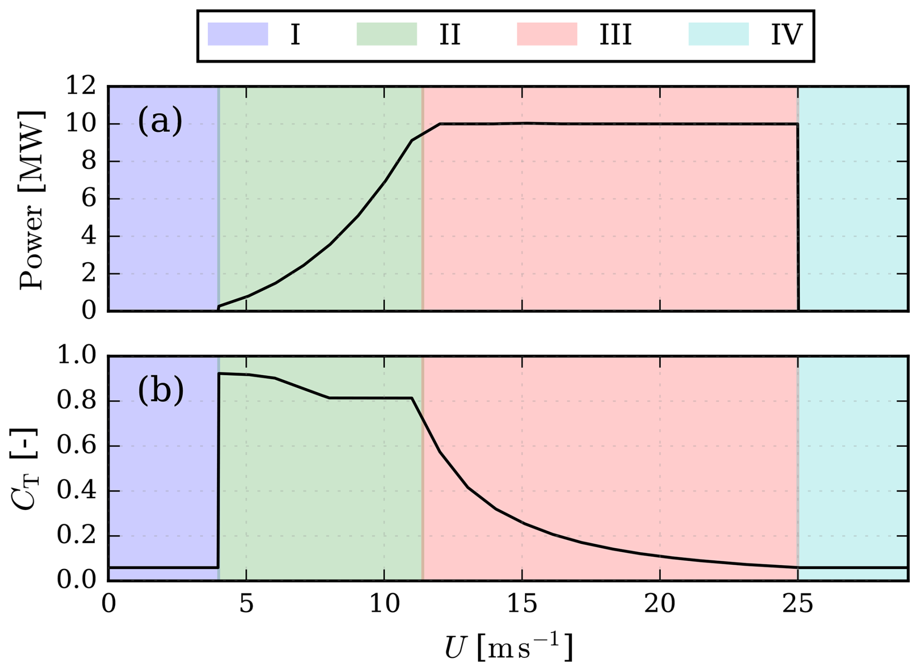
Figure 2 DTU-10-MW reference wind turbine (a) power curve and (b) C_T curve as implemented in PyWake. Operational stages I–IV are indicated with colors. I: below cut-in, II: below rated power, III: rated power, and IV: above cut-out.

Correlated inflow conditions are generated using quasi-Monte-Carlo sampling with the improved Sobol sequence (Joe and Kuo, 2008). While Dimitrov et al. (2018) employed the Halton sequence for similar purposes, we tested both approaches and found that the Sobol sequence, also used by de Santos et al. (2024), better captures extreme values in the distribution tails.

Figure 1e illustrates the two-dimensional quasi-random samples from the Sobol sequence before transformation. The sampled component used to generate the free-stream velocity U is denoted as p_U, and p_TI denotes the component used to generate the ambient TI. In Fig. 1f, the resultant wind speed distribution is shown. The distribution was obtained by projecting the wind speed sample onto a Rayleigh distribution following IEC 61400-1:2019 ed. 4 (2019) and scaled with the range in Eq. (1a). To obtain the resultant TI distribution, Eq. (1b) is applied, and the turbulence standard deviation is converted to TI by the relation $I={\mathit{\sigma }}_{\mathrm{u}}/U$ (the TI distribution is shown in Fig. 1g as a histogram).

2.1.3 Wind farm simulation

The dataset is generated with the wind farm simulation tool PyWake (Pedersen et al., 2023). PyWake is an open-source steady-state engineering wake modeling framework that computes wake deficits and turbine interactions. The framework supports spatially varying inflow conditions, multiple turbine types, and yaw misalignment via wake deflection models. However, to establish a baseline dataset, several simplifications were adopted: (i) homogeneous inflow with uniform free-stream velocity and turbulence intensity, (ii) a single turbine type (DTU-10-MW) with a fixed C_T curve, and (iii) all turbines aligned with the inflow direction. These choices reduce the input parameter space but may limit applicability to scenarios involving heterogeneous inflows, mixed turbine fleets, or active wake control.

The wakes are modeled with the updated self-similar Gaussian single-wake deficit model NiayifarGaussianDeficit by Niayifar and Porté-Agel (2016), which is a further development of the Gaussian wake model by Bastankhah and Porté-Agel (2014). This model was chosen for its TI-dependent wake expansion, which ensures coupling between TI and velocity deficits. The model uses an adaptive wake growth rate (k^∗) that is linearly fit to the wind turbine inflow TI (I_wt) immediately upstream of each turbine. Therefore, it requires an added TI (I_a) model; here, the CrespoHernandez model by Crespo and Hernández (1996) was chosen. Additionally, to account for the effects of turbine induction, the updated self-similarity blockage model SelfSimilarityDeficit2020 by Troldborg and Meyer Forsting (2017) and Forsting et al. (2023) is used. Finally, to superpose wakes and induction together, a linear sum is used. The effective velocity (u) at turbine number i is computed as

$$\begin{array}{}\text{(2)}& u_{\mathrm{i}}=U-\sum _{j=\mathrm{1}}^{N_{\text{up}}}\mathrm{\Delta }{u}_j-\sum _{k=\mathrm{1}}^{N_{\text{down}}}\mathrm{\Delta }{u}_{b,k},\end{array}$$

where Δu is the velocity deficit caused by wake effects, Δu_b is the wake deficit caused by blockage, j sums across all turbines upstream of turbine i, and k sums across all turbines downstream of turbine i. For the interested reader, the velocity deficit model, TI model, and blockage model are presented in detail in Appendix A.

To obtain the state of the wind farm, the All2AllIterative wind farm model is used, in which a local reference wind speed u_ref is calculated per wind turbine. The inter-turbine effects are iteratively evaluated using fixed-point iteration until a convergence criterion is met. Using All2AllIterative is necessary when a blockage model is included, as the turbines interact in both upstream and downstream directions. After the dataset for this work was generated, a computationally lighter alternative wind farm model, the PropagateUpDownIterative model, was implemented in PyWake. This model can significantly accelerate dataset generation, and the authors encourage its adoption in future studies.

However, the use of All2AllIterative also benefits the GNO application: because turbine interactions are resolved iteratively in both directions, the resulting input–output mapping constitutes a nonlinear operator, providing a more challenging and representative test case for the GNO than a simple PropagateDownwind scheme. Although PyWake employs linear wake superposition (Eq. 2), the coupled iterative solution introduces nonlinearity that the GNO must learn to approximate. More broadly, the dataset was designed to capture diverse physical effects, including blockage, turbulence-dependent wake expansion, and bidirectional interactions, rather than to maximize fidelity to any single high-accuracy model. Such diversity ensures that the GNO learns a sufficiently complex operator, demonstrating its capacity to generalize across varied flow physics. Future work should investigate the impact of both different superposition methodologies and higher-fidelity training data on GNO performance.

One of the strengths of the GNO is its grid invariance: once the turbine operating states are determined, flow predictions can be queried at arbitrary locations. This allows the simulated area to be strategically chosen to capture wake dynamics while avoiding redundant data from unwaked regions. Therefore, a bounding box is constructed to fit each farm. For each farm layout, the wind turbines with the minimum and maximum downstream x and cross-stream y coordinates are found and padded as follows:

• Downstream: (x direction) an extension of 100D behind the most downstream turbine,

• Upstream: (x direction) an extension of 10D in front of the most upstream turbine,

• Cross-stream: (y direction) an extension of 5D on each side.

Figure 3 illustrates the bounding box of a wind farm. A farm downstream axis $\stackrel{\mathrm{̃}}{x}$ is introduced to measure the distance behind the most downstream turbine, making it easier to compare results across different wind farm layouts. The flow map is constructed to remain within the bounding box, at a single height – the turbine hub height (z_hub = 119 m). The flow map uses an isotropic grid resolution of 3 points per D. For each layout and sampled inflow case, the computed effective turbine velocities and the velocities at the pre-determined grid locations are recorded. As an artifact of the PlayGen generation methods, the wind farm center and coordinate center do not always coincide. Because the GNO uses relative internal coordinates, this does not affect its performance; more details are given in Sect. 2.2.

Figure 3 Adaptive computational grid for generating flow maps with PyWake.

2.2 Graphs

Graph theory was introduced by Euler (1741) to address the Königsberg bridge problem. Euler modeled land masses as nodes (v) and bridges as edges (e) in a graph. Although simple compared to modern graphs, this representation enabled Euler to mathematically prove the impossibility of solving the Königsberg bridge problem.

Graphs are powerful tools for representing data. They consist of nodes (or vertices), edges, and optionally global features. Nodes hold values representing information such as positions and states, while edges represent relationships or interactions between nodes and may also carry additional attributes, referred to as edge features. Global features, in turn, apply to the entire graph and are often used in graph classification tasks. In this work, global features are not included directly; instead, following the approach of Duthé et al. (2023), they are copied to each node as node features.

The notation in this work uses both set theory and vector notation, depending on which is more appropriate in a given context. In set notation, the nodes are represented by V and the edges by E, with the graph represented as $G=(V,E)$. In vector notation, the nodes are denoted by v, with individual vector elements represented as v_i; similarly, the edges are denoted by e, with individual elements represented as e_i. Set theory is primarily used to express the cardinality of these sets – that is, the number of elements they contain, written as $\left|V\right|$ and $\left|E\right|$. The use of cardinality highlights the fact that the numbers of nodes and edges are not fixed, which is a strength of graphs but also makes the notation more complicated.

In our implementation, two types of nodes are considered: wind turbine nodes (V_wt) and probe nodes (V_p), where

$$\begin{array}{}\text{(3)}& V=V_{\text{wt}}\cup V_{\mathrm{p}}.\end{array}$$

Wind turbine nodes coincide with the physical turbine positions in the farm, while probe nodes correspond to locations where flow predictions are desired, i.e., points in space at which the flow is evaluated. Similarly, the edges are separated into two inter-turbine edges (E_wt) and those connecting wind turbines and nodes (E_p), both a subset of E.

$$\begin{array}{}\text{(4)}& E=E_{\text{wt}}\cup E_{\mathrm{p}}\end{array}$$

The edges store the relative node positions (x_ij and y_ij) and Euclidean distance (d_ij) between connected nodes:

$$\begin{array}{}\text{(5)}& (x_{ij},y_{ij},d_{ij})=\left(x_{\mathrm{j}}-x_{\mathrm{i}},y_{\mathrm{j}}-y_{\mathrm{i}},\sqrt{x_{ij}^{\mathrm{2}}+y_{ij}^{\mathrm{2}}}\right).\end{array}$$

The inter-turbine edges are bidirectional, enabling message passing in both directions. This corresponds to solving for turbine thrust coefficients in traditional wake modeling, and the resulting latent space can be thought of as a high-dimensional representation of the turbine thrust states.

By contrast, edges connecting to probe nodes are unidirectional, with each probe node connected to and receiving from all wind turbine nodes. This corresponds to using a wake simulation result to predict a resulting flow map when the turbine thrust states are already set.

Probe node connectivity is straightforward because each probe connects to all wind turbines. Inter-turbine connectivity is more complex because it requires an algorithmic approach to determine which turbines should be connected. Several algorithms exist for constructing the connectivity of the turbine nodes. Duthé et al. (2023) investigated four graph connectivity schemes: Delaunay triangulation (Delaunay, 1934; O'Rourke, 1988; Fey and Lenssen, 2019), K-nearest neighbors (KNN), a radius-based method, and a fully connected scheme. They concluded that Delaunay triangulation provides the best balance between accuracy and computational performance. Accordingly, we also adopt Delaunay triangulation in this work to derive inter-turbine connections.

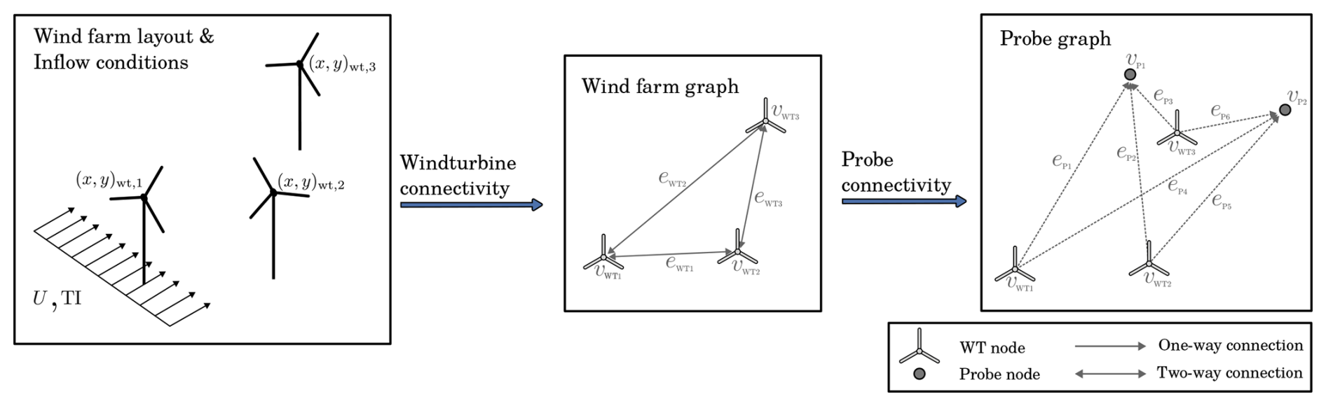
Figure 4 An example of constructing graph connectivity with three wind turbines and two probes, given a layout and inflow.

An example of the graph construction process is illustrated in Fig. 4, where the process of establishing the connectivity of the wind farm graph and the probe graph is separated into two stages. In our formulation, the edges include three features (f_e=3) as described in Eq. (5). Initially, wind turbine nodes store two features (f_v=2): the global wind speed U and the ambient I₀. No unique information is stored directly on the nodes; instead, global features are initially seeded and replicated across the nodes as part of the processing. Since the desired output is the wind speed at probe nodes, this constitutes a node task.

2.3 Graph neural operator (GNO)

The graph neural operator (GNO) is a special case of a GNN designed for learning mappings between function spaces. Li et al. (2020b) first introduced GNOs for this purpose. Building on this foundation, Sun et al. (2022) developed the deep graph operator network (DeepGraphONet), which integrates the deep operator network (DeepONet) architecture of Lu et al. (2021) with message-passing GNNs (Scarselli et al., 2009; Gilmer et al., 2017). The present work adopts the DeepGraphONet framework and extends it using the Nonlinear Manifold Decoder (NOMAD) formulation proposed by Seidman et al. (2022). NOMAD generalizes neural operators to fit into the encoder-processor-decoder abstraction.

Seidman et al. (2022) propose that an operator 𝒢 can be approximated as ℱ using an encoder ℰ, an approximator 𝒜, and a decoder 𝒟. The approximation ℱ can be written as a composition of the model components using the composition operator ∘, where the rightmost function is applied first.

$$\begin{array}{}\text{(6)}& \mathcal{G}\approx \mathcal{F}=\mathcal{D}\circ \mathcal{A}\circ \mathcal{E}\end{array}$$

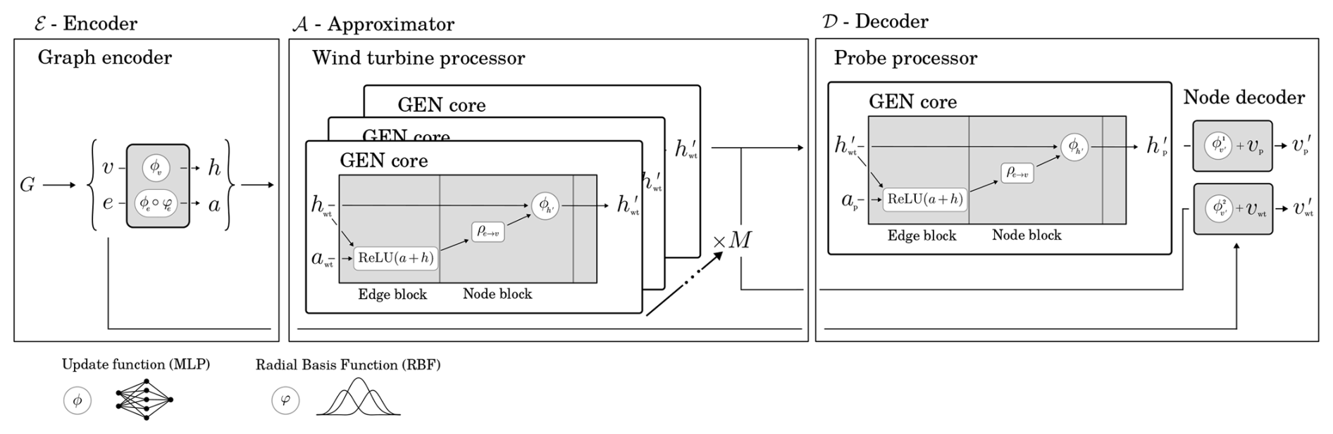
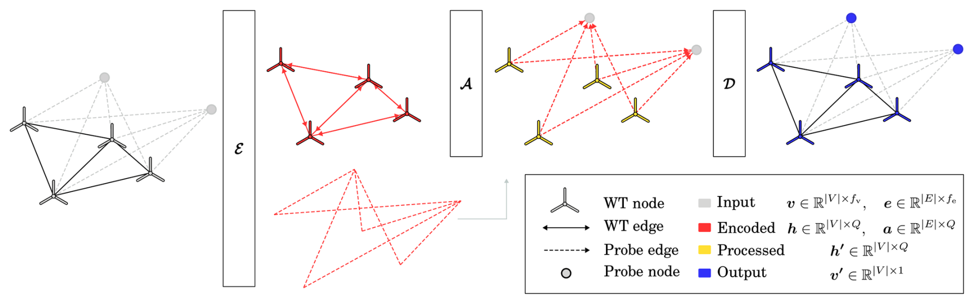
Figure 5 GNO network overview of its three main components: encoder, approximator, and decoder.

The encoder–approximator–decoder configuration is a widely adopted architectural pattern in GNNs, providing a modular framework for transforming input graphs into predictions (Battaglia et al., 2018). In Fig. 5, an overview of the considered model is shown, while the encoder and approximator stages conceptually are equivalent to most GNNs. The final decoder stage stands out as the decoder includes a variation of a readout that uses a separate set of featured probe edges E_p. By including E_p, the relative position of the turbines to the probe location is included during the readout. Additionally, due to the separation of probe node processing and the simplicity of establishing probe connectivity, probes can be created on the fly without re-establishing wind turbine connections, i.e., E_wt, or reprocessing the wind turbine nodes. This means that predicting in a flow field incurs lower computational cost than a fully integrated prediction scenario.

As previously discussed, the structure of the GNO mirrors the modeling flow of engineering-based wind farm models. In such models, a connectivity matrix is established based on the spatial layout of the turbines and the chosen wake interaction scheme. For instance, in fully coupled formulations, all turbines influence one another, and the initial state is defined by the undisturbed inflow conditions. Analogously, the GNO constructs a graph representation of the wind farm, which is then encoded into an initial higher-order thrust state. The approximator within the GNO can be interpreted as analogous to the iterative update process used in conventional wake models to adjust individual turbine states. However, in the GNO framework, this computation is performed in a latent space rather than directly in the physical domain. Finally, the decoder evaluates the aggregated flow response of the wind farm, corresponding to the reconstruction of a flow field or flow map in traditional engineering approaches. These parallels are made explicit in Eq. (6), where the constitutive components of the GNO reflect the sequential structure of conventional wind farm modeling frameworks.

2.3.1 Encoding

The graph encoder layer ℰ consists of parallel encoders for nodes and edges. The nodes are encoded with an MLP, and the edges are encoded in two steps: first, they are pre-processed with radial basis functions (RBFs) and then encoded to the target latent space with an MLP. It is well known that there are different flow regimes at various downstream distances from a turbine. RBFs are used to encourage the network to view different downstream distances as distinct regimes. In initial experimentation, it was found to improve training. The input edge and node data are projected into latent spaces of the same dimensionality, denoted as Q, ensuring dimensional consistency as the chosen approximator core – GEneralized Aggregation Network (GEN) – requires equal latent-space dimensions for nodes and edges. This is because the node and edge features are added together in the latent space.

The structure of an MLP is described in three stages: the input layer in Eq. (7a), the hidden layers in Eq. (7b), and the output layer in Eq. (7c).

$$\begin{array}{}\text{(7a)}& {\displaystyle }& {\displaystyle }{\mathit{\xi }}^{\left(\mathrm{0}\right)}=\mathit{\psi }\left({\mathbf{W}}^{\left(\mathrm{0}\right)\top }\mathit{x}+{\mathit{b}}^{\left(\mathrm{0}\right)}\right)\text{(7b)}& {\displaystyle }& {\displaystyle }{\mathit{\xi }}^{\left(l\right)}=\mathit{\psi }\left({\mathbf{W}}^{\left(l\right)\top }{\mathit{\xi }}^{(l-\mathrm{1})}+{\mathit{b}}^{\left(l\right)}\right),l=\mathrm{1},\mathrm{2},\mathrm{\dots },L-\mathrm{1}\text{(7c)}& {\displaystyle }& {\displaystyle }\mathit{\varphi }\left(\mathit{x}\right)={\mathbf{W}}^{\left(L\right)\top }{\mathit{\xi }}^{(L-\mathrm{1})}+{\mathit{b}}^{\left(L\right)},\end{array}$$

where ϕ(x) represents the overall MLP mapping for input vector x; ξ^(l) denotes the hidden units at layer l; W^(l) and b^(l) are the weights and biases of the network, respectively; and ψ is the activation function. In this work, the activation function is the Rectified Linear Unit (ReLU). The MLPs considered in this work operate in real space and are used to map between different dimensions in both the latent and observational spaces, i.e., $\mathit{\varphi }:{\mathbb{R}}^{N\times C}\to {\mathbb{R}}^{N\times Q}\forall N,C,Q\in \mathbb{N}$.

RBFs are used to map the initial edge features, here distances between wind turbines i and j (d_ij), into a higher-dimensional space. We employ K=9 Gaussian basis functions to transform distances such that $\mathit{\phi }:{\mathbb{R}}^{\mathrm{1}}\to {\mathbb{R}}^K$. The formulation of the RBF is shown in Eq. (8):

$$\begin{array}{}\text{(8a)}& {\displaystyle }\begin{array}{rl}\mathit{\phi }\left(d_{ij}\right)=\exp \left(-{\mathit{\beta }}_{\text{RBF}}^{\left(k\right)}{\left(d_{ij}-{\mathit{\mu }}_{\text{RBF}}^{\left(k\right)}\right)}^{\mathrm{2}}\right)& \cdot {\mathit{\delta }}_{\mathrm{c}}\left(d_{ij}\right),\\ & k=\mathrm{1},\mathrm{\dots },K,\end{array}\text{(8b)}& {\displaystyle }{\mathit{\delta }}_{\mathrm{c}}\left(d_{ij}\right)=\left\{\begin{array}{ll}\mathrm{0.5}\cdot \left[\cos \left({\displaystyle \frac{\mathit{\pi }{d}_{ij}}{d_c}}\right)+\mathrm{1}\right],& \text{for }{d}_{ij}\le d_c,\\ \mathrm{0},& \text{for }{d}_{ij}>d_c,\end{array}\right.\end{array}$$

where ${\mathit{\beta }}_{\text{RBF}}^{\left(k\right)}$ and ${\mathit{\mu }}_{\text{RBF}}^{\left(k\right)}$ are trainable parameters defining the kth basis function, and δ_c(d_ij) is a cosine cut-off function with cut-off distance d_c≈695 D, chosen as the diagonal of the largest flow map to ensure that no edge is fully ignored. A more aggressive cut-off could be adopted in the future but would require a dedicated study to determine an appropriate value. The initial ${\mathit{\mu }}_{\text{RBF}}^{\left(k\right)}$ are linearly spaced between −1 and 1, while ${\mathit{\beta }}_{\text{RBF}}^{\left(k\right)}$ all are initialized based on the maximum range and number of basis functions ${\mathit{\beta }}_{\text{RBF}}^{\left(k\right)}=\frac{K}{max\left(d_{ij}\right)-min\left(d_{ij}\right)}$. The addition of RBF functions to encode the distances is inspired by the work of Jørgensen and Bhowmik (2022), who used it in their GNN for electron density estimation.

Combined, the encoding steps are summarized in Eq. (9):

$$\begin{array}{}\text{(9a)}& {\displaystyle }& {\displaystyle }\mathit{h}={\mathit{\varphi }}_{\mathrm{v}}\left(\mathit{v}\right),\text{(9b)}& {\displaystyle }& {\displaystyle }\mathit{a}=({\mathit{\varphi }}_{\mathrm{e}}\circ {\mathit{\phi }}_{\mathrm{e}})\left(\mathit{e}\right),\end{array}$$

where h and a denote the latent-space representations of nodes and edges, respectively. ${\mathit{\phi }}_e:{\mathbb{R}}^{\left|E\right|\times f_{\mathrm{e}}}\to {\mathbb{R}}^{\left|V\right|\times f_{\mathrm{e}}\cdot K}$ is the RBF function mapping each edge feature from the initial observational space to a K dimensional RBF space, and ${\mathit{\varphi }}_v:{\mathbb{R}}^{\left|V\right|\times f_{\mathrm{v}}}\to {\mathbb{R}}^{\left|V\right|\times Q}$ and ${\mathit{\varphi }}_e:{\mathbb{R}}^{\left|E\right|\times f_{\mathrm{e}}K}\to {\mathbb{R}}^{\left|E\right|\times Q}$ are the node and edge encoding MLPs. For convenience, the key dimensions are restated here: the cardinalities $\left|V\right|$ and $\left|E\right|$ vary with the wind farm configuration; f_v=2 and f_e=3 are the initial node and edge feature dimensions; K=9 is the number of RBF kernels; and Q is the latent-space dimension.

2.3.2 Approximator: GEneralized Aggregation Network (GEN)

The central component of the GNO is the approximator 𝒜. It applies the GEN message-passing algorithm by Li et al. (2020a), with three message-passing steps (M=3) sequentially applied on the encoded latent-space wind turbine nodes (h_wt) using the latent-space inter-turbine edges (a_wt) to obtain the processed wind turbine nodes (${{\mathit{h}}^{\mathbf{\prime }}}_{\text{wt}}$).

The GEN methodology consists of the construction of the messages (m_ij), the application of the edge-to-node aggregation function (ρ_e→v), and the node update MLP (ϕ_v):

$$\begin{array}{}\text{(10a)}& {\displaystyle }{\mathit{m}}_{ij}^{\left(m\right)}=\text{ReLU}\left({\mathit{h}}_j^{\left(m\right)}+{\mathit{a}}_{\text{ji}}\right)+\mathit{\epsilon },j\in \mathcal{N}\left(i\right)\text{(10b)}& {\displaystyle }\begin{array}{rl}{\mathit{h}}_i^{(m+\mathrm{1})}=& {\mathit{\varphi }}_{h^{\prime }}^{\left(m\right)}\left({\mathit{h}}_i^{\left(m\right)}+{\mathit{\rho }}_{e\to v}\left({\mathit{m}}_{ij}^{\left(m\right)}\right)\right),\\ & m=\mathrm{1},\mathrm{2}\mathrm{\dots }M,\end{array}\end{array}$$

where m is the current message-passing step, and i∈ℐ is the index of a receiving node, with ℐ being an index set relating to all receiving nodes. Correspondingly, j indicates a sending node, 𝒩(i) is a set of the nodes neighboring the node with index i, and $\mathit{\epsilon }=\mathrm{1}\times {\mathrm{10}}^{-\mathrm{6}}$ is a small positive value added for numerical stability. In Fig. 5, the GEN core is visualized schematically. In this work, Softmax aggregation is used as ρ_e→v; it uses Softmax to scale the latent space of each feature dimension independently. The incoming messages to node i from its $\left|\mathcal{N}\right(i\left)\right|$ neighbors form a matrix of shape $\left|\mathcal{N}\right(i\left)\right|\times Q$. For each feature dimension, let ${\widehat{\mathit{x}}}_{\mathrm{q}}\in {\mathbb{R}}^{\left|\mathcal{N}\right(i\left)\right|}$ denote the vector containing the qth feature value across all neighbors.

$$\begin{array}{}\text{(11)}& {\mathit{\rho }}_{e\to v}=\sum _{{\widehat{\mathit{x}}}_{\mathrm{q}}\in \mathcal{X}}{\displaystyle \frac{\exp \left({\widehat{\mathit{x}}}_{\mathrm{q}}\right)}{{\sum }_{{\widehat{\mathit{x}}}_{\mathrm{r}}\in \mathcal{X}}\exp \left({\widehat{\mathit{x}}}_{\mathrm{r}}\right)}}\cdot {\widehat{\mathit{x}}}_{\mathrm{q}},\end{array}$$

where $\mathcal{X}=\mathit{\{}{\widehat{\mathit{x}}}_{\mathrm{1}},\mathrm{\dots },{\widehat{\mathit{x}}}_{\mathrm{Q}}\mathit{\}}$ is a collection of neighborhood features to be aggregated independently.

Figure 6 GNO Probe input, processing and output with model data flow from left to right.

2.3.3 Decoder

In the first part of the decoder stage (𝒟), an additional message-passing step is performed using the processed wind turbine nodes ${{\mathit{h}}^{\mathbf{\prime }}}_{\text{wt}}$ with the latent-space probe edges a_p to obtain processed probe nodes ${{\mathit{h}}^{\mathbf{\prime }}}_{\mathrm{p}}$, consisting of aggregated information from all the wind turbine nodes. In the final part of the decoder stage, two separate MLPs map the latent variables back to the observational space. A residual-network (ResNet) formulation is adopted, in which the free-stream velocity U is added to the decoded node values as the final step during inference. Consequently, this residual connection is also taken into account during the evaluation of the loss function during training.

$$\begin{array}{}\text{(12a)}& {\displaystyle }& {\displaystyle }{{\mathit{v}}^{\mathbf{\prime }}}_{\mathrm{p}}={\mathit{\varphi }}_{v^{\prime }}^{\left(\mathrm{1}\right)}\left({{\mathit{h}}^{\mathbf{\prime }}}_{\mathrm{p}}\right)+{\mathit{v}}_{\mathrm{p}},\text{(12b)}& {\displaystyle }& {\displaystyle }{{\mathit{v}}^{\mathbf{\prime }}}_{\text{wt}}={\mathit{\varphi }}_{v^{\prime }}^{\left(\mathrm{2}\right)}\left({{\mathit{h}}^{\mathbf{\prime }}}_{\text{wt}}\right)+{\mathit{v}}_{\text{wt}},\end{array}$$

where ${\mathit{\varphi }}_{v^{\prime }}^{\left(\mathrm{1}\right)}$ and ${\mathit{\varphi }}_{v^{\prime }}^{\left(\mathrm{2}\right)}$ are the decoding MLPs, both mapping from the latent space to the output space:
${\mathit{\varphi }}_{v^{\prime }}^{\left(\mathrm{1}\right)},{\mathit{\varphi }}_{v^{\prime }}^{\left(\mathrm{2}\right)}:{\mathbb{R}}^{\left|V_{\mathrm{p}}\right|\times Q},{\mathbb{R}}^{\left|V_{\text{wt}}\right|\times Q}\to {\mathbb{R}}^{\left|V_{\mathrm{p}}\right|\times \mathrm{1}},{\mathbb{R}}^{\left|V_{\text{wt}}\right|\times \mathrm{1}}$. Here, v_p, ${{\mathit{h}}^{\mathbf{\prime }}}_{\mathrm{p}}$, and ${{\mathit{v}}^{\mathbf{\prime }}}_{\mathrm{p}}$ denote the probe input nodes, hidden-state nodes, and predictions, respectively. Likewise, v_wt, ${{\mathit{h}}^{\mathbf{\prime }}}_{\text{wt}}$, and ${{\mathit{v}}^{\mathbf{\prime }}}_{\text{wt}}$ correspond to the wind turbine input nodes, hidden-state nodes, and predictions.

The data flow through the GNO is shown in Fig. 6, where the components defined in Eq. (6) and described in this subsection are represented as boxes. The partially processed graph states are distinguished by color, providing a visual overview of the GNO architecture and its internal data transformations.

2.3.4 Regularization and normalization

With the layered nature of the GNO model, the total number of layers grows fast; with deep models, it is advisable to include regularization and normalization to avoid overfitting. In this work, both the node and edge features are scaled, meaning wind speeds, TI, and positional information. Additionally, layer normalization and dropout regularization are used inside the GNO. For feature scaling, range normalization is used.

$$\begin{array}{}\text{(13)}& {\mathit{\vartheta }}^{\prime }={\displaystyle \frac{\mathit{\vartheta }}{max\left(\mathit{\vartheta }\right)-min\left(\mathit{\vartheta }\right)}},\end{array}$$

where ϑ is an unscaled feature and ϑ^′ is the respective scaled feature. The features are only scaled by the feature range as it allows ResNet application inside the scaled feature space, which makes model implementation easier.

To counter overfitting, dropout regularization, as implemented by Srivastava et al. (2014), has been incorporated into our MLP formulation. Dropout works by randomly omitting the output of some neurons during training, making the network more robust and reducing the risk of over-reliance on single neurons. A dropout probability of P_D=0.1 has been used in this study; further implementation details can be found in Appendix B.

A common technique to improve training stability and speed up training is batch normalization. However, as the trained GNO can handle graphs of any size, there is no fixed batch size, which makes batch statistics unreliable. Additionally, during training, graphs are batched together, and statistics across graphs are not desirable. For additional information about graph batching with GNOs, see Appendix C. Instead, layer normalization, as proposed by Ba et al. (2016), can be used. While often considered less effective than batch normalization, layer normalization is fully compatible with GNNs. Ba et al. (2016) originally introduced it for MLPs and recurrent neural networks, applying it between hidden layers. In this work, since GNNs can be interpreted as compositions of MLP layers, layer normalization is applied only to the final layer of each MLP within the encoder ℰ and approximator 𝒜 stages, as well as during the message-passing step of the decoder 𝒟 stage. It is not applied to the final node-decoder MLPs, where full expressive power at the output is desired. Implementation details can be found in Appendix B.

2.4 Training and evaluation

The GNO is intended as a surrogate model for a regression-type task. Since a true model exists to learn from, the most straightforward training method is offline supervised training. To train the GNO, the high-performance computing (HPC) cluster Sophia (Technical University of Denmark, 2019) at DTU has been used. Nodes with Quadro RTX 4000 GPU acceleration were employed.

The optimization algorithm employed during training is Adam (Kingma and Ba, 2014). Adam is a variant of stochastic gradient descent (SGD) that incorporates past gradients and a momentum term to compute parameter updates. Consequently, multiple hyperparameters control the relative weighting of these terms. In this work, the default momentum parameters are used. During training, the dataset is shuffled and passed through the training algorithm multiple times; one such pass is termed an epoch. During an epoch, when a graph is sampled, the probes are sub-sampled from the flow domain; in practice, a flattened list is sampled uniformly. The probe node sample size (n_p) can be considered to be a hyperparameter that has been the subject of investigation during a hyperparameter search. In our implementation, a maximum of 3000 epochs has been considered, although this limit has not been reached at any point.

During training, the model is continuously evaluated using the validation dataset. If the validation performance surpasses previous results at any time, the saved model weights and biases are updated. The validation evaluation is performed every fifth epoch to save computational resources. Unlike during training, the graphs are not shuffled, and the probe nodes remain the same across epochs.

2.4.1 Machine learning framework

To train the GNO, a combination of different Python-based frameworks is used. The GNN components are constructed with the libraries based on Jax (Bradbury et al., 2018); Jraph is used for (Godwin et al., 2020) for GNN abstractions, and Flax (Heek et al., 2024) for neural networks. Additionally, as the Jax ecosystem does not yet have a dedicated data pipeline, graph construction and subsequent data loading are handled using PyTorch Geometric (PyG) (Fey and Lenssen, 2019). For additional details on the data pipeline, see Appendix C.

2.4.2 Performance metrics

Once a set of GNO weights are obtained through training, the resultant GNO model has to be tested. To accurately assess performance, various performance metrics are considered. Four statistical measures are considered: the mean absolute error (MAE), the mean absolute normalized error (MANE), the mean square error (MSE), and the root mean square error (RMSE). They differ in the first two using an l¹ norm and the last two using an l² norm. MSE and MAE are used to compare models, while MANE and RMSE is chosen to evaluate the best model as they are more easily interpreted. While most metrics are standard, MANE is a custom variation of mean absolute percentage error (MAPE). Standard MAPE normalizes by the target value, which becomes problematic when targets approach zero, as can occur near heavily waked turbines where wake superposition overestimates the deficit. Normalizing by the wake deficit instead would cause similar issues in unwaked regions. To avoid this, MANE normalizes by the free-stream velocity, providing a more robust metric that still enables comparison across different inflow conditions. The primary reason for including multiple metrics is to facilitate cross-comparison with other works in the field, as there is no consensus on which metrics to use. The metrics considered here are shown in Eq. (14):

$$\begin{array}{}\text{(14a)}& {\displaystyle }& {\displaystyle }\text{MAE}={\displaystyle \frac{\mathrm{1}}{N}}{∥\mathit{u}-\widehat{\mathit{u}}∥}_{\mathrm{1}},\text{(14b)}& {\displaystyle }& {\displaystyle }\text{MANE}={\displaystyle \frac{\mathrm{1}}{N}}{∥{\displaystyle \frac{\mathit{u}-\widehat{\mathit{u}}}{\mathit{U}}}∥}_{\mathrm{1}}\cdot \mathrm{100}\mathit{\%}\text{(14c)}& {\displaystyle }& {\displaystyle }\mathcal{L}=\text{MSE}={\displaystyle \frac{\mathrm{1}}{N}}{∥\mathit{u}-\widehat{\mathit{u}}∥}_{\mathrm{2}}^{\mathrm{2}},\mathrm{RMSE}={\displaystyle \frac{\mathrm{1}}{\sqrt{N}}}{∥\mathit{u}-\widehat{\mathit{u}}∥}_{\mathrm{2}},\end{array}$$

where u represents the target velocities, $\widehat{\mathit{u}}$ indicates the predicted velocities, U is the corresponding inflow velocities, and N is the number of observations. MSE is used as the loss function (ℒ) during training, as shown in Eq. 14c.

In some cases, it is practical to compare graphs by their relative size; a common approach to do this is to add up the size of their constituent parts. This can be done with different scaling factors and norms; however, the most straightforward and common approach is a linear sum accounting for feature sizes. The cardinality of the graph tuple $\left|G\right|$ is therefore defined as

$$\begin{array}{}\text{(15)}& \left|G\right|\equiv \left(\right|V_{\text{wt}}|+|V_{\mathrm{p}}\left|\right)\cdot f_{\mathrm{v}}+\left(\right|E_{\text{wt}}|+|E_{\mathrm{p}}\left|\right)\cdot (\mathrm{1}+f_{\mathrm{e}}),\end{array}$$

where the term (1+f_e) accounts for the fact that each edge stores both its f_e features and an index pair identifying the connected nodes in the adjacency list representation.

2.4.3 IEA Wind 740-10-MW reference wind farm

To evaluate the model on an established benchmark, the IEA Wind 740-10-MW reference wind farm is employed. This site features both a regular and an irregular wind farm layout, corresponding respectively to a simple grid configuration and an optimized configuration designed to improve overall farm performance. Both layouts are tested under the same wind speed conditions as reported in the technical documentation by Kainz et al. (2024). The two layouts are shown in Fig. 7. As the GNO predicts wind speeds, not power, it is necessary to calculate power using the power curve of the DTU-10-MW, illustrated in Fig. 2a; as this is a static simulation, it is a simple operation.

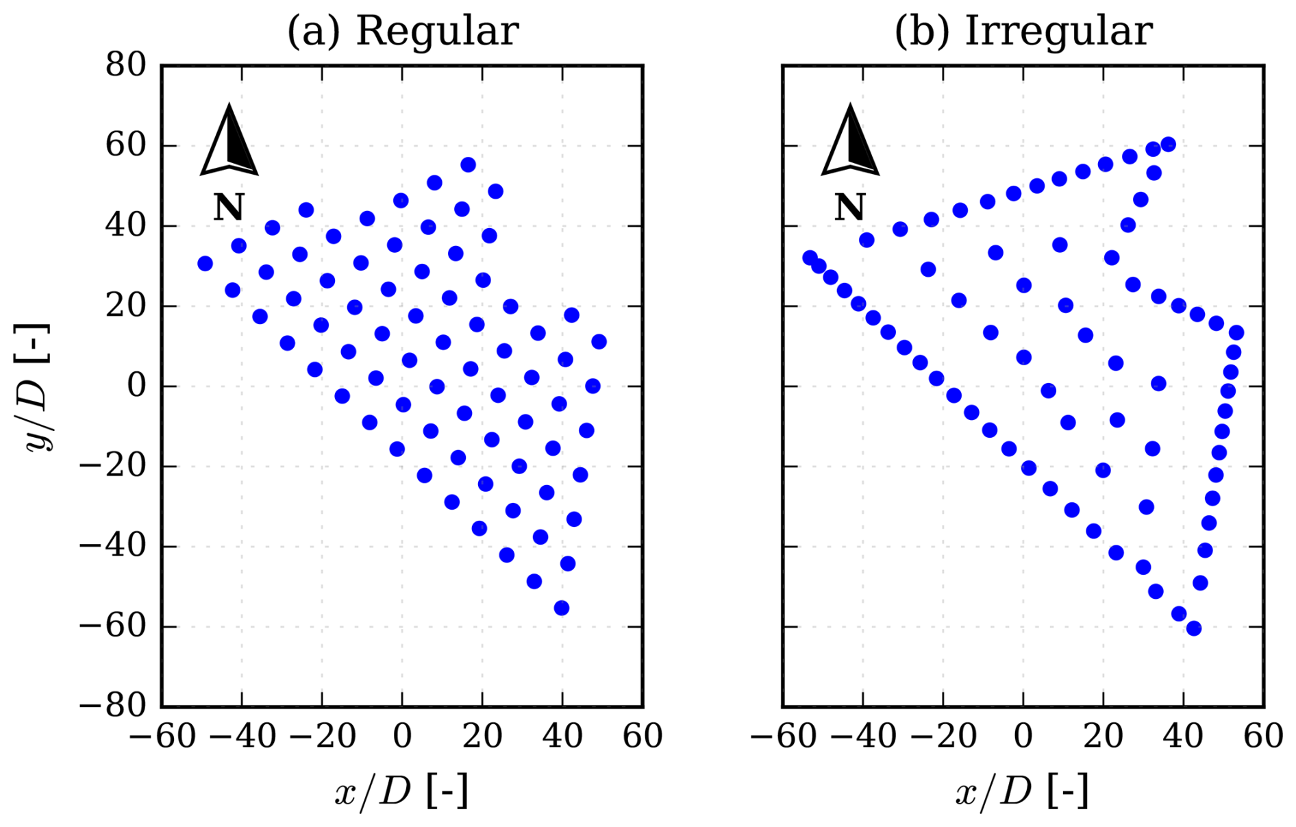
Figure 7 IEA Wind 740-10-MW reference wind farm (Kainz et al., 2024). (a) Regular layout pre-optimization and (b) irregular optimized layout.

3 Results and discussion

In this section, the results are presented and discussed concurrently. Initially, a summary of our hyperparameter grid search study is presented, followed by the selection of the best model, based on the validation data and its subsequent testing. The best-performing model is investigated separately, and a series of predictions are made using random layouts of each considered layout type. Both the probe node predictions and the wind turbine node predictions are investigated. Thereafter, a performance analysis is conducted, examining how errors are distributed across different input variables. Finally, the computational cost of the model is investigated and compared to the cost of PyWake.

3.1 Grid search

Neural network models consist of trainable parameters that are updated during training. In addition to these trainable parameters, preset parameters known as hyperparameters also define the model. The hyperparameters can be divided into two groups: the ones defining the model architecture and those specifying the optimization configuration. In this work, five consecutive grid searches were performed, with the results from each used to guide the subsequent search.

For the model configuration, the encoder, wind turbine processor, and probe processor MLPs are collectively referred to as the internal MLPs. The tested hyperparameters are the size of the latent dimension (Q), the number of layers in the internal MLPs (L_int), the number of neurons per layer in the internal MLPs (q_int), the number of hidden layers in the decoder MLP (L_dec), and the number of neurons per layer in the decoder (q_dec).

The considered optimization hyperparameters are the learning rate (LR) schedule, which falls into two main categories: constant and piecewise constant. An additional category, untriggered piecewise constant, indicates that the LR remained at its initial value throughout optimization. This occurs because the maximum wall time has been reached, and the training is stopped. This occurs in configurations with large input sizes because each training step takes longer and processes more data, requiring fewer epochs to converge.

In the piecewise constant schedule, the current LR is divided by 10 when a trigger step is reached. The trigger steps themselves constitute another hyperparameter investigated in the grid search. Finally, two additional hyperparameters are considered: the number of probes per graph (n_p) and the number of graphs per batch (n_G). The batch includes an additional padding graph consisting entirely of zeros; see Appendix C for further details on batching and padding graphs.

Table 1 Top five models from grid search with full configuration parameters and training/validation metrics. Bold notations are the best metrics in each category.

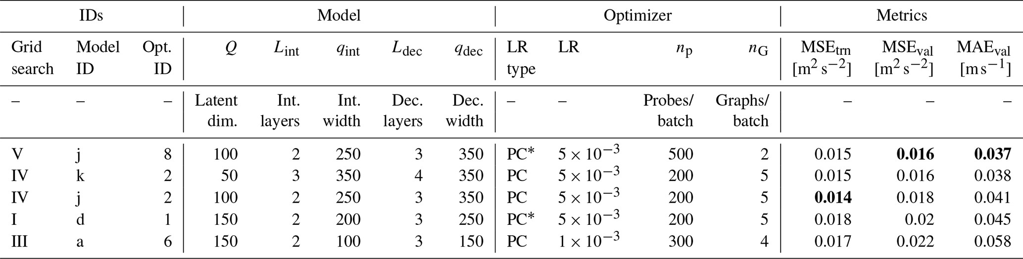
(PC) Piecewise constant. ^† LR schedule not triggered during training.

For the interested reader, details of the parameters considered during the grid search are reported in Appendix D. Table D1 lists the considered model and optimizer configurations; each model configuration is assigned a letter ID, and each optimizer configuration is assigned a numeric ID. The different combinations were trained, and the results are presented in Table D2. This includes the model and optimizer IDs, a grid search number in roman numerals, the training loss (MSE_trn), and two validation metrics (MSE_val and MAE_val). Entries are ranked by MSE_val, as this serves as the selection criterion for the best overall model.

The best five models from the hyperparameter search are presented in Table 1; the best combination was Vj8, which featured the largest considered decoder, with the remaining parameters in the middle of the explored ranges.

The best-performing models in Table 1 show a high correlation between MSE_val and MAE_val. Since these metrics weigh errors differently, this increases confidence that the model selection is robust and not overly sensitive to the choice of metric.

Table 2 Test set error metrics for the five best-performing models based on the grid search and a no-wake baseline, with the best metrics marked in bold. The naive baseline predicts that the flow everywhere is equal to the free-stream velocity (i.e., $u^{\prime }=U$).

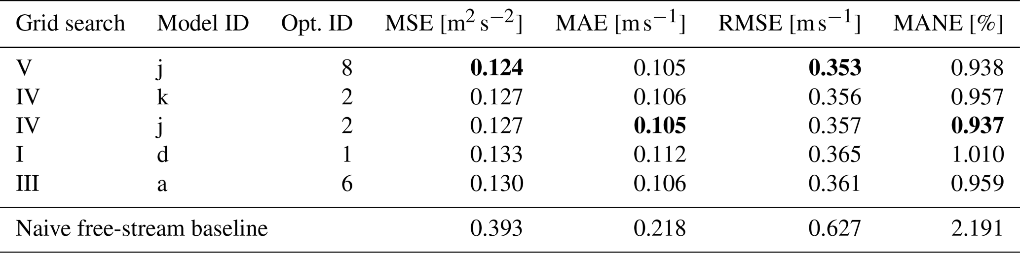
Based on the grid search, the five best-performing models by MSE_val have been evaluated on the unseen and unscaled test set using the metrics in Eq. (14); the results are reported in Table 2. Unlike the training and validation metrics used to compare models, the test metrics also include the more interpretable RMSE and MANE. Additionally, a naive baseline has been created, assuming no wake losses.

All five models perform similarly, indicating that, for the considered parameters, a minimum has been reached and that more substantial model changes are necessary to further improve performance. While the top model Vj8 from the grid search maintains the best score in terms of MSE and RMSE, it is the third-best model that achieves the best MAE and MANE. Interestingly, these two models share the same model configuration j but differ in the optimizer configuration, with the variation arising from the input configurations of n_p and n_G. This could indicate that the input configuration is less important than the model configuration. The number of message-passing steps (M) was fixed at 3 throughout the grid search, rather than treated as a tunable hyperparameter. Initial testing on a simpler model showed low sensitivity to additional message-passing steps, suggesting diminishing returns beyond M=3. While increasing M could theoretically improve performance in densely clustered farm configurations by propagating wake interactions across more neighbors, preliminary experiments did not support this hypothesis. However, the optimal value of M is suspected to be data dependent; higher-fidelity datasets capturing more complex wake dynamics or turbulence interactions may benefit from additional message-passing steps to fully resolve inter-turbine dependencies. A systematic sensitivity study on M across diverse farm configurations and data fidelities should be considered for future work.

3.2 Model performance

In this section, the performance of the best model from Table D2 is investigated. The testing is conducted in steps initially, where a random selection of each layout type is used to illustrate the model capabilities in the far wake at different downstream distances $\stackrel{\mathrm{̃}}{x}$ (see Fig. 3 for the definition of $\stackrel{\mathrm{̃}}{x}$). In the second step, a more data-centric approach is taken by illustrating the error statistics using the test set and analyzing the error with relation to different input types. Then, the model computational cost in terms of speed and memory is assessed, while varying the number of probe nodes to see the impact of graph size on computational cost.

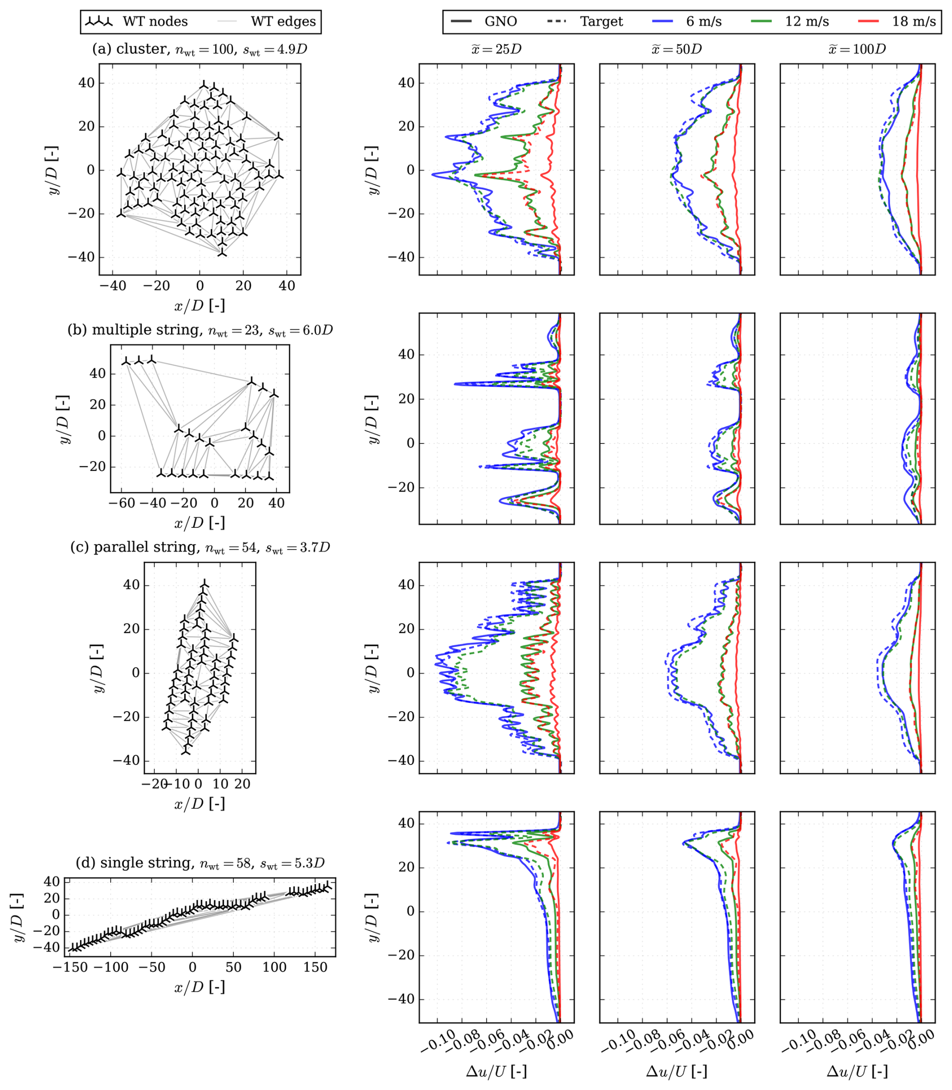
Figure 8 Normalized velocity deficit predictions and targets at different wind farm downstream distances $\stackrel{\mathrm{̃}}{x}\in \mathit{\{}\mathrm{25}D,\mathrm{50}D,\mathrm{100}D\mathit{\}}$ at I₀ = 5 %. (a) Cluster, (b) single string, (c) multiple string, and (d) parallel string.

3.2.1 Predictions

In Fig. 8a–d, velocity deficit (Δu) predictions made with the GNO are compared to the PyWake test data for a random layout of each layout type. The predictions are illustrated for three downstream distances $\stackrel{\mathrm{̃}}{x}=\mathit{\{}\mathrm{25},\mathrm{50},\mathrm{100}\mathit{\}}D$, at three free-stream wind speeds $U=\mathit{\{}\mathrm{6},\mathrm{12},\mathrm{18}\mathit{\}}$ m s⁻¹ and I₀ = 5 %. Unsurprisingly, the cluster farm with a number of wind turbines, n_wt=100, has the most significant wake effect but also the most smeared wake deficit, especially visible for the U = 6 m s⁻¹ scenario. The remaining layouts have fewer wind turbines but also more structured layouts. They show clearer peaks and valleys, especially the single-string layout. While the performance at U = 6 m s⁻¹ is satisfactory for all layouts, it becomes less accurate at higher wind speeds. At U = 12 m s⁻¹, the model performs the worst, although it captures the shape of the velocity deficit; the scale could be improved. In Fig. 8, the maximum velocity deficit error relative to $\widehat{u}$ ranges from 0.23 % to 6.13 % across the different inflow velocities and layouts.

Figure 9 Maximum absolute errors at each wind turbine for $\mathit{U}=[\mathrm{6},\mathrm{12},\mathrm{18}{]}^{\top }$ m s⁻¹ and I₀ = 5 %.

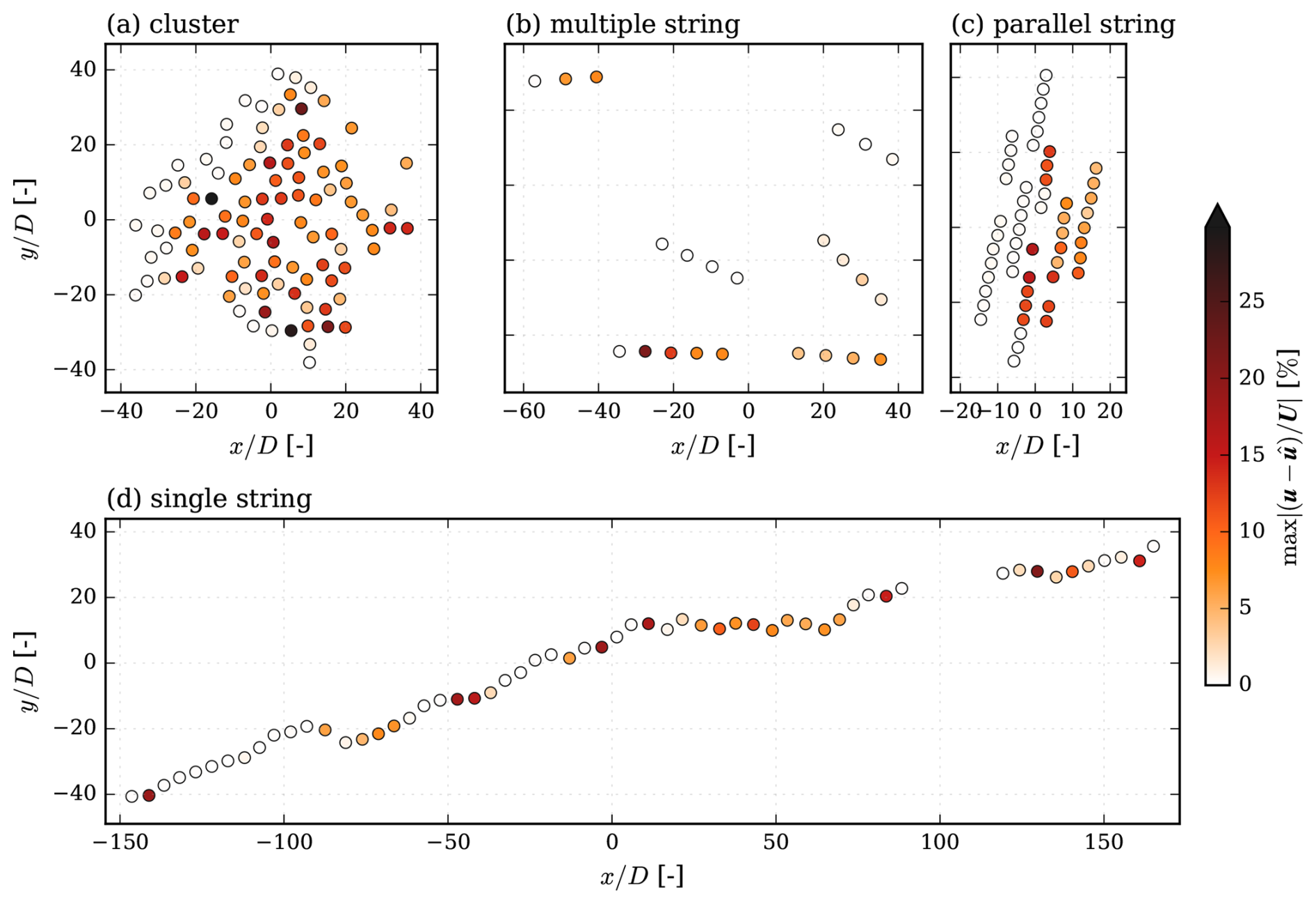
As a secondary output, the model can predict the velocity at individual turbines. To illustrate this capability, Fig. 9 shows the maximum error observed at each turbine for the same layouts and inflow velocities as those presented in Fig. 8, and the inflow direction is from left to right along the downstream direction x. In Fig. 9, it can be seen that waked turbines tend to have the largest errors. In Fig. 9c, the most significant error occurs where the density is high and the wake effect is substantial, while in Fig. 9a and d it can be seen that the turbines downstream of multiple others produce high errors, although the highest error occurs in the middle of a row. Figure 9b is of the type multiple string and happens to be a good example of the impact of string alignment with respect to the incoming wind having a significant effect on the errors. Here, the largest error occurs at the second turbine in a string aligned with the flow; this is most likely due to the induction effects playing a larger role. In general, where the wake effects are not as pronounced, the errors are smaller. For the interested reader, the relative absolute errors are also reported for individual wind speeds in Appendix E.

While several GNN-based models have been proposed for predicting quantities at turbine locations, a direct quantitative comparison is not feasible due to fundamental differences in farm configurations, prediction targets, training data sources, and evaluation metrics across studies. This is further complicated by the fact that detailed turbine-level error analysis has not been a primary focus in these works. For instance, Park and Park (2019) and Li et al. (2024) predict farm-level power, Ødegaard Bentsen et al. (2022) predict individual turbine power using a GAT, and Duthé et al. (2024) and de Santos et al. (2024) predict both loads and power. Furthermore, these models are specifically designed and optimized for turbine-level quantities, whereas predicting at turbine locations is not the primary objective of the GNO. Consequently, error characteristics should be viewed in the context of a model whose main purpose is to predict a spatially continuous flow field. Despite this, the GNO captures overall trends in turbine velocities well, suggesting that the learned flow representation encodes physically meaningful turbine interactions.

3.2.2 IEA Wind 740-10-MW reference wind farm

The reference wind farm consists of two layouts: a regular and an irregular layout as described in Sect. 2.4. For each layout, the total farm power output at each wind direction is computed and visualized using a polar grid. As the GNO does not inherently account for wind direction, this is achieved by translating and rotating the wind farm layout. In this way, each wind direction is represented as an equivalent new configuration. Repeating this process across all directions enables the calculation of wind-direction-dependent farm power, without requiring the model to explicitly encode directional information. This approach is feasible because the GNO has been trained on a large and diverse dataset comprising numerous wind farm configurations. Consequently, it generalizes well across a wide range of geometric arrangements and inflow conditions. The wind-direction-dependent farm power for a turbulence intensity of I₀ = 5 % is presented in Fig. 10.

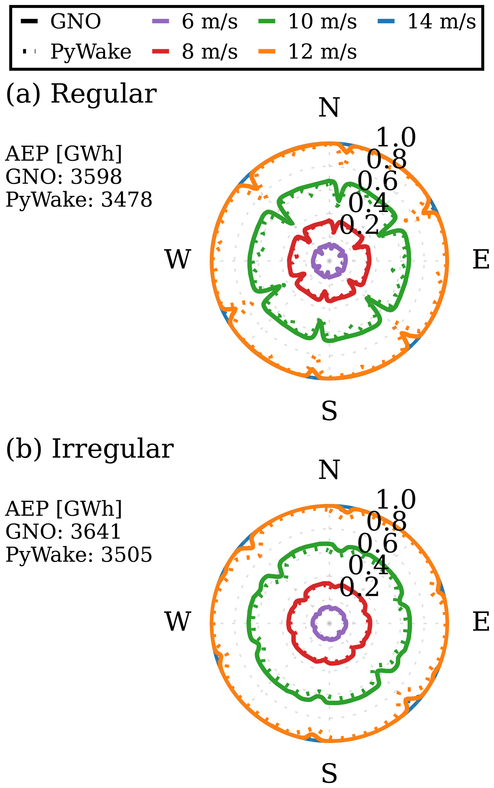
Figure 10 Normalized power production at different wind speeds and I₀ = 5 %, illustrated as power roses for the IEA Wind 740–10 MW reference wind farm (Kainz et al., 2024). (a) Regular layout pre-optimization and (b) irregular optimized layout.

As shown in Fig. 10a, the regular grid layout being non-optimized exhibits more pronounced internal wake effects and therefore produces lower overall power. In contrast, the irregular layout in Fig. 10b shows reduced wake interactions and higher power production across most wind directions. This result reflects the optimized nature of the irregular layout, which minimizes wake losses and enhances overall farm performance. In Fig. 10, an annual energy production (AEP) measure has been provided for each layout. It was found that the GNO consistently overestimates AEP by approximately 3.4 % and 3.9 % for the regular and irregular layouts, respectively. This is attributed to the tendency of the GNO to slightly underpredict wake deficits, leading to higher predicted turbine wind speeds and, consequently, inflated power estimates. Notably, the relative difference in AEP between the two layouts is well captured (the GNO predicts a 1.2 % increase from the regular to the irregular layout, compared to 0.8 % for PyWake), suggesting that the model can distinguish between layouts despite the absolute bias. Reducing this systematic offset, for instance, through improved training strategies or architectural refinements, should be considered for applications that require accurate absolute AEP estimates.

The GNO reproduces the overall power trends well for both layouts, with slightly improved accuracy for the irregular configuration. This behavior is consistent with previous observations that data-driven models tend to perform best under conditions similar to their training data and where variability is lower. The procedurally generated training layouts do not include simple regular grid configurations, which may explain the slightly lower accuracy on the regular IEA layout. Including such layouts in future datasets could improve generalization to such farms.

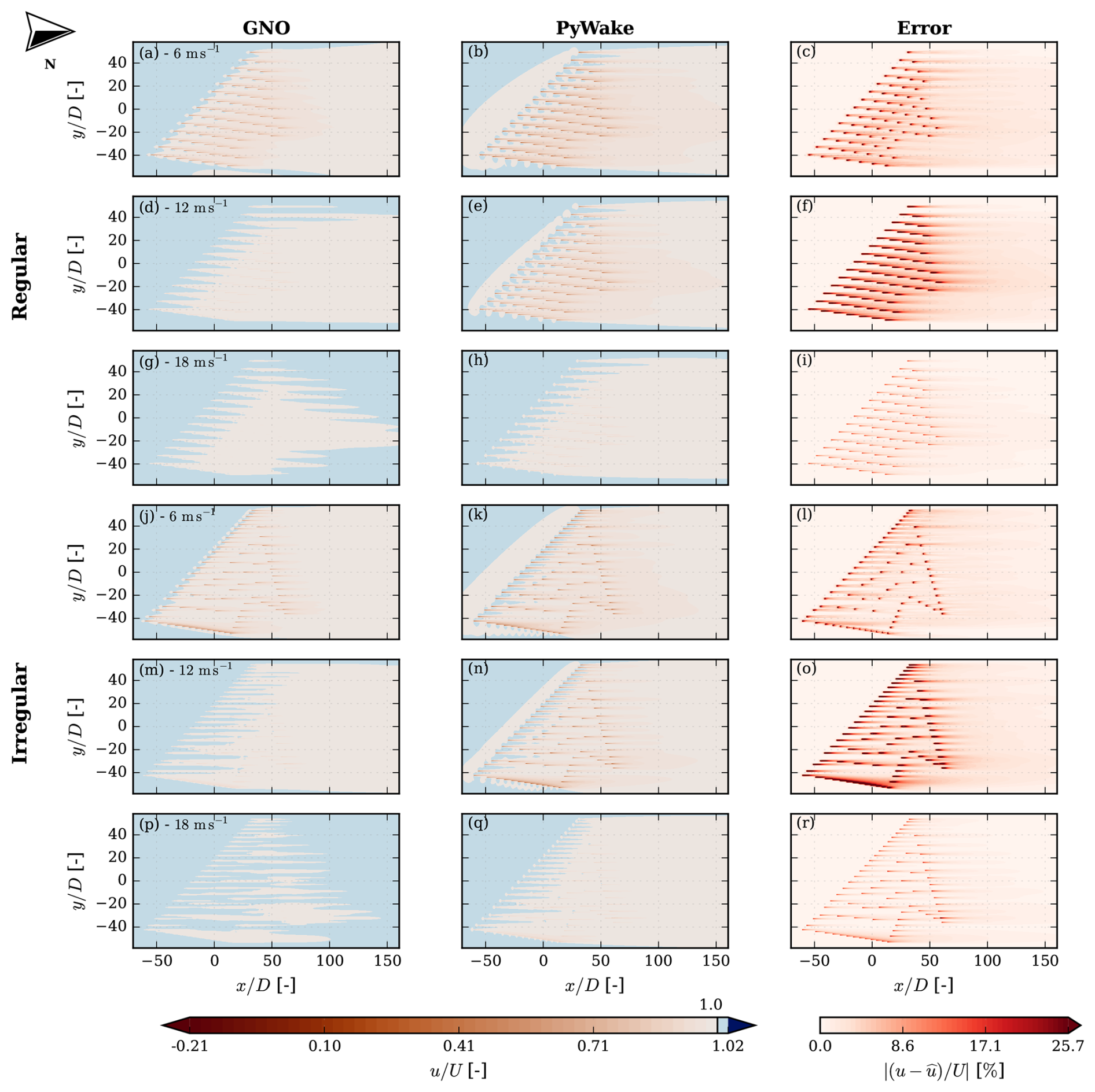
Figure 11 Contour plots depicting the flow around the IEA740 reference wind farm with columns depicting the GNO predicted output, the engineering model target output, and the error between the predictions for $\mathit{U}=[\mathrm{6},\mathrm{12},\mathrm{18}{]}^{\top }$ m s⁻¹ and I₀ = 5 %, rotated to the equivalency of incoming wind from the west.

At a wind speed of 14 m s⁻¹, both farms operate close to rated power, leading to small differences in predicted output. Some discrepancies remain at lower wind speeds and for specific wind directions where wake effects are more pronounced. The GNO successfully identifies the regions of strongest wake interaction, although the scale of the effects is not reproduced exactly. The model has been trained on data from within the farm and the far wake, but it does not perform well near the turbines. To demonstrate this model limitation, Fig. 11 shows predictions made with the GNO model, the PyWake targets, and their relative errors. Similar to the previous errors, we have seen that the largest errors are observed for U = 12 m s⁻¹, while errors are significantly smaller for both U = 6 m s⁻¹ and U = 18 m s⁻¹. The largest errors are consequently observed almost on top of the turbines, which is also where the largest and sometimes non-physical deficits are found.

The predictions made in Fig. 11 show promise but demonstrate that the model will need further improvements before it is ready for inter-farm flow simulations.

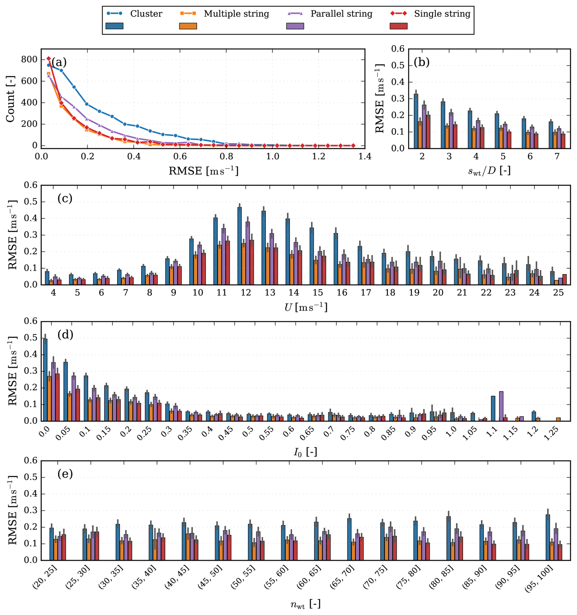
Figure 12 RMSE metrics for different layout types. (a) RMSE binned error counts. Binned RMSE (b) with respect to the separation factor s_wt, (c) at different free-stream velocities U, (d) across different TI, and (e) against the number of wind turbines n_wt.

3.2.3 Performance analysis

To evaluate the performance of the model under different scenarios, predictions are made for all combinations of layouts and inflows in the test dataset. For each layout, 10 000 probes are selected at equal spacings, and an RMSE is calculated for each flow case. The resultant metrics are displayed in Fig. 12, with separate visualizations for each layout type.

In Fig. 12a, binned counts of the RMSE metrics are illustrated for each layout type. The distributions show that the single- and multiple-string layouts have comparable distributions as the two lines lie almost on top of each other; they are simultaneously the best-performing layouts. The worst-performing layout type is the cluster, followed by the parallel string. To further investigate why that is the case, in Fig. 12b–e, bar plots of the errors are provided to investigate the effect of different aspects of the model inputs. Figure 12c shows a bar plot of the mean RMSE for different inflow wind speeds U. The four layouts share similar distributions with regard to U, all of them exhibiting the largest mean RMSE at U = 12 m s⁻¹. The largest error occurring at U = 12 m s⁻¹ is most likely related to the wind turbine C_T curve, as 12 m s⁻¹ is just past the steepest part of the curve in region III (see Fig. 2). This means that as turbines are affected by wakes inside the farm, the highest variability of C_T occurs at 12 m s⁻¹. Additionally, it is near the discontinuity of C_T when the rated wind speed is reached. To alleviate this, it is suggested that future implementations should rebalance the training dataset to proportionally include more flow cases right above the rated wind speed.

Figure 12d shows a bar plot of the mean RMSE as a function of ambient TI. As expected, there is an inverse correlation between RMSE and I₀. Lower I₀ indicates stronger wake effects, as the wake structure persists for longer, leading to a more complex farm flow and, consequently, higher errors. This occurs because turbulence breaks down wake structures and re-energizes the wind. At higher I₀ values, the RMSE increases again but so do the associated error bars. At the highest I₀ levels, a few extreme cases have no error bars, as there is only a single sample and therefore no spread. The sparsity of high I₀ values arises because the inflow cases were sampled to reflect realistic operating conditions rather than an even distribution of inflows. This is evident in Fig. 1g and h, where these extreme I₀ values are shown to be rare. Consequently, the limited number of samples for extreme I₀ values leads to the model being insufficiently trained for such scenarios, resulting in rising RMSE at the highest I₀ values. However, it is worth noting that these high TIs only occur at very low wind speeds and are extremely rare in the real world.

In Fig. 12b and e, the impact of the variables that govern the layout are investigated. These are the separation factor (s_wt) and the number of wind turbines (n_wt). All the layouts are strongly inversely correlated with s_wt. The cluster and the parallel string layouts do show a slight correlation to n_wt, but that is not the case for either the single-string or the multiple-string layout types.

In summary, there is a strong correlation between the model accuracy, the inflow condition and the separation of the turbines. Farms with fewer turbines and simpler wake interactions exhibit higher model accuracy, whereas larger dense farms show greater errors due to increasingly complex and nonlinear inter-turbine interactions. The configuration of the farm influences this behavior: layouts with wider turbine spacings promote simpler flow patterns, while denser configurations, such as cluster and parallel string layouts, intensify wake interactions and adversely affect the GNO predictive capability.

3.2.4 RBF kernels

One of the more interpretable trained parameters is the RBF kernels used to encode distances. While they do not tell the whole story – because MLPs are also used to encode features further – they do offer an indication of what is important. Figure 13a and b shows both the initial and final RBF kernels for the Vj8 model. Details of the kernel centers and widths are displayed in Fig. 13c and d. Overall, we can see that the widths are almost kept constant, while the centers have been shifted. The RBF kernels have moved closer together in two clusters, and the kernel originally in the middle has joined the cluster to the left of the center. In our formulation, the distance between a turbine receiving from an upstream-sending turbine becomes negative, as shown in Eq. (5). Since the wake effect is generally more important than the blockage, it makes sense that the training has prioritized five kernels in the negative direction and four in the positive.

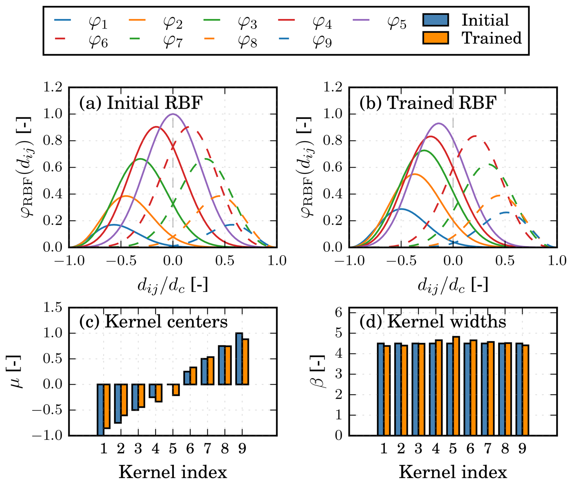
Figure 13 RBF kernels (a) before and (b) after training, with (c) kernel centers μ and (d) kernel widths β shown before and after training.

Computational cost and memory consumption

For a surrogate model, it is important to understand the computational cost associated with its execution, as it should be faster than the actual model it replaces. As previously mentioned, the implementation is based on Jax, which enables Just-In-Time (JIT) compilation, making the GNO suitable for scenarios requiring multiple evaluations. For completeness, the GNO is evaluated in three configurations: (i) a pre-JIT-compiled state, which most closely reflects the intended real-world application; (ii) without JIT compilation; and (iii) with JIT compilation but performing only a single prediction. To encompass a wide range of graph sizes, the whole test set is used with a variable number of probe nodes: $n_{\mathrm{p}}\in \mathit{\{}\mathrm{1},\mathrm{10},\mathrm{100}\mathit{\}}\cup \mathit{\{}\mathrm{1000},\mathrm{2000},\mathrm{\dots },\mathrm{10}\mathrm{000}\mathit{\}}$.

The timings are compared against PyWake, where the number of probes is interpreted as the number of grid points in a flow map. All experiments are conducted using CPU resources for comparability, as PyWake does not currently support GPU acceleration. Timing results are reported in CPU hours (CPUh), as PyWake can be executed on a single CPU core, whereas the surrogate model defaults to utilizing all available 32 cores. The CPU is not saturated for small and moderate graph sizes, putting the surrogate at a slight disadvantage. The results of this analysis are presented in Fig. 14. Figure 14a shows the overall timings, illustrating how costly it is to run the model without compilation and highlighting the significant upfront cost associated with compiling it. Once compiled, the results indicate that the computational cost of running the model increases with the graph size $\left|G\right|$ and that a performance improvement of approximately ∼ 10× can be expected compared to PyWake.

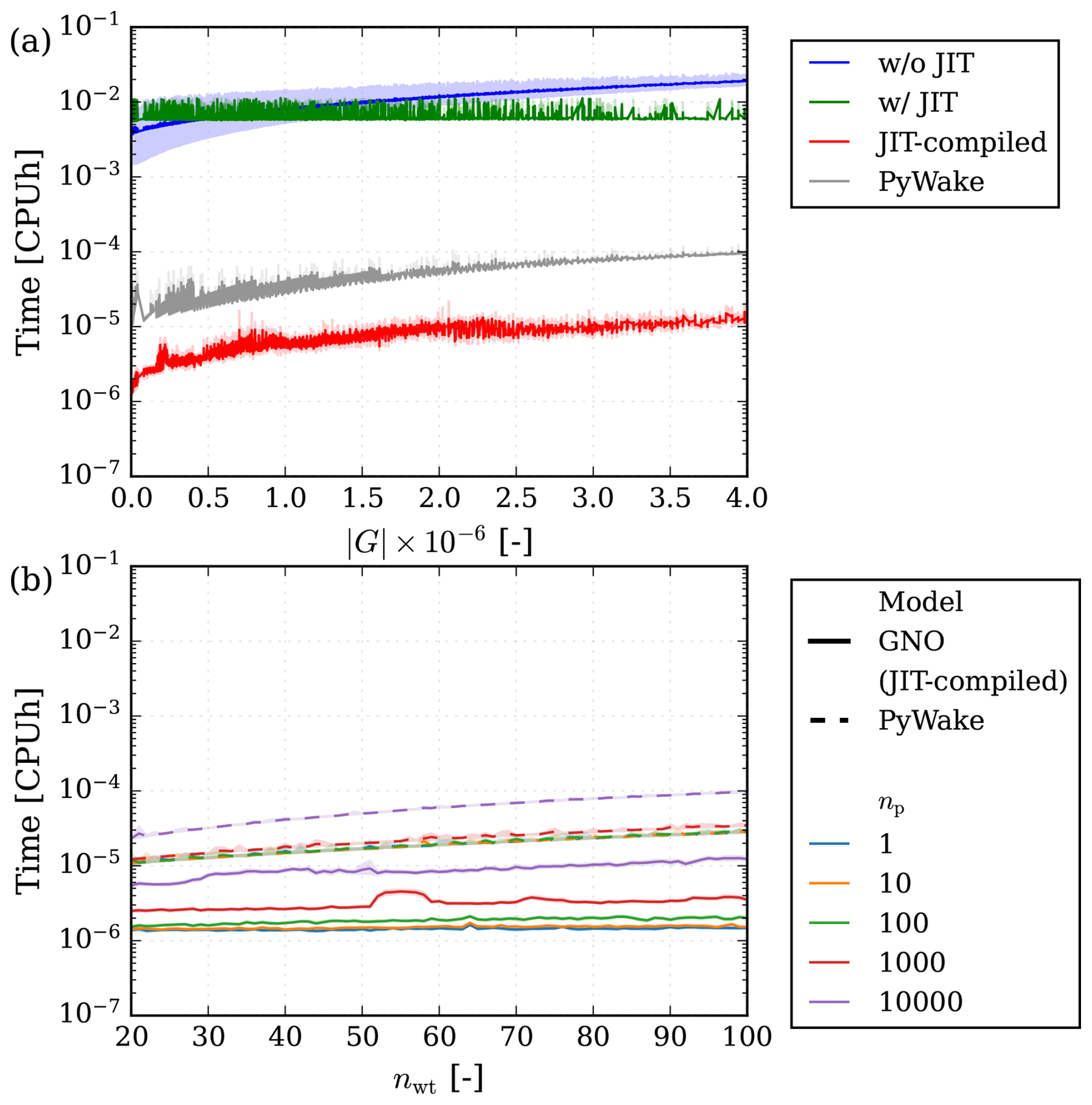
Figure 14 Model computational cost in terms of CPU hours. (a) Model cost of GNO in different JIT states compared to PyWake for varying graph sizes $\left|G\right|$. (b) Model computational cost in JIT-compiled state shown with different numbers of probes compared to PyWake for an increasing number of wind turbines.

To further investigate the GNO, each component described in Sect. 2.3 was timed independently. The timings were measured both (i) in a pre-JIT-compiled state and (ii) after JIT compilation. The results are shown in Fig. 15. The results show that, at larger graph sizes, prediction time is dominated by the encoding stage. In Fig. 15a, the computational cost increases almost linearly on the logarithmic axis, implying exponential growth in computational cost. This behavior is partly due to how the graphs were scaled by simply adding a large number of probes, which causes $\left|N_{\mathrm{p}}\right|$ and $\left|E_{\mathrm{p}}\right|$ to grow rapidly, while $\left|N_{\text{wt}}\right|$ and $\left|E_{\text{wt}}\right|$ remain unchanged. Consequently, the wind turbine interactions at the approximator stage are unaffected. Batching graphs is proposed for a more comprehensive analysis but has not been investigated further.

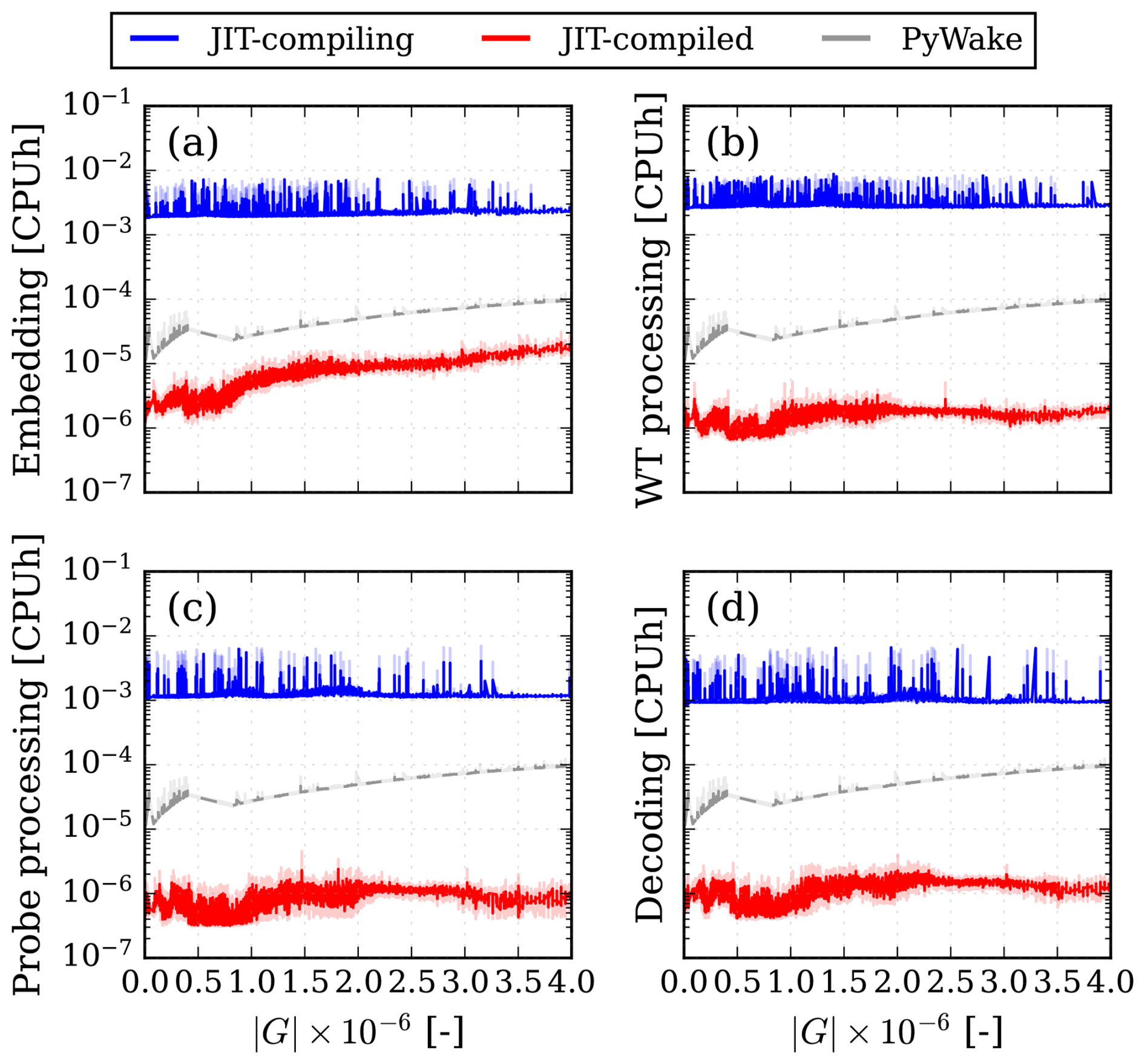
Figure 15 Timings of the GNO components. (a) Encoder ℰ, (b) approximator 𝒜, (c) decoder 𝒟 part 1: probe processing, and (d) decoder 𝒟 part 2: node decoding.

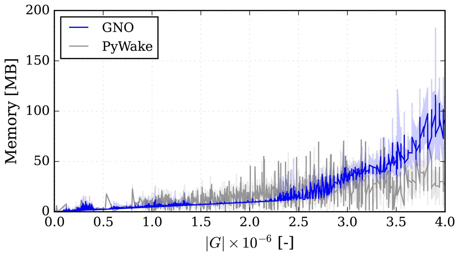
In Fig. 16, the memory consumption of the GNO is compared to the PyWake examples. As can be seen, there is no significant difference in consumed memory. However, at larger graph sizes, the memory consumption of the GNO starts growing more rapidly and, in some cases, overtakes the memory consumption of PyWake.

Figure 16 Memory consumption.

In summary, the GNO produces meaningful results that reflect the behavior of the flow around a given wind farm. As seen in Fig. 8, the accuracy increases with the distance behind the farm ($\stackrel{\mathrm{̃}}{x}$). Therefore, a suitable application could be the assessment of long-distance wakes from neighboring farms, e.g., during WFLO. The GNO is particularly well-suited for this purpose, as the model is highly adaptable with respect to layout configurations. The two-stage structure of the GNO means a neighboring farm only needs to be encoded once, and the resulting latent turbine states can then be reused to evaluate wake deficits at any query location. In practice, this allows candidate turbine positions to be assessed without reprocessing the neighboring wind farm each time, saving computation when exploring many layout alternatives.

As a surrogate for engineering models, the GNO was found to predict ∼ 10 times faster than PyWake. While this is an acceptable improvement, the speed-up would increase significantly if a higher-fidelity model were to be used as the basis. For example, if RANS were considered, a speed-up between 10⁴ and 10⁵ seems realistic given the relative cost difference between RANS and engineering models (van der Laan et al., 2015).

4 Conclusions

The GNO offers a new perspective on data-driven wind farm flow modeling. It has been established as a novel approach inspired by classic engineering models, demonstrating how the superposition principle can be integrated directly into the learning process, rather than relying on algebraic wake superposition as single-wake surrogate models require. Furthermore, the scalability and versatility of the graph-based approach have been shown to hold across highly varied layouts and inflow conditions, indicating that the model can perform well in a general sense.

The GNO was evaluated, and the results show that the model compares favorably in terms of computational cost and performs on par with PyWake for memory consumption. The model was found to evaluate with a computational cost of between 10⁻⁶ and 10⁻⁵ CPUh, equivalent to 3.6–36 ms on a single core, which is well within an acceptable range for practical applications. The GNO does not fully reproduce the PyWake data, which is unsurprising given that a surrogate will inevitably introduce some approximation error relative to its source model. Nevertheless, the accuracy of the GNO remains reasonably high when evaluated on a previously unseen test dataset. An overall RMSE of 0.353 ms⁻¹ and a MANE of 0.938 % were obtained. While these values constitute an acceptable error level, they do not provide the complete picture.

To gain deeper insight into the model performance, a more fine-grained assessment was conducted. First, the prediction error for representative cases was examined. This analysis demonstrated that the model accurately captures the wake shape, although some deviations persist in the predicted magnitude at medium wind speeds. A more comprehensive performance analysis revealed that the GNO performs best in scenarios with limited wake interactions. This trend is observed under inflow conditions with high TI, as well as at both low and high wind speeds. In contrast, performance deteriorates at medium wind speeds in the early part of turbine region III, where the high variability of C_T introduces additional complexity. Similarly, layouts with high turbine density, corresponding to a low separation factor, also result in reduced model accuracy. The impact of the total number of turbines was less pronounced, but a slight preference for smaller farms was observed for the cluster and parallel string layout types.

The GNO presented in this work represents a methodological contribution to data-driven wind farm modeling. Nonetheless, several areas for improvement remain. Therefore, some suggestions are made for further work. The current dataset was created using engineering models, which, by design, apply a linear summation of wakes. Even though the All2AllIterative scheme introduces nonlinear interactions between turbines, it still merges wakes linearly. The next logical step is to utilize higher-fidelity training data that incorporates turbine interactions directly into the model. The most suitable choice would likely be RANS, as its computational cost is significantly lower than that of other computational fluid dynamics (CFD) methods. To further reduce costs, a transfer-learning scheme could be introduced that combines engineering models with RANS, similar to the approach of Duthé et al. (2024). The current GNO exclusively uses a GEN core, which, combined with Softmax aggregation, provides only a rudimentary attention mechanism. However, more powerful attention mechanisms exist in both GAT and full transformer-based attention layers. Incorporating either of these into the wind turbine processing or probe processing steps could allow the model to approximate a more complex operator. A mixed-modeling approach could also be developed, incorporating PyWake as an additional approximator alongside the GNO to predict a higher-fidelity flow field, thereby forming a multi-fidelity upscaling framework. Integrating this with a more advanced attention mechanism could enable the formation of more physically meaningful graph connections. Although such an approach would likely be more computationally expensive than the model proposed in this work, it would serve as a CFD surrogate and thus remain comparatively affordable. Furthermore, the current decoder architecture processes probe nodes in a single step without probe-to-probe communication. Introducing multiple message-passing steps between probe nodes could enable the model to capture finer spatial correlations in the flow field. However, to be meaningful, this extension would require higher-fidelity training data.

Overall, the GNO presented in this work provides a baseline for efficient data-driven flow prediction in complex wind farm environments. Further improvements can be achieved by incorporating higher-fidelity training data, enhanced attention mechanisms, and multi-fidelity coupling strategies, thereby improving its predictive performance. As these developments are implemented, the GNO model is well positioned to become a valuable tool for both research and industrial applications.

Appendix A: Wind farm simulation implementation details

Additional details about the wind farm modeling set-up using PyWake are given in this appendix for interested readers.

For estimating the velocity deficit, the NiayifarGaussianDeficit by Niayifar and Porté-Agel (2016) is shown in Eq. (A1):

$$\begin{array}{}\text{(A1a)}& {\displaystyle }\begin{array}{rl}{\displaystyle \frac{\mathrm{\Delta }u}{U}}=& \left(\mathrm{1}-\sqrt{\mathrm{1}-{\displaystyle \frac{C_{\mathrm{T}}}{\mathrm{8}{\left({\displaystyle \frac{k^{\ast }x}{D+{\mathit{\epsilon }}_{\mathrm{d}}}}\right)}^{\mathrm{2}}}}}\right)\\ & \times \exp \left(-{\displaystyle \frac{\mathrm{1}}{\mathrm{2}{\left({\displaystyle \frac{k^{\ast }x}{D+{\mathit{\epsilon }}_{\mathrm{d}}}}\right)}^{\mathrm{2}}}}{\left({\displaystyle \frac{y}{D}}\right)}^{\mathrm{2}}\right)\end{array}\text{(A1b)}& {\displaystyle }{\mathit{\epsilon }}_{\mathrm{d}}=\mathrm{0.2}\sqrt{{\mathit{\beta }}_{\mathrm{d}}},{\mathit{\beta }}_{\mathrm{d}}={\displaystyle \frac{\mathrm{1}}{\mathrm{2}}}{\displaystyle \frac{\mathrm{1}+\sqrt{\mathrm{1}-C_{\mathrm{T}}}}{\sqrt{\mathrm{1}-C_{\mathrm{T}}}}},C_{\mathrm{T}}<\mathrm{0.9}\text{(A1c)}& {\displaystyle }{k}^{\ast }=a_{\mathrm{1}}{I}_{\text{wt}}+a_{\mathrm{2}},a_{\mathrm{1}}=\mathrm{0.3837},a_{\mathrm{2}}=\mathrm{0.003678},\end{array}$$

where x is the streamwise direction, Δu is the velocity deficit in the x direction, C_T is the coefficient of thrust, ε_d is a shape parameter offset dependent on C_T defined in Eq. (A1b), and a₁ and a₂ are experimentally fitted parameters derived with large-eddy simulation (LES) data.

The CrespoHernandez-added TI model by Crespo and Hernández (1996) depends on the induced velocity factor and the distance behind the turbine, as shown in Eq. (A2):

$$\begin{array}{}\text{(A2a)}& {\displaystyle }{I}_{\mathrm{a}}& {\displaystyle }=\mathrm{0.73}{a}_{\mathrm{m}}^{\mathrm{0.8325}}{I}_{\mathrm{0}}^{\mathrm{0.0325}}{\left({\displaystyle \frac{x}{D}}\right)}^{-\mathrm{0.32}}\text{(A2b)}& {\displaystyle }{a}_{\mathrm{m}}& {\displaystyle }=\mathrm{0.083}{C}_{\mathrm{T}}^{\mathrm{3}}+\mathrm{0.0586}{C}_{\mathrm{T}}^{\mathrm{2}}+\mathrm{0.2460}{C}_{\mathrm{T}},\end{array}$$

where a_m is the induced velocity factor estimated with an empirical polynomial fit of C_T to address cases with a_m≥0.5, as described by Madsen et al. (2020).

SelfSimilarityDeficit2020 by Troldborg and Meyer Forsting (2017) and Forsting et al. (2023) calculates the blockage deficit produced by individual wind turbines (Δu_b). It is based on the observation that inductions are radially self-similar for upstream distances greater than 1 rotor radius (R). It consists of an axial- and a radial-shaped function. The newer version of the model includes an updated linear induction zone half-radius ($r_{\mathrm{1}/\mathrm{2}}$), which corrects the behavior of turbine induction in wind farm contexts.

$$\begin{array}{ll}\text{(A3a)}& {\displaystyle }& {\displaystyle \frac{\mathrm{\Delta }{u}_{\mathrm{b}}}{U}}=a_{\mathrm{0}}(x,C_{\mathrm{T}})\mathit{\nu }\left(x\right){\text{sech}}^{\mathit{\alpha }}\left({\mathit{\beta }}_{\mathrm{b}}{\displaystyle \frac{r}{r_{\mathrm{1}/\mathrm{2}}\left(x\right)}}\right),\text{(A3b)}& {\displaystyle }& {\displaystyle }\mathit{\nu }\left(x\right)=\left(\mathrm{1}+{\displaystyle \frac{x/R}{\sqrt{\mathrm{1}+{\left(x/R\right)}^{\mathrm{2}}}}}\right),\text{(A3c)}& {\displaystyle }& {\displaystyle }{a}_{\mathrm{0}}(x,C_{\mathrm{T}})={\displaystyle \frac{\mathrm{1}}{\mathrm{2}}}\left(\mathrm{1}-\sqrt{\mathrm{1}-\mathit{\gamma }\left(x,C_{\mathrm{T}}\right)\cdot C_{\mathrm{T}}}\right),\text{(A3d)}& {\displaystyle }& {\displaystyle \frac{r_{\mathrm{1}/\mathrm{2}}\left(x\right)}{R}}=\mathit{\lambda }\cdot (x/R)+\mathit{\eta },{\displaystyle }& {\displaystyle }\mathit{\alpha }=\mathrm{8}/\mathrm{9}{\mathit{\beta }}_{\mathrm{b}}=\sqrt{\mathrm{2}}\mathit{\lambda }=-\mathrm{0.672},\mathit{\eta }=\mathrm{0.4897},\end{array}$$

where ν is the centerline induction and a₀ is the axial induction factor. The SelfSimilarityDeficit2020 model introduced a γ(x,C_T) function that gradually changes from a far-field expression to a near-field expression. Here, this is formulated as a function δ(x). The near- and far-field γ functions are parameterized with $\stackrel{\left(i\right)}{c_{\text{nf}}}$ for the near-field γ and $\stackrel{\left(i\right)}{c_{\text{ff}}}$ for the far-field γ.

$$\begin{array}{}\text{(A4a)}& {\displaystyle }\begin{array}{rl}& \mathit{\gamma }\left(x,C_{\mathrm{T}}\right)=\mathit{\left\{}\mathit{\delta }\right(x)\cdot \left(\stackrel{\left(\mathrm{1}\right)}{c_{\text{nf}}}\cdot \sin \left({\displaystyle \frac{C_{\mathrm{T}}+\stackrel{\left(\mathrm{2}\right)}{c_{\text{nf}}}}{\stackrel{\left(\mathrm{3}\right)}{c_{\text{nf}}}}}\right)+\stackrel{\left(\mathrm{4}\right)}{c_{\text{nf}}}\right)\\ & +(\mathrm{1}-\mathit{\delta }(x\left)\right)\cdot \left(C_{\mathrm{T}}^{\mathrm{3}}\stackrel{\left(\mathrm{1}\right)}{c_{\text{ff}}}+C_{\mathrm{T}}^{\mathrm{2}}\stackrel{\left(\mathrm{2}\right)}{c_{\text{ff}}}+C_{\mathrm{T}}\stackrel{\left(\mathrm{3}\right)}{c_{\text{ff}}}+\stackrel{\left(\mathrm{4}\right)}{c_{\text{ff}}}\right)\mathit{\}}\end{array}\text{(A4b)}& {\displaystyle }\begin{array}{rl}& \stackrel{\left(\mathrm{1}\right)}{c_{\text{nf}}}=-\mathrm{1.381},\stackrel{\left(\mathrm{2}\right)}{c_{\text{nf}}}=\mathrm{2.627},\\ & \stackrel{\left(\mathrm{3}\right)}{c_{\text{nf}}}=-\mathrm{1.524},\stackrel{\left(\mathrm{4}\right)}{c_{\text{nf}}}=\mathrm{1.336},\\ & \stackrel{\left(\mathrm{1}\right)}{c_{\text{ff}}}=-\mathrm{0.06489},\stackrel{\left(\mathrm{2}\right)}{c_{\text{ff}}}=-\mathrm{0.4911},\\ & \stackrel{\left(\mathrm{3}\right)}{c_{\text{ff}}}=-\mathrm{0.1577},\stackrel{\left(\mathrm{4}\right)}{c_{\text{ff}}}=\mathrm{1.116},\end{array}\text{(A4c)}& {\displaystyle }\mathit{\delta }\left(x\right)=\left\{\begin{array}{ll}\mathrm{1}& \text{for }x/R<-\mathrm{6}\\ {\displaystyle \frac{\left|\mathit{\nu }\left(x\right)-\mathit{\nu }\right|}{\mathit{\nu }(-\mathrm{6})-\mathit{\nu }(-\mathrm{1})}}& \text{for }-\mathrm{6}\le x/R\le -\mathrm{1}\\ \mathrm{0}& \text{for }-\mathrm{1}<x/R\end{array}\right.\end{array}$$

Appendix B: Neural network components

Dropout

Our version of dropout uses inverse probability scaling, so the entire dropout layer can be ignored during inference. During training, dropout is applied after both Eqs. (7a) and (7b):

$$\begin{array}{}\text{(B1a)}& {\displaystyle }{z}_{\mathrm{j}}^{\left(l\right)}& {\displaystyle }\sim \text{Bernoulli}\left(P_{\mathrm{D}}\right),j=\mathrm{1},\mathrm{2},\mathrm{\dots },N_{\mathrm{a}}\text{(B1b)}& {\displaystyle }{\stackrel{\mathrm{̃}}{\mathit{\xi }}}^{\left(l\right)}& {\displaystyle }={\mathit{z}}^{\left(l\right)}\odot {\displaystyle \frac{\mathrm{1}}{\mathrm{1}-P_{\mathrm{D}}}}\cdot {\mathit{\xi }}^{\left(l\right)},l=\mathrm{1},\mathrm{2},\mathrm{\dots },L.\end{array}$$

Here, z^(l) is a dropout mask consisting of zeros and ones, created with Bernoulli(P_D) (the Bernoulli distribution given the dropout probability (P_D)), N_a is the number of activations in layer l, the operator ⊙ denotes the Hadamard element-wise product, and ${\stackrel{\mathrm{̃}}{\mathit{\xi }}}^{\left(l\right)}$ is the resultant hidden state with dropout applied.

Layer normalization

The formulation of layer normalization used is shown in Eq. (B2):

$$\begin{array}{}\text{(B2a)}& {\displaystyle }{\mathit{\mu }}_{\text{LN}}^{\left(L\right)}={\displaystyle \frac{\mathrm{1}}{H}}\sum _{i=\mathrm{1}}^H{\mathit{\xi }}_{\mathrm{i}}^{\left(L\right)},{\mathit{\sigma }}_{\text{LN}}^{\left(L\right)}=\sqrt{{\displaystyle \frac{\mathrm{1}}{H}}\sum _{i=\mathrm{1}}^H{\left({\mathit{\xi }}_{\mathrm{i}}^{\left(L\right)}-{\mathit{\mu }}_{\text{LN}}^{\left(L\right)}\right)}^{\mathrm{2}}},\text{(B2b)}& {\displaystyle }{\stackrel{\mathrm{‾}}{\mathit{\xi }}}^{\left(L\right)}={\mathit{s}}_{\text{LN}}\odot {\displaystyle \frac{{\mathit{\xi }}^{\left(L\right)}-{\mathit{\mu }}_{\text{LN}}^{\left(L\right)}}{{\mathit{\sigma }}_{\text{LN}}^{\left(L\right)}+\mathit{\epsilon }}}+{\mathit{b}}_{\text{LN}},\end{array}$$

where ${\mathit{\mu }}_{\text{LN}}^{\left(L\right)}$ and ${\mathit{\sigma }}_{\text{LN}}^{\left(L\right)}$ denote the layer mean and standard deviation, ${\mathit{\xi }}_{\mathrm{i}}^{\left(L\right)}$ is the ith activation at the last MLP layer L, and ${\stackrel{\mathrm{‾}}{\mathit{\xi }}}^{\left(L\right)}$ represents the layer-normalized hidden states, while s_LN and b_LN are trainable scale and bias parameters, and $\mathit{\epsilon }=\mathrm{1}\times {\mathrm{10}}^{-\mathrm{6}}$ is added for numerical stability.

Appendix C: GNO data loading

As with other neural operators, the data comes in triplets: branch input (the wind farm graph encoding turbine positions and inflow conditions), trunk input (the probe graph encoding query locations), and target output. For a broader context, see, e.g., (Lu et al., 2021; Seidman et al., 2022). Because both the GNO branch and trunk are GNNs, the branch input is a graph, and the trunk is a second graph with a separate edge configuration. One of the core strengths of GNNs is the ability to process graphs of different sizes. However, to leverage the efficiency of the Jax framework, it is necessary to use JIT compilation, which requires inputs to have fixed sizes and shapes. To create graphs of fixed sizes and shapes, graphs are dynamically batched together until they reach a maximum size, defined by the number of graphs, total nodes, and total edges.

Batching graphs differ from conventional batching. In traditional batching, inputs share identical dimensions, and batching is performed along a new dimension. However, because the number of nodes and edges vary for each graph, batching is achieved by combining multiple graphs into a single larger graph. This approach preserves the sub-graph individual characteristics by ensuring no edges between sub-graphs, thus preventing interactions during training and inference. Dynamic batching involves adjusting the number of graphs in each batch to fit within the size constraints rather than using a fixed batch size as in conventional batching. When dynamic batching is employed, adding another graph to the batch is prohibited once any maximum size limit is reached, as doing so would violate the constraints. Instead, padding with empty graphs, edges, and nodes is used to meet the target size.

An additional challenge arises because Jax does not currently offer a native data loader. At the time of writing, the most popular and mature Python framework for GNNs is PyG. Consequently, the PyG data loader has been used to load data in parallel from the file system into memory. Afterward, the graphs are converted to the Jraph format. Finally, dynamic batching and padding are performed sequentially on the CPU before the data are transferred to the GPU for processing. The current performance bottleneck lies in the sequential dynamic batching process. Parallelizing this step is challenging due to the variable sizes of the graphs. However, this method is still significantly more efficient than loading data from the file system sequentially. The process is visualized in Fig. C1.

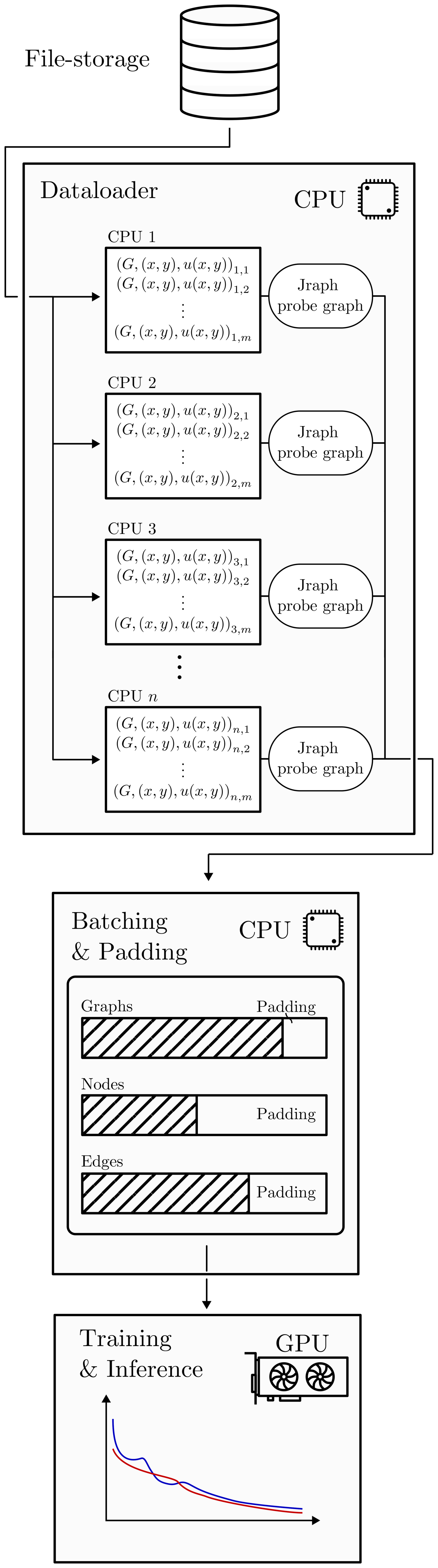
Figure C1 Flowchart diagram illustrating the steps from on-disk memory, constructing the Jraph compatible probe graph in parallel, batching, padding, and moving the resultant batched and padded probe graph to video memory.

Appendix D: Hyperparameter search detail

Table D1 Model and optimizer configurations used in the grid search.

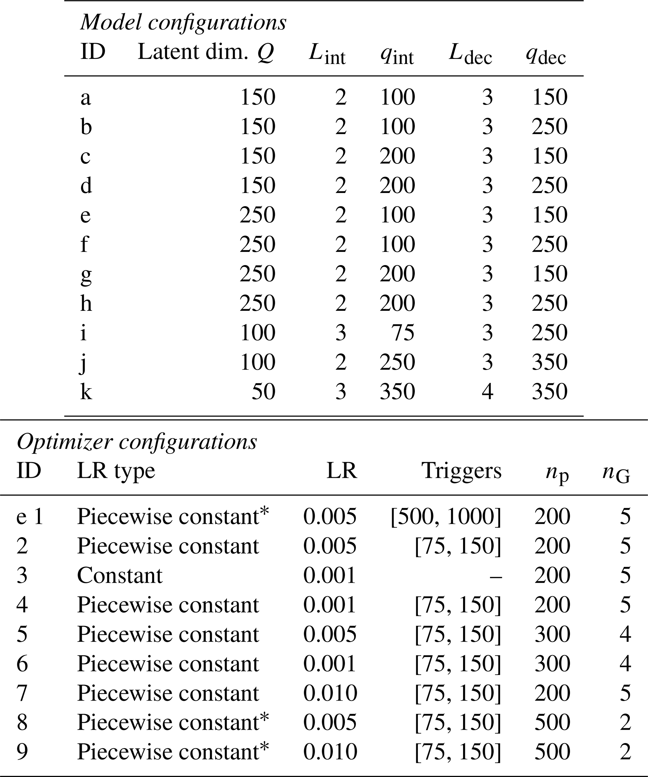
^∗ Learning rate schedule was not triggered during training.

Table D2 Trained models from the grid search, ranked by validation MSE_val. The best metric is marked in bold.

Appendix E: Wind turbine prediction visualization

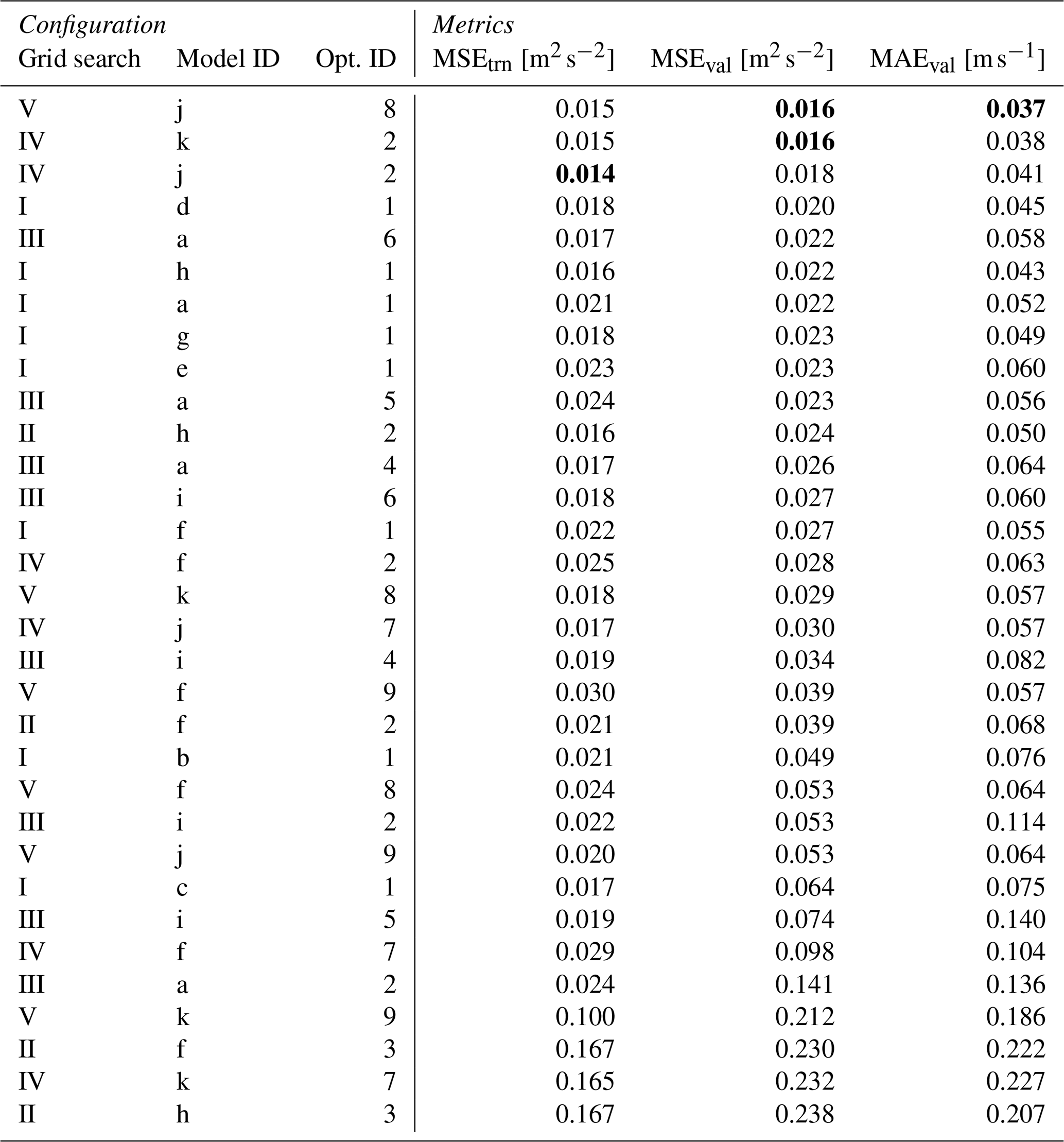
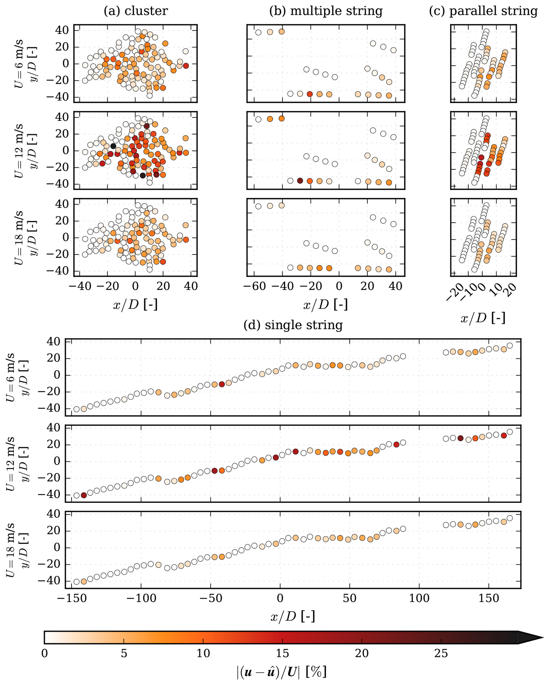
Figure E1 Maximum absolute errors at each wind turbine for each wind speed in $\mathit{U}=[\mathrm{6},\mathrm{12},\mathrm{18}{]}^{\top }$ m s⁻¹ and I₀ = 5 %.