A semi-empirical model for near-sea-surface wind speed deficits downstream of offshore wind parks in the German Bight fitted to satellite synthetic aperture radar measurements

A two-dimensional advection/diffusion model for the near-sea-surface wind speed deficit downstream of offshore wind parks is fitted to satellite synthetic aperture radar (SAR) data. The Wake2Sea model enables the inclusion of offshore wind farm (OWF) wake effects in existing atmospheric model data at low computational costs and employs the standard Fitch parameterisation to describe the momentum sink associated with wind turbines. Model wind fields from the German weather centre are used as prior information about the unperturbed atmosphere without OWFs. Using 30 Sentinel-1A/Sentinel-B satellite SAR scenes acquired over the German Bight representing different stability and wind speed regimes, a 4D-Var scheme is applied to optimise the agreement between simulated and observed radar cross sections. The method adjusts eight parameters in the wake model and also applies corrections to the background wind field on a spatial scale of 40 km. An L-curve analysis is applied to choose the weighting of prior knowledge and observations in the cost function. The method improves the match between observations and simulations significantly, if uncorrected model wind fields are used as a baseline. Furthermore, the inclusion of the empirical wake model leads to improvements when the background-corrected wind field is used as a reference. Comparisons with data measured at the fixed platform FINO-1 adjacent to the first German offshore wind park Alpha Ventus and with airborne campaign measurements showed that the proposed inclusion of wakes in the atmospheric model data leads to a significantly improved match.

1 Introduction

The global installed offshore wind energy power has increased about 10-fold over the last decade, reaching 64 GW in 2023 (WFO, 2023). With a share of about 47 %, China is currently the largest offshore wind farm (OWF) operator worldwide. Some studies suggest that over 380 GW of new offshore wind capacity will be added over the next decade globally (Williams and Zhao, 2023). In Europe, the United Kingdom is the country with the most installations, followed by Germany, with 14 and 8 GW installed power by 2023, respectively. According to the European Union (EU) Strategy on Offshore Renewable Energy, the installed offshore wind power in Europe will grow from about 28 GW in 2022 to about 60 GW by 2030 (European Commission, 2020). In Germany the goal to achieve 70 GW offshore wind energy by 2045 is written in law (Deutscher Bundestag, 2024).

It is obvious that these rapid developments come with a large spectrum of challenges in the economic, political and research sectors. A large number of studies that analyse the impact of offshore wind farms on the atmosphere already exist, often with a focus on wakes in the atmospheric boundary layer (ABL) (Siedersleben et al., 2020; Akhtar et al., 2021; von Brandis et al., 2023; Platis et al., 2018). One reason for this interest is the direct implications of these wakes for the optimisation of power yields considering shadowing effects, as well as the role of turbulent wakes in the fatigue loading of downstream turbines. The respective processes in the ABL have been studied with different types of numerical models, including mesoscale models (Siedersleben et al., 2020), large-eddy simulation (LES) models (Vollmer et al., 2017) and engineering models (Cañadillas et al., 2020). Furthermore, different types of observation techniques were applied, e.g. light detection and ranging (LIDAR) systems (Schneemann et al., 2020) and spaceborne synthetic aperture radar (SAR) sensors (Djath and Schulz-Stellenfleth, 2019). The existing studies show that OWF wakes can extend well above 100 km downstream in cases where the ABL is very stable. Typical wind speed deficits are in the range of 10 %–20 % (Djath et al., 2018). There is ongoing research about atmospheric wakes, e.g. concerning the interaction of wakes or the coupling with coastal effects (Djath et al., 2022; Schulz-Stellenfleth et al., 2022). Furthermore, there is still debate about optimal parameterisations of OWFs in numerical models (Fischereit et al., 2022; Ali et al., 2023).

In addition to the OWF effects in the ABL, potential impacts in the ocean have gained growing attention (Christensen et al., 2013; Broström, 2008; Christiansen et al., 2022; Daewel et al., 2022). Basically, two types of processes have been discussed in the literature so far:

• effects caused by the modified wind forcing at the sea surface (Christiansen et al., 2022; Daewel et al., 2022)

• effects related to the interaction of water with the OWF foundation structures (Christensen et al., 2013; Grashorn and Stanev, 2016; Carpenter et al., 2016; Carpenter and Guha, 2024).

The present study is connected to the modelling of the first type of processes, where accurate estimates of near-surface wind speeds in the surroundings of OWFs are required. A standard parameter used in both the ocean circulation and the ocean wave modelling communities is wind speed at 10 m height. As mentioned above, most studies concerned with OWF wakes in the ABL have focused on the impacts around the hub height, which are most relevant for power yields. Near-surface wind speeds around OWFs modelled with mesoscale models have been used to drive ocean models (Christensen et al., 2013), but very little has been done concerning the validation of these data. On the other hand, a large amount of satellite SAR data is available, which provide two-dimensional (2D) information on near-ocean-surface wind speeds with high spatial resolution (Lehner et al., 1998), but the condensation of this information on OWF wakes into a parameterised form is still at a very basic level (Djath et al., 2018; Christiansen et al., 2022). Against this backdrop, the main objectives of the present study are as follows:

• Condense the OWF wake information contained in SAR data into a 2D semi-empirical model, which captures the main characteristics but has small computational demands compared to a 3D atmospheric model.

• Design this model as a tool for ocean modellers to generate wind forcing for OWF impact studies, allowing for the consideration of a multitude of OWF scenarios not feasible with 3D atmospheric models.

The proposed semi-empirical model can be applied a posteriori to existing atmospheric model datasets to incorporate OWF wake effects. Many of these datasets, like ERA5 (Hersbach et al., 2020), are intensely used as references by the scientific community, and the proposed tool can massively enhance the applicability of these data for studying near-surface wake effects in the offshore wind farm context.

The proposed model, which is referred to as the Semi-empirical model for atmospheric offshore wind farm wakes near the sea surface (Wake2Sea) in the following, is based on the momentum conservation law and has a relatively simple functional form. It contains eight parameters, which were estimated using 30 SAR scenes covering a variety of different ABL stability and wind speed situations. It is shown that the model is capable of capturing major characteristics of OWF wakes like deficit intensity and wake length. A commonly used wind turbine parameterisation (Fitch parameterisations; Fitch et al., 2012) is used to include OWF properties, e.g. the thrust coefficient curve (C_T curve), in the model, and a dependence on ABL stability is contained in the formulation as well.

We would like to emphasise that the development of this model was guided by the requirements of the ocean community, i.e. the provision of wind information near the ocean surface. The current version of the model is not designed for the estimation of wind power at hub height. As expected, the model shows significantly smaller absolute wind speed deficits within wind farms for the 10 m near-surface wind compared to respective deficits at hub height computed with 3D atmospheric models.

The paper is structured as follows. In Sect. 2 the Wake2Sea model for wind speed deficits is introduced. Section 3 gives information about the atmospheric model and satellite data used in the study. The model inversion approach is described in Sect. 4. Results of the inversion, including comparisons with independent data measured at the FINO-1 platform and applications of Wake2Sea for the derivation of yearly deficit statistics, are presented in Sect. 5. Some theoretical analyses of the inversion results are described in Sect. 6, and conclusions are drawn in Sect. 7.

2 2D advection/diffusion model Wake2Sea for wind speed deficits

The semi-empirical wake model used in this study is based on a simplified form of the Navier–Stokes momentum conservation equation for a layer of thickness dZ of the atmosphere above the ocean surface (Frandsen et al., 2006). Neglecting the Coriolis force and assuming that the 2D divergence of the horizontal wind field $U=(u,v)$ is small, i.e. negligible vertical air motion, we have

$$\begin{array}{}\text{(1)}& {\displaystyle \frac{\partial U}{\partial t}}\approx -U\cdot \mathrm{\nabla }U+{\mathit{\nu }}_{\mathrm{V}}{\displaystyle \frac{{\partial }^{\mathrm{2}}U}{\partial z^{\mathrm{2}}}}+{\mathit{\nu }}_H({\displaystyle \frac{{\partial }^{\mathrm{2}}U}{\partial x^{\mathrm{2}}}}+{\displaystyle \frac{{\partial }^{\mathrm{2}}U}{\partial y^{\mathrm{2}}}})-\mathrm{\nabla }p,\end{array}$$

where the horizontal diffusion coefficient ν_H is assumed constant, ν_V is the vertical diffusion coefficient and p is pressure. All quantities have to be interpreted as averages of the layer dZ. The vertical diffusion term can be approximated as

$$\begin{array}{}\text{(2)}& \begin{array}{rl}{\mathit{\nu }}_{\mathrm{V}}{\displaystyle \frac{{\partial }^{\mathrm{2}}U}{\partial z^{\mathrm{2}}}}& \approx {\mathit{\nu }}_{\mathrm{V}}{\displaystyle \frac{U_{-}-\mathrm{2}U+U_{+}}{\mathrm{d}{Z}^{\mathrm{2}}}}\approx ({\mathit{\alpha }}_{\mathit{\chi }}-\mathrm{2}){\displaystyle \frac{{\mathit{\nu }}_{\mathrm{V}}}{\mathrm{d}{Z}^{\mathrm{2}}}}U\\ & =:-\mathit{\chi }U.\end{array}\end{array}$$

Here, $U_{-}=\mathrm{0}$ is the wind speed below the layer, and for the layer U₊ above, we assume $U_{+}\approx {\mathit{\alpha }}_{\mathit{\chi }}U$ with a stability-dependent parameter α_χ. The parameter χ therefore contains information about vertical wind shear and vertical momentum diffusion. The dependency of χ on the boundary layer stability is explained towards the end of this section.

Including the additional components of the model described in the following, Wake2Sea contains eight uncertain parameters ${\mathit{\alpha }}_{\mathrm{1}},{\mathit{\alpha }}_{\mathrm{2}},\mathrm{\dots },{\mathit{\alpha }}_{\mathrm{8}}$, which are estimated as part of the inversion process.

In the following it will be necessary to have a rough estimate of the ratio between the wind at 10 m height U₁₀ and the mean wind speed between the sea surface and dZ. We use a simple functional form for the wind profile

$$\begin{array}{}\text{(3)}& U\left(z\right)=U_{\mathrm{10}}({\displaystyle \frac{z}{\mathrm{10}\text{m}}}{)}^E\end{array}$$

with an exponent E for this purpose (Jung and Schindler, 2021). A rough estimate of E≈0.1 for coastal environments can be obtained from the plots in Jung and Schindler (2021). Although simple, the power-law wind profile in Eq. (3) is a common approximation used in offshore wind engineering to represent near-surface shear. By integration of the profile (Eq. 3), we obtain

$$\begin{array}{}\text{(4)}& U={\displaystyle \frac{\mathrm{1}}{\mathrm{d}Z}}\underset{\mathrm{0}}{\overset{\mathrm{d}Z}{\int }}U\left(z\right)\mathrm{d}z={\displaystyle \frac{U_{\mathrm{10}}}{E+\mathrm{1}}}({\displaystyle \frac{\mathrm{d}Z}{\mathrm{10}\text{m}}}{)}^E\approx \mathrm{1.22}{U}_{\mathrm{10}}\end{array}$$

for the layer-averaged wind speed U. The wind fields obtained from the operational forecast centre refer to 10 m and are scaled according to Eq. (4) before being used as input for the Wake2Sea model. We are aware that the approximation used in Eq. (4) is very crude; however there is still overall uncertainty concerning model representations of the vertical ABL structure within wind farm wakes. Our decision to use this simplification was also driven by the necessity to keep the model simple to ensure a stable inversion of the satellite data. As explained later on, the vertical mean wind fields estimated according to Eq. (4) are only used as a first guess and are modified on larger spatial scales as part of the inversion process.

Figure 1 Number of OWF turbines per square kilometre (a) and average rotor diameter (b) for OWFs in the German Bight in January 2023. The black triangle indicates the position of the research measurement platform FINO-1. (c) Smoothed version of the turbine thrust C_T curve introduced in Siedersleben et al. (2018), shown as a function of hub-height wind speed. (d) Scatter plot of lower vs. upper rotor tip height for offshore turbines in January 2023, coloured by rated turbine power (in MW). The vertical bracket labelled dZ represents the vertical layer, which is used for the averaging of the prognostic variables in the 2D wake model.

Let us first assume that the wind is going in the u direction. Adding the Fitch parameterisation (Fitch et al., 2012) to the momentum equation results in the following expression for the wind including atmospheric wakes:

$$\begin{array}{}\text{(5)}& {\displaystyle \frac{\partial U_{\mathrm{wake}}}{\partial t}}={\displaystyle \frac{\partial U}{\partial t}}-\mathrm{0.5}N{C}_{\mathrm{T}}\left(\right|u_{\mathrm{wake}}\left|\right)\left|u_{\mathrm{wake}}\right|u_{\mathrm{wake}}A/\mathrm{d}Z,\end{array}$$

where $\partial U/\partial t$ is defined in Eq. (1), N is the number of turbines per square metre, C_T is the thrust curve and A is the rotor disc area. Equation (5) corresponds to Eq. (8) in Fitch et al. (2012). Plots of N and A representing the situation in the German Bight at the start of 2023 are shown in Fig. 1a and b.

If we define the wind deficit as

$$\begin{array}{}\text{(6)}& D={\displaystyle \frac{\left|U\right|-\left|U_{\mathrm{wake}}\right|}{\left|U\right|}},\end{array}$$

a simplified version of an advection/diffusion equation for D is given by

$$\begin{array}{}\text{(7)}& \begin{array}{rl}{\displaystyle \frac{\partial D}{\partial t}}& \approx -U\cdot \mathrm{\nabla }D+{\displaystyle \frac{\mathrm{1}}{\mathrm{2}}}N{C}_{\mathrm{T}}\left[\right|U\left|\right(\mathrm{1}-D\left)\right]\left|U\right|(\mathrm{1}-D)A/\mathrm{d}Z\\ & -\mathit{\chi }D+{\mathit{\nu }}_H\left({\displaystyle \frac{{\partial }^{\mathrm{2}}D}{\partial x^{\mathrm{2}}}}+{\displaystyle \frac{{\partial }^{\mathrm{2}}D}{\partial y^{\mathrm{2}}}}\right).\end{array}\end{array}$$

This approximation is based on the following simplifications:

• The velocity components vertical to the dominant flow are assumed to be small.

• Changes in the pressure field introduced by OWFs are not considered.

• The advection term for the deficit includes higher-order terms, which were omitted to keep the numerical treatment simple.

The major impacts on the pressure field are very local with distances from the wind farm of the order of the wind farm size (Smith, 2024). As we have not observed pressure-related phenomena on SAR images, e.g. blockage, and because an inclusion would lead to a much higher complexity of the model, we decided to not include this effect in the first version. The approximation of the advection term in particular means that the deficit is advected with the unperturbed background wind and not with the reduced wind speed; i.e. this can lead to errors in the advection of the order of 10 %.

As Eq. (7) is invariant with respect to orthogonal transformation of the underlying grid, it is valid even if the dominant wind is not in the u direction.

The horizontal 2D wind velocity vector U required for the evaluation of the advection term in Eq. (7) is taken from existing atmospheric model data. As these wind vectors were computed with a 3D model, the vector U is not necessarily divergence free, and the inclusion of a vertical advection term

$$\begin{array}{}\text{(8)}& {\displaystyle \frac{\partial D}{\partial t}}\approx \mathrm{\dots }-wD/\mathrm{d}Z\end{array}$$

for D, with w computed according to

$$\begin{array}{}\text{(9)}& w=-\mathrm{d}Z({\displaystyle \frac{\partial u}{\partial x}}+{\displaystyle \frac{\partial v}{\partial y}}),\end{array}$$

ensures that non-zero 2D divergence of U does not lead to meaningless production of D in Eq. (7).

The vertical diffusion parameter is known to depend on the stability of the boundary layer (Djath et al., 2018), and a respective parameterisation was used in the model:

$$\begin{array}{}\text{(10)}& \mathit{\chi }={\mathit{\alpha }}_{\mathrm{3}}^{\mathrm{2}}{\mathrm{\Phi }}_{+}\left[\right(\mathrm{1}+{\mathit{\alpha }}_{\mathrm{4}}D\left)\right(\mathrm{1}-{\mathit{\alpha }}_{\mathrm{5}}\mathrm{\Delta }T\left)\right],\end{array}$$

with the air–sea temperature difference ΔT (i.e. $\mathrm{\Delta }T=T_{\mathrm{2}\mathrm{m}}-\text{SST}$) and a differentiable function Φ₊ defined as

$$\begin{array}{}\text{(11)}& {\mathrm{\Phi }}_{+}\left[x\right]=\left\{\begin{array}{ll}{x}^{\mathrm{2}}& \text{if}x>\mathrm{0}\\ \mathrm{0}& \text{otherwise}.\end{array}\right.\end{array}$$

The quadratic formulation was used to ensure a differentiable dependency of the sink term on the control parameters and the prognostic variable D, which is beneficial for gradient-based inversion methods like those applied in this study. Equation (10) contains an additional dependence on the deficit, which allows for a wider range of different downstream profiles of D. The general idea is that the deficit has an impact on the vertical shear, which in turn is a key parameter for turbulence generation and hence deficit diffusion.

The C_T curve required in the Fitch model depends on technical properties of the wind turbines under consideration, and this information is notoriously hard to obtain. In this study, a smoothed version of the ${\stackrel{\mathrm{̃}}{C}}_{\mathrm{T}}$ curve introduced in Siedersleben et al. (2018) was used as a baseline, which is shown in Fig. 1c. To ensure a smooth dependence of the C_T curve on different parameters in the control vector, the following differentiable function was fitted to the “default” C_T curve shown in Fig. 9 of Siedersleben et al. (2018).

$$\begin{array}{}\text{(12)}& {\stackrel{\mathrm{̃}}{C}}_t\left(u\right)=\left\{\begin{array}{ll}\mathrm{0.85}& \text{for}u\le \mathrm{6}\mathrm{m}{\mathrm{s}}^{-\mathrm{1}}\\ a_{\mathrm{1}}{u}^{\mathrm{3}}+b_{\mathrm{1}}{u}^{\mathrm{2}}+c_{\mathrm{1}}u+d_{\mathrm{1}}& \text{for}\mathrm{6}\mathrm{m}{\mathrm{s}}^{-\mathrm{1}}<u<\mathrm{12}\mathrm{m}{\mathrm{s}}^{-\mathrm{1}}\\ a_{\mathrm{2}}/(u^{\mathrm{2}}+b_{\mathrm{2}}u+c_{\mathrm{2}})& \text{for}\mathrm{12}\mathrm{m}{\mathrm{s}}^{-\mathrm{1}}\le u\le \mathrm{25}\mathrm{m}{\mathrm{s}}^{-\mathrm{1}}\\ \mathrm{0.05}& \text{else}\end{array}\right.\end{array}$$

Table 1 Coefficients used in the C_T curve (Eq. 12) fitted to the “default” curve in Fig. 9 of Siedersleben et al. (2018).

The respective coefficients are summarised in Table 1. To account for possible inaccuracies, a scaling of the C_T function according to

$$\begin{array}{}\text{(13)}& C_{\mathrm{T}}^{{\mathit{\alpha }}_{\mathrm{1}},{\mathit{\alpha }}_{\mathrm{2}}}={\mathit{\alpha }}_{\mathrm{1}}{\stackrel{\mathrm{̃}}{C}}_{\mathrm{T}}\left({\mathit{\alpha }}_{\mathrm{2}}U\right)\end{array}$$

is introduced as part of the inversion process described later on.

The deficit as defined in Eq. (6) refers to the mean flow in the bottom layer of thickness dZ. The deficit near the surface observed by the satellite can deviate from that, and hence an adjustment of the form

$$\begin{array}{}\text{(14)}& D_{\mathrm{10}\mathrm{m}}=D{\mathrm{\Phi }}_{+}[{\mathit{\alpha }}_{\mathrm{7}}+{\mathit{\alpha }}_{\mathrm{8}}D]\end{array}$$

is applied with the function Φ₊ defined in Eq. (11). A height of 10 m has become standard for near-surface wind fields both in numerical modelling and in satellite retrieval schemes, and we therefore follow this convention as well. The reasoning to include D in Eq. (14) is to allow possible dependencies of the ratio $D/D_{\mathrm{10}\mathrm{m}}$ on the vertical shear and/or downstream distance.

The prognostic equation for the deficit D (Eq. 7), the expression for the vertical deficit diffusion (Eq. 10), the correction function for the Fitch parameterisation (Eq. 13) and the simplified expression relating layer-averaged wind deficits to surface deficits (Eq. 14) represent the semi-empirical wake model Wake2Sea that is used for the fitting procedure with control vector ${\mathit{\alpha }}_{\mathrm{wake}}=({\mathit{\alpha }}_{\mathrm{1}},\mathrm{\dots },{\mathit{\alpha }}_{\mathrm{5}},{\mathit{\nu }}_H,{\mathit{\alpha }}_{\mathrm{7}},{\mathit{\alpha }}_{\mathrm{8}}$) of dimension eight described in the next sections.

For the definition of the layer thickness dZ required for the Fitch parameterisation, it is important that the major parts of all turbine rotor discs are within this layer (Fitch et al., 2012). On the other hand, dZ should be small enough such that the mean deficit in this layer is still somewhat related to the conditions at the surface. The distribution of the upper tip heights for offshore wind turbines in the German Bight in January 2023 is depicted in Fig. 1d. It can be seen that the layer thickness of dZ=200 m used in this study includes all rotor discs. We are aware however that there is a trend towards larger wind turbines (Akhtar et al., 2024), and this must be taken into consideration in follow-up studies.

The Wake2Sea model was evaluated numerically using an explicit finite-difference scheme on a grid with a $\mathrm{\Delta }x=\mathrm{\Delta }y=$1 km bin size in both dimensions, which corresponds to the typical spacing between wind turbines. This means that we are not trying to resolve wakes of individual turbines with the present setup of the model. As the typical cut-out wind speed is u_cut=25 m s⁻¹ and higher wind speeds do not need to be considered, the CFL criterion for the time step Δt gives

$$\begin{array}{}\text{(15)}& \mathrm{\Delta }t\le ({\displaystyle \frac{u_{\mathrm{cut}}}{\mathrm{\Delta }x}}+{\displaystyle \frac{v_{\mathrm{cut}}}{\mathrm{\Delta }y}}{)}^{-\mathrm{1}}=\mathrm{20}\mathrm{s}.\end{array}$$

As the wind speeds of the analysed cases were well below the cut-out wind speed, a time step of 20 s was considered reasonable. The advection term was discretised using a total variation diminishing (TVD) scheme (Harten, 1997). For the simulation of a particular SAR image, the model is started with D=0 10 h before the satellite acquisition time. This choice is based on the knowledge that wakes can extend well up to 100 km, and in the extreme case of wind speeds just above the cut-in limit of 3.5 m s⁻¹, the advection of deficits over such distances requires just below 10 h.

3 Satellite observations and model data

3.1 SAR data

Satellite SAR is an active microwave radar that provides information about sea surface roughness independent of daylight and weather conditions. Using the Doppler information obtained from the returned signals, SAR systems on board European satellites such as Sentinel-1A and Sentinel-1B (Torres et al., 2012) achieve a high spatial resolution of the order of 10 m in the along and across flight directions. For C-band SAR systems, the surface roughness length scale relevant for the radar cross section is of the order of a few centimetres and depends on the incidence angle. As this part of the surface spectrum is highly influenced by the surface wind, SAR has become an established tool for the derivation of 2D wind speed maps over the ocean (Lehner et al., 1998). SAR data have also been used in the context of offshore wind farming in a large number of studies (Ahsbahs et al., 2018; Djath et al., 2018; Djath and Schulz-Stellenfleth, 2019; Jacobsen et al., 2015; Li and Lehner, 2013; Hasager et al., 2011; Christiansen and Hasager, 2005). In this study, Sentinel-1A/Sentinel-B data obtained in interferometric wide-swath (IW) mode with VV polarisation are used. Sentinel-1A was launched on 3 April 2014 and is still active, while Sentinel-1B was launched on 25 April 2016 and has become inoperative since December 2021. The two satellites together have an exact repeat cycle of 6 d, acquiring data with the same imaging geometry. Each acquired scene covers a swath approximately 250 km wide. For this study, SAR scenes with different imaging geometries, obtained during both ascending and descending passes, were used. Sentinel-1A/Sentinel-B satellites operate in a sun-synchronous orbit, with overflights of the German Bight at around 06:00 UTC during descending passes and around 17:00 UTC during ascending passes, respectively.

The SAR data were radiometrically calibrated to obtain the normalised radar cross section (NRCS) using SNAP (Zühlke et al., 2015) software made available by the European Space Agency (ESA). This radiometric calibration ensures that the pixel values represent physically meaningful backscatter coefficients independent of acquisition geometry. After calibration, the images were terrain corrected. To reduce speckle noise (Kerbaol, 1997), the SAR images were smoothed down to 200 m grid resolution. The NRCS is a dimensionless quantity, which describes the intensity of the radar return, and it is often expressed in decibel (dB) values. For assimilation into the inversion framework, we used linear units of NRCS, while dB values are shown only for better visualisation in selected figures.

A couple of simple quality checks were performed to exclude image points, which are likely related to perturbations due to ships, wind turbines or shallow-water current features (Vachon et al., 1997; Alpers and Hennings, 1984):

1. Points with NRCS >1 are excluded.

2. NRCS values in areas with water depth <10 m are excluded.

3. NRCS measurements within OWF areas are excluded because of radar signals from turbines.

4. Finally, the total NRCS standard deviation is estimated, and points with NRCS >2.576 SD are excluded, which corresponds to the 99 % confidence limit in Gaussian distributions.

Figure 2 (a) Overview of the 30 satellite radar scenes used in the study in terms of corresponding wind speed U₁₀ and air–sea temperature differences ΔT averaged over the OWF areas in the German Bight. (b) 2D histogram of U₁₀ and ΔT estimated from DWD model data for the years 2020–2022 at the FINO-1 location.

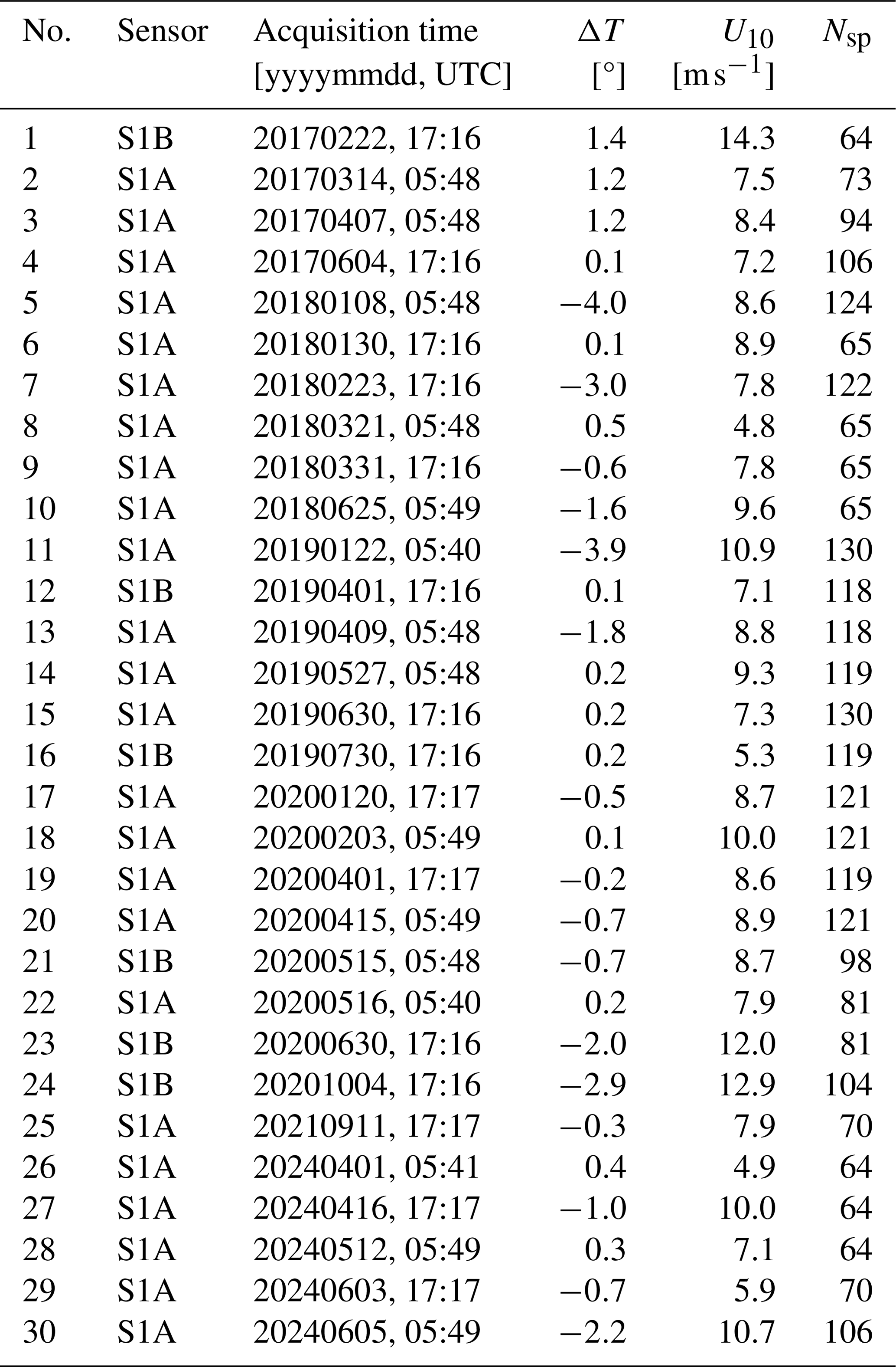
Information about the 30 SAR scenes used in this study is summarised in Table A1. An overview of the corresponding environmental conditions in terms of the average 10 m wind speeds and the air–sea temperature differences in the OWF areas for the SAR acquisition times is shown in Fig. 2a. We emphasise that we did not use the Sentinel-1 Level-2 Ocean (OCN) products, even though they provide wind speed, NRCS, and quality flags. Our assimilation framework requires radiometrically calibrated NRCS values as direct input, not preprocessed wind vectors. Moreover, the OCN products are delivered at coarser resolution and do not allow detailed control of calibration and filtering (e.g. removal of ship signatures, turbine returns and shallow-water artefacts), which is essential for reliable wake inversion.

3.2 Atmospheric model data

Data from the Icosahedral Non-hydrostatic (ICON) atmosphere model run at the German Weather Service (DWD) were used as first-guess information (Reinert et al., 2020). This model has a grid with approximately 7 km resolution and is routinely used for numerical weather prediction (NWP) at DWD. The model data contain hourly wind vectors at 10 m height and information about sea surface temperatures (SSTs) and temperatures at 2 m height (T_2 m).

Figure 2b shows a 2D histogram of wind speeds and air–sea temperature differences $\mathrm{\Delta }T=T_{\mathrm{2}\mathrm{m}}-\text{SST}$ computed inside the German Bight OWF areas for the years 2020–2022. One can see that there is a dominance of unstable situations and that the selected SAR data provide a reasonable representation of typical conditions.

4 Inverse modelling

The general objective of inverse modelling is to achieve good agreement between simulations and observations by adjustment of uncertain model parameters. We have already described the wake model Wake2Sea that is applied to add wakes to existing 2D horizontal wind fields in Sect. 2. To simulate the NRCS measured by a SAR from these wind data, a so-called geophysical model function (GMF) is used. These empirical functions describe the dependency of NRCS on wind speed, wind direction and radar incidence angle and are derived by collocating SAR measurements with in situ wind observations with a typical reference level of 10 m above the sea surface. In this study, the GMF CMOD5.N is used (Portabella et al., 2002; Verhoef et al., 2008; Hersbach, 2008), which was tuned to neutral atmospheric conditions. The choice of GMF is not very critical for the present study because the inversion is based on relative changes in NRCS due to OWF wakes, and absolute NRCS levels, which can vary slightly among different CMOD versions, are of less importance.

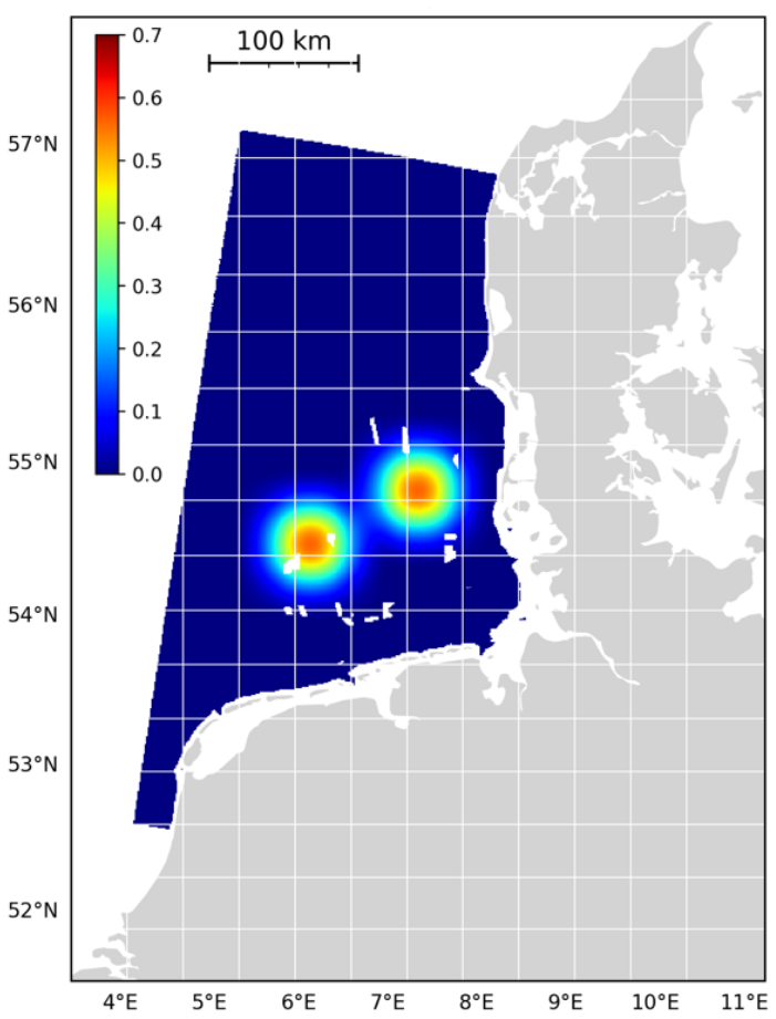
Figure 3 Computational domain used for the Wake2Sea wake simulations and inversions. The 40 km resolution grid for the quadratic B splines used to smooth corrections of the background wind field is superimposed. Two members of the basis are shown in colour-coding as examples. The colour bar refers to the dimensionless spline values.

4.1 Implementation of the inverse modelling scheme

As the wind deficits caused by OWFs have an order of magnitude, which can be comparable to errors in the first-guess model wind field, respective corrections have to be applied in addition to the adjustments to the wake model parameters. Technically, this was done using a 2D spline basis, with two example basis functions shown in Fig. 3. The splines used are quadratic in both dimensions and are defined on a grid with 40 km resolution. One can see that the scale of the splines is larger than the OWF dimensions, and thus it can be expected that the spline corrections are not able to replicate OWF wakes and therefore do not interfere with the wake model.

The quadratic B splines overlap and sum up to unity (Schumaker, 2007). Denoting the spline basis as $B_j,j=\mathrm{1},\mathrm{\dots },N_{\mathrm{sp}}$, the correction of the u and v components of the first-guess wind field for SAR image number k is computed as

$$\begin{array}{}\text{(16)}& {\displaystyle }{u}_{\mathrm{BG}}^k(x,y)=u_{\text{DWD}}^k(x,y)+\sum _{j=\mathrm{1}}^{N_{\mathrm{sp}}}{\mathit{\beta }}_{j,k}^u{B}_j(x,y),\text{(17)}& {\displaystyle }{v}_{\mathrm{BG}}^k(x,y)=v_{\text{DWD}}^k(x,y)+\sum _{j=\mathrm{1}}^{N_{\mathrm{sp}}}{\mathit{\beta }}_{j,k}^v{B}_j(x,y),\end{array}$$

with coefficients ${\mathit{\beta }}_{\mathrm{1},k}^u,\mathrm{\dots },{\mathit{\beta }}_{N_{\mathrm{sp}},k}^u,{\mathit{\beta }}_{\mathrm{1},k}^v,\mathrm{\dots },{\mathit{\beta }}_{N_{\mathrm{sp}},k}^v$. The total control vector α for the optimisation problem is then defined as

$$\begin{array}{}\text{(18)}& \begin{array}{rl}\mathit{\alpha }& =({\mathit{\alpha }}_{\mathrm{wake}},{\mathit{\beta }}_{:,\mathrm{1}}^u,\mathrm{\dots },{\mathit{\beta }}_{:,N_{\mathrm{images}}}^u,{\mathit{\beta }}_{:,\mathrm{1}}^v,\mathrm{\dots },{\mathit{\beta }}_{:,N_{\mathrm{images}}}^v)\\ & \in \mathrm{I}{\mathrm{R}}^{\mathrm{8}+\mathrm{2}{N}_{\mathrm{sp}}{N}_{\mathrm{images}}}.\end{array}\end{array}$$

The control vector dimension is 5728 and thus smaller than 8+2N_spN_images because B splines completely outside of the area covered by the SAR scene were not considered in the inversion. The number of B splines used for each of the SAR images is given in the last column of Table A1. We denote the wind field obtained by feeding the corrected wind field ${\mathit{U}}_{\mathrm{BG}}=(u_{\mathrm{BG}},v_{\mathrm{BG}})$ into the empirical wake model by U_sim(α). The structure of the complete forward model, including the dependencies on the control vector, is depicted in Fig. 4.

Figure 4 Structure of the forward model and the inversion procedure.

The model inversion is then equivalent to the minimisation of the following cost function:

$$\begin{array}{}\text{(19)}& J\left(\mathit{\alpha }\right)={\mathit{\chi }}_{\mathrm{obs}}\left(\mathit{\alpha }\right)+\mathit{\lambda }{\mathit{\chi }}_{\mathrm{prior}}\left(\mathit{\alpha }\right),\end{array}$$

with a scalar weighting factor λ and the two cost function components associated with departures from prior information and differences between observations and simulations:

$$\begin{array}{}\text{(20)}& {\displaystyle }\begin{array}{rl}{\mathit{\chi }}_{\mathrm{prior}}\left(\mathit{\alpha }\right)& =\sum _{k=\mathrm{1}}^{\mathrm{8}}{\displaystyle \frac{({\mathit{\alpha }}_k-{\stackrel{\mathrm{‾}}{\mathit{\alpha }}}_k{)}^{\mathrm{2}}}{({\mathit{\sigma }}_k^{\mathit{\alpha }}{)}^{\mathrm{2}}}}\\ & +\sum _{k=\mathrm{1}}^{N_{\mathrm{images}}}\sum _{j=\mathrm{1}}^{N_{\mathrm{sp}}^j}{\displaystyle \frac{({\mathit{\beta }}_j^{u,k}{)}^{\mathrm{2}}+({\mathit{\beta }}_j^{v,k}{)}^{\mathrm{2}}}{({\mathit{\sigma }}^{\mathit{\beta }}{)}^{\mathrm{2}}}}\end{array}\text{(21)}& {\displaystyle }\begin{array}{rl}{\mathit{\chi }}_{\mathrm{obs}}\left(\mathit{\alpha }\right)& =\sum _{k=\mathrm{1}}^{N_{\mathrm{images}}}\sum _{x\in {\text{SAR}}^k}\\ & \cdot {\displaystyle \frac{\left({\text{NRCS}}_{\mathrm{sim}}\right(U_{\mathrm{sim}}({\mathit{\beta }}^u,{\mathit{\beta }}^v,{\mathit{\alpha }}_{\mathrm{wake}}))-{\text{NRCS}}_{\mathrm{obs}}^k{)}^{\mathrm{2}}}{({\mathit{\sigma }}_{\text{NRCS}}^k{)}^{\mathrm{2}}}},\end{array}\end{array}$$

where the squared differences between the observed and simulated NRCS are summed over all SAR image points x, which fulfil the criteria described in Sect. 3.1. In total, about 40×10⁶ SAR image pixels from N_images=30 images were used in the inversion. For λ=1, the parameters ${\mathit{\sigma }}^{\mathit{\alpha }},{\mathit{\sigma }}^{\mathit{\beta }},{\mathit{\sigma }}_{\mathrm{NRCS}}$ can be interpreted as error standard deviations of the respective control and observation vector components. We will however not use this interpretation rigorously because the structure of the cost function implies some oversimplifying assumptions, particularly concerning the spatial independence of observation errors, and the σ parameters are instead used to control the relative weighting of different components in the cost function. To avoid the dominance of SAR images acquired at high wind speeds and large NRCS values, we chose

$$\begin{array}{}\text{(22)}& ({\mathit{\sigma }}_{\mathrm{NRCS}}^k{)}^{\mathrm{2}}=\text{VAR}({\text{NRCS}}^k)\times {\mathrm{10}}^{\mathrm{5}};\end{array}$$

i.e. the deviations between simulations and observations are scaled with the standard deviation of each image with index k. For the weighting of the prior terms, we chose

$$\begin{array}{}\text{(23)}& {\displaystyle }{\mathit{\sigma }}^{\mathit{\beta }}=\mathrm{1}\mathrm{m}{\mathrm{s}}^{-\mathrm{1}}\text{(24)}& {\displaystyle }{\mathit{\sigma }}_{\mathrm{1}}^{\mathit{\alpha }}={\mathit{\sigma }}_{\mathrm{2}}^{\mathit{\alpha }}=\mathrm{144}\text{(25)}& {\displaystyle }\mathrm{1}/({\mathit{\sigma }}_k^{\mathit{\alpha }}{)}^{\mathrm{2}}=\mathrm{0}\text{for}k=\mathrm{3},\mathrm{\dots },\mathrm{8};\end{array}$$

i.e. the errors in the background wind field are assumed to be of the order of 1 m s⁻¹. The error variance for the Fitch correction parameters is chosen such that a 50 % correction leads to about the same increase in the cost function as a 2 m s⁻¹ background wind field correction over a mesoscale patch, i.e. about 100 km. As a prior, we use ${\stackrel{\mathrm{‾}}{\mathit{\alpha }}}_{\mathrm{1}}=\mathrm{1}$ and ${\stackrel{\mathrm{‾}}{\mathit{\alpha }}}_{\mathrm{2}}=\mathrm{1}$. Technically, α₁ and α₂ were rescaled in the forward model such that the cost function has the standard form commonly used for the L-curve analysis (Hansen and O'Leary, 1993). Very little is known about the remaining control vector components, and they are not regularised at all. We come back to the choice of the weighting factor λ later on in the section.

For each choice of λ, the cost function (Eq. 19) defines a nonlinear least-squares minimisation problem that was solved numerically using a Gauss–Newton method (Press et al., 1992), which would probably be called the incremental 4D-Var method in the context of data assimilation. In this iterative technique, a linearised version of the problem is solved in each iteration step. The equivalent linear system to be solved in each step for the correction Δα of the control vector has the form

$$\begin{array}{}\text{(26)}& \begin{array}{rl}\mathrm{0}& ={\displaystyle \frac{\partial J}{\partial \mathrm{\Delta }\mathit{\alpha }}}=\left[M_{\mathrm{AD}}{H}^T{G}^{-\mathrm{1}}\right(HM\left({\mathit{\alpha }}_i\right)-y){]}^T\\ & +M_{\mathrm{AD}}{H}_{\mathrm{AD}}{G}^{-\mathrm{1}}{H}_{\mathrm{TL}}{M}_{\mathrm{TL}}\mathrm{\Delta }\mathit{\alpha }.\end{array}\end{array}$$

Here, M_AD and M_TL denote the adjoint and tangent linear models of the advection diffusion model described in Sect. 2, respectively. The observation operator H and the respective tangent linear and adjoint operators H_TL and H_AD refer to the CMOD backscattering model. The tangent linear and adjoint models were hand-coded and tested using the dot-product test (Ji, 2009). Both the advection/diffusion and the CMOD imaging models are differentiable, with the exception of the TVD advection scheme, which contains switches. The challenges with respect to the adjoints of advection schemes have been discussed in previous studies (Liu and Sandu, 2008). The challenge of the linear problem (Eq. 26) is that the matrices are not available in explicit form but only as operators in the form of program subroutines; i.e. direct solvers are not practical. The standard approach in such situations is to use a conjugate gradient (CG) method, which is an iterative solver for symmetric systems (Press et al., 1992). With a solution Δα of the system (Eq. 26), the next iteration of the control vector α is given by

$$\begin{array}{}\text{(27)}& {\mathit{\alpha }}_{i+\mathrm{1}}={\mathit{\alpha }}_i+\mathit{\rho }\mathrm{\Delta }\mathit{\alpha },\end{array}$$

where ρ=1 usually leads to a cost function reduction. If that is not the case, smaller step sizes $\mathit{\rho }=\mathrm{0.5},\mathrm{0.25},\mathrm{\dots }$ are tested until a decrease is observed.

All model components and the inversion scheme were implemented in FORTRAN90 and parallelised on a Linux cluster computer. A 2D domain decomposition with 4 by 4 domains is used for the advection/diffusion model and the respective adjoint and tangent linear models. All 30 SAR images are inverted in parallel; i.e. the program requires 480 processors. The model trajectory required in the adjoint model is stored in memory at full temporal resolution, i.e. at 20 s time steps.

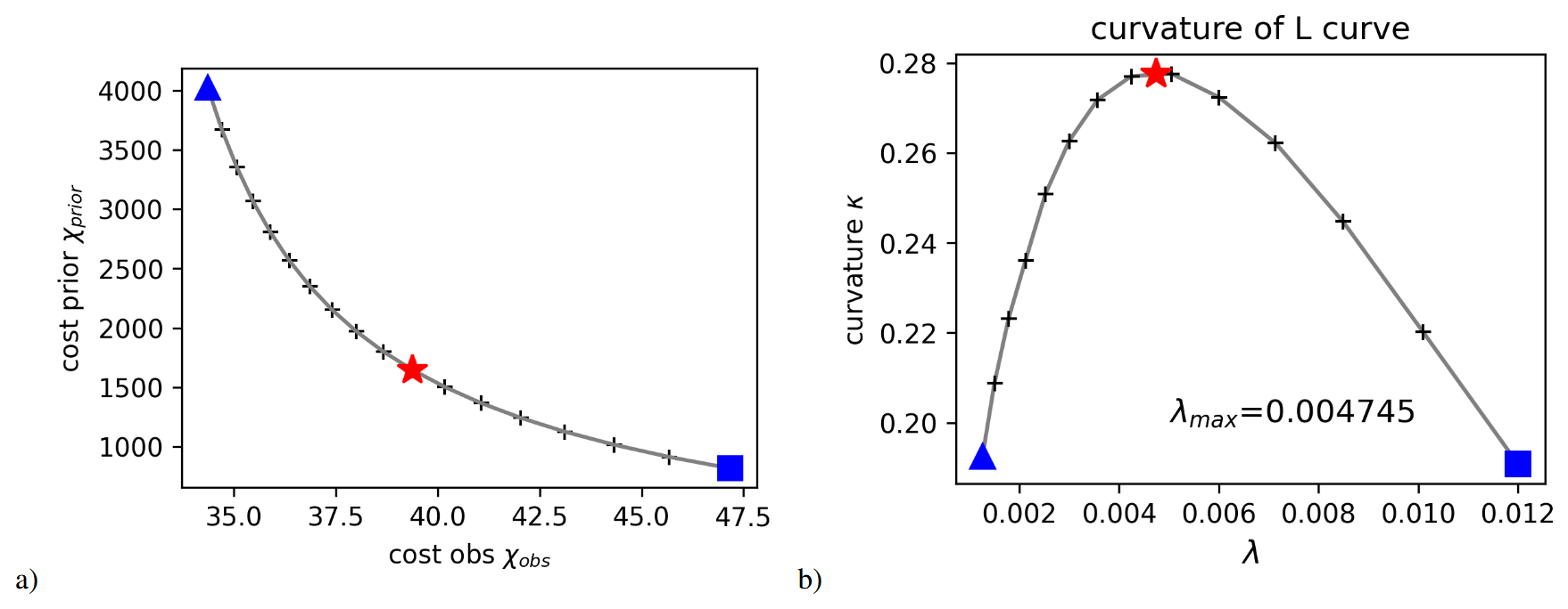
Figure 5 (a) L-curve Γ without taking the logarithm (see Eq. 28). (b) Curvature of Γ as a function of λ with maximum λ_max.

Figure 6 (a) Systematic and non-systematic corrections of the background wind field as a function of λ. (b–d) Components of the estimated control vector α_wake as a function of λ. The red asterisk and blue triangle and square symbols correspond to the maximum curvature point λ_max as well as to the smallest and largest considered λ value.

4.2 L-curve analysis

We now come back to the choice of the parameter λ in Eq. (19), which controls the weighting of the prior and the observation terms. A classical method to determine a reasonable value for λ is the L-curve analysis (Hansen and O'Leary, 1993), where the so-called L-curve defined as

$$\begin{array}{}\text{(28)}& \begin{array}{rl}\mathrm{\Gamma }\left(\mathit{\lambda }\right)& =\left(\log \right({\mathit{\chi }}_{\mathrm{obs}}\left(\mathit{\alpha }\right(\mathit{\lambda }\left)\right)),\log (\left({\mathit{\chi }}_{\mathrm{prior}}\right(\mathit{\alpha }\left(\mathit{\lambda }\right)\left)\right))\\ & =:\left(\widehat{\mathit{\rho }}\right(\mathit{\lambda }),\widehat{\mathit{\eta }}(\mathit{\lambda }\left)\right)\end{array}\end{array}$$

is considered, with α(λ) denoting the solution of the minimisation problem for a given λ, and χ_obs and χ_prior are defined in Eqs. (20) and (21). The L-shaped curve obtained for the inversion problem described in the previous section is shown in Fig. 5a, omitting the logarithm in Eq. (28). The triangle and square symbols correspond to the smallest and largest considered λ values, respectively. The general idea is that it does not make sense to look at solutions which are very far on the left or very far on the right because they are either replicating noisy observations or simply reproducing prior knowledge. It can be justified that a choice of λ that maximises the curvature

$$\begin{array}{}\text{(29)}& \mathit{\kappa }\left(\mathit{\lambda }\right)={\displaystyle \frac{{\widehat{\mathit{\rho }}}^{\prime }{\widehat{\mathit{\eta }}}^{\prime \prime }-{\widehat{\mathit{\rho }}}^{\prime \prime }{\widehat{\mathit{\eta }}}^{\prime }}{\left(\right({\widehat{\mathit{\rho }}}^{\prime }{)}^{\mathrm{2}}+({\widehat{\mathit{\eta }}}^{\prime }{)}^{\mathrm{2}}{)}^{\mathrm{3}/\mathrm{2}}}}\end{array}$$

of Γ is a reasonable compromise between these two extremes (Hansen and O'Leary, 1993). The computed curvature for our case is shown in Fig. 5b, indicating a pronounced maximum at around λ_max=0.004791. The wake model parameters estimated for different choices of λ are summarised in Fig. 6b–d. The relatively smooth dependence of the solution vector on λ indicates a stable performance of the inversion procedure. The red asterisks indicate the solutions corresponding to the maximum curvature of Γ. A plot for α₁,α₂ is not shown because the departures from the first guess were negligible. Our general interpretation of the curves in Fig. 6b–d is that the inversion scheme uses the wake model to compensate for errors in the background wind field if the prior is weighted more strongly. As these background errors typically have a larger spatial scale than the OWF wakes, the inversion tends to diffuse the simulated wakes, e.g. by increasing the horizontal diffusion coefficient ν_H or by making the wakes longer by decreasing α₃. Figure 6a shows the standard deviation for the magnitude of the wind speed corrections as well as the mean systematic correction of the u and v components as a function of λ. One can see that the magnitude of the systematic corrections is below 5 cm s⁻¹ and that the non-systematic corrections start to grow quite rapidly below λ_max.

Table 2 Estimates for the control vector α_wake used in the Wake2Sea model, which were obtained with the 4D-Var inversion procedure.

5 Inversion results

The exact values for the wake model control vector components at the maximum curvature point are summarised in Table 2. The positive value for α₅ indicates that, as expected, the vertical diffusion is higher in unstable situations. The negative value for α₄ suggests that the sink term for the deficit is smaller for high deficits, which are found closer to the OWFs. This seems to be slightly counter-intuitive because higher deficits are associated with stronger vertical shear and turbulence production. We can only speculate that this might have to do with the time the turbulence requires to penetrate the layers above the rotor discs, eventually increasing the downward momentum flux.

The value of roughly ν_H=990 m² s⁻¹ for the horizontal diffusion emphasises the importance of using higher-order advection schemes in the simulation. The use of a first-order upwind scheme in this study would have resulted in a numerical diffusion of the order of 0.5 U₁₀Δx≈5000 m² s⁻¹, i.e. significantly larger than the estimated physical diffusion.

The values for α₇ and α₈ indicate that the ratio of the deficit at 10 m height is about 36 % of the deficit averaged over the first 200 m on average (see Eqs. 14 and 11).

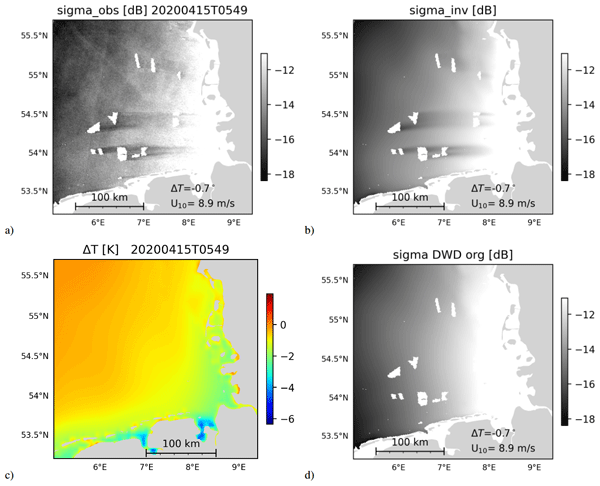
Figure 7 Example of an inversion for the Sentinel-1A SAR scene acquired on 15 April 2020 at 05:49 UTC (Copernicus Sentinel data, 2020) with measured NRCS (a), best simulated NRCS (b), sea surface temperature difference (c) and NRCS simulation based on the original DWD atmospheric model data without OWF parameterisation (d).

As an example, Fig. 7 shows 1 of the 30 inversions for a SAR scene acquired on 15 April 2020 at 05:49 UTC. This was a slightly unstable situation with wind speeds of around 9 m s⁻¹ from westerly directions. The air–sea temperature map used in the inversion is shown in Fig. 7c, exhibiting a typical increase towards the land caused by stronger warming of water in the shallow near-coastal areas. Comparing the observed NRCS in Fig. 7a with the best simulation in Fig. 7b shows good agreement of the multiple wake structures in terms of intensity and size. The NRCS simulation without the wake model and background corrections of the wind field can be found in Fig. 7d. It can be seen that the original DWD wind field is already quite consistent with the SAR measurements. Smaller corrections are mainly applied in the near-coastal areas with stronger NRCS gradients.

Figure 8 (a) Number of images in the Sentinel-1 dataset of 30 images that cover different locations in the German Bight. (b) Relative improvement of agreement between observed and simulated radar cross section achieved by the fitting, if the original DWD wind data are used as reference. (c) The same as (b) but here the improvement due to the empirical wake model is shown using the large-scale corrected DWD wind data as a reference. (d) Standard deviation of wind corrections applied on a scale of 40 km and above.

A statistical overview of the inversions is presented in Fig. 8. A map indicating the number of SAR acquisitions used at each location in the German Bight is shown in Fig. 8a. One can see that for most of the central part, close to 30 images are available. Only in the northern, western and near-coastal margins does the coverage drop to 25 images or below. Figure 8b shows the relative improvement of the RMSE comparing the NRCS simulations based on DWD data without wakes and background corrections with the best inversion results. One can see a relatively homogeneous improvement between 80 % and 100 %. The standard deviation of the respective background wind speed corrections is given in Fig. 8d. For the most part, the standard deviations are between 0.6 and 0.8 m s⁻¹, which is consistent with the model error levels reported in previous studies (Rieger et al., 2021). Higher correction values are found in some areas with lower data availability, in particular at the western margin, and these are likely dominated by some individual cases, which required stronger corrections. The overall biases for the zonal and meridional wind components are −0.04 and −0.01 m s⁻¹, respectively; i.e. the systematic inconsistencies between DWD data and SAR measurements are small.

In Fig. 8c, RMSE improvements are shown again, but this time the reference is the simulations including the background wind corrections; i.e. the plot isolates the improvements achieved by the empirical wake model alone. For that reason, the main relative improvements between 40 % and 80 % are found in the neighbourhood of the offshore wind farms, with a particular focus on the eastern side corresponding to the dominant westerly wind directions.

Figure 9 Mean relative (a) and absolute (b) wind speed deficits computed with the empirical model Wake2Sea for 2020. (c, d) Respective standard deviation (c) and 90 % percentile of deficit.

5.1 Simulations with Wake2Sea for a complete year

As a first application of the empirical model Wake2Sea, OWF wakes were added to a complete year of DWD atmospheric model data. Figure 9 shows respective maps of estimated deficits at 10 m height for the year 2020. The wake model was applied in the same way as in the inversion; i.e. hourly model data were used as input, and a time step of 20 s was used in the explicit scheme. The only adjustment that was necessary is related to very high wind speeds above 30 m s⁻¹ that occurred during some short periods in that year. Although we used a cut-out wind speed of 25 m s⁻¹, above which the deficit production is switched off, spurious deficits generated at previous time steps can still exist and lead to instabilities. For this reason, model wind vectors were scaled down to 30 m s⁻¹ in those situations.

Figure 9a shows the mean percentage deficits averaged over the entire year. It can be seen that the maximum average deficits with values around 8 % are concentrated in a small area around the OWFs. Averages of the absolute wind speed reductions are shown in Fig. 9b. One can see that the wind farm cluster in the southwesterly part causes a reduction of at least 0.2 m s⁻¹ within an area of almost 100 km × 100 km. The deficit standard deviation displayed in Fig. 9c illustrates that the area where wakes can occur from time to time is significantly larger than suggested by the mean deficit in Fig. 9a. To get an impression of stronger shadowing effects, Fig. 9d shows the 90 % deficit percentile, i.e. deficit values that are exceeded in 10 % of the cases. One can see that there are larger areas, in particular between and inside the OWFs, with deficit values of 15 % and above.

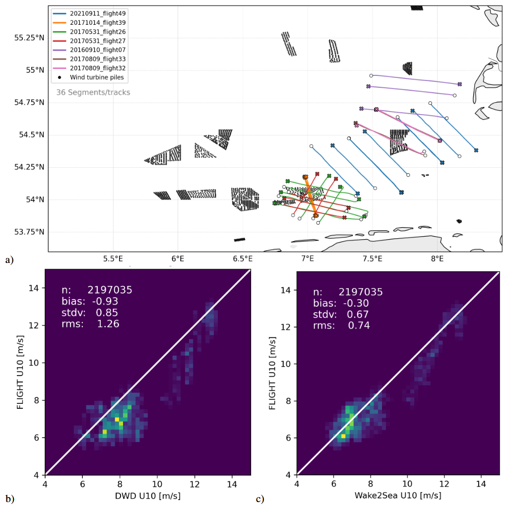
Figure 10 Airborne flight segments used for independent validation (36 segments) shown over the German Bight with wind turbine locations superimposed (a). The segment sample regions within and downstream of major offshore wind farm clusters. Comparison of airborne observed wind speed with (b) DWD 10 m wind speeds and (c) Wake2Sea-corrected winds for all collocated flight data. Statistics (bias, standard deviation, RMSE) are shown in each panel (n=2 197 035 collocated points). Wake2Sea reduces both systematic and random errors relative to the baseline.

5.2 Independent validation of Wake2Sea with airborne campaign data

To provide an independent evaluation of Wake2Sea beyond the SAR-based inversion, we compare modelled 10 m wind speeds with airborne campaign measurements collected over and downstream of offshore wind farms. The airborne data are not used in the inversion and are used only for evaluation. Collocated comparisons are performed along 36 flight segments (Fig. 10a). Because strict temporal coincidence between aircraft and satellite observations is rarely achievable, we allow a temporal tolerance of 2 h relative to Sentinel-1 overpasses when selecting transects for the validation. This represents a compromise between data availability and maintaining comparable mesoscale conditions during the validation period.

Wake2Sea is evaluated against airborne wind measurements collected during the WIPAFF and XWAKES field campaigns (Bärfuss et al., 2019; Rausch et al., 2023). Airborne wake observations from WIPAFF have been widely used as an independent benchmark to evaluate wake representations in mesoscale simulations with wind farm parameterisations (including WRF) and wake-recovery behaviour in the German Bight (Siedersleben et al., 2018, 2020; Platis et al., 2018, 2021). The selected transects span multiple dates and wind farm clusters, providing a geographically and temporally diverse validation dataset. To enable a physically consistent comparison with modelled near-surface winds, the aircraft observations were adjusted to a common reference height of 10 m using a bulk-stability-corrected logarithmic profile based on Monin–Obukhov similarity theory (bulk MOST), with stability information derived from the flight measurements.

Figure 10a gives an overview of the flight tracks used in the comparisons. Figure 10b and c summarises the statistical agreement between airborne observations and the original DWD 10 m winds (Fig. 10b) as well as the same winds after applying Wake2Sea (Fig. 10c). The comparison demonstrates a clear improvement when using Wake2Sea relative to the DWD background wind field alone. In the 2D histograms, the Wake2Sea estimates are more tightly clustered around the diagonal than the corresponding DWD values, indicating both reduced systematic deviation and lower scatter with respect to the aircraft observations. The error metrics corroborate this improvement. The mean bias decreases in magnitude from −0.93 m s⁻¹ (DWD) to −0.30 m s⁻¹ (Wake2Sea), the standard deviation decreases from 0.85 to 0.67 m s⁻¹ and the root-mean-square error declines from 1.26 to 0.74 m s⁻¹. These results indicate that the empirical wake parameterisation adds substantial predictive skill and captures the wake-affected offshore flow more realistically than the background meteorological forcing alone.

5.3 Comparisons with FINO-1 in situ measurements

As an independent validation of the inversion results, comparisons were performed with measurements taken at the research platform FINO-1. We emphasise that FINO-1 wind measurements are not assimilated and were not used to tune any Wake2Sea parameters; they are used only for an independent in situ evaluation of the results. The location of the platform is indicated by the black triangle in Fig. 1a. There are two main challenges in this comparison. (1) The lowest FINO-1 measurement is at 34 m height, i.e. significantly above the 10 m reference level used in this study. (2) The FINO-1 platform is located in the centre of a large wind park cluster; i.e. the wakes measured by the platform are more inner-park wakes rather than external wakes in nature. In this context, it is important to remember that the interior of wind parks was excluded in the inversion because of radar reflections from the turbine structures; i.e. the empirical model is not optimised for inner-wind-park wakes.

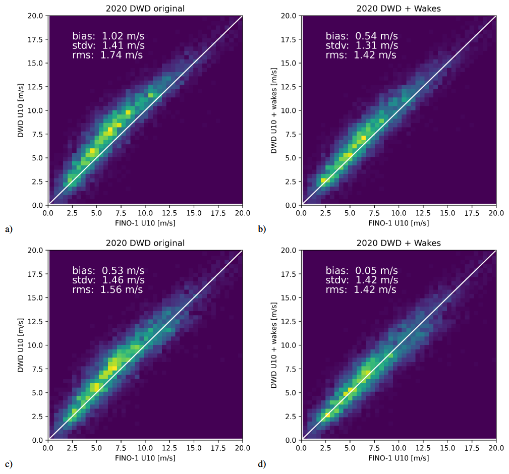
Figure 11 Comparison of FINO-1 measurements with DWD model 10 m wind speeds without wakes (a, c) and with Wake2Sea-simulated wakes (b, d). Neutral conditions were assumed in the extrapolation from 34 to 10 m in (a) and (b). Turbulence due to wakes was considered in the extrapolation in (c) and (d).

The 34 m FINO-1 measurements were extrapolated down to 10 m assuming a neutral wind profile $U\left(z\right)=u^{*}\log (z/z_{\mathrm{0}})/\mathit{\kappa }$ in combination with the Charnock equation:

$$\begin{array}{}\text{(30)}& z_{\mathrm{0}}=\mathrm{0.015}(u^{*}{)}^{\mathrm{2}}/g\end{array}$$

with gravitational acceleration g, roughness length z₀, friction velocity u^* and a Karman constant κ.

The empirical model Wake2Sea was used to add OWF wakes to a complete year of DWD model data, resulting in a dataset for wind speeds U₁₀ with hourly sampling. The comparison of the original DWD data for the year 2020 with the extrapolated FINO-1 measurements is shown in Fig. 11a. One can see a significant bias of about 1 m s⁻¹, which is consistent with the missing OWF wakes in the model data. The corresponding comparison with the model data including wakes can be found in Fig. 11b. In this case the bias is reduced by a factor of 2, and the standard deviations and the RMSE are reduced significantly as well. Considering the remaining bias of 0.54 m s⁻¹, one can now argue that the assumption of a neutral boundary layer is not realistic, particularly inside a wind park cluster. Inside the wakes, turbulence and vertical mixing are increased, and one can expect that the wind speeds at 10 and 34 m are in closer agreement than suggested by the theoretical log profile. Following this argument, a second comparison was performed in which the 10 m wind was assumed to be equal to the 34 m FINO-1 measurement for those cases where the wake model indicated a wind deficit of at least 3 %. These estimates were then compared to model data with and without wakes as before. The results shown in Fig. 11c and d indicate that the bias is now reduced by a factor of 10, with a remaining value of 0.05 m s⁻¹, and the standard deviation is also slightly improved.

In any case, the wake model improves the agreement of the model data with the FINO-1 observations, despite the fact that the model was never tuned to these interior wind cluster conditions. We are not claiming that our procedure for introducing additional vertical mixing is highly accurate, but the analysis shows that the reasonable assumption of additional mixing leads to further reductions in bias. The order of magnitude of the respective deviations is now close to error levels associated with assumptions about the vertical profiles, and this calls for more dedicated in situ measurements in offshore wind farm areas.

6 Theoretical considerations of Wake2Sea

In this section, we illustrate some properties of the Wake2Sea model with the parameters estimated from the satellite dataset. We would like to emphasise again that we are not claiming that the model is dynamically consistent in all aspects, but rather that we are putting the observational information at the centre of this study. In this context, we point out that state-of-the-art mesoscale and LES models are far from perfect as well (Ouro et al., 2025).

6.1 Analytical downstream deficit profiles

A rough idea about the shape of the wakes produced with the Wake2Sea model can be obtained by assuming that the background wind field u is constant, neglecting lateral diffusion and considering the stationary case with $\frac{\partial D}{\partial t}=\mathrm{0}$. If we further assume α₄=0, the solution for D is given by

$$\begin{array}{}\text{(31)}& D\left(x\right)\approx D_{\mathrm{0}}\exp (-{\mathit{\alpha }}_{\mathrm{3}}^{\mathrm{2}}x/u),\end{array}$$

where D₀ is the initial deficit, and x is the distance from the wind farm. If the deficit dependence in the sink term (see Eq. 10) is expanded to quadratic order, i.e.

$$\begin{array}{}\text{(32)}& {\displaystyle \frac{\partial D}{\partial t}}\approx \mathrm{\dots }-D{\mathit{\alpha }}_{\mathrm{3}}^{\mathrm{2}}(\mathrm{1}+\mathrm{2}{\mathit{\alpha }}_{\mathrm{4}}D)(\mathrm{1}-{\mathit{\alpha }}_{\mathrm{5}}\mathrm{\Delta }T{)}^{\mathrm{2}}+\mathrm{\dots },\end{array}$$

the stationary solution is given as

$$\begin{array}{}\text{(33)}& D\left(x\right)\approx {\displaystyle \frac{{\mathit{\xi }}_{\mathrm{1}}}{\exp ({\stackrel{\mathrm{‾}}{\mathit{\alpha }}}_{\mathrm{3}}x/u)-\mathrm{2}{\mathit{\alpha }}_{\mathrm{4}}{\mathit{\xi }}_{\mathrm{1}}}}\end{array}$$

with

$$\begin{array}{}\text{(34)}& {\stackrel{\mathrm{‾}}{\mathit{\alpha }}}_{\mathrm{3}}={\mathit{\alpha }}_{\mathrm{3}}(\mathrm{1}-{\mathit{\alpha }}_{\mathrm{5}}\mathrm{\Delta }T)\end{array}$$

and

$$\begin{array}{}\text{(35)}& {\mathit{\xi }}_{\mathrm{1}}={\displaystyle \frac{D_{\mathrm{0}}}{\mathrm{1}+\mathrm{2}{\mathit{\alpha }}_{\mathrm{4}}{D}_{\mathrm{0}}}}.\end{array}$$

Figure 12a shows a comparison of the linear and quadratic approximation of the stationary deficit profiles and the solution obtained by numeric integration of the complete sink expression for neutral conditions; i.e. ΔT=0. One can see that the quadratic approximation is in very good agreement with the full nonlinear solution and that the non-linearity leads to a slightly slower decay of the wake near the wind farm compared to the linear solution.

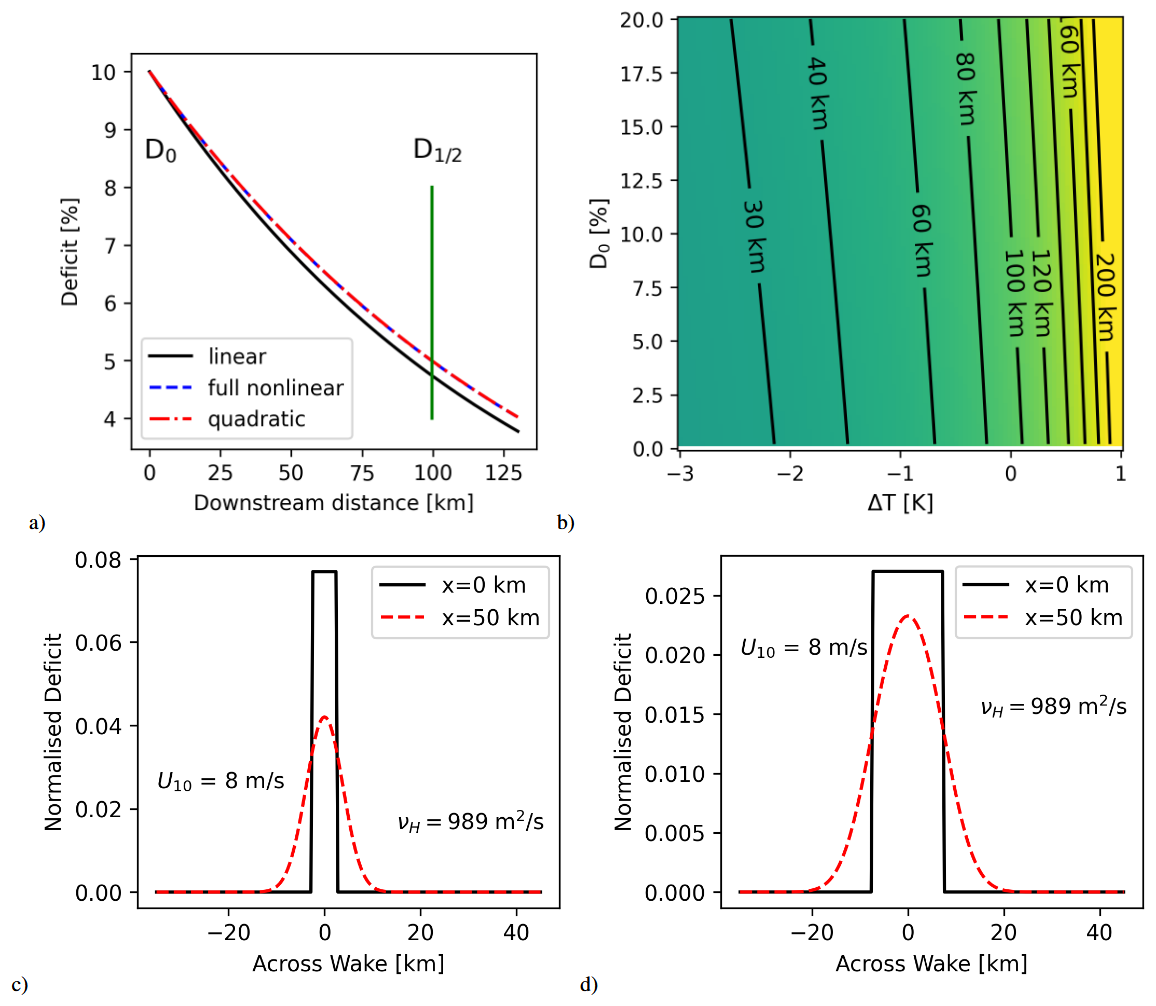
Figure 12 (a) Theoretical deficit profiles computed using the linear approximation (Eq. 31) (black curve), the quadratic approximation (Eq. 33) (red dashed dotted) and the numerical integration (dashed blue) assuming neutral conditions. (b) Half-decay distance $D_{\mathrm{1}/\mathrm{2}}$ in the quadratic model as a function of the initial deficit D₀ and the air–sea temperature difference for a wind speed of 8 m s⁻¹. (c, d) Theoretical across-wake profiles for u=8 m s⁻¹ at downstream distances of x=0 km and x=50 km using the lateral diffusion coefficient ν_H estimated based on SAR data. The initial wake width is 10 km (c) and 30 km (d).

The distance at which the deficit has dropped to half of the initial value is then given by

$$\begin{array}{}\text{(36)}& D_{\mathrm{1}/\mathrm{2}}={\displaystyle \frac{u}{{\stackrel{\mathrm{‾}}{\mathit{\alpha }}}_{\mathrm{3}}^{\mathrm{2}}}}\log \left(\mathrm{2}{\mathit{\xi }}_{\mathrm{1}}\right(D_{\mathrm{0}}^{-\mathrm{1}}+{\mathit{\alpha }}_{\mathrm{4}}\left)\right).\end{array}$$

Figure 12b shows this parameter as a function of air–sea temperature difference and initial deficit D₀ for a wind speed of 8 m s⁻¹. According to Eq. (36), a simple linear scaling can be applied to obtain $D_{\mathrm{1}/\mathrm{2}}$ for other wind speeds. One can see that there is a pronounced stability dependency and a relatively weak impact of the initial deficit D₀.

6.2 Horizontal diffusion of wake

The estimated lateral diffusion ν_H leads to an across-wake expansion that can be analysed analytically based on some simplifying assumptions. The wake expansion has been addressed in previous studies, e.g. Frandsen et al. (2006); however this is the first time this effect is estimated for the near-surface deficits using satellite observations. If we assume that the across-wake profile has a top-hat shape as suggested by Lanzilao and Meyers (2025) at a distance x=0 km from the wind farm and furthermore that the deficit is advected by a constant velocity u, then the evolution of the across-track deficit profile as a function of x can be described as

$$\begin{array}{}\text{(37)}& D\left(y\right)={\displaystyle \frac{D\left(x\right)}{\mathrm{2}}}(\text{erf}\left({\displaystyle \frac{y+a}{\sqrt{\mathrm{4}{\mathit{\nu }}_{H}x/u}}}\right)-\text{erf}\left({\displaystyle \frac{y-a}{\sqrt{\mathrm{4}{\mathit{\nu }}_{H}x/u}}}\right)),\end{array}$$

where erf denotes the error function, y is the across-track coordinate with y=0 corresponding to the centre and D(x) is the along-wake deficit profile. To separate the deficit decay due to the lateral diffusion from the effects caused by vertical diffusion, we simply assume D(x)=const. Figure 12c and d shows examples of across-wake profiles at x=0 km (solid black line) and at x=50 km (red dashed line) for u=8 m s⁻¹. The initial wake width is 10 km in Fig. 12c and 30 km in Fig. 12d. One can see that the lateral diffusion has a smaller effect on the maximum deficit if the wake is wider because it takes more time for the diffusive lateral fluxes to change the shape of the profile.

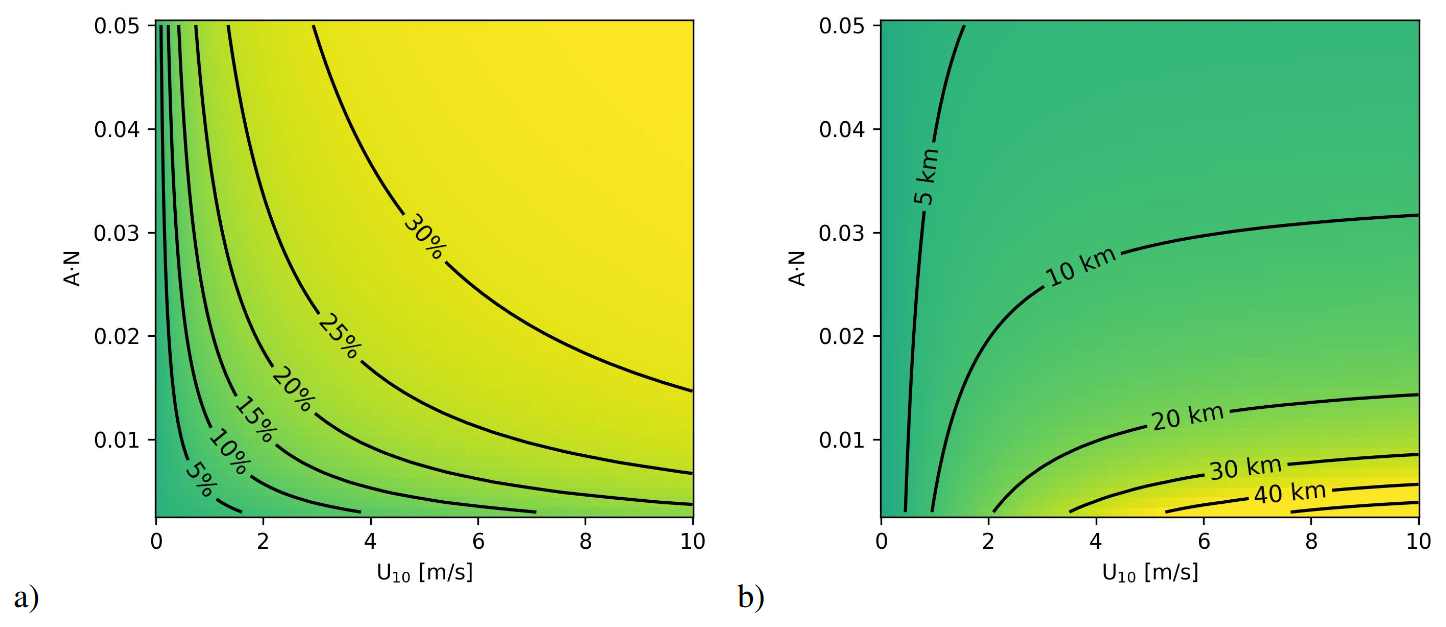
Figure 13 (a) Maximum deficit $D_{\mathrm{10}\mathrm{m}}^{\mathrm{\infty }}$ at 10 m as a function of wind speed and relative normalised rotor area NA in big wind parks. (b) The same as (a) for the half distance $x^{\mathrm{1}/\mathrm{2}}$ required to reach $D_{\mathrm{10}\mathrm{m}}^{\mathrm{\infty }}$.

6.3 Wake growth in large wind parks

Another interesting question is the maximum deficit that can be reached in very large wind parks. As the wind speed reduction caused by the wake is included in the source term in Eq. (7), the deficit cannot grow above 100 %, and there is a well-defined saturation limit. If the linear approximation is used for the vertical diffusion, i.e. α₄=0, and furthermore a constant C_T value is assumed, the following solution is obtained inside the wind park:

$$\begin{array}{}\text{(38)}& D\left(x\right)=D^{\mathrm{\infty }}(\mathrm{1}-\exp (-x({\mathit{\alpha }}_{\mathrm{3}}^{\mathrm{2}}/u+c_{\mathrm{1}})\left)\right),\end{array}$$

where x=0 defines the upstream boundary of the park, and

$$\begin{array}{}\text{(39)}& {\displaystyle }{c}_{\mathrm{1}}=\mathrm{0.5}N{C}_{\mathrm{T}}A/\mathrm{d}Z\text{(40)}& {\displaystyle }{D}^{\mathrm{\infty }}={\displaystyle \frac{c_{\mathrm{1}}u}{{\mathit{\alpha }}_{\mathrm{3}}^{\mathrm{2}}+c_{\mathrm{1}}u}}.\end{array}$$

The distance after which half of the saturation deficit D^∞ is reached is then given by

$$\begin{array}{}\text{(41)}& x^{\mathrm{1}/\mathrm{2}}={\displaystyle \frac{\log \left(\mathrm{2}\right)}{{\mathit{\alpha }}_{\mathrm{3}}^{\mathrm{2}}/u+c_{\mathrm{1}}}}.\end{array}$$

Figure 13a and b shows $x^{\mathrm{1}/\mathrm{2}}$ and $D_{\mathrm{10}\mathrm{m}}^{\mathrm{\infty }}\approx {\mathit{\alpha }}_{\mathrm{7}}^{\mathrm{2}}{D}^{\mathrm{\infty }}$ as a function of wind speed U₁₀ and the normalised rotor area N⋅A for C_T=0.8. One can see that the internal wakes require longer distances to build up under high-wind-speed conditions and in OWFs with lower turbine density. The model predicts that for slightly higher wind speeds, the deficit can grow well beyond 30 % in very dense wind parks. We have to emphasise again that the model was not tuned to internal wake measurements, and it is implicitly assumed that the vertical deficit diffusion can be described with the same parameterisation inside and outside OWFs. Furthermore, this analysis does not include the horizontal diffusion discussed in the previous section (Sect. 6.2); i.e. conceptually it refers to an infinitely wide wake. The comparison of the Wake2Sea model results with FINO-1 data in Sect. 5.3 suggest at least that there is no obvious overestimation of deficits inside of wind park clusters.

7 Conclusions and outlook

A 2D semi-empirical model for wind speed deficits near the sea surface downstream of offshore wind parks was fitted to satellite SAR data. The Wake2Sea model enables the inclusion of OWF wakes a posteriori into existing atmospheric model datasets at significantly lower computational costs compared to complete re-runs of full-blown 3D atmospheric models. The optimisation of the method for near-surface wind deficits makes Wake2Sea an attractive tool for oceanographers, who need to include OWFs in the atmospheric forcing for ocean model simulations. The application of the method to wind fields obtained from the operational German weather forecast system leads to a significantly improved agreement with the satellite observations. Comparisons with independent measurements taken at the FINO-1 measurements confirmed that the empirical model is able to reduce biases in meteorological model datasets not including OWF wake effects. Consideration of turbulence associated with OWF wakes in the extrapolation from 34 to 10 m height leads to further improvements in the agreement between wake model results and in situ observations. Similarly, the inclusion of wakes in the DWD data significantly improved the agreement with independent airborne campaign data acquired during the WIPAFF and XWAKES projects.

The parameterisation of the empirical model allowed adjustments to the standard Fitch OWF parameterisation in terms of the momentum sink scaling and the dependence of the thrust curve on wind speed; however it turned out that the results of the inversion procedure only deviate marginally from the standard formulations found in literature.

The sink term for the wind deficit, which is related to vertical momentum diffusion, was found to exhibit a clear dependency on the air–sea temperature difference with lower deficit diffusion in stable conditions of the ABL. The sink term also showed a slight dependency on the deficit itself, with lower diffusion at higher deficits. Further studies have to clarify whether this reflects an actual physical process or if this is an effect associated with the simplified representation of the 3D dynamics in the 2D empirical model.

The inversion results indicated that the wind speed deficit at 10 m height is about 36 % of the deficit averaged over the first 200 m of the ABL. The inversions did not show a significant dependency of this ratio on the deficit itself. It is important to emphasise that the inversion scheme can potentially compensate for possible deficiencies in the Fitch parameterisation by adjustment of the velocity ratio. A thorough optimisation of the OWF parameterisation would require additional information about vertical wind speed profiles inside and outside of wake regions.

We would like to emphasise that the tuning of the wake model to satellite data in the German Bight leads to limitations with regard to general applicability. For example, the wind directions in the German Bight are predominantly from the north and west, which means that many situations are characterised by fully developed marine boundary layers and less by intermediate boundary layers associated with the close proximity of land. We think that a more thorough treatment of intermediate boundary layer cases would require explicit prognostic inclusion of turbulent kinetic energy (TKE) in the model. Because of the substantially higher complexity and the corresponding challenges in the inversion, we decided to address this issue in a separate study.

To our knowledge, this study represents the first attempt to achieve and demonstrate quantitative consistency between a physical-based OWF wake model with SAR observations considering a larger variety of wind speed and stability conditions. Despite its simplicity, the model is able to capture major characteristics of the observed wakes. The approach has natural limitations because of the 2D treatment of wakes and the missing simulation of turbulence. It will be the subject of follow-up studies to address some of these deficits while maintaining an acceptable increase in computational costs. In this context, we think that dedicated in situ measurements in the ABL between the sea surface and hub height would be of great value for the further optimisation of OWF wake models for oceanographic applications.

Appendix A: List of Sentinel-1 SAR data used

Table A1 Sentinel-1A and Sentinel-1B SAR scenes acquired over the German Bight, which were used in the presented analysis. ΔT denotes the air–sea temperature difference (T_2 m−SST) and U₁₀ refers to the 10 m wind speed. The last column gives the number of B spline basis functions used in the correction of the background wind field (compare Eqs. 16, 17).