
the Creative Commons Attribution 4.0 License.
the Creative Commons Attribution 4.0 License.
 | 08 Jul 2026
Large-eddy simulation of the IEA 15 MW wind turbine using a two-way coupled fluid–structure interaction model
Claudio Bernardi
Stefania Cherubini
Felice Manganelli
Giacomo Della Posta
Stefano Leonardi
Pietro De Palma
The aim of this work is to study the aeroelastic response of the IEA 15 MW Reference Wind Turbine (RWT)using a high-fidelity fluid–structure interaction solver that combines large-eddy simulation with a modal computational structural dynamics solver through a two-way coupling. The fluid solver employs the actuator line model to simulate the interaction between the turbine blades and the fluid and the immersed-boundary method to model the presence of the tower and nacelle. The results are compared with those obtained by the OpenFAST software, which is a well-known numerical tool for engineering predictions. A series of simulations have been performed with and without the presence of the tower and nacelle to better understand the effects of these components on flow structures and structural deformations. The largest discrepancies among the solvers have been observed in correspondence with the blade passage in front of the tower, which induces an abrupt alteration in the local incidence angle of the flow. Moreover, by comparing the outcomes of different structural approximations, it has been established that taking into account the torsional degree of freedom affects the deformations, aerodynamic loads, and power coefficient considerably. On the other hand, the non-linearity of the solver appears to have a weak effect on the same quantities.
- Article
(8433 KB) - Full-text XML
- BibTeX
- EndNote


Wind energy has become a crucial component of the global transition towards renewable energy sources. The increasing demand for clean energy has led to the development of large-scale wind turbines, such as the IEA 15 MW offshore wind turbine developed within IEA Wind Task 37 (Gaertner et al., 2020a). This turbine, with a rotor diameter of 240 m and blades measuring 117 m in length, represents a new frontier in wind energy technology (Gaertner et al., 2020b), and research is currently pointing towards even larger rotors, reaching 22 MW of power production (Zahle et al., 2024). The increasing scale and flexibility of such newly designed turbines present significant engineering challenges, particularly in predicting their aeroelastic response (Burton et al., 2011; Zheng et al., 2023). As turbines grow in size, their structural components, especially the blades, are subject to complex aerodynamic forces that cause deformations, which, in turn, affect the aerodynamic loads. Understanding these interactions is essential to improve the performance, reliability, and longevity of large-scale wind turbines (Manwell et al., 2010). In the worst cases, aeroelastic instabilities such as edgewise instability and flutter might even lead to blade damage, as reported for the Lunderskov Mobelfabrik 19 m wind turbine blades (Moeller, 1997), with devastating effects on the turbine performance.
Aeroelasticity is critical in the design and analysis of modern wind turbines. Aeroelastic phenomena such as dynamic stall, flutter, and their effects on fatigue loadings can have significant effects on turbine performance, particularly as the blade length increases (Hansen, 2007). These blades experience varying aerodynamic forces along their span, which can lead to substantial deformations. When blades deform, they alter the local flow field, which, in turn, modifies the aerodynamic loads acting on them. This feedback loop between aerodynamic forces and structural deformation makes it very difficult to predict modern large-scale turbine performance under real-world operating conditions (Vermeer et al., 2003; Wang et al., 2016a). Accurate evaluation of these interactions is key for ensuring turbine efficiency and structural integrity, especially in offshore environments where wind conditions are more severe (Bayati et al., 2017).
The numerical modeling of the blades in most of the numerical aeroelastic codes used nowadays (Schepers et al., 2021) is accomplished by the blade element momentum (BEM) model due to its robustness and low computational cost. It has been shown in the framework of the IEA WIND Task 47 (Boorsma et al., 2023, 2024) that, if properly tuned, BEM can be a valuable engineering-type solver, complementary to higher-fidelity ones which also have higher computational costs. However, BEM still has some limitations since it relies on simplifying assumptions regarding the impinging flow, such as models of dynamic stall, dynamic inflow, yaw and tilt flows, and corrections of the aerofoil data for taking into account three-dimensional effects and tip losses. More computationally expensive models exist, such as panel methods and, in general, potential flow solvers and/or free-vortex wake methods, as well as the actuator disk methods. Panel and free-wake vortex methods are able to capture unsteady blade and/or rotor aerodynamics with good accuracy under different operating conditions (including off-design) whenever massive flow separation phenomena do not occur (Boorsma et al., 2018; Ribeiro et al., 2023). However, those models need reference high-fidelity data in order to refine and/or assess the reliability of these lower-fidelity models. Therefore, the application of computational fluid dynamics (CFD) to full-scale turbines is needed as a reference for describing the complex aerodynamics of the flow field accurately (Sørensen, 2011) although limited to a low number of flow cases due to its high computational cost.
However, coupling three-dimensional CFD simulations with computational structural dynamics (CSD) solvers, taking into account the deformation of the blade, is not trivial. Three-dimensional structural finite-element models are, in fact, able to fully describe the complex shape of a wind turbine blade, but, although accurate, these models are computationally expensive and hard to implement, leading to only a few examples of coupling with CFD codes (Bazilevs et al., 2011; Yu and Kwon, 2014). Since wind turbine blades are slender structures, their structural modeling can be more easily achieved using beam models, where the blade is discretized as a series of one-dimensional beam elements, each characterized by a given cross-sectional stiffness and mass per unit length. One-dimensional beam models can either be modal – since natural frequencies and mode shapes of a turbine are directly related to the natural frequencies of its blades – or rely on the geometrically exact beam theory, including non-linear effects (Sabale and Gopal, 2019).
Due to their ability to provide a rapid evaluation of the turbine performance, numerical tools based on the BEM approach equipped with aeroelastic modules based on one-dimensional beam models are currently widespread (Schepers et al., 2021). A notable example is OpenFAST, a numerical code developed at NREL (Jonkman, 2013) and widely used for aeroelastic simulations, which employs BEM theory for aerodynamic modeling and various structural solvers, such as ElastoDyn (Damiani et al., 2015) and BeamDyn (Wang et al., 2016b), for structural deformation analysis. However, it is still not clear whether the predictions of such lifting-line aeroelastic codes are sufficiently accurate for large-scale turbines, in which the effect of shear and inflow turbulence can lead to complex inflows and turbine aerodynamic responses. Comparing the predictions of OpenFAST with those of a large-eddy simulation (LES) equipped with a structural one-dimensional beam model has shown that, for an NREL 5MW wind turbine, the passage in front of the tower leads to large deformations which are largely underestimated by OpenFAST (Bernardi et al., 2023).
Concerning rotors of even larger size, such as the IEA 15 MW reference turbine, it is not yet known whether these discrepancies in the predictions of lifting-line codes with respect to CFD are even more consistent. Using the unsteady Reynolds-averaged Navier–Stokes (URANS) equations coupled with an aeroelastic module, as reported by Pagamonci et al. (2023), has shown that neglecting the flexibility of the blades in numerical simulations leads to an underestimation of the rotor thrust of approximately 2.5 % for the IEA 15 MW turbine, which is not observed for the smaller NREL 5MW rotor. Moreover, this work also concluded that the deformation of long, slender blades may act as a filter for the high-frequency fluctuations arising from the flow field, proving that taking into account the blades' aeroelasticity in the design process of these machines is key for the future upscaling of turbine rotors. Furthermore, Trigaux et al. (2024) observed how the use of high-fidelity aerodynamic models is crucial to predict the aeroelastic effects of large rotors. These results suggest the need to investigate this issue, resorting to LES, which is capable of describing the dynamics of the flow more accurately.
In this context, the present work aims to study the aeroelastic response of a large-scale 15 MW wind turbine tower–nacelle assembly, resorting to both high-fidelity and engineering-fidelity computations. The investigation is conducted mainly by means of LES, whose results are compared with those obtained by simpler and less computationally expensive models, such as the OpenFAST code. Computations are performed by an in-house LES code using the immersed-boundary method to model the tower and nacelle and the Actuator Line Model (ALM) for blade modeling, coupled with a structural modal solver, originally developed by Della Posta et al. (2022).
The discussion of the results highlights the role of the tower and nacelle in the dynamics of the aerodynamical forces, thrust, and power coefficients, as well as in the distribution of turbulent kinetic energy within the wake, which could have an impact on the aerodynamic loads of downstream turbines in wind farms. Moreover, the effect of the torsional degree of freedom has been investigated by comparing the outcomes of different structural approximations.
The work is structured as follows. In Sect. 2, the aerodynamic and structural solvers of both CFD–CSD and OpenFAST codes are described in detail. In Sect. 3, the numerical setup is presented. In Sect. 4, relevant results are discussed, and conclusions are drawn in Sect. 5.
2.1 CFD–CSD solver
2.1.1 Flow solver
The simulations of the flow around the wind turbine are carried out through large-eddy simulations (LESs) of the incompressible, filtered, 3D Navier–Stokes equations, employing the in-house UTD-WF solver introduced by Santoni et al. (2015). The UTD-WF framework has been progressively developed by Santoni et al. (2017, 2020) and further extended by Della Posta et al. (2022, 2023), where the aeroelastic solver and the Leishman–Beddoes dynamic stall model were implemented. The solver has been validated in its non-aeroelastic version by Santoni et al. (2017) against wind tunnel data, reproducing the NTNU “blind test” and comparing simulations to the measurements of Krogstad et al. (2015), also considering the impact of the tower and nacelle. On the other hand, the recently developed version of the code including the two-way fluid–structure interaction (FSI) coupling (Della Posta et al., 2023) has been validated through comparison against reference datasets, including HAWC2-based results reported by Heinz (2013). The IEA 15 MW wind turbine configuration considered here has been cross-validated with many other aeroelastic numerical codes in the International Energy Agency (IEA) Wind TCP Task 47 (Cacciola et al., 2025), also considering turbulent inflow conditions (Schepers et al., 2025). Notice that prior validations by Della Posta et al. (2022) of the CFD–CSD solver were made on laminar uniform and turbulent sheared inflows for a 5 MW NREL turbine, whereas our study extends the validated setting to the IEA-15 MW case for a sheared laminar inflow configuration. However, as discussed in the framework of the IEA Wind TCP Task 47 (Schepers et al., 2025), turbulent fluctuations appear to have a much stronger impact than shear on the load response of aero-elastic numerical codes. Moreover, high-fidelity codes appear to be rather consistent in predicting loads, while engineering models tend to overpredict fatigue loads, particularly for large rotors (Cacciola et al., 2025).
The code implements a second-order accurate centered finite-difference scheme for the spatial discretization on a staggered Cartesian grid. A hybrid low-storage third-order-accurate Runge–Kutta (RK) scheme is used for time integration of the non-linear terms (Orlandi, 2012), while the linear terms are treated implicitly using a Crank–Nicolson scheme. The filtered governing equations are as follows:
where i, j ∈ represent, in a Cartesian reference frame, the components along the streamwise (x), wall-normal (y), and spanwise (z) directions, respectively. The Reynolds number Re = is defined by the undisturbed inlet velocity U∞, the turbine diameter D, and the kinematic viscosity of the fluid ν. These quantities are used as reference values to make the equations non-dimensional. To solve the filtered equations, a subgrid-scale (SGS) stress model is needed. The latter describes the interaction between the large resolved and the subgrid unresolved scales, as described by Pino Martín et al. (2000) and Santoni et al. (2017). Here, we employ the Smagorinsky model with constant Cs = 0.09, as discussed by Martinez-Tossas et al. (2018).
The effect of the blades on the flow is modeled by the Actuator Line Model (ALM) (Sorensen and Shen, 2002) by adding a forcing term to the Navier–Stokes equations, representing the force per unit volume exerted by the rotor on the fluid. By approximating the rotor blades as straight lines discretized into segments, it is possible to estimate the lift and drag forces per unit length on a 2D plane as follows:
where ρ is the air density; c is the local chord; urel is the relative incoming velocity; α is the angle of attack; and F represents the tip loss correction factor, which employs the tip-loss model proposed by Shen et al. (2005). The coefficients c1 and c2 of this model have been set in the following way: c1 has been set to the value reported in the Shen et al. (2005) paper (c1 = 0.125), whereas c2 has been chosen after a calibration with respect to the forces close to the tip reported by OpenFAST for the same turbine and flow case, leading to the choice of c2 = 32. The forces are then projected onto the flow employing a 2D Gaussian kernel, which spreads the lift and drag force vector, faero, in cylinders surrounding the actuator line,
where rη is the radial distance of a generic point of the cylinder from the actuator line, and ϵ is the spreading parameter, where ≥ 2, with Δ = , following Troldborg (2009). The tower and nacelle are modeled using the immersed-boundary method (IBM) following the approach described by Orlandi and Leonardi (2006).
2.1.2 Structural solver
From an aerodynamic standpoint, the rotor blades represent the most flexible components within a wind turbine. Several studies demonstrated that their modal properties have a significant impact on the dynamics of the entire structure (Damgaard et al., 2013; Dong et al., 2018). Moreover, an analysis of the isolated blades is also sufficient to accurately estimate the aeroelastic properties of the entire structure, including the flutter speed (Abdel Hafeez and El-Badawy, 2018). Additionally, the tower and shaft exhibit minimal deflection due to their stiffness. In light of the above considerations, the aeroelastic model is constructed to encompass solely the structure of the blades.
The structural model used in the present study was extensively described by Della Posta et al. (2022, 2023) and will only be briefly outlined here. Under the assumption of small deformations with respect to a relative frame of reference (FOR), the blades are assumed to be rotating beams rigidly clamped at the hub (cantilever beams). Moreover, it is assumed that the blade deformation does not modify the rotor inertia. With these hypotheses, a linear structural dynamic equation is obtained, taking into account the Coriolis, centrifugal, and Euler effects, which will be given in the following. Let us denote using X1 the direction of the pitching axis. This coincides with the neutral axis of the blade, defined as passing through the quarter of the chord. The direction of the out-of-plane flapwise motion is indicated by X2 and is oriented in the positive streamwise direction. The in-plane edgewise direction of X3 is defined such that the FOR is oriented as a right-handed coordinate system (Fig. 1).
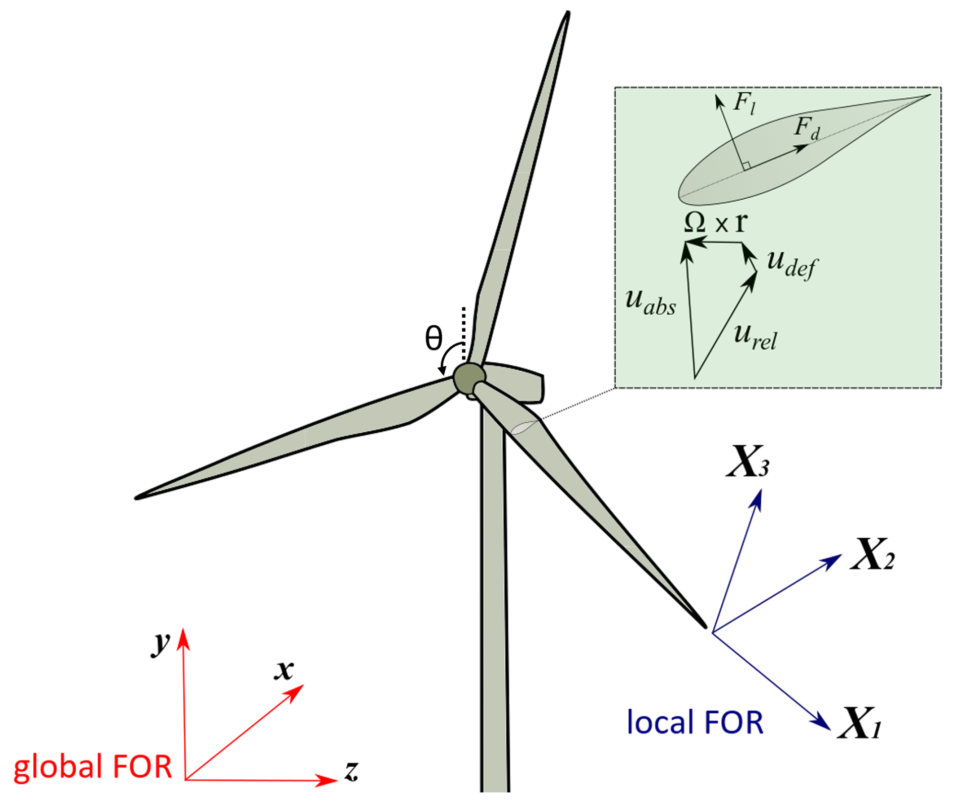
Under the assumption of linearity, the elastic generalized displacement d = (di,θi), which includes translational di and rotational θi (with i = ) degrees of freedom (DoFs), is decomposed along the coordinate X1 on the neutral axis as follows:
where ψm(X1) is the mth elastic mode shape from the modal analysis of the structure, qm is the corresponding modal coordinate, and M is the number of modes used.
The effect of the generic motion of the FOR on the relative structural dynamics (one-way inertial coupling since we assumed that the blade deformation does not modify the rotor inertia) is included on a modal basis by means of the methodology introduced in Reschke (2005) and further developed for the case of wind energy in Della Posta et al. (2022). Through this method, which exploits the decomposition of the acceleration in a moving FOR in the virtual-work principle, we obtained a system of elastic equations with additional stiffening, damping, and loading terms depending on the angular velocity and acceleration of the rotating FOR as follows:
where M, D, and K denote the modal structural mass, damping, and stiffness matrices, respectively, and e denotes the external loads expressed on a modal basis, including the gravity force acting on the local center of mass and the ALM aerodynamic forces acting on the local quarter of the chord. The remaining terms are inherently related to the various contributions to the acceleration in a moving FOR. Terms with the superscripts Co, c, and Eu are related to the Coriolis, centrifugal, and Euler accelerations, respectively. Given the assumption of linearity, we apply all the forces to the reference undeformed configuration. The discrete evaluation of the additional inertial terms in Eq. (6) is expressed as a function only of the information known from the structural finite-element method (FEM) model and from the corresponding mode shapes according to Saltari et al. (2017). For the modal analysis, performed on the undeformed non-rotating blade, we use a finite-element model of the blade based on complete beam elements with 6 DoFs, with Euler–Bernoulli behavior for bending in directions X2 and X3, and linear shape functions for axial and torsional deformations. We assume a lumped-mass representation, and we take into account the local offset of the centers of mass with respect to X1. Finally, the structural matrices are assembled considering the local twist. The generalized-α method (Chung and Hulbert, 1993) is employed to advance the structural dynamic equation in time, which is unconditionally stable for linear problems and is second-order accurate. Details about the modal analysis are provided in Appendix A.
2.1.3 Fluid–structure interaction model
The two-way coupling aeroelastic model employs the ALM sectional approach, whereby the angle of attack (AoA) and relative velocity are locally modified following the instantaneous blade motion provided by the structural dynamics. In particular, the distribution of the AoA along each blade is evaluated as a function of the velocity of the fluid, the angular velocity of the rotor, and the instantaneous elastic state of the blade (which is projected back to the physical space from the modal one once the displacement is determined). The latter is generally constructed from the deformation velocity udef = considering the time derivative of the translational degrees of freedom only and the local vector of the deformation angles θ (torsion and in- and out-of-plane angular deformations) derived from the structural solver, which is forced by the updated aerodynamic loads. The algorithm restricts inter-field communications solely at the beginning of each RK sub-step, thereby ensuring optimal computational efficiency. The impact of the torsional dynamics was deemed to be limited in light of the results obtained in previous studies on the effect of torsion for smaller wind turbines (Chen, 2017). In order to investigate this issue for the large-rotor 15 MW wind turbine, in this study, we compare two different CSD models. In particular, we consider as a baseline a two-way coupling that includes the effect of blade deformation velocity as a sole variable (CFD–CSD/OV, for only velocity) and a more complete model including the torsional deformation in the coupling (CFD–CSD/T, for torsional). In general, the relative velocity for a rotating blade can be defined with the following expression:
where uabs is the filtered velocity from the fluid solver at the actuator line, rOP is the general radial vector pointing to the considered section, Ω is the rotor rotational speed, and udef is the deformation velocity of the structure at the same position. As a result, the AoA used to determine the air load coefficients is defined as follows:
where ϕ is the local twist angle of the blade; θtors is the local torsional deformation; Ei denotes the unit vectors of the relative FOR rotating with the structure; and, hence, v2 = udef⋅E2 is the flapwise deformation velocity component, and v3 = udef⋅E3 is the edgewise deformation velocity component. The simplified coupling procedure benefits from the sectional one-dimensional formulation of the ALM, which avoids the complex treatment of the fluid–solid interface with the associated kinematic and traction conditions.
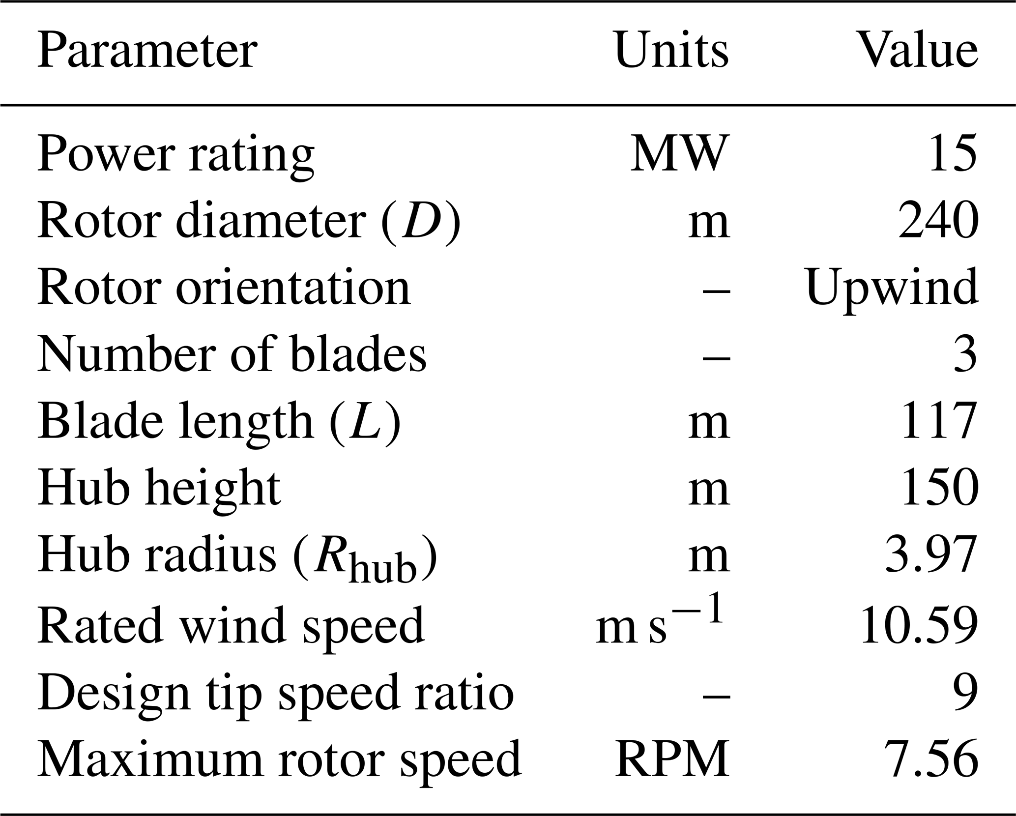
In this work, we consider a stand-alone IEA 15 MW wind turbine (Gaertner et al., 2020b) in its monopile configuration. This wind turbine has a rotor diameter D = 240 m with three blades of length L = 117 m. Table 1 provides the main features of the turbine.
Table 1IEA 15 MW (Gaertner et al., 2020b) wind turbine main features.
The computational domain has dimensions of 12.5 × 5 × 3 diameter units, as shown in Fig. 2. The distance of the turbine from the inlet of the computational domain (equal to 4 D) has been determined on the basis of the reference data available in the literature, which vary in the range of 2–5 D. Smaller distances from the inlet (2 D) have been employed for experimental setup (Bartl and Satran, 2017; Krogstad et al., 2015), whereas larger distances (in the range of 2.7–5 D) are typical of numerical simulations (Porte-Agel and Wu, 2011; Ciri et al., 2017; Allah and Sha ei Mayam, 2017; Stevens et al., 2018). Moreover, we have verified numerically that pressure fluctuations do not generate spurious reflections at the inlet section in our simulations. The spanwise length of the computational domain (equal to 3 D) is the same as that employed in previous numerical simulations (Ciri et al., 2017; Allah and Sha ei Mayam, 2017). We have verified that, using periodic boundary conditions, the blockage effect on the single turbine is negligible. Moreover, following the convergence study reported in Appendix A, the computational box has been discretized by a staggered grid composed of 2049 × 513 × 513 points in the streamwise, wall-normal, and spanwise directions, respectively. The orthogonal grid is equally spaced in the streamwise and spanwise directions and is stretched vertically, with a gradually wider spacing starting from the region above the rotor. The grid spacing described leads to an actuator line discretized by 86 points per blade. The time resolution of the LES computation is tied to the spatial resolution, as defined by the stability requirements of the numerical scheme adopted. Simulations are carried out at a constant Courant–Friedrichs–Lewy (CFL) number (Courant et al., 1967) of CFL = 0.65, which ensures an average time step of = 0.024 s. The turbine location is 4 diameter units from the inlet and is centered in the spanwise direction. Furthermore, we impose a sheared laminar inflow velocity profile, defined by a power-law with the exponent α = 0.05, and a convective outlet boundary condition, i.e., = 0, with the constant C set to the average value of the outflow velocity. Notice that, as the shear is imposed at the inlet, the flow profile is allowed to change when reaching the turbine. However, since the power-law profile complies with the no-slip conditions at the wall and with the slip conditions at the free stream, the modifications are mostly due to the slight three-dimensionalization of the flow due to the presence of the turbine. In the spanwise direction, periodic boundary conditions are imposed. Moreover, slip and no-slip conditions are enforced at the top and bottom boundaries, respectively. The turbine is subjected to a flow with a Reynolds number Re≈108 and operates at its nominal tip speed ratio (TSR) of λ=9. The streamwise undisturbed velocity at the hub height is constant and equal to U∞ = 10 m s−1. The simulations were conducted for a time interval of 300 s over the initial transient, which corresponds to 35 revolutions of the rotor.
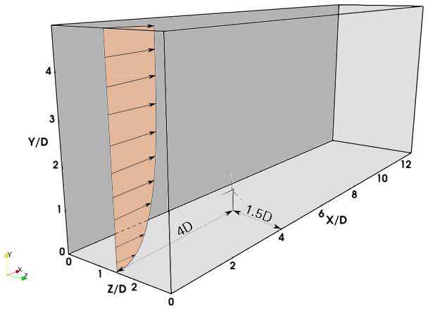
Figure 2Sketch of the computational domain where the incoming sheared flow and the position of the turbine are highlighted.
To identify the optimal configuration for the structural model, we conducted a preliminary sensitivity analysis and then validated the structural eigenfrequencies of the undeformed non-rotating blade with the results found in the literature. A more detailed insight into this analysis is presented in Appendix B, where the structural properties of this turbine are shown. Finally, a number of modes Ms = 15 and a structural discretization of the blades given by N =80 equally spaced nodes were chosen.
For comparison purposes, wind turbine simulations have also been conducted using the OpenFAST solver Release v3.2.0 (29 July 2022). The aerodynamic computations are performed by the AeroDyn (Jonkman et al., 2015) module, which is based on the BEM theory. A Prandtl loss model is applied to account for the tip and root effects. The structural module dedicated to the computation of the blade deformation is contained in the BeamDyn module, which relies on the geometrically exact beam theory and may resolve geometric non-linearities and large deflections (Wang et al., 2016b). In order to compare the CFD–CSD results with a modal structural analysis, we also performed simulations using the standalone ElastoDyn module based on a modal approach and suitable for blade deformation dominated by bending. It is worthwhile to notice that the latter does not take into account the torsional degree of freedom, and so it is to be directly compared to the CFD–CSD/OV model, which also does not account for the coupling between the torsional deformation and the angle of attack. As reported in the original manual of AeroDyn (Moriarty and Hansen, 2005), OpenFAST couples the fluid and structural solvers in a similar way to our CFD–CSD solvers. In particular, the local angle of attack is determined, taking into account the local deformation velocities.
This section presents the results of two sets of simulations: one modeling a rotor-only configuration (RO) and the other including the tower and nacelle (TN). Furthermore, both configurations are subjected to comparative analysis using the OpenFAST submodules. Firstly, the near-wake aerodynamic characteristics and the wake recovery of both configurations determined by the CFD–CSD solvers are discussed. Then, the aerodynamic loads on the blades are analyzed, and the outcomes from both solvers are compared. Finally, the overall turbine performance and the effects on the blade deformation are assessed.
4.1 Flow analysis
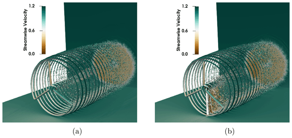
As a first step, we analyze the flow field variables, as obtained using the CFD–CSD/T solver. Figure 3 illustrates the main coherent flow structures in the field by means of an instantaneous isosurface of the Q-criterion colored by the streamwise velocity for both cases. It is evident that the presence of the tower affects the vorticity intensity distribution along the vertical direction. In particular, the occurrence of a low-velocity recirculation zone at the tower height for the TN case can be identified, which is a result of the tower shadowing (see Fig. 3b). Moreover, the TN case demonstrates a more rapid dissolution of the endogenous coherent hub vortex structures if compared to the RO case (see Fig. 3a). On the other hand, the tip vortex structures appear to be minimally influenced by the presence of the tower. Figure 4 shows the rotor-averaged streamwise velocity along the flow direction, time-averaged over 30 revolutions of the rotor. Contrarily to what Santoni et al. (2017) observed in their work on the 5 MW reference turbine invested by a uniform inflow (see the red lines in Fig. 4), the rotor-averaged velocity for the TN configuration in the wake remains slightly lower than for the RO case, indicating that wake recovery is slightly hindered by the presence of the tower. In order to establish whether this opposed behavior with respect to the results of Santoni et al. (2017) may be due to the different inflow or rather geometrical features characterizing the two different turbines, we have carried out a computation equivalent to that of the 15 MW turbine (sheared inflow, U∞ = 10 m s−1 etc.), but for an NREL 5 MW wind turbine. As shown by the blue lines in Fig. 4, as in Santoni et al. (2017), the rotor-averaged velocity for the TN configuration in the wake remains somewhat higher than for the OR case, indicating that wake recovery for an NREL 5 MW turbine is indeed advanced by the presence of the tower, no matter the inflow considered. On the other hand, the larger gap between the RO and TN cases observed in the near wake by Santoni et al. (2017) is not observed in this case, and it is thus probably due to the uniform inflow. Comparing these results to the present data, we can conclude that the slower wake recovery observed for the 15 MW turbine in the presence of the tower appears to be due to geometrical features of the turbine itself and not due to the inflow characteristics. One possible explanation for this behavior could be differences in the tower-to-rotor aspect ratio. In particular, for the NREL 5 MW turbine, the ratio between the tower diameter and the rotor diameter is about equal to 0.047, whereas, for the 15 MW turbine, it is only about 0.027 (the tower diameters being 6 and 6.5 m, respectively). Thus, the thinner shape (in terms of diameter units) of the tower and the lower value of the incoming velocity at the tower height due to the presence of shear at the inflow result in a decreased mixing behind the turbine, which leads to a slower wake recovery.
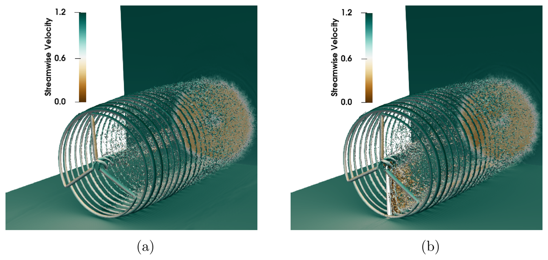
Figure 3Q-criterion contour of the instantaneous velocity field colored by the streamwise velocity for the rotor-only case (RO) (a) and the tower and nacelle (TN) (b).
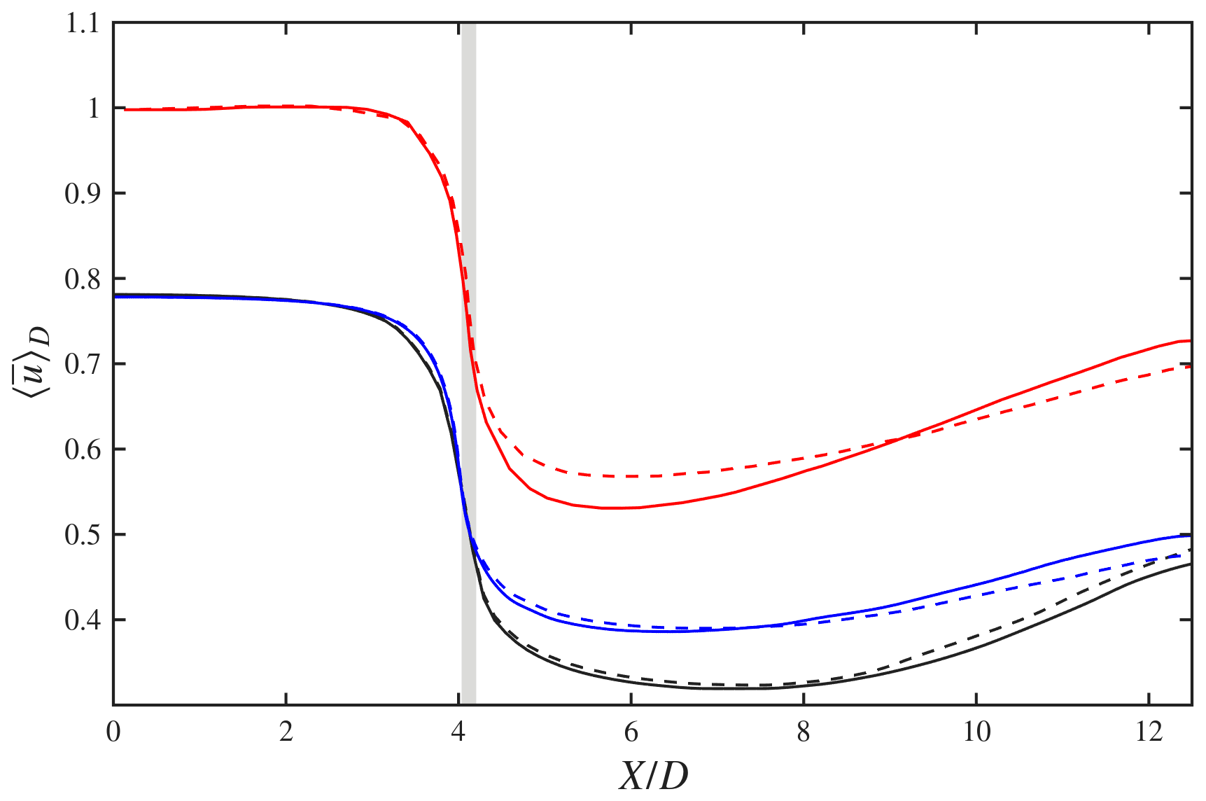
Figure 4Rotor-averaged velocity along the streamwise direction normalized by the undisturbed velocity at the rotor height, namely, U∞ = 10 m s−1, for the present data (black curves), a computation of the NREL 5 MW turbine for the same configuration and inflow (blue curves), and the work of Santoni et al. (2017) (red curves). The gray region represents the area covered by the rotor (RO – dashed line; TN – solid line).
Although not favoring wake recovery, the tower still plays a strong role in the wake dynamics, as can be visualized in Fig. 5, showing slices of instantaneous streamwise velocity at different tower heights corresponding to 80 % of the blade (top) and to the tip of the blade (bottom) when the blade is in front of the tower, i.e., θ = 180° (left), and when it is far from it (right). In particular, it can be observed that the turbulent mixing right downstream of the tower is already very high in the near wake compared to that close to the tip of the blades. Due to the mutual effect of the asymmetry induced by the rotation of the blades and of the wake meandering, it can be seen that, inside the rotor disk, the tower wake bends in the spanwise direction (Fig. 5, top frames), whereas it is rather spanwise independent at a height corresponding to the blade's tip (bottom frames). Moreover, one can see that the passage of the blade in front of the tower (left frames) already induces a strong perturbation in the flow field upstream of the tower. In the following section, the effect of this perturbation on the phase oscillations of several relevant quantities (aerodynamic forces, power coefficient, etc.) will be discussed.
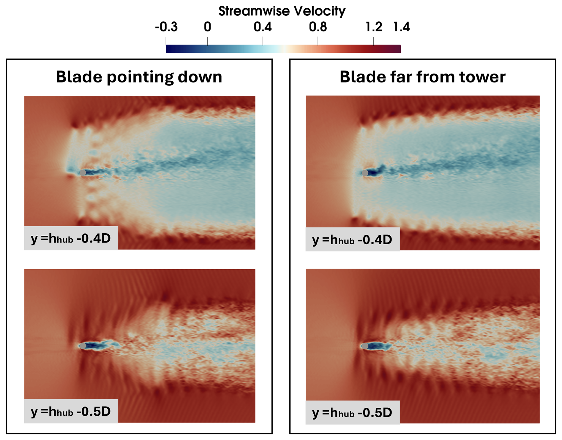
Figure 5Instantaneous streamwise velocity on horizontal slices at different tower heights corresponding to 80 % of the blade (top slices) and the tip of the blade (bottom slices). In the left configuration, the blade is in front of the tower (θ = 180°), while, on the right, the blade is far from the tower. hhub = 0.625 D is the hub height.
4.2 Aerodynamic loads on the blade
The analysis of the aerodynamic loads on the blade has been conducted using the present CFD–CSD models and the engineering software OpenFAST. The same laminar sheared inflow is imposed for both solvers using a power-law with the same exponent and reference streamwise velocity at the hub height. We have chosen not to impose a turbulent inflow to avoid differences in the definition of the turbulent inflow itself, which might have hindered the comparison between the results of the two codes. It is important to note that the four solvers employed differ in terms of both their aerodynamic and structural modeling approaches. Moreover, the flow that impacts the turbine is not exactly the same for the CFD and OpenFAST solvers since, in the former case, it is imposed at several diameters upstream the rotor plane. As a result, it is not always possible to unambiguously determine whether the observed discrepancies in the results originate from the fluid–dynamic models or from the structural formulations.
Figure 6 depicts the following time-averaged aerodynamic quantities along the span of the blade: the local angle of attack α (Fig. 6a); the aerodynamic pitching moment per unit length Maero (Fig. 6b); and the flapwise and edgewise components (normal and tangential to the rotor disk, respectively) of the aerodynamic force per unit length F2 (Fig. 6) and F3 (Fig. 6d), respectively. In particular, Fig. 6a shows that a good agreement of the local incidence angle computed by both CFD–CSD models (solid lines) with that computed by ElastoDyn (circles) and BeamDyn (squares) is obtained from 20 % and up to 80 % of the blade length. Indeed, the differences in the root area could be ascribable to the presence of the hub, which is modeled differently by the solvers. The discrepancy of the incidence angle observed towards the tip subsequently affects the aerodynamic loads. The F2 force in Fig. 6c shows a very good fit of the CFD–CSD/T results with that of the non-linear solver BeamDyn despite the linearity of our in-house CSD model. The strong discrepancies with respect to the values obtained by ElastoDyn can be ascribed to the absence of the torsional deformation in the latter solver. Indeed, the CFD–CSD/OV solver, which neglects the torsional feedback in the coupling, shows very similar results to the ElastoDyn solver. A similar effect can be observed by examining the reduction in F3 towards the tip of the blade (see Fig. 6d). The distribution of the aerodynamic pitching moment presents, instead, a maximum gap of about 8 % from the BEM-based solvers.
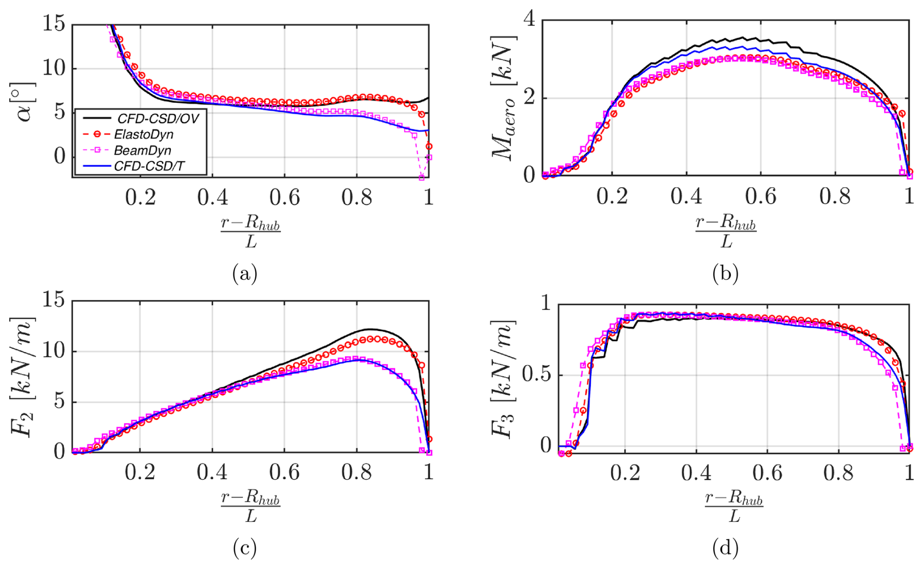
Figure 6Average aerodynamic quantities along the blade compared between CFD–CSD/OV, CFD–CSD/T, ElastoDyn, and BeamDyn. (a) Incidence angle, (b) aerodynamic pitch moment, (c) flapwise aerodynamic force, (d) edgewise aerodynamic force.
As demonstrated by Hansen (2015), the outer third of the blade span is the most critical region in terms of deflections and deformations due to the combination of higher aerodynamic loads and reduced structural stiffness. Therefore, a phase average of the aerodynamic quantities at 80 % of the blade has been performed. Figure 7 reports the evolution of the incidence angle and of the aerodynamic force components at = 0.8 (with Rhub being the hub radius and L being the blade length) versus the blade rotation angle θ. The dynamical behavior of the aerodynamic quantities in the presence (solid lines) or in the absence (dashed lines) of the tower underlines the fact that the passage of the blade in front of the tower represents the main source of instability for the flow conditions considered. Indeed, the blade–tower interaction leads to oscillations of the aerodynamic forces and of the incidence angle around θ = 180°, i.e., when the blade is pointing down. However, unlike the case of the NREL 5 MW turbine (Bernardi et al., 2023), this effect appears to be stronger for the BEM computations than for the CFD–CSD solver. Concerning this point, we should recall that, as pointed out by Bernardi et al. (2023), the complex flow dynamics resulting from the interaction between the blade and the tower, shown in Fig. 5, may not be well described by OpenFAST, which uses a simple potential flow model. It can be observed that, between the rotor and the tower, a region with low streamwise velocity is observed. We can expect that the passage of the blade in front of the tower thus induces an alteration of the aerodynamic forces on the blade due to the decrease or increase in the streamwise velocity. This issue will be further discussed in the following, where a possible reason for the different behavior observed for the IEA 15 MW with respect to the NREL 5 MW turbine will be discussed.
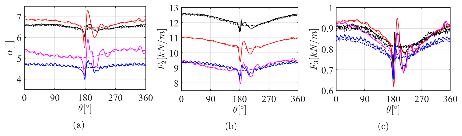
Figure 7Phase-averaged values of (a) the local incidence angle, (b) flapwise aerodynamic force, and (c) edgewise aerodynamic force at 80 % of the blade. CFD–CSD/OV: TN (solid black line), RO (dashed black line). CFD–CSD/T: TN (solid blue line), RO (dashed blue line). ElastoDyn: TN (solid red line), RO (dashed red line). BeamDyn: TN (solid magenta line), RO (dashed magenta line).
Apart from the effect of the tower, one can observe a rather good match between the CFD–CSD/OV and ElastoDyn solvers for both the incidence angle and the edgewise component of the aerodynamic force, while the flapwise component presents some discrepancies. On the other hand, when torsional feedback is included, CFD–CSD/T and BeamDyn solvers, regardless of the linearity or non-linearity of the models, agree rather well with regard to the aerodynamic forces, especially the flapwise one, which shows an error of ≈ 2 %, while the edgewise force reaches an error of ≈ 5 % at azimuthal angles close to θ = 0. On the other hand, the error between the two solvers on the angle of attack reaches 8 %.
To better investigate the local response of the different models during the blade revolution, we conducted a comparative analysis of the aerodynamic loads, employing phase-averaged quantities over the span. Figure 8 illustrates the percentage difference of the phase-averaged aerodynamic quantities on the rotor plane of the ElastoDyn (BeamDyn) solver with respect to the CFD–CSD/OV, defined as , and of the CFD–CSD/T model, defined as , respectively. In particular, in comparison to ElastoDyn, a higher value of the absolute incidence angle in the range of = [17 %,25 %] is found in the zone after the tower (see Fig. 8a). The difference with respect to the results obtained by BeamDyn tends to be higher when moving from the root to the tip, with a discontinuity in the tower area, spanning the range = [35 %,60 %] in the last 20 % of the blade span. Furthermore, the angle-of-attack distribution affects the components of the aerodynamic force. In fact, the distribution of the flapwise component of the force follows the same pattern of the incidence angle (see Fig. 8b). On the other hand, for the edgewise component, the major discrepancies are concentrated in the final radial sections of the blade towards the tip (see Fig. 8c). In general, we can conclude that the most significant discrepancies are observed in the tip region, where the three-dimensional effects are more relevant and where the complexity of the fluid flow is strongly affected by the presence of the tower.
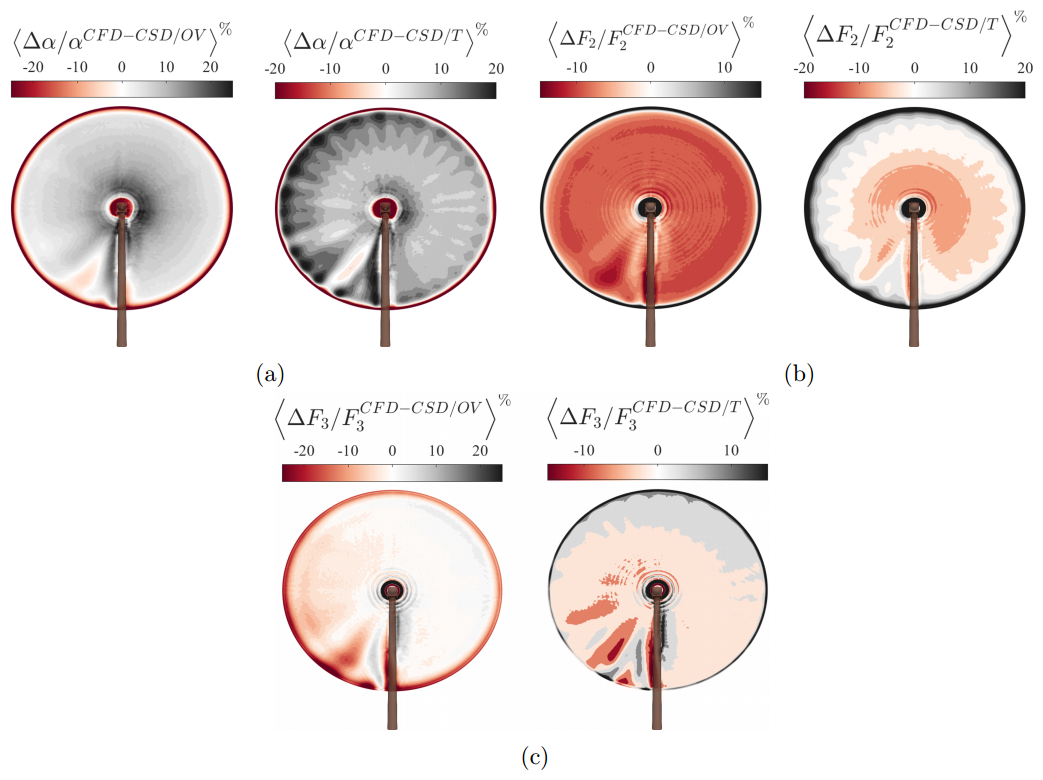
Figure 8Phase-averaged contour plots of the percentage differences of the aerodynamic quantities between CFD–CSD/OV versus ElastoDyn (left) and CFD–CSD/T versus BeamDyn (right). (a) Incidence angle, (b) flapwise aerodynamic force, (c) edgewise aerodynamic force.
Notably, similar discrepancies are observed when comparing the CFD–CSD/T solver with the BeamDyn solvers. However, in this case some high-frequency oscillations are observed for the three aerodynamic quantities. In fact, the same oscillations are observed in the phase averaged quantities at 80 % of the blade shown in Fig. 8, for both the CFD–CSD/T solver and BeamDyn. The frequencies of these oscillations computed by the two solvers appear to be very close and comparable with the natural frequency of the first torsional mode, although some differences can be observed in the amplitudes of the signals, especially concerning the angle of attack (≈ 8 % of error) and the edgewise aerodynamic force at azimuthal angles close to zero (≈ 6 % of error). Again, this observation indicates that including the torsional degree of freedom in the structural solver is crucial for describing accurately the amplitude and dynamical behavior of the aerodynamic quantities.
4.3 Power and thrust coefficients
The aerodynamic loads previously presented are also useful to evaluate the power and thrust coefficients, defined as follows:
where A = represents the rotor area, Pd is the aerodynamic power transferred to the rotor, and Taero is the overall aerodynamic thrust on the turbine.
Starting from the time history of Cp and Ct, we computed their phase-averaged evolution as reported in Fig. 9. The periodic passage of the blades in front of the tower for the TN configuration produces a drop in the curves of about 10 %. Eventually, the performance is restored to the value obtained in the RO case following the elastic dynamical behavior of the structure. The results reflect the dependency of the power and thrust coefficients on the edgewise aerodynamic force F3 and the flapwise aerodynamic force F2 at 80 % of the blade, respectively (see Fig. 6c and b), which are strongly influenced by the presence of the tower. Notice that, here, we can also observe that the drop in the Cp curve appears to be rather similarly predicted by BEM and CFD, although the BEM prediction exhibits notable oscillations before and after the drop, whereas these are not present in the CFD results. A different behavior was observed for the NREL 5 MW turbine (as in Fig. 3 of Bernardi et al., 2023, included in Fig. 9 of the present paper with symbols), where this performance drop is considerably underestimated by the BEM computations. A possible factor that may contribute to this different behavior may reside in the different relative geometry of the two wind turbines. Indeed, the flow induced by a thinner tower (in diameter units), as in the case of the 15 MW wind turbine, might be better described by a potential flow solution compared to the one induced by a thicker tower, as in the case of the 5 MW wind turbine, and may thus lead to the observed improved agreement between BEM and CFD results. Moreover, the differences in the flow impinging on the blade might also have an effect. In fact, in Bernardi et al. (2023), a uniform inflow was imposed. On the other hand, in the present case, due to the shear imposed at the inflow and the limited distance from the ground of the tip of the blade (only ≈0.125 D for the 15 MW turbine), the blade is invested by a flow with a much smaller velocity compared to the given value of U∞ at hub height, further confirming the increased suitability of a potential flow solution upstream of the tower. Nevertheless, we should recall that this remains a very strong approximation, as also demonstrated by the differences in the forces and angles that have been observed in the previous section (see Fig. 8, for instance).
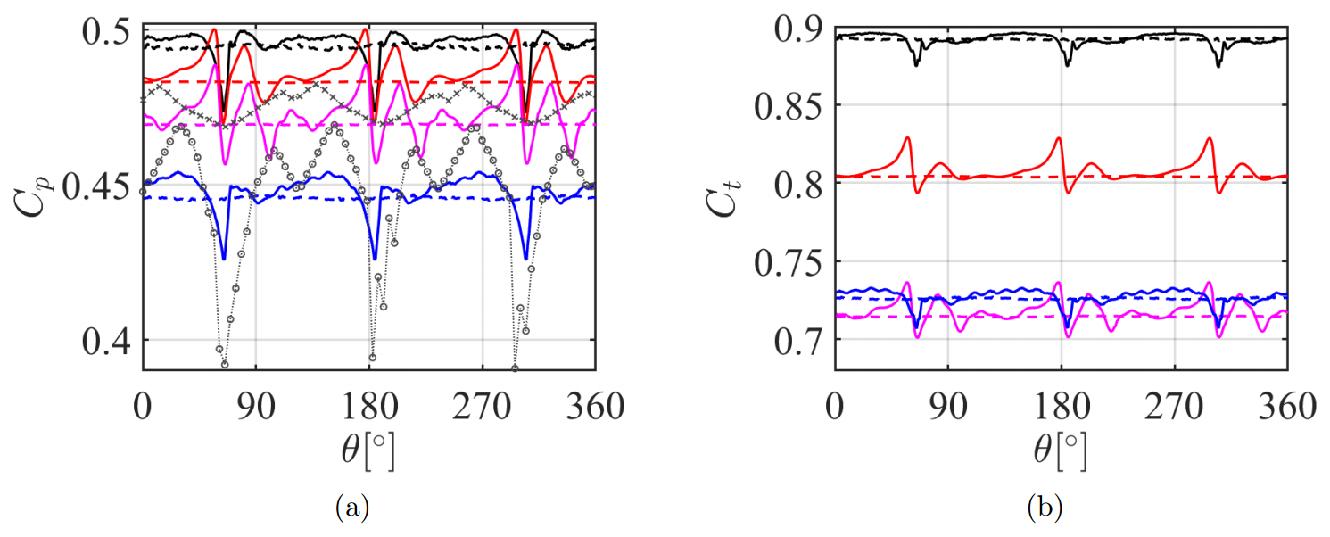
Figure 9Phase-averaged power (a) and thrust (b) coefficients. CFD–CSD/OV: TN (solid black line), RO (dashed black line). CFD–CSD/T: TN (solid blue line), RO (dashed blue line). ElastoDyn: TN (solid red line), RO (dashed red line). BeamDyn: TN (solid magenta line), RO (dashed magenta line). From Fig. 3 of Bernardi et al. (2023): LES + CSD flexible (circular gray markers), OpenFAST-AeroDyn (gray cross markers).
It can be concluded that the performance loss induced by the passage in front of the tower is less pronounced for the 15 MW NREL turbine in the present configuration (≈ 5 %) compared to for the 5 MW turbine in the configuration considered in Bernardi et al. (2023) (≈ 15 %; see Fig. 3 of this reference), with both BEM theory and CFD yielding similar predictions in the case of the 15 MW turbine. However, it is worth recalling again that Bernardi et al. (2023) considered a uniform inflow, whereas, here, the inflow is sheared. This could be a possible reason for this different behavior since the lower wind speed in the lower part of the rotor plane leads to a lower production in the bottom half of the rotor plane, where the tower is located. This may cause a smaller performance drop due to the tower relative to the total produced power. Therefore, the observed difference can be due to not only the change in turbine size but also the change in inflow conditions.
Moreover, the present results predict that, for very large rotors and a sheared inflow, the tower effect on blade deformations is less pronounced than for smaller rotors, although it should yet be taken into account for accurately describing the turbine's performance oscillations as it still represents a major source of unsteadiness.
The average value of the power coefficient is much larger when the torsional deformation is neglected. This feature is observed by both CFD and BEM approaches. However, one can observe that ElastoDyn underestimates the value of Cp with respect to the corresponding non-torsional CFD model, while the opposite is observed when comparing BeamDyn with the torsional CFD solver. This is probably due to the fact that BeamDyn predicts higher values of the aerodynamic edgewise forces with respect to the CFD–CSD/T approach, which are linked to a smaller torsional deformation, as will be shown in Fig. 11f in the next section.
Figure 10 shows the premultiplied power spectral density (PSD) of the power (Fig. 10a) and thrust (Fig. 10b) coefficients' evolution. The PSD is normalized by the variance of each coefficient σ2 and plotted versus the frequency normalized by the rotational frequency of the rotor , where the latter is denoted as 1P = frot = 7.5 RPM, and its multiples will be denoted as 2P, 3P, etc. In both cases, the CFD–CSD solvers seem to provide a richer representation of the aerodynamic coefficients, capturing the full range of flow–structure interactions. Indeed, an examination of the low-frequency behavior reveals that both quantities exhibit isolated low-frequency peaks when using the BEM-based solvers, a phenomenon not observed with the CFD–CSD, where the low-frequency range is rather broadband and does not present particular peaks. It is important to notice that the frequency 1P can be directly linked to the frequency of the passage of the blade in front of the tower but also to wind shear loads on the blades. Concerning the first point, a potential flow solution such as that used in the BEM solver is likely to provide a simple, single-frequency response, whereas a complex, turbulent flow is expected to result in a more broadband spectrum. Concerning the second point, we have to consider that, in LES, the power-law profile is imposed at the inlet of the domain, but it is free to evolve for 4 diameters before the wind turbine, altering in a non-trivial way the flow field and the consequent frequency response of the blades. This outcome indicates that the BEM-based solvers tend to overcut the power oscillations associated with low frequencies that are not exactly equal to 1P or 2P. For all solvers, however, the strongest PSD peaks are to be found at much larger frequencies (3P-6P-9P-12P), as also observed by Pagamonci et al. (2023) by means of URANS aeroelastic simulations of the NREL 5 MW, the DTU 10 MW, and the IEA 15 MW turbines. One can also notice that the amplitude associated with the 3P frequency appears to be consistently described by the two solvers, although, in this range, the BEM solver also appears to overdamp the frequencies in between different peaks. Moreover, a good agreement is evident between the two sets of results with regard to the value of the frequencies and the level of the PSD for frequencies that are multiples of 3P.
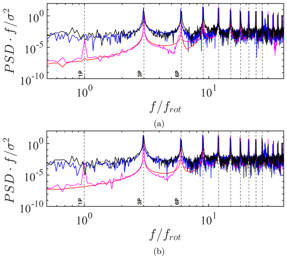
Figure 10Power spectral density (PSD) of the power (a) and thrust (b) coefficients. The vertical dashed lines highlight the rotational frequency of the rotor 1P = frot = 7.5 RPM and the multiples of 3P, respectively. CFD–CSD/OV (black line), CFD–CSD/T (blue line), ElastoDyn (red line), and BeamDyn (magenta line).
4.4 Structural response
This section presents the analysis of the structural dynamics. Figure 11 reports the phase-averaged dynamic response of the free extremity of the blade (left column) and the time-averaged deformation of the entire span (right column). Figure 11a shows how the out-of-plane deformation is mainly governed by the aerodynamic component of the force normal to the rotor plane and, hence, to the aerodynamic effects, heavily affected by the tower. In fact, it is visible how the tower placed at θ = 180° produces a drop in the deformation, followed by an elastic dynamic response which restores the value far from the pointing-down position. The time-averaged maximum deformation predicted by the CFD–CSD/OV solver is 16 % higher compared to the ElastoDyn module and 17 % higher compared to BeamDyn (see Fig. 11b). On the other hand, the same quantity predicted by the CFD–CSD/T solver is 17 % lower compared to the ElastoDyn module and 13 % lower compared to BeamDyn (see Fig. 11b). This is consistent with the fact that including the torsional degree of freedom reduces the loads (see Fig. 6b) and the resulting deformation. Although the trend of deformation with respect to the blade span appears to be similar to previous predictions based on URANS (see Pagamonci et al., 2023), the out-of-plane deformation is somewhat larger, reaching 16 m at the blade's tip. The amplitude of the deformation is, however, close to that obtained by Trigaux et al. (2024) using LES. Figure 11c depicts instead the in-plane deformation, which is mostly due to gravity. The results show that the shadowing effect of the tower does not influence this quantity, which is expected as the lag deformation is mainly driven by gravity. Furthermore, the discrepancies obtained between ElastoDyn and BeamDyn can be attributed to the lack of modes used by the former model to describe the translation in the edgewise direction (see Fig. 11d). The discrepancy does not seem to be linked to the linearity of this model as the result of the CFD–CSD/T solver, which is linear as well, is much closer to the BeamDyn results. Moreover, the results of the CFD–CSD/OV and the CFD–CSD/T models are very close each other. It can be noticed that the amplitude of the oscillation of the in-plane deflection is consistent with that reported by Trigaux et al. (2024) (see Fig. 7b of their paper, reporting an oscillation between ≈ −2.3 and ≈ 0.2), although the sign is opposite due to the different frame of reference used.
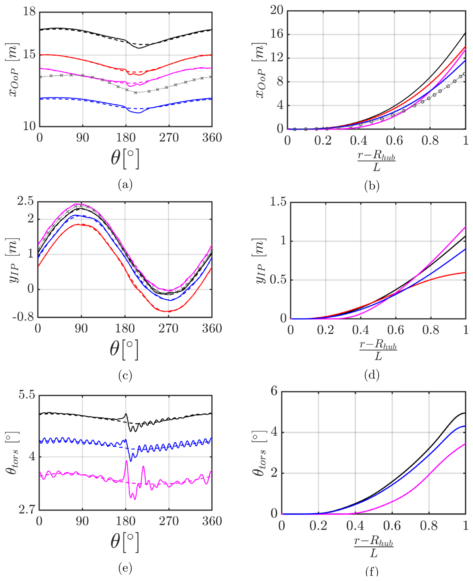
Figure 11Phase-averaged deflections at the tip of the blade (a, c, e) and time-averaged deflections along the blade span (b, d, f). CFD–CSD/OV: TN (solid black line), RO (dashed black line). CFD–CSD/T: TN (solid blue line), RO (dashed blue line). ElastoDyn: TN (solid red line), RO (dashed red line). BeamDyn: TN (solid magenta line), RO (dashed magenta line). From Fig. 13 of Pagamonci et al. (2023) (circular gray markers) and Fig. 7a and b of Trigaux et al. (2024) (gray cross markers).
A further significant insight into the deformation phenomenon is provided by the torsional DoF. Figure 11e shows a comparison of the torsional angle at the tip with BeamDyn. Significant discrepancies can be observed between the LES and the BEM approaches, which cannot be reconducted to the different coupling procedures adopted by the models. On the one hand, BeamDyn and CFD–CSD/T both take into account the deformation angle in the coupling (Wang et al., 2016b), while, in the CFD–CSD/OV solver, the angle of attack depends only on the deformation velocity (see Eq. 8). However, the gap between the BEM and the CFD–CSD/T curves is quite large, reaching approximatively 20 % of the torsional deformation value. These differences likely arise from the combined effects of both aerodynamic and structural modeling approaches used in BEM and LES. Although in the present paper we have mostly focused on a comparison of the structural models, a thorough comparison of the aerodynamics modeling can be found in the report of IEA Task 47 (Schepers et al., 2025), where results produced with the present code are included (see, for instance, Fig. 4.25, 4.26, and 4.27 for non-flexible blades). The discrepancy between the BEM and the CFD–CSD results is confirmed by the time-averaged torsional deformation along the span reported in Fig. 11f, where the maximum percentage gap of BeamDyn reaches 29 % for the CSD-CFD/OV and 24 % for the CFD–CSD/T. It is noteworthy that the lower torsional deformation resulting from BeamDyn leads to the higher aerodynamic loads observed in Fig. 6c.
Finally, Fig. 12 illustrates the power spectral density (PSD) of the blade's tip deformation components for the TN configuration (which is characterized by more complex fluid–structure interactions). The premultiplied PSD values are normalized by the variance of the signal, σ2, and plotted versus the frequency normalized by the rotor frequency, . Spectral results have been corroborated through use of the Welch and Lomb–Scargle PSD estimation algorithms.
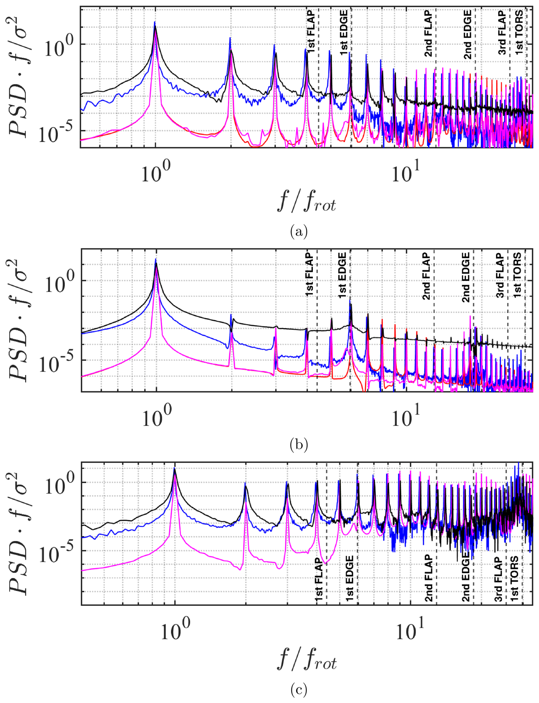
Figure 12Power spectral density (PSD) of the out-of-plane (XOoP) (a), in-plane (yIP) (b), and torsional (θtors) (c) deformations of the blade. The vertical dashed lines represent the first eight eigenfrequencies of the system. CFD–CSD/OV (black line), CFD–CSD/T (blue line), ElastoDyn (red line), BeamDyn (magenta line).
Figure 12a shows the out-of-plane deformation, which we showed to be influenced mostly by the aerodynamic loading. The results indicate that, for all of the numerical approaches used, the observed structural response does not exhibit a peak corresponding to the first flapwise natural frequency, suggesting that the intrinsic dynamics of the structure might play a less prominent role in the deformation process. A similar behavior is found in the results of Trigaux et al. (2024) (see Fig. 6 of the cited paper) for the same turbine and similar inflow conditions. Noticeably, all of the numerical models recovered peaks at frequencies close to the (highly damped) second and third flapwise natural frequencies, but, rather, they appear to correspond to the 13th and 26th multiple of the rotational frequency (i.e., 13P and 26P). Both CFD–CSD solvers predict larger-amplitude responses across a broad frequency range compared to OpenFAST, indicating a higher capability to capture complex flow interactions, including turbulence-induced vibrations. This effect is particularly pronounced at the lower frequencies, probably due to the large-scale three-dimensional structure of the flow impinging on the turbine, which is not captured by OpenFAST, also due to the fact that the impinging flow on the turbine is purely two-dimensional, while it is not for CFD. For this reason, these aspects seem to be under-represented in the ElastoDyn and BeamDyn solutions. Although the ElastoDyn curve aligns with both the CFD–CSD solvers at some key frequency peaks, it does not account for the fine-scale flow–structure interactions. On the other hand, the BeamDyn curve provides better agreement with the CFD–CSD solvers, especially at higher frequencies near the blade's natural modes, suggesting that BeamDyn captures more of the structural dynamics, particularly the aeroelastic response, probably due to its non-linearity or the number of degrees of freedom considered. Figure 12b shows the in-plane deformation, which is primarily influenced by gravity, centrifugal, and Coriolis forces acting on the blade. The CFD–CSD solvers again demonstrate stronger low-frequency components.
Figure 12c presents the torsional deformation for the CFD–CSD/T and BeamDyn solvers, excluding ElastoDyn, which neglects the torsional DoFs in the model. Additionally, this quantity also demonstrates that the CFD–CSD curves predict higher amplitudes at low frequencies. However, a good agreement between the two solvers is evident at higher frequencies, especially in the range around the first torsional eigenfrequency.
This study investigated the aeroelastic response of the IEA 15 MW wind turbine by employing a high-fidelity computational fluid dynamics (CFD) solver that couples large-eddy simulation (LES) with a computational structural dynamics (CSD) solver. Two different CSD solvers are considered: the CFD–CSD/OV solver, in which the only structural quantity contributing to the definition of the angle of attack is the deformation velocity, and the CFD–CSD/T solver, in which the instantaneous torsional deformation is also considered when defining the local effective incidence. The results of the two CFD–CSD solvers are compared with those of traditional engineering solvers such as BeamDyn and ElastoDyn, both relying on blade element momentum (BEM) theory. Two case studies were examined: a rotor-only configuration (RO) and one that included the tower and nacelle (TN).
The power spectral density (PSD) of the power and thrust coefficients revealed that the CFD–CSD solver captures a broader range of flow–structure interactions, with a more broadband low-frequency response, compared to the BEM-based solvers. The isolated low-frequency peaks found in BeamDyn and ElastoDyn suggest that these solvers tend to over-simplify the aerodynamic fluctuations associated with phenomena such as wind shear and tower shadowing. For the large IEA 15 MW turbine, the performance drop caused by tower passage is not very pronounced, and the resulting oscillations predicted by the BEM approach appear to be larger than the CFD–CSD solver.
Concerning the forces on the blade and the incidence angle, one can observe a rather good match between the CFD–CSD/OV solver and ElastoDyn, as well as between the CFD–CSD/T model and the BeamDyn solver. This is likely due to the presence – or not – of the torsional feedback, while non-linearities of the structural solver appear to have only a limited impact on the observed quantities. In agreement with previous studies, the results thus suggest that including the torsional degree of freedom in the structural solver is crucial for accurately describing the amplitude and dynamical behavior of the aerodynamic quantities.
Moreover, it is observed that duly taking into account the torsional degree of freedom reduces the value of Cp. This feature is consistently observed by both CFD and BEM approaches. However, one can observe that BeamDyn predicts lower values of the torsional deformation and, thus, higher values of the aerodynamic edgewise forces with respect to the CFD–CSD/T approach, leading to a larger Cp value than that predicted by LES. All in all, it can be concluded that, for the considered setup, the CFD–CSD solvers tend to exhibit larger amplitudes at lower frequencies with respect to BEM ones.
The structural response of the wind turbine blade has been assessed by comparing the out-of-plane, in-plane, and torsional deformations obtained from the CFD–CSD solvers and the ElastoDyn-based and BeamDyn-based OpenFAST solver. In-plane deformation, influenced significantly by centrifugal forces, appears to be better captured by the CFD–CSD solvers, especially in the low-frequency range. Concerning the out-of-plane deflection, large discrepancies are seen between the two CFD–CSD solvers, as well as between both BEM modules and the LES.
Our results underscore the importance of incorporating torsional deformation effects in the definition of the angle of attack and using high-fidelity aeroelastic models to ensure accurate predictions of wind turbine blade performance with richer fluid dynamics. On the other hand, the linearity of the structural model does not appear to have a strong effect on the aerodynamical quantities, deformations, and loads. In general, the comparison of the results of the CFD–CSD solver with those of the engineering solver shows differences, especially in the region behind the tower. The observed differences likely stem from the combined effects of differences in aerodynamic and structural fidelity and cannot be uniquely attributed to one component alone.
Future work will explore the effect of turbulent fluctuations at the inlet to better investigate the impact of the atmospheric boundary layer on the aerodynamic forces, loads, and deformations of the present turbine.
A grid convergence study was conducted to evaluate the sensitivity of the LES results to spatial and temporal resolution. Two further simulations were carried out using grids of different densities: a coarser mesh and a finer mesh, having approximately 40 % fewer and more grid points than the former in each spatial direction, respectively. This allowed for a more detailed resolution of flow structures and aerodynamic quantities. Moreover, both simulations use the same CFL = 0.65 as the present grid. The average time step obtained and the other key parameters of different LES runs are summarized in Table A1.
Table A1Comparison of the main parameters for different meshes.
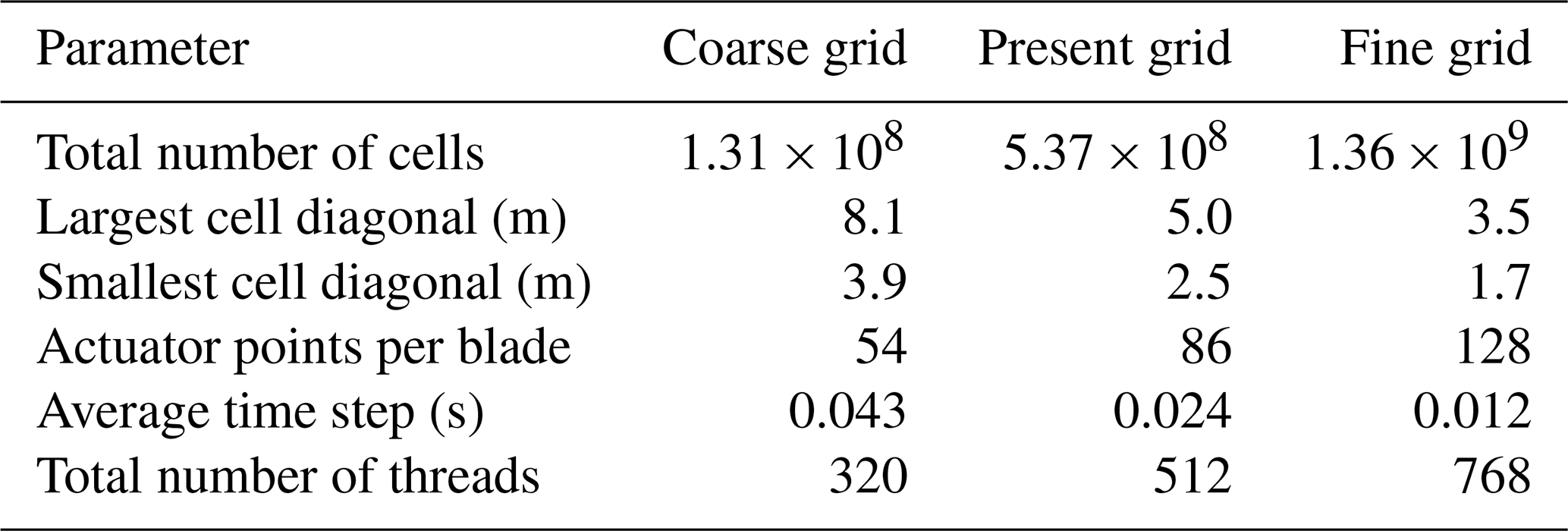
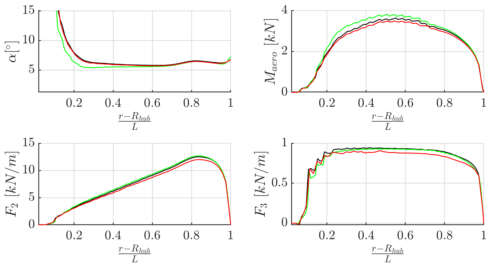
Figure A1Average aerodynamic quantities along the blade obtained from the coarse grid (red line), the present grid (black line), and the finer grid (green line). Incidence angle (top left), aerodynamic pitch moment (top right), flapwise aerodynamic force (bottom left), and edgewise aerodynamic force (bottom right).
The comparison in Fig. A1 shows that the results obtained using the coarse and fine grids are extremely close to each other along the entire blade span. In particular, the curves of the angle of attack are almost indistinguishable for the coarser and the reference grid, even in the outer portion of the blade, where stronger differences were expected due to tip effects and local three-dimensionality. Slightly larger differences are recovered between the reference and the finer grid but only with a low radius. In particular, for these two grids the maximum deviation of the incidence angle α between the two simulations at 80 % of the span reaches a value of Δαmax ≈ 0.2°, corresponding to a relative difference of 1.6 %. On the other hand, the maximum deviation between the reference and the coarser grids at 80 % of the blade span is Δαmax ≈ 0.1°, corresponding to a relative difference of 1.5 %. Similarly, the aerodynamic force component distributions exhibit negligible variation between the reference and finer resolutions and less than 1 % relative variation between the reference and the coarser grids, confirming the overall consistency of the LES solution examined in the Sect. 4 with respect to mesh refinement.
These results indicate that the coarse grid already accurately captures the main aerodynamic features, making the use of a finer mesh unjustified given its higher computational cost and minimal accuracy gain.
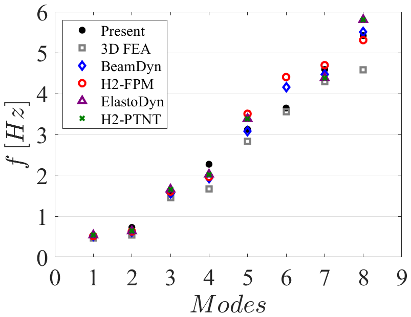
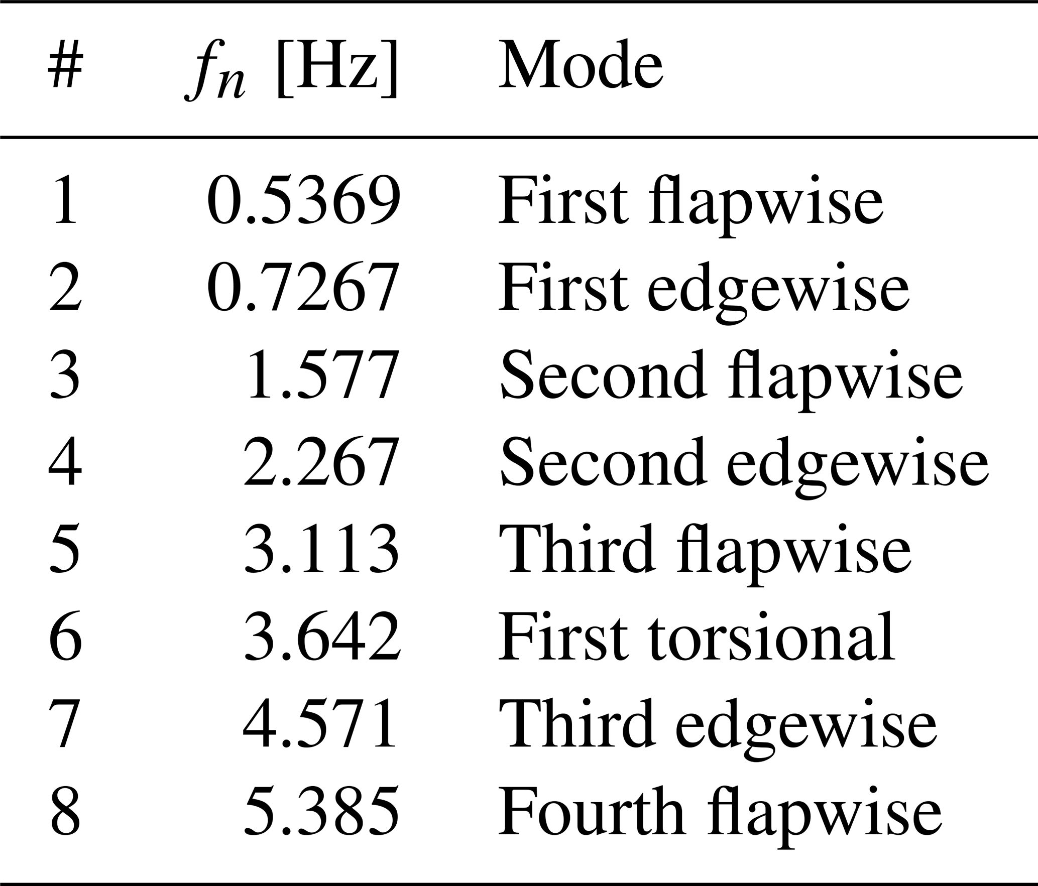
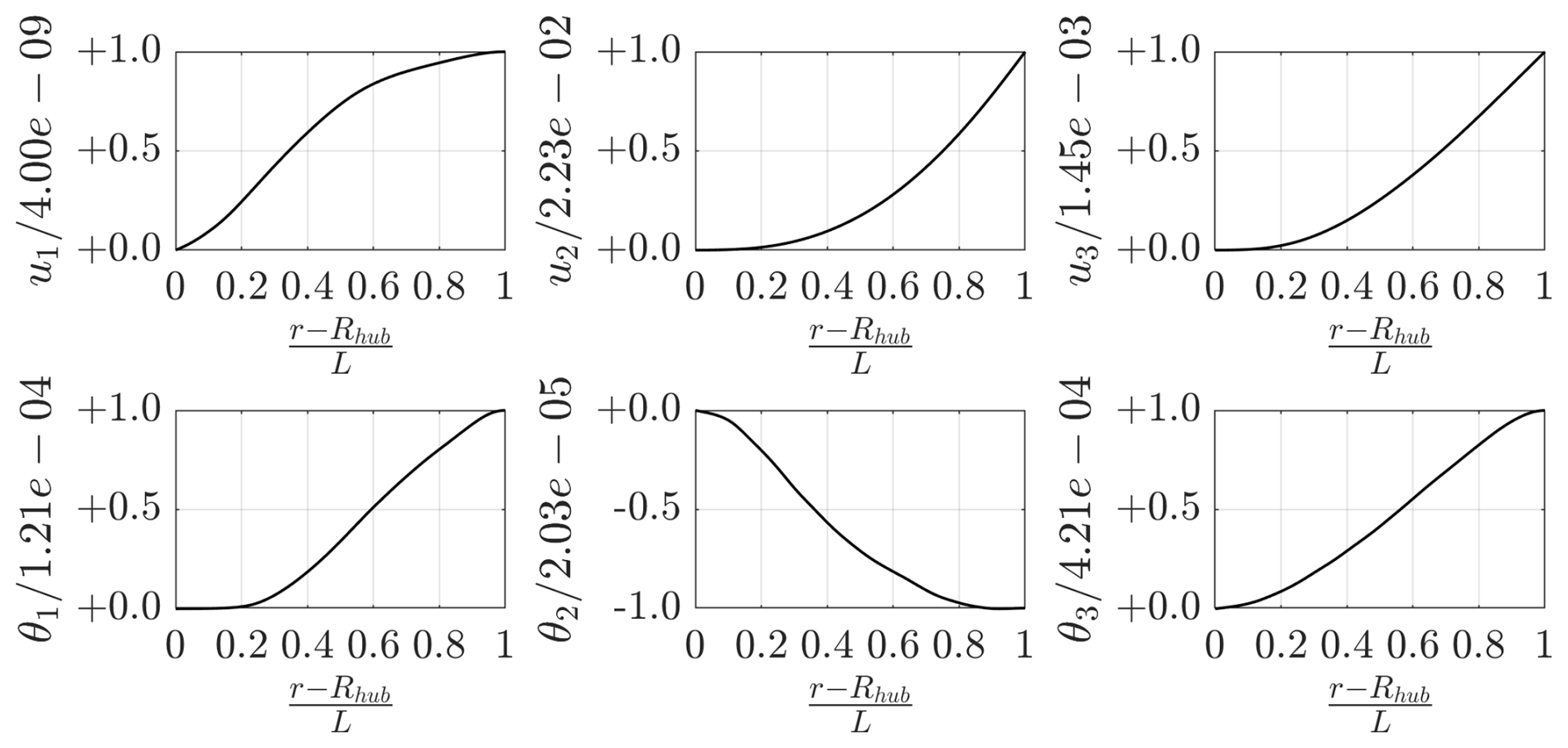
The structural model for the IEA 15 MW wind turbine has been cross-validated with many other aeroelastic numerical codes within the framework of the International Energy Agency (IEA) Wind TCP Task 47 TURBINIA (Schepers et al., 2025). In this IEA Task, a consortium of research institutions and industrial partners benchmarked their own aeroelastic codes on the IEA 15 MW wind turbine (Cacciola et al., 2025). Since we cannot report in this paper data from all of these partners, here, we provide a preliminary study that was conducted to validate the structural model prior to coupling it with the CFD solver. Figure B1 shows the distributions of the structural and constructive properties along the blade, which were utilized as input for the modal CSD analysis. A convergence study to determine the proper number of elements, Ne (not reported here for brevity), was conducted, leading to the choice of Ne = 80. Furthermore, the results of the present structural analysis were compared with those of five models, including the prismatic Timoshenko model without torsion (H2-PTNT), the Timoshenko model with a fully populated stiffness matrix (H2-FPM) from the study of Rinker et al. (2020), the 3D Finite Element Analysis (3D FEA) selected from Zhang et al. (2023), the ElastoDyn model, and the BeamDyn model. Figure B2 shows the first eight eigenfrequencies using the present method compared with the results of these models. The computed values of the modal frequencies appear to be consistent with the other results, although some discrepancies in the higher-order modes are observed. Moreover, an analysis of the most important modes was conducted: Table B1 provides the classification of the first eight modes, whereas Figs. B3, B4, and B5 show the modal displacements for the first spanwise, edgewise, and torsional modes, respectively.
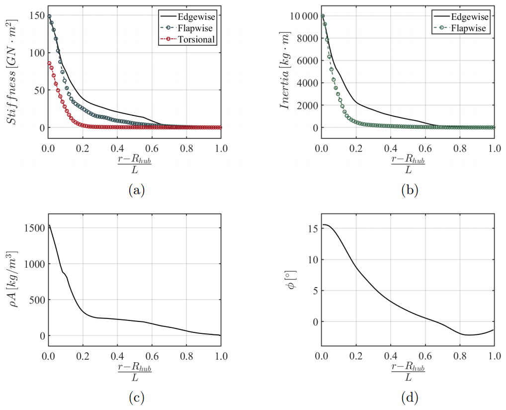
Figure B1Structural properties of the blade along the span: (a) stiffness, (b) inertia, (c) density, (d) local twist angle.
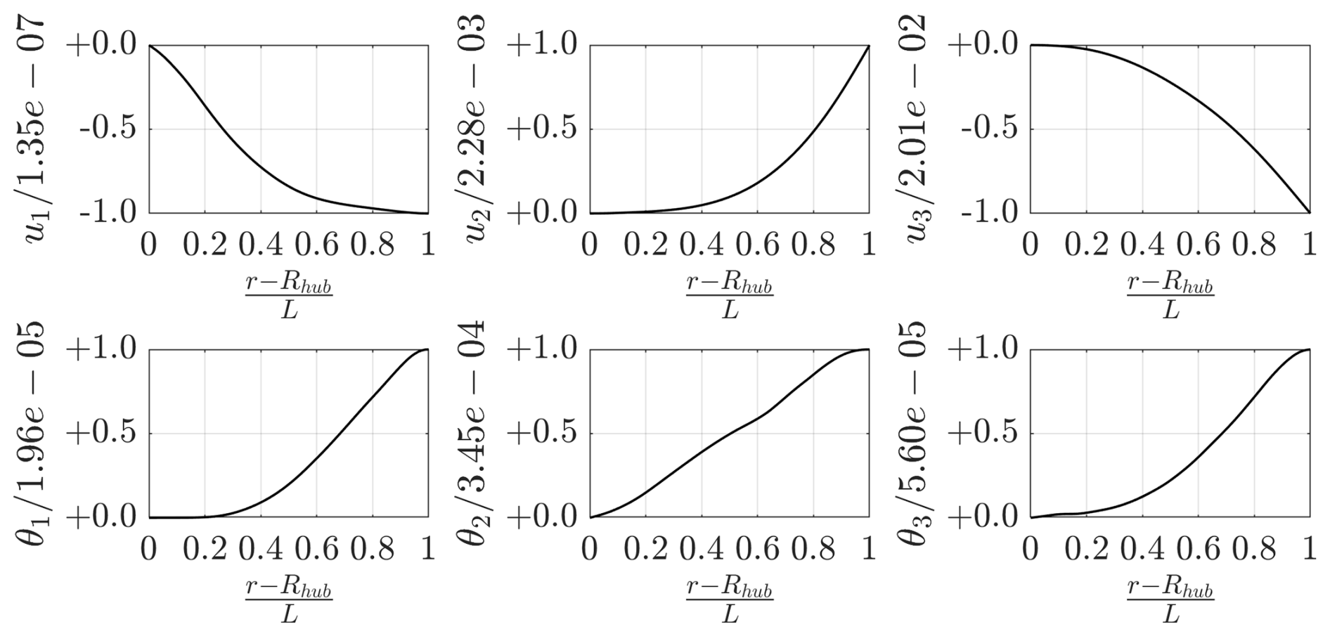
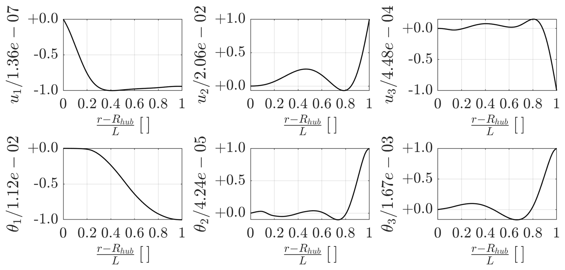
The CFD software used in this study is an in-house research code developed and continuously maintained by the authors' research group. The code represents the result of several years of internal methodological development and incorporates proprietary implementations that are not publicly available. For this reason, the source code cannot be released through a public repository or distributed to third parties. The numerical methods and computational procedures relevant to this work are described in sufficient detail within the manuscript to ensure the reproducibility of the presented results. Additional information regarding the implementation can be provided by the corresponding author upon reasonable request, provided that such requests do not require the disclosure of proprietary source code. No third-party software code was used to perform the CFD simulations presented in this study beyond standard external libraries required for compilation and execution.
The research data supporting the findings of this study consist primarily of numerical simulation outputs generated using the authors' in-house CFD code. Owing to the large volume of the generated data and their strong dependence on the proprietary software used to produce them, the complete data sets have not been deposited in a public repository. All data necessary to support the conclusions of the study are presented in the manuscript through figures, tables, and quantitative results. Additional simulation data underlying the published results are available from the corresponding author upon reasonable request, provided that the request is scientifically justified and does not involve the disclosure of proprietary software or confidential research materials. No third-party data sets were used in this work.
CB: investigation, writing (original draft), formal analysis, methodology, software, validation. SC: conceptualization, investigation, writing (review and editing), supervision. FM: methodology, software, validation. GDP: formal analysis, writing (review and editing), methodology, software. SL: conceptualization, software, supervision. PDP: conceptualization, investigation, writing (review and editing), supervision.
The contact author has declared that none of the authors has any competing interests.
Publisher's note: Copernicus Publications remains neutral with regard to jurisdictional claims made in the text, published maps, institutional affiliations, or any other geographical representation in this paper. The authors bear the ultimate responsibility for providing appropriate place names. Views expressed in the text are those of the authors and do not necessarily reflect the views of the publisher.
This study has been partially funded under the National Recovery and Resilience Plan (NRRP), Mission 4 Component 2 Investment 1.3 – Call for tender No. 1561 of 11.10.2022 Project code PE0000021, Project title “Network 4 Energy Sustainable Transition – NEST”, and under the PRIN grant no. 20229YJP33, “Diffuser augmented Wind Turbines for URBban environments” (DWTURB). Both are grants of Ministero dell’Università e della Ricerca (MUR), funded by the European Union – NextGenerationEU. The cooperative work on the 15 MW NREL wind turbine within the IEA WIND TASK 47 – TURBINIA is also acknowledged. We acknowledge ISCRA for awarding this project access to the LEONARDO supercomputer, owned by the EuroHPC Joint Undertaking, hosted by CINECA (Italy).
This study has been partially funded by the Ministero dell'Università e della Ricerca (project code PE0000021; grant no. 20229YJP33), funded by the European Union “NextGenerationEU”. ISCRA has awarded this project access to the LEONARDO supercomputer, owned by the EuroHPC Joint Undertaking, hosted by CINECA (Italy) (grant nos. IsCc6_WINDAERO and IsCd4_WINSEAv).
This paper was edited by Emmanuel Branlard and reviewed by two anonymous referees.
Abdel Hafeez, M. M. and El-Badawy, A. A.: Flutter limit investigation for a horizontal axis wind turbine blade, J. Vib. Acoust., 140, 041014, https://doi.org/10.1115/1.4039402, 2018. a
Allah, V. A. and Sha ei Mayam, M. H.: Large Eddy Simulation of flow around a single and two in-line horizontal-axis wind turbines, Energy, 121, 533–544, 2017. a, b
Bartl, J. and Sætran, L.: Blind test comparison of the performance and wake flow between two in-line wind turbines exposed to different turbulent inflow conditions, Wind Energ. Sci., 2, 55–76, https://doi.org/10.5194/wes-2-55-2017, 2017. a
Bayati, I., Belloli, M., Bernini, L., and Zasso, A.: Aerodynamic design methodology for wind tunnel tests of wind turbine rotors, J. Wind Eng. Ind. Aerod., 167, 217–227, https://doi.org/10.1016/j.jweia.2017.05.004, 2017. a
Bazilevs, Y., Hsu, M.-C., Kiendl, J., Wüchner, R., and Bletzinger, K.-U.: 3D simulation of wind turbine rotors at full scale. Part II: Fluid-structure interaction modeling with composite blades, Int. J. Numer. Meth. Fl., 65, 236–253, https://doi.org/10.1002/fld.2454, 2011. a
Bernardi, C., Posta, G. D., Palma, P. D., Leonardi, S., Bernardoni, F., Bernardini, M., and Cherubini, S.: The effect of the tower's modeling on the aero-elastic response of the NREL 5 MW wind turbine, J. Phys. Conf. Ser., 2505, 012037, https://doi.org/10.1088/1742-6596/2505/1/012037, 2023. a, b, c, d, e, f, g, h
Boorsma, K., Greco, L., and Bedon, G.: Rotor wake engineering models for aeroelastic applications, J. Phys. Conf. Ser., 1037, 062013, https://doi.org/10.1088/1742-6596/1037/6/062013, 2018. a
Boorsma, K., Schepers, G., Aagard Madsen, H., Pirrung, G., Sørensen, N., Bangga, G., Imiela, M., Grinderslev, C., Meyer Forsting, A., Shen, W. Z., Croce, A., Cacciola, S., Schaffarczyk, A. P., Lobo, B., Blondel, F., Gilbert, P., Boisard, R., Höning, L., Greco, L., Testa, C., Branlard, E., Jonkman, J., and Vijayakumar, G.: Progress in the validation of rotor aerodynamic codes using field data, Wind Energ. Sci., 8, 211–230, https://doi.org/10.5194/wes-8-211-2023, 2023. a
Boorsma, K., Schepers, J. G., Pirrung, G. R., Madsen, H. A., Sørensen, N. N., Grinderslev, C., Bangga, G., Imiela, M., Croce, A., Cacciola, S., Blondel, F., Branlard, E., and Jonkman, J.: Challenges in Rotor Aerodynamic Modeling for Non-Uniform Inflow Conditions, J. Phys. Conf. Ser., 2767, 022006, https://doi.org/10.1088/1742-6596/2767/2/022006, 2024. a
Burton, T., Jenkins, N., Sharpe, D., and Bossanyi, E.: Wind energy handbook, John Wiley & Sons, ISBN 978-0-470-69975-1, 2011. a
Cacciola, S., Croce, A., Bangga, G., Pirrung, G., Bonfils, N., Greco, L., Aryan, N., Castorrini, A., Morici, V., Chetan, M., Jonkman, J., Branlard, E., Cherubini, S., Bernardi, C., Boorsma, K., Schepers, J. G., Savenije, F. J., Bianchini, A., Pagamonci, L., Papi, F., Hach, O., Imiela, M., and Witt, D.: A Comparative Study of Different Modeling Tools and Analysis Techniques for Aeroelastic Stability Assessment. in Proceedings of The Science of Making Torque from Wind (TORQUE 2026): Aerodynamics, aeroelasticity, and aeroacoustics, 042028, IOP Publishing, Journal of Physics: Conference Series, no. 4, vol. 3224, 2026 The Science of making Torque from wind, Bruges, Belgium, 03/06/2026, https://doi.org/10.1088/1742-6596/3224/4/042028, 2026. a, b, c
Chen, X.: Experimental investigation on structural collapse of a large composite wind turbine blade under combined bending and torsion, Compos. Struct., 160, 435–445, https://doi.org/10.1016/j.compstruct.2016.10.086, 2017. a
Chung, J. and Hulbert, G. M.: A Time Integration Algorithm for Structural Dynamics With Improved Numerical Dissipation: The Generalized-α Method, J. Appl. Mech., 60, 371–375, https://doi.org/10.1115/1.2900803, 1993. a
Ciri, U., Petrolo, G., Salvetti, M. V., and Leonardi, S.: Large-Eddy Simulations of Two In-Line Turbines in a Wind Tunnel with Different Inflow Conditions, Energies, 10, 821, https://doi.org/10.3390/en10060821, 2017. a, b
Courant, R., Friedrichs, K., and Lewy, H.: On the partial difference equations of mathematical physics, IBM J. Res. Dev., 11, 215–234, https://doi.org/10.1147/rd.112.0215, 1967. a
Damgaard, M., Ibsen, L. B., Andersen, L. V., and Andersen, J. K.: Cross-wind modal properties of offshore wind turbines identified by full scale testing, J. Wind Eng. Ind. Aerod., 116, 94–108, https://doi.org/10.1016/j.jweia.2013.03.003, 2013. a
Damiani, R., Jonkman, J., and Hayman, G.: SubDyn user's guide and theory manual, Tech. rep., National Renewable Energy Lab.(NREL), Golden, CO, USA, 2015. a
Della Posta, G., Leonardi, S., and Bernardini, M.: A two-way coupling method for the study of aeroelastic effects in large wind turbines, Renewable Energy, 190, 971–992, https://doi.org/10.1016/j.renene.2022.03.158, 2022. a, b, c, d, e
Della Posta, G., Leonardi, S., and Bernardini, M.: Large eddy simulations of a utility-scale horizontal axis wind turbine including unsteady aerodynamics and fluid-structure interaction modelling, Wind Energy, 26, 98–125, https://doi.org/10.1002/we.2789, 2023. a, b, c
Dong, X., Lian, J., Wang, H., Yu, T., and Zhao, Y.: Structural vibration monitoring and operational modal analysis of offshore wind turbine structure, Ocean Eng., 150, 280–297, https://doi.org/10.1016/j.oceaneng.2017.12.052, 2018. a
Gaertner, E., Rinker, J., Sethuraman, L., Zahle, F., Anderson, B., Barter, G., Abbas, N., Meng, F., Bortolotti, P., Skrzypinski, W., Scott, G., Feil, R., Bredmose, H., Dykes, K., Sheilds, M., Allen, C., and Viselli, A.: Definition of the IEA 15-Megawatt Offshore Reference Wind Turbine, Tech. rep., International Energy Agency, https://www.nrel.gov/docs/fy20osti/75698.pdf (last access: 10 October 2024), 2020a. a
Gaertner, E., Rinker, J., Sethuraman, L., Zahle, F., Anderson, B., Barter, G., Abbas, N., Meng, F., Bortolotti, P., Skrzypinski, W., Scott, G., Feil, R., Bredmose, H., Dykes, K., Shields, M., Allen, C., and Viselli, A.: Definition of the IEA 15-megawatt offshore reference wind turbine, https://backend.orbit.dtu.dk/ws/portalfiles/portal/238027930/75698.pdf (last access: 10 October 2024), 2020b. a, b, c
Hansen, M.: Aerodynamics of wind turbines, Routledge, ISBN 978-1-138-77507-7, 2015. a
Hansen, M. H.: Aeroelastic instability problems for wind turbines, Wind Energy, 10, 551–577, https://doi.org/10.1002/we.242, 2007. a
Heinz, J.: Partitioned Fluid-Structure Interaction for Full Rotor Computations Using CFD, PhD thesis, DTU Wind Energy, Denmark, ISBN 978-87-92896-74-2, 2013. a
Jonkman, J.: The New Modularization Framework for the FAST Wind Turbine CAE Tool, in: 51st AIAA Aerospace Sciences Meeting including the New Horizons Forum and Aerospace Exposition, Grapevine (Dallas/Ft. Worth Region), Texas, 7–10 January 2013, AIAA 2013-202, https://doi.org/10.2514/6.2013-202, 2013. a
Jonkman, J. M., Hayman, G., Jonkman, B., Damiani, R., and Murray, R.: AeroDyn v15 user’s guide and theory manual, NREL Draft Report, Vol. 46, 2015. a
Krogstad, P.-A., Satran, L., and Adaramola, M. S.: Blind Test 3: calculations of the performance and wake development behind two in-line and offset model wind turbines, J. Fluid. Struct., 52, 65–80, 2015. a, b
Manwell, J. F., McGowan, J. G., and Rogers, A. L.: Wind energy explained: theory, design and application, John Wiley & Sons, ISBN 978-0-470-01500-1, 2010. a
Martinez-Tossas, L. A., Churchfield, M. J., Yilmaz, A. E., Sarlak, H., Johnson, P. L., Sørensen, J. N., Meyers, J., and Meneveau, C.: Comparison of four large-eddy simulation research codes and effects of model coefficient and inflow turbulence in actuator-line-based wind turbine modeling, J. Renew. Sustain. Ener., 10, https://doi.org/10.1063/1.5004710, 2018. a
Moeller, T.: Blade cracks signal new stress problem, WindPower Monthly, Vol. 25, 1997. a
Moriarty, P. J. and Hansen, A. C.: AeroDyn Theory Manual, National Renewable Energy Laboratory, https://doi.org/10.2172/15014831, 2005. a
Orlandi, P.: Fluid flow phenomena: a numerical toolkit, Vol. 55, Springer Science & Business Media, https://doi.org/10.1007/978-94-011-4281-6, 2012. a
Orlandi, P. and Leonardi, S.: DNS of turbulent channel flows with two-and three-dimensional roughness, J. Turbul., 7, N73, https://doi.org/10.1080/14685240600827526, 2006. a
Pagamonci, L., Papi, F., Balduzzi, F., Xie, S., Sadique, J., Scienza, P., and Bianchini, A.: To what extent is aeroelasticity impacting multi-megawatt wind turbine upscaling? A critical assessment, J. Phys. Conf. Ser., 2648, 012005, https://doi.org/10.1088/1742-6596/2648/1/012005, 2023. a, b, c, d
Pino Martín, M., Piomelli, U., and Candler, G. V.: Subgrid-scale models for compressible large-eddy simulations, Theor. Comp. Fluid Dyn., 13, 361–376, 2000. a
Porte-Agel, F. and Wu, Y.-T.: Large-Eddy Simulation of Wind-Turbine Wakes: Evaluation of Turbine Parametrisations, Bound.-Lay. Meteorol., 138, 345–366, 2011. a
Reschke, C.: Flight loads analysis with inertially coupled equations of motion, in: AIAA Atmospheric Flight Mechanics Conference and Exhibit, San Francisco, California, 15–18 August 2005, AIAA 2005-6026, https://doi.org/10.2514/6.2005-6026, 2005. a
Ribeiro, A. F. P., Casalino, D., and Ferreira, C. S.: Nonlinear inviscid aerodynamics of a wind turbine rotor in surge, sway, and yaw motions using a free-wake panel method, Wind Energ. Sci., 8, 661–675, https://doi.org/10.5194/wes-8-661-2023, 2023. a
Rinker, J., Gaertner, E., Zahle, F., Skrzypiński, W., Abbas, N., Bredmose, H., Barter, G., and Dykes, K.: Comparison of loads from HAWC2 and OpenFAST for the IEA Wind 15 MW Reference Wind Turbine, J. Phys. Conf. Ser., 1618, 052052, https://doi.org/10.1088/1742-6596/1618/5/052052, 2020. a
Sabale, A. K. and Gopal, N. K. V.: Nonlinear Aeroelastic Analysis of Large Wind Turbines Under Turbulent Wind Conditions, AIAA Journal, 57, 4416–4432, https://doi.org/10.2514/1.J057404, 2019. a
Saltari, F., Riso, C., Matteis, G. D., and Mastroddi, F.: Finite-element-based modeling for flight dynamics and aeroelasticity of flexible aircraft, J. Aircraft, 54, 2350–2366, https://doi.org/10.2514/1.C034159, 2017. a
Santoni, C., Ciri, U., Rotea, M., and Leonardi, S.: Development of a high fidelity CFD code for wind farm control, in: 2015 American Control Conference (ACC), Chicago, IL, USA, 1–3 July 2015, IEEE, 1715–1720, https://doi.org/10.1109/ACC.2015.7170980, 2015. a
Santoni, C., Carrasquillo, K., Arenas-Navarro, I., and Leonardi, S.: Effect of tower and nacelle on the flow past a wind turbine, Wind Energy, 20, 1927–1939, https://doi.org/10.1002/we.2130, 2017. a, b, c, d, e, f, g, h
Santoni, C., García-Cartagena, E. J., Ciri, U., Zhan, L., Valerio Iungo, G., and Leonardi, S.: One-way mesoscale-microscale coupling for simulating a wind farm in North Texas: Assessment against SCADA and LiDAR data, Wind Energy, 23, 691–710, https://doi.org/10.1002/we.2452, 2020. a
Schepers, J., Boorsma, K., Madsen, H., Pirrung, G., Bangga, G., Guma, G., Lutz, T., Potentier, T., Braud, C., Guilmineau, E., Croce, A., Cacciola, S., Schaffarczyk, A. P., Lobo, B. A., Ivanell, S., Asmuth, H., Bertagnolio, F., Sørensen, N., Shen, W. Z., Grinderslev, C., Forsting, A. M., Blondel, F., Bozonnet, P., Boisard, R., Yassin, K., Hoening, L., Stoevesandt, B., Imiela, M., Greco, L., Testa, C., Magionesi, F., Vijayakumar, G., Ananthan, S., Sprague, M. A., Branlard, E., Jonkman, J., Carrion, M., Parkinson, S., and Cicirello, E.: IEA Wind TCP Task 29, Phase IV: Detailed Aerodynamics of Wind Turbines, Zenodo, https://doi.org/10.5281/zenodo.4813068, 2021. a, b
Schepers, J. G., Boorsma, K., Bois, R., Bangga, G., Jonkman, J., Kelley, C., Branlard, E., Gonçalves Pinto, W., Imiela, M., Hach, O., Greco, L., Testa, C., Aryan, N., Madsen, H., Croce, A., Cacciola, S., Pirrung, G., Sørensen, N., Grinderslev, C., Bernardi, C., Cherubini, S., Bianchini, A., Papi, F., Pagamonci, L., Braud, C., Höning, L., Theron, J., and Mohan, K.: Turbinia, turbulent inflow innovative aerodynamics, Tech. rep., IEA Wind TCP – Task47, Zenodo, https://doi.org/10.5281/zenodo.17897185, 2025. a, b, c, d
Shen, W. Z., Mikkelsen, R., Sørensen, J. N., and Bak, C.: Tip loss corrections for wind turbine computations, Wind Energy, 8, 457–475, https://doi.org/10.1002/we.153, 2005. a, b
Sorensen, J. and Shen, W. Z.: Numerical Modeling of Wind Turbine Wakes, Journal of Fluids Engineering, 124, 393–399, https://doi.org/10.1115/1.1471361, 2002. a
Sørensen, J. N.: Aerodynamic aspects of wind energy conversion, Annu. Rev. Fluid Mech., 43, 427–448, https://doi.org/10.1146/annurev-fluid-122109-160801, 2011. a
Stevens, R. J., Martinez-Tossas, L. A., and Meneveau, C.: Comparison of wind farm large eddy simulations using actuator disk and actuator line models with wind tunnel experiments, Renewable Energy, 116, 470–478, 2018. a
Trigaux, F., Chatelain, P., and Winckelmans, G.: Investigation of blade flexibility effects on the loads and wake of a 15 MW wind turbine using a flexible actuator line method, Wind Energ. Sci., 9, 1765–1789, https://doi.org/10.5194/wes-9-1765-2024, 2024. a, b, c, d, e
Troldborg, N.: Actuator line modeling of wind turbine wakes, PhD thesis, Technical University of Denmark, ISBN 978-87-89502-80-9, 2009. a
Vermeer, L., Sørensen, J. N., and Crespo, A.: Wind turbine wake aerodynamics, Prog. Aerosp. Sci., 39, 467–510, https://doi.org/10.1016/S0376-0421(03)00078-2, 2003. a
Wang, L., Liu, X., and Kolios, A.: State of the art in the aeroelasticity of wind turbine blades: Aeroelastic modelling, Renewable and Sustainable Energy Reviews, 64, 195–210, https://doi.org/10.1016/j.rser.2016.06.007, 2016a. a
Wang, Q., Jonkman, J., Sprague, M., and Jonkman, B.: Beamdyn user's guide and theory manual, National Renewable Energy Laboratory, 2016b. a, b, c
Yu, D. O. and Kwon, O. J.: Predicting wind turbine blade loads and aeroelastic response using a coupled CFD-CSD method, Renewable Energy, 70, 184–196, https://doi.org/10.1016/j.renene.2014.03.033, 2014. a
Zahle, F., Barlas, A., Lønbæk, K., Bortolotti, P., Zalkind, D., Wang, L., Labuschagne, C., Sethuraman, L., and Barter, G.: Definition of the IEA Wind 22-Megawatt Offshore Reference Wind Turbine, Technical University of Denmark (DTU), 68 pp., https://doi.org/10.11581/DTU.00000317, 2024. a
Zhang, Y., Song, Y., Shen, C., and Chen, N.-Z.: Aerodynamic and structural analysis for blades of a 15MW floating offshore wind turbine, Ocean Eng., 287, 115785, https://doi.org/10.1016/j.oceaneng.2023.115785, 2023. a
Zheng, J., Wang, N., Wan, D., and Strijhak, S.: Numerical investigations of coupled aeroelastic performance of wind turbines by elastic actuator line model, Appl. Energ., 330, 120361, https://doi.org/10.1016/j.apenergy.2022.120361, 2023. a
- Abstract
- Introduction
- Methodologies
- Flow and structural setup
- Results and discussion
- Conclusions
- Appendix A: Grid convergence study for LES
- Appendix B: Validation of the structural model
- Code availability
- Data availability
- Author contributions
- Competing interests
- Disclaimer
- Acknowledgements
- Financial support
- Review statement
- References
- Abstract
- Introduction
- Methodologies
- Flow and structural setup
- Results and discussion
- Conclusions
- Appendix A: Grid convergence study for LES
- Appendix B: Validation of the structural model
- Code availability
- Data availability
- Author contributions
- Competing interests
- Disclaimer
- Acknowledgements
- Financial support
- Review statement
- References