A North Sea in situ evaluation of the Fitch wind farm parameterization within the Mellor–Yamada–Nakanishi–Niino and 3D planetary boundary layer schemes

Wind resource assessments and wind power forecasts that account for wind farm wakes are sensitive to the choice of planetary boundary layer (PBL) scheme. This work compares the one-dimensional Mellor–Yamada–Nakanishi–Niino (MYNN) PBL scheme with a three-dimensional PBL (3DPBL) scheme, evaluating predictions made with both schemes against two sets of North Sea in situ observations of wind farm wakes. The optimal PBL scheme varies based on the observations (FINO1 tower vs. aircraft), the quantity of interest (wind speed vs. turbulence kinetic energy [TKE]), and the error metric (bias, centered root mean square error [cRMSE], R², and earth mover’s distance [EMD]). Whereas 3DPBL wind speeds outperform MYNN wind speeds with respect to the cRMSE at the FINO1 site located at a single point within the turbine rotor layer, 3DPBL TKE bias is larger than MYNN TKE bias when compared to aircraft observations taken 100 m above a wind farm. Wind speeds in the aircraft region are ambiguous with regard to which PBL scheme is optimal. Aircraft MYNN wind speeds outperform 3DPBL wind speeds with respect to R² and cRMSE but underperform with respect to bias and EMD. Future evaluations across broader temporal and spatial scales may offer further insight into model differences.

1 Introduction

More energy generation technologies are being developed and deployed as global energy demand continues to increase. This new energy generation is also becoming increasingly renewable. Offshore wind is one renewable technology that continues to grow, especially in the North Sea and Baltic areas (Backwell et al., 2024). Wind and wake forecasts are becoming increasingly crucial in project planning. These forecasts are sensitive to the underlying wind resource (Optis and Perr-Sauer, 2019), and meteorological wind turbine wake models are continually in development (Fischereit et al., 2022a).

Wind turbine impacts on the weather are often expressed through wind farm parameterizations (WFPs) (Fischereit et al., 2022a) within numerical weather prediction (NWP) models like the Weather Research and Forecasting (WRF) model (Skamarock et al., 2021). Most WFPs treat wind farms as elevated sources of turbulence and sinks of momentum (Baidya Roy et al., 2004; Fitch et al., 2012; Adams and Keith, 2013), especially after the importance of treating the wind farm as an elevated source of drag (rather than as being proximate to the surface) was demonstrated (Fitch et al., 2013). WFPs may include (Fitch et al., 2012) or exclude (Volker et al., 2015) an explicit source of turbulence kinetic energy (TKE), and this decision drives differences in both wind speeds and TKE (Shepherd et al., 2020; Pryor et al., 2020; Larsén and Fischereit, 2021; García-Santiago et al., 2024; Quint et al., 2025). WFPs also differ based on if and how they represent subgrid-scale processes (Abkar and Porté-Agel, 2015; Volker et al., 2015; Pan and Archer, 2018; Ma et al., 2022), which is important when multiple turbines need to be represented within one grid cell.

Wind fields predicted from NWP simulations are also sensitive to modeling choices within the WFP. Simulated wind fields depend on horizontal and vertical grid cell spacing (Lee and Lundquist, 2017; Mangara et al., 2019; Tomaszewski and Lundquist, 2020; Pryor et al., 2020), the strength of the explicit TKE source (Fitch et al., 2012; Vanderwende et al., 2016; Rajewski et al., 2016; Mangara et al., 2019; Tomaszewski and Lundquist, 2020; Siedersleben et al., 2020), the advection option (Siedersleben et al., 2020; Archer et al., 2020; Larsén and Fischereit, 2021), and the planetary boundary layer (PBL) scheme choice (Peña et al., 2023). Within the PBL scheme, parameterizations of physical quantities can further affect results. For example, the turbulence dissipation rate, ϵ, affects modeled wind fields within the Mellor–Yamada–Nakanishi–Niino (MYNN) scheme (Yang et al., 2017; Bodini et al., 2020).

Given that WFPs are impacted by multiple uncertainties and that these uncertainties have significant implications for power predictions, recent efforts have focused on WFP intercomparison and validation. Winds from WFP simulations have been validated against meteorological tower observations, aircraft observations, synthetic aperture radar (SAR), and lidar measurements (Fischereit et al., 2022a). However, WFP intercomparison and validation efforts have experienced challenges. Observations are generally staged at a distance from the wind farms that allows for validation of only the background meteorology as opposed to the wake behavior. Conclusions drawn from these validation studies may also be influenced by site-specific or meteorological conditions. Further, many previous WRF intercomparison studies contained a TKE advection bug in the Fitch et al. (2012) scheme, as identified in Archer et al. (2020).

A recent North Sea measurement campaign has stimulated interest in WFP intercomparison and validation efforts. The Wind Park Far Field (WIPAFF) project was an aircraft expedition to understand offshore wind wake behavior in the German Bight. This expedition took place in a location with multiple wind farms, with 41 total flights between 6 September 2016 and 15 October 2017 (Platis et al., 2018; Bärfuss et al., 2021). Siedersleben et al. (2018b) modeled a case study that included 1 d of these aircraft observations and found that, because of challenges in characterizing air–sea interactions with a mesoscale model, improving background flow characterization contributed greater model improvement than any wind-farm-specific parameter configuration. Siedersleben et al. (2018a) then extended the analysis of this one case study to demonstrate the presence of hub height potential temperature and water vapor wakes during stably stratified conditions. Siedersleben et al. (2020) then leveraged 3 d of these aircraft observations that occurred under stable conditions to explore the sensitivity of grid cell spacing and TKE advection within the Fitch parameterization. Larsén and Fischereit (2021) extended the work of Siedersleben et al. (2020) by comparing the explicit wake parameterization (EWP) (Volker et al., 2015) and Fitch (Fitch et al., 2012) schemes and exploring model performance during wind farm interactions with low-level jets (LLJs), and this work was then extended to introduce wave coupling (Larsén et al., 2024). Ali et al. (2023) also used data from 1 d of the Siedersleben et al. (2020) case study to validate five (Fitch et al., 2012; Volker et al., 2015; Abkar and Porté-Agel, 2015; Pan and Archer, 2018; Redfern et al., 2019) common WFPs with aircraft measurements, as well as nearby meteorological tower and synthetic aperture radar observations.

The influence of the PBL scheme choice is one parameter that has not yet been considered for this case study and that has generally been absent in the literature evaluating WFPs (Fischereit et al., 2022a). Although the influence of the PBL scheme on the wind resource has been an active field of research in turbine-free NWP simulations (Zhang and Zheng, 2004; Jankov et al., 2005; Li and Pu, 2008; Nolan et al., 2009; Shin and Hong, 2011; Draxl et al., 2014), research regarding the impacts of the PBL scheme on turbine simulations has been limited because the default Fitch WFP has, until recently, been integrated with only the MYNN PBL scheme (Nakanishi and Niino, 2009).

However, the recent development (Kosović et al., 2020; Juliano et al., 2022; Eghdami et al., 2022) and evaluation (Arthur et al., 2022; Peña et al., 2023; Arthur et al., 2025) of the US National Science Foundation National Center for Atmospheric Research (NCAR) three-dimensional PBL (3DPBL) scheme, followed by its integration with the Fitch scheme (Rybchuk et al., 2022), offers an opportunity to better understand the sensitivity of wind farm behavior to PBL scheme choice. The 3DPBL scheme is based on the Mellor and Yamada (1982) scheme and accounts for the 3D effects of turbulence by explicitly calculating the horizontal momentum, heat, and moisture flux divergences. Similarly to the MYNN PBL scheme, the 3DPBL scheme is a level-2.5 model, such that TKE is a prognostic variable. The 3DPBL scheme reduces errors in potential temperature, wind speed, and TKE relative to the one-dimensional (1D) MYNN scheme when compared to cold-air-pool observations in the Columbia River basin (Arthur et al., 2022). The potential value of the 3DPBL scheme compared to that of the 1D MYNN scheme may also depend on the grid cell resolution (Peña et al., 2023).

This work compares the MYNN PBL scheme with a 3DPBL scheme by validating against both tower and aircraft observations for a North Sea case study. These results address the research gap regarding the sensitivity of wake behavior to the PBL scheme and offer guidance to the offshore forecasting community. This paper is organized as follows. In Sect. 2, we describe the North Sea case study, detail the observational datasets, and outline the WRF simulation setup. In Sect. 3, we present the results from our WRF simulations and compare these results to meteorological tower and aircraft observations associated with the case study. In Sect. 4, we offer potential implications of the differing performance between the PBL schemes for wind resource assessments and wind power forecasting.

2 Methods

2.1 PBL scheme comparison

The analysis in this work compares the MYNN 2.5 (Mellor and Yamada, 1982; Olson et al., 2019) and NCAR 3DPBL (Juliano et al., 2022) schemes. A brief description of the differences between these two schemes is provided here, while a more complete description of the differences between the 3DPBL and MYNN schemes can be found in Kosović et al. (2020), Juliano et al. (2022), and Rybchuk et al. (2022). Note that the 3DPBL scheme described in this work is not to be confused with 3DTKE (Zhang et al., 2018); 3DTKE is a scale-adaptive model that relies on a level-3 closure. More information about 3DTKE can be found in Zhang et al. (2018).

2.1.1 Governing equations

The MYNN and 3DPBL schemes share a common origin with the Mellor and Yamada (1982) governing equations:

$$\begin{array}{}\text{(1)}& {\displaystyle \frac{\partial U_i}{\partial t}}+U_j{\displaystyle \frac{\partial U_i}{\partial x_j}}=-{\mathit{ϵ}}_{ijk}{f}_j{U}_k-{\displaystyle \frac{\mathrm{1}}{\mathit{\rho }}}{\displaystyle \frac{\partial P}{\partial x_i}}-{\displaystyle \frac{\partial <u_j{u}_i>}{\partial x_j}}-g_i,\text{(2)}& {\displaystyle \frac{\partial \mathrm{\Theta }}{\partial t}}+U_j{\displaystyle \frac{\partial \mathrm{\Theta }}{\partial x_j}}=-{\displaystyle \frac{\partial <u_j\mathrm{\Theta }>}{\partial x_j}},\end{array}$$

where the ensemble mean momentum per unit mass is U_i, potential temperature is θ, P describes the mean kinematic pressure, g_i captures the influence of gravity, and f_k is the Coriolis vector.

With a level-2.5 closure, these governing equations become

$$\begin{array}{}\text{(3)}& {\displaystyle \frac{\partial q^{\mathrm{2}}}{\partial t}}+U_k{\displaystyle \frac{\partial q^{\mathrm{2}}}{\partial x_k}}={\displaystyle \frac{\partial }{\partial x_k}}\left[lq{S}_q{\displaystyle \frac{\partial q^{\mathrm{2}}}{\partial x_k}}\right]+\mathrm{2}(P_{\mathrm{s}}+P_{\mathrm{b}}-\mathit{ϵ}),\text{(4)}& {\displaystyle }\begin{array}{rl}<u_i{u}_j>& ={\displaystyle \frac{{\mathit{\delta }}_{ij}}{\mathrm{3}}}{q}^{\mathrm{2}}-\mathrm{3}{\displaystyle \frac{l_{\mathrm{1}}}{q}}\left[\right(<u_k{u}_i>-C_{\mathrm{1}}{q}^{\mathrm{2}}{\mathit{\delta }}_{ki}){\displaystyle \frac{\partial U_j}{\partial x_k}}\\ & +(<u_k{u}_j>-C_{\mathrm{1}}{q}^{\mathrm{2}}{\mathit{\delta }}_{kj}){\displaystyle \frac{\partial U_i}{\partial x_k}}\\ & -{\displaystyle \frac{\mathrm{2}}{\mathrm{3}}}{\mathit{\delta }}_{ij}<u_k{u}_n>{\displaystyle \frac{\partial U_n}{\partial x_k}}]-\mathrm{3}{\displaystyle \frac{l_{\mathrm{1}}}{q}}\mathit{\beta }[g_j<u_i{\mathit{\theta }}_v>\\ & +g_i<u_j{\mathit{\theta }}_v>-{\displaystyle \frac{\mathrm{2}}{\mathrm{3}}}{\mathit{\delta }}_{ij}{g}_n<u_n{\mathit{\theta }}_v>],\end{array}\text{(5)}& {\displaystyle }<{\mathit{\theta }}_v^{\mathrm{2}}>=-{\displaystyle \frac{{\mathrm{\Lambda }}_{\mathrm{2}}}{q}}<u_k{\mathit{\theta }}_v>{\displaystyle \frac{\partial {\mathrm{\Theta }}_v}{\partial x_k}},\text{(6)}& {\displaystyle }\begin{array}{rl}<u_j{\mathit{\theta }}_v>& =-\mathrm{3}{\displaystyle \frac{l_{\mathrm{2}}}{q}}[<u_j{u}_k>{\displaystyle \frac{\partial {\mathrm{\Theta }}_v}{\partial x_k}}+<u_k{\mathit{\theta }}_v>{\displaystyle \frac{\partial U_j}{\partial x_k}}\\ & +\mathit{\beta }{g}_j<{\mathit{\theta }}_v^{\mathrm{2}}>],\end{array}\end{array}$$

such that $q^{\mathrm{2}}=\mathrm{2}\mathrm{TKE}=<u^{\mathrm{2}}>+<v^{\mathrm{2}}>+<w^{\mathrm{2}}>$, where the TKE budget includes shear production $P_{\mathrm{s}}=-<u_i{u}_j>\frac{\partial U_i}{\partial x_k}$, buoyant production $P_{\mathrm{b}}=-\mathit{\beta }{g}_i<u_i{\mathit{\theta }}_v>$, and dissipation $\mathit{ϵ}=\frac{q^{\mathrm{3}}}{{\mathrm{\Lambda }}_{\mathrm{1}}}$. β, S_q, and C₁ are all constants. Finally, the four length scales – l₁, l₂, Λ₁, and Λ₂ – are proportional in such a way that

$$\begin{array}{}\text{(7)}& \left[l_{\mathrm{1}}{\mathrm{\Lambda }}_{\mathrm{1}}{l}_{\mathrm{2}}{\mathrm{\Lambda }}_{\mathrm{2}}\right]=l\left[A_{\mathrm{1}}{B}_{\mathrm{1}}{A}_{\mathrm{2}}{B}_{\mathrm{2}}\right],\end{array}$$

where l represents a master length scale, and A₁, A₂, B₁, and B₂ represent another set of constants.

In this level-2.5 closure, TKE is a prognostic variable, advecting TKE generated within the scheme. This TKE treatment for both MYNN and 3DPBL differs from that for several other PBL schemes (i.e., YSU) and allows for both the MYNN and 3DPBL schemes to integrate with the Fitch WFP (described below) to analyze wind farm wake effects on TKE.

2.1.2 Model differences

From this common origin, the MYNN and 3DPBL schemes differ. First, the two schemes differ in terms of how they represent horizontal turbulent mixing. The MYNN scheme uses Smagorinsky mixing (Smagorinsky, 1963), while the 3DPBL scheme explicitly calculates the horizontal turbulent flux divergences.

A “boundary layer” approximation of the 3DPBL scheme retains the same 3DPBL length scale formulation (and corresponding closure constants) but instead sets the horizontal gradients of the mean quantities and the vertical gradient of the vertical velocity to zero. This 3DPBL approximation is the most commonly used version of the 3DPBL scheme (Rybchuk et al., 2022; Arthur et al., 2022; Sanchez Gomez et al., 2024; Peña et al., 2023; Arthur et al., 2025), and we employ it in this analysis for consistency.

The two PBL schemes also rely on differing master length scales and corresponding closure constants. For this analysis, the 3DPBL scheme uses a Blackadar (1962) master length formulation as follows:

$$\begin{array}{}\text{(8)}& l={\displaystyle \frac{kz}{\mathrm{1}+kz/l_{\mathrm{0}}}},\end{array}$$

such that k is the von Kármán constant, z is the height above ground level, and l₀ is defined by

$$\begin{array}{}\text{(9)}& l_{\mathrm{0}}=\mathit{\alpha }{\displaystyle \frac{\left({\int }_{\mathrm{0}}^{h}qzdz\right)}{\left({\int }_{\mathrm{0}}^{h}qdz\right)}},\end{array}$$

with α as an empirical constant and with the length scale constants determined experimentally under neutrally stratified conditions. These constants are those used in Mellor and Yamada (1982).

The version of MYNN used in this analysis is best characterized by the default (i.e., bl_pbl_opt = 5, bl_mynn_mixlength = 2) configuration of the MYNN-EDMF, as described in Olson et al. (2019). As a result, the closure constants used by the MYNN scheme in this analysis reflect the update in Nakanishi and Niino (2009). The MYNN scheme for this analysis also then calculates its master length scale based on a blending of PBL depth, buoyancy, and surface layer length scales (Olson et al., 2019).

2.1.3 Model locations

The two PBL schemes are also located within different sections of the WRF code base. While the MYNN scheme is located within the physics (/phys/) directory, the 3DPBL scheme resides in the dynamics (/dyn_em/) directory. As a result, the 3DPBL scheme introduces an additional subroutine that ensures both that velocity and those tendencies in the 3DPBL are scaled in the same manner as that for the MYNN scheme and that the Fitch scheme (described in Sect. 2.3) appropriately modifies the 3DPBL TKE tendency. Further details on the implementation of the 3DPBL Fitch integration can be found in Rybchuk et al. (2022).

2.2 North Sea case study

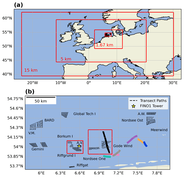
The WIPAFF aircraft expedition explored the impact of several North Sea offshore wind farms (Table 1) on the atmosphere (Platis et al., 2018; Bärfuss et al., 2021) (Fig. 1). The expedition included 41 flights spanning September 2016 to October 2017, where a subset of both transect and profile flights during stably stratified conditions on 14 October 2017 were identified as one common research case study (Siedersleben et al., 2018a, b, 2020; Larsén and Fischereit, 2021; Ali et al., 2023; Larsén et al., 2024).

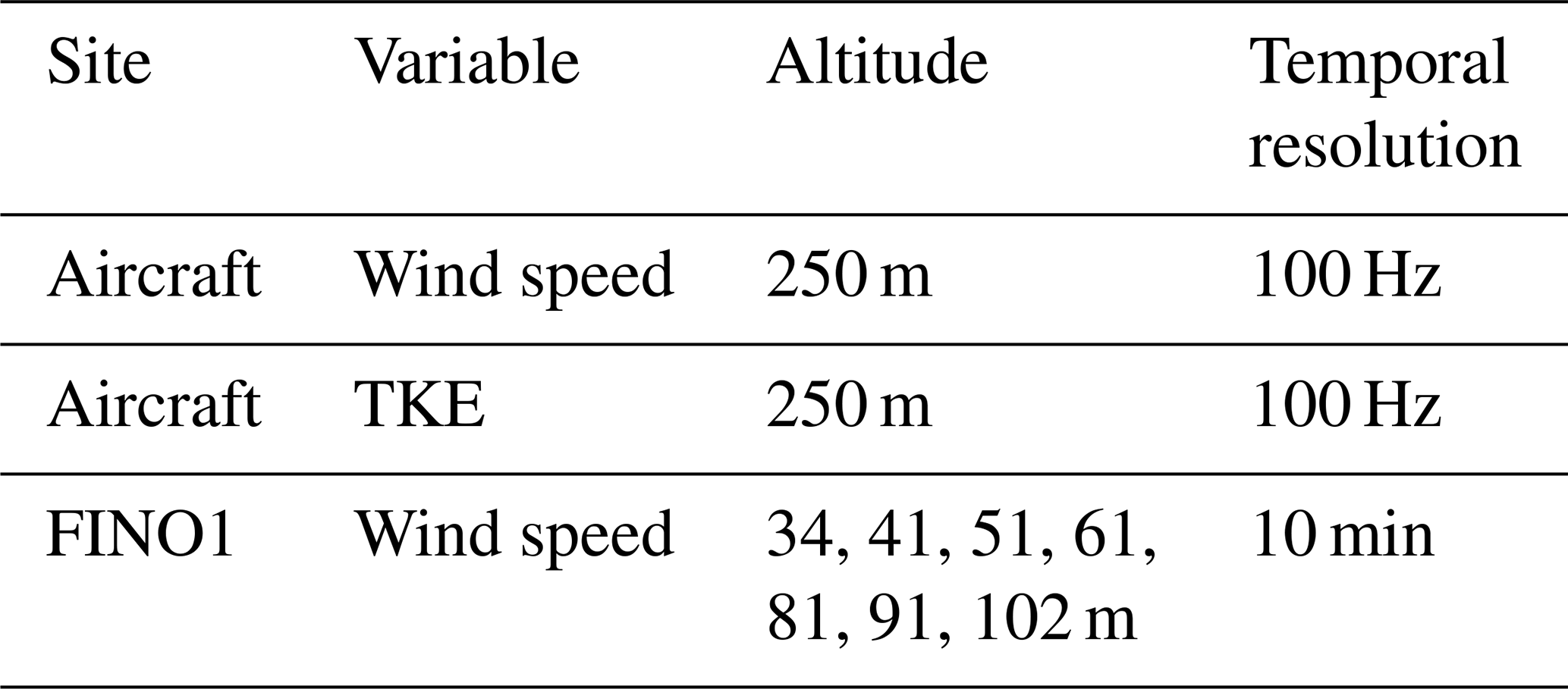
Aircraft measurements from the six transect flights (Table 2) for this 14 October 2017 case study (Platis et al., 2018; Bärfuss et al., 2021) were collected in the vicinity of the Gode wind farm at an altitude of roughly 250 m (Figs. 1b and 2b). The flight paths across the six transects were roughly symmetrical, with transects 1, 3, and 5 traveling towards the northwest and transects 2, 4, and 6 traveling towards the southeast (Platis et al., 2018; Bärfuss et al., 2021). While observations of wind speed, wind direction, temperature, pressure, and relative humidity were collected (Corsmeier et al., 2001), here, we focus on 100 Hz wind speed observations and derived TKE calculations for our evaluation (Table 4).

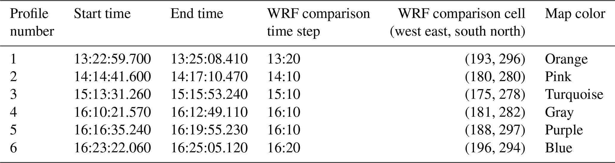
The paths for the six profile flights – described more fully in Platis et al. (2018), Bärfuss et al. (2021), and Larsén and Fischereit (2021) – were taken at the same frequency as that of the transect flights according to the duration outlined in Table 3 and the paths described in Fig. 1b. Because the transect flights occurred at roughly the same altitude and therefore cannot provide profile assessments of atmospheric stability, we employ the temperature, potential temperature, wind speed, wind direction, and TKE observations from these profile flights to assess the atmospheric stability of the region for comparison to the model simulations.

Table 1 Selected wind farm characteristics. Wind turbine performance curves are as in Ali et al. (2023). The wind farms in bold are present in immediate environs of the FINO1 and aircraft measurement regions.

Table 2 Transect timings for 14 October 2017 WIPAFF case.

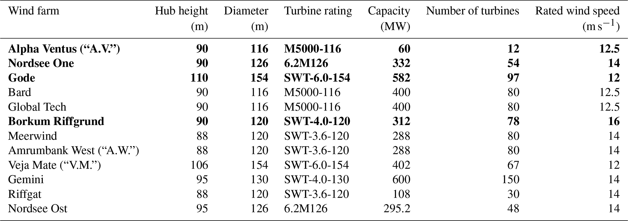
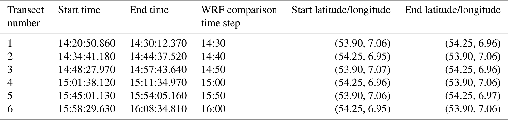
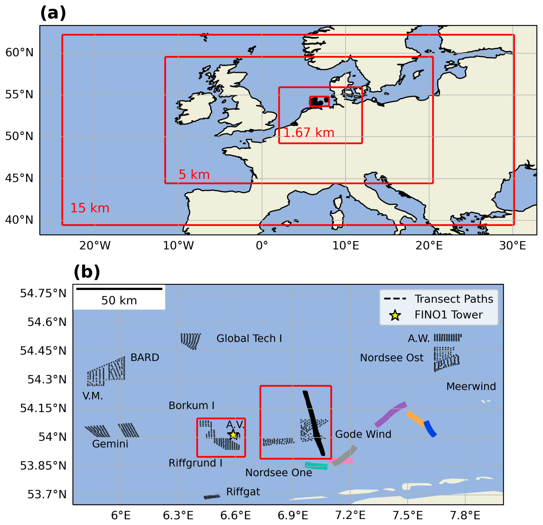
Figure 1 WRF simulation domain for the North Sea 14 October 2017 case study. (a) Three nested domains and a measurement region within the inner domain are outlined in red. (b) Measurement region with wind farms outlined in black, the FINO1 tower marked with a star, and the aircraft transect paths traced in black; the other colored lines indicate the aircraft profile paths outlined in Table 3.

Table 3 Profile timings for 14 October 2017 WIPAFF case used for stability characterization.

This 14 October 2017 North Sea case study also includes observations from a meteorological tower (Figs. 1b and 2a). The FINO1 tower is located immediately west of the Alpha Ventus wind farm and provides observations of wind speed, wind direction, pressure, and temperature averaged over 10 min. This analysis focused on wind speed and included all the available heights: 34, 41, 51, 61, 81, 91, and 102 m. TKE calculations at the FINO1 site were not available due to coarse temporal resolution of the wind observations at the FINO1 site (Table 4).

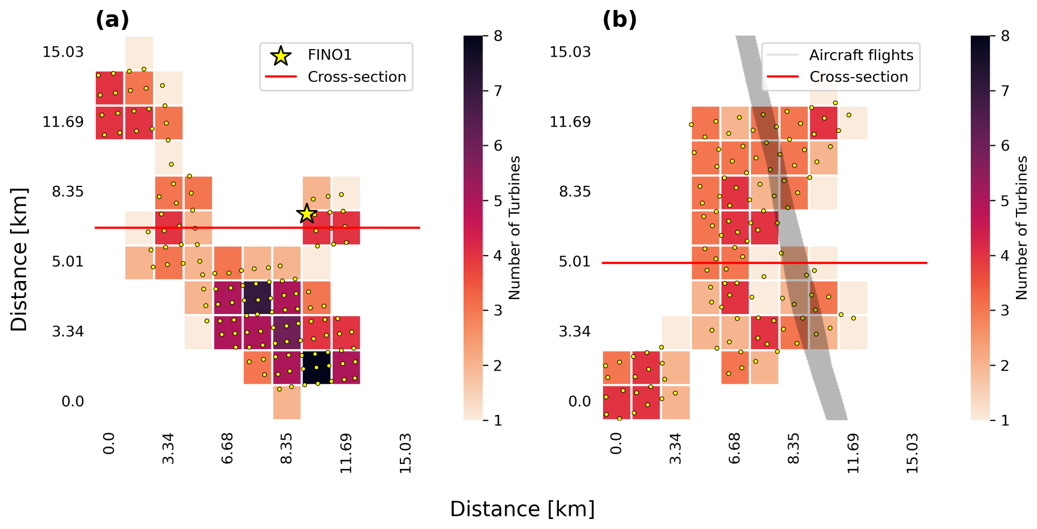
Figure 2 Map of the number of turbines per WRF grid cell in the innermost domain of the 1.67 km resolution for the two regions of interest within the inner region. The two axes represent the WRF grid system. (a) FINO1 site, with the tower marked with a star. (b) Aircraft site, with the six transect paths traced in black.

Table 4 In situ observations for validation.

2.3 Model setup

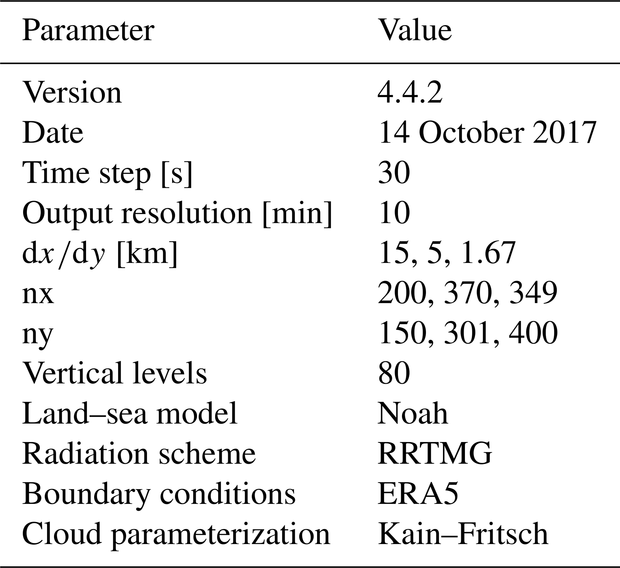
Simulations were performed with the WRF model (Skamarock et al., 2021) with the Fitch WFP (Fitch et al., 2012), modified to incorporate the 3DPBL scheme. Here, the WRF simulations generally followed the setup of Ali et al. (2023) (Table 5). Simulations represented the single day of 14 October 2017 with a 30 s time step in the outer domain and a 10 min output, starting at 00:00:00 UTC with a 12 h spin-up period so that the analysis period starts at 12:00:00 UTC. The region was simulated using three nested domains with an outer horizontal grid size of 15 km and a nesting ratio of 3 so that the innermost domain has a grid size of 1.67 km. Eighty vertical levels were employed, with 17 levels lower than 200 m, and between 8 and 12 levels intersected the turbine's rotor. We used the ERA5 reanalysis (Hersbach et al., 2020) for initial and boundary conditions, and the WRF double-moment six-class microphysics scheme (Hong et al., 2010), the RRTMG shortwave and longwave radiation scheme (Mlawer et al., 1997), the Noah land surface model (Niu et al., 2011), and the Kain–Fritsch cumulus parameterization scheme (Kain, 2004) in the outer domain only.

Table 5 Baseline WRF modeling configuration as an extension of Ali et al. (2023).

Differences also exist between the WRF setup presented in this work and that used in Ali et al. (2023). Here, we varied the PBL scheme to explicitly consider the influence of the PBL scheme on wake behavior for the Fitch WFP. Two PBL schemes were considered: level-2.5 MYNN (“MYNN”) and the NCAR 3DPBL scheme with the PBL approximation (“3DPBL”) as described in Rybchuk et al. (2022). The MYNN scheme is activated in all outer domains for all simulations. Further, Ali et al. (2023) performed their analysis on a modification of WRF v4.5.1, whereas the analysis presented in this work relied on an earlier version of WRF (V4.4.2) in which the 3DPBL scheme is integrated.

Wind farm effects were represented with the Fitch WFP. The wind-speed- and turbine-model-dependent thrust and power coefficients were integrated into the WRF model through turbine specification files (Fig. 3). Individual turbines were also integrated into the WRF grid with a file from Ali et al. (2023) that contains a given turbine's latitude, longitude, and turbine type. We used files from the Ali et al. (2023) repository and extracted the key information to fit the standard Fitch WFP format.

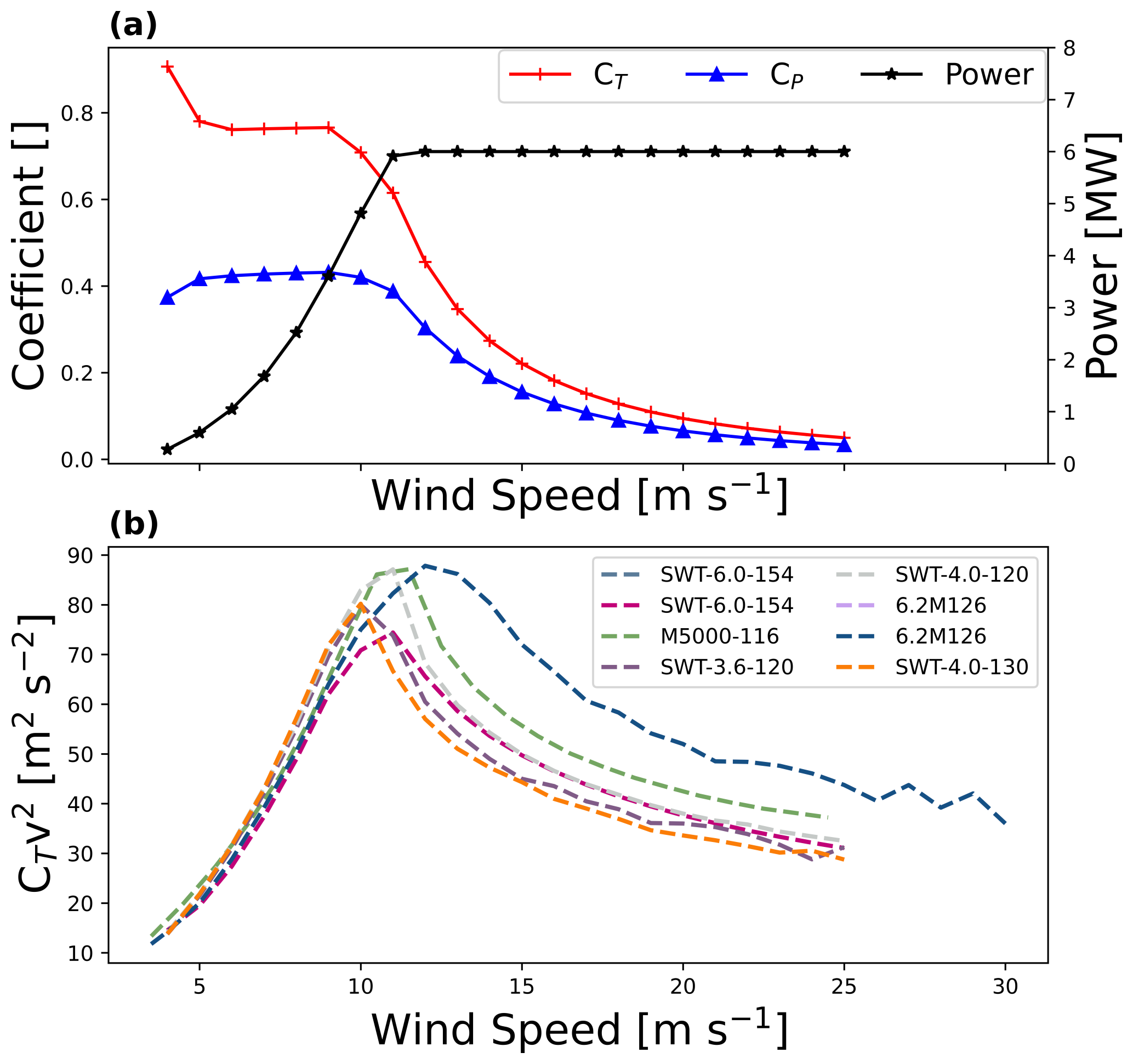
Figure 3 (a) Curve illustrating turbine C_T, C_P, and power specifications for the turbine model in the Gode wind farm. (b) Drag proxy for each of the eight turbine models present in this case study.

Table 6 Full set of WRF simulations and sensitivities. The simulations in bold are those formally evaluated for performance, and the simulations not in bold are sensitivity runs explored in the Appendix.

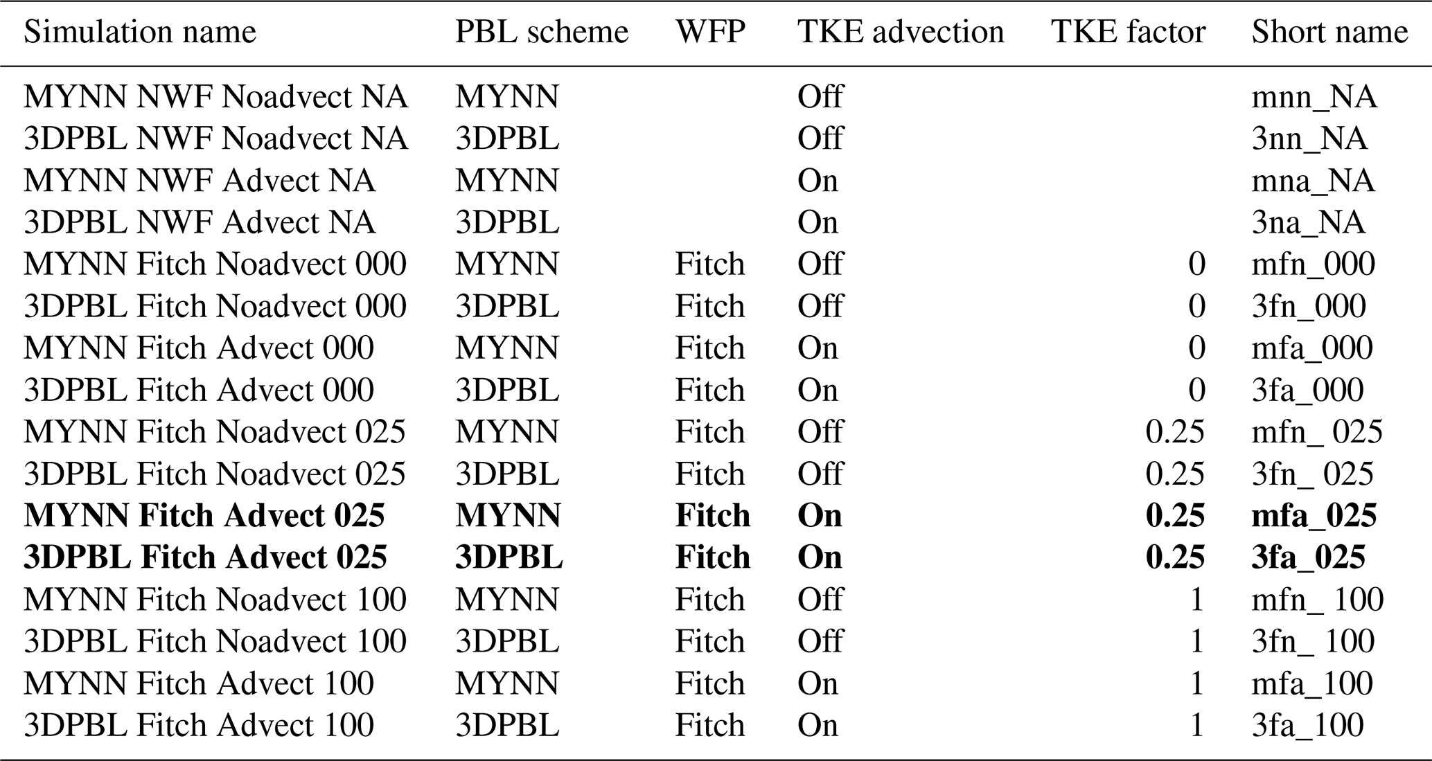
Our simulations varied the wind farm option, the wind farm TKE factor, and the advection option for each PBL scheme (Table 6). We highlight the results from the two simulations with the Fitch scheme, the advection option on, and the wind farm TKE factor of 0.25 to focus the scope on the effects of the PBL scheme (Table 6). The results from the other 14 runs are analyzed throughout the Appendix.

2.4 Model validation

2.4.1 Other diagnostic variables

We now describe other calculated quantities used to understand site performance and physical mechanisms.

The wind speed deficit, λ, characterizes wake strength:

$$\begin{array}{}\text{(10)}& {\mathit{\lambda }}_{ijk}=U_{{\mathrm{NWF}}_{ijk}}-U_{{\mathrm{Fitch}}_{ijk}},\end{array}$$

where $U_{{\mathrm{NWF}}_{ijk}}$ is the horizontal wind speed at a specific grid cell ij and specific height index k with no wind farms, and $U_{{\mathrm{Fitch}}_{ijk}}$ is the horizontal wind speed with the corresponding wind farm simulation.

The “drag proxy”, D, for a constant density and rotor area is given by

$$\begin{array}{}\text{(11)}& D=C_{\mathrm{T}}{V}^{\mathrm{2}},\end{array}$$

where C_T and V are the corresponding manufacturer-specified proper thrust coefficients and wind speeds, respectively (Figs. 3a, b).

ΔTKE represents the time-averaged difference in TKE between the two PBL schemes at a given i, j, and k location.

$$\begin{array}{}\text{(12)}& \mathrm{\Delta }\mathrm{TKE}={\mathrm{TKE}}_{\mathrm{3}\mathrm{DPBL}}-{\mathrm{TKE}}_{\mathrm{MYNN}}\end{array}$$

This difference field, consistent with all subsequent difference fields, is defined as 3DPBL − MYNN.

2.4.2 Spatial and temporal processing

Additional spatial and temporal averaging was applied, with care being taken to reflect site differences. For the FINO1 region, 10 min WRF output data for the hours of 12:00:00–00:00:00 UTC were averaged to compare with the FINO1 data. For the FINO1 region, the 10 min model output data were subset to the closest ij grid cell and k model level in relation to the 10 min observations. Each observational height was evaluated separately.

Additional processing was necessary to capture the temporal and spatial variability of the aircraft transect paths. Because each transect represented approximately 10 min of observations, each transect could be reasonably compared to a single 10 min model output. At the same time, observations within a single transect spanned multiple model grid cells. Given these additional considerations, we processed the aircraft region data with the following process, based on Platis et al. (2018) and Larsén and Fischereit (2021). First, we calculated the horizontal wind speed as follows:

$$\begin{array}{}\text{(13)}& U=\sqrt{u^{\mathrm{2}}+v^{\mathrm{2}}},\end{array}$$

where u and v are the zonal and meridional components, respectively, of the wind in m s⁻¹ for a given transect with the 100 Hz observations. Then, we resampled the horizontal wind speeds with a moving 2 km window. This 2 km window was first determined by Platis et al. (2018) and was later implemented in Larsén and Fischereit (2021) for this case study. This window was selected based on the aircraft speed to yield an average turbulent timescale on the order of a couple of minutes. This integral timescale appropriately separates the small-scale fluctuations from the large-scale turbulent motions (Platis et al., 2018; Larsén and Fischereit, 2021). Additional averaging was then performed, this time across grid cells. The 2 km resolution wind speed calculations were mapped to a corresponding model grid cell based on their latitude and longitude, and all of the 2 km resolution wind speed calculations for a given model grid cell were averaged together. The number of 2 km resolution wind speed calculations for a given model grid cell depended on the amount of time that the aircraft spent in that grid cell. Well-sampled grid cells may contain close to 3000 points, whereas less sampled grid cells may contain only 10 points. These grid-cell-averaged values could then be compared to the relevant model cell value at the closest time step (Table 2).

We employed a similar process to calculate TKE, also based on Platis et al. (2018) and Larsén and Fischereit (2021). We again isolated the 100 Hz observations for a given transect and resampled the TKE based on a 2 km moving (standard deviation) window (Platis et al., 2018):

$$\begin{array}{}\text{(14)}& \mathrm{TKE}={\displaystyle \frac{\mathrm{1}}{\mathrm{2}}}({\mathit{\sigma }}_u^{\mathrm{2}}+{\mathit{\sigma }}_v^{\mathrm{2}}+{\mathit{\sigma }}_w^{\mathrm{2}}),\end{array}$$

where σ_u, σ_v, and σ_w correspond to the standard deviations of the u, v, and w components, respectively. We then averaged these values across each grid cell to compare to the WRF model (Table 2).

Model data and observations from the aircraft vertical profiles were compared to assess the model's ability to capture important local characteristics like atmospheric stability. Because each profile traversed several model grid cells, observations for a given profile were compared to a designated “middle” model grid cell (Table 3). Potential temperature, θ [K], was calculated – both from the 100 Hz observations and from 10 min model data – according to the following equation:

$$\begin{array}{}\text{(15)}& \mathit{\theta }=({\displaystyle \frac{p_{\mathrm{0}}}{p}}{)}^{\mathrm{0.2854}},\end{array}$$

where p₀ is the reference pressure 10 000 hPa, and p (hPa) is the pressure surrounding the aircraft at a given moment. Horizontal wind speed and TKE for the aircraft profile observations were calculated using Eqs. (13) and (14), as used with the aircraft transect flights. However, the rolling-averaging window for the aircraft profile flights was 10 m (as opposed to 2 km), again, as in Larsén and Fischereit (2021).

These wind speed (and corresponding TKE) retrievals were subject to errors in aircraft yaw alignment. Bärfuss et al. (2023) analyzed experimental influences on retrievals from a drone platform and concluded yaw misalignment to be the dominant source of error for wind speed (and TKE) retrievals. Bärfuss et al. (2023) also noted that errors in yaw alignment have opposite signs depending on whether the sensor interacts with the wind from the starboard or backboard side. Because odd transects expose the sensor to one side of the plane and even transects expose the sensor to the other side, this error in yaw alignment could be reflected in systematic differences in wind speed (and TKE) between even transects and odd transects.

2.4.3 Error metrics

The standard (Optis et al., 2020) error metrics of bias, centered root mean square error (cRMSE), correlation squared (R²), and earth movers' distance (EMD) were calculated for each available variable at each site. The bias, cRMSE, and EMD all have an optimal value of 0, whereas R² has an optimal value of 1. For the FINO1 region, the averages represented time averages, and, for the aircraft region, the averages were across grid cells. FINO1 time averages included all 10 min data points for the 12:00:00–00:00:00 UTC period. The bias represents the difference between the modeled and observed means:

$$\begin{array}{}\text{(16)}& \mathrm{bias}=(\stackrel{\mathrm{‾}}{p}-\stackrel{\mathrm{‾}}{o}),\end{array}$$

where $\stackrel{\mathrm{‾}}{p}$ represents the modeled mean, and $\stackrel{\mathrm{‾}}{o}$ represents the observed mean. The cRMSE represents the unbiased component of the model error. The cRMSE, in this case, is as follows:

$$\begin{array}{}\text{(17)}& \mathrm{cRMSE}=\left[{\displaystyle \frac{\mathrm{1}}{N}}\sum _{n=\mathrm{1}}^N\right[(p_n-\stackrel{\mathrm{‾}}{p})-(o_n-\stackrel{\mathrm{‾}}{o}){]}^{\mathrm{2}}{]}^{\mathrm{1}/\mathrm{2}},\end{array}$$

where N is the number of data points. The Pearson correlation coefficient (R) represents the correspondence between two variables:

$$\begin{array}{}\text{(18)}& \mathrm{R}={\displaystyle \frac{\frac{\mathrm{1}}{N}{\sum }_{n=\mathrm{1}}^N\left[\right(p_n-\stackrel{\mathrm{‾}}{p})-(o_n-\stackrel{\mathrm{‾}}{o}\left)\right]}{{\mathit{\sigma }}_{\mathrm{p}}{\mathit{\sigma }}_{\mathrm{o}}}},\end{array}$$

where σ_p and σ_o represent the standard deviations of the predictions and observations, respectively. Here, we reported the coefficient of determination, R², as recommended in Optis et al. (2020). Finally, EMD, also known as the Wasserstein distance, represents the area between two cumulative distribution functions. The EMD can be described by the following:

$$\begin{array}{}\text{(19)}& \mathrm{EMD}(\mathrm{u},\mathrm{v})=\underset{\mathit{\pi }\in \mathrm{\Gamma }(u,v)}{inf}\underset{\mathbb{R}\times \mathbb{R}}{\int }|x-y|\mathrm{d}\mathit{\pi }(x,y),\end{array}$$

where Γ(u,v) is the set of probability distributions on ℝ×ℝ, whose marginals are u and v on the first and second factors, such that u(x) is the probability of u at position x, and v(x) is the probability of v at position x (Ramdas et al., 2015). Here, the EMD was calculated with the Python function wasserstein_distance() from the SciPy library (Virtanen et al., 2020).

2.4.4 Statistical significance testing

Statistical significance testing was also performed to determine the strength of the differences between simulations. This testing was performed for each error metric separately, with each transect and/or height representing a value of the appropriate sample. Noting the small number of data points, as well as the non-normality of each sample, we performed our statistical testing with a Mann–Whitney U test (Mann and Whitney, 1947). The Mann–Whitney U test is a non-parametric, rank-sum test that relaxes traditional normality and variance requirements with many other statistical tests. Tests were performed with the corresponding Python function from the SciPy stats module (Virtanen et al., 2020), and a result is deemed to be statistically significant if $\left|p\right|<\mathrm{0.05}$.

3 Results

We outline the results of the 3DPBL and MYNN evaluation below. We begin with an overall site characterization and then move to a consideration of the systematic influences of model influence and finish with a statistical evaluation of model performance at both sites.

3.1 Site characterization

3.1.1 Profiles of atmospheric variables

The modeled atmospheric stability both at the FINO1 location (Fig. 4a, b) and over the aircraft region (Fig. 4f, g) suggests a weakly stable profile near the surface with stronger stability aloft. MYNN simulations are slightly warmer (according to potential temperature) and more stable near the surface than 3DPBL simulations (Fig. 4b, g). For both sites, these modeled temperature profiles are consistent with available observations (Fig. 4a, f), and the observed potential temperature in the aircraft region is slightly warmer than the modeled potential temperature (Fig. 4g). Because the modeled air temperatures are almost identical between models (Fig. 4a, f), these slight differences in the surface stability could be a consequence of the greater TKE with the 3DPBL scheme that encourages slightly more mixing. The wind direction profiles at both FINO1 (Fig. 4c) and the aircraft transect (Fig. 4h) regions show veering wind (i.e., the wind direction rotates from southwesterly direction near the surface to westerly aloft), suggesting warm-air advection. Simulations with MYNN also tend to have slightly more southerly winds than simulations with the 3DPBL scheme (Fig. 4c, h). Wind speeds are similar near the surface and through the rotor layer, with slight variations between the aircraft and FINO1 regions (Fig. 4d, i). Peak wind speeds for both sites are slightly higher than the peak TKE, reflecting an LLJ, as in Larsén and Fischereit (2021). The wind direction vertical profiles for both the FINO1 (Fig. 4c) and aircraft (Fig. 4h) regions also suggest inversions at 500 m. Although this separate air mass would not be considered to be an inversion according to the potential temperature vertical profiles (Fig. 4a, d), the variation in wind speed does support a distinct layer above 500 m (Fig. 4d, i). Further, the modeled PBL height, which, under stably stratified conditions, is determined as the height at which the TKE profile reaches 5 % of its surface value (Olson et al., 2019), corroborates this distinction. Thus, dynamically, the top of the stable boundary layer likely resides around 500 m.

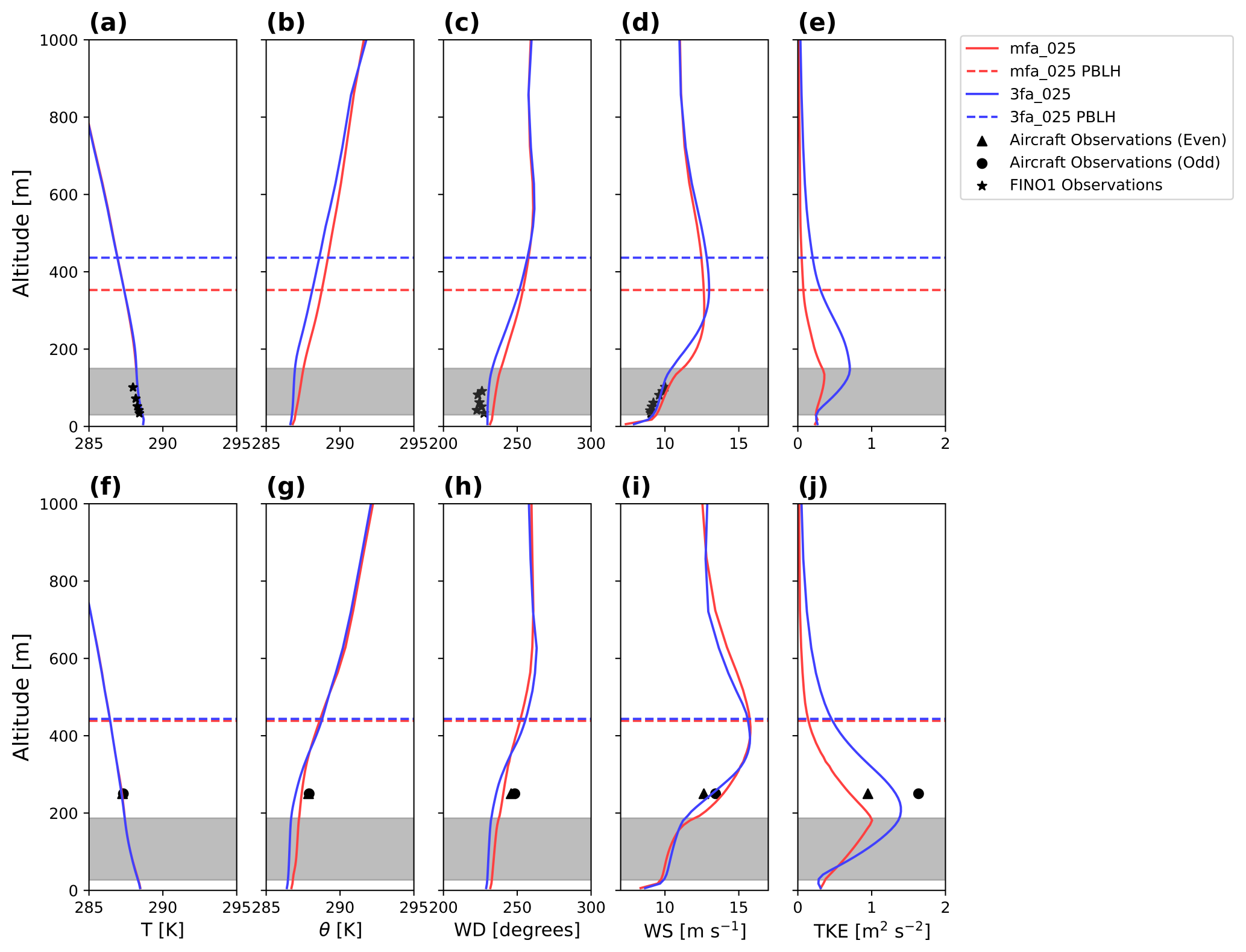
Figure 4 Temperature, potential temperature, wind direction, wind speed, and TKE vertical profiles from observations and WRF simulations for both sites. In all cases, the dashed lines indicate the modeled PBL height, and the gray region indicates the turbine rotor region. Observations in the aircraft region are separated between and even and odd transects. (a) FINO1 temperature, (b) FINO1 potential temperature, (c) FINO1 wind direction, (d) FINO1 horizontal wind speed, (e) FINO1 TKE, (f) aircraft temperature, (g) aircraft potential temperature, (h) aircraft wind direction, (i) aircraft horizontal wind speed, (j) aircraft TKE. FINO1 cases are averaged over the hours of 12:00:00–00:00:00, and the aircraft region cases are averaged over 14:10:00–16:10:00 UTC. FINO1 TKE calculations based on observations were not available due to the coarse temporal resolution of the wind speeds. FINO1 potential temperature calculations based on observations were not available due to a lack of pressure observations.

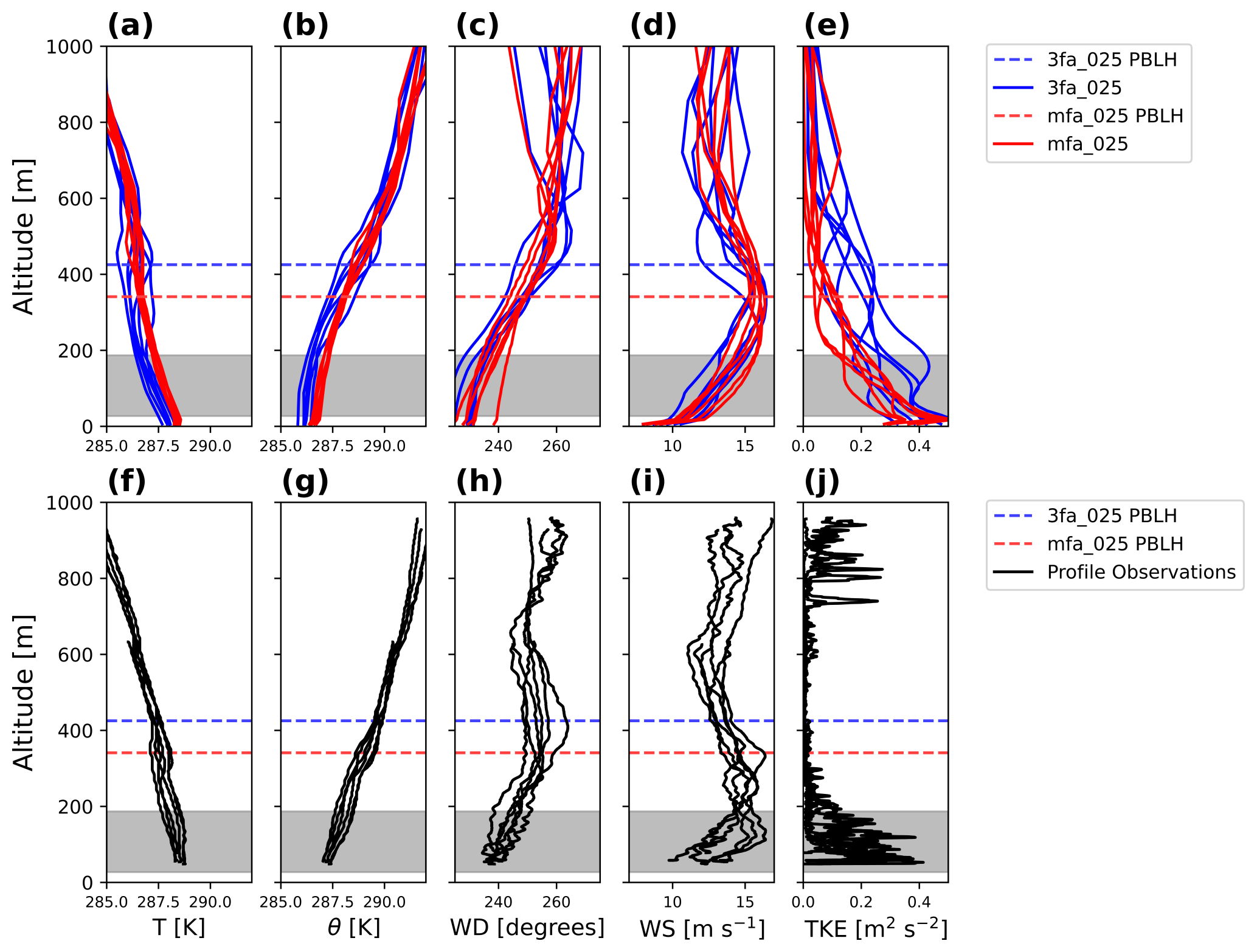
Figure 5 Observed and modeled vertical profiles for the aircraft vertical profile flights (Table 3, Fig. 1b). In all cases, the horizontal line indicates the modeled PBL height, and the color differentiates the PBL scheme. The top row of panels corresponds to modeled output, and the bottom row of panels corresponds to the aircraft profile observations. Modeled outputs are determined to be a given middle cell for each profile as in Larsén and Fischereit (2021) based on the time step indicated in Table 3. (a) Modeled temperature, (b) modeled potential temperature, (c) modeled wind direction, (d) modeled horizontal wind speed, (e) modeled TKE, (f) observed temperature, (g) observed potential temperature, (h) observed wind direction, (i) observed horizontal wind speed, (j) observed TKE.

The TKE peaks differentiate the two model vertical profiles at both sites. The 3DPBL TKE scheme is consistently larger beyond the surface, and this discrepancy is largest at and slightly above the rotor level. The fundamental differences in horizontal-mixing and length scales between the schemes lead the 3DPBL scheme to characterize more TKE. These differences are more accentuated with both an LLJ and the turbine-induced TKE contribution.

Simulated TKE also differs from observations. While MYNN TKE underpredicts TKE observed during both even and odd transects, the 3DPBL TKE overpredicts TKE during even transects and underpredicts TKE during odd transects. These deviations between modeled and observed TKE may, in part, reflect the model formulations. However, yaw (mis)alignment of the aircraft may also play a part in these discrepancies. The error in yaw alignment is expected to have alternating signs on whether the wind approached the sensor from the starboard or the backboard side (Bärfuss et al., 2023). Because the even and odd transects involved opposite alignments of the aircraft, it would follow that the odd and even transects would then show distinct TKE (and wind speed, on a smaller scale) errors. Thus, the discrepancy between TKE observed with the odd and even transects may also play a part in the poor model agreement.

3.1.2 Aircraft profile flights

The aircraft profile flights suggest a similar vertical structure to that for the FINO1 and aircraft transect regions. Both MYNN and 3DPBL temperature and potential temperature profiles at the locations of the profiles (Fig. 5a, b) suggest a weakly stable profile near the surface, with stronger stability aloft. This stability is reinforced by the aircraft profile observations (Fig. 5f, g). An LLJ once again emerges in both wind speed (Fig. 5d, i) and TKE (Fig. 5e, j) maxima. Finally, once again, both modeled (Fig. 5c) and observed (Fig. 5h) wind direction from the aircraft profiles suggest warm-air advection with an inversion that is supported by the modeled PBL height.

For the aircraft profile flights, the vertical structure suggests discrepancies between the model and observations in terms of both values and shape (Fig. 5). The wind direction (Fig. 5c, h) rotation is also modeled at a higher altitude than observed. The observed surface wind direction (Fig. 5h) also reflects an approximately 20° discrepancy from the modeled surface wind direction (Fig. 5c). Observed wind speeds (Fig. 5i) are also faster than modeled wind speeds (Fig. 5d), with an additional local peak lower than 200 m that is not captured by the model. Finally, observed TKE (Fig. 5j) suggests two peaks, with one peak within the turbine rotor layer and the other peak well above aircraft transect flights and the top of the boundary layer. In contrast, modeled TKE (Fig. 5c) suggests a single TKE peak with a more gradual decrease with height. These discrepancies in agreement could be explained by several factors, such as the larger number of available data points for the aircraft profile flights, a lack of a smoothing time average for the aircraft profile observations, and the spatial variability sampled with the aircraft profile flights.

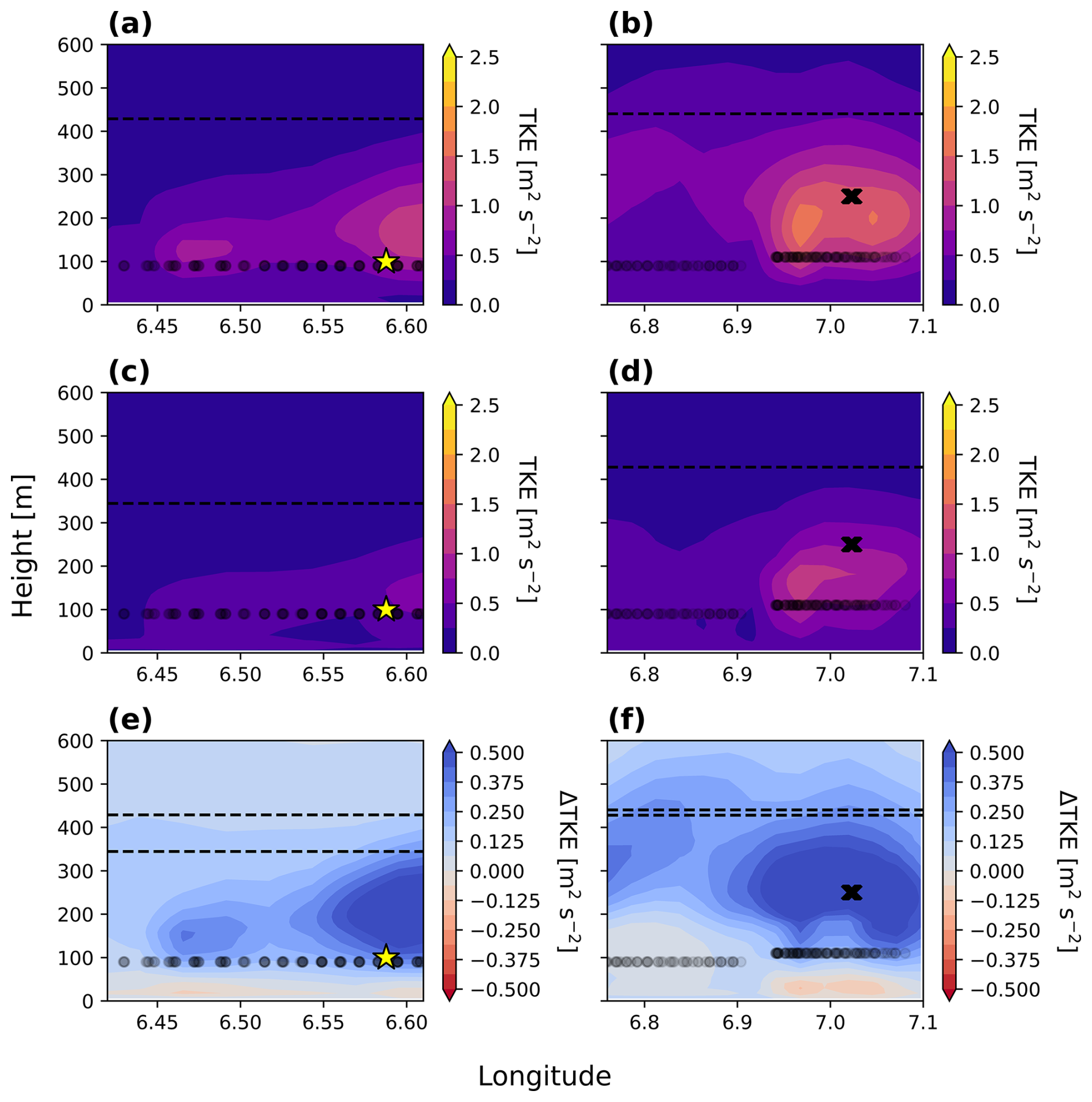
Figure 6 Modeled TKE cross-section at a constant latitude of 54.03. (a) FINO1 3fa_025, (c) FINO1 mfa_025, (e) FINO1 3fa_025 – mfa_025, (b) aircraft 3fa_025, (d) aircraft mfa_025, (f) aircraft 3fa_025 – mfa_025. The horizontal dashed black line denotes the average modeled PBL height, the star indicates the FINO1 tower location, the “X” marks the first transect path, and the black circles indicate the turbine hub height.

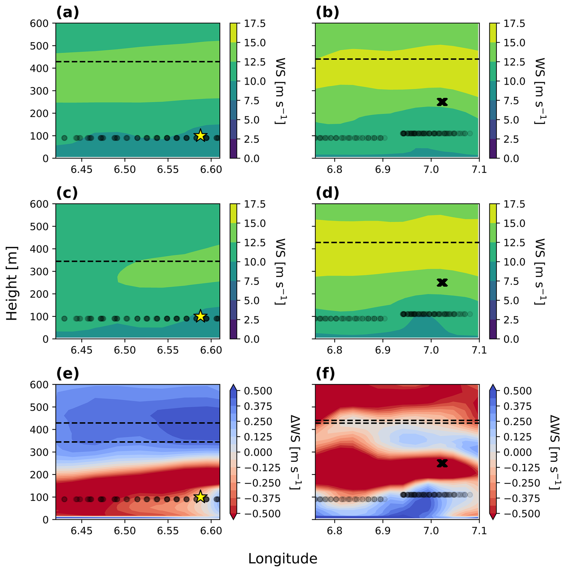
Figure 7 Modeled wind speed cross-section at a constant latitude of 54.03. (a) FINO1 3fa_025, (c) FINO1 mfa_025, (e) FINO1 3fa_025 – mfa_025, (b) aircraft 3fa_025, (d) aircraft mfa_025, (f) aircraft 3fa_025 – mfa_025. The horizontal dashed black line denotes the average modeled PBL height, the star indicates the FINO1 tower location, the “X” marks the first transect path, and the black circles indicate the turbine hub height.

3.1.3 Impacts of stable stratification

The stable stratification may suppress some of the turbine-generated turbulence from extending aloft. Both FINO1 and the aircraft transect measurement regions show simulated TKE peaks at altitudes within the rotor region due to wind-farm-generated turbulence. Both the FINO1 and aircraft regions also show larger amounts of TKE with the 3DPBL scheme (Fig. 6a, b) than with the MYNN scheme (Fig. 6c, d). These differences in TKE between the PBL schemes, which are consistent with those shown under the idealized, stable conditions simulated in Rybchuk et al. (2022), reflect the fundamental differences between the models. The stronger TKE maxima in the 3DPBL (Fig. 6a, b) at both sites also lead to greater interfarm TKE overlap with 3DPBL than for MYNN (Fig. 6c, d), such that the TKE interactions between the wind farms are more pronounced for 3DPBL. The difference in both the intensity and degree of overlap between the 3DPBL and MYNN TKE maxima is stronger in the aircraft region (Fig. 6f) than in the FINO1 region (Fig. 6e), likely due to the larger number of wind turbines in the aircraft region (Fig. 6a, c). However, whereas the aircraft region's simulation suggests a higher maximum TKE than the FINO1 region, not all of the aircraft region TKE is captured by the measurements (Fig. 6b, d). The turbine-induced turbulence is sampled well by the FINO1 tower (Fig. 6a, c). However, some of this turbine-induced turbulence is suppressed from reaching the aircraft region measurement height (Fig. 6b, d). The two PBL schemes also do not respond to this stable stratification in the same manner. The 3DPBL scheme simulates more of this TKE reaching the aircraft measurement height, resulting in a comparatively larger 3DPBL − MYNN TKE difference at the aircraft measurement height (Fig. 6f).

These diverging patterns in TKE characterization between the two sites also have secondary influences on measured wind speeds (Fig. 7). In the aircraft region, enhanced TKE implies greater momentum extraction and, consequently, reduced wind speeds at the measurement site (Fig. 7b, d, f). In the FINO1 region, however, TKE from aloft mixes more momentum from aloft into the measurement region, which increases wind speeds (Fig. 7a, c, e). Thus, the differing measurement altitudes between the two sites may impact both the TKE and wind speed assessments presented below.

3.1.4 Spatial variability

Wind field behavior near the turbines differs from that for the rest of the simulation domain on average. Recall that the 3DPBL scheme incorporates more potential sources of TKE generation. MYNN average wind speeds are faster than 3DPBL average wind speeds outside of the turbine wakes (Fig. 8a). These MYNN average wind speeds likely exceed 3DPBL average wind speeds in this area because the 3DPBL scheme generates more TKE (Fig. 8b) due to the fact that the 3DPBL turbulence parameterization includes more terms that allow for horizontal mixing. Because the atmospheric boundary layer experiences more TKE in the 3DPBL simulation, the frictional forces are slightly larger, reducing the horizontal winds in this stably stratified flow case. This larger TKE with the 3DPBL scheme extracts more momentum from the mean wind, resulting in a greater reduction in wind speeds. This finding that MYNN wind speeds are faster than 3DPBL wind speeds for the same forcing or boundary conditions is consistent with other comparisons of these two PBL schemes, completed under both real and idealized conditions (Juliano et al., 2022; Rybchuk et al., 2022; Arthur et al., 2022; Peña et al., 2023; Arthur et al., 2025). This finding is also documented further in Fig. 7 and in Sect. A1. Note that this increased TKE in the 3DPBL scheme is particularly evident along the Danish coast, resulting in even slower winds in the 3DPBL scheme (Fig. 8a, b).

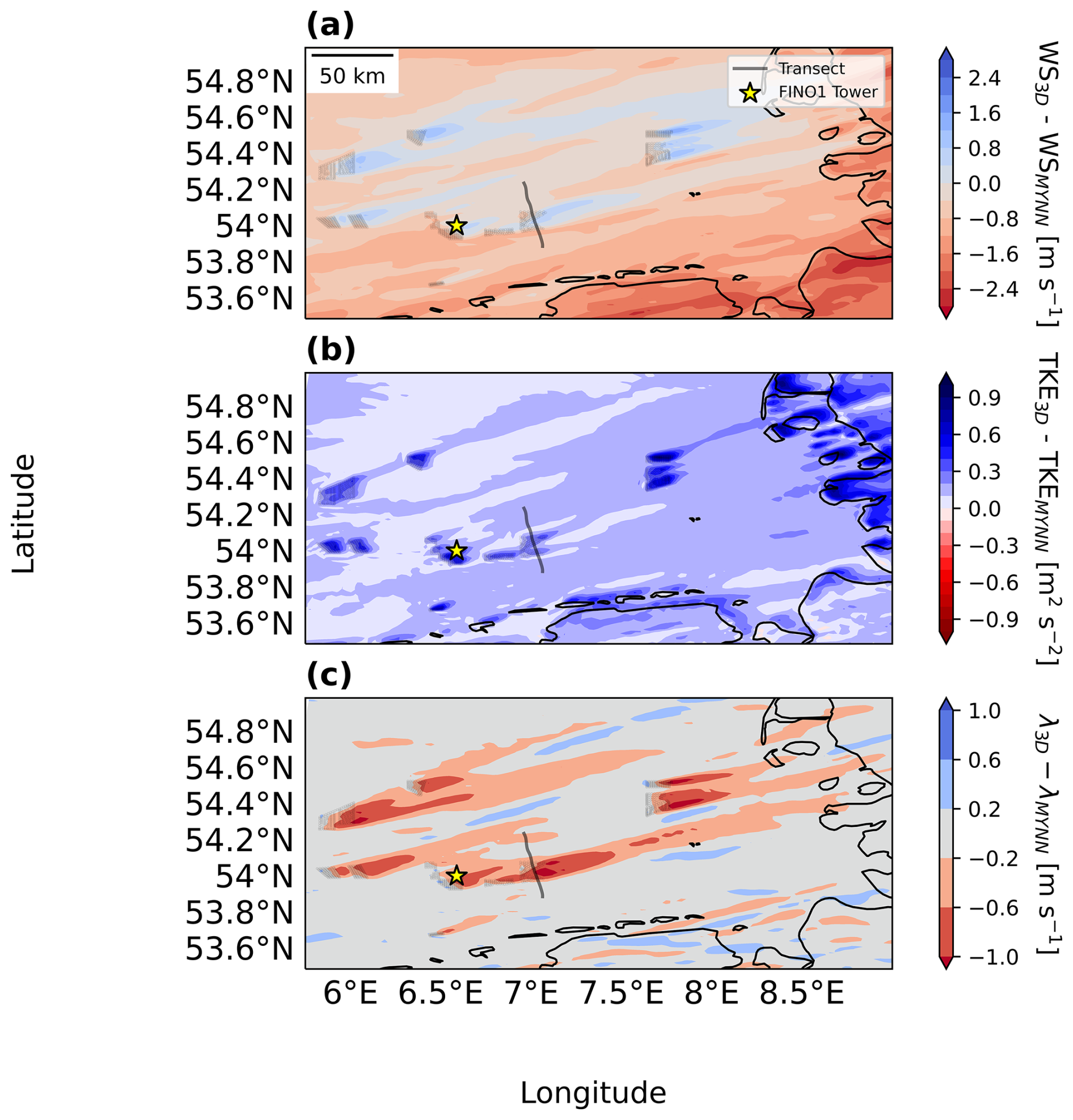
Figure 8 Difference fields for inner region at a 100 m hub height: (a) 3fa_025 – mfa_025 WS, (b) 3fa_025 – mfa_025 TKE, (c) 3fa_025 – mfa_025 wake deficit. Turbines are marked with black circles, the FINO1 tower is marked with a yellow star, and the first transect path is marked with a solid line.

Once these faster winds, in the MYNN scheme, enter the region of a wind farm, the faster winds lead to a larger drag force exerted by the wind turbines (Fig. 3b) and therefore a larger wake effect, resulting in slower winds in the MYNN wakes (Fig. 8a). This distinct behavior in the wakes arises from differences in the drag forces for each PBL scheme. The drag forces are very sensitive to wind speed (Fig. 3b). Because the MYNN wind speeds are slightly faster when entering the wind farms, the resulting MYNN drag force (Eq. 11, Fig. 3b) is generally larger than the 3DPBL drag force. As a consequence, the MYNN scheme shows stronger and longer wakes than the 3DPBL scheme, on average (Fig. 8c). The MYNN average wind speed reduction is sufficiently strong such that 3DPBL average wind speeds exceed MYNN average wind speeds within the turbine wake (Fig. 8a). Further, because 3DPBL average wind speeds exceed MYNN average wind speeds in this region, the 3DPBL scheme also has more turbine-induced TKE than the MYNN scheme (Fig. 8b). This turbine-induced TKE can help erode the wake in the 3DPBL simulations.

This behavior emerges fundamentally because of the difference in ambient background turbulence between the 3DPBL scheme and the MYNN scheme under these stably stratified conditions. Other behavior would manifest in stably stratified conditions if winds exceeded the wind speed of the peak drag force (near 13 m s⁻¹ in Fig. 3b), such that faster winds would result in a smaller drag force.

3.2 Measurement variability

3.2.1 FINO1 tower

Simulations capture the slowing winds observed at FINO1. Modeled FINO1 Fitch wind speeds appropriately capture the temporal shifts throughout the observational period (Fig. 9).

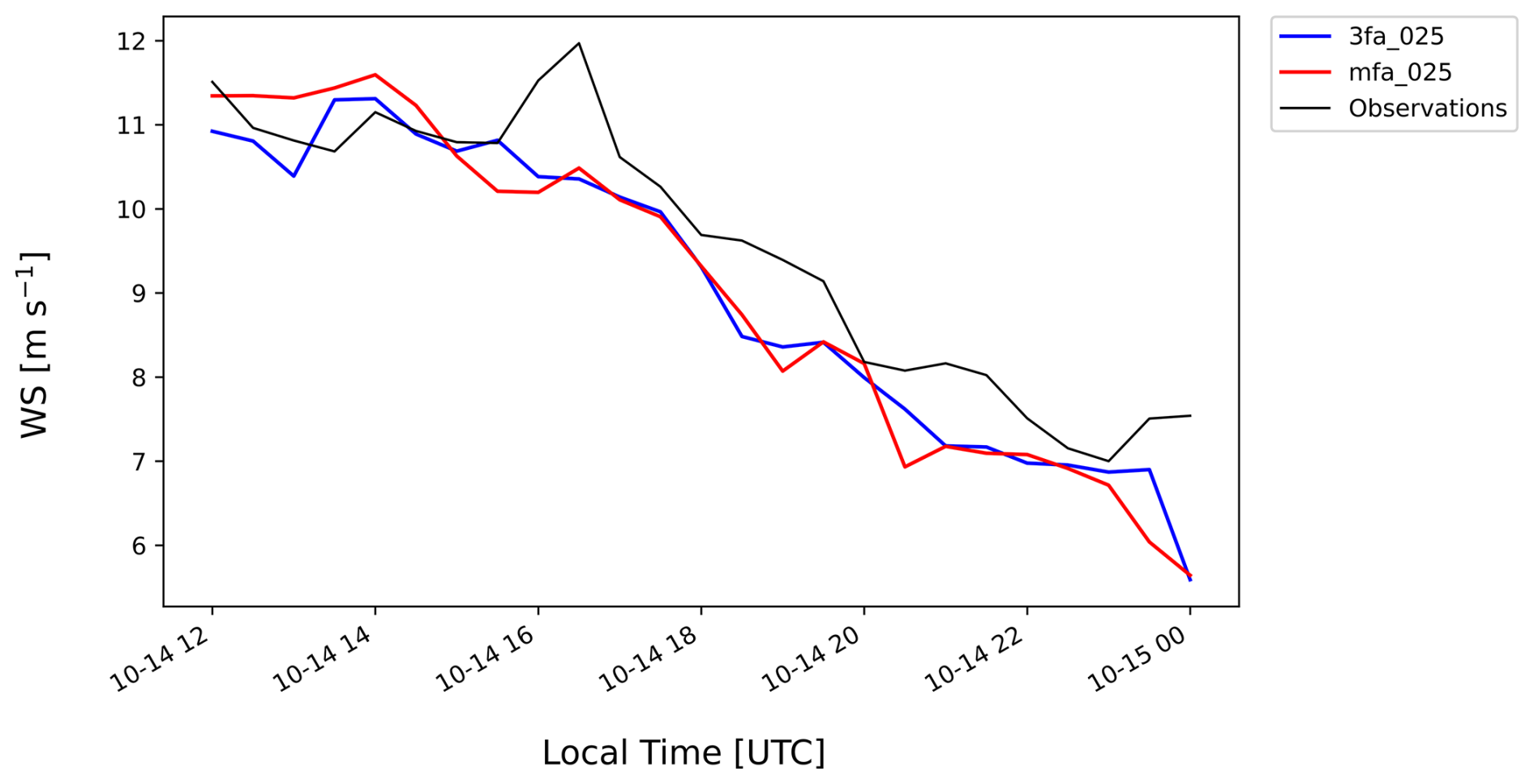
Figure 9 Time series of 76 m modeled horizontal wind speeds (WS) compared to 81 m FINO1 observations for the hours of 12:00:00–00:00:00 UTC. Both the modeled wind speeds and observed wind speeds are resampled to 30 min.

Observational agreement for FINO1 modeled wind speeds differs by measurement altitude. The median FINO1 modeled wind speeds at the highest locations (81, 91, and 102 m) perform best (compared to those at the lower altitudes of 34, 41, 51, and 61 m) for R² (Fig. 10b) and cRMSE (Fig. 10c) and the worst for the bias (Fig. 10a) and EMD (Fig. 10d). The low (34 and 41 m) and middle (51 and 61 m) heights show similar performance for the bias (Fig. 10a), R² (Fig. 10b), and EMD (Fig. 10d), with some additional shaping to the cRMSE (Fig. 10c). Further, the wind speeds at lower altitudes are also slower, resulting in smaller bias. Whereas 3DPBL EMD shifts from outperforming MYNN EMD at the low and middle heights to underperforming compared to MYNN EMD for the higher heights, the physics-based trends are consistent across the FINO1 model heights, which are stronger than the variability between heights. The 3DPBL cases consistently show larger wind speed biases (Fig. 10a) and smaller wind speed cRMSE (Fig. 10c) than the MYNN cases.

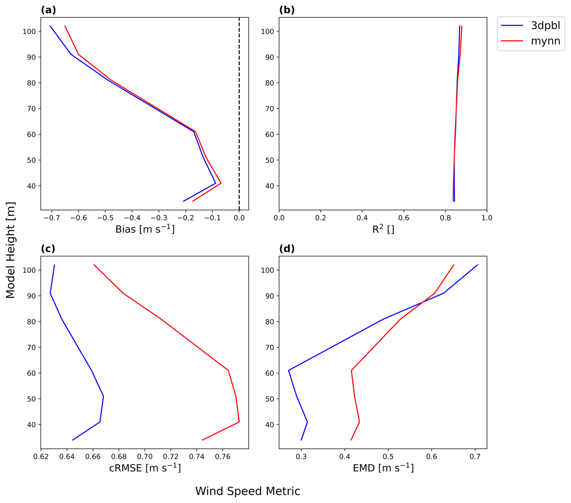
Figure 10 Error metric profile plot for FINO1 region wind speeds across all Fitch simulations with advection on and a wind farm TKE factor of 0.25. (a) Bias, (b) R², (c) cRMSE, (d) EMD.

3.2.2 Aircraft region

Similar patterns emerge for the wake-affected region of the flight path. The general trends of increased TKE (Fig. 11a) and decreased wind speed (Fig. 11b) above the wind farm clearly emerge. TKE in the wake portion of the flight path is simulated to be stronger in the 3DPBL simulations than in the MYNN simulations (Fig. 11a), and the maximum value in the 3DPBL simulations is similar to the maximum value in the observations, although the location of the TKE maximum is shifted downwind in both simulations. As noted earlier, these differences in TKE between the PBL schemes reflect the fundamental differences between the models in length scales, empirical constants, and horizontal-mixing approaches. Because the 3DPBL scheme has higher TKE, the 3DPBL scheme consequently shows slower wind speeds (Fig. 8b, 11a).

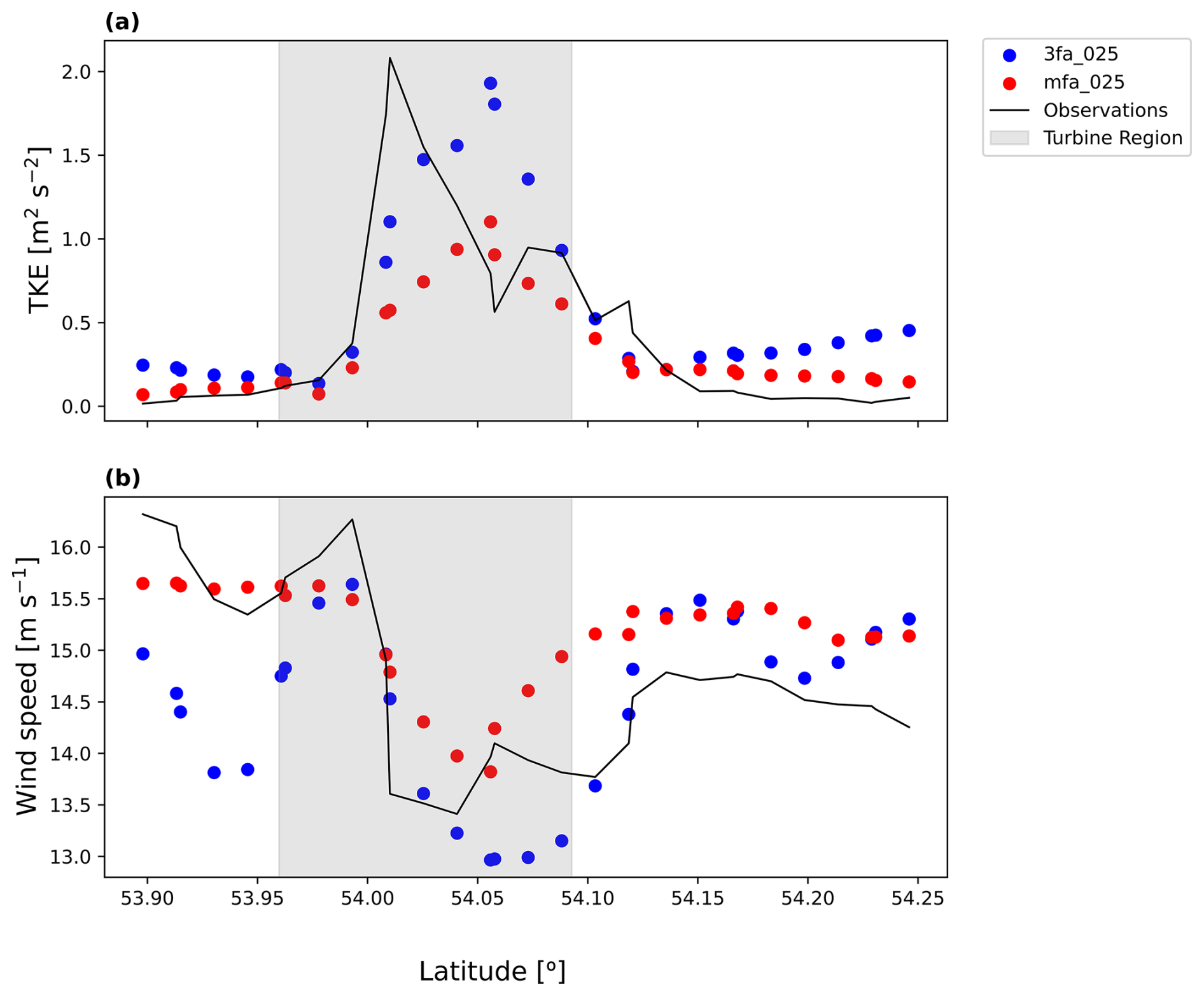
Figure 11 Aircraft region (250 m) simulated and observed (a) TKE and (b) wind speed across the flight path for transect 1. The shaded region incorporates the minimum and maximum latitudes of the turbine locations.

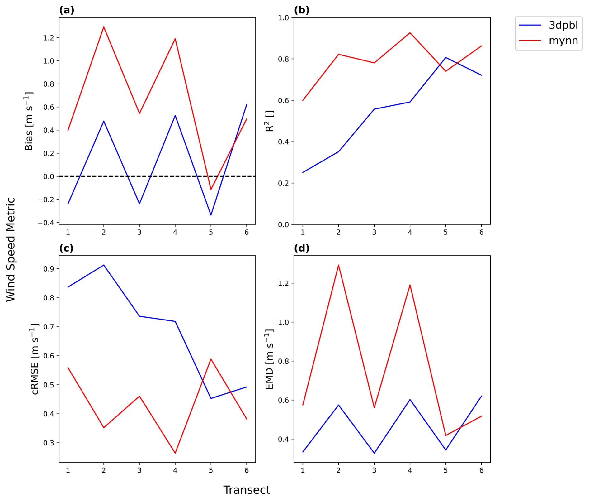
Figure 12 Error metric boxplot by transect for aircraft region wind speeds across all Fitch simulations with advection on and a wind farm TKE factor of 0.25. (a) Bias, (b) R², (c) cRMSE, (d) EMD.

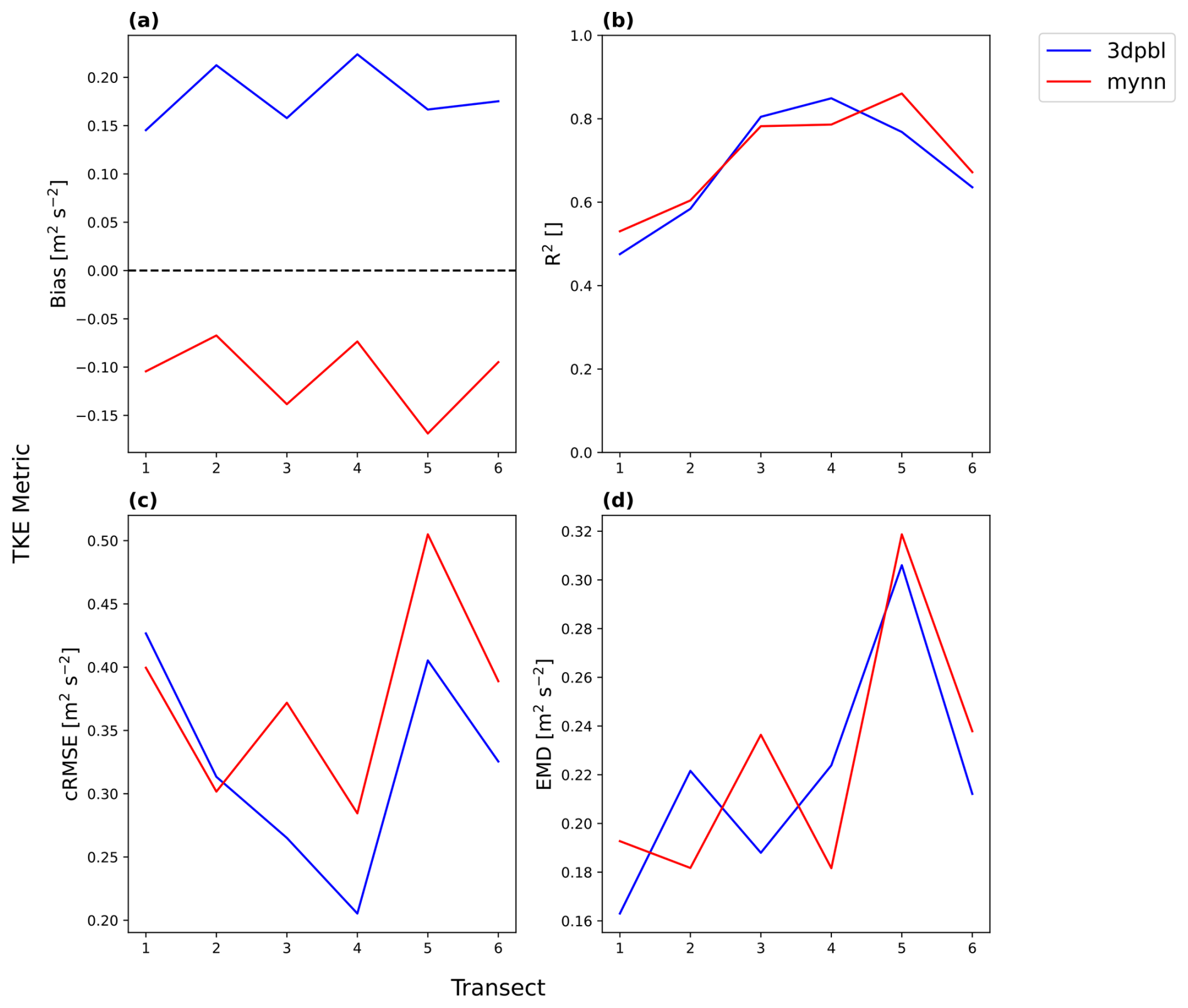
Figure 13 Error metric plot by transect for aircraft region TKE across all Fitch simulations with advection on and a wind farm TKE factor of 0.25. (a) Bias, (b) R², (c) cRMSE, (d) EMD.

Simulated aircraft region wind speeds and TKE are also subject to systematic influences between transects. First, a performance discrepancy between odd and even transects exists. Simulated wind speeds and TKE for southeast-to-northwest transects (1, 3, and 5) have a larger bias and EMD than those for northwest-to-southeast transects (2, 4, and 6) (Figs. 12a, d and 13a, d). This systematic transect variability corresponds to the reversed directions of the transect paths – whereas transects 1, 3, and 5 are performed in the northwesterly direction, transects 2, 4, and 6 are performed in the southeasterly direction.

This directional variability could potentially be explained by errors in yaw alignment. As noted earlier, the dominant source of error in one set of wind speed retrievals was previously determined to be the yaw measurements (Bärfuss et al., 2023). The error in yaw alignment was also determined to have alternating signs on whether the wind approached the sensor from the starboard or the backboard side (Bärfuss et al., 2023). Because the even and odd transects involved opposite alignments of the aircraft, it would follow that the odd and even transects would then show distinct wind speed (and TKE) errors.

Wind speed and TKE cRMSE and R² in the aircraft region also reveal additional systematic influences. While the transect direction does suggest an influence on these error metrics (Figs. 12b, c and 13b, c), these error metrics (cRMSE and R²) (Figs. 12b, c and 13b, c) additionally suggest an improvement over time that is not evident with the bias or the EMD (Figs. 12a, d and 13a, d). This performance improvement occurs after transect 2 and continues until transect 4 or 5 and is most evident from the R², although it does extend to the cRMSE, especially for the 3DPBL (Figs. 12c, 13c).

4 Model evaluation

A primary goal of this effort is to explore how simulated wake behavior changes based on the PBL scheme. The optimal PBL scheme depends on the site, error metric, and variable considered. The statistical significance of these differences, however, is more constrained. A statistically significant difference between 3DPBL and MYNN exists for wind speeds at the FINO1 site according to the cRMSE (Fig. 14d) but not for the bias (Fig. 14a), R² (Fig. 14g), or EMD (Fig. 14j). TKE in the aircraft region also shows a statistically significant difference for a single metric – in this case, the bias (Fig. 14c). In contrast, a statistically significant difference between 3DPBL and MYNN is present for all four metrics within the aircraft region (Fig. 14b, e, h, k).

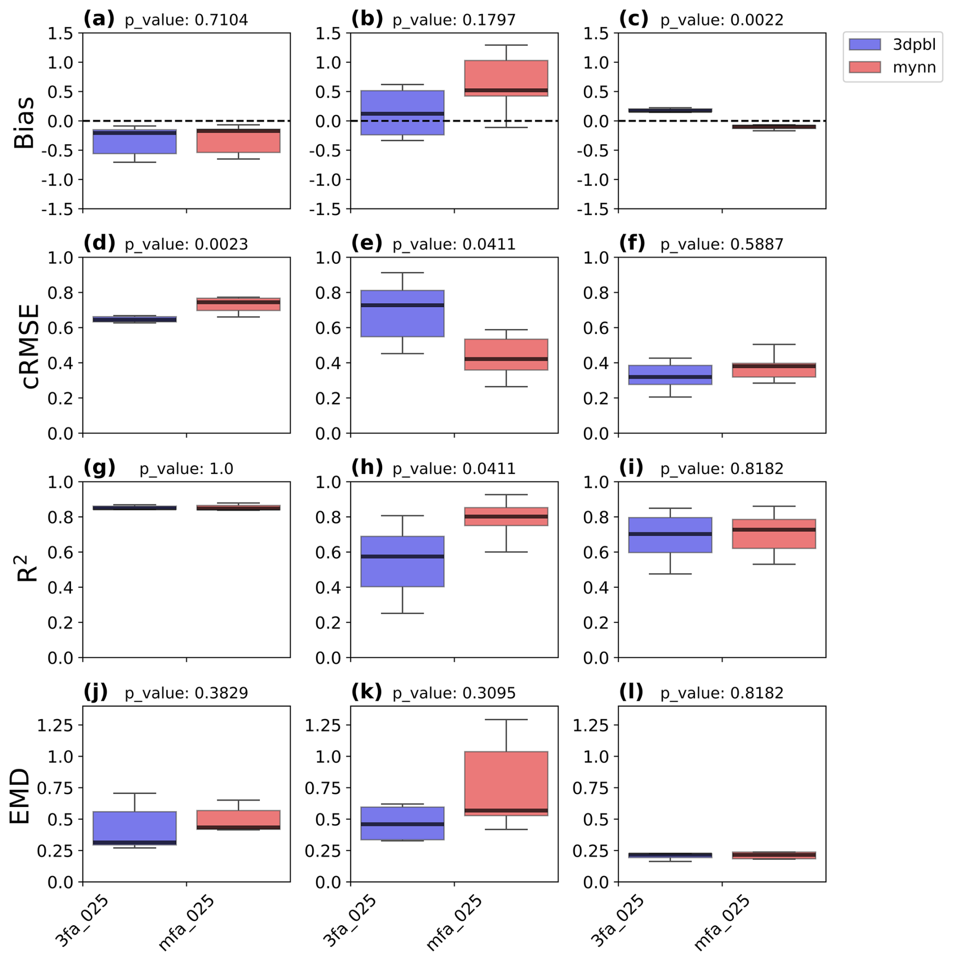
Figure 14 Error metrics across all Fitch simulations with the advection option on and with a wind farm TKE factor of 0.25. The first column corresponds to FINO1 wind speed error metrics, the second column corresponds to aircraft wind speed error metrics, and the third column corresponds to aircraft TKE error metrics. The bar indicates the median, the box encloses the interquartile range (IQR), and the whiskers extend to $\mathrm{Q}\mathrm{1}-\mathrm{1.5}\times \mathrm{IQR}$ and $\mathrm{Q}\mathrm{3}+\mathrm{1.5}\times \mathrm{IQR}$. Units are non-normalized and reflect the units of the evaluated field. (a) FINO1 wind speed bias [m s⁻¹], (b) aircraft wind speed bias [m s⁻¹], (c) aircraft TKE bias [m² s⁻²], (d) FINO1 wind speed cRMSE [m s⁻¹], (e) aircraft wind speed cRMSE [m s⁻¹], (f) aircraft TKE cRMSE [m² s⁻²], (g) FINO1 wind speed R² [ ], (h) aircraft wind speed R² [ ], (i) aircraft TKE R² [ ], (j) FINO1 wind speed EMD [m s⁻¹], (k) aircraft wind speed EMD [m s⁻¹], (l) aircraft TKE EMD [m² s⁻²]).

In the FINO1 region, 3DPBL wind speeds outperform MYNN wind speeds in representing wind speeds with respect to cRMSE (Fig. 14d), while the bias (Fig. 14a), R² (Fig. 14g), and EMD (Fig. 14j) are comparable between the PBL schemes. In contrast, the MYNN scheme holds a more decisive lead in comparison to observations collected 250 m above the surface and 100 m above a wind farm. MYNN TKE outperforms 3DPBL TKE with respect to bias (Fig. 14c), with no clear winner for cRMSE (Fig.  14f), R² (Fig. 14i), or EMD (Fig. 14l). For wind speeds evaluated with the aircraft dataset, MYNN outperforms 3DPBL with respect to cRMSE (Fig. 14e) and R² (Fig. 14h), whereas 3DPBL outperforms MYNN with respect to bias (Fig. 14b) and EMD (Fig. 14k).

The swapped bias performances between wind speed and TKE in the aircraft region may reflect competing optimizations. The TKE bias differs in sign between the two PBL schemes. The 3DPBL scheme overpredicts TKE (Fig. 14c), while the MYNN scheme underpredicts TKE (Fig. 14b). This higher TKE with the 3DPBL scheme implies that the 3DPBL scheme also has slower average wind speeds than the MYNN scheme (Figs. 8a and 11a, b). These slower average wind speeds imply an artificially improved wind speed bias (Fig. 14b). While the 3DPBL TKE overprediction improves wind speed performance on average, this performance enhancement does not necessarily imply other wind speed error metrics. Notably, the MYNN scheme outperforms the 3DPBL scheme with respect to both wind speed cRMSE (Fig. 14e) and wind speed R² (Fig. 14h). The role of TKE overpredictions in wind speed optimizations is further demonstrated in Sect. A2.

Previous studies have also found that the optimal PBL scheme depends on site and metric constraints. Draxl et al. (2014) found that the optimal PBL scheme depended on the atmospheric stability in an analysis of the Høvsøre wind farm. Hahmann et al. (2020) found that the MYNN scheme outperformed the Yonsei University (YSU) scheme in weekly simulations that used spectral nudging in characterizing eight sites in northern Europe. Hahmann et al. (2020) also performed a series of 25 simulations to compare PBL schemes, land surface models, and surface layer options and found that the differences between the sites were larger than the differences between PBL schemes, regardless of the error metric. Sheridan et al. (2024) found that the MYNN-based dataset both identified more of the extremely LLJ events and had a higher rate of false LLJ identification than the YSU-based dataset in the North Atlantic. Storm et al. (2009) similarly forecast LLJs in the Great Plains and found that, although the YSU scheme outperformed the Mellor–Yamada–Janjic (MYJ) PBL scheme in forecasting the wind direction, the MYJ scheme outperformed the YSU scheme with respect to wind speed for the same western Texas case. Storm et al. (2009) interpret these differences to be largely site-dependent and argue that the results would likely be different at another site. Olsen et al. (2025) analyzed LLJs from mast and lidar measurements in the North and Baltic seas by varying several modeling parameters including grid cell spacing, surface layer parameterizations, PBL schemes, and vertical resolution. Olsen et al. (2025) found that the PBL scheme was the most significant parameter in determining model results and that the 3DTKE scheme performed better than the other schemes considered.

Our results highlighting the advantages of the 3DPBL scheme within the turbine rotor layer are also supported by previous MYNN and 3DPBL intercomparisons. Arthur et al. (2022) found that the 3DPBL scheme consistently outperformed the MYNN scheme for a Columbia River Gorge site. Similarly, Arthur et al. (2025) compared the MYNN and 3DPBL schemes for an Altamont Pass site and also found the 3DPBL scheme to reduce wind speed error. Our cRMSE results in the turbine rotor layer align with those of Arthur et al. (2022) in that they both support the 3DPBL scheme over the MYNN scheme under stably stratified conditions. Our results also align with those of Arthur et al. (2025) in that they both show the 3DPBL scheme outperforming the MYNN scheme within the turbine rotor layer. Notably, whereas Arthur et al. (2022) and Arthur et al. (2025) were both performed in areas of complex terrain, which has been theorized to provide a theoretical advantage to the 3DPBL scheme (Kosović et al., 2020; Juliano et al., 2022), this work considers the relatively homogeneous offshore area, suggesting that the advantages of the 3DPBL scheme are not confined to complex terrain.

Grid cell spacing may influence the PBL comparison in this work. Notably, the 3DPBL scheme is theorized to improve model performance in the “terra incognita”, where the NWP horizontal grid spacing Δx approaches a similar magnitude compared to the PBL depth z (Wyngaard, 2004). Indeed, Arthur et al. (2022) found that the 3DPBL scheme outperformed the MYNN scheme in their simulations with a large-eddy simulation (LES) grid that has a finer cell spacing than that used in our mesoscale simulations. Thus, the mesoscale grid cell spacing necessary for this analysis, while vital to contextualize the results of this work with the broader literature, may restrict the potential benefits of the 3DPBL scheme over the MYNN scheme. At the same time, Peña et al. (2023) compared 3DPBL and MYNN to LES output and found that MYNN outperformed 3DPBL when the finest grid cell spacing was used. Thus, grid cell spacing may influence – but not necessarily dictate – the optimal PBL scheme.

Differences in the relative measurement height between the two sites in this case study may also affect the PBL comparison. Whereas the FINO1 tower is within the turbine rotor region, the aircraft measurements are taken more than 100 m above the turbines in a stably stratified boundary layer (Fig. 4) that suppresses some interactions between the atmosphere sampled at the turbine level and the aircraft level (Fig. 6). Thus, the 3DPBL scheme improves cRMSE turbine-induced turbulence characterization in the turbine rotor region as sampled at FINO1 (Fig. 14d) and overpredicts turbine-induced turbulence aloft as sampled by the aircraft measurements, on average (Fig. 14c).

The stable stratification present in this case study also improves the utility of the results of this PBL comparison. By restricting this analysis to time periods considered in previous analyses for this case study, the results contextualized within the broader literature, and the conditions that contribute the strongest and longest wakes are also highlighted. Thus, while other analyses of this region may approach the lack of available in situ observations by introducing statistical downscaling methods to explore scientific questions around diurnal, seasonal, and climatic trends (Fischereit et al., 2022b), this analysis instead addresses scientific questions that are best suited to in situ observations alone.

Other site-based considerations are less likely to be driving the relative PBL performance trends. The documented even–odd-transect variability (Figs. 12, 13) is not likely to drive the PBL-based differences given that the PBL-based differences are larger than the transect variability. The PBL-based preferences are also reinforced at all heights of the FINO1 tower (Fig. 9a, c, e), even despite performance variability between FINO1 heights (Fig. 10).

5 Conclusions

This work addresses PBL model capabilities for representing wind farm wakes with the Fitch WFP in the WRF model. This question underpins an important and understudied sensitivity of the NWP models that support both wind power forecasting and wind energy assessment. This work explores this question as one of the first comparative evaluations between the 1D MYNN PBL scheme and the newly Fitch-integrated NCAR 3DPBL scheme against two sets of in situ observations for an offshore case study.

The optimal PBL scheme depends on the site, variable, and error metric. For wind speeds modeled at the site within the turbine rotor region, 3DPBL outperforms MYNN with respect to the cRMSE. In contrast, for TKE modeled within a region 100 m above a wind farm, MYNN outperforms 3DPBL with respect to the bias. Ambiguously, for wind speeds modeled within the region 100 m above a wind farm, MYNN wind speeds outperform 3DPBL wind speeds with respect to R² and cRMSE but underperform with respect to bias and EMD. These site-based differences in the optimal PBL scheme likely reflect differences in the relative measurement height between the two sites. Whereas the FINO1 observations are collected within the turbine rotor region, the aircraft observations are collected 100 m above the turbine rotor layer, such that interactions between the turbine-induced turbulence and the aircraft measurements may be constrained by a stable boundary layer. Thus, 3DPBL simultaneously more appropriately characterizes behavior within the turbine rotor layer and overpredicts the amount of TKE reaching the aircraft region site.

Subsequent investigations could explore other case studies to provide perspective into the generalizability of the results across other sites. Similarly, datasets from the third Wind Forecast Improvement Project (WFIP3) could be useful to explore how offshore wind characterization might differ between the North Sea and the eastern United States (Kirincich et al., 2026). Moreover, datasets from the land-based, horizontally homogeneous American WAKE experimeNt – or AWAKEN – campaign (Moriarty et al., 2024) could be useful to study because previous land-based studies analyzing the 3DPBL scheme have involved complex terrain and far fewer detailed observations.

Further, this study focuses on simulations of the atmosphere alone, without coupling to the ocean surface or the water below. Another example of future work may include performing this analysis with an ocean model coupling (Raghukumar et al., 2022, 2023; Daewel et al., 2022). Although introducing a coupled ocean–atmosphere model does not always improve performance (Gaudet et al., 2024), introducing ocean coupling into this model could help diagnose sources of wind speed error for this model. Introducing a coupled ocean–atmosphere model also provides physical insight by potentially affecting the relative performance between the PBL schemes. Introducing ocean coupling also provides a more direct comparison to the work of Larsén et al. (2024), which included atmosphere–wave coupling, for this case study. Recreating this analysis with an additional ocean model like the Regional Ocean Modeling System (Shchepetkin and McWilliams, 2005) could provide insight into the influence of oceanic forcings on wind wake behavior and the resulting consequences on surface currents.

Power generation analyses for this case study are another future work opportunity. Analyses like those of Mittelmeier et al. (2017) and Sanchez Gomez et al. (2024) have demonstrated the utility of the available North Sea SCADA data in informing cluster wake research. As such, an accompanying analysis that validates the power estimates derived with each PBL scheme for this region may offer additional insight into model differences and draw interest from a broader set of stakeholders.

Appendix A: Additional simulation comparisons

A1 Contrast between NWF and WF options

Average wind speeds for the Fitch and NWF cases are similar in regions without wind turbines and differ near the turbines. Both NWF (Fig. A1a, c) and Fitch (Fig. A1b, d) average wind speeds are slower over land than over water. Further, the fastest average wind speeds are immediately to the west of the coast for both the NWF (Fig. A1a,c) and Fitch (Fig. A1b, d) cases. The predominant westerly wind direction and the significant distance of the measurement regions from the coast demonstrate that the measurement regions are not influenced by the coastal decelerations. MYNN average wind speeds (Fig. A1c,d) are also consistently faster than 3DPBL average wind speeds (Fig. A1a, b) for both NWF and Fitch cases outside of the turbine wakes (Fig. A1e, f). This difference in wind speeds between the PBL schemes can be explained by TKE differences between the two PBL schemes. Because the 3DPBL scheme has larger TKE (Fig. 8b), the 3DPBL scheme extracts more momentum and reduces wind speeds further. In contrast, Fitch and NWF wind speeds differ near the turbines. Notably, 3DPBL Fitch average wind speeds exceed MYNN Fitch average wind speeds in the turbine wakes (Fig. A1f). This reversal of which PBL scheme shows the faster average wind speed can be explained by differences in the turbine drag force between the two PBL schemes. The MYNN scheme has a stronger turbine drag force (Eq.  11, Fig. 3b) because of its faster initial wind speeds, which also implies that the MYNN scheme has stronger and deeper wakes (Fig. 8c). This reversal (of which PBL scheme shows the faster average wind speed) occurs only in the monotonically increasing region of the drag (proxy) curve (Fig. 3b). If the wind speeds were instead within the monotonically decreasing region of the drag (proxy) curve (Fig. 3b), MYNN wind speeds would likely exceed 3DPBL wind speeds even in the wakes because the faster winds would result in a smaller drag force (Fig. 3b). Given that NWF wind speeds mirror Fitch wind speeds outside of the turbine wakes and NWF wind speeds differ from Fitch wind speeds within the wakes, the dominant mechanism for these differences is more likely to be related to the turbines and not to the underlying meteorology.

A2 Effect of wind farm TKE factor, C_TKE

Recent scientific discussion (Mangara et al., 2019; Archer et al., 2020; Siedersleben et al., 2020; Sanchez Gomez et al., 2024; Ali et al., 2023; García-Santiago et al., 2024; Optis, 2024) has focused on the determination of the optimal value of the wind farm TKE factor, C_TKE, with varying conclusions. Several works corroborate improved performance with increased C_TKE. Vanderwende et al. (2016) found that Fitch simulations with a wind farm TKE factor of 0 underpredicted TKE. García-Santiago et al. (2024) similarly showed that the Fitch scheme could improve TKE underpredictions. Siedersleben et al. (2020), Ali et al. (2023), and Sanchez Gomez et al. (2024) also identified improved predictions with larger C_TKE. However, the overestimation of C_TKE is also evident in the literature. Vanderwende et al. (2016) likewise found that a wind farm TKE factor of 1 contributed to TKE overpredictions. Similarly, García-Santiago et al. (2024) found that the Fitch scheme with a wind farm TKE factor of 1 overpredicted TKE. Mangara et al. (2019) and Larsén et al. (2024) likewise identified excess TKE predictions with a wind farm TKE factor of 1. One challenge in comparing our results with those in Vanderwende et al. (2016), Mangara et al. (2019), and Siedersleben et al. (2020) is that these works were completed prior to the advection bug identification. However, the results presented in Siedersleben et al. (2020) are also corroborated in the post-bug-identification work of Larsén and Fischereit (2021).

The 3DPBL mean TKE overpredictions improve wind speed bias performance in the aircraft region. The 3DPBL scheme overpredicts TKE in the aircraft region, regardless of the wind farm TKE factor (Fig. A2a). Further, increasing the wind farm TKE factor exacerbates this TKE overprediction (Fig. A3a). This worsening 3DPBL TKE bias with an increasing wind farm TKE factor is mirrored by an opposing trend in 3DPBL wind speeds. As the wind farm TKE factor increases, the 3DPBL wind speed bias decreases (Fig. A3a). Thus, the additional turbulence implies greater momentum extraction in the aircraft region, and this greater momentum extraction slows the winds.

A similar relationship between TKE bias and wind speed bias is observed with the MYNN scheme in the aircraft region. While the MYNN scheme initially underpredicts TKE with a low (i.e., 0 or 0.25) wind farm TKE factor, as the wind farm TKE factor increases, the TKE bias becomes less negative (Fig. A2a), and the wind speed bias improves (Fig. A3a). One key difference between the trends observed with the 3DPBL and MYNN schemes is that the 3DPBL scheme shows a more optimal wind speed bias than the MYNN scheme. By overpredicting TKE, the 3DPBL scheme artificially improves (mean) wind speed performance over the MYNN scheme in the aircraft region.

This artificial performance enhancement due to TKE overprediction does not necessarily translate to other performance metrics. Notably, the wind speed cRMSE (Fig. A3b) and wind speed R² (Fig. A3c) with the MYNN scheme outperform the wind speed cRMSE (Fig. A3b) and wind speed R² (Fig. A3c) with the 3DPBL scheme in the aircraft region, and this performance differential widens as the wind farm TKE factor increases. Thus, while TKE overpredictions with the 3DPBL scheme may artificially improve mean behavior, other metrics may still provide a more physical interpretation of model performance.

The relationship between an increased wind farm TKE factor and mean wind speed performance also differs in the FINO1 region. For the FINO1 region, both PBL schemes initially underpredict the mean wind speeds and improve the wind speed bias with an increasing wind farm TKE factor (Fig. A4a). In the FINO1 region, increased turbulence in the rotor region extracts more momentum from aloft into the measurement region and increases wind speeds. The discrepancy between wind speed bias and wind speed patterns with other performance metrics is likewise sustained in the FINO1 region. For example, increasing the wind farm TKE factor improves the wind speed bias (Fig. A3a) while worsening the cRMSE (Fig. A4b). Given that metrics may not always agree and that some metrics may not fully reflect model performance alone, it is vital to consider a suite of metrics when determining an appropriate model configuration.

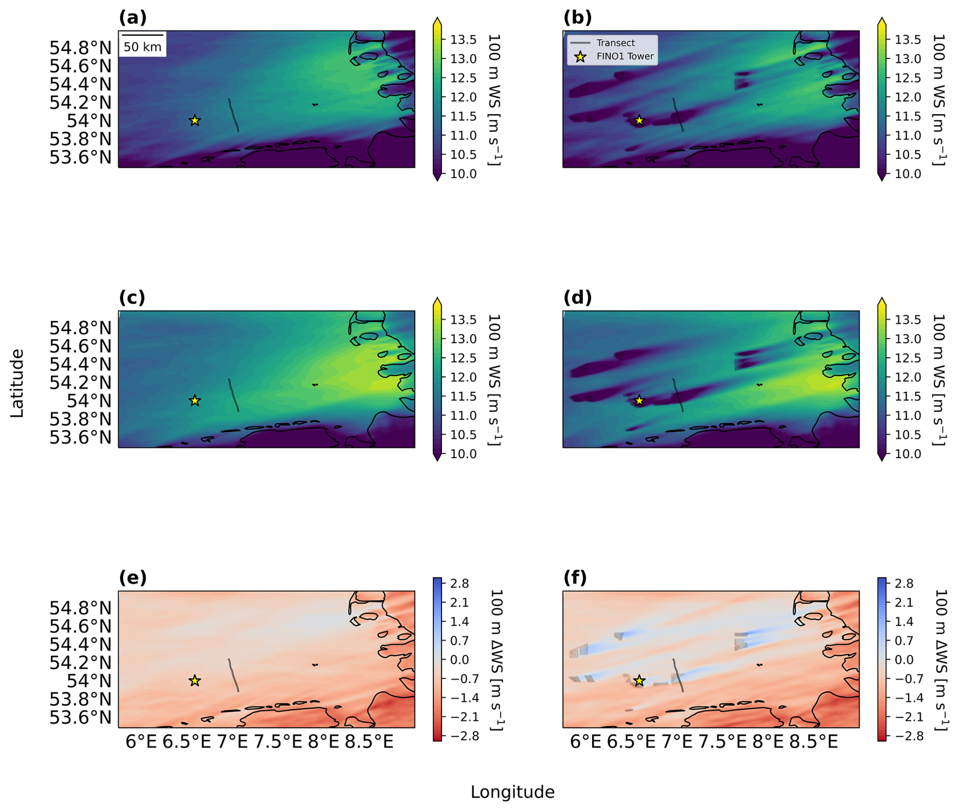
Figure A1 Horizontal wind speeds for the inner 1.67 km domain. (a) 3na_NA. (b) 3fa_025. (c) mna_NA. (d) mfa_025. (e) 3na_NA - mna_NA. (f) 3fa_025 – mfa_025. Turbines are marked with black circles, the FINO1 tower is marked with a yellow star, and the first transect path is marked with a solid line.

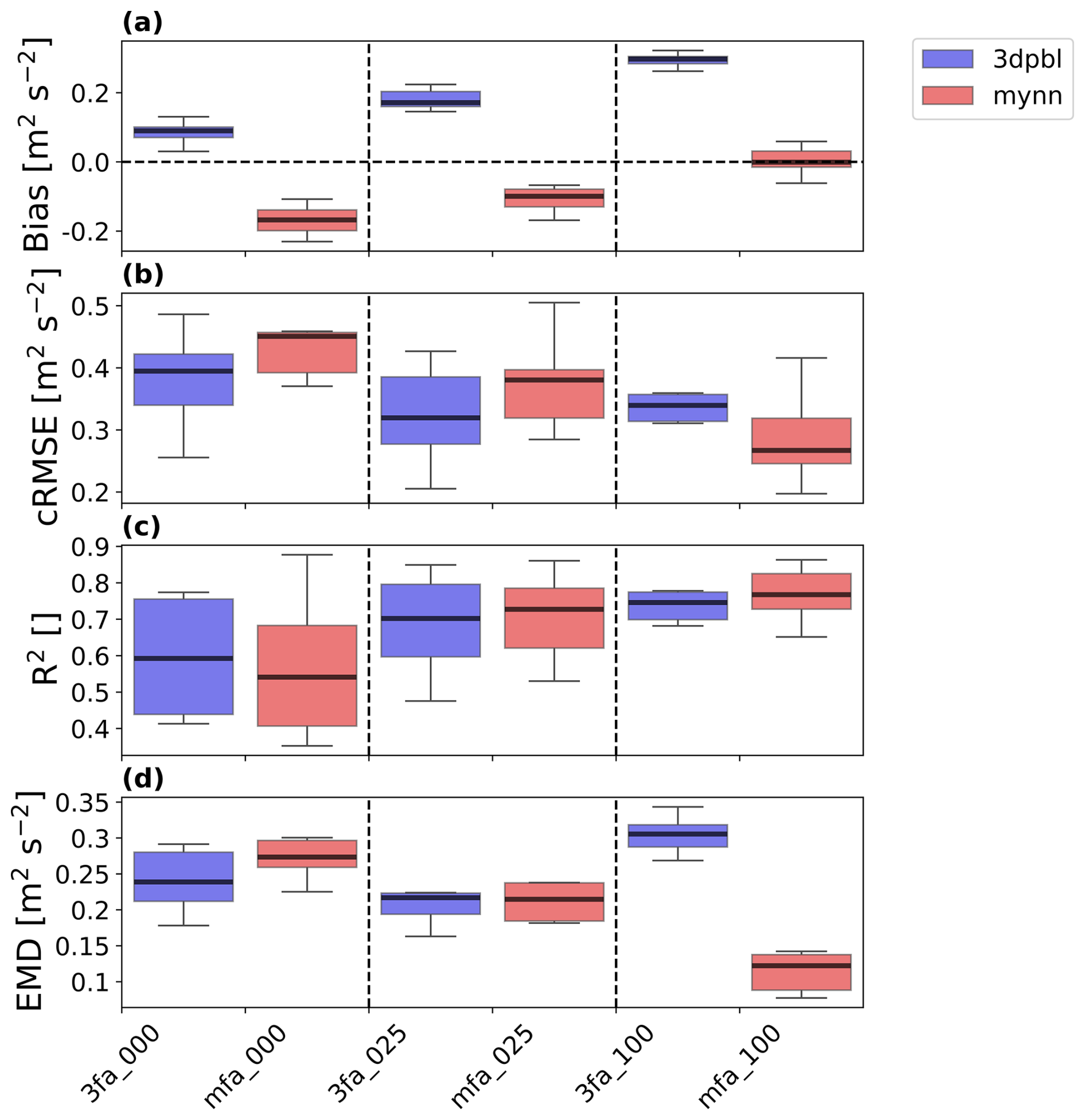
Figure A2 Error metric boxplot for aircraft observations collected at 250 m for TKE. The box and whiskers describe aircraft transect variability and are based on Q1 (25th percentile), Q3 (75th percentile), and the interquartile range (IQR) (Q3–Q1). The bar indicates the median. The box encloses the IQR, and the whiskers extend to $\mathrm{Q}\mathrm{1}-\mathrm{1.5}\times \mathrm{IQR}$ and $\mathrm{Q}\mathrm{3}+\mathrm{1.5}\times \mathrm{IQR}$. The simulation names are mapped according to the short names provided in Table 6, and the vertical dotted lines visually separate simulations by wind farm TKE factor. (a) TKE bias, (b) TKE cRMSE, (c) TKE R², (d) TKE EMD.

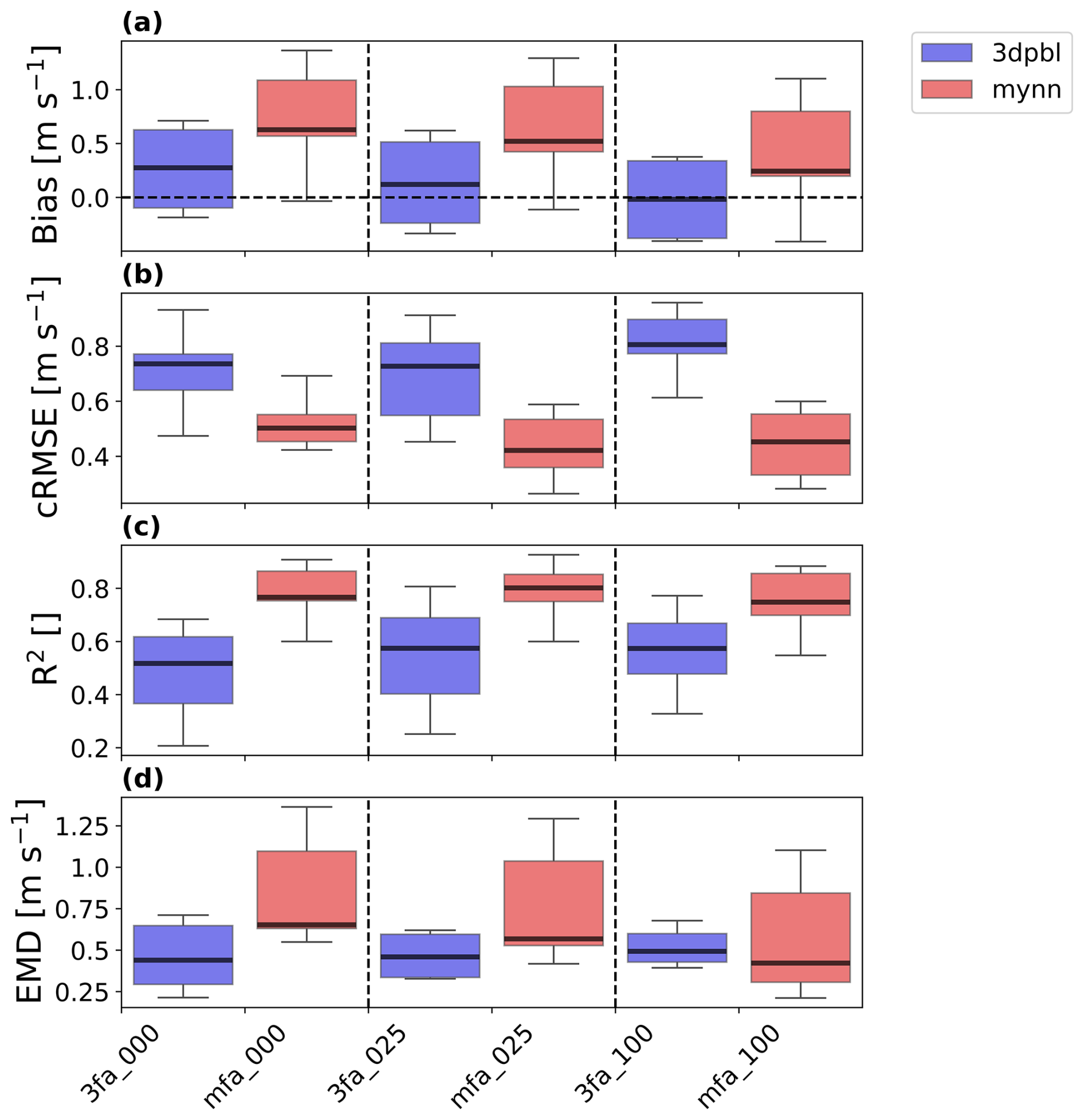
Figure A3 Error metric boxplot for aircraft observations collected at 250 m for wind speed. The box and whiskers describe aircraft transect variability and are based on Q1 (25th percentile), Q3 (75th percentile), and the interquartile range (IQR) (Q3–Q1). The box encloses the IQR, and the whiskers extend to $\mathrm{Q}\mathrm{1}-\mathrm{1.5}\times \mathrm{IQR}$ and $\mathrm{Q}\mathrm{3}+\mathrm{1.5}\times \mathrm{IQR}$. The simulation names are mapped according to the short names provided in Table 6, and the vertical dotted lines visually separate simulations by wind farm TKE factor. (a) Wind speed bias, (b) wind speed cRMSE, (c) wind speed R², (d) wind speed EMD.

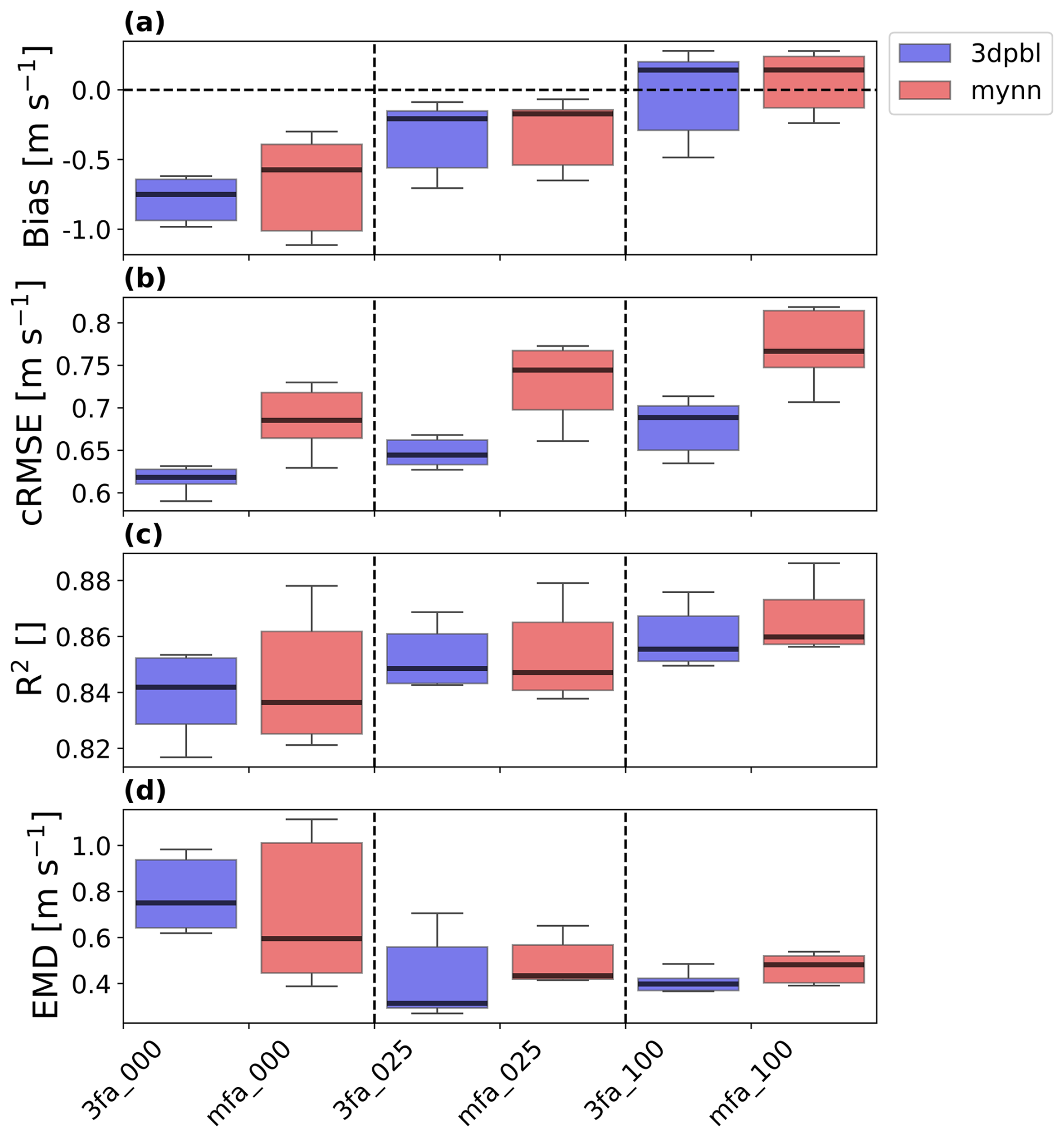
Figure A4 Error metric boxplot for the FINO1 tower measurements for wind speed. The box and whiskers describe FINO1 model height variability and are based on Q1 (25th percentile), Q3 (75th percentile), and the interquartile range (IQR) (Q3–Q1). The bar indicates the median. The box encloses the IQR, and the whiskers extend to $\mathrm{Q}\mathrm{1}-\mathrm{1.5}\times \mathrm{IQR}$ and $\mathrm{Q}\mathrm{3}+\mathrm{1.5}\times \mathrm{IQR}$. The simulation names are mapped according to the short names provided in Table 6, and the vertical dotted lines visually separate simulations by wind farm TKE factor. (a) Wind speed bias, (b) wind speed cRMSE, (c) wind speed R², (d) wind speed EMD.

A3 Effect of TKE advection

The appropriate treatment of the TKE advection option for simulations of wind farm impacts – and, specifically, this case study – has also received much discussion in the literature. Most recently, Ali et al. (2023) argued that the advection option should be turned off. Ali et al. (2023) make this judgment based on the Siedersleben et al. (2020) finding that performance in the aircraft region improved by turning the advection option off. However, Siedersleben et al. (2020) performed their analysis with a version of the Fitch scheme that included the advection bug. As such, the results presented in Siedersleben et al. (2020) are qualitatively different from those presented in Larsén and Fischereit (2021). Although Larsén and Fischereit (2021) performed their analysis after the advection bug was addressed and performed simulations with advection both on and off, Larsén and Fischereit (2021) argue that further analysis would be necessary to make a formal recommendation.

We recommend using TKE advection for this case study, in contrast to prior recommendations. We argue that the advection option should be included on two bases. First, we note that TKE advection was omitted only from early versions of MYNN for reasons of numerical stability and not on a physical basis (Olson et al., 2019). Second, we note the guidance from Wadler et al. (2023), who show that introducing TKE advection allows for a more realistic distribution of TKE and argue that TKE advection should be modeled in a closure scheme unless there is an explicit reason to exclude this process. In addition to this physical argument, we quantify the (statistically insignificant) performance differences depending on the advection option below.

Responses to the advection option may reflect locational differences. The results at the FINO1 location show greater sensitivity to the advection option than those at the aircraft measurement site. First, the FINO1 site is marked by a single grid cell at a wind farm's edge (Fig. 2a) and is surrounded by other cells with wind turbines. Slight horizontal adjustment of this FINO1 tower location would capture the local TKE source as opposed to the sink (Fig. A5c, d). In addition, because the FINO1 performance is defined by a single grid cell, local TKE imbalances between grid cells are not compensated for in averaging calculations. In contrast, the aircraft measurements experience several competing interfarm advection pools that are compensated for across a broader domain (Fig. A5a, b). The two sites are also at different measurement heights. As explored earlier, the FINO1 site more directly interacts with the turbine-induced turbulence at the rotor level than the aircraft region site does (Fig. 6). As such, the FINO1 site is more sensitive to TKE differences. Although introducing advection does support some vertical transport of TKE at the aircraft measurement locations (Fig. A6a, b), maximum TKE is still better aligned physically with the measurement altitude for the FINO1 observations (Fig. A6c, d). As a consequence, the FINO1 region measurements show greater sensitivity to the advection option than the aircraft region measurements.

Differences in the amount of TKE generated by the PBL scheme may also explain responses in the advection option. Local TKE imbalances are stronger for 3DPBL TKE (Fig. A5a, c and Fig. A6a, c) than for MYNN TKE (Figs. A6b, d and A6b, d). Because the 3DPBL scheme has larger TKE (Fig. 8b), the 3DPBL scheme is more sensitive to TKE movement throughout the region.

Note that all performance differences based on the advection option are statistically insignificant (Table A1). This statistical insignificance is maintained for all evaluated fields, error metrics, and sites. Thus, even when considering TKE characterization for the single-celled FINO1 site, the effects on performance for this analysis are negligible.

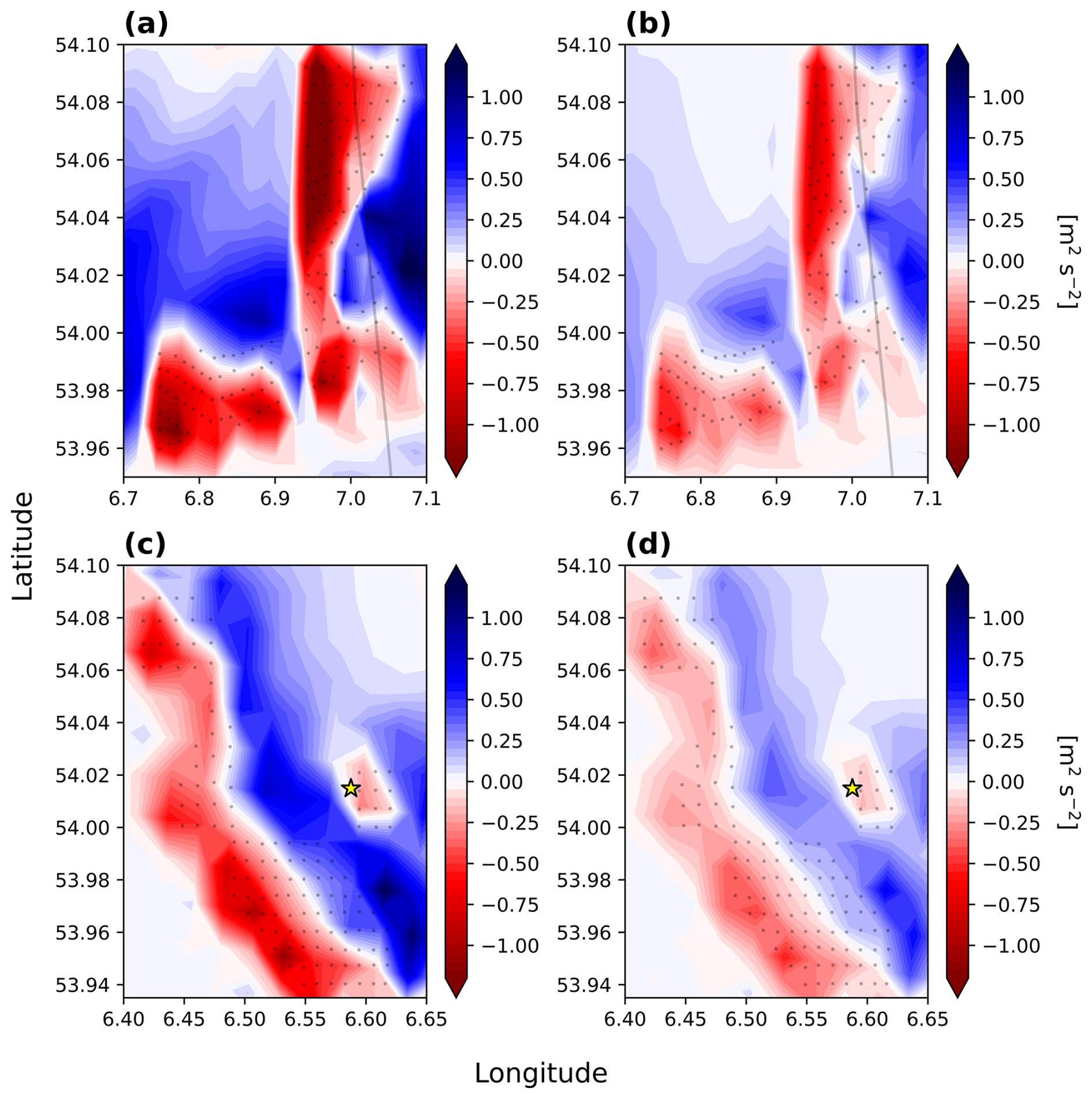
Figure A5 Horizontal slices to mark TKE differences between cases with advection on and cases with advection off. Red indicates that TKE is higher without advection. (a) Aircraft region 3fX_025. (b) Aircraft region mfX_025. (c) FINO1 3fX_025. (d) FINO1 3fX_025. FINO1 cases are averaged over the hours of 12:00:00–00:00:00, and the aircraft region cases are averaged over 14:10:00–16:10:00 UTC. Turbines are marked with black circles, the FINO1 tower is marked with a yellow star, and the first transect path is marked with a solid line.

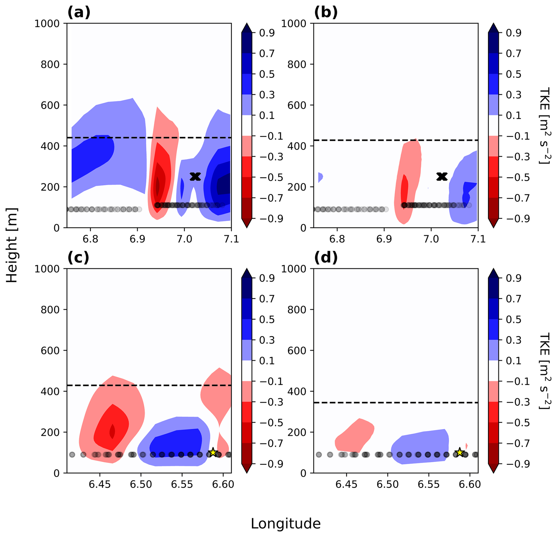
Figure A6 Vertical slices at a constant latitude of 54.03 to mark TKE differences between cases with advection on and cases with advection off. Red indicates that TKE is higher without advection. (a) Aircraft region 3fX_025. (b) Aircraft region mfX_025. (c) FINO1 3fX_025. (d) FINO1 3fX_025. FINO1 cases are averaged over the hours of 12:00:00–00:00:00, and the aircraft region cases are averaged over 14:10:00–16:10:00 UTC. Turbines are marked with black circles, the FINO1 tower is marked with a yellow star, and the first transect path is marked with a solid line.

Table A1 p values according to the Mann–Whitney U test. A bold cell indicates statistical significance at $\left|p\right|<=\mathrm{0.05}$. Only Fitch simulations with a wind farm TKE factor of 0.25 were considered.

A4 Effect of duration

Here, we provide an extended comparison of the performance of the two PBL schemes by comparison to observations at the FINO1 site. This evaluation was designed to reflect the FINO1 evaluation performed in the main text as closely as possible. As such, wind speed data were analyzed at the same seven (34, 41, 51, 61, 81, 91, 102 m) heights at the same 10 min temporal resolution considered in the main text. The evaluation was also performed with the same model cell with the same four error metrics (bias, cRMSE, R², and EMD) and Mann–Whitney U statistical significance testing. The evaluation period is the key difference between the main FINO1 evaluation and that performed here. The evaluation period (1 October–28 October) contains all the contiguous, numerically stable days in October 2017. Note that, to ensure this numerical stability, a time step of 18 s was selected instead of the 30 s time step employed in the main text.

The PBL schemes show mixed performance in the extended FINO1 evaluation. The 3DPBL scheme produces lower median cRMSE (Fig. A7b) and higher R² (Fig. A7c) than MYNN, whereas MYNN produces lower bias (Fig. A7a) and lower EMD (Fig. A7d) than 3DPBL. However, only the differences in cRMSE (Fig. A7b), bias (Fig. A7a), and R² (Fig. A7c) are statistically significant; the EMD (Fig. A7d) difference is not. Considering only statistically significant error metrics, 3DPBL performs better for two of the three metrics.

The longer time period also clarifies model differences. In both cases, 3DPBL shows the optimal cRMSE. However, in the 12 h analysis, statistically significant differences only emerged for cRMSE (Fig. 14d), whereas the 28 d analysis instead suggests statistically significant differences with respect to three error metrics (Fig. A7). Ultimately, the 28 d analysis corroborates the 12 h analysis by more fully confirming 3DPBL as the optimal scheme for this location with respect to more error metrics.

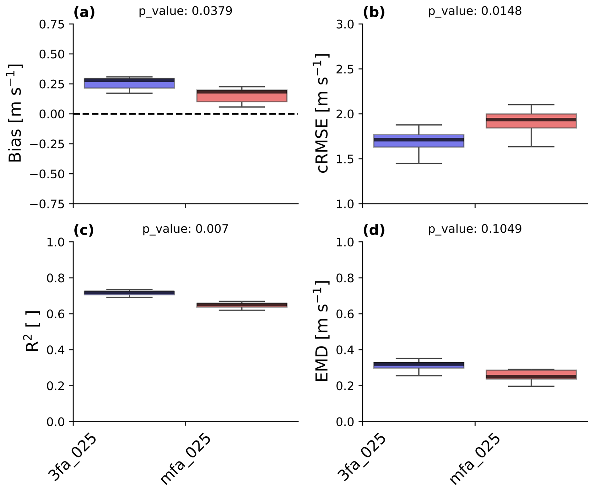
Figure A7 Error metrics across all Fitch simulations with the advection option on and with a wind farm TKE factor of 0.25 at the FINO1 site for the period of 1–28 October for wind speed. The bar shows the median. The box encloses the interquartile range (IQR), and the whiskers extend to $\mathrm{Q}\mathrm{1}-\mathrm{1.5}\times \mathrm{IQR}$ and $\mathrm{Q}\mathrm{3}+\mathrm{1.5}\times \mathrm{IQR}$. (a) Wind speed bias, (b) wind speed cRMSE, (c) wind speed R², (d) wind speed EMD.