Idealized simulations of wind farm interactions with intermittent turbulence in stable boundary layer conditions

Stable atmospheric boundary layer conditions typically correspond to weak turbulence levels, but intermittent periods of elevated turbulence can occur during otherwise quiescent conditions. The interaction between intermittent turbulence and wind turbines is not well understood because of sparse observations, as well as the difficulty in realistically resolving small-scale turbulence during strongly stable conditions with numerical simulations. In this study, an explicit filtering and reconstruction approach for large-eddy simulation (LES) is used to simulate weakly and strongly stable conditions, with surface cooling rates of −0.2 and −2.0 K h⁻¹, respectively. This approach can sustain resolved background turbulence at relatively coarse grid spacing and stronger stratification compared to conventional closures, permitting more realistic intermittent stable boundary layer (SBL) turbulence. The idealized LES capability of the Weather Research and Forecasting model is employed with turbine rotors parameterized using generalized actuator disks to examine (1) how the presence of turbine wakes affects SBL evolution and (2) the effect of intermittent turbulence on power production and wake recovery. Wakes increase mixing and deepen the SBL, with a stronger effect under strongly stable conditions, primarily because the SBL is shallower and closer to the top of the wind turbine rotor layer. Intermittent turbulence does not have a significant impact on mean power generation and wake recovery because the relevant intermittent turbulent structures in this study only affect the bottom half of the rotor disk. Power production is, however, more variable during periods of elevated turbulence, demonstrating the impact of SBL intermittency. This study uses an idealized configuration, focusing on LES model performance and physical understanding, with the goal of informing future simulations of the conditions observed during the American Wake Experiment.

1 Introduction

Onshore wind turbines experience the stable atmospheric boundary layer nearly every night. Stably stratified flows occur as the earth's surface cools in the absence of radiation from the sun. The associated buoyancy suppression results in small-scale and sometimes intermittent turbulence, which can be difficult to capture in numerical models. This relatively small-scale and low-amplitude ambient turbulence, especially when compared to daytime convective conditions, results in wind turbine and farm wakes sometimes persisting over 30 rotor diameters (30D) downwind (Hirth and Schroeder, 2013); this can exceed 4 km, depending on the turbine size. Additionally, turbine fatigue damage is highly correlated with strong vertical wind shear, periods of elevated turbulence, and wave-like motions, all of which are common in the stable boundary layer (SBL) (Sisterson and Frenzen, 1978; Mahrt, 2014). Representation of stably stratified turbulence is therefore critical when modeling wind farms to characterize and predict performance and power generation for the electrical grid.

Wind turbine performance during nocturnal stable conditions is highly dependent on many factors, including the strength of stability (e.g., Wharton and Lundquist, 2012; Vanderwende and Lundquist, 2012; Dimitrov et al., 2018, and Sanchez Gomez and Lundquist, 2020), as well as the presence of waves (e.g., Draxl et al., 2021; Lanzilao and Meyers, 2024, and Wise et al., 2025) and (possibly) turbulence intermittency. Low-level jets (LLJs), which occur frequently during stable conditions, can increase turbulence intensity and intermittency, as well as mean shear and veer profiles. For weak stability, shear production overcomes buoyancy, and turbulence is continuous in the SBL. However, for strong stability, turbulence can be suppressed or become intermittent.

The definition of “intermittent turbulence” varies in the published literature owing to its applicability to a range of SBL phenomena. Perhaps most simply, Mahrt (2014) defines intermittency as “strong variability of the turbulence in space and time.” Many observed SBL phenomena can be described as intermittent. More technically, turbulence intermittency in the atmosphere has been broken down into two main categories (Mahrt, 1989, 1999). Mahrt (1989) defines small-scale intermittency as a substructure of the main coherent eddies in a flow and global intermittency as the patchiness of turbulence on scales larger than the main eddies. Global intermittency can be broken down further into two types: external and internal. External intermittency is caused by nonstationary submesoscale motions, whereas internal intermittency is caused by shear instability (Mahrt, 2014). Examples of nonstationary submesoscale motions that trigger external intermittency include breaking gravity waves, bores, Kelvin–Helmholtz billows, terrain-induced flows, and propagating density currents (Rottman and Simpson, 1989; Sun et al., 2002; Banta, 2008; Mahrt, 2014). Conversely, for internal intermittency, shear increases locally within the stable boundary layer (not only at the surface), inducing instability and mixing (Mahrt, 2014; Sun et al., 2015). Internal intermittency can be a cyclic process as mixing leads to decreased shear and turbulence decay, but as shear eventually builds back up, instability occurs again. This process tends to occur during strongly stable conditions due to the high shear requirement. It is sometimes referred to as the upside-down SBL because the most energetic turbulence is generated by shear aloft rather than by shear in the near-surface region (Mahrt, 1985, 1999; Sun et al., 2002; Banta, 2008).

Internal intermittency is the main focus of this study and is quantified following Coulter and Doran (2002), who used turbulent heat fluxes from sonic anemometer and meteorological tower data during the Cooperative Atmospheric Surface Exchange Study (CASES-99) to calculate an “intermittency fraction.” Here we extend their quantification method from turbulent heat flux to turbulence kinetic energy, which is the primary focus of our analysis and is a more common and accessible metric for assessing turbulence in the wind energy community. The intermittency fraction is based on the cumulative distribution of a turbulent quantity during an analysis period. A threshold is determined as the value at which 50 % of the cumulative distribution function is reached. Periods with the turbulent quantity greater than the threshold are considered active “bursts” or turbulent. On intermittent nights, Coulter and Doran (2002) found intermittency fractions between 15 % and 30 %, which for a 12 h nighttime period means that the majority of the turbulence occurs over a window of just 1.8–3.6 h.

There are a number of other methods to quantify intermittency available in the literature. For example, Holtslag and Nieuwstadt (1986) proposed a scaling condition based on the boundary layer depth, the altitude within the boundary layer, and the Obukhov length. However, this scaling condition is not designed to determine when flow is turbulent or quiescent in a time-dependent sense. In van der Linden et al. (2020), time periods are defined as turbulent when the horizontally averaged kinematic temperature flux at the top of the boundary layer in their simulations became greater than the surface temperature flux. In their study, they found an intermittency fraction of roughly 26 %, similar to those observed by Coulter and Doran (2002). Ultimately, we follow Coulter and Doran (2002) as their method is observation-based but can be easily applied to simulation datasets. For example, their method could be applied to the observational network at the American Wake Experiment (AWAKEN) in future analyses.

Intermittent turbulence in the SBL can affect turbine power production, wake recovery, and structural loading, each of which can impact the predictability and reliability of power reaching the grid. Among the goals of the recent AWAKEN field campaign is to investigate the role of intermittent turbulent bursting events on the aforementioned concerns (Moriarty et al., 2020). The AWAKEN field campaign serves as the inspiration for the present study, which focuses on idealized flow and flat terrain to better understand intermittent turbulence interactions with wind farms. We simulate weak- and strong-stability conditions to study the interaction between wind turbines and the SBL, with the goals of (1) determining how the presence of wind turbine wakes affects stable boundary layer evolution, and (2) examining the effect of intermittent turbulence on power production and wake recovery.

To answer these questions, we use large-eddy simulation (LES); however, there have been a number of LES studies that demonstrate the sensitivity of simulation results in SBL conditions on the turbulence closure scheme. Beare et al. (2006) found that at a moderate grid spacing (6.25 m), mean profiles were highly dependent on the turbulence closure; however, at fine resolutions of 2 m or less, there were only small changes in mean profiles. Zhou and Chow (2011) modeled a range of SBLs, comparing the common turbulence kinetic energy order-1.5 (TKE-1.5) closure (Deardorff, 1980) and the dynamic reconstruction model (DRM) (Chow et al., 2005) at various grid resolutions in idealized conditions. Unlike the TKE-1.5 closure, the DRM closure accounts for backscatter or the transfer of energy from the subfilter scale to resolved scales, which Zhou and Chow (2011) found to improve the representation of near-surface profiles under moderate and strong (∼2.0 K h⁻¹) stability conditions. As a result, the DRM closure was able to sustain resolved turbulence and better represent mean wind and potential temperature profiles at coarser resolutions ($\mathit{\{}\mathrm{\Delta }x,\mathrm{\Delta }z\mathit{\}}=\mathit{\{}\mathrm{8}\mathrm{m},\mathrm{2.5}\mathrm{m}\mathit{\}}$ and $\mathit{\{}\mathrm{\Delta }x,\mathrm{\Delta }z\mathit{\}}=\mathit{\{}\mathrm{16}\mathrm{m},\mathrm{5}\mathrm{m}\mathit{\}}$) compared to the TKE-1.5 closure, which needed grid spacing as fine as $\mathrm{\Delta }x=\mathrm{\Delta }z=\mathrm{3.125}$ m. The DRM closure was also used to simulate a real case of intermittent turbulence during the CASES-99 field campaign (Zhou and Chow, 2014). Zhou and Chow (2014) used a multi-scale nested setup with a horizontal grid spacing of 25 m on the finest (LES) domain. They found that intermittent turbulence could be generated through gravity wave breaking over a cold-air pool in a valley upwind of measurements. However, wave breaking only occurred in the simulations when using the DRM closure.

In this study, we use LES and the DRM turbulence closure to simulate weak and strong SBL conditions with a wind turbine parameterization (Sect. 2) to comprehensively explore a range of SBL interactions with a wind farm. This builds on a number of previous studies in the literature, which have used idealized LES to examine certain SBL conditions for modeling wind turbine and wind farm flows (Lu and Porté-Agel, 2011; Marjanovic et al., 2017; Gadde and Stevens, 2021b; Sanchez Gomez et al., 2023), as well as other studies that have proven the efficacy of the DRM closure for capturing intermittent turbulent events (Zhou and Chow, 2011, 2014; Wise et al., 2025). First, we analyze the effect of the turbulence closure on SBL development for both regimes (Sect. 3.1). Then, because the strongly stable regime is intermittently turbulent, we quantify intermittency (Sect. 3.2). Lastly, we analyze the interaction between the wind farm and different SBL conditions focusing on wind farm power production (Sects. 3.3 and 3.4), followed by conclusions and recommendations for future work (Sect. 4).

2 Methods

2.1 WRF-LES-GAD

To study wind farm performance in a range of SBL conditions, we use the LES capability of the WRF model (Skamarock et al., 2021), version 4.4, with a generalized actuator disk (GAD) wind turbine implementation (Mirocha et al., 2014b), hereinafter referred to as WRF-LES-GAD. The GAD model implemented in WRF follows blade element momentum theory and requires specifications for the turbine's airfoil lift and drag coefficients. These coefficients come from a 1.6 MW wind turbine parameterization used in Arthur et al. (2020), which has an 80 m hub height and 80 m rotor diameter (D). This GAD implementation typically requires a grid spacing of at least 10 m to capture the effect of the rotor drag on the resolved flow (Mirocha et al., 2014b, 2015; Arthur et al., 2020; Wise et al., 2022; Sanchez Gomez et al., 2022, 2023).

Our WRF-LES-GAD build also includes a modified surface layer implementation (Mirocha et al., 2015), which iteratively solves for velocities and temperature at the first grid point above the surface using Monin–Obukhov similarity theory (MOST) (Monin and Obukhov, 1954). WRF's native MOST implementation only allows a surface heat flux condition to be specified; the modified surface layer scheme allows a cooling rate to be specified and calculates the surface heat flux and friction velocity based on universal functions for MOST (Businger et al., 1971). MOST is based on the assumption of continuous turbulence; however, as stability increases (and turbulence becomes intermittent), the applicability of MOST decreases (Chenge and Brutsaert, 2005; Kumar and Sharan, 2012). Nevertheless, in the absence of widely accepted alternatives for representing the surface layer and bottom boundary condition, we continue with MOST and seek to extend the model to very stable stratification.

LES includes a spatial filter which separates the larger resolved scales from the subfilter-scale (SFS) motions. This filter can be implicit – based on the grid scale – or explicit. The effects of the SFS scales on the resolved scales are then parameterized using a turbulence model. As stability increases, the energetic turbulent motions become smaller and smaller, requiring a finer grid to resolve them (Wyngaard, 2010). The most common LES schemes use an eddy-viscosity model with no explicit filter to relate SFS and resolved motions. These models are entirely dissipative with energy transfer from larger scales to smaller scales (Wyngaard, 2004); however, energy transfer from small to large scales can be important, especially in stably stratified environments (Sullivan et al., 2003). More sophisticated turbulence closures are able to account for this backscatter of energy using an explicit filtering approach. Here, we use the dynamic reconstruction model (DRM) of Chow et al. (2005) to extend the working range of LES and to analyze turbine–airflow interactions in more stably stratified flows. Comparisons are also made to the commonly used turbulent kinetic energy order-1.5 model (TKE-1.5) (Deardorff, 1980), which solves a prognostic TKE equation with a grid-based length scale to define the eddy viscosity.

2.2 Dynamic reconstruction turbulence model

The dynamic reconstruction model uses a 3D (top-hat) filter applied to the Navier–Stokes equations to separate large and small scales. This filter is twice the grid cell spacing and is applied explicitly in the model; it is thus distinct from the implicit effects of grid discretization. The effect of the implicit grid filter, as well as numerical truncation errors, is to prohibit motions smaller than the grid scale. There is thus a range of scales between the grid scale and the filter scale that can be partially reconstructed in the model using an inverse filtering operation (Chow et al., 2005).

The governing explicitly filtered Navier–Stokes equations of LES on a discrete grid are

$$\begin{array}{}\text{(1)}& {\displaystyle }{\displaystyle \frac{\partial {\stackrel{\mathrm{‾}}{\stackrel{\mathrm{̃}}{u}}}_i}{\partial t}}+{\displaystyle \frac{\partial \stackrel{\mathrm{̃}}{{\stackrel{\mathrm{‾}}{\stackrel{\mathrm{̃}}{u}}}_j{\stackrel{\mathrm{‾}}{\stackrel{\mathrm{̃}}{u}}}_i}}{\partial x_j}}=-{\displaystyle \frac{\mathrm{1}}{\mathit{\rho }}}{\displaystyle \frac{\partial \stackrel{\mathrm{‾}}{\stackrel{\mathrm{̃}}{p}}}{\partial x_i}}+\mathit{\nu }{\displaystyle \frac{{\partial }^{\mathrm{2}}{\stackrel{\mathrm{‾}}{\stackrel{\mathrm{̃}}{u}}}_i}{\partial x_i\partial x_j}}-{\displaystyle \frac{\partial {\stackrel{\mathrm{̃}}{\mathit{\tau }}}_{ij}}{\partial x_j}}+F_i,\end{array}$$

where x_i represents the x, y, and z spatial dimensions; u_i are velocities; p is pressure; ρ is density; τ is the turbulent stress; and ${\stackrel{\mathrm{̃}}{F}}_i$ represents a body force (such as drag from a wind turbine rotor). The overbar operator represents explicit filtering via a smooth spatial filter, and the tilde operator is representation of the implicit filter operation. The operators combined represent a resolved and filtered field; thus ${\stackrel{\mathrm{‾}}{\stackrel{\mathrm{̃}}{u}}}_i$ is the resolved, explicitly filtered velocity. See Gullbrand and Chow (2003) and Chow et al. (2005) for more details on the notation.

The full turbulent stress term is referred to as the subfilter-scale stress (τ^SFS), which is made up of two components: a resolvable subfilter-stress (RSFS), τ^RSFS, and a subgrid-scale (SGS) stress, τ^SGS.

$$\begin{array}{ll}{\displaystyle }{\mathit{\tau }}^{\text{SFS}}& {\displaystyle }={\mathit{\tau }}_{ij}={\mathit{\tau }}^{\text{SGS}}+{\mathit{\tau }}^{\text{RSFS}}\\ \text{(2)}& {\displaystyle }& {\displaystyle }=\left(\stackrel{\mathrm{‾}}{u_i{u}_j}-\stackrel{\mathrm{‾}}{{\stackrel{\mathrm{̃}}{u}}_i{\stackrel{\mathrm{̃}}{u}}_j}\right)+\left(\stackrel{\mathrm{‾}}{{\stackrel{\mathrm{̃}}{u}}_i{\stackrel{\mathrm{̃}}{u}}_j}-{\stackrel{\mathrm{‾}}{\stackrel{\mathrm{̃}}{u}}}_i{\stackrel{\mathrm{‾}}{\stackrel{\mathrm{̃}}{u}}}_j\right)\end{array}$$

The RSFS term represents the range of eddy motions between the implicitly defined grid filter (i.e., the Nyquist limit) and the explicit LES filter. When an explicit filter is defined, τ^RSFS is resolvable on the grid, but this term is generally ignored in conventional turbulence closures which only parameterize SGS stresses.

For the DRM closure, the subgrid-scale stress, τ^SGS, is parameterized using the dynamic Wong–Lilly (DWL) (Wong and Lilly, 1994) eddy-viscosity model:

$$\begin{array}{}\text{(3)}& {\displaystyle }{\displaystyle }{\mathit{\tau }}^{\text{SGS}}=-\mathrm{2}{\mathit{\nu }}_t{\stackrel{\mathrm{‾}}{\stackrel{\mathrm{̃}}{S}}}_{ij},\end{array}$$

where ${\stackrel{\mathrm{‾}}{\stackrel{\mathrm{̃}}{S}}}_{ij}$ is the filtered and resolved strain rate tensor, and ${\mathit{\nu }}_t=C_{\mathit{ϵ}}{\mathrm{\Delta }}^{\mathrm{4}/\mathrm{3}}$ is the dynamic eddy viscosity. Here, Δ is the filter width, and $C_{\mathit{ϵ}}{\mathrm{\Delta }}^{\mathrm{4}/\mathrm{3}}$ is determined dynamically using the least-squares method of Lilly (1992).

The RSFS stress is determined by reconstructing the velocity field using the approximate deconvolution method (Stolz et al., 2001):

$$\begin{array}{}\text{(4)}& {\displaystyle }{\displaystyle }{\stackrel{\mathrm{̃}}{u}}_i\approx {\stackrel{\mathrm{‾}}{\stackrel{\mathrm{̃}}{u}}}_i+(I-G)*{\stackrel{\mathrm{‾}}{\stackrel{\mathrm{̃}}{u}}}_i+(I-G)*\left[(I-G)*{\stackrel{\mathrm{‾}}{\stackrel{\mathrm{̃}}{u}}}_i\right]+\mathrm{\dots },\end{array}$$

where I is the identity matrix, G is the explicit filter, and * represents the convolution operator. Each additional term in the series adds a level of reconstruction that more accurately represents the RSFS velocities. In this study, level-0 reconstruction is used, which includes the first term in the series, and the velocity is approximated as the filtered velocity. This level-0 reconstruction is the same as the scale-similarity model of Bardina (Bardina et al., 1983). Combined with the eddy-viscosity SGS term, this level-0 reconstruction becomes a dynamic mixed model (Zang et al., 1993). Higher levels of reconstruction have been the focus of other studies (Zhou and Chow, 2011; Simon et al., 2019), with increasing levels restoring turbulent scales near the filter cutoff (Zhou and Chow, 2011); however, we focus on level-0 reconstruction as it results in the biggest benefit with the least added computational cost. We refer to the closure as DRM for simplicity and to indicate the more general implementation in WRF.

Lastly, near-wall stresses are usually underpredicted with dynamic SGS models applied in atmospheric boundary layer (ABL) flows (Chow et al., 2005). A near-wall stress model (Brown et al., 2001) is used to account for this, which has improved agreement with similarity theory in previous studies (Chow et al., 2005; Zhou and Chow, 2011, 2012; Kirkil et al., 2012). The near-wall stress is defined for $i=\mathrm{1},\mathrm{2}$ and is added only to the τ_i3 terms, as follows:

$$\begin{array}{}\text{(5)}& {\displaystyle }{\displaystyle }{\mathit{\tau }}_{i\mathrm{3}}^{\text{near-wall}}\left(z\right)=-\int C_{c}a\left(z\right)\left|\stackrel{\mathrm{‾}}{\stackrel{\mathrm{̃}}{u}}\right|{\stackrel{\mathrm{‾}}{\stackrel{\mathrm{̃}}{u}}}_i\mathrm{d}z,\end{array}$$

where C_c is a strength factor, set to 0.5 due to the grid-aspect ratio in this study, and a(z) is a shape function set to smoothly decay the effect of the near-wall stress at a specific cutoff height H_c (Chow et al., 2005; Kirkil et al., 2012). H_c is chosen as 2Δx following Zhou and Chow (2011). The shape function is defined as

$$\begin{array}{}\text{(6)}& {\displaystyle }{\displaystyle }a\left(z\right)={\text{cos}}^{\mathrm{2}}\left({\displaystyle \frac{\mathit{\pi }z}{\mathrm{2}{H}_c}}\right).\end{array}$$

The DWL eddy-viscosity model and the scale-similar RSFS term are combined to create a mixed-model for turbulence. This mixed model along with the added near-wall stress result in

$$\begin{array}{ll}{\displaystyle }{\mathit{\tau }}_{ij}& {\displaystyle }={\mathit{\tau }}^{\text{RSFS}}+{\mathit{\tau }}^{\text{SGS}}\\ \text{(7)}& {\displaystyle }& {\displaystyle }=\stackrel{\mathrm{‾}}{{\stackrel{\mathrm{̃}}{u}}_i{\stackrel{\mathrm{̃}}{u}}_j}-\stackrel{\mathrm{‾}}{{\stackrel{\mathrm{̃}}{u}}_i}\stackrel{\mathrm{‾}}{{\stackrel{\mathrm{̃}}{u}}_j}-\mathrm{2}{C}_{\mathit{ϵ}}{\mathrm{\Delta }}^{\mathrm{4}/\mathrm{3}}{\stackrel{\mathrm{‾}}{\stackrel{\mathrm{̃}}{S}}}_{ij}+{\mathit{\tau }}_{i,\text{near-wall}}\end{array}$$

With the DRM's formulation for RSFS motions, subfilter-scale turbulent dissipation $\mathit{ϵ}=-{\mathit{\tau }}_{ij}{\stackrel{\mathrm{‾}}{\stackrel{\mathrm{̃}}{S}}}_{ij}$ can vary both positively and negatively, representing dissipation and backscatter. It is worth noting that in conventional closures, such as TKE-1.5, the eddy-viscosity form is purely dissipative (Wyngaard, 2004). This is because the SFS stress does not represent RSFS motions and only encompasses SGS motions, resulting in ϵ being strictly positive.

The SFS scalar fluxes in the DRM follow a similar procedure to momentum. The SFS fluxes are comprised of two terms: the SGS eddy-diffusivity contribution from the DWL model and the RSFS contribution from the approximate deconvolution method. The SFS potential temperature, θ, flux in the DRM model is

$$\begin{array}{}\text{(8)}& {\displaystyle }{\displaystyle }{\mathit{\tau }}_{\mathit{\theta }j}=\underset{{\mathit{\tau }}_{\mathit{\theta }j}^{\text{RSFS}}}{\underbrace{\stackrel{\mathrm{‾}}{\stackrel{\mathrm{̃}}{\mathit{\theta }}{\stackrel{\mathrm{̃}}{u}}_j}-\stackrel{\mathrm{‾}}{\stackrel{\mathrm{̃}}{\mathit{\theta }}}{\stackrel{\mathrm{‾}}{\stackrel{\mathrm{̃}}{u}}}_j}}\underset{{\mathit{\tau }}_{\mathit{\theta }j}^{\text{SGS}}}{\underbrace{-\mathrm{2}{\mathit{\nu }}_{t,h}{\displaystyle \frac{\partial \stackrel{\mathrm{‾}}{\stackrel{\mathrm{̃}}{\mathit{\theta }}}}{\partial x_j}}}},\end{array}$$

where ν_t,h is the dynamic, scalar eddy diffusivity defined as ${\mathit{\nu }}_{t,h}={\mathit{\nu }}_t/\mathit{\text{Pr}}$, with $\mathit{\text{Pr}}=\mathrm{1}/\mathrm{3}$ as defined in WRF (Skamarock et al., 2021).

2.3 Turbulent kinetic energy 1.5-order model

The TKE-1.5 model (Deardorff, 1980) is an eddy-viscosity turbulence closure which solves a prognostic turbulent kinetic energy (TKE) equation to obtain a characteristic turbulent velocity scale and uses the grid spacing as the length scale to parameterize the SGS stresses (Deardorff, 1980; Moeng, 1984; Moeng and Sullivan, 1994). The TKE equation describes the evolution of TKE and parameterizes sources and sinks from shear production, buoyancy production or suppression, turbulent mixing, and dissipation (Deardorff, 1980; Moeng, 1984; Skamarock et al., 2021). The eddy viscosity is defined as

$$\begin{array}{}\text{(9)}& {\displaystyle }{\displaystyle }{\mathit{\nu }}_t=C_k{l}_{h,v}{\mathrm{e}}^{\mathrm{1}/\mathrm{2}},\end{array}$$

where e is the TKE, and C_k is a constant (set to 0.15). The length scales are defined anisotropically, with the horizontal length scale defined as $l_h=(\mathrm{\Delta }x\mathrm{\Delta }y{)}^{\mathrm{1}/\mathrm{2}}$, with Δx,Δy representing the grid spacing in the corresponding direction. The vertical length scale depends on the Brunt–Väisälä frequency, N, and is given by

$$\begin{array}{}\text{(10)}& {\displaystyle }{\displaystyle }{l}_v=\left\{\begin{array}{ll}min\left[\mathrm{\Delta }z,\mathrm{0.76}\frac{{\mathrm{e}}^{\mathrm{1}/\mathrm{2}}}{N}\right]& :N^{\mathrm{2}}>\mathrm{0}\\ \mathrm{\Delta }z& :N^{\mathrm{2}}\le \mathrm{0}\end{array}\right..\end{array}$$

The scalar eddy diffusivity is defined for TKE-1.5 in the same way as the SGS component of the DRM model above:

$$\begin{array}{}\text{(11)}& {\displaystyle }{\displaystyle }{\mathit{\tau }}_{\mathit{\theta }j}=-\mathrm{2}{\mathit{\nu }}_{t,h}{\displaystyle \frac{\partial \stackrel{\mathrm{‾}}{\stackrel{\mathrm{̃}}{\mathit{\theta }}}}{\partial x_j}}.\end{array}$$

2.4 Simulation setup

WRF-LES-GAD is run in idealized mode, with a one-way nested and flat terrain setup to study how a range of SBL conditions interact with a wind farm. The wind farm's inflow conditions are based on the outer domain, which is periodic and unaffected by the turbine wakes (due to one-way nesting, wakes are confined to the inner domain). The outer domain size is $(Nx,Ny,Nz)=(\mathrm{750},\mathrm{500},\mathrm{120})$, which at a horizontal grid spacing of 8 m results in a physical domain size $\mathrm{6.0}\mathrm{km}\times \mathrm{4.0}\mathrm{km}\times \mathrm{1.0}\mathrm{km}$ ($x\times y\times z$). The inner domain has the same resolution as the outer domain but has two fewer grid points in x and y to ensure that the inner domain fits within the outer domain. The outer domain with periodic boundary conditions is spun up for 12 h, then the inner domain with a 3×3 array of wind turbines (see Fig. 1) is nested within the outer domain. The combined nested domains are then run for 2 h. The total simulation time is 14 h for the outer domain and 2 h for the inner domain, with all analysis completed from hour 13–14. This is a computationally efficient approach which allows for turbulence to develop and for the fluxes to become quasi-steady on the periodic outer domain while also accounting for a 1 h spin-up period of the turbine wakes on the inner domain. This minimal nesting setup has been previously used by Sanchez Gomez et al. (2023) to allow for the study of blockage in front of a wind farm in the inner domain using turbulence developed from an outer domain with periodic boundary conditions.

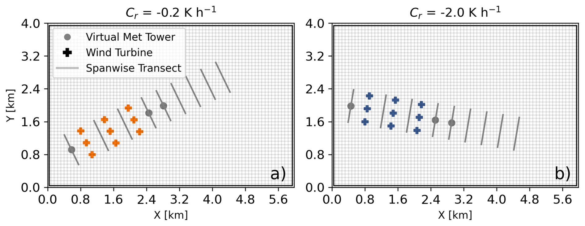
Figure 1 Simulation setup for the (a) weakly and (b) strongly stable regimes denoted by the surface cooling rate C_r. The virtual meteorological tower is located 5D upwind of the wind farm, and the lines represent 10D-wide transects at various locations upwind, within, and downwind of the wind farm.

Distinct wind farm configurations are used for two different cooling rates to account for changes in wind direction at hub height. As discussed below, the wind direction varies significantly with height (wind veer) in the stable boundary layer and therefore produces very different wind directions at hub height for different stability conditions, even with the same geostrophic forcing. The 3×3 wind farm is therefore aligned with the hub-height wind direction (known a priori from the outer grid spinup) for each test case, as shown in Fig. 1, to maximize efficiency in the computational domain. The turbines are spaced 320 m or 4D in the spanwise direction and 8D in the streamwise direction. For the weakly stable configuration, the edge of each wind farm is located 800 m from the western and southern boundaries; i.e., the closest any turbine gets to a boundary is 800 m. For the strongly stable configuration, the closest turbine to the western boundary is also 800 m; however, the distance between the closest turbine and the southern boundary is increased from 800 to 1200 m to account for the extreme wind veer. Figure 1 also shows points 5D upwind of the first row of turbines, as well as 5D and 10D downwind of the third row of turbines, where u, v, w, and T are output at all vertical levels at the model time step meant to represent a virtual meteorological tower or vertical profiling lidar. Spanwise transects 10D or 800 m wide are also shown in Fig. 1 at various locations, which are used for analysis later in this work.

The simulations are forced with a geostrophic wind speed of U_G=10 m s⁻¹, V_G=0 m s⁻¹, which is typical in idealized studies (Kirkil et al., 2012; Zhou and Chow, 2011; Jiménez and Cuxart, 2005; Mirocha et al., 2014a). The two surface cooling rates used are −0.2 and −2.0 K h⁻¹ to represent weakly and strongly stable conditions. These cooling rates fall within the range used by Zhou and Chow (2011), who modeled weakly to strongly stable conditions. The grid has 8 m horizontal spacing and a vertical spacing of 2.5 m near the surface, with a gradual increase in spacing with height. These spacings are chosen because previous research has shown that the DRM is able to sustain resolved turbulence on this grid (Zhou and Chow, 2011). The 8 m grid spacing is also close to the moderate, 6.25 m spacing used in the SBL LES studies by Beare et al. (2006), which was shown to provide reasonable accuracy but with high dependence on the turbulence closure.

At the bottom boundary, surface cooling is prescribed using Monin–Obukhov similarity theory. The surface fluxes are determined using the constants and relationships from Businger et al. (1971), and the surface roughness, z₀, is set to 0.1 m. This surface roughness is appropriate for low crops with occasional large obstacles, which is characteristic of the AWAKEN site, especially during the summer season (Krishnamurthy et al., 2021). This configuration of the bottom boundary directly follows the methods of Zhou and Chow (2012). The potential temperature profile used for initialization is neutral at 300 K for the first 100 m, with stable stratification of 4 K km⁻¹ prescribed above. The initial profile is not meant to represent observed meteorological conditions but instead follows common practice in idealized SBL LES studies (Beare et al., 2006; Zhou and Chow, 2011; Peña et al., 2021; Gadde and Stevens, 2021a, b) where relatively shallow initial boundary layer depths and prescribed inversion strengths are used to control the development of the stable boundary layer. In our configuration, the imposed inversion strength and initial inversion height together promote the formation of an LLJ and turbulent entrainment at the capping inversion. As the simulation evolves, turbulence-driven entrainment increases the ABL depth and provides a significant pathway for downward transport of momentum and heat from the free atmosphere into ABL, contributing to wind turbine wake recovery (van der Laan and Sørensen, 2017) as discussed later.

When examining the effect of the turbulence closure model, only the outer domain is analyzed (i.e., wind turbine effects are not included). Additional runs at a horizontal grid spacing of 4 m are performed for both the DRM and TKE-1.5 closures as a reference (see Appendix A). Since turbulence in LES is strongly tied to the grid spacing, this sensitivity study allows us to assess model quality for both grid spacings and turbulence schemes.

3 Results and discussion

3.1 Effect of turbulence closure

For both regimes, as expected, a LLJ develops at the top of the SBL. Planar- and time-averaged vertical profiles of wind speed, wind direction, and potential temperature are shown in Fig. 2 for the 8 m grid spacing setup. All simulations are run for 14 h, and outputs are set to every 30 s during the analysis period from hour 13–14, resulting in 120 time instances in the time average. The simulations using 4 m resolution are very similar but with minor differences in the height of the LLJ (not shown). While 13 h of surface cooling is not necessarily realistic, selecting an analysis window after this many hours is commonly done in idealized SBL studies (Beare et al., 2006; Gadde and Stevens, 2021a, b; Peña et al., 2021). Additionally, turbulence statistics were found to be quasi-steady for the weakly stable regime (not shown). The fluxes do not reach a quasi-steady state for the strongly stable regime due to intermittency; therefore, we select hour 13–14 for consistency. When the surface is cooled, in LES, it takes many hours until the Coriolis forcing and surface friction balance with super-geostrophic flow at the top of the stable layer. This super-geostrophic flow represents a LLJ (see Fig. 2) and is a phenomenon commonly observed onshore at night (Vanderwende et al., 2015).

The effect of the different cooling rates is clearly observed in the differing LLJ heights in Fig. 2a. The wind speed profiles are very strongly sheared and become super-geostrophic at the top of the SBL. The maximum wind speed within the LLJ is close to 12 m s⁻¹ for both cases, with this maximum occurring at 290 m for the weakly stable regime and 70 m for the strongly stable regime. While the wind speed at the nose of the LLJ is similar in both cases, the 80 m hub-height wind speed varies greatly due to the shear. The hub-height wind speed is 7.5 m s⁻¹ for the weakly stable regime and 12.0 m s⁻¹ for the strongly stable regime. The wide range of wind speeds across the rotor-swept area leads to differing wake effects (see Sect. 3.4). Another contributing factor to wake behavior is the wind veer, which is nearly 40° across the rotor-swept area for the strongly stable regime, but only 5° of veer across the rotor-swept area for the weakly stable regime (Fig. 2b). This difference has a strong effect on the lateral spreading of turbine wakes, as discussed later, when the GAD is added on the inner nest to represent the turbines.

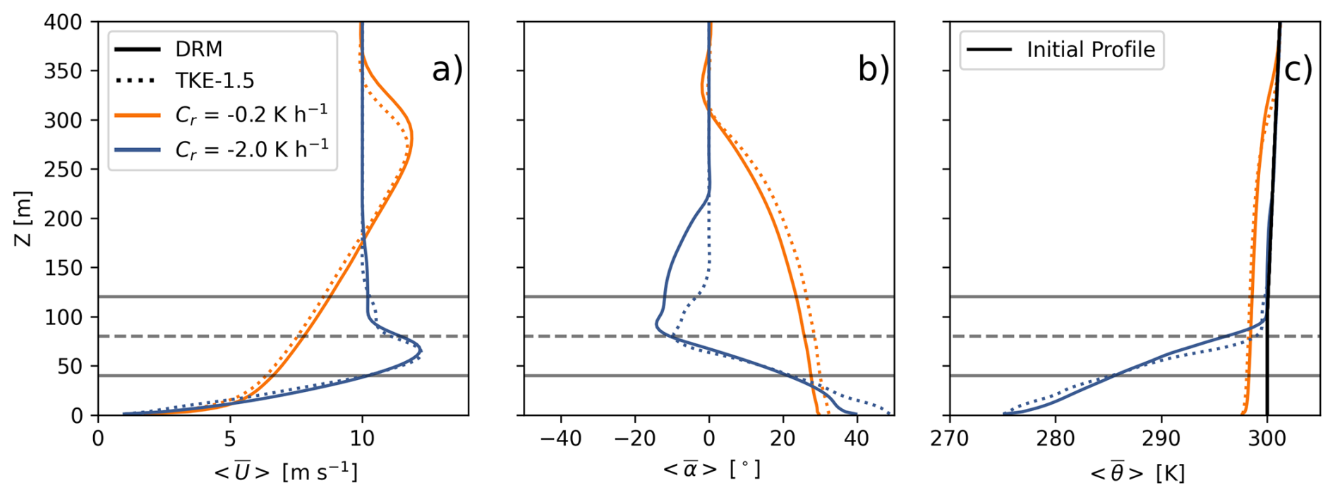
Figure 2 Planar- and time-averaged vertical profiles of (a) wind speed U, (b) wind direction α, and (c) potential temperature θ for the DRM and TKE-1.5 closures at 8 m resolution. Note that the results shown are for the outer domain without wind turbines. The solid horizontal lines represent the bottom and top of the rotor layer, while the dashed line represents hub height.

The thermally stable boundary layer develops as a strong potential temperature gradient forms from the ground up to the free atmosphere. In the free atmosphere, the 4 K km⁻¹ gradient initially imposed above 100 m persists due to a lack of turbulent mixing in the upper atmosphere. As such, for this case, downward entrainment into the wind farm is especially significant (see Sect. 3.3). The temperature profiles with the different cooling rates are shown in Fig. 2c, with the surface cooling over 26 K for the strongly stable regime but less than 5 K for the weakly stable case. The height of the stable layer depends on the cooling rate and the choice of the turbulence model, with the stable layer being deeper for the DRM closure compared to the TKE-1.5 closure. This difference is consistent with previous comparisons of the TKE-1.5 and DRM closures in the SBL (Zhou and Chow, 2012). Additionally, the dependence of SBL height on turbulence closure is documented in the GABLS study (Beare et al., 2006).

Figure 3 shows the planar- and time-averaged profiles of heat flux normalized by the heat flux value at the surface. (For the DRM closure, the surface heat flux values are −0.017 and −0.040 K m s⁻¹ for the weakly and strongly stable regimes, respectively, and for TKE-1.5, the values are −0.012 and −0.041 K m s⁻¹.) The resolved fluxes are small near the surface, and the turbulent fluxes are modeled by the turbulence closure. Above this region and within the SBL, the resolved fluxes reach a maximum and then decrease as buoyancy suppresses turbulence scales. For the weakly stable regime, the differences between two closures is relatively small, with both the DRM and TKE-1.5 closures resolving similar amounts of heat flux within the SBL. For the strongly stable regime, a much larger percentage (nearly 3 times higher) of the heat flux is resolved in the boundary layer for the DRM closure compared to results with the TKE-1.5 closure. For further analysis on the resolved and model heat fluxes between the two closures and at additional grid resolutions, see Appendix A.

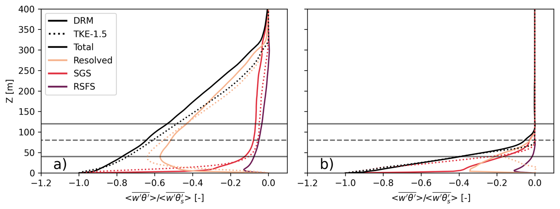
Figure 3 Planar- and time-averaged vertical profiles of normalized heat flux for the (a) weakly stable and (b) strongly stable regime for the DRM and TKE-1.5 closures at 8 m resolution. Note that the results shown are for the outer domain without wind turbines. The solid horizontal lines represent the bottom and top of the rotor layer, while the dashed line represents hub height.

One of the benefits of the DRM is that it allows backscatter of energy from subfilter scales to resolved scales. This effect can be quantified by calculating the SFS dissipation rate $\mathit{ϵ}=-{\mathit{\tau }}_{ij}{\stackrel{\mathrm{‾}}{\stackrel{\mathrm{̃}}{S}}}_{ij}$. Figure 4 shows a histogram of the SFS dissipation rates for the TKE-1.5 and DRM closures at heights of 50 and 80 m above the ground for the 8 m resolution strongly stable regime. As expected, the histograms of dissipation rate are entirely positive for the TKE-1.5 closure because it is an eddy-viscosity model. For the DRM closure, approximately 20 % and 40 % of the SFS dissipation rate values are negative at z=50 m and z=80 m, respectively, indicating backscatter. Traditional eddy-viscosity closures are known to be overly dissipative (Carper and Porté-Agel, 2004; Sullivan et al., 2003), and backscatter has been shown to be important, especially in stably stratified flows (Mason and Thomson, 1992; Kosović, 1997). Backscatter was also seen in Zhou and Chow (2011) and matches turbulence measurements in the atmospheric surface layer (Carper and Porté-Agel, 2004).

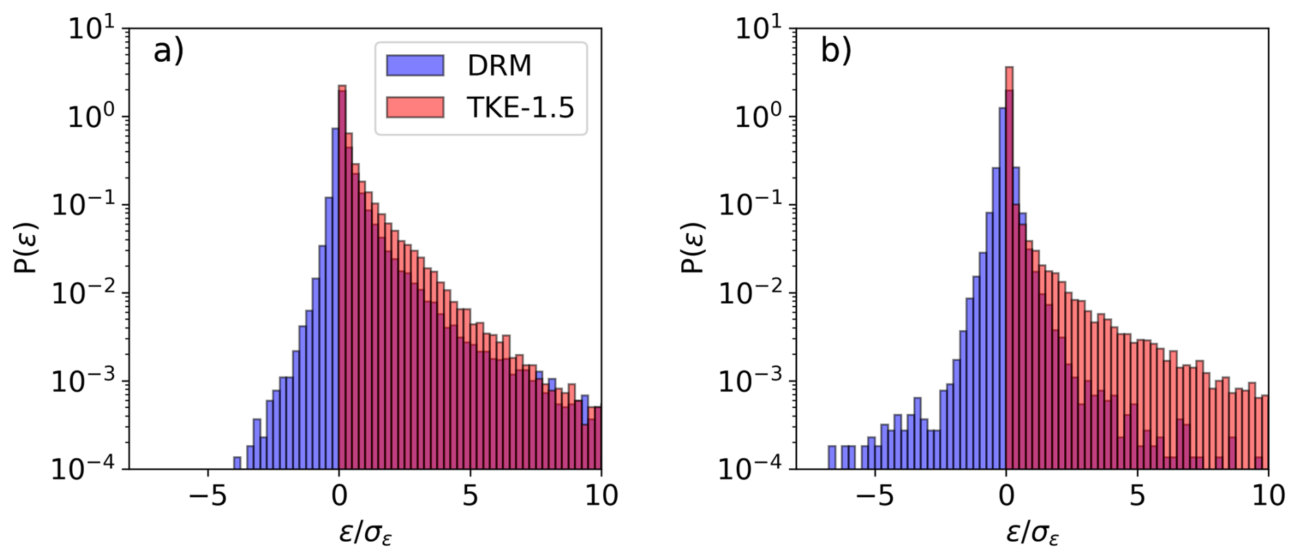
Figure 4 Distribution of subfilter-scale turbulent dissipation rates for the TKE-1.5 and DRM closures at (a) z = 50 m and (b) hub height (z = 80 m) on the outer domain for the strongly stable regimes. The turbulence dissipation rate ϵ is normalized by its standard deviation σ_ϵ at the given height. Negative values represent the backscatter of turbulent energy from the subfilter scales to the resolved scales.

The ability of the DRM closure to physically represent backscatter leads to an improved representation of turbulence under strong stability compared to the TKE-1.5 closure, especially at the relatively coarse 8 m grid spacing. Figure 5 shows the planar- and time-averaged vertical profiles of the normalized total momentum flux as well as the percentage of backscatter in the SFS dissipation rate as a function of height for the DRM closure for both stability regimes and at 8 m horizontal grid spacing. (The magnitudes of the surface momentum flux values are 0.30 and 0.14 m² s⁻² for the weakly and strongly stable regimes, respectively.) The momentum flux profiles in Fig. 5 are also shown with conditional averaging based on the sign of the SFS dissipation. In the strong-stability case, local backscatter events (where ϵ<0) result in smaller-magnitude momentum fluxes compared to the fluxes in areas of positive SFS dissipation (ϵ>0). For the weak-stability case, the magnitude of the momentum fluxes is more similar for backscatter and dissipation events. Lastly, for both stability regimes, the momentum fluxes at the top of the boundary layer and within the LLJ are of similar magnitude but with opposite signs during backscatter and dissipation events. The fluxes when ϵ>0 are balanced by the fluxes when ϵ<0 as the contributions from backscatter and positive SFS dissipation are roughly equal at the top of the boundary layer.

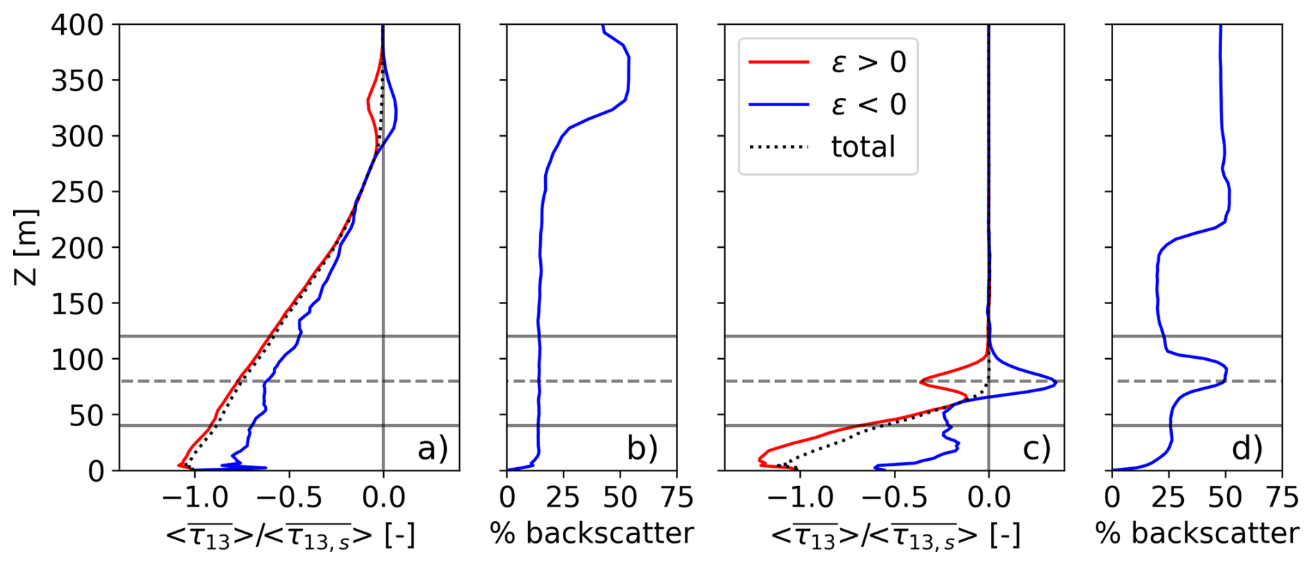
Figure 5 Planar- and time-averaged vertical profiles of normalized total momentum flux (resolved + modeled) for the (a) weakly stable and (c) strongly stable regime for the DRM closure at 8 m resolution conditionally averaged based on the sign of the SFS dissipation rate (negative indicating backscatter). Percentage of backscatter in the SFS dissipation rate for a given height for the (b) weakly and (d) strongly stable regimes. Note that the results shown are for the outer domain without wind turbines. The solid horizontal lines represent the bottom and top of the rotor layer, while the dashed line represents hub height.

Using the DRM closure at 8 m grid spacing provides a computationally efficient framework for simulating a domain large enough to analyze wind turbine and farm wake effects under strongly stable conditions (see Appendix A for analysis regarding computational cost between the two closures). Hereinafter, all results presented use the DRM closure.

3.2 Quantifying intermittency

There are multiple definitions of turbulence intermittency in the atmosphere, with this study focusing on global intermittency. Holtslag and Nieuwstadt (1986) remark that for global intermittency, turbulence is weak and not continuous in time and space, with turbulence confined to isolated patches that develop and disappear. We use scaling to initially characterize the behavior (continuous vs. intermittent) of the simulated stable boundary layers. Holtslag and Nieuwstadt (1986) identified scaling parameters to define a criterion in which the SBL displays intermittent behavior at a given height. Their criterion depends on the boundary layer height h and the Obukhov length L and defines when stability is strong relative to mechanical forcing, with large $h/L$ indicating a very stable regime where turbulence becomes intermittent and difficult to sustain, especially aloft. For smaller $h/L$, buoyancy suppression is weaker relative to mechanical forcing resulting in sustained, continuous turbulence through much of the boundary layer. The boundary layer height can be determined using their definition, which is the height to which turbulence extends above the surface. Here, we calculate h by determining the height at which the heat flux goes to less than 1 % of the surface value (see Fig. 3).

The boundary layer height for the strongly stable regime is determined to be 105 m. The inverse Obukhov length is formulated as $L^{-\mathrm{1}}=-\mathit{\kappa }\left(g/{\mathit{\theta }}_{\text{sfc}}\right)H/u_{*,\text{sfc}}^{\mathrm{3}}$, where $u_{*,\text{sfc}}$ is the surface friction velocity, H is the surface heat flux, κ is the von Kármán constant (taken as 0.4), g is the gravitational constant, and θ_sfc is the potential temperature at the surface. The average inverse Obukhov length is then taken over the analysis period. Note that we use this formulation as opposed to averaging the individual quantities that make up L due to the non-linear influence of the surface fluxes in the similarity functions, as demonstrated by Kelly and Gryning (2010). The inverse Obukhov length is calculated to be 0.172 m⁻¹ for the strongly stable regime, resulting in $h/L=\mathrm{18}$, thus confirming that the strongly stable regime is intermittent, as defined in Fig. 2 of Holtslag and Nieuwstadt (1986). For the weakly stable regime, h=398 m and $L^{-\mathrm{1}}=\mathrm{0.007}$m⁻¹, resulting in $h/L=\mathrm{3}$, which is in the region of continuous turbulence. See Holtslag and Nieuwstadt (1986) for additional details on scaling in the SBL.

Furthermore, the Obukhov length L can be defined at a specified height above the surface, which is commonly done when characterizing the climatology of field sites. For the AWAKEN region, Krishnamurthy et al. (2021) calculated the Obukhov length at 25 m above the ground and found that very stable conditions ($\mathrm{10}<L<\mathrm{50}$) occurred approximately 20 % of the time from 2012–2019 (see Figs. 14 and 15 in Krishnamurthy et al., 2021). For our study, we can similarly calculate L using the previously mentioned formulation but by replacing H with the resolved heat flux $w^{\prime }{\mathit{\theta }}^{\prime }$ at 25 m, where w^′ and θ^′ are the fluctuating components of the vertical velocity and potential temperature obtained by removing a running 30 min mean (the same time window used in Krishnamurthy et al., 2021). For the strongly stable regime, the average Obukhov length calculated using this method is 36.9 m, which is within the window defined in Krishnamurthy et al. (2021) for strongly stable conditions. This comparison demonstrates that the strongly stable case considered here is entirely plausible in the AWAKEN region.

To quantitatively describe the intermittent turbulence visible in the strongly stable case at a given height, we follow a similar approach to that used by Coulter and Doran (Coulter and Doran, 2002), who used heat flux measurements from sonic anemometer data during the CASES-99 field campaign. We apply their methodology but use TKE as the metric of interest as our goal is to identify turbulent periods. At the virtual tower, TKE is defined as $\frac{\mathrm{1}}{\mathrm{2}}({u^{\prime }}^{\mathrm{2}}+{v^{\prime }}^{\mathrm{2}}+{w^{\prime }}^{\mathrm{2}})$, where u^′, v^′, and w^′ are the fluctuating components of the velocities obtained by removing a running 30 s mean, as we are focused on small-scale turbulence, and then averaged again over a 1 min interval to further smooth the data (shown in Fig. 6a at various heights). Then the values in the TKE time series are sorted from largest to smallest to obtain a cumulative probability distribution.

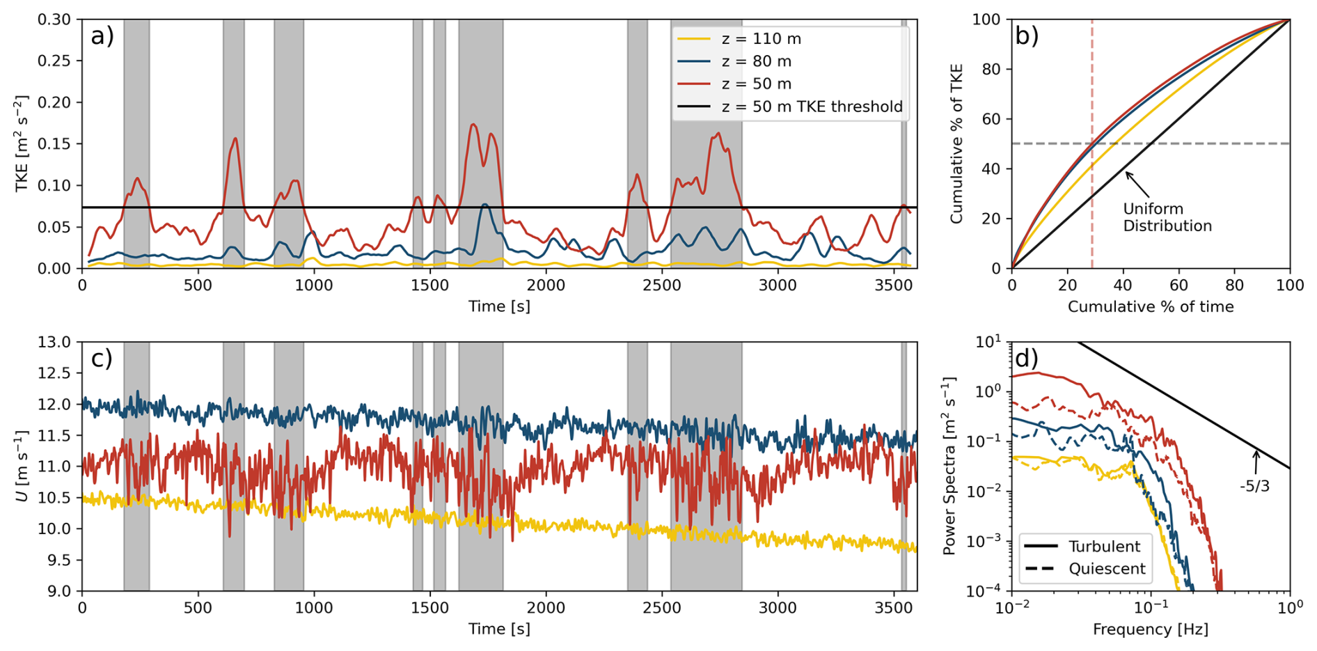
Figure 6 (a) Time series and (b) cumulative distribution function of TKE at various heights within the rotor disk for the strongly stable regime 5D upwind of the wind farm on the inner domain. (c) Time series and (d) power spectra of wind speed at the same heights as in (a) and (b). The dashed lines in (b) pinpoint the cumulative percentage of time it takes until 50 % of the TKE occurs at a height of 50 m. The periods highlighted in gray are “turbulent”, while other periods are “quiescent”. In (d), the $-\mathrm{5}/\mathrm{3}$ inertial subrange power law is provided in black for reference.

The cumulative probability distribution of the sorted TKE at various heights within the rotor plane for the strongly stable regime is shown in Fig. 6b. The black diagonal line represents the distribution if the TKE were distributed uniformly during the analysis period; i.e., 50 % of the TKE would occur in 50 % of the analysis period. We extend Coulter and Doran's (Coulter and Doran, 2002) definition of “intermittency fraction” to TKE (from heat flux) such that it represents the first 50 % of the sorted TKE signal. It should be noted that TKE cannot be uniformly distributed since it is defined itself by fluctuations, so there will always be some level of skewness, and the intermittency fraction must be less than 50 %. For the strongly stable regime, the intermittency fraction is 30 % at hub height and 29 % at z = 50 m, meaning that 50 % of the total TKE during the analysis period happens in just 30 % of the analysis time. In the upper portion of the rotor plane, the intermittency fraction is closer to 40 %. An intermittency fraction of 29 % is consistent with the <30 % intermittency fractions observed during many of the strongly stable nights analyzed by Coulter and Doran (Coulter and Doran, 2002) during CASES99 (although they also saw nights with smaller intermittency fractions) and simulation results during strongly stable conditions from Zhou and Chow (2012). Similarly, in their simulations, van der Linden et al. (2020) found their SBL regime to be in a turbulent or bursting state 26 % of the time, although they used a different metric to quantify intermittency. However, note that the results in this study do not provide a direct comparison since TKE is the metric used, whereas the others used heat flux.

The analysis period is further subdivided into quiescent and turbulent periods. Figure 6a and c show time series of the wind speed and TKE at z=50, 80, and 110 m, where periods with intermittency are highlighted in gray and denoted as “turbulent” periods, while other periods are referred to as “quiescent” periods. We can qualitatively see large fluctuations in both the wind speed and TKE during the turbulent periods at 50 m. At 80 m (hub height) and 110 m, the fluctuations are not as qualitatively evident. We use turbulence intensity (TI), calculated as $\text{TI}={\mathit{\sigma }}_U/U_{\text{mean}}$, with σ_U as the standard deviation of U, to quantify the differences in turbulence during the quiescent and turbulent periods. At 50 m, the TI is 3.5 % during the turbulent periods and only 2.2 % during quiescent periods. Considering the relatively small TIs typical during SBL conditions, these differences in TI during quiescent and turbulent periods are significant, as discussed later. Note that at both 80 and 110 m, the wind speed slowly decreases in time due to multi-hour (∼18.7 h at a latitude of 40°) inertial oscillations at the Coriolis frequency.

Increased levels of turbulence during turbulent periods, as compared to quiescent periods, are also clear when plotting the power spectral density (PSD) of the wind speeds at the three heights, as shown in Fig. 6d. The wind speed signals have been separated by turbulent and quiescent periods, as indicated by the shaded gray regions in Fig. 6c. The PSDs are calculated for each distinct turbulent or quiescent period and then averaged. At 50 m, the energy content is increased across all frequencies during the turbulent periods compared with the quiescent periods. There is a much smaller difference in the energy content at the higher frequencies for heights of 80 and 110 m. In Fig. 6d, as height increases, the width of the $-\mathrm{5}/\mathrm{3}$ inertial subrange decreases. The time series at 80 m is within the nose of the LLJ, and the time series at 110 m is above the LLJ. At both of these heights, turbulence is very weak, so the spectra exhibit little to no inertial subrange, which is another reason why the difference in the energy content between quiescent and turbulent periods at these heights is small. Furthermore, the additional energy content for only the lower half of the rotor disk along with the intense, vertical wind shear could lead to increased blade fatigue as discussed by Kelley et al. (2006).

The shape of the distribution of turbulence can be used as an additional metric to confirm intermittency in the strongly stable regime. While we expect the distribution for continuous turbulence to be roughly Gaussian (i.e., with one peak), for intermittent turbulence we expect the distribution to be bimodal. Figure 7 shows the time series of TKE for both the weakly and strongly stable regimes at 70 % of the boundary layer height (50 $\mathrm{m}\mathrm{a}.\mathrm{g}.\mathrm{l}.$ for the strongly stable regime), with the distributions of the TKE signal also provided. As expected for the strongly stable regime, the distribution of turbulence is more bimodal than in the weakly stable regime. The majority of the turbulence occurs around a value of 0.05 m² s⁻², with a second, smaller peak around 0.15 m² s⁻¹, which is roughly 3 times as large. To quantify bimodality, we use Sarle's bimodality coefficient, with coefficients larger than $\mathrm{5}/\mathrm{9}$ (0.555) considered to be bimodal (Ellison, 1987). The bimodality coefficient for the distribution of turbulence for the strongly stable regime is 0.63, while it is 0.45 for the weakly stable regime. This result further confirms the intermittent nature of the turbulence in the strongly stable case.

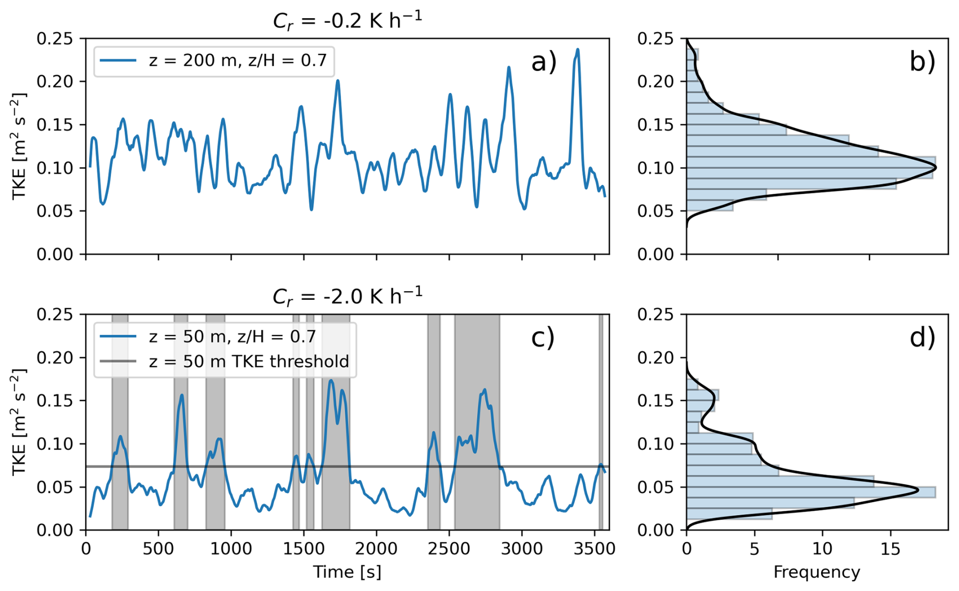
Figure 7 Time series of TKE at 70 % of the boundary layer height for the (a) weakly and (c) strongly stable regimes. Histogram of the TKE distribution for the (b) weakly and (d) strongly stable regimes. The black lines in (b) and (d) represent kernel density estimates of the probability distribution functions. In (c), the periods highlighted in gray are “turbulent”, while other periods are “quiescent”.

Lastly, plan views of TKE qualitatively demonstrate the spatial organization of intermittent turbulence. Figure 8 shows time instances of TKE at 70 % of the boundary layer height at the beginning of the analysis period for the weakly and strongly stable regimes. The TKE is computed as $\text{TKE}=\frac{\mathrm{1}}{\mathrm{2}}({u^{\prime }}^{\mathrm{2}}+{v^{\prime }}^{\mathrm{2}}+{w^{\prime }}^{\mathrm{2}})$, where u^′, v^′, and w^′ are the fluctuating components of the velocities obtained by removing the planar average, e.g., $u^{\prime }=u-\langle u\rangle$, where 〈u〉 is the planar average for the specific time instance. For the weakly stable regime (Fig. 8a), the TKE signal exhibits small-scale turbulent structures distributed evenly throughout the domain. When using the DRM closure at a horizontal grid spacing of 8 m, the strongly stable regime shows patches of increased TKE and more quiescent regions with very little TKE. These patches continuously develop in different locations throughout the analysis period as result of shear cyclically increasing and decreasing. The patchiness in Fig. 8b shows qualitative similarities to observations (Mayor et al., 2012) and direct numerical simulations (Ansorge and Mellado, 2014, 2016) of intermittent turbulence.

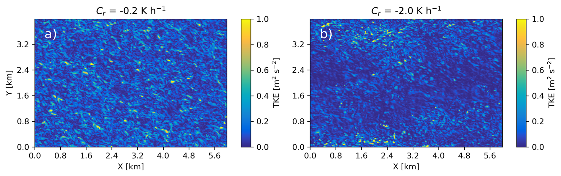
Figure 8 Instantaneous plan view of TKE at the beginning of the analysis period for the (a) weakly stable regime at 200 $\mathrm{m}\mathrm{a}.\mathrm{g}.\mathrm{l}.$ and (b) strongly stable regime at 50 $\mathrm{m}\mathrm{a}.\mathrm{g}.\mathrm{l}.$ Note that both heights correspond to 70 % of the boundary layer height for each regime.

3.3 Effect of wind farms on the stable boundary layer

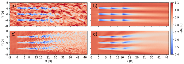
The presence of a wind farm has different effects on the atmospheric boundary layer for each stability regime. Figure 9 shows plan views of instantaneous and time-averaged hub-height velocity deficits. The velocity deficit is calculated as the difference in the wind field from the velocity 5D upwind of the first row of turbines, with the reference or freestream value being averaged in the spanwise direction (from −5D to 5D) to account for the width of the farm. In the instantaneous slice in Fig. 9a, turbulent structures are generally evenly distributed in the weakly stable regimes. For the strongly stable regime in Fig. 9c, the hub height is just above the nose of the LLJ, and thus much less turbulence is expected. For the instance shown in Fig. 9c, there are no turbulent structures in the inflow other than some very faint wave-like structures.

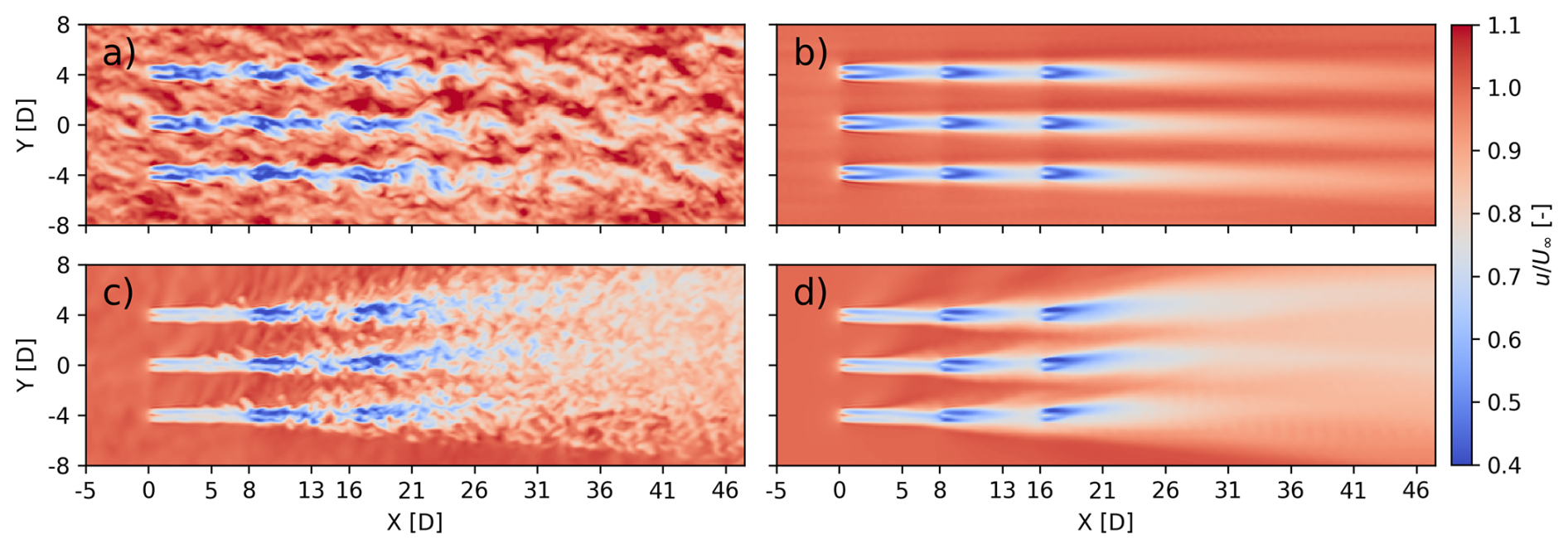
Figure 9 Instantaneous (a, c) and 1 h time-averaged (b, d) plan view of velocity deficits at hub height for the weakly (a, b) and strongly (c, d) stable regimes.

For both regimes, the wind turbine wakes propagate over 30D downwind, as seen in the time averages in Fig. 9b and d. The considerable wind veer also results in the lateral spreading of the wakes, which depends on wind directions at heights where momentum is entrained from, as discussed by van der Laan and Sørensen (2017). As expected, the velocity deficits are more pronounced downwind within the wind farm as the second and third rows are waked by upwind turbines. Wakes and velocity deficits depend on the operating turbine's thrust coefficient and are thus strongly dependent on the incoming hub-height wind speed. The velocity deficits for the first row of turbines are dependent on the incoming wind speeds, which are 7.8 and 11.6 m s⁻¹ for the weak- and strong-stability regimes, respectively. In general, wind turbines (and specifically the turbine used in this study) have higher thrust coefficients at slower wind speeds, which then decrease as the wind speed increases. As a result, the velocity deficit for the first row of turbines in the farm is strongest for the weakly stable regime and weakest for the strongly stable regime. The downwind turbines within the farm have stronger wake deficits compared to the first row for both stability regimes due to the lower wind speed and thus higher thrust coefficients that these turbines experience.

The vertical structure of the wake deficits persists for over 30D downwind and depends strongly on the height of the LLJ. Time-averaged vertical transects of wind speed aligned with the middle of the wind farm are shown in Fig. 10a and b for both stability regimes. The wakes of the turbines are a cumulative effect of individual wind turbine wakes morphing into a wind farm wake, which is consistent with observations of wind farm wakes during SBL conditions (Hirth and Schroeder, 2013). Additionally, these cumulative wakes can adversely affect downwind wind farms (Lundquist et al., 2019). The effect of the wind farm wake is most clear for the strongly stable regime, where slower wind speeds above the LLJ nose persist downwind. At altitudes within and below the LLJ, the wake recovers relatively quickly because of the ambient turbulence; however, above the LLJ, where turbulence levels are low, the wake recovers extremely slowly. Of course, the altitude of the LLJ, and therefore the wake recovery, is dictated by the stability. The average inflow TKE value at 50 m for the strongly stable regime is 0.086 m² s⁻², while it is 0.032 m² s⁻² at 80 m and just 0.004 m² s⁻² at 110 m.

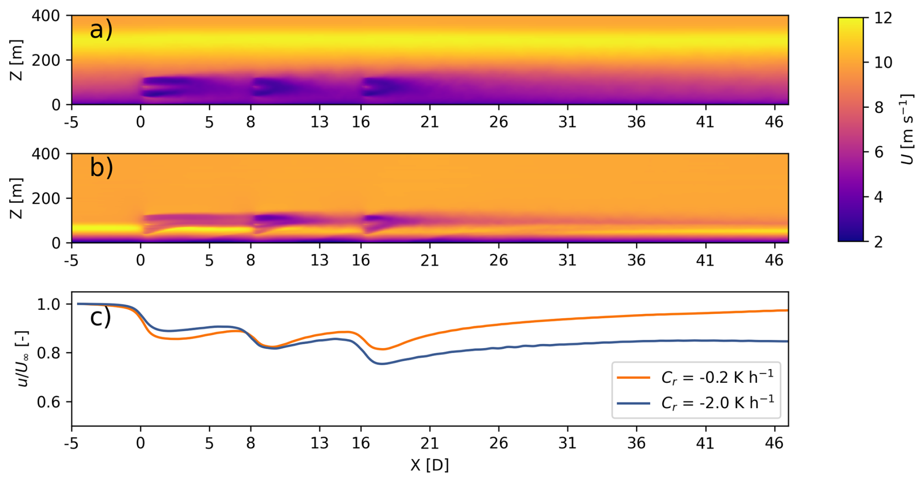
Figure 10 Time-averaged vertical transect of wind speed for the (a) weakly and (b) strongly stable regimes. (c) Hub-height wind speed as a streamwise distance normalized by the wind speed 5D upwind of the first row of turbines for each stability regime. For (c), the wind speed is averaged in the spanwise direction (−5D to 5D) to account for the three turbines in each row within the wind farm.

The slow recovery of velocities downwind of the farm in the strongly stable regime is also evident in Fig. 10c, which shows hub-height wind speed normalized by the wind speed at −5D, also with averaging in the spanwise direction to account for the width of the farm. The initial decrease in wind speed after the first row of turbines is greatest at 15 % for the weakly stable regime; however, the greatest decrease in wind speed at the end of the farm is for the strongly stable regime, where the deficit is 25 % after the third row of turbines. These trends are similar to those observed by Gadde and Stevens (Gadde and Stevens, 2021a), who saw that wake deficits for farms that interact with LLJs are greatest when the LLJ height is similar to the hub height. For the strongly stable case, when the LLJ height is similar to a wind turbine's hub height, momentum transfer (entrainment) is reduced because the LLJ structure is significantly impacted by the drag of the wind turbine rotors. Any entrainment for this case must come from the slower wind speeds above or below the LLJ. In contrast, for the weakly stable case, entrainment from the faster wind speeds in the LLJ nose above the rotor disk aids in wake recovery.

Intermittent turbulence in the inflow for the strongly stable regime is overpowered by the wake-added turbulence from the wind farm. Figure 11 shows the cumulative distribution functions of sorted TKE at locations of 5D upwind ($x=-\mathrm{5}D$) and 10D downwind (x = 26D) of the wind farm for both stability regimes at 50 m above the ground. The intermittency fraction for the weakly stable regime is close to 40 %, while for the strongly stable regime, the intermittency fraction is 29 %. As previously mentioned, this means that the strongly stable regime is turbulent only in bursts at this height, while for the weakly stable regime, the turbulence is continuous and nearly uniform. Downwind of the wind farm, the intermittency fraction for both stability regimes is similarly close to 40 %, indicating that wake-added turbulence now drives the distribution of turbulence. Wake-added turbulence is continuous throughout the hour-long period, i.e., without distinct periods of turbulence intermittency. The mean TKE value over the hour-long period at this height for the strongly stable case is 0.09 m² s⁻² upwind of the farm, while it is 0.40 m² s⁻² 10D downwind of the farm. Therefore, ambient turbulence is smaller compared to contributions from the wake in the strongly stable regime.

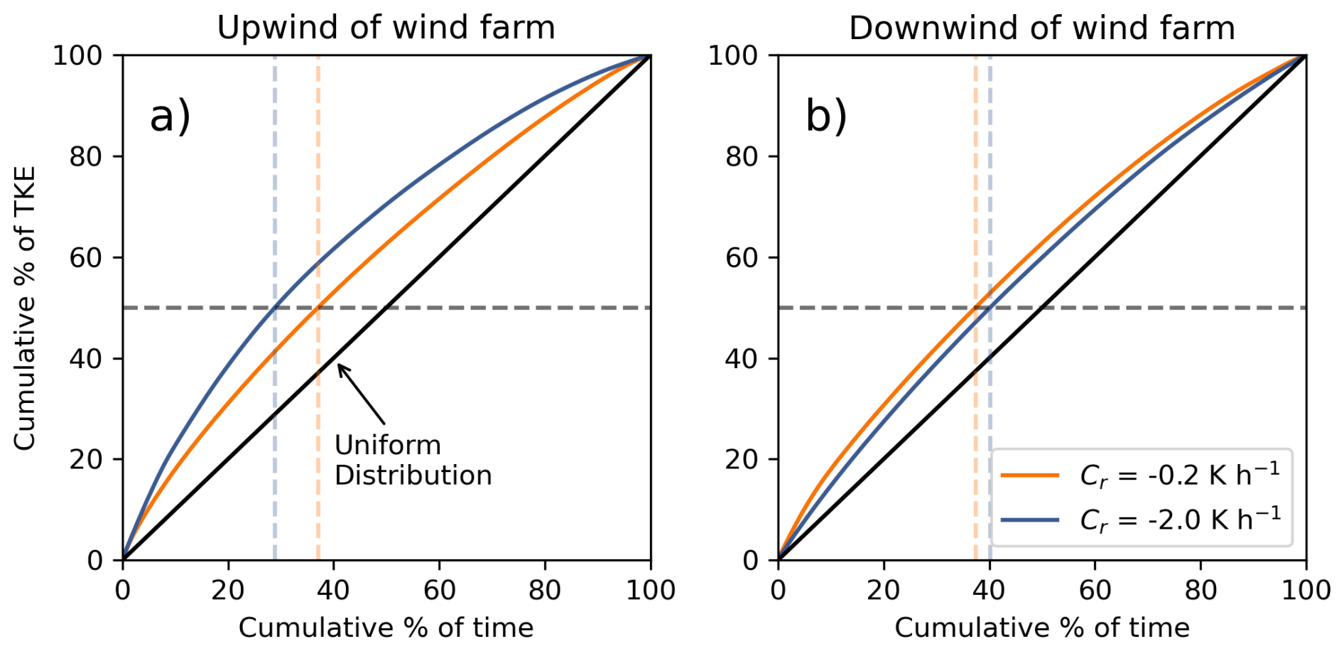
Figure 11 Cumulative distribution function of TKE (a) 5D upwind ($x=-\mathrm{5}D$) and (b) 10D downwind (x=26D) of the wind farm for each stability regime at z = 50 m. The dashed lines pinpoint the cumulative percentage of time it takes until 50 % of the TKE occurs.

The added TKE from the farm impacts the SBL in a number of ways. Figure 12a and b show wind speed and momentum flux averaged across the spanwise transects in Fig. 1 at 5D upwind ($x=-\mathrm{5}D$) and 5D downwind of the farm (x = 21D) for both stability regimes. The momentum flux is normalized by the value at the surface for each individual case. For both regimes, the velocity deficit due to the wind farm wake is evident in reduced velocities within the rotor layer. The wind speeds are also decreased above the rotor layer because momentum is entrained into the wake from above, as indicated by negative momentum flux values in Fig. 12b. For the strongly stable regime, the momentum flux is mostly positive in the bottom half of the rotor disk, indicating that momentum is transferred from below, and this is because the nose of the LLJ is slightly below hub height, and the upper half of the rotor disk is in the negative shear region. This entrainment from below that aids in wake recovery agrees with modeling results from other work (Gadde and Stevens, 2021b). Additionally, see van der Laan et al. (2023) for additional discussion regarding wake recovery mechanisms.

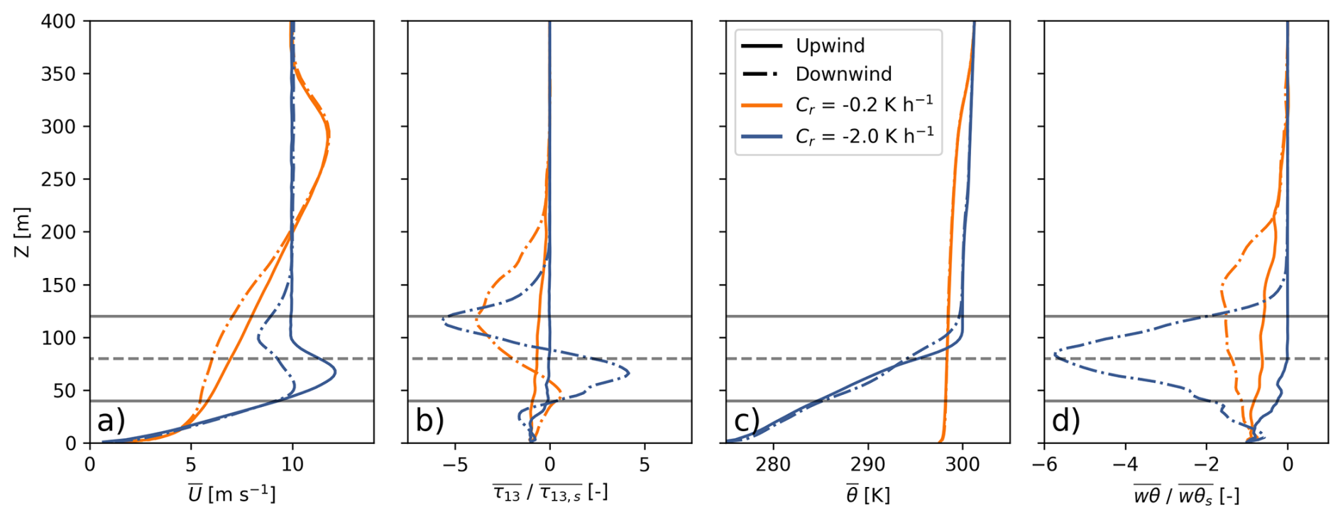
Figure 12 Vertical profiles of (a) wind speed, (b) streamwise vertical momentum flux, (c) potential temperature, and (d) vertical heat flux 5D upwind ($x=-\mathrm{5}D$) and 5D downwind (x = 21D) of the farm for each stability regime. The solid horizontal lines represent the bottom and top of the rotor layer, while the dashed line represents hub height.

The wakes also affect the thermodynamic characteristics of the stable layers. The spanwise-averaged potential temperature and heat flux are shown in Fig. 12c and d, respectively. The depth of the stable layer increases, and the temperature gradient is reduced across the rotor disk most prominently for the strongly stable regime. For both stability regimes, the heat flux is negative throughout the vertical profile, indicating that warmer air is entrained from above. The wind-farm-induced change in stratification is also visible in Fig. 13, which shows the spanwise-averaged change in temperature (compared to −5D) as a function of height at various streamwise locations. For the strongly stable regime, the temperature decreases in the upper half of the rotor disk and increases in the lower half of the rotor disk. Similar trends hold for the weakly stable regimes but centered around the top of the rotor disk, although the changes in temperature are much smaller for the weakly stable regime. The wind farm, in effect, creates a less stable layer from the ground to the top of the rotor disk and even up to 80 m above the rotor disk for the weakly stable regime. These wind-farm-induced effects on the SBL persist over 30D downwind of the farm.

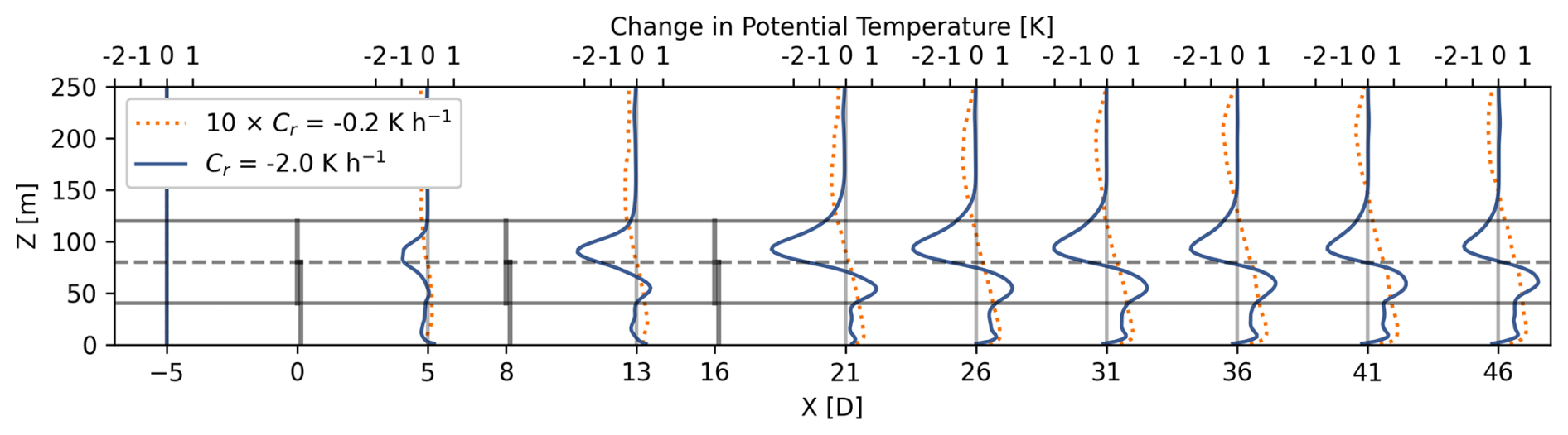
Figure 13 Spanwise-averaged profiles for the change in potential temperature at various distances (relative to $x=-\mathrm{5}D$) for each stability regime. Note that the profiles for the weakly stable regime have been amplified by a factor of 10 for visualization purposes. The solid horizontal lines represent the bottom and top of the rotor layer, while the dashed line represents hub height.

3.4 Effect of intermittent turbulence on farm performance

Considering the intermittent turbulence present in the strongly stable regime, the following work aims to understand and quantify how intermittency affects wind turbine wake recovery as well as power production. To examine the flow structure during turbulent and quiescent periods for the strongly stable regime, we look at plan slices of the velocity deficit and TKE at 50 m above the ground. Figure 14a and c show a quiescent instance of velocity deficit and TKE, while Fig. 14b and d show a turbulent instance. Note that the colorbar in Fig. 14c and d is truncated at a maximum value of 2.0 m² s⁻² so that the inflow turbulence is more pronounced; there are higher values downwind due to wake-added turbulence, which are not apparent with this colorbar. For the turbulent instance, smaller coherent structures are visible in the velocity deficits upwind of the first row of turbines as well as between the first and second row of turbines. These structures represent coherent turbulent eddies and are evident in the plan slice of TKE in Fig. 14d.

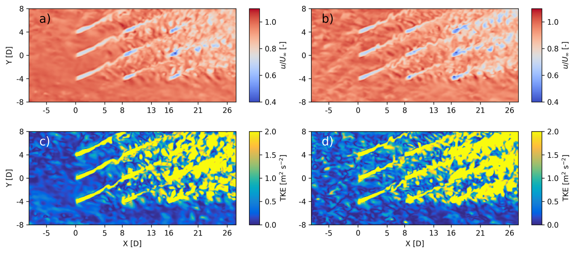
Figure 14 Example (a, c) quiescent and (b, d) turbulent instantaneous plan view of (a, b) velocity deficits and (c, d) TKE at 50 m above the ground for the strongly stable regime.

The TKE is up to 10 times higher during turbulent periods compared to quiescent periods. However, the turbulent periods have little effect on wake recovery as downwind of the turbines, turbulence is largely wake-generated. Figure 15 shows the spanwise-averaged (−5D to 5D) velocity deficit profiles within the wind farm and downwind of the wind farm. The velocity deficit profiles have been separated by whether the flow is more turbulent or quiescent using the procedure described in Sect. 3.2. The velocity deficits are nearly identical regardless of the streamwise location. This is because, while the TKE is much larger during turbulent periods compared to quiescent periods, the TKE during the turbulent periods is still very small when compared to the weak-stability regime or to the wake-added turbulence from the wind turbines. The larger turbulence during the intermittent turbulence does not aid in wake mixing since turbulence levels are so small, and thus the velocity deficits are only marginally impacted, as seen by the solid and dashed lines nearly overlapping in Fig. 15.

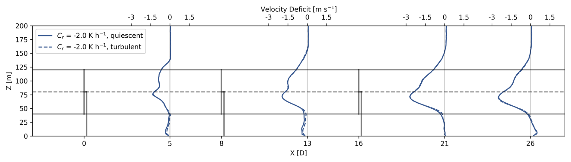
Figure 15 Velocity deficit profiles at various streamwise locations (relative to $x=-\mathrm{5}D$) separated by quiescent and turbulent periods for the strongly stable regime. The solid horizontal lines represent the bottom and top of the rotor layer, while the dashed line represents hub height.

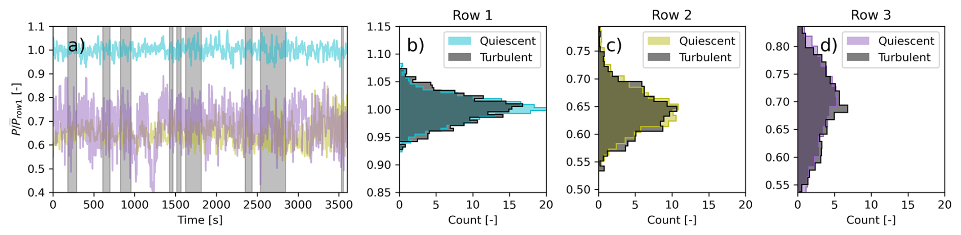
The intermittent turbulence resolved in this study does not significantly affect the average power production but does have a small effect on the power variability in the wind farm during the strongly stable regime. Figure 16a shows the time series of the average power production during the analysis period for each row of turbines within the farm, normalized by the rated power, with turbulent periods highlighted in gray. Figure 16b–d show histograms of the power production to provide insight into the spread for each row. Note that the turbine used in this study can produce power greater than its rated power (greater than 1 in Fig. 16a) for wind speeds in the range of 10–13 m s⁻¹, as discussed in Arthur et al. (2020), which impacts the distribution of the power signal. The first row sees the largest difference in variability, with a standard deviation of 45.7 kW during turbulent periods and 40.8 kW during quiescent periods, or a roughly 13 % increase in the power variability. Regarding average power, the front-row performance is largely unchanged during quiescent and turbulent periods (1712 vs. 1713 kW) as differences in the mean wind speeds are very small for the different periods. For the second and third rows, average power and power variability are largely independent of intermittent turbulence for the same reasons as described above (their inflow is dominated by characteristics of upwind wakes).

Figure 16 Time series (a) and histograms by row (b–d) of detrended power normalized by the rated power of the turbine for the strongly stable regime. The periods highlighted in gray are turbulent, while periods in white are quiescent, as determined by the method in Sect. 3.2.

4 Conclusions

In this study, the WRF-LES-GAD framework is used to provide insight into how wind farms interact with extreme and less common, strongly stable atmospheric conditions in contrast with more typical, weakly stable conditions. The primary focus is to determine (1) how the presence of wind turbine wakes affects stable boundary layer evolution and (2) how the intermittent turbulence in strongly stable boundary layers affects power production and wake recovery. A one-way nested approach is used with idealized LES, where turbulence is spun up on the outer domain using doubly periodic lateral boundary conditions. The outer domain provided forcing for the inner domain containing a 3×3 wind farm consisting of nine 1.6 MW turbines. The grid spacing was the same in each domain, meaning that the fully developed turbulent structures from the periodic outer domain are passed directly into the inner domain.

The explicit filtering framework and dynamic reconstruction turbulence model of Chow et al. (2005) is used to extend the working range of LES in the stable boundary layer, and, as a result, turbine–airflow interactions can be studied in such strongly stable conditions with realistic turbulence. The development of the boundary layer on the outer domain was first compared between the DRM closure and the commonly used TKE-1.5 closure. The percentage of vertically integrated resolved heat flux of the total heat flux was similar across both closures at a relatively coarse 8 m horizontal resolution for the weakly stable regime. However, for the strongly stable regime, the DRM closure resolved a larger fraction of the heat flux compared to the TKE-1.5 closure, indicating improved representation of heat flux (and, by extension, other turbulence quantities) in the resolved flow field. The TKE-1.5 closure is entirely dissipative by nature, while the DRM closure is able to physically represent the backscatter of turbulence from smaller scales to larger scales, which was shown to be especially important as it relates to the momentum flux in strongly stable boundary layers.

For both stability conditions, the imposed forcing resulted in a LLJ at the top of the stable layer, with the height of the jet relative to the turbine having a major impact on the SBL evolution downwind. The height of this jet decreased with increasing stability, with the jet being above the rotor disk for the weakly stable regime and just below hub height for the strongly stable regime. Below the LLJ, continuous turbulence formed in the weakly stable regime, but turbulence occurred intermittently (in addition to background turbulence) for the strongly stable regime due to a balance between shear-generated turbulence and buoyancy suppression (Appendix B). The wind farm in the strongly stable regime experienced intermittent turbulence below hub height (50 % of the turbulence occurs in just 29 % of the simulation time) and very little turbulence along with a negative wind shear region in the upper half of the rotor disk. Downwind of the wind farm, the flow was no longer intermittent as the flow structures were dominated by continuous, wake-added turbulence. Additionally, momentum transfer was dependent on the altitude of the LLJ. For the strongly stable regime, momentum was largely transferred upwards from the LLJ below hub height to aid in wake recovery, whereas for the weakly stable regime, momentum was entrained from higher wind speeds within the LLJ aloft. Heat was always transferred downward from above for both stability regimes, resulting in a less stable layer downwind of the farm. While LLJs below hub height are uncommon, it is worth noting that as turbines continue to grow (Bilgili and Alphan, 2022), hub heights will more frequently extend into the free atmosphere, and better understanding of this behavior is needed for turbine design (Veers et al., 2023).

For the strongly stable regime, periods of elevated intermittent turbulence increased wind farm power variability but had little impact on the average power production. The standard deviation in the power output for the first row of turbines within the farm was 13 % higher during turbulent periods compared to quiescent periods. However, downwind rows were not affected by this power variability because the turbulence the downwind turbines experience was wake-added and thus more continuous. The focus of this study was on turbine power production; the impact of intermittent turbulence on structural loading is an avenue for future work.

Both the numerical methods and analyses used in this idealized study can be extended to the conditions observed during AWAKEN or other future field campaigns. In particular, the DRM closure provides a less computationally expensive framework for modeling the SBL and interaction with wind farms. Recently, the DRM closure has also been used in multi-scale WRF-LES-GAD simulations for AWAKEN, with realistic time-varying inflow conditions downscaled from reanalysis data while also incorporating topography (Wise et al., 2025). The intermittent turbulence explored in this study is a result of the competition between shear production and buoyancy suppression. Other mechanisms for SBL intermittency that are common in the US Southern Great Plains, the region for the AWAKEN field campaign, include bores, Kelvin–Helmholtz billows, terrain-induced flows (e.g., Radünz et al., 2025, for flow speedup and Zhou and Chow, 2014, for terrain-related shear-instability waves), and propagating density currents. While the intermittent turbulence simulated as part of this study had only a modest impact on wind farm performance, Wise et al. (2025) showed that another type of intermittent turbulence (gravity waves) can result in significant impacts on average power production and the power variability. Ultimately, this study demonstrated a methodology for identifying and quantifying intermittent turbulence events from a time series of TKE. These methods can be used in future work with observations from meteorological towers, vertical profiling lidars, and supervisory control and data acquisition (SCADA) data from AWAKEN to examine wind farm performance in various intermittent turbulence conditions.

Appendix A: Turbulence representation on different grids for the TKE-1.5 and DRM closures

The resolved and modeled heat fluxes can be used as a proxy to determine the percentage or fraction of resolved turbulence. This is done by calculating the vertically integrated resolved heat flux (q) divided by the vertically integrated total heat flux (Q). This quantity provides insight into whether the turbulence closure needs to model turbulence or if it can be resolved in the LES. For the DRM closure, the total heat flux includes the resolved component as well as the RSFS and SGS terms. For TKE-1.5, the total heat flux includes the resolved component and SGS term. Table A1 shows the percentage of resolved heat flux for both stability regimes and at horizontal grid spacings of 8 and 4 m.

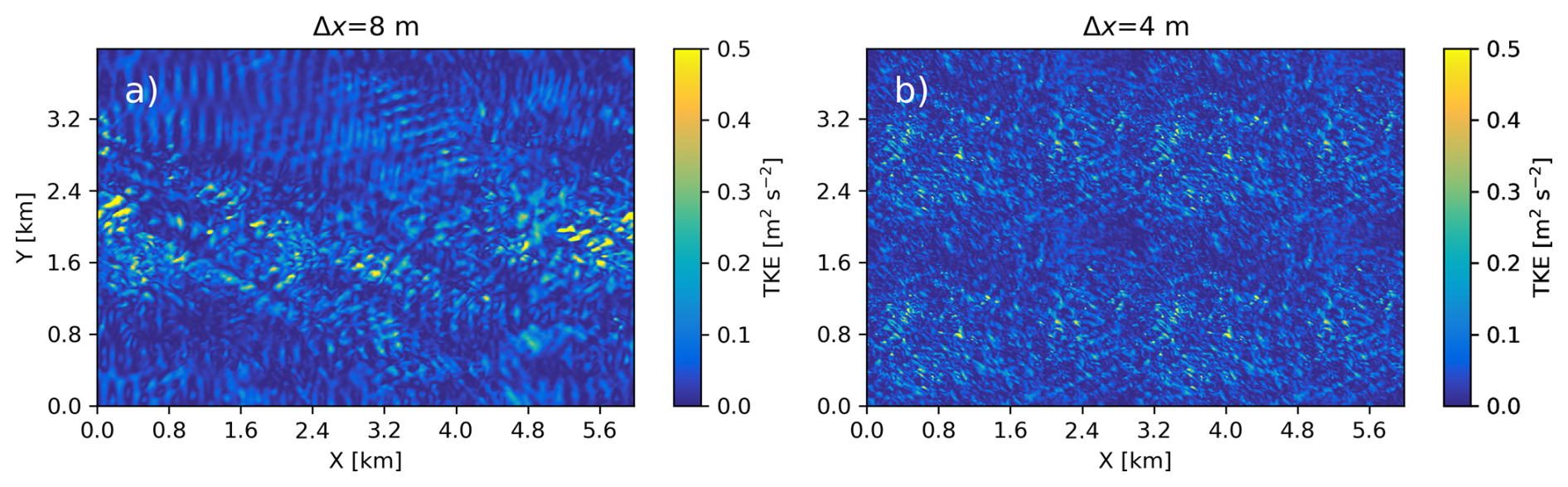
Figure A1 Instantaneous plan view of TKE at the beginning of the analysis period at 50 m above the ground for the strongly stable regime using the TKE-1.5 closure at (a) 8 m horizontal grid spacing and (b) 4 m horizontal grid spacing. Note that the domain is tiled in (b) for visualization purposes as the simulated domain for the 4 m grid spacing case is half of the length and width compared to the 8 m grid spacing case. Evident in (a) are wave-like patterns that are numerical artifacts.

For all the resolutions and both turbulence closures, the percentage of resolved heat flux to total heat flux decreases with increasing stratification. This indicates that runaway cooling does not occur in any of the simulations (Jiménez and Cuxart, 2005; Zhou and Chow, 2011). At 8 m resolution and for the strongly stable case, the DRM closure resolves over 30 % of the heat flux, while the TKE-1.5 closure resolves just 11 %. Even though the two closures have comparable average surface heat flux values during the analysis period (−0.041 K m s⁻¹ for the TKE-1.5 closure and −0.040 K m s⁻¹ for the DRM closure), the quality of resolved turbulence is substantially different. The DRM closure resolves nearly 3 times as much turbulence on this grid for the strongly stable regime compared to the TKE-1.5 closure and, as a result, simulates more realistic turbulence. For the weakly stable regime, the DRM and TKE-1.5 closures perform comparably. When the grid resolution is increased, both closures resolve more of the heat flux but with greater improvement for the TKE-1.5 closure vs. the DRM closure. The TKE-1.5 closure is improved significantly for the strongly stable case when the grid spacing decreases to 4 m and resolves a similar but slightly lower percentage of the heat flux at 26 % vs 32 % for the DRM closure. Additionally, for the weakly stable case (Fig. 3a), the TKE-1.5 closure resolves more heat flux. This is because, for the DRM closure, the effect of incorporating explicit filtering increases the total SFS modeled stress, and thus the resolved stress must decrease accordingly. This is a known feature of the DRM which helps decrease numerical error near the filter cutoff. For the strongly stable regime (Fig. 3c), much of the heat flux is modeled so the effect of the RSFS term on the resolved field is less pronounced. Similar results to the $q/Q$ ratios hold for other turbulence quantities such as turbulent kinetic energy (TKE) or momentum flux (not shown).

Table A1 Vertically integrated resolved heat flux q over total (resolved + subfilter) heat flux Q and computational cost factor for the TKE-1.5 and DRM closures at various horizontal grid spacings. The computational cost factor is the increase in computation cost relative to the 8 m, weakly stable simulation using the TKE-1.5 closure.

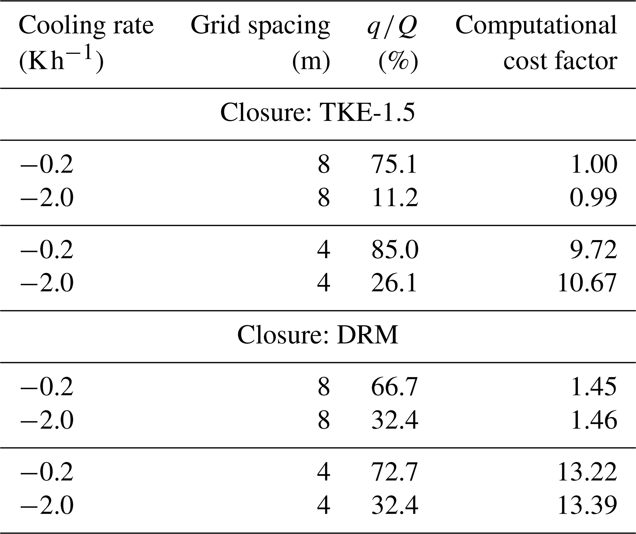
The computational cost factor in Table A1 is calculated by comparing the wall-clock time each simulation takes relative to the 8 m, weakly stable simulation using the TKE-1.5 closure. The cost factor inherently accounts for the decrease in time step required when the grid resolution is increased. The time steps used are 0.5 and 0.2 s for the 8 and 4 m grid spacing simulations, respectively. The same number of grid points is used for the 4 m configuration due to computational expense, as 4 times the number of grid points would be needed to keep the domain size consistent. The vertical resolutions for the 8 and 4 m configurations are identical (as defined previously). The cost factor is also adjusted to compare a constant physical domain size when the grid resolution is increased, which results in a default factor of 4 in the cost calculation for the 4 m grid spacing simulations compared to the 8 m case. For example, on 400 processors, the 8 m grid spacing TKE-1.5 weakly stable simulation takes 4.1 h of real time for every 1 h of simulation time, while the configuration with 4 m grid spacing takes 10.0 h with the same number of grid points. When the factor of 4 is included to compare a constant physical domain size, the 4 m grid spacing simulation would take 40.2 h, which results in a computational cost factor of 9.72. Using the DRM closure at the same resolution as the TKE-1.5 closure is 1.45 times the computational cost. At the same resolution, the TKE-1.5 closure outperforms the DRM closure with respect to $q/Q$ for the weakly stable regime at less computational cost. However, the DRM closure outperforms the TKE-1.5 closure for the strongly stable case even at the coarser 8 m grid spacing compared to the 4 m TKE-1.5 configuration, although the differences in $q/Q$ are minor. For the strongly stable case, the TKE-1.5 closure at 4 m resolution will resolve similar levels of turbulence at 7.3 times ($\mathrm{10.67}/\mathrm{1.46}$ from Table A1) the computational cost compared to the DRM closure at 8 m resolution. As a result, the DRM closure is better suited and more computationally efficient than the TKE-1.5 closure for simulating strongly stable boundary layers at coarser grid spacings. There are additional benefits of the DRM closure in the representation of intermittent turbulence, as further described in the main text of this paper. Note that there are some differences in the computational cost factor for the same resolution and closure, but with different cooling rates because the cost can vary slightly in the MOST iterative procedure at the surface.

Lastly, plan views of TKE at 50 m above the ground (70 % of the boundary layer height) for the TKE-1.5 closure at 8 and 4 m grid spacings are shown in Fig. A1. The TKE signals are processed in a similar manner to those shown for the DRM closure in Fig. 8. At 8 m grid spacing, the TKE signal displays wave-like patterns that are numerical artifacts due to unphysical temperature gradients. When using the TKE-1.5 closure, only by reducing the horizontal grid spacing from 8 to 4 m does the turbulence exhibit similar characteristics to the DRM closure at a horizontal grid spacing of 8 m. This is expected for the strongly stable regime as using the DRM closure at 8 m horizontal grid spacing resolves a similar level of heat flux (a proxy for TKE) to that when using the TKE-1.5 closure at 4 m horizontal grid spacing (Table A1).

Appendix B: Shear and buoyancy in the strongly stable regime

The gradient Richardson number further demonstrates the competition between shear generation and buoyancy suppression of turbulence in the strongly stable regime. We calculate the gradient Richardson number, Ri, as follows:

$$\begin{array}{}\text{(B1)}& {\displaystyle }{\displaystyle }\mathit{Ri}={\displaystyle \frac{N^{\mathrm{2}}}{S^{\mathrm{2}}}}={\displaystyle \frac{\frac{g}{\mathit{\theta }}\frac{\partial \mathit{\theta }}{\partial z}}{{\left(\frac{\partial u}{\partial z}\right)}^{\mathrm{2}}+{\left(\frac{\partial v}{\partial z}\right)}^{\mathrm{2}}}},\end{array}$$

where N² is the squared Brunt–Väisälä frequency (buoyancy), and S² is the squared vertical shear.

At the virtual tower 5D upwind of the wind farm, the gradient Richardson number profile as a function of height during the analysis period is shown in Fig. B1a. The colormap in Fig. B1a is chosen to emphasize a critical Richardson number of 0.25 (Stull, 1988). Above Ri=0.25, stratification dominates, and turbulence is suppressed by buoyancy. At a height of 50 m, the flow intermittently crosses the 0.25 threshold, as shown in Fig. B1b, illustrating the balance between buoyancy and shear.

Furthermore, a 1 h time average of shear, buoyancy, and the gradient Richardson number during the analysis period reveals that at 50 m above the ground, Ri is approximately 0.25. This finding complements the method in Sect. 3.2 in which we demonstrate the lowest intermittency fraction at a height of 50 m.

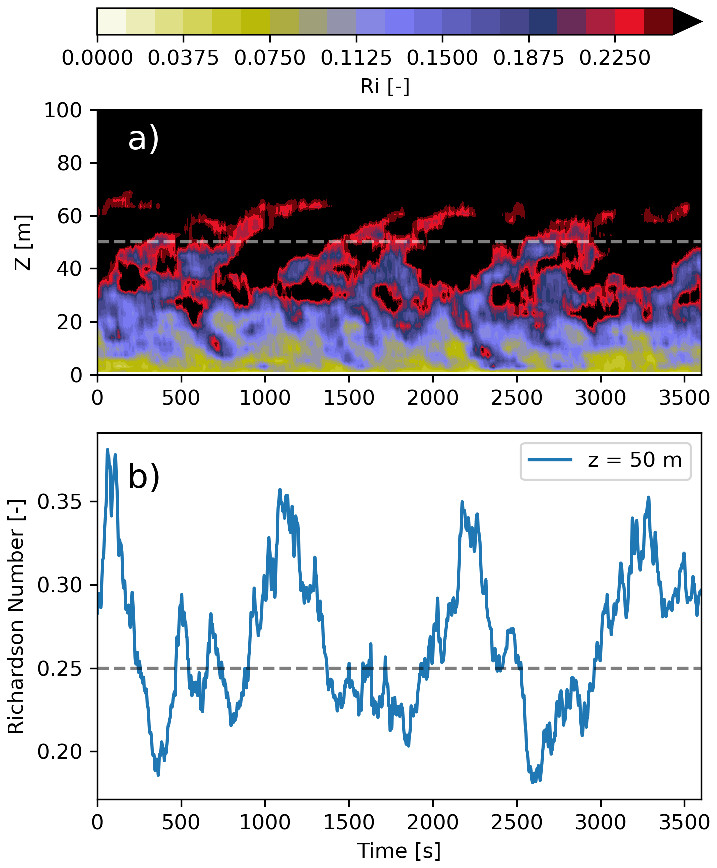
Figure B1 (a) Time–height contour of the gradient Richardson number (Ri) at 5D upwind of the wind farm on the inner domain during the analysis period emphasizing the critical Richardson number value of 0.25. (b) Time series of Ri at z=50 m with a dashed line at Ri=0.25 corresponding to the critical Richardson number.

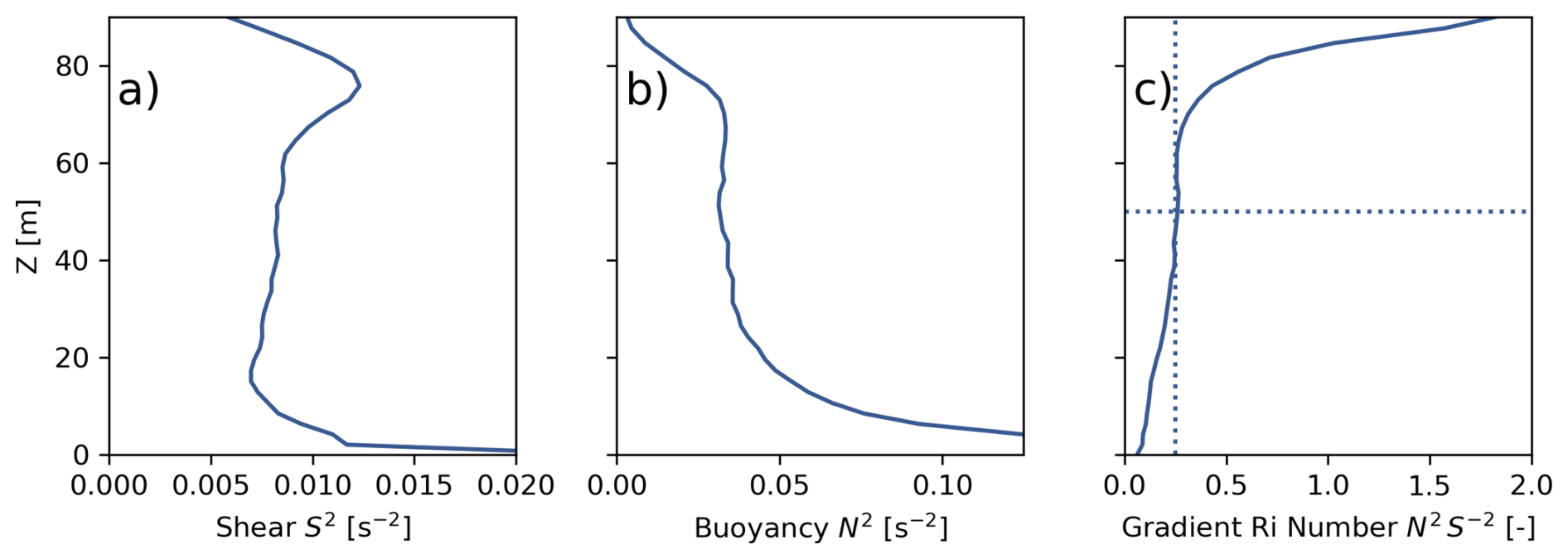
Figure B2 1 h time-averaged vertical profiles of (a) shear, (b) buoyancy, and (c) Ri during the analysis period. The dotted lines in (c) correspond to the critical Richardson number of 0.25 and a height of 50 m.