Calibration and validation of an engineering model for vortex-induced vibration prediction in wind turbine towers

The prediction of vortex-induced vibrations (VIV) caused by vortex shedding downstream of wind turbine towers is a complex and challenging engineering problem for wind turbine manufacturers. These vibrations typically occur when the turbine is in parked or idling mode or during the installation and commissioning phases. The paper reviews the current engineering framework for predicting VIV in wind turbine towers, with a focus on models that can be integrated into comprehensive aeroelastic design tools. It further explores the application of the Hartlen–Currie lift-oscillator model as a predictive tool for VIV in tower structures. In the paper, the free parameters of the Hartlen–Currie model are properly calibrated versus experimental results for rigid elastically mounted, untapered cylinders with the aim to capture the vibration amplitudes in the occurrence of lock-in events and the wind velocity at which maximum vibration amplitude is obtained. Once calibrated, the model is applied to simulate VIV in an elastic cantilevered cylinder. The results for both simply supported and cantilever configurations are then compared with experimental measurements and predictions from other widely used engineering models in the literature. The governing equations are expressed in a non-dimensional form to facilitate the calibration of the model's defining parameters. Comparisons with wind tunnel measurements show that the proposed model is capable of successfully predicting the maximum VIV vibration amplitudes and the frequency at which these occur.

1 Introduction

Vortex-induced vibrations (VIV) in wind turbine towers present a well-known challenge for wind turbine manufacturers (Veers et al., 2023). Numerous cases of excessive and often “unexpected” vibrations have been reported during the installation and commissioning phases – prior to electrification – as well as when turbines are parked or idling at low speeds. These vibrations are frequently attributed to fluctuating wind loads acting on the cylindrical tower, resulting from vortex shedding in its wake. It is noted that in some cases, vortex shedding originating from the blades can also induce unsteady aerodynamic loads and lead to VIV in the wind turbine structure (Horcas et al., 2022; Zou et al., 2015), but such vibrations are not within the scope of the present study. During VIV, substantial vibration amplitudes can develop within seconds across various components of the wind turbine, ultimately leading to limit cycle oscillations.

When the vortex shedding frequency approaches a natural frequency of a tower mode, a dynamic interaction occurs between the unsteady flow and the tower's elastic response – known as lock-in. The lock-in phenomenon is experienced by the turbine as a synchronization between its structural vibration frequency and the periodic aerodynamic excitation caused by the flow around the tower. VIV due to tower vortex shedding can occur under several conditions: (a) on the bare tower, before the rotor–nacelle assembly (RNA) is installed, (b) on partially assembled RNAs – with none, one, or two blades mounted, or (c) on the fully assembled turbine when the rotor is parked or rotating slowly in idling mode. It is important to note that tower vortex shedding can occur under all inflow conditions. However, during normal operation, rotor rotation enhances wake mixing, thereby disrupting coherent vortex structures and mitigating VIV.

For typical onshore and offshore wind turbines, once the rotor–nacelle assembly (RNA) is installed, the vortex shedding frequency of the tower often aligns with the first bending mode frequency of the structure at low to moderate wind speeds, typically in the range of 5–15 m s⁻¹. In contrast, when the RNA is not yet installed, the lock-in phenomenon tends to occur at higher wind speeds. In addition, onshore wind turbine manufacturers sometimes modify tower designs – particularly in terms of height and diameter – to better harness site-specific wind resources. For example, taller towers are often used at low-wind sites to access stronger wind flows at higher altitudes. In such cases, where towers can be up to 50% taller than standard configurations, the vortex shedding frequency may approach the second bending mode frequency of the tower, typically at wind speeds between 15–20 m s⁻¹. In both scenarios – whether due to the absence of the RNA or the use of tall towers – the elevated lock-in wind speeds result in larger aerodynamic excitation forces, which in turn cause more severe structural vibrations. A common feature in all these cases is that during lock-in, high-amplitude oscillations develop in the crossflow direction. In the case of the standalone tower, this is the direction with the lowest aerodynamic damping, as the damping of the longitudinal direction is substantially enhanced by the action of the tower drag force. The situation is slightly different in the case the RNA is installed, because the aerodynamic damping of both tower vibration directions is affected by the aerodynamic loading of the rotor, which depends on the pitch setting of the blades. In parked or idling operation, the rotor-induced damping is relatively small in both directions (Wang et al., 2017). As a result of the crossflow vibrations of the tower, fatigue damage is greatly accelerated, which potentially compromises the structural integrity of the wind turbine.

The prediction of wind turbine loads and vibration amplitudes during tower lock-in events primarily relies on the engineering framework established by the Eurocode standard (European Committee for Standardization (CEN), 2005; Manolas et al., 2022). According to this standard, the effects of vibrations induced by vortex shedding are represented as a periodic inertial force distribution along the height of the tower, acting perpendicular to the wind direction. This force is dependent on the tower's linear mass distribution, the frequency and mode shape of the excited structural mode, and the maximum vibration displacement amplitude, which can be determined using two alternative approaches provided in the Eurocode standard.

Engineering models in the literature are commonly classified according to how they represent the fluid forcing term, which in turn determines the degrees of freedom in the mathematical formulation (Fernandez-Aldama et al., 2024). In this work, we specifically distinguish between models based on whether they incorporate an explicit oscillator equation for the lift force.

A first class of alternative engineering models explored in the literature incorporates additional nonlinear aeroelastic force components into the sinusoidally varying lift force induced by vortex shedding around the cylindrical tower. These additional terms typically include a component in phase with the structural motion (aerodynamic stiffness) and/or a nonlinear component in phase with the motion velocity (aerodynamic damping). For a rigid elastically supported cylinder, such models are commonly expressed as single-equation formulations, where the nonlinear stiffness and/or damping forces are introduced as external excitations into the one-degree-of-freedom dynamic motion equation. Representative models of this type include those proposed in the literature (Basu and Vickery, 1983; Magnus et al., 2013; Scanlan, 1981). Although the aforementioned models can effectively predict the maximum vibration amplitude occurring during lock-in, they are unable to provide detailed information of the distribution of the self-excitation power within the lock-in region if constant values of the defining parameters of the model are considered. An improvement to the above shortcoming has been suggested in Kurniawati et al. (2025) and Livanos et al. (2024) by providing an experimentally calibrated map of the variation in the model's defining parameter as a function of the wind speed and the response amplitude. A critical review of the above models can be found in Lupi et al. (2018). In the above reference, prediction improvements are proposed for one-equation models, based on the results from wind tunnel experiments on a rigid cylinder undergoing imposed periodic motions.

A second class of engineering models investigated in the literature involves representing the aerodynamic excitation – specifically the lift force – through the solution of a second-order oscillator equation. A representative example of this type is the Hartlen and Currie model (Hartlen and Currie, 1970). For a rigid elastically supported cylinder, these models are formulated as coupled systems of two equations (and thus two state variables): the first is the structural dynamic equation of motion, and the second is the oscillator equation that governs the evolution of the lift force. The primary advantage of this class of models is that, even for constant values for its defining parameters, in addition to predicting the maximum vibration amplitude during lock-in, they are also capable of capturing the distribution profile of vibration amplitudes and response frequencies as a function of wind velocity within the lock-in region.

In the present study, a newly calibrated VIV model based on the Hartlen–Currie lift-oscillator equation is proposed, with the aim of serving as a predictive tool for wind turbine tower lock-in events that can be readily integrated into comprehensive, state-of-the-art aeroelastic design frameworks. The constants of the oscillator equation are identified through an optimization procedure designed to accurately reproduce the maximum oscillation amplitude of rigid elastically supported, untapered cylinders at the dimensionless wind velocity where this peak amplitude occurs. Subsequently, model constants and variations are introduced across the full range of dimensionless wind velocities to enable the model to reasonably capture the overall amplitude profile within the lock-in region. Target values for the maximum amplitude and corresponding dimensionless wind velocity are derived from two wind tunnel experiments (Belloli et al., 2012; Feng, 1968) conducted on rigid elastically supported cylinders with different Scruton numbers.

The calibrated oscillator equation is then integrated into NTUA's in-house multibody aeroelastic code, hGAST (Bagherpour et al., 2018; Manolas, 2016; Manolas et al., 2020; Panteli et al., 2022; Riziotis and Voutsinas, 1997), for the prediction of wind turbine tower loads and vibrations in elastic cantilevered cylinders. The lift equation is used to compute the lift force distribution along the correlation length, defined according to the Eurocode, for a cylindrical untapered wind turbine tower. Model predictions are validated against wind tunnel measurements (Lupi et al., 2021) of vibration amplitudes for an cylindrical untapered tower with a clamped base and a free top end, undergoing vortex-induced vibrations (VIV) at the natural frequency of its first bending mode. The results show that the model (calibrated based on measurements on rigid elastically mounted cylinders) successfully captures the maximum vibration amplitude and the maximum response amplitude wind speed at lock-in. To accurately estimate the range of wind velocities over which lock-in occurs, across a range of Scruton (Sc) numbers, the model needs further calibration based on observations from experimental data of clamped vibrating cylinders in their bending modes. It should be noted that vortex-induced vibrations in higher-order modes (second tower bending mode), as well as the influence of ambient turbulence on the development of the lock-in phenomenon, are not addressed in the present study and are identified as subjects for future research.

The paper is organized as follows. In Sect. 2, first, the lift-oscillator model and its parameter calibration procedure are introduced (Sect. 2.1). Next, the calibrated model's performance is assessed against state-of-the-art semi-empirical tools for vortex-induced vibration (VIV) prediction (Sect. 2.2); the integration of the lift-oscillator model into the existing multi-body solver is then described (Sect. 2.3). In Sect. 3, a comparison between the model predictions and experimental measurements on cantilever flexible cylinder are presented, whereas Sect. 4 provides the conclusions of the present work.

2 Methodology

The present work is structured into the following methodological steps:

• a.

  The two constants of the Hartlen–Currie lift-oscillator model are calibrated using data from two wind tunnel experiments conducted on rigid elastically mounted, untapered cylinders subjected to crossflow vortex-induced vibrations (VIV). The calibration aims at determining the constant values that yield the target maximum oscillation amplitude at the specific dimensionless velocity where this amplitude occurs within the lock-in region, and across different values of the Sc number. This is achieved through an optimization process using the COBYLA algorithm, as implemented in the “scipy.optimize” module of the SciPy library (Virtanen et al., 2020). For dimensionless velocities other than the one corresponding to the peak amplitude, a simplified parameter identification approach is employed by assuming a linear decay of the parameters from their values at maximum resonance. This follows the reasoning of Tamura (2020), who argues that parameter selection should not rely solely on curve fitting but must also respect the physical characteristics of the phenomenon.

• b.

  The calibrated lift-oscillator model is then integrated within the in-house multibody finite element method (FEM) structural solver, hGAST. In this framework, the 3D cantilever cylinder is modelled as a Timoshenko beam, offering a simplified yet robust aeroelastic model for predicting VIV on cantilevered wind turbine tower structures. The Hartlen–Currie lift equation is solved at each time step for every finite element, in strong coupling with the structural beam equations – an iterative procedure is followed until both the aerodynamic and structural solutions converge. The aerodynamic lift force predicted by the model is distributed along the height of the tower and applied as an external load to the corresponding finite elements. The correlation length, defined as the portion of the tower over which the aerodynamic loads are applied, is incorporated following Eurocode guidelines and depends on the maximum oscillation amplitude. Beyond this correlation length, the external forcing is reduced to zero.

2.1 The Hartlen–Currie two-equation lift-oscillator model

In the following subsections the Hartlen–Currie two-equation lift-oscillator model is presented along with the calibration procedure for the determination of the constants of the model.

2.1.1 Equations of the model of the rigid elastically mounted cylinder

In the Hartlen–Currie two-degrees-of-freedom (DOF) model, the second-order in time differential equation of motion for a rigid elastically supported cylinder in the direction perpendicular to the inflow velocity (the motion is denoted by the displacement y in Fig. 1) is coupled with a second-order, nonlinear differential equation that governs the dynamic lift coefficient C_L:

$$\begin{array}{}\text{(1)}& {\displaystyle }& {\displaystyle }m\ddot{y}+c\dot{y}+ky=C_{\mathrm{L}}{\displaystyle \frac{\mathit{\rho }}{\mathrm{2}}}{U}^{\mathrm{2}}Dl,\text{(2)}& {\displaystyle }& {\displaystyle }{\ddot{C}}_{\mathrm{L}}-G\left(-\left({\displaystyle \frac{\mathrm{4}}{\mathrm{3}}}\right){\left({\displaystyle \frac{{\dot{C}}_{\mathrm{L}}}{{\mathit{\omega }}_{\mathrm{s}}}}\right)}^{\mathrm{2}}+C_{\mathrm{L}\mathrm{0}}\right){\dot{C}}_{\mathrm{L}}+{\mathit{\omega }}_{\mathrm{s}}^{\mathrm{2}}{C}_{\mathrm{L}}=-H\dot{y}.\end{array}$$

Figure 1 Elastically supported cylinder.

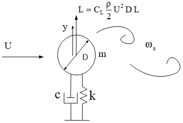
In Eq. (1), m, k and c are the mass of the cylinder and the spring and damping coefficients of its elastic support, D is diameter and l the length of the cylinder, and U is the inflow velocity and ρ the density of the fluid. The constants G and H in Eq. (2) are free parameters of the model that need to be provided by the user of the model. Parameter G calibrates the aerodynamic damping ($-G{C}_{\mathrm{L}\mathrm{0}}{\dot{C}}_{\mathrm{L}}$), which is always negative for positive values of G. The non-linear factor $G(\mathrm{4}/\mathrm{3})({{\dot{C}}_{\mathrm{L}}}^{\mathrm{2}}/{\mathit{\omega }}_{\mathrm{s}}^{\mathrm{2}})$ ensures the self limiting nature of the response provided by the equation. Parameter H represents the feedback of the structural motion to the lift coefficient. In the model by Hartlen and Currie, the forcing term is taken to vary linearly with the structural velocity. The factor $\mathrm{4}/\mathrm{3}$ emerges through the requirement that in the case of no external forcing (H=0), the work done by the damping terms should be zero. This also requires that the lift coefficient is a pure harmonic function. Furthermore, ω_s=2πf_s in Eq. (2) is the shedding angular frequency (and f_s the corresponding frequency) of the rigid cylinder (corresponding to the shedding Strouhal number St), and C_L0 is the standard deviation of the lift coefficient (due to vortex shedding) of the rigid cylinder case. Both St and C_L0 are obtained from experiments on rigid cylinders as functions of the Reynolds number (Re) (Facchinetti et al., 2004; Schewe, 1983).

Equations (1) and (2) can be expressed in non-dimensional form by introducing the non-dimensional displacement and time parameters η and τ respectively, defined as

$$\mathit{\eta }=y/D\mathit{\tau }=tU/D.$$

The non-dimensional Eqs. (1) and (2) are then written

$$\begin{array}{}\text{(3)}& {\displaystyle }{\mathit{\eta }}^{\prime \prime }+\left({\displaystyle \frac{\mathrm{4}}{m^{\ast }{U}^{\ast }\mathit{\pi }}}\mathit{Sc}\right){\mathit{\eta }}^{\prime }+\left({\displaystyle \frac{\mathrm{4}{\mathit{\pi }}^{\mathrm{2}}}{U^{\ast \mathrm{2}}}}\right)\mathit{\eta }={\displaystyle \frac{\mathrm{2}{C}_{\mathrm{L}}}{m^{\ast }\mathit{\pi }}},\text{(4)}& {\displaystyle }\begin{array}{rl}{C}_{\mathrm{L}}^{\prime \prime }& -\left({\displaystyle \frac{GD}{U}}\right)\left(-\left({\displaystyle \frac{\mathrm{4}}{\mathrm{3}}}\right){\displaystyle \frac{C_{\mathrm{L}}^{\prime \mathrm{2}}}{\mathrm{4}{\mathit{\pi }}^{\mathrm{2}}{\mathit{St}}^{\mathrm{2}}}}+C_{\mathrm{L}\mathrm{0}}\right)C_{\mathrm{L}}^{\prime }\\ & +\mathrm{4}{\mathit{\pi }}^{\mathrm{2}}{\mathit{St}}^{\mathrm{2}}{C}_{\mathrm{L}}=-\left({\displaystyle \frac{H{D}^{\mathrm{2}}}{U}}\right){\mathit{\eta }}^{\prime }.\end{array}\end{array}$$

In Eqs. (3) and (4), $(\cdot {)}^{\prime }=\frac{\mathrm{d}}{\mathrm{d}\mathit{\tau }}(\cdot )$, $m^{\ast }=\frac{\mathrm{4}{m}_{\text{eq}}}{\mathit{\pi }\mathit{\rho }{D}^{\mathrm{2}}}$ is the dimensionless mass ratio of the cylinder, $m_{\text{eq}}=m/l$ the linear mass of the cylinder, and $U^{\ast }=\frac{U}{f_{\mathrm{n}}D}$ is the dimensionless flow velocity, where $f_{\mathrm{n}}=({\mathit{\omega }}_{\mathrm{n}}/\mathrm{2}\mathit{\pi })=\sqrt{k/m}/\mathrm{2}\mathit{\pi }$ is the natural frequency of the elastic cylinder and $\mathit{Sc}=\frac{\mathrm{4}\mathit{\pi }{m}_{\text{eq}}\mathit{\zeta }}{\mathit{\rho }{D}^{\mathrm{2}}}$ is the dimensionless Scruton number, where ζ is the critical damping ratio given by $\mathrm{2}\mathit{\zeta }{\mathit{\omega }}_{\mathrm{n}}=c/m$ and $\mathit{St}=\frac{f_{\mathrm{s}}D}{U}$ is the shedding Strouhal number.

Notably, in Eq. (4), the coefficients $\frac{GD}{U}$ and $\left(\frac{H{D}^{\mathrm{2}}}{U}\right)$ can be replaced by two new constants G^′ and H^′, which remain unchanged for a given set of the dimensionless parameters m^∗, Sc, U^∗, and St, independent of the actual values of the dimensional parameters of the problem. The non-dimensional formulation of Eqs. (3) and (4) facilitates the calibration of the model's defining constants, since this process must be carried out only once for a specified set of dimensionless parameters.

It is noted that in the present study we chose to define G^′ and H^′ as follows:

$$\begin{array}{}\text{(5)}& {\displaystyle }& {\displaystyle }{G}^{\prime }={\displaystyle \frac{G}{{\mathit{\omega }}_{\mathrm{s}}}}={\displaystyle \frac{GD}{U}}\left({\displaystyle \frac{\mathrm{1}}{\mathrm{2}\mathit{\pi }\mathit{St}}}\right),\text{(6)}& {\displaystyle }& {\displaystyle }{H}^{\prime }={\displaystyle \frac{HD}{{\mathit{\omega }}_{\mathrm{s}}}}={\displaystyle \frac{H{D}^{\mathrm{2}}}{U}}\left({\displaystyle \frac{\mathrm{1}}{\mathrm{2}\mathit{\pi }\mathit{St}}}\right).\end{array}$$

It is also worth noting that, for a typical vortex-shedding Strouhal number of 0.2 in the subcritical regime, the dimensionless velocity at which the vortex-shedding frequency of the rigid cylinder matches the natural frequency of the elastically mounted cylinder is U^∗ = 5.

2.1.2 Model constants' calibration procedure

The constants G^′ and H^′of the Hartlen–Currie lift-oscillator model are calibrated using data from wind tunnel experiments conducted on rigid untapered, elastically mounted cylinders subjected to crossflow vortex-induced vibrations (VIV). In the existing literature, the calibration of van der Pol or Rayleigh-type oscillators typically assumes constant parameter values across the lock-in range, with these parameters optimized based on relevant experimental data (Facchinetti et al., 2004; Farshidianfar and Dolatabadi, 2013). In the present study, we employ the Hartlen–Currie model with variable calibration parameters, as described in this section, in order to more accurately capture the VIV response over a range of critical velocities.

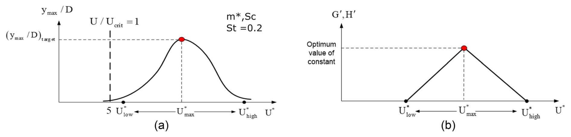
Figure 2 Schematic representation of the calibration process for the constants $G^{\prime },H^{\prime }$. Calibration is carried out for experimental $y_{max}/D$ at $U_{max}^{\ast }$ (a). Within the critical range the parameters are assumed to decrease linearly from their calibrated values (b).

The calibration procedure is illustrated in Fig. 2. Experimental studies provide data on the variation in the maximum vibration amplitude y_max with respect to U^∗, for different values of the Scruton number. In most cases, experiments are carried out for only one or a limited range of m^∗ values. As shown in Fig. 2, the ultimate maximum amplitude typically occurs at U^∗ values greater than those for which the natural frequency of the elastically mounted cylinder equals the shedding frequency of the rigid cylinder (as noted above, this corresponds to U^∗ = 5 for St = 0.2) or at wind velocities exceeding the critical value ($U/U_{\text{crit}}$ > 1), where U_crit is defined by the following expression:

$$\mathit{St}=\mathrm{0.2}={\displaystyle \frac{f_{\mathrm{n}}D}{U_{\text{crit}}}}.$$

For each available experimental dataset of m^∗, Sc, and St, an optimization loop is executed using the COBYLA method, as implemented in the Python SciPy package (Virtanen et al., 2020), to determine the optimal values of the constants G^′ and H^′ that yield the target peak amplitude y_max at the corresponding measured $U_{max}^{\ast }$. The differential Eqs. (3) and (4) are numerically integrated in time until resonant oscillations build up. The objective of the optimization procedure is to minimize the difference between the oscillation amplitude obtained for a given pair of constants with the target amplitude. Numerical integration is performed using the implicit second-order Newmark method as implemented in Zou et al. (2015). Once the optimal G^′ and H^′ are determined for $U_{max}^{\ast }$, a simplified approach is applied to describe their variation for U^∗ values other than $U_{max}^{\ast }$. The lock-in region is assumed to lie within a specific U^∗ range $\left[U_{\text{low}}^{\ast }{U}_{\text{high}}^{\ast }\right]$ as indicated by experimental data (that is, the range of U^∗ over which y_max remains significant). It is then assumed that G^′ and H^′ (the values determined through the optimization loop) decrease linearly to zero from $U_{max}^{\ast }$ towards both $U_{\text{low}}^{\ast }$ and $U_{\text{high}}^{\ast }$ as shown in Fig. 2. By gradually reducing the parameters to zero, the model is gradually disabled, leading to less pronounced limit cycle oscillations. Outside the lock-in zone, setting the constants equal to zero reduces the equations to a harmonic oscillator. For the purposes of this VIV model we assume that limit cycle oscillations due to vortex shedding are negligible outside the lock-in range. Through the above procedure, a single set of optimal G^′ and H^′ values characterizes each combination of the dimensionless parameters governing the physical problem. This approach eliminates the need for complex optimization simulations across the entire lock-in range, while ensuring that the physical parameters of the problem (extent of lock-in range) are preserved.

In the following sections, the constants of the Hartlen–Currie model are optimized using two distinct experimental datasets for rigid untapered, elastically supported cylinders. For each experiment, optimization is carried out for a single m^∗ value, thereby not accounting for any changes in the mass ratio. However, the optimization covers a range of Sc values. It should also be noted that both experiments were conducted within the subcritical Reynolds number regime, where the Strouhal number of vortex shedding is approximately 0.2.

2.2 Model calibration results

Two experimental wind tunnel datasets on VIV of a rigid untapered, elastically supported cylinder are used to calibrate the parameters of the lift-oscillator equation. The first and more recent campaign is by Belloli et al. (2012). It was conducted at the POLIMI wind tunnel on a cylinder with diameter D = 0.2 m, aspect ratio $l/D=\mathrm{10}$, mass ratio $m^{\ast }=\mathrm{170}$, and at a nominal Re = 4.6 × 10⁴ (in the subcritical regime). The measured vortex shedding Strouhal number of the rigid cylinder at the above conditions was St=0.18 and a turbulence intensity of 2 %. Tests are conducted for three values of the Sc number, Sc = 1.00, 4.36, 6.67. The second and older test by Feng (1968) was conducted in the wind tunnel at the University of British Columbia on a cylinder with diameter D = 0.076 m, aspect ratio $l/D=\mathrm{9}$, mass ratio $m^{\ast }=\mathrm{248}$, and Re = 1 × 10${}^{\mathrm{4}}/$ 5 × 10⁴ (again in the subcritical regime). The measured vortex shedding Strouhal number was St=0.198, the turbulence intensity was 0.1 %, and the Sc number varied in the range $\mathit{Sc}=\mathrm{2.52}/\mathrm{7.92}$. Since the numerical model as employed does not implicitly take turbulence into account, calibration would ideally be carried out using experimental measurements of low ambient turbulence. Existing experimental data exhibit turbulent levels ranging from ∼ 0.1 %–2 %, which are deemed less than the typical values of ambient turbulence in anticipated field conditions.

Before proceeding with the calibration of the Hartlen Currie model, the capabilities of three commonly used in the existing literature models in predicting the maximum VIV amplitude are assessed. Measured data from the two tests discussed above are compared to the analytical model of Blevins (1977) and the one-equation models discussed in the introduction section, namely the models proposed by Scanlan (1981) and Ehsan and Scanlan (1990), as well as the Single Degree of Freedom Aerodynamic Damping Model (1DOF-ADM) (Lupi et al., 2018; Magnus et al., 2013). As evidenced in Fig. 3, the current state of the art provides reasonable maximum amplitude predictions. However, different models exhibit different levels of accuracy in different Sc number regimes. Figure 3a and b present the measured peak VIV amplitudes from the two experiments as functions of the Scruton number (Sc). In Fig. 3a, the experimental results of Feng (1968) and Belloli et al. (2012) are compared against the predictions of Eurocode Approach 2 and the Blevins one-equation model. The predictions of Eurocode Approach 2 (Appendix D) predict maximum oscillation amplitudes around ∼ $\mathrm{0.5}{y}_{max}/D$ for the experimental setups, although they tend to be conservative as Sc increases. In Fig. 3b, smooth logarithmic trend lines have been fitted through both experimental datasets, which are then compared with the predictions of two one-equation models by Scanlan and 1DOF-ADM. The governing equations of these models are provided in the Appendix along with a full list of symbols. The peak amplitudes obtained from the smooth trend lines are subsequently employed in the calibration procedure rather than the raw measurement data. This approach minimizes the influence of outliers in the experimental data, such as the anomaly observed in the Belloli test for Sc=4.36. A comparison of the two experimental datasets shows that the more recent measurements by Belloli et al. (2012) exhibit significantly larger oscillation amplitudes at Sc=4.36 but are in close agreement with Feng's results for higher Sc values (Sc>6). Comparison between model predictions and experimental data reveals that the Blevins model tends to slightly overpredict peak amplitudes at high Sc values (Sc>6), while considerably underpredicting them at low Sc values (Sc≈ 1). Regarding the one-equation models, the results indicate that Scanlan's model generally provides better agreement with measurements than the 1DOF-ADM. The latter offers reasonable peak amplitude predictions at high Sc values but underestimates amplitudes for Sc<3.

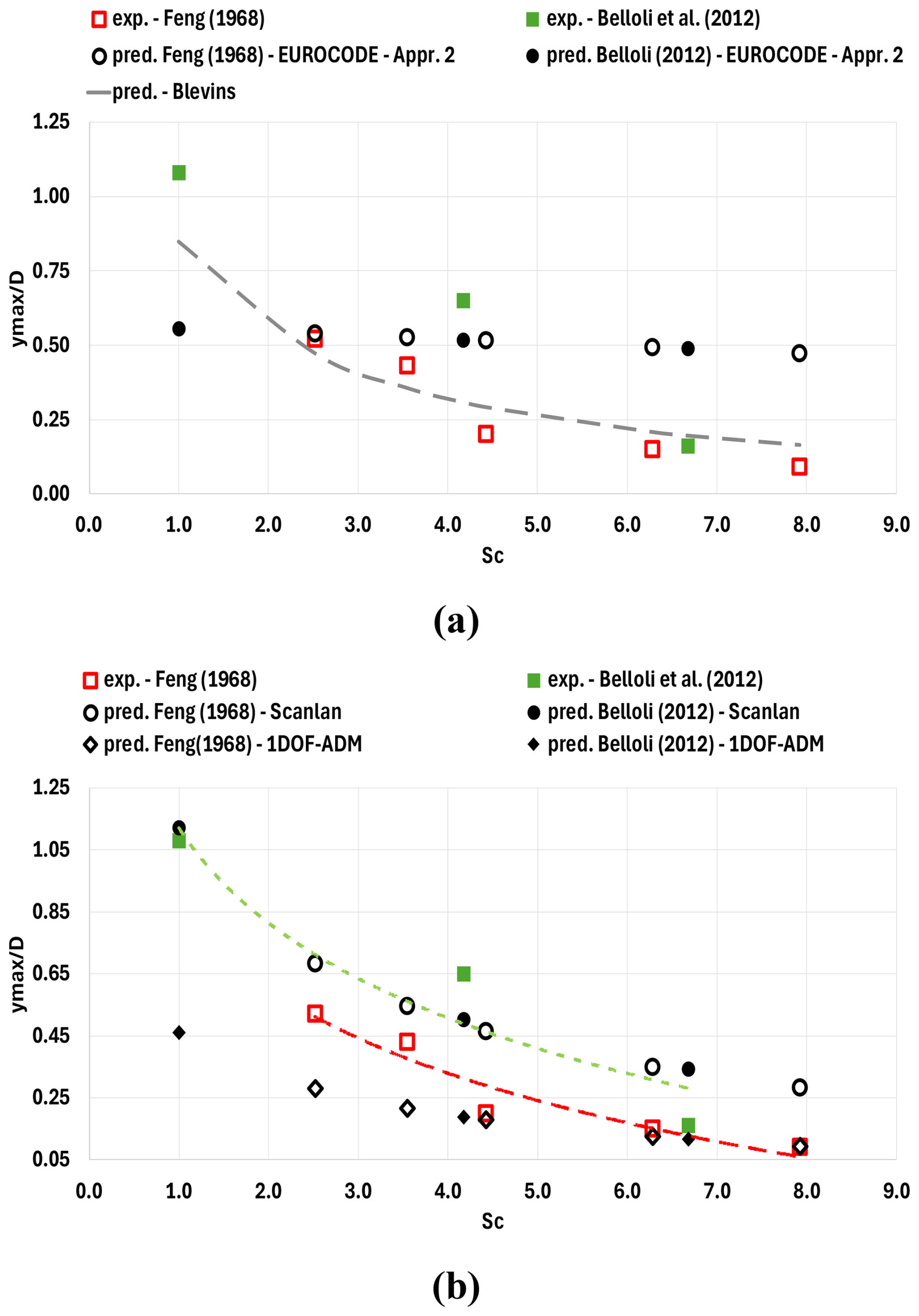
Figure 3 Maximum oscillation amplitude in VIV. Comparison of two wind tunnel tests results with different models from the literature.

In the following, the results of the calibration procedure for the constants of the Hartlen–Currie model are provided. The experimental measurements on which the calibration was based, alongside the calibrated model's predictions, are presented in Figs. 4 and  6. Since the parameters are assumed to vary linearly within the critical region, we consider the critical velocity range to lie in U\U_crit = 1–1.6, which is expressed using the reduced velocity U^∗. Since U^∗ depends on St and the two experiments report different values, the critical U^∗ ranges for each calibration dataset are different.

For the Belloli dataset, the range $[U_{\text{low}}^{\ast },U_{\text{high}}^{\ast }]$ within which the parameters G^′ and H^′ take non-zero values is defined as [5.5,9] based on examination of the measured data and the reported St, which is equal to 0.18. Although the experimental data show a decay of VIV below $U_{\text{high}}^{\ast }=\mathrm{9}$, this value is deemed high enough to allow the calibrating constants to dictate the zone width naturally, rather than imposing an overly restrictive a priori limit. In the optimization simulations C_L0 was taken equal to 0.3 (Schewe, 1983; Norberg, 2003), the amplitude value that corresponds to the subcritical regime of the Re number.

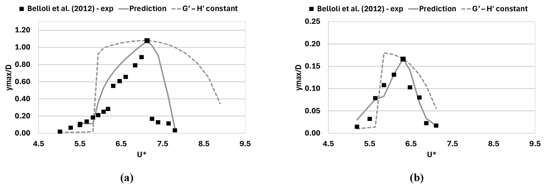
Figure 4 Oscillation amplitudes vs. U^∗. Calibration of the model constants with measurements from Belloli et al. (2012). Predictions correspond to varying and constant G^′ and H^′. Two Sc values are addressed: (a) Sc=1, (b) Sc=667. Mass ratio $m^{\ast }=\mathrm{170}$ and Re = 46 × 10⁴.

In Fig. 4, the amplitudes predicted by the newly calibrated model peak are compared to the measured data by Belloli et al. (2012). Given that the results of the proposed method rely heavily on the selection of the range $[U_{\text{low}}^{\ast },U_{\text{high}}^{\ast }]$, a simpler alternative of maintaining constant G^′ and H^′ values across the entire U^∗ range is also assessed. The constant values used are those obtained from the optimization run at $U_{max}^{\ast }$. For the high Sc number case (Sc = 6.67, representing high damping), both methods accurately capture the dimensionless velocity range of the lock-in and the peak oscillation amplitude during VIV. However, maintaining constant G^′ and H^′ values leads to a shift in $U_{max}^{\ast }$ towards the value that corresponds to $U/U_{\text{crit}}=\mathrm{1}$. In contrast, the method with varying G^′ and H^′ provides amplitude predictions that align better with the measurements. For the low Sc number case (Sc = 1.00, representing low damping), the constant G^′ and H^′ method slightly overpredicts the peak amplitude as well as the range of U^∗ for which oscillation amplitudes remain significant. Furthermore, a slight shift in high amplitudes towards lower U^∗ is again observed. On the other hand, the method with varying model constants (denoted as “Prediction” in the plots) provides a much closer agreement with measurements across the entire U^∗ range.

In Fig. 5, the dimensionless oscillation frequency for low and high Sc cases is presented. It is obtained by applying an FFT analysis to the displacement signal of the cylinder and comparing the resulting dominant response frequency with the natural frequency. The plateau of the frequency plot at $f/fn=\mathrm{1}$ signifies the occurrence of VIV, where the vortex shedding frequency locks in with the natural frequency, resulting in synchronized vortex shedding and structural vibrations. The extent of this plateau indicates the range of the lock-in, while departure from $f/fn=\mathrm{1}$ indicates the end of lock-in and the subsequent decay of oscillation amplitudes. The lock-in range is noticeably narrower for the higher Scruton number.

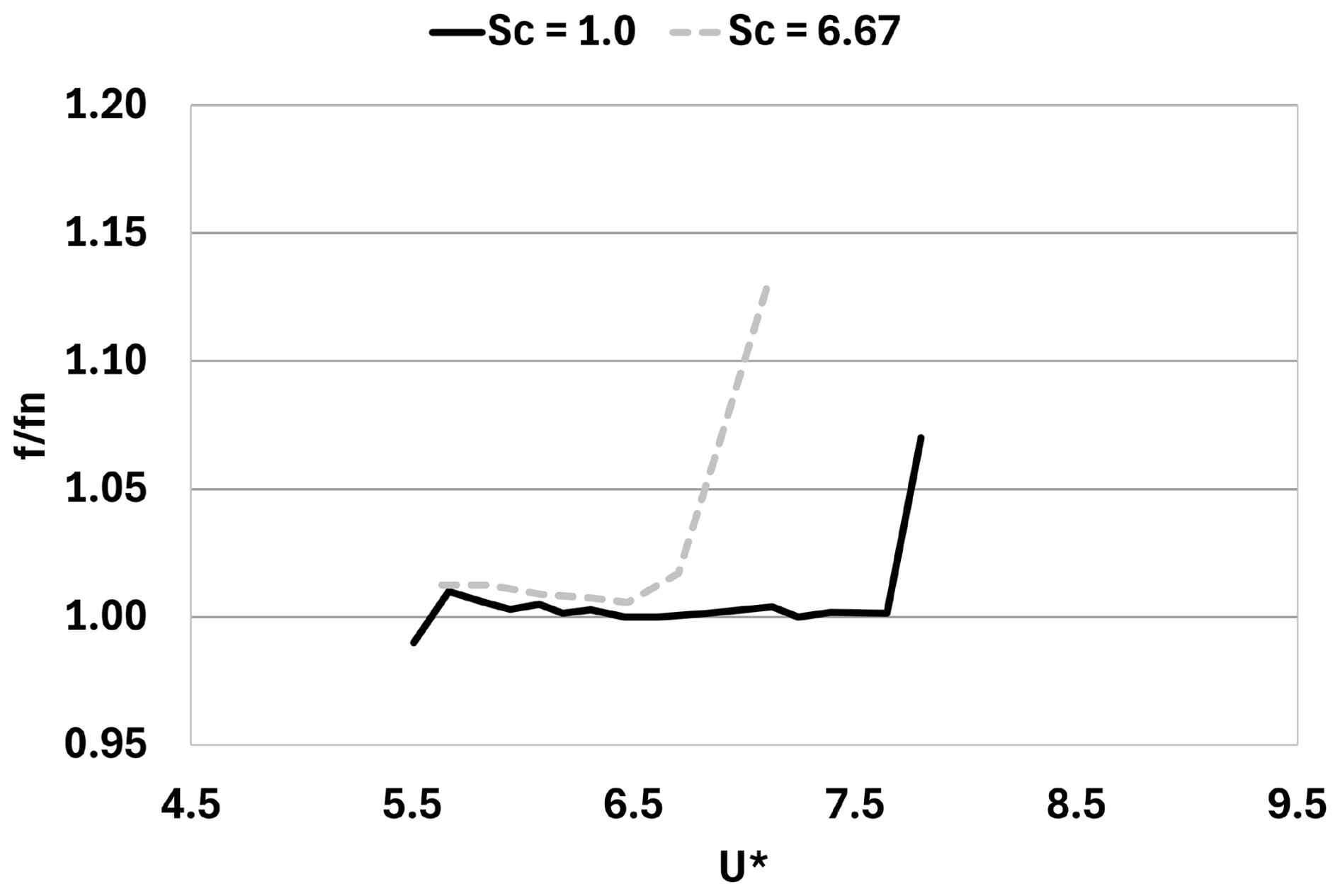
Figure 5 Frequency ratio across VIV zone for two Sc values obtained with the varying parameters approach. The plateau indicates resonance at the natural frequency, although the St shedding frequency varies. Frequencies are obtained by applying an FFT filter to the displacement of the body and obtaining the dominant frequency.

For the dataset of Feng (1968) the range $[U_{\text{low}}^{\ast },U_{\text{high}}^{\ast }]$ within which the parameters G^′ and H^′ take non-zero values is defined as [5,8] based on examination of the measured data and the reported St, which is equal to 0.198. As in the case of the first test, in the optimization simulations, C_L0 was taken equal to 0.3.

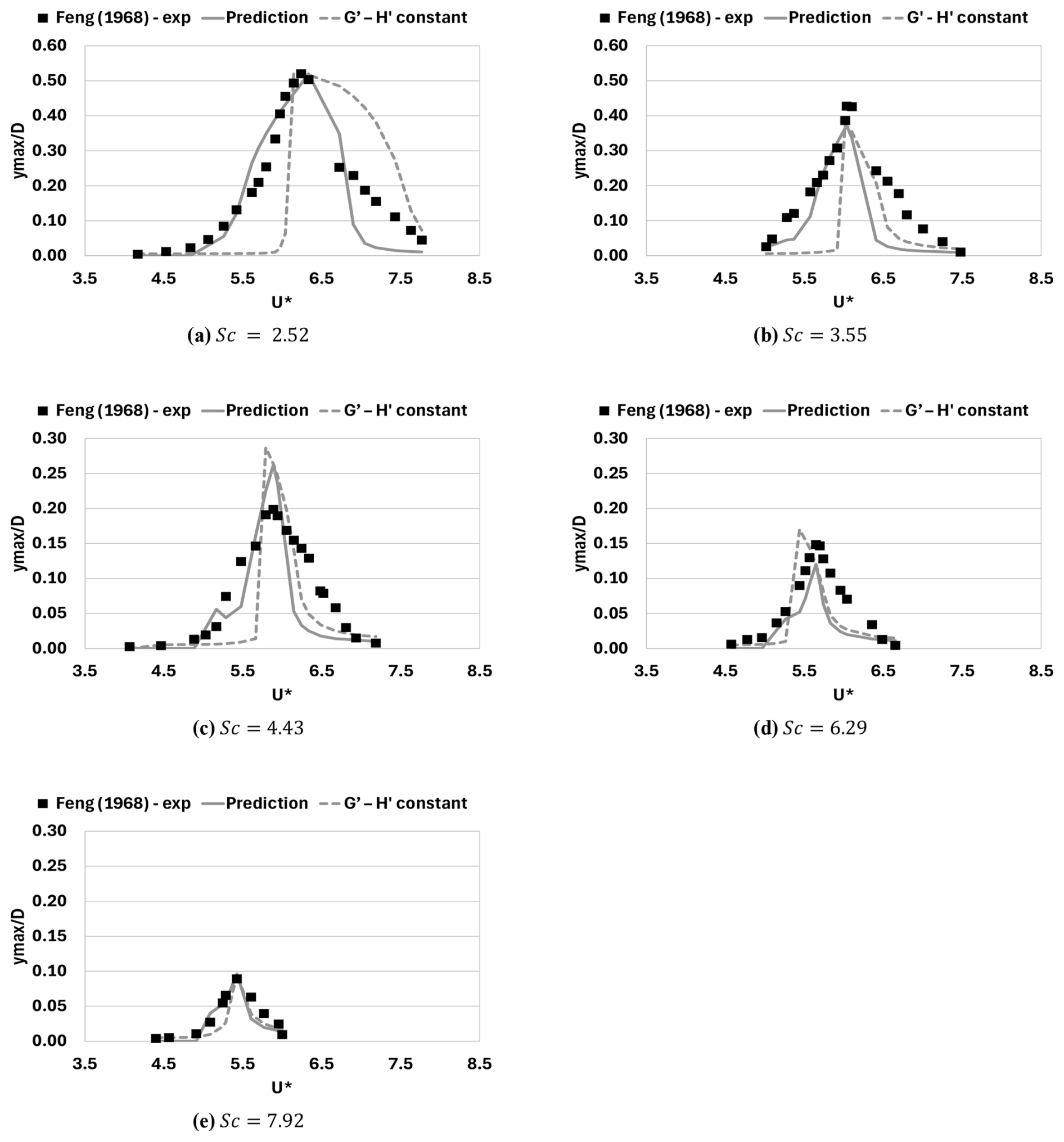
Figure 6 Oscillation amplitudes vs. U^∗. Calibration of the model constants with measurements from Feng (1968). Predictions correspond to varying and constant G and H. Scruton numbers range from 2.52 to 7.92. Mass ratio $m^{\ast }=\mathrm{248}$ and Re = 1 × 1${\mathrm{0}}^{\mathrm{4}}/\mathrm{5}\times {\mathrm{10}}^{\mathrm{4}}$.

As shown in Fig. 6, similar to the first test, the varying constants method provides reasonable predictions of the oscillation amplitudes within the lock-in region across all Sc numbers, exhibiting good agreement with the measurements. The inability to predict the ultimate maximum amplitude in certain cases (e.g. Sc=4.43 and 6.29) is attributed to the model constants being optimized based on the peak amplitudes derived from the smooth trend lines in Fig. 3, which sometimes deviate significantly from the measured values. Maintaining constant G and H exhibits a different behaviour for different Sc numbers. Overall, it predicts a narrower lock-in zone than the one predicted by the varying constants method and it also predicts fairly well the location of maximum resonance, with an exception at Sc=6.29.

The uncertainty in the model's behaviour when employed with constant parameters highlights a clear advantage of the varying parameters approach, in that it is less sensitive to the non-linearity of the model and the non-trivial effect of the magnitude of the calibrating parameters for different reduced velocities. Decreasing the parameters from their maximum value allows for a consistent capturing of both the maximum response conditions as well as the overall trend of the VIV response.

A comparison of the two tests, in terms of the variation in the peak amplitude in VIV as a function of the Sc number (Fig. 3), shows that they yield similar results, apart from the outlier at Sc = 4.43 in the POLIMI test, which has not been considered either for obtaining the logarithmic trend lines or for the calibration of the constants. However, a notable difference between the two experiments lies in the predicted U^∗ value at which maximum VIV response occurs. For all Sc numbers, the POLIMI test consistently provides higher $U_{max}^{\ast }$ values, although the two experiments are conducted in the same range of Re (O(10^∧4)). The main difference between the two experimental campaigns lies in the mass ratio of the cylinders. The POLIMI test was conducted at a lower mass ratio ($m^{\ast }=\mathrm{170}$) than Feng's test ($m^{\ast }=\mathrm{250}$), which could, to some extent, explain the difference. The differences between the measured responses of the two experiments and the resulting calibration values could also be attributed to different turbulence intensities in the flow. Feng (1968) reports low turbulence intensity values (∼ 0.1 %, whereas in the POLIMI setup the turbulence intensity is reported to be close to ∼ 2 % in a later reference (Belloli et al., 2015)). Despite the aforementioned difference, the constants obtained from the optimization runs for the two datasets exhibit similar trends, as shown in Fig. 7. The value of $G_{max}^{\prime }$ shows an almost linear decrease with increasing Sc, whereas the opposite behaviour is observed for the $H_{max}^{\prime }$ constant, which increases linearly with Sc. The parameter G^′ determines the amount of negative aerodynamic damping in Eq. (4), which controls the amplitudes of the VIV oscillations obtained. Therefore, $G_{max}^{\prime }$ is expected to exhibit a decreasing behaviour with increasing Sc. On the other hand, H^′ controls the magnitude of the excitation of Eq. (4). Therefore, a trade-off behaviour (decrease in $G_{max}^{\prime }$, followed by increase in $H_{max}^{\prime }$) between the two constants is anticipated as Sc tends to increase and the corresponding VIV amplitudes tend to decrease. In Fig. 7, alongside the optimal $G_{max}^{\prime }$ and $H_{max}^{\prime }$ values for the two tests, fitted trend lines are also presented. These lines will subsequently serve as envelope curves for determining appropriate constant values to be used in the cantilever tower analysis of Sect. 3.

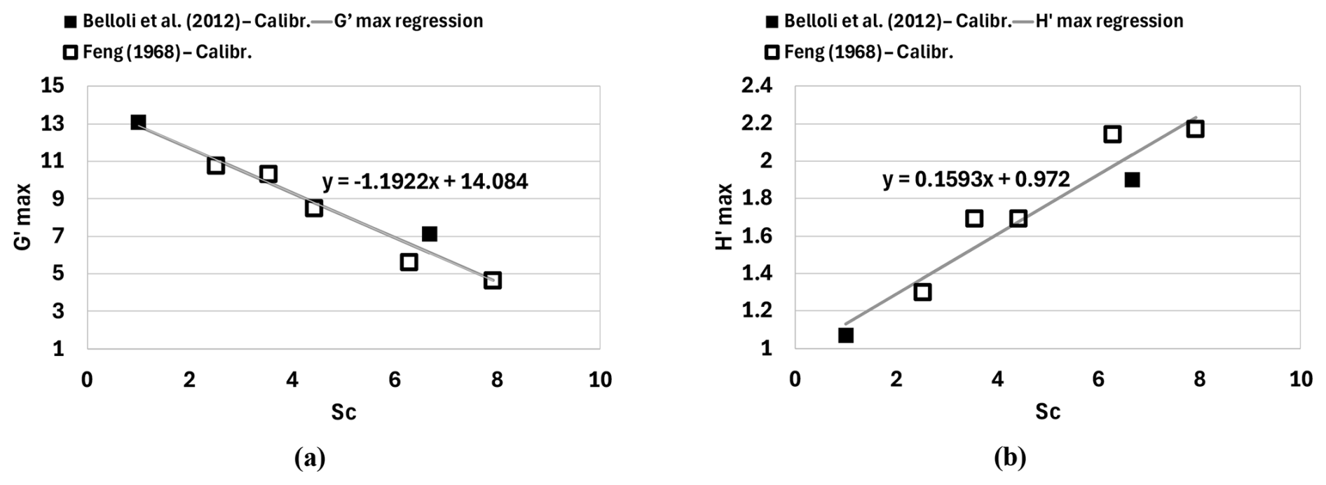
Figure 7 $G_{max}^{\prime }$ (a) and $H_{max}^{\prime }$ (b) across the range of Scruton numbers tested. Calibration with both experimental datasets yields very similar results and a common linear trend line is fitted.

2.3 Implementation of the Hartlen–Currie lift equation in hGAST

The lift-oscillator model presented and calibrated in Sects. 2.1 and 2.2 is integrated within the in-house multibody finite element method (FEM) hydro-servo-aero-elastic solver and stability analysis tool, hGAST (Manolas et al., 2020; Riziotis et al., 2008). hGAST models the full wind turbine as a multi-component dynamic system, having as components the blades, the drive train, and the tower. The components are assembled into the full configuration on the basis of the multibody formulation. It consists of considering each component separately from the others but is subjected to specific free-body kinematic and loading conditions, which are imposed at the connection points of the components. The multibody formulation is also extended to the level of the components (e.g. blades and tower), which can be divided into a number of sub-bodies connected to each other through similar kinematic and dynamic constraint conditions. In this way, geometric non-linearities related to large deflections are taken into account. All flexible components (blades, drive train, and tower) are modelled as Timoshenko beam structures subjected to bending, torsion, and tension and are approximated with the finite element method (FEM). An enhanced Blade Element Momentum Theory (BEMT) model approximates the aerodynamics of the rotor, taking into account mean inflow characteristics such as yaw, shear, veer, and inclination, as well as turbulent fluctuations. Viscous effects, unsteady airfoil aerodynamics, and dynamic stall are taken into account using the ONERA model. In the standard version of hGAST, the aerodynamic loading of the tower consists only of a steady drag force acting on every element of the tower in the direction of the incoming local flow (drag coefficient is defined as a function of the local Re number). The aerodynamic and structural dynamic problems are implicitly coupled (iteration are performed between the two problems until convergence of both is achieved). The integration of the system dynamic equations in time is performed using the Newmark second-order scheme.

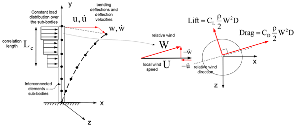
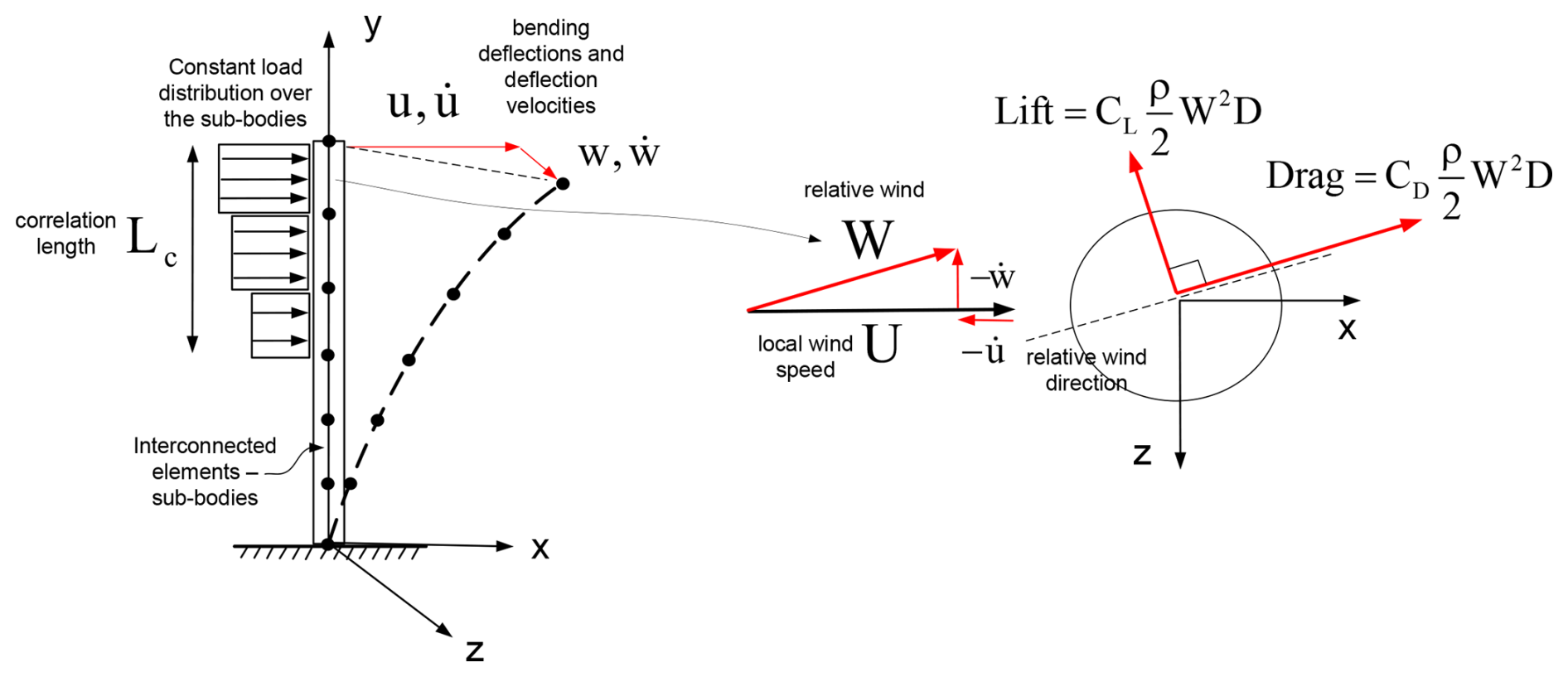
In the framework developed in the present work, the 3D cantilever cylinder is modelled as a collection of interconnected linear Timoshenko sub-bodies, offering a simplified yet robust aeroelastic model for predicting VIV on cantilevered wind turbine tower structures. Alongside the steady drag force acting in the direction of the relative wind, a lift force perpendicular to its direction is added, calculated through the solution of the Hartlen–Currie lift equation (see Fig. 8). The lift-oscillator equation is solved at each time step of the simulation for every sub-body of the tower, in successive iterations until both the aerodynamic and structural dynamic solutions converge. The aerodynamic lift force predicted by the model is distributed along the height of the tower and applied as an external load to the corresponding finite elements. The correlation length, defined as the portion of the tower over which the aerodynamic loads are applied, is incorporated following Eurocode guidelines (see Appendix C) and depends on the maximum oscillation amplitude. The value of the correlation length is updated dynamically depending on the maximum displacement at the tip of the cantilever. Beyond this correlation length, the external forcing is reduced to zero.

Figure 8 Tower aerodynamic loads calculation in hGAST.

3 VIV predictions on a cantilever cylinder

The calibrated Hartlen–Currie model (calibration based on rigid elastically supported cylinder) is validated against an experimental setup consisting of a cantilevered cylinder exposed to low Reynolds number flow (Re≈ 20 000), replicating the configuration of Lupi et al. (2021). In the experiments, different cylinder models are used for testing different Sc conditions, which are also replicated in the simulations presented herein. The main geometric and structural parameters of the cylinder models tested in the wind tunnel are summarized in Table 1. The simulations are conducted employing calibration parameters obtained from Belloli et al. (2012), corresponding to the experimental dataset that exhibited the closest agreement with Lupi's cantilever tower experiment regarding the values $U_{max}^{\ast }$ and its variation with Sc. Differences are only expected to be marginal in the case the calibration parameters obtained from Feng (1968) are considered.

Table 1 Geometric and structural parameters of the cylinder models tested in the wind tunnel.

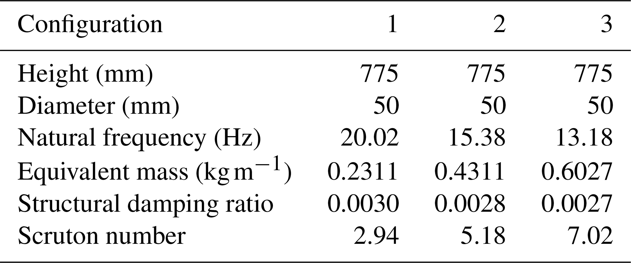
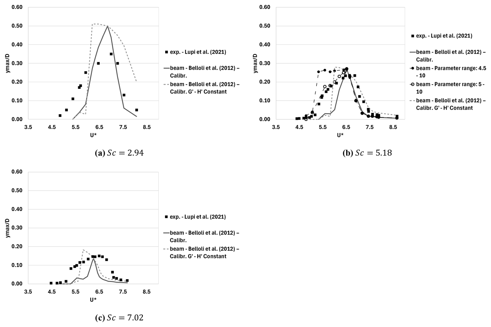
Figure 9 Maximum oscillation amplitudes normalized with respect to the reference diameter vs. U^∗ for the cantilever tower. Experimental results of Lupi et al. (2021) (solid squares) compared to predictions of the calibrated Hartlen–Currie model (continuous lines).

As shown in Figs. 9b, c and 10, the model accurately reproduces the maximum tip displacement for the two higher Sc values (Sc=5.18 and Sc=7.02). Comparing the Eurocode and the Blevins model highlights the Eurocode's behaviour in overpredicting the VIV response, whereas the opposite is observed with the Blevins model when they are used for a real-world cantilever structure. The calibrated Hartlen–Currie model as implemented in hGAST gives more accurate predictions albeit it is also conservative at the lowest Sc tested.

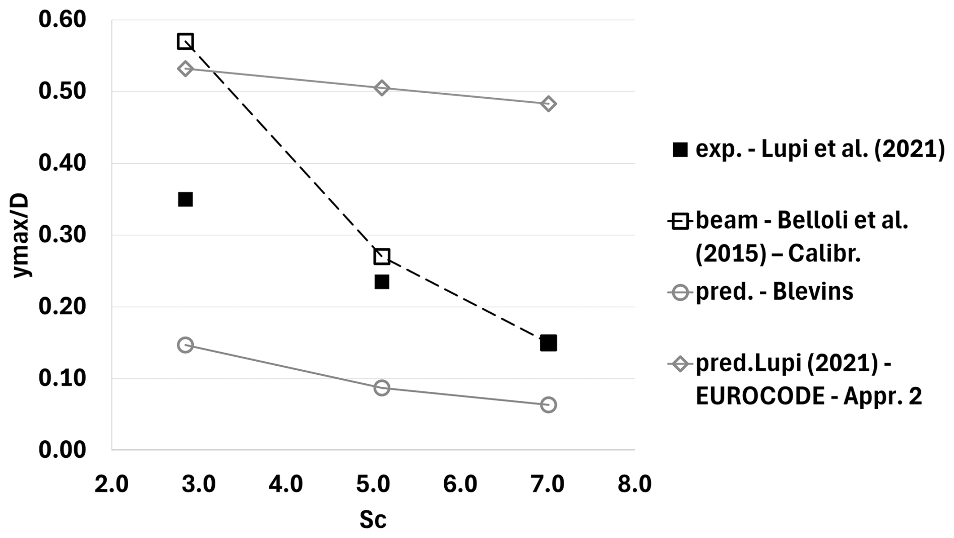
Figure 10 Maximum oscillation amplitudes normalized with respect to the reference diameter vs. Sc for the cantilever tower setup of Lupi et al. (2021) compared with the Hartlen–Currie-calibrated model, the Eurocode – Approach 2, and the predictions of the Blevins (1977) analytical formula.

More specifically, for Sc=2.94, it overpredicts the displacement by approximately 55%. The wind tunnel experimental results presented in Fig. 3 indicate that, for Sc≈ 3, the maximum vibration amplitude in the VIV response of a rigid elastically supported cylinder lies in the range of 0.4–0.5, which is significantly higher than the corresponding values reported in Lupi's experiment for the same Sc. This clearly demonstrates that the present results are governed by the experimental dataset used for model calibration. Furthermore, as indicated by the γ coefficient in Blevins' model (see Appendix B), which exceeds unity in the case of a cantilever beam, the maximum VIV tip amplitudes of a cantilever beam are expected to be higher than those of a rigid elastically supported cylinder. In addition, the predicted lock-in region is well captured for Sc=2.94, whereas it is considerably underpredicted for higher Sc values. This outcome also reflects the influence of the rigid-cylinder measurements used for calibration, which show a narrower lock-in region that decreases with increasing Sc. In contrast, for the cantilever case, increasing Sc primarily reduces the maximum displacement amplitude, while the lock-in range appears to remain essentially unchanged.

The underprediction of the lock-in region highlights a limitation: calibrations based solely on rigid-cylinder data are sufficient for estimating maximum amplitudes but inadequate for realistic cantilever elastic structures, such as wind turbine towers. The lock-in zone width depends on the rate at which the defining parameters vary towards zero from their calibrated value at $U_{max}^{\ast }$. To explore this sensitivity, two additional parameter ranges were tested. The baseline calculation used $U^{\ast }\in [\mathrm{5.5},\mathrm{9}]$ (in accordance with Belloli's wind tunnel tests), while two alternative ranges of $U^{\ast }\in [\mathrm{4.5},\mathrm{10}]$ and $U^{\ast }\in [\mathrm{5},\mathrm{10}]$ are also considered. Figure 9b compares the model response across the lock-in range for these different parameter zones. The model consistently links the predicted lock-in width to the span of the chosen parameter range. Specifically, a faster increase or decrease in the calibration constants shifts the predicted maximum VIV response to higher reduced velocities and produces a much steeper slope, failing to capture the gradual buildup of oscillations. In contrast, the decaying part of the oscillations (at higher U^∗ values) appears largely unaffected by the choice of parameter range.

4 Conclusions

The study presents the calibration and validation of a predictive engineering model for vortex-induced vibrations (VIV) in wind turbine towers, based on the Hartlen–Currie lift-oscillator formulation. The governing equations of the lift-oscillator model are expressed in a non-dimensional form to facilitate the calibration of the model's defining parameters. In this formulation, calibration is required only for specific sets of the problem's characteristic dimensionless parameters.

Model parameters are calibrated using experimental data obtained from rigid elastically mounted, untapered cylinders, enabling accurate prediction of vibration amplitudes and the wind speeds $U_{max}^{\ast }$ at which maximum VIV amplitudes occur, associated with lock-in phenomena. Integration of the calibrated model into a multibody aeroelastic solver demonstrates its capability to simulate VIV responses in elastic cantilevered cylinders, representing configurations relevant to real wind turbine towers. Comparisons with wind tunnel measurements show that the proposed model successfully predicts the maximum vibration amplitudes and the maximum response velocity of VIV. However, it tends to underestimate the width of the lock-in velocity range, particularly at higher Scruton numbers. This discrepancy does not indicate a shortcoming of the model itself, as it can be mitigated by refining parameter calibration using direct VIV wind tunnel measurements of the cantilever tower.

Furthermore, both the calibration and validation of the model rely on low-Reynolds-number wind tunnel data, significantly lower than those expected under full-scale wind turbine operating conditions, due to the lack of high-Reynolds-number experimental data. This does not constitute a limitation of the current work, as the model can be readily updated when such high-Reynolds-number data become available.

The present approach focuses on the first bending mode, while neglecting higher-order modes and the influence of ambient turbulence – factors identified as directions for future research. Overall, the calibrated Hartlen–Currie model provides a robust predictive tool that can be integrated into comprehensive aeroelastic design frameworks, enhancing the reliability and fatigue assessment of wind turbine towers subjected to vortex shedding excitation.

Appendix A: List of symbols

y	Crosswind tower elastic displacement
D	Tower diameter
l	Length of the cylinder
U	Inflow velocity
ρ	Air density
$\mathit{\eta }=y/D$	Non-dimensional crosswind tower elastic displacement
$\mathit{\tau }=tU/D$	Non-dimensional time parameter
m, c, k	Mass, damping, and stiffness of rigid elastically supported cylinder
$m_{\text{eq}}=m/l$	Equivalent cylinder mass
ζ	Damping ratio
ωs=2πfs	Vortex shedding frequency and angular frequency of the rigid cylinder
ωn=2πfn	Natural frequency and angular frequency of the elastic cylinder
G, H	Constants of the Hartlen–Currie model
$G^{\prime }=\frac{G}{{\mathit{\omega }}_{\mathrm{s}}}{H}^{\prime }=\frac{HD}{{\mathit{\omega }}_{\mathrm{s}}}$	Dimensionless constants of the Hartlen–Currie model
CL	Lift coefficient of the cylinder
CL0	Lift coefficient variation amplitude due to vortex shedding of the rigid cylinder case
$m^{\ast }=\frac{\mathrm{4}{m}_{\text{eq}}}{\mathit{\pi }\mathit{\rho }{D}^{\mathrm{2}}}$	Dimensionless mass ratio
$U^{\ast }=\frac{U}{f_{\mathrm{n}}D}$	Dimensionless flow velocity
$U_{max}^{\ast }$	Non-dimensional VIV maximum response flow velocity
$[U_{\text{low}}^{\ast }$, $U_{\text{high}}^{\ast }]$	Non-dimensional velocities lock-in range
$\mathit{Re}=UD/\mathit{\nu }$	Reynolds number
$\mathit{St}=\frac{f_{\mathrm{s}}D}{U}$	Strouhal number
$\mathit{Sc}=\frac{\mathrm{4}\mathit{\pi }{m}_{\text{eq}}\mathit{\zeta }}{\mathit{\rho }{D}^{\mathrm{2}}}$	Scruton number
Ucrit	Critical inflow velocity – corresponding to the shedding St number of the rigid cylinder

Appendix B: Blevins model

In the Blevins (1977) model, the peak amplitude during VIV is approximated by the following analytical expression, given as a function of the Sc and St numbers:

$$\begin{array}{}\text{(B1)}& y_{max}=\mathrm{0.07}D\mathit{\gamma }{\displaystyle \frac{\sqrt{\mathrm{0.3}+\frac{\mathrm{0.72}}{(\mathrm{1.9}+\mathit{Sc})\mathit{St}}}}{(\mathrm{1.9}+\mathit{Sc}){\mathit{St}}^{\mathrm{2}}}}.\end{array}$$

In the equation above, γ is a constant used to distinguish between different types of structures and supports. For a rigid cylinder, γ=1, whereas, for example, for the first mode of a cantilever beam, γ = 1.305.

Appendix C: Eurocode model – Approach 1

The Eurocode (European Committee for Standardization (CEN), 2005), approximates the maximum oscillation amplitude during VIV through the following analytical expression as a function of the Sc and St numbers:

$$\begin{array}{}\text{(C1)}& {\displaystyle \frac{y_{max}}{D}}={\displaystyle \frac{\mathrm{1}}{{\mathit{St}}^{\mathrm{2}}}}{\displaystyle \frac{\mathrm{1}}{\mathit{Sc}}}K{K}_{\mathrm{w}}{c}_{\text{lat}},\end{array}$$

where c_lat is the lateral force coefficient defined in the standard as a function of the Re, while K_w (the effective correlation length factor) and K (the effective mode shape factor) are given by

$$\begin{array}{}\text{(C2)}& \begin{array}{rl}& K_{\mathrm{w}}={\displaystyle \frac{{\sum }_{j=\mathrm{1}}^n{\int }_{L_{\text{cj}}}\left|{\mathit{\phi }}_{yi}\left(s\right)\right|\mathrm{d}s}{{\sum }_{j=\mathrm{1}}^m{\int }_{L_j}\left|{\mathit{\phi }}_{yi}\left(s\right)\right|\mathrm{d}s}},\\ & K={\displaystyle \frac{{\sum }_{j=\mathrm{1}}^m{\int }_{L_j}\left|{\mathit{\phi }}_{yi}\left(s\right)\right|\mathrm{d}s}{\mathrm{4}\mathit{\pi }{\sum }_{j=\mathrm{1}}^m{\int }_{L_j}{\mathit{\phi }}_{yi}^{\mathrm{2}}\left(s\right)\mathrm{d}s}},\end{array}\end{array}$$

and φ_yi is the ith bending mode shape in the cross flow direction that is excited by the vortex shedding, and L_j is the length of the structure between two nodes (see Fig. C1); for cantilevered structures, it is equal to the height of the structure, L_cj is the correlation length as defined in Fig. C1, n is the number of regions where vortex excitation occurs at the same time, and m is the number of antinodes of the vibrating structure in the considered ith mode shape φ_yi.

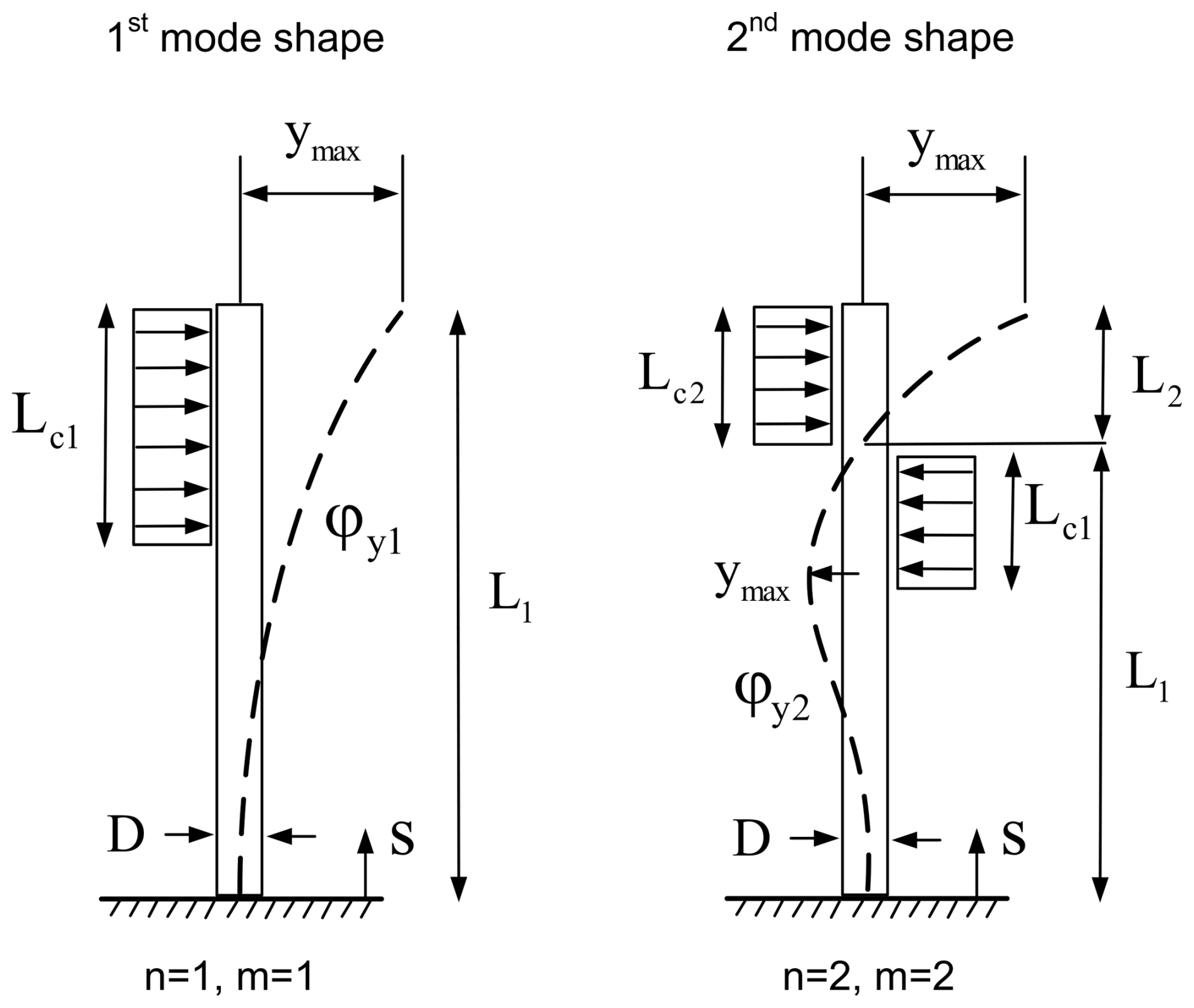
Figure C1 Definition of the correlation lengths in the case of the first and second modes of a cantilever beam.

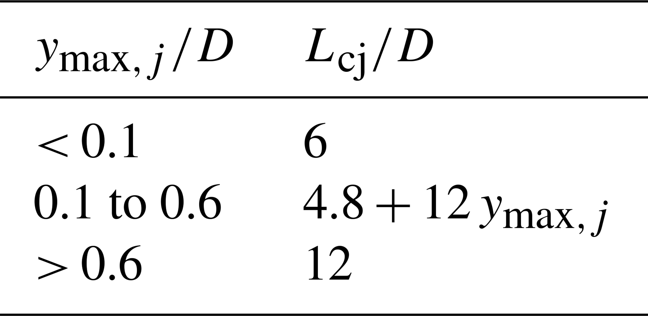
The effective correlation lengths L_cj are defined in Table C1.

Table C1 Definition of correlation length as a function of the maximum oscillation amplitude on either side of the antinode of the mode shape.

Appendix D: Eurocode model – Approach 2

In Approach 2 of the Eurocode (European Committee for Standardization (CEN), 2005), the maximum displacement is given by the expression

$$\begin{array}{}\text{(D1)}& y_{max}={\mathit{\sigma }}_{\mathrm{y}}{k}_{\mathrm{p}},\end{array}$$

where σ_y is the standard deviation of the displacement and k_p the peak factor. The standard deviation σ_y is given by

$$\begin{array}{}\text{(D2)}& {\displaystyle \frac{{\mathit{\sigma }}_{\mathrm{y}}}{D}}={\displaystyle \frac{\mathrm{1}}{{\mathit{St}}^{\mathrm{2}}}}{\displaystyle \frac{C_{\mathrm{c}}}{\sqrt{\frac{\mathit{Sc}}{\mathrm{4}\mathit{\pi }}-K_{\mathrm{a}}{\left(\mathrm{1}-\left(\frac{{\mathit{\sigma }}_{\mathrm{y}}}{b{a}_{\mathrm{L}}}\right)\right)}^{\mathrm{2}}}}}\sqrt{{\displaystyle \frac{\mathit{\rho }{b}^{\mathrm{2}}}{m_{\mathrm{e}}}}}\sqrt{{\displaystyle \frac{b}{h}}},\end{array}$$

where C_c is a constant dependent on the cross-sectional shape and for a circular cylinder also dependent on the Reynolds number, K_a is the aerodynamic damping parameter, a_L is the normalized limiting amplitude giving the deflection of structures with very low damping, Sc the Scruton number, St the Strouhal number, ρ the fluid density, m_e the mass per unit length, and h and b are the height and width of the structure. It should be noted that the aerodynamic damping parameter K_a is assumed to decrease with increasing turbulence intensity; therefore, for turbulence intensity % is taken equal to $K_{\mathrm{a},max}$.

The respective constants are given in Table E.6 of the Eurocode, which we include here for completeness.

Finally, k_p is given by

$$\begin{array}{}\text{(D3)}& k_{\mathrm{p}}=\sqrt{\mathrm{2}}\left\{\mathrm{1}+\mathrm{1.2}\arctan \left(\mathrm{0.75}{\left({\displaystyle \frac{\mathit{Sc}}{\mathrm{4}\mathit{\pi }{K}_{\mathrm{a}}}}\right)}^{\mathrm{4}}\right)\right\}.\end{array}$$

Table D1 Constants for the determination of the effects of vortex shedding (Table E.6 in Eurocode 1: Actions on Structures – Part 1-4: General actions – Wind actions).

Appendix E: Scanlan model

The one-equation model by Scanlan (1981) and Ehsan and Scanlan (1990) provides the maximum oscillation amplitude of a rigid elastically supported cylinder of Fig. 1 in the cross flow direction (single DOF of motion y) through the solution of the second-order dynamic equation:

$$\begin{array}{}\text{(E1)}& \begin{array}{rl}m\ddot{y}+c\dot{y}+ky& ={\displaystyle \frac{\mathit{\rho }}{\mathrm{2}}}{U}^{\mathrm{2}}Dl(H_{\mathrm{1}}\left(\mathrm{1}-\mathit{\epsilon }{\left({\displaystyle \frac{y}{D}}\right)}^{\mathrm{2}}\right){\displaystyle \frac{\dot{y}}{U}}\\ & +H_{\mathrm{2}}{\displaystyle \frac{y}{D}}+C_{\mathrm{L}\mathrm{0}}\sin \left({\mathit{\omega }}_{\mathrm{s}}t\right)).\end{array}\end{array}$$

The constants H₁ and H₂ and ε on the right-hand side of the equations are free parameters of the model that need to be specified by the user of the model. The additional stiffness term related to the constant H₂ can be neglected as it is small compared with the aerodynamic damping terms related to H₁. H₁ and ε, in turn, are determined from the experimental observation of two resonant response amplitudes $y_{max,\mathrm{1}}$ and $y_{max,\mathrm{2}}$ (or predictions of any analytical model), for two damping ratio values ζ₁ and ζ₂ and the corresponding Scruton numbers, Sc₁ and Sc₂. It can be readily shown that

$$\begin{array}{}\text{(E2)}& \begin{array}{rl}{H}_{\mathrm{1}}& ={\displaystyle \frac{\mathrm{8}\mathit{\pi }m\mathit{St}\left({\mathit{\zeta }}_{\mathrm{2}}{y}_{max,\mathrm{1}}^{\mathrm{2}}-{\mathit{\zeta }}_{\mathrm{1}}{y}_{max,\mathrm{2}}^{\mathrm{2}}\right)}{\mathit{\rho }{D}^{\mathrm{2}}\left(y_{max,\mathrm{1}}-y_{max,\mathrm{2}}\right)}}\mathit{\epsilon }\\ & ={\displaystyle \frac{\mathrm{4}({\mathit{\zeta }}_{\mathrm{2}}-{\mathit{\zeta }}_{\mathrm{1}})D^{\mathrm{2}}}{{\mathit{\zeta }}_{\mathrm{2}}{y}_{max,\mathrm{1}}^{\mathrm{2}}-{\mathit{\zeta }}_{\mathrm{1}}{y}_{max,\mathrm{2}}^{\mathrm{2}}}}.\end{array}\end{array}$$

Appendix F: Single Degree of Freedom Aerodynamic Damping Model

The Single Degree of Freedom Aerodynamic Damping Model (1DOF-ADM) (Lupi et al., 2018; Magnus et al., 2013) provides the maximum oscillation amplitude of a rigid elastically supported cylinder of Fig. 1 in the cross flow direction (single DOF of motion y) through the solution of the second-order dynamic equation:

$$\begin{array}{}\text{(F1)}& \begin{array}{rl}m\ddot{y}& +\mathrm{2}m{\mathit{\omega }}_{\mathrm{n}}\mathit{\rho }{D}^{\mathrm{2}}\left({\displaystyle \frac{\mathit{Sc}r}{\mathrm{4}\mathit{\pi }}}-K_{\mathrm{a}}\right)\dot{y}+ky\\ & ={\displaystyle \frac{\mathit{\rho }}{\mathrm{2}}}{U}^{\mathrm{2}}Dl{C}_{\mathrm{L}\mathrm{0}}\sin \left({\mathit{\omega }}_{\mathrm{s}}t\right).\end{array}\end{array}$$

The right-hand side term treats the aerodynamic lift as a harmonic excitation at the vortex shedding frequency – a justified simplification given the narrow-band nature of vortex shedding forces behind circular cylinders. The aerodynamic damping parameter K_a after Lupi et al. (2018) is expressed as an exponential function of the standard deviation of the oscillations σ_y in VIV:

$$K_{\mathrm{a}}=a{\displaystyle \frac{\exp \left(-b\frac{{\mathit{\sigma }}_{\mathrm{y}}}{D}\right)}{{\left(\frac{{\mathit{\sigma }}_{\mathrm{y}}}{D}\right)}^c}},$$

where the constants a, b, c are calibrated using experimental data and they are taken equal to

$$a=\mathrm{0.3475},b=\mathrm{5.808},c=\mathrm{0.3582}.$$