A numerical study of the influence of terrain on wakes, blockage, wind farm efficiency, and turbine efficiency

This study investigates the interplay of terrain, blockage, and wake effects using Reynolds-Averaged Navier–Stokes (RANS) simulations of 35 different combinations of terrain, wind farm layout, and atmospheric conditions. The terrain includes two idealized solitary ridgelines, an idealized valley, and flat ground. The wind farms comprise one or two rows of closely spaced turbines parallel to the terrain feature. We simulate these idealized wind farms in conventionally neutral boundary layers of different heights. The set of simulations also includes an existing onshore wind farm located along a ridgeline and run with stable and unstable surface conditions. The horizontal variation of the ground elevation (i.e., terrain) has a large influence on wake and blockage effects in this study. In addition, the predicted wind farm efficiency and turbine efficiency (power coefficient) vary significantly depending upon the terrain in the simulation and the position of the wind farm relative to the terrain. For single-row wind farms, the predicted effect of terrain on wind farm efficiency can exceed 4 % – for the simulated conditions. The separate but correlated effect of terrain on individual turbine efficiency is of a similar magnitude. Analysis of the results indicates that there are multiple physical drivers behind the efficiency trends, including streamwise pressure gradients and inviscid effects related to buoyancy. Energy prediction methods that do not account for these drivers have an elevated risk of producing large errors – at least at wind farms similar to those evaluated in the study.

1 Introduction

An energy yield analysis for a planned onshore wind farm requires two types of flow simulations: freestream and wind farm. Freestream simulations include terrain but not, by definition, wind turbines; wind farm simulations include turbines but usually not terrain. The objective of a freestream flow analysis is to translate processed wind measurements, typically taken at just a few on-site locations, to the expected freestream wind conditions at each one of the planned turbine locations. Together with a turbine power curve, these wind conditions are used to estimate the energy yield for each turbine were it to operate in isolation. The sum of the standalone turbine energy yields is called the gross energy of the wind farm. A wind farm flow analysis calculates how wakes and blockage modify the wind conditions experienced by the turbines. More to the point, it quantifies for each turbine how much the energy yield changes when the turbine is operating in the wind farm compared with isolated operation. This change is known as a turbine interaction loss, which is usually the largest loss contributing to the difference between the gross and net energy of a wind farm. While the effect of terrain on freestream (i.e., turbine-free) flow is a major consideration in energy yield assessments, the effect of terrain on wind farm flow – on wakes and on blockage – receives much less attention.

Several papers published over the last 15 years report results indicating that hills can substantially affect wind turbine wake recovery. These include studies based on Reynolds-Averaged Navier–Stokes (RANS) simulations (Politis et al., 2012), large-eddy simulations (LESs) (Shamsoddin and Porté-Agel, 2018a; Liu and Stevens, 2020; Patel et al., 2024), and wind tunnel measurements (Tian et al., 2013; Hyvärinen et al., 2018). The Shamsoddin and Porté-Agel (2018) paper also validated a pressure-gradient-sensitive reduced-order wake model against the hill LES results. Based on the validation and a follow-on sensitivity study, the authors concluded that hill-induced streamwise pressure gradients can have a strong influence on wake recovery – with favorable pressure gradients on the windward side of the hill promoting wake recovery and adverse pressure gradients on the leeward side slowing wake recovery. (A pressure gradient is favorable when pressure decreases in the direction of flow; it is adverse when pressure increases in the direction of flow.) Dar and Porté-Agel (2022a) further developed the reduced-order model and validated it against wind tunnel measurements of escarpment-affected wake flow. The results also pointed to the significant influence of terrain-induced pressure gradients on wake recovery.

Additional studies provide more direct evidence of streamwise pressure gradients influencing turbine wakes. Cai et al. (2021) varied the inclination of the floor of a wind tunnel to induce streamwise pressure gradients just downstream of a model wind turbine. Measured streamwise pressure variation was strongly correlated with and likely the cause of substantial differences in wake recovery. Favorable pressure gradients (FPGs) promoted wake recovery, and adverse pressure gradients (APGs) did the opposite. Bayron et al. (2023) induced streamwise pressure variation by adjusting the wind tunnel ceiling just downstream of the model turbine. The wake recovery was much slower in the APG wind tunnel configuration compared with the FPG configuration, with the zero pressure gradient (ZPG) wake recovery rate in between. In addition, the wake was vertically thicker and higher in the APG case compared with the ZPG case. The opposite trend was evident in the FPG case. Finally, Zhang et al. (2023) induced streamwise pressure gradients in LES by inclining the upper and lower walls to vary the cross-sectional areas of the domain along a row of four turbines aligned with the oncoming flow. They found that APGs made wakes deeper and wider, and FPGs did the opposite.

Beyond pressure, terrain can also affect turbulence, which influences wake recovery. Multiple papers have connected complex terrain with increased turbulence and, in turn, faster wake recovery (Politis et al., 2012; Dar and Porté-Agel, 2022b; Yang et al., 2015; Zhang et al., 2024).

Collectively, these studies show that terrain can substantially influence wake recovery. By implication, terrain can influence how much a turbine wake affects the wind speeds experienced by turbines located downstream, which affects wind farm efficiency. Other research, discussed below, suggests that the influence of terrain on the wake from an individual turbine also affects the wind conditions at the turbine itself. In other words, terrain can change turbine induction and thereby turbine power coefficient (i.e., individual turbine efficiency).

Before proceeding, we offer a brief aside to define the blockage-related terms used in this paper. Blockage is an obstruction to the otherwise free flow of air. In this paper, the obstruction relates to either a single turbine or a group of turbines. Blockage effects refer to the inviscid response of the flow to the obstruction. Perhaps the most salient blockage effect is the partial diversion of the flow around the turbine or turbines. The divergence of the streamlines starts upstream of the obstruction and directly connects with an upstream wind speed reduction via continuity. Further, the vertical deflection of the flow can perturb the stably stratified atmosphere in such a way as to significantly modify the blockage-related slowdown upstream of a wind farm (Lanzilao and Meyers, 2024). The terms “blockage” and “blockage effects” are often used interchangeably in the literature, and we will do the same here. Wind farm blockage refers to blockage from an array of wind turbines, and turbine blockage refers to blockage from an individual turbine. Induction is the turbine-blockage-related wind speed reduction upstream of the turbine; alternatively stated, it is the upstream wind speed reduction induced by the thrust force from an individual turbine. Induction factor is the fractional amount by which the wind speed at the rotor face of an isolated turbine is lower than the freestream wind speed. The definitions above reflect how the terms are used in this paper and are not intended to imply a universally accepted standard for blockage-related terminology. In the broader literature, the term “induction”, to take one example, is sometimes used to refer to a wind-farm-scale effect (e.g., Nishino and Dunstan, 2020); here, however, it refers exclusively to the effect of an individual turbine on wind speed upstream.

In LES results reported in Troldborg et al. (2022), the power coefficient of a standalone turbine was found to be sensitive to terrain-induced streamwise gradients. The turbine in this study was at the top of a ridgeline, and different streamwise gradients were achieved by varying surface roughness, which affected the separation downstream of the ridge. In simulations where the hub-height freestream wind speed downstream of the turbine location increased with distance from the turbine, the efficiency of the turbine was higher. When the simulated freestream wind speed decreased with distance downstream of the turbine, the efficiency was lower. The findings were similar in Zengler et al. (2024), a sensitivity study run with a RANS model, where a single turbine was simulated atop various idealized hill geometries with different surface roughnesses. In both of these studies, streamwise variation in the freestream wind speed downstream of the turbine was found to correlate with changes in induction factor and in turn power coefficient. Dar et al. (2023) used wind tunnel experiments to investigate the effect of streamwise pressure gradients on wakes and power performance. Fifteen different tunnel floor configurations were tested. These configurations induced streamwise pressure gradients, progressing from a strong APG case to a ZPG case and through to a strong FPG case. Pressure was not directly measured in the experiments; rather, it was inferred from the measured freestream wind speeds. In each configuration, the inferred freestream pressure gradient was nearly constant over a distance covering the induction zone of the model turbine through to the far wake. As the freestream streamwise pressure gradient increased, from the strong FPG case through the ZPG case and on to the strong APG case, the wake deficits generally also increased, while power coefficient generally decreased. For a given pressure gradient magnitude, an APG generally reduced turbine performance more than an FPG increased it. In an LES-based sensitivity study, Revaz and Porté-Agel (2024) simulated a standalone turbine atop various idealized hills. APGs downstream of the turbine increased wake deficits, which in turn increased turbine induction factor, decreasing power coefficient.

The impact of terrain on wind farm and turbine efficiency is still a relatively new field of study, with many opportunities to broaden the scope of the literature. Most of the research to date concerns wakes from a single turbine or a few aligned turbines. The results imply an effect of terrain on turbine interaction loss, but there is little in the literature directly making this connection through the analysis of full wind farms. In addition, the studies do not include the effect of buoyancy; the simulated and/or measured flow is always neutrally stratified. Yet wind farms are subjected to stably stratified flow all the time – if not within the boundary layer, then above it. This is significant because buoyancy effects profoundly modify the response of flow to terrain (Baines, 2022; Vosper, 2004; Bleeg et al., 2015b; Radünz et al., 2025) and to wind farms (Lanzilao and Meyers, 2024). Finally, the peer-reviewed literature does not address the potential impact of terrain on wind farm blockage, which can have a material impact on the wind speeds experienced by turbines in an array (Bleeg et al., 2018).

This contribution takes aim at these gaps. Using a RANS solver, we simulate full wind farms in different types of idealized terrain. The simulated boundary layers are neutral but with overlying stratification. From these simulations, we assess the influence of terrain on both wake and blockage effects. In turn, we evaluate the impact of terrain on turbine interaction loss across the wind farm. We also assess the impact of terrain on individual turbine efficiency. Finally, to better understand how the findings from these idealized simulations might translate to the field, we run additional simulations of a currently operating wind farm with inflow conditions derived from a numerical weather prediction model.

The next section of this paper, Sect. 2, explains the numerical approach used in this study. Section 3 presents the results, highlighting the effect of terrain on wakes, blockage, and energy conversion efficiency. The section also explores the main physical drivers behind the trends with terrain. Section 4 discusses the practical implications of the results and the limitations of the study. And, lastly, Sect. 5 summarizes the main findings.

2 Numerical approach

This section describes the flow modeling used in the investigation. It describes the flow equations, boundary conditions, and domain, as well as how wind turbines are represented in the simulations. It also includes information about the simulated wind farms, atmospheric conditions, and terrain – and a description of the mesh used to resolve these features. Lastly, the section explains the types of simulations run and how they are post-processed to assess whether and to what degree turbine and wind farm performance are influenced by terrain.

There are two types of wind farms in this study: idealized and real. The numerical analysis of idealized wind farms – comprising 31 different combinations of turbine layout, terrain, and inflow conditions – represents the heart of the study. The one real wind farm in the investigation involves far fewer simulations, the results of which are included here as a check on the representativeness and real-world applicability of the idealized wind farms results. This section applies to both types of wind farms; however, the subsections covering terrain (Sect. 2.2), wind farm layouts (Sect. 2.3), and atmospheric conditions (Sect. 2.4) apply primarily to the idealized wind farms. We address these three topics for the real wind farm in results Sect. 3.4.

2.1 RANS model

We constructed and customized the numerical model in STAR-CCM+, a general-purpose computational fluid dynamics code (Siemens PLM, 2022). The mass and momentum equations are steady-state incompressible RANS equations. The energy equation is a transport equation for potential temperature, and the turbulence equations are standard k-ε with modified coefficients. Buoyancy is included in the vertical momentum equation via a shallow Boussinesq formulation; the effect of buoyancy on turbulence is modeled with production terms in the turbulence equations. The horizontal momentum equations include the Coriolis force, and the vertical momentum equation has a source term designed to damp gravity waves near the lateral and top boundaries. More details about the flow model may be found in Bleeg et al. (2015a, b).

We represent the wind turbines with simple actuator disks. The thrust and torque, applied as body forces at each disk, are functions of the average axial velocity across the disk (U_disk). The derivation of these functions is discussed further in Sect. 2.3.

This model for wind farm flows has been validated against field observations related to wake and/or blockage effects at 17 wind farms, including those publicly reported in Bleeg et al. (2018, 2024) and Montavon et al. (2021, 2023, 2024).

Figure 1 Simulation domain with the ground surface colored by elevation (m).

2.2 Terrain definition and domain

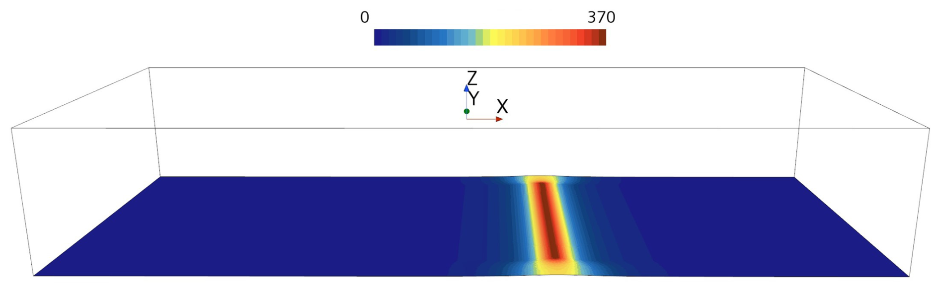
There are two primary terrain types in this study: flat and hill. In flat simulations, the ground elevation is uniformly equal to 0 m. In hill simulations, the ground elevation is a stretched Witch of Agnesi function (Eq. 1) extruded north and south to create a quasi-2D hill in the 3D RANS simulation. The height of the hill, h_c, is 370 m, and the base of the hill is at z = 0 m. The half-height, half-width of the hill, a, is 2100 m in all hill cases but one, where a is set to 1050 m. The maximum slopes of these two hills are 6.5 and 12.9°, respectively. The flow does not separate from the ground surface in any of the simulations run with these hills. The study also includes a valley terrain type, with the valley being a mirror image of the quasi-2D hill (h_c = −370 m).

$$\begin{array}{}\text{(1)}& z_{\text{ground}}={\displaystyle \frac{h_{\mathrm{c}}{a}^{\mathrm{2}}}{a^{\mathrm{2}}+x^{\mathrm{2}}}}\end{array}$$

The computational domain, depicted in Fig. 1, is large compared to the scales of the wind farm and hill profile. The length of the domain is 100 km, with the western boundary at x = −60 km and the eastern boundary at x = 40 km; the center of the quasi-2D terrain feature is at x = 0 km. The width of the domain is 40 km with the northern boundary at y = 20 km and the southern boundary at y = −20 km. The top boundary is at z = 17 km. The wind direction at hub height is approximately 270°, and the geostrophic wind is from the northwest. Thus, the western and northern boundaries are inflow boundaries, where we specify velocity, turbulence quantities, and potential temperature. The southern and eastern boundaries are outflow boundaries, where we specify static pressure. The top boundary is a slip wall set to a constant potential temperature. The bottom, ground boundary is a no-slip wall with a uniform aerodynamic roughness length of 0.028 m and a constant potential temperature of 283 K. The ground elevation is smoothed near the north and south boundaries, consistent with the standard practice for simulating flow over terrain with this RANS model.

2.3 Wind farm and turbine definitions

The idealized wind farms are organized in rows. Each row has 34 turbines, and the hub-to-hub spacing between neighboring turbines is two rotor diameters (2 D). The rows are north to south, perpendicular to the flow, and located either atop the hill crest, 15 D downstream of the crest, or 15 D upstream of the crest. The inter- and intra-row spacing is intended to be representative of wind farms in places with one dominant wind direction sector or two opposing dominant sectors. At these wind farms, the spacing between turbines in a row is typically 1.5 to 3.0 D; the distance between rows is typically 10 to 20 D. Such wind farms are common in Brazil, Chile, the US Southern Plains, the western US, and the Taiwan Strait. Tight spacing between turbines is also common when a wind farm is located along a ridgeline.

The turbine model has a hub height of 115 m, a rotor diameter of 160 m, and a rated power of 5.1 MW. The C_T and C_P curves, depicted in Fig. 2, are from the IEA-3.4-130 onshore reference turbine (Bortolotti et al., 2019).

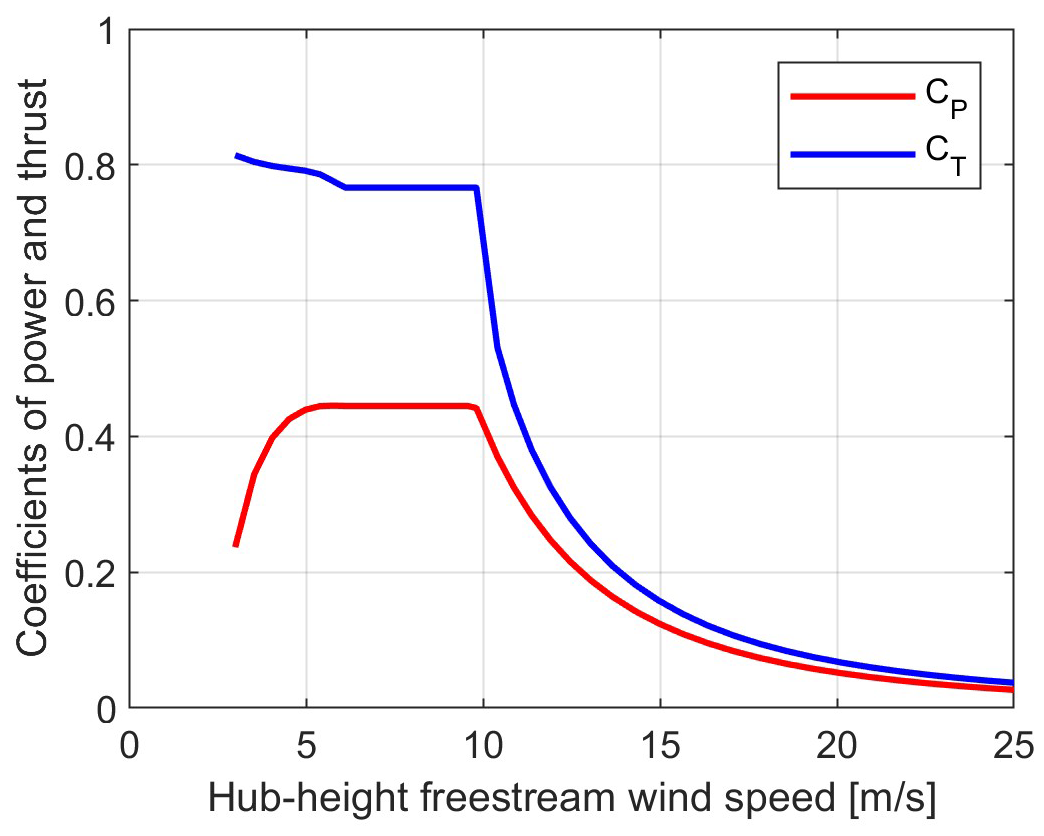
Figure 2 Nominal power and thrust coefficient curves for the wind turbine model simulated in the idealized wind farms.

These curves, which are functions of hub-height freestream wind speed, must be converted to functions of U_disk to be used in the wind farm simulations. We make the conversion using a procedure similar to that described in van der Laan et al. (2014). It involves running single-turbine simulations in flat terrain over a set of wind speeds spanning the operating range of the wind turbine. In these simulations, where hub-height freestream wind speed is known, the actuator disk forces are set according to the original performance curves (Fig. 2). At the end of each simulation, we record U_disk. The outcome of this procedure is a set of curves for power, thrust, and rotor speed specified as functions of U_disk. These curves form a look-up table used to control the actuator disks during wind farm simulations and to support the post-processing of the results. We refer to this table as the turbine performance look-up table. This procedure is used to generate the turbine performance look-up tables for both the idealized and the real wind farm simulations.

The table includes an additional column: effective wind speed, U_e. For a given value of U_disk and corresponding values of thrust and power, U_e is the wind speed that yields the same power and thrust when using the original C_T and C_P curves. We use this quantity to help analyze the RANS results in Sect. 3.1.

2.4 Atmospheric conditions

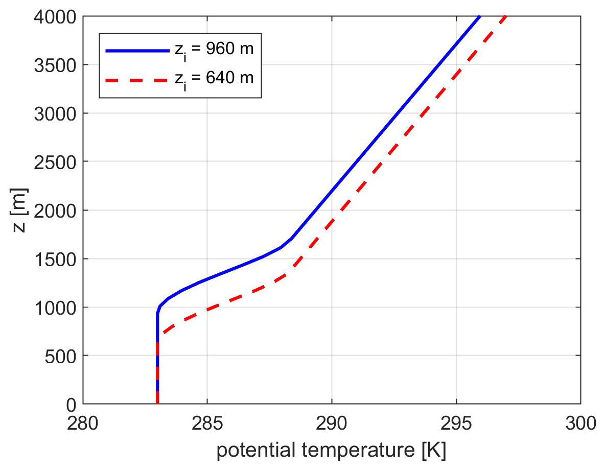
The atmospheric conditions in the idealized wind farm simulations feature stable stratification overlying a neutral boundary layer. The stratification starts with a capping inversion approximately 600 m thick with a maximum potential temperature lapse rate of 10 K km⁻¹. The free atmosphere above has a potential temperature lapse rate of 3.3 K km⁻¹. Nearly all the conventionally neutral boundary layers simulated in this study use one of the two inflow potential temperature profiles depicted in Fig. 3. The primary difference between the profiles is z_i, the altitude at which the inversion starts. In one profile, z_i is 640 m; in the other, z_i is 960 m. We use a single-column (one-dimensional) RANS model to generate velocity and turbulence profiles that are in quasi-equilibrium with the prescribed potential temperature profile, given inputs such as latitude (= 43°), aerodynamic roughness length (= 0.028 m), and geostrophic wind speed. In each case, the geostrophic wind speed is set such that all the turbines in the simulated wind farm operate on the flat part of the C_T curve. The inflow profiles of velocity and turbulence are uniform above the inversion.

Figure 3 Inflow vertical profiles of potential temperature.

2.5 Mesh

The vertical spacing of the prismatic cells used to resolve the boundary and inversion layers relaxes from a cell height of 2 m at the ground to a cell height of 92 m or less at the top of the inversion layer. Above the inversion, the mesh further relaxes to isotropic cells with centroid spacings of approximately 200 m.

The horizontal mesh resolution is highest near the wind farm. The cell spacing is no more than 0.1 D within 12 rotor diameters of any turbine up to a height of 335 m. The cell spacing in close proximity to the actuator disks is 0.05 D.

2.6 Wind farm and turbine performance metrics

The ultimate aim of this study is to better understand whether and to what degree terrain influences wind farm and turbine performance. The primary performance metric for the wind farm is array efficiency, which is defined as follows:

$$\begin{array}{}\text{(2)}& \mathit{\eta }={\displaystyle \frac{{\sum }_{k=\mathrm{1}}^N{P}_{\text{WF},k}}{{\sum }_{k=\mathrm{1}}^N{P}_{\mathrm{I},k}}}.\end{array}$$

Here, P_WF,k is the power from turbine k when simulated in the wind farm, and P_I,k is the power from turbine k when simulated in isolation. The terms array efficiency and wind farm efficiency are used interchangeably in this paper. We also refer to η as a turbine interaction loss factor. The percent turbine interaction loss, L, is simply 100 % × (1−η).

Reliably calculating the values in Eq. (2) requires results from three types of simulations: wind farm (all actuator disks on), freestream (all actuator disks off), and isolated turbine (one actuator disk on). All three types are run for each combination of simulated terrain, atmosphere, and turbine layout – using the same domain, mesh, and boundary conditions. The wind farm simulation yields the P_WF,k values. To get the P_I,k values, we could run an isolated turbine simulation at each turbine location in the wind farm layout, but this is not necessary. Instead, we run a subset of the turbines in isolation, typically four turbines – one simulation per turbine. Using results from the freestream simulation together with the isolated turbine results, we can determine the relationship between the freestream conditions and U_disk for the isolated turbines. This enables reliable estimation of ${U_{\text{disk}}}_{\mathrm{I},k}$ and, in turn, P_I,k for every turbine. As will be discussed in Sect. 3.3, the relationship between freestream conditions and ${U_{\text{disk}}}_{\mathrm{I},k}$ can be sensitive to the position of the turbine relative to the hill profile, so when simulating two rows on a hill, two sets of isolated turbine simulations are needed – one for each row.

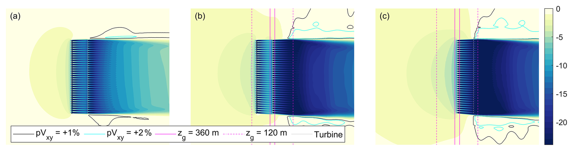
Figure 4 Top view of the percent change in wind speed relative to freestream at hub height for the flat (a), hill windward (b), and hill leeward case (c). Magenta lines are ground elevation contours; the hill crest is located between the two solid magenta lines.

The primary turbine performance metric is power coefficient:

$$\begin{array}{}\text{(3)}& C_P={\displaystyle \frac{P_{\mathrm{I}}}{\frac{\mathrm{1}}{\mathrm{2}}\mathit{\rho }A{U}_{\mathrm{\infty },\text{disk}}^{\mathrm{3}}}}.\end{array}$$

Here, P_I is the power from a turbine simulated in isolation, ρ is the density, and A is the swept area of the rotor. U_∞,disk is the axial component of velocity averaged over the disk in the freestream simulation. C_P values reported herein correspond to an average of the isolated turbine simulations run for any given terrain–atmosphere–turbine-row combination. Note that there are two types of power coefficient discussed in this paper: calculated and nominal. When referring to calculated power coefficient values (i.e., those from Eq. 3), C_P is italicized. When referring to a nominal power coefficient curve or a value from that curve, C_P is not italicized.

The power values used in Eqs. (2) and (3) are not the dot product of thrust and velocity at the actuator disk; the power instead derives from U_disk and the turbine performance look-up table.

3 Results

Here we present the simulation results, dividing them into four sections. Results from the idealized two-row wind farms and idealized single-row wind farms are in Sect. 3.1 and 3.2, respectively. These sections focus on the impact of terrain on wakes, wind farm blockage, and turbine interaction loss. The third section, Sect. 3.3, presents results from turbines simulated in isolation and focuses on the impact of terrain on the near wake, turbine blockage, and turbine efficiency (C_P). Results from simulations of a real wind farm are in Sect. 3.4.

This Results section includes many plots of and references to “wind speed” and “pressure”. Here, wind speed is the horizontal component of velocity. Pressure is relative pressure. This relative pressure is equal to the absolute pressure minus the pressure field in balance with both the geostrophic Coriolis force and the inflow potential temperature profile. This section also includes many references to height, which here means the vertical distance above the local ground level. For example, a hub-height surface is one where all points on the surface are 115 m directly above the local terrain.

3.1 Two-row wind farms

We simulate three different two-row wind farms: flat, hill windward, and hill leeward. The turbines in each row are arranged south to north, with the second row directly to the east of the first row. The x component of the distance between the rows is 15 D. In the flat case, the wind farm operates in flat terrain. In the hill windward case, the first row is on the windward side of the hill and the second row is on the crest. In the hill leeward case, the first row is on the crest and the second row is on the leeward side of the hill. The hill windward and hill leeward cases are run with the same inflow conditions. In the freestream simulations, the hub-height wind speed is 9 m s⁻¹ at the crest, 6.2 m s⁻¹ 15 D upstream of the crest, and 6.8 m s⁻¹ 15 D downstream of the crest. In the flat case, the freestream hub-height wind speed is 9 m s⁻¹ across all turbine locations. In all three cases, z_i = 960 m.

Figure 5 Percent change in wind speed relative to freestream on a vertical plane located 2.5 D upstream of the second row in the flat (a), hill windward (b), and hill leeward cases (c). Dashed lines demark the rotor layer (heights of 35 and 195 m). The thin white lines indicate the height of the maximum wind speed deficit for each constant-y gridline in the discretized solution.

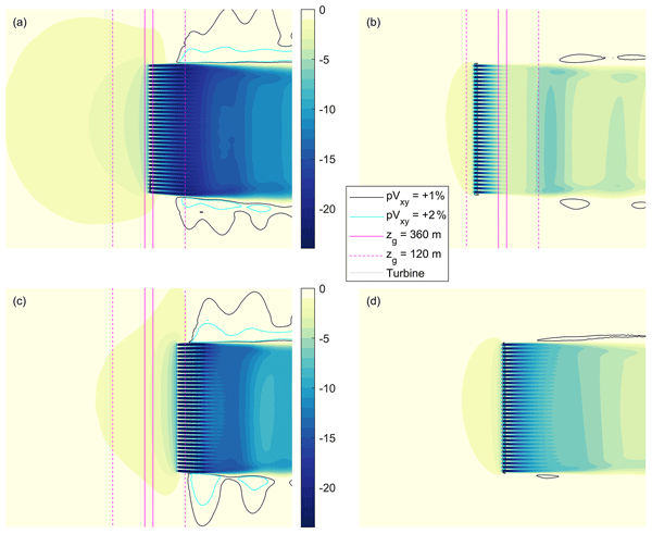
Terrain has a significant impact on wake recovery and upstream blockage effects in these simulations. This can be seen in Fig. 4, which shows on hub-height surfaces the percent change in wind speed due to the presence of the wind farm (flow is from left to right, as is the case in all top-view plots in this paper). The wakes downstream of the hill windward and hill leeward wind farms are clearly deeper than in the flat case. In addition, the upstream slowdowns are more pronounced and far-reaching in the hill cases, especially the hill leeward case. Finally, a close look at Fig. 4 reveals that the wakes in between the two rows are deeper in the hill leeward case than in the hill windward case – with the flat case in between. The case-to-case differences in the wakes from the first row can be seen more clearly in Fig. 5, which shows the percent change in wind speed relative to freestream on a vertical plane 2.5 D upstream of the second row.

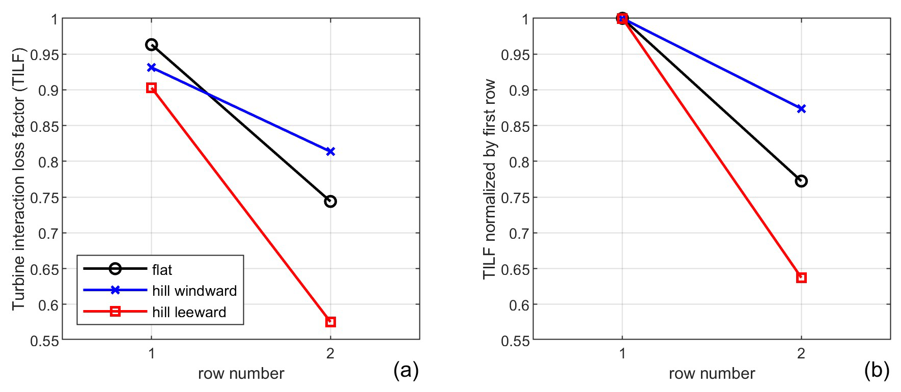
Figure 6 Turbine interaction loss factor, η, by row (a); turbine interaction loss factor normalized by the turbine interaction loss factor for the first row (b).

The wake and blockage trends in Fig. 4 are reflected in the row-by-row performance. This can be seen in Fig. 6. The first row in the hill leeward case is less efficient than the first row in the hill windward case, which is less efficient than that first row in the flat case. This order is consistent with the apparent strength of the upstream blockage effects in Fig. 4. The hill leeward case also has the least efficient second row; the hill windward case has the most efficient second row. The efficiency of the second row relative to the first row is clearly very sensitive to terrain, as highlighted in Fig. 6b. A significant contributor to this efficiency trend is differences in streamwise pressure variation.

The hill induces substantial streamwise pressure gradients in the vicinity of the wind farm. Figure 7 shows how the freestream pressure varies along the hill profile (flow is from left to right, as is the case in all similar plots in this paper). The pressure gradient is favorable on the windward side of the hill and generally unfavorable (adverse) on the leeward side. As discussed in the Introduction, FPGs promote wake recovery; APGs do the opposite. The wakes from the first row in the hill windward case travel through a favorable pressure gradient before reaching the second row. The pressure drop between these rows accelerates wake recovery, and as a result, the second row experiences less turbine interaction loss. The wakes from the first row in the hill leeward case travel primarily through an APG, deepening the wakes and increasing the turbine interaction loss in the second row. The freestream streamwise pressure gradient in the flat case is negligible, and the turbine interaction loss in the second row relative to the first naturally falls between the two other cases (Fig. 6b).

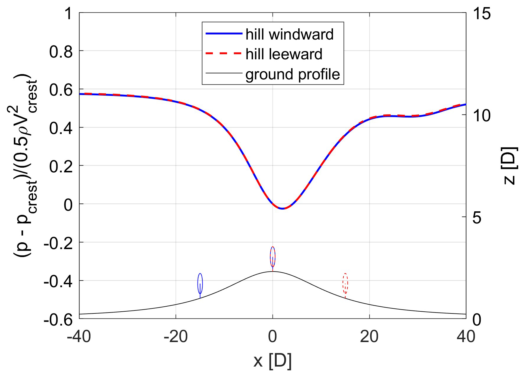
Figure 7 Freestream pressure coefficient along the hill profile at hub height in the middle of the domain (y = 0 m) for the hill windward (blue) and hill leeward (red) cases. The pressure coefficient is relative to conditions at the hill crest. The thin black line is the hill profile. Turbine icons matching the legend colors represent the locations of the turbine rows for each case.

Terrain can also affect the trajectory of a wake. In the hill leeward case, the wakes from the first row are clearly higher than in the other two cases (see Fig. 5). The wakes from the first row in the hill windward case are slightly lower than those in the flat case. These differences must have some effect on the turbine interaction loss trends in Fig. 6, but the effect is probably small compared with the effect of the wake deficit differences evident in Fig. 5. The average deficit along the maximum-deficit white lines in Fig. 5 is 12 % for the flat case, 9.6 % for the hill windward case, and 19.5 % for the hill leeward case. When these deficits are run through the turbine power curve, they translate to power loss factors of 0.68, 0.74, and 0.52, respectively. These trends strongly resemble the case-to-case variation in turbine interaction loss factor for the second row, seen in Fig. 6a (0.74, 0.81, and 0.57, respectively), suggesting that despite some differences in the vertical positions of the wakes between the cases, differences in the magnitudes of the wake deficits still appear to be the main driver behind the power loss trends across these simulations. The effect of terrain on wake trajectory may be more important at wind farms located in more complex terrain.

Terrain can also affect turbulence, which influences wake recovery. The mean freestream turbulence intensity (TI) across the disk areas in the flat case is 8.6 %. For the hill windward case, the freestream TI is 7.5 % at the first row and 4.9 % at the second row. For the hill leeward case, the freestream TI is 4.9 % at the first row and 8.6 % at the second row. In an effort to better understand the relative contributions of turbulence and pressure to the recovery of the wake between first and second row of turbines in these three cases, we conducted a control volume analysis (CVA) of the RANS solutions. The following is a brief summary of the analysis; a more complete description is in the Appendix.

The control volume corresponds to the rotor layer with the western surface 2.5 D downstream of the first row and the eastern surface 2.5 D upstream of the second row. The turbulent transport of momentum is the primary contributor to wake recovery in the flat case (Fig. A2a). The wind-farm-induced pressure field, in contrast, materially works against wake recovery between the first and second row, consistent with findings reported in Bastankhah et al. (2024). In the hill windward case, the turbulent transport of momentum makes a smaller contribution to wake recovery compared with the flat case, yet there is more wake recovery in the hill windward case (Fig. A2b). The stronger wake recovery in this case is primarily due to the significant pressure drop between the west and east surfaces. In the hill leeward case, the turbulent transport of momentum makes a smaller contribution to wake recovery than in the flat case, consistent with the larger wake deficits evident in the hill leeward case (Fig. A2c). However, the trend in turbulent diffusion is not sufficient to explain the fact that the wakes are deeper just upstream of the second row than just downstream of the first. The significant pressure rise from the western surface to the eastern surface is the primary reason for this. Lastly, the large differences in wake recovery between the hill windward and hill leeward cases are not due to hill-induced turbulence, as the contributions of turbulence to wake recovery in these two cases are about the same; it is instead differences in the hill-induced pressure fields that explains the differences in wake recovery. (The results in Fig. A2 suggest that the vertical advection of momentum is also a substantial contributor to wake development in the rotor layers across the three cases; however, as explained in the Appendix, this contribution is linked with the contributions of pressure and the turbulent transport of momentum). Most of the commonly used engineering models for wind farm flow include consideration of TI, and, depending upon the quality and fullness of the site-specific ambient TI input data, these models may capture some of the impact of terrain-induced turbulence changes on wake recovery. However, none of the commonly used models account for terrain-induced pressure, which can have a large influence on turbine wakes.

We also calculate turbine interaction loss, 100 % × (1−η), for the full wind farm. The turbine interaction loss is 14.6 % in the flat case. It is 15.8 % in the hill windward case and 18.5 % in the hill leeward case. In a typical energy yield analysis, the turbine interaction loss for a wind farm in terrain would be estimated using an engineering model that does not directly include the effect of terrain on wakes and blockage. If we were to neglect the influence of ground elevation variation in this RANS-based analysis and use the flat case result (L = 14.6 %) to predict the losses for the two hill cases, the losses would be underestimated, especially for the hill leeward case. That said, in a typical energy yield analysis, the turbine interaction loss calculation would consider how the freestream wind speed varies over the terrain.

There does not appear to be a standard approach for incorporating terrain-induced spatial wind speed variations in a wind farm flow analysis run with a model that does not include terrain. Brogna et al. (2020) add wake deficits to the local background wind speed. Farrell et al. (2021) and Lanzilao and Meyers (2022) multiply the local background wind speed by wind speed loss factors. Here we explore both of these hybrid approaches using the freestream RANS solution for the quasi-2D hill in combination with the RANS solution for the two-row wind farm in flat terrain.

We start with the multiplicative approach used in Farrell et al. (2021) and Lanzilao and Meyers (2022). From the flat case analysis, we can determine the effective wind speed experienced by each turbine relative to the effective wind speed each turbine would experience operating in isolation $(U_{\mathrm{e}}/U_{\mathrm{e},\mathrm{I}}{)}_{\text{flat}}$. We determine ${U_{\mathrm{e},\mathrm{I}}}_{\text{hill}}$ for each turbine from the freestream and isolated turbine simulations run with the hill terrain, as described in Sect. 2.6. Multiplying the two sets of values yields ${U_{\mathrm{e}}}_{\text{hill\hspace{0.17em}\hspace{0.17em}estimate}}$ for each turbine. As explained in Sect. 2.3, the U_e values can be used to look up power. These power values yield hybrid hill-flat turbine interaction loss predictions of 20.3 % for the hill windward case and 9.6 % for the hill leeward case. These hybrid predictions are significantly different from the loss values derived from simulations of the wind farms with the terrain included. Not only are the errors large but the windward-to-leeward loss trend is also dramatically reversed. Lanzilao and Meyers (2022) cautioned that the multiplicative approach may not work well when there are large variations in the background velocity, which is the case here.

If we instead add the deficits to the local background wind speed (${U_{\mathrm{e}}}_{\text{hill\hspace{0.17em}\hspace{0.17em}estimate}}={U_{\mathrm{e},\mathrm{I}}}_{\text{hill}}+(U_{\mathrm{e}}-U_{\mathrm{e},\mathrm{I}}{)}_{\text{flat}}$), the results improve. This add-deficits hybrid approach predicts a 15.7 % loss for the hill windward case, nearly matching the result from the actual hill windward case. The add-deficits prediction for the hill leeward case, however, is still too low: 10.1 % vs. 18.5 % for the actual case.

These results indicate that there are pitfalls in simple hybrid approaches that can lead to large prediction errors; having said that, the above examples miss an important part of how the hybrid approach would likely work in practice. Most engineering models for wind farm flows take in local TI as an input, whereas in the above example, the RANS simulation providing the wind farm flow result is run with freestream TI that is higher than the freestream TI levels at the turbine locations in the hill windward and hill leeward cases. Accounting for the hill-induced spatial variation of TI would probably improve the hybrid results – though again, the benefit would likely be limited by the fact that hill-induced pressure gradients, which are unaccounted for in most engineering models, have a larger influence on the case-to-case wake trends.

3.2 Single-row wind farms

We ran 28 single-row RANS-based wind farm flow analyses, varying row location, terrain, and inflow conditions. Table 1 lists the high-level results for these cases. The turbine interaction loss, L, varies a great deal across these single-row wind farms, from −1.8 % to +15.6 %. The following pages and figures explore the RANS results in more detail in order to better understand this variation and how it relates to wakes, blockage, and terrain.

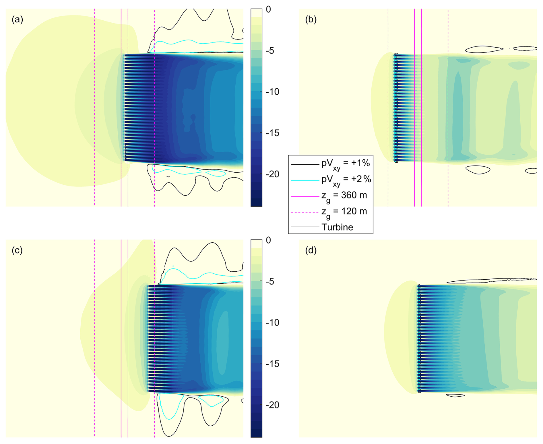
Figure 8 Top view of the percent change in wind speed relative to freestream at hub height for Case A (a), Case B (b), Case C (c), and Case D (d), as defined in Table 1. Magenta lines are ground elevation contours; the hill crest is located between the two solid magenta lines.

We first look at cases A–D, which are all simulated with a z_i of 960 m. Differences in wake and blockage effects across these cases can be seen in Fig. 8, which shows top views of the percent change in wind speed relative to freestream conditions at hub height (i.e., on hub-height surfaces). The wake recovery and upstream blockage effects are much different in the cases with the hill compared with the flat-terrain case. When the turbine row is on the crest or on the leeward side of the hill (Fig. 8a, c), the upstream blockage effects are much more pronounced than in the flat case (Fig. 8d), and the wind farm wake downstream is deeper. In contrast, when the turbine row is on the windward side of the hill (Fig. 8b), the wind farm wake deficit is smaller than in the flat case, and the upstream blockage effect is less pronounced.

The Case A results relative to Case D are consistent with the RANS results in the master's thesis of Kashyap (2022), which found that the upstream blockage effect of an infinitely long row of wind turbines can be stronger when the row is located along the crest of a quasi-2D hill as compared to when located in flat terrain.

Table 1 Case descriptions and performance values from the 28 single-row wind farm analyses. U_in is the hub-height wind speed at the inflow boundary; W_g is the geostrophic wind speed; and C_P,WF is the wind farm power coefficient.

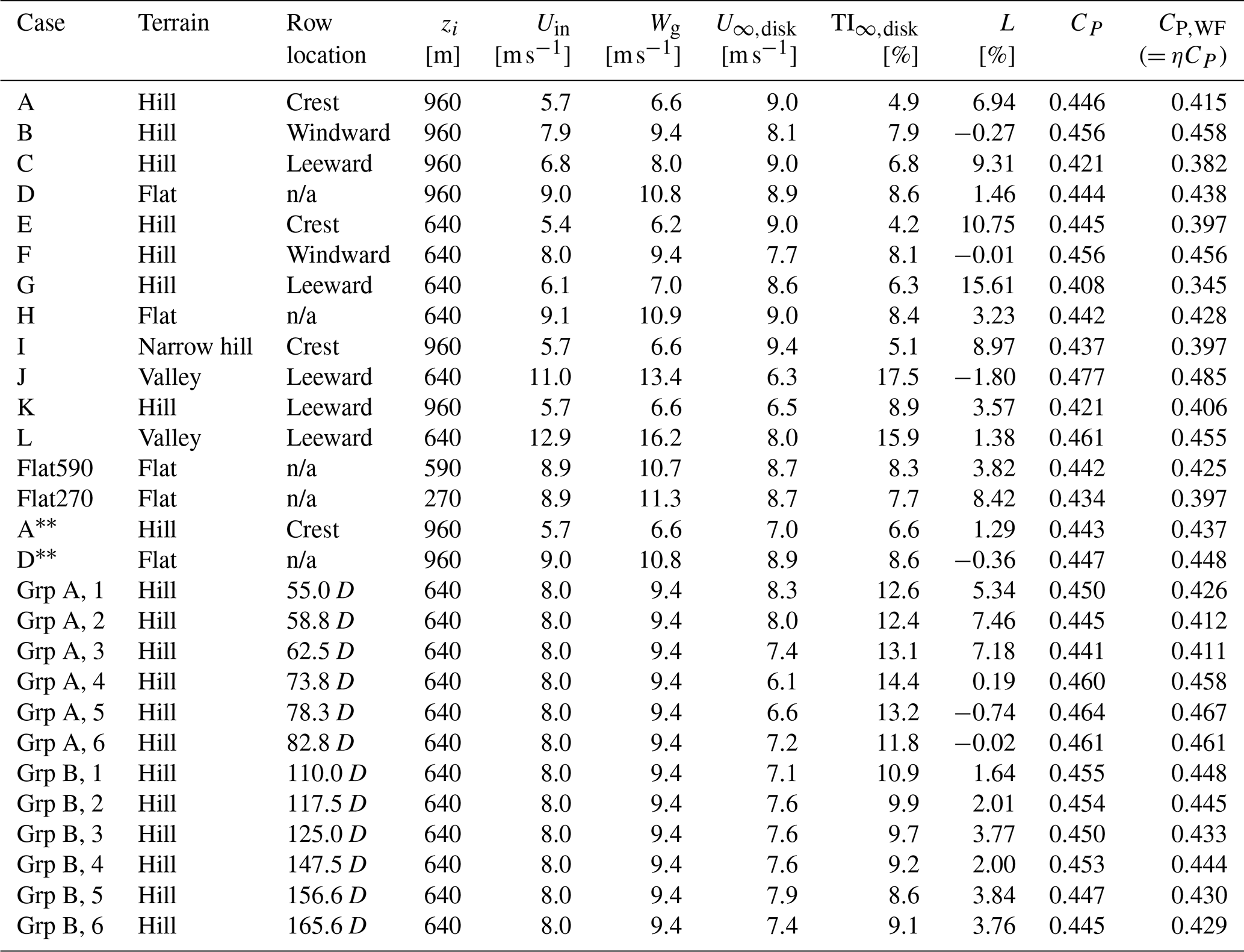
n/a: not applicable.

The hub-height plots in Fig. 8 are intended to show the effect of terrain on blockage and wakes. In this section, there are 11 of these top-view hub-height plots, which correspond to the first 11 cases in Table 1. To supplement these plots, and in consideration of the expected effect of terrain on wake trajectory, Fig. A3 (at the end of the Appendix), shows the wake deficits on constant-x vertical planes 8 D downstream of the turbine row for each of the 11 cases. These plots confirm that terrain affects the vertical trajectory of the turbine wakes, but they also indicate that the top-view hub-height plots in this section provide a reasonable representation of how the wake deficits vary from case to case through the rotor layer, at least close to the wind farm.

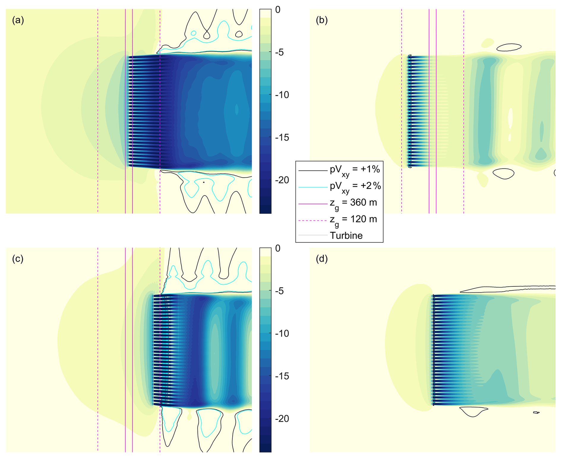
Figure 9 Top view of the percent change in wind speed relative to freestream at hub height for Case E (a), Case F (b), Case G (c), and Case H (d), as defined in Table 1. Magenta lines are ground elevation contours; the hill crest is located between the two solid magenta lines.

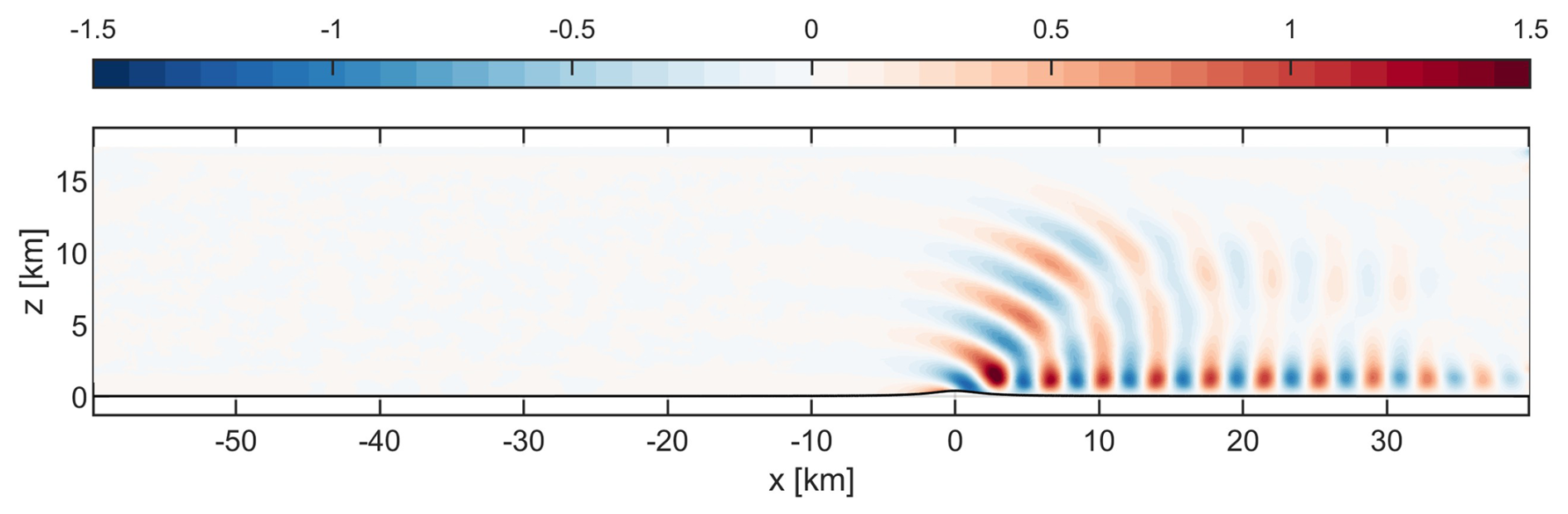
Figure 10 Case G, side view of the vertical component of freestream velocity [m s⁻¹] near the middle of the domain (y = 160 m).

Figure 9 shows the percent change in wind speed relative to freestream for cases E–H; these cases are similar to cases A–D but with z_i = 640 m. Compared with the z_i = 960 m results in Fig. 8, the case-to-case trends in wake and blockage effects in Fig. 9 are similar but more pronounced – as are the case-to-case loss trends (compare cases E–H with cases A–D in Table 1). The effect of gravity waves is also more clearly evident in Fig. 9, especially for the case with the row on the leeward side of the hill (Case G). Figure 10 shows the vertical component of velocity in a side view of the freestream solution for this case. Hill-induced gravity waves can be seen in the figure. Despite the large amplitude of these waves, there is no indication of gravity waves reflecting off a boundary and polluting the results in this case or in any of the other cases in this study.

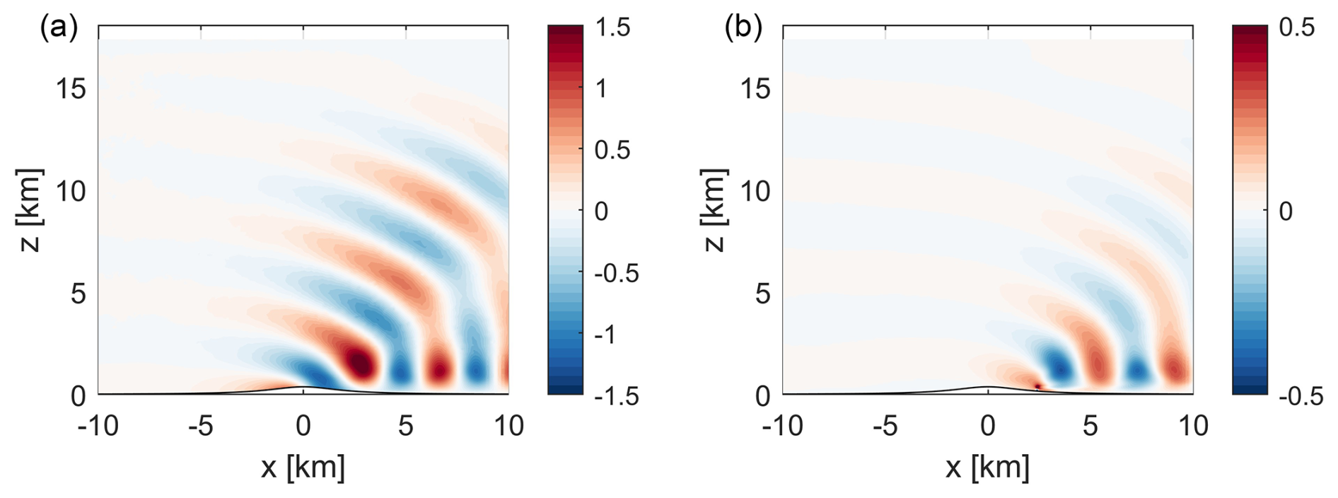
Figure 11 Case G, side view of the vertical component of velocity [m s⁻¹] near the middle of the domain (y = 160 m): freestream solution (a); wind farm solution minus freestream (b).

The wind farm also induces gravity waves, a finding consistent with Allaerts and Meyers (2019). Figure 11a is a reproduction of Fig. 10 but zoomed in; Fig. 11b is from the same case but shows the wind farm solution minus the freestream solution, revealing the effect of the wind farm on the vertical component of velocity. The gravity waves induced by the wind farm have similar characteristics to the gravity waves induced by the hill but with a lower amplitude and, because the wind farm is 15 D downstream of the crest, a different initiation point and phase.

Differences in the upstream blockage effects evident in Figs. 8 and 9 are consistent with the differences in turbine interaction loss across the same eight cases in Table 1. The upstream blockage effects are, of course, the cause of turbine interaction loss in single-row wind farms. The rest of this subsection focuses on how terrain modulates these upstream effects.

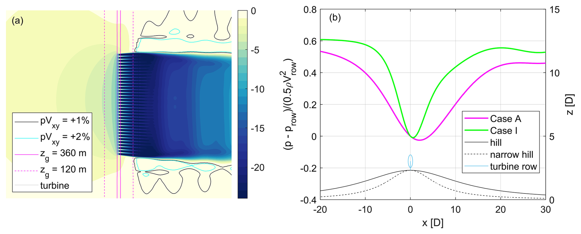
Figure 12 Top view of the percent change in wind speed relative to freestream at hub height for Case I (a) and freestream pressure coefficient along the hill profiles at hub height at y = 0 m (b). Case I (narrow hill) is in green. Case A (hill) is magenta. The pressure coefficient is relative to conditions at the hill crest, where the wind turbines in the corresponding wind farm simulations are located. The thin black lines depict the two hill profiles.

We begin this effort with an analysis featuring a hill that is narrower than the baseline hill. Case I is similar to Case A (z_i = 960 m with the turbines on the hill crest), but it has a hill profile that is half as wide. Figure 12a shows the percent change in wind speed relative to freestream for Case I, and Fig. 12b shows the streamwise freestream pressure variation for both the narrow hill case (Case I) and the similar baseline hill case (Case A). Compared with the baseline hill, there is a sharper pressure rise downstream of the crest of the narrow hill case. This deepens and expands the wake downstream, increasing the wake blockage, which appears to contribute to an increase in the upstream blockage effect and, in turn, a larger loss for the narrow hill case.

The concept of wake blockage is well known among those who conduct wind tunnel experiments, but it is seldom discussed in the wind energy community. Blockage is an obstruction causing oncoming flow to diverge from the path it would otherwise take. The obstruction need not be solid – a local region of relatively slow-moving flow can have a similar effect. In this discussion, the slow-moving flow feature is the wind farm wake. According to the continuity equation, the presence of the wind farm wake means that flow must diverge and slow upstream. Because hill-induced streamwise pressure gradients affect the wind speed in the wake and the size of the wake, it also affects how much oncoming flow is deflected relative to freestream conditions. This deflection cannot happen discontinuously. It happens over a distance, a distance that could include locations upstream of the wind farm. In other words, according to this theory, wake blockage, which can be modified by streamwise pressure gradients, influences the blockage-related slowdown upstream of the wind farm. These slowdowns in turn affect the wind speeds experienced by the turbines and the turbine interaction loss. A similar theory was put forward in Revaz and Porté-Agel (2024) to explain the effect of streamwise pressure gradients on the induction of an individual turbine; however, to our knowledge, the theory has not, until now, been applied to wind farm blockage in terrain. This theory is not a complete explanation: there are likely other terrain-induced influences on upstream blockage effects. Nevertheless, it does appear to explain some of the terrain-related blockage trends in the single-row results.

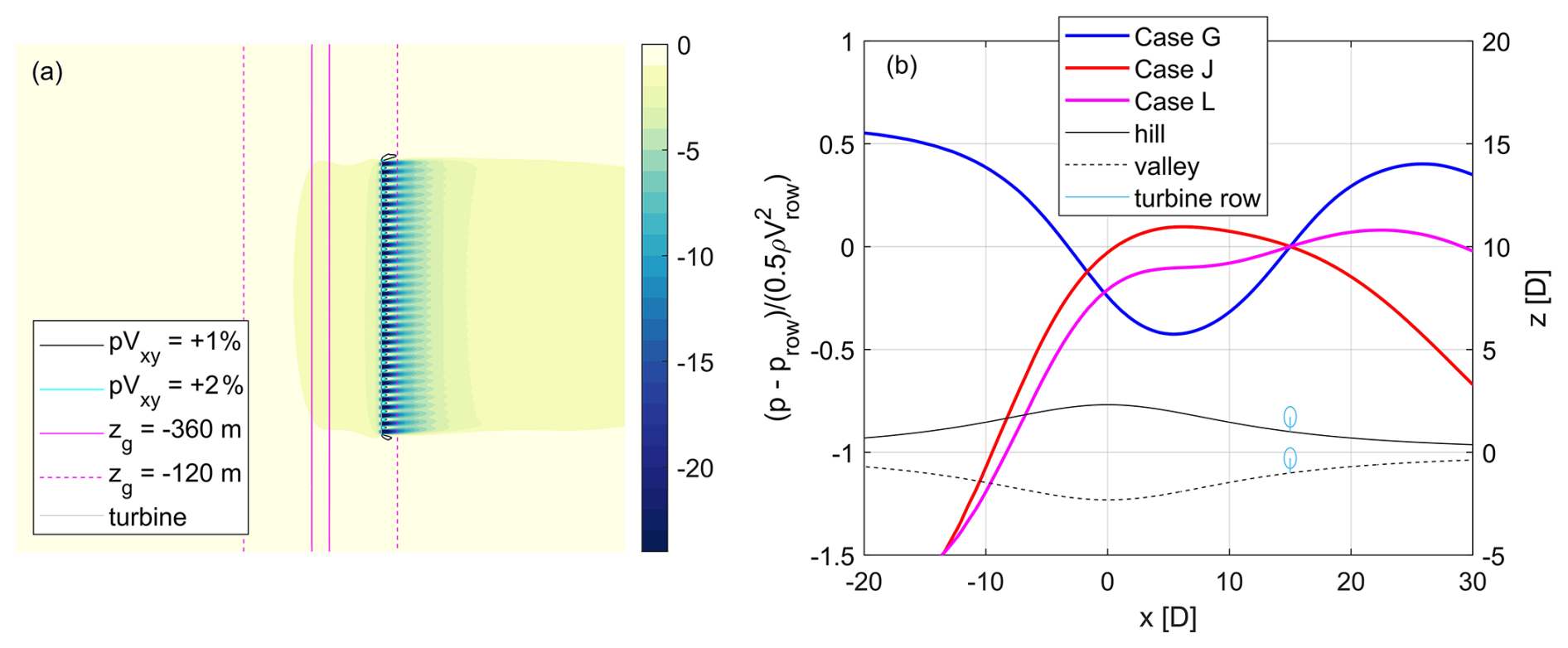
Figure 13 Top view of the percent change in wind speed relative to freestream at hub height for Case J (a) and freestream pressure coefficient along the terrain profiles at hub height at y = 0 m (b). The Case J (valley) pressure coefficient is in red, Case G (hill) is in blue, and Case L (valley) is magenta. The pressure coefficient is relative to conditions 15 D downstream of the hill crest and valley trough, the location of the turbine rows in the corresponding wind farm simulations. The thin black lines depict the valley and hill profiles.

We also analyzed two valley cases: Case J and Case L. The valley is a mirror image of the baseline hill, and the row is on the leeward side of the valley, 15 D downstream of the minimum elevation of −370 m. The altitude where the inversion starts, z_i, is 640 m. The main difference between the two cases is the prescribed geostrophic wind speed, which is 13.4 m s⁻¹ for Case J and 16.2 m s⁻¹ for Case L. Figure 13a shows the percent change in wind speed relative to freestream for Case J, and Fig. 13b shows the streamwise variation of freestream pressure at hub height along the terrain profiles for the two valley cases as well as for the hill case with the same z_i and turbine row location (Case G). The background streamwise pressure gradient near the turbine locations in Case J is clearly favorable, in sharp contrast to the hill case. This contributes to a huge difference in the wind farm wake (compare Fig. 13a with Fig. 9c). Again, we believe this difference in the wakes feeds back and contributes to significant differences in the effect of blockage upstream. This simple narrative is incomplete. In this instance, for example, other contributors to the differences in the wind farm wakes between the two cases include large differences in background turbulence levels as well as differences in blockage itself. Fully isolating causes and effects in such a fluid dynamic system is often not straightforward. Nevertheless, we can definitively state that the difference in blockage-related upstream slowdowns causes the large difference in the turbine interaction loss between the two cases: 15.6 % for the hill case and −1.8 % for this valley case, a turbine interaction gain. The faster flow in Case L responds differently to the terrain compared with Case J, resulting in a mild adverse pressure gradient in the background flow near the turbines (Fig. 13b) and a higher turbine interaction loss (+1.4 % vs. −1.8 %). The difference in freestream streamwise pressure gradients across the three cases also contributes to differences in the turbine efficiency (C_P), as discussed in Sect. 3.3.

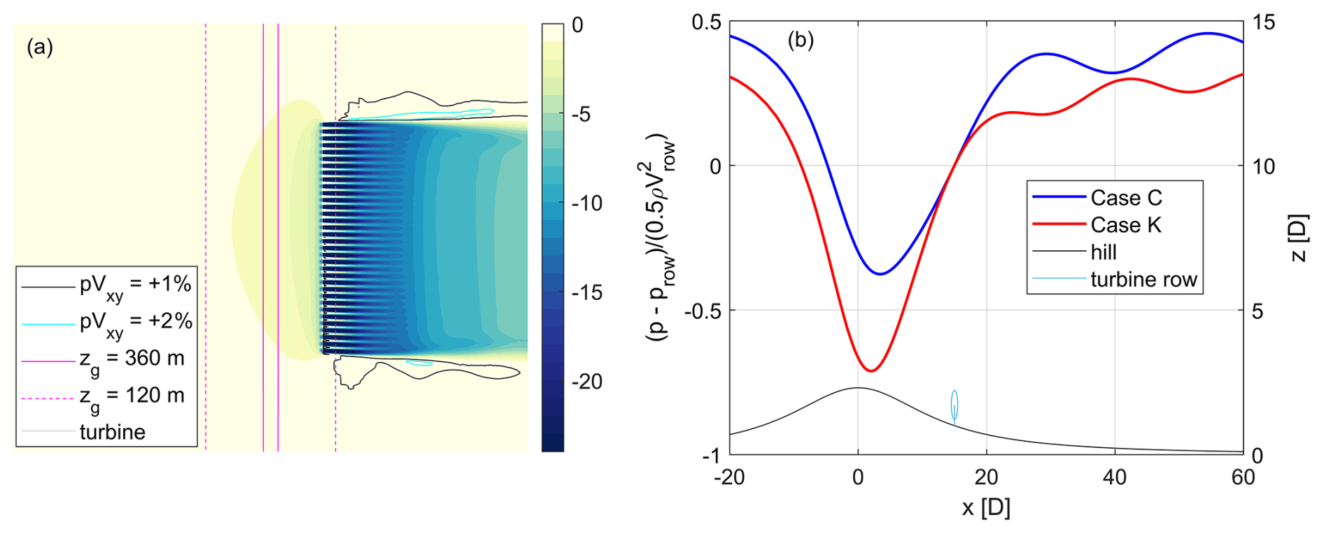
Figure 14 Top view of the percent change in wind speed relative to freestream at hub height for Case K (a) and freestream pressure coefficient along the hill profiles at hub height at y = 0 m (b). Case K is in red, Case C is in blue. The pressure coefficient is relative to conditions 15 D downstream of the hill crest, the location of the turbine rows in the corresponding wind farm simulations. The thin black line corresponds to the hill profile.

The effect of inflow wind speed on turbine interaction loss is also evident in the hill simulations. Case K is similar to Case C but runs with a lower geostrophic wind speed of 6.6 m s⁻¹ compared with 8.0 m s⁻¹ in Case C. This difference in wind speed results in a very different predicted loss (see Table 1). Figure 14a shows percent change in wind speed relative to freestream for Case K, and Fig. 14b shows the streamwise variation of freestream pressure along the hill for Case K and Case C. The phase and wavelength of the freestream gravity waves in the lee of the hill are clearly different between these two cases, with the lower wind speed case exhibiting hill-induced gravity waves with shorter wavelengths. The differences in the gravity waves contribute to differences in the streamwise variation of pressure in the lee of the hill. The streamwise pressure gradient at the turbine row is about the same between the two cases, but there is a greater pressure rise further downstream in Case C. This will contribute to a deeper wake. The fact that the wind farm wake in Case K is not as deep or thick compared to Case C may contribute to differences in the upstream blockage effect. In this way, hill-induced gravity waves indirectly contribute to upstream slowdowns. Gravity waves, and more generally the response of stratified flow to the hill and the turbines, may also affect these slowdowns more directly – as will be discussed later in this section.

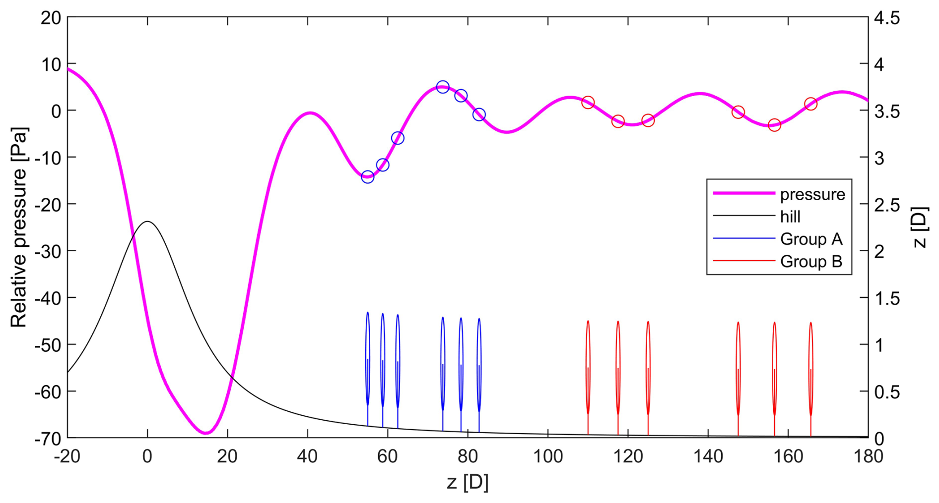
Figure 15 Freestream pressure variation for Case F. The locations of the six single-row wind farms in Group A (blue) and the six single-row wind farms in Group B (red) are shown relative to the location of the hill profile (black).

We ran additional simulations in order to further explore the various influences on turbine interaction loss in single-row wind farms. Twelve of the additional single-row analyses were run using the Case F inflow conditions and terrain. Gravity waves in this case induce significant streamwise pressure variations, even on the relatively flat terrain downstream of the hill. This can be seen in Fig. 15, which also shows the locations of the 12 additional single-row wind farms. The Group A wind farms correspond to locations where there are large local variations in the background pressure. The Group B wind farms are further downstream and generally correspond to locations where the local variations in pressure are smaller.

Also, two additional analyses were run on flat terrain, each with a lower inversion height (z_i = 590 m and z_i = 270 m). Finally, Case A and Case D were rerun with the buoyancy term in the vertical momentum equation zeroed out.

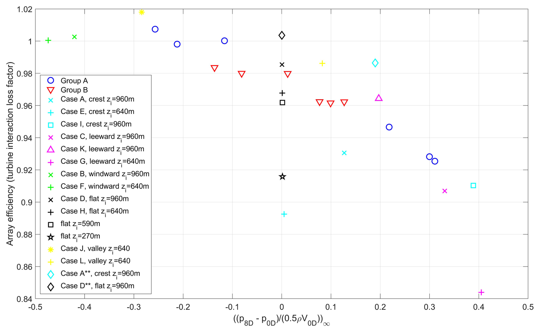
Figure 16 Array efficiency vs. freestream pressure coefficient for all single-row cases. The pressures are extracted from the freestream simulation at the turbine row location and 8 D downstream at hub height at y = 0 m. Cases without buoyancy are marked with two asterisks in the legend.

Plotting array efficiency vs. freestream pressure coefficient for all these cases provides insight into the physical influences on blockage-related upstream slowdowns. The pressure coefficient in Fig. 16 is equal to the pressure difference between the turbine row location and 8 D downstream, normalized by the dynamic pressure at the row location – with all values coming from the freestream simulation. There is a correlation between the freestream pressure coefficient and the array efficiency in Fig. 16. The correlation coefficient is −0.74, which translates to an r² of 0.54 for a linear regression of the data (r² is 0.61 when the two results without buoyancy are removed). The correlation does not materially improve when using different locations to calculate the pressure coefficient.

The trend across the flat-terrain cases (black symbols) is different from the overall trend in that there is significant variation in loss across the flat cases despite hardly any variation in the freestream pressure coefficient. As the inversion gets lower in the flat cases, the slowdown upstream of the single row becomes more pronounced and the array efficiency decreases, a trend consistent with the results reported in Bleeg and Montavon (2022). This finding suggests that there may be more influencing upstream slowdowns in single-row wind farms than just streamwise pressure variation in the background flow and its impact on wakes.

The trend across the flat cases may partially explain the trend across the crest cases (light blue), which also deviates from the overall trend. For example, in Case E, where the row is on the crest and z_i is 640 m, the freestream pressure drop between the row location and 8 D downstream is negligible, yet the upstream blockage effect is very strong (Fig. 9a), and the array efficiency is lower than the efficiencies in all but one of the other cases. Note that in this case the height of the inversion above the ground at the hill crest is comparable to the height of the inversion in the flat case with z_i = 270 m. The physical processes that contribute to the large upstream blockage effects in the flat case with z_i = 270 m may also contribute to the large blockage effects in Case E. These processes probably influence the blockage effects in the other cases too.

These physical processes likely relate to the response of stratified flow to an obstacle, which in this study is a row of turbines. A non-dimensional number relevant to upstream blockage effects is the local Froude number, which we define as follows:

$$\begin{array}{}\text{(4)}& \mathit{Fr}={\displaystyle \frac{{\stackrel{\mathrm{‾}}{u}}_{\text{BL}}}{\sqrt{g^{\prime }{h}_{\text{inv}}}}},\end{array}$$

where h_inv is the vertical distance between the ground and the altitude where the vertical gradient of the potential temperature is at a maximum. ${\stackrel{\mathrm{‾}}{u}}_{\text{BL}}$ is the average of the x component of velocity below h_inv. Finally, g^′ is the reduced gravity defined as $g^{\prime }=g\mathrm{\Delta }\mathit{\theta }/{\mathit{\theta }}_{\mathrm{0}}$, where g is the acceleration due to gravity (9.81 m s⁻²), Δθ is the change in potential temperature across the inversion (5 K), and θ₀ is the reference potential temperature (286 K). The inputs to Eq. (4) come from the freestream simulations.

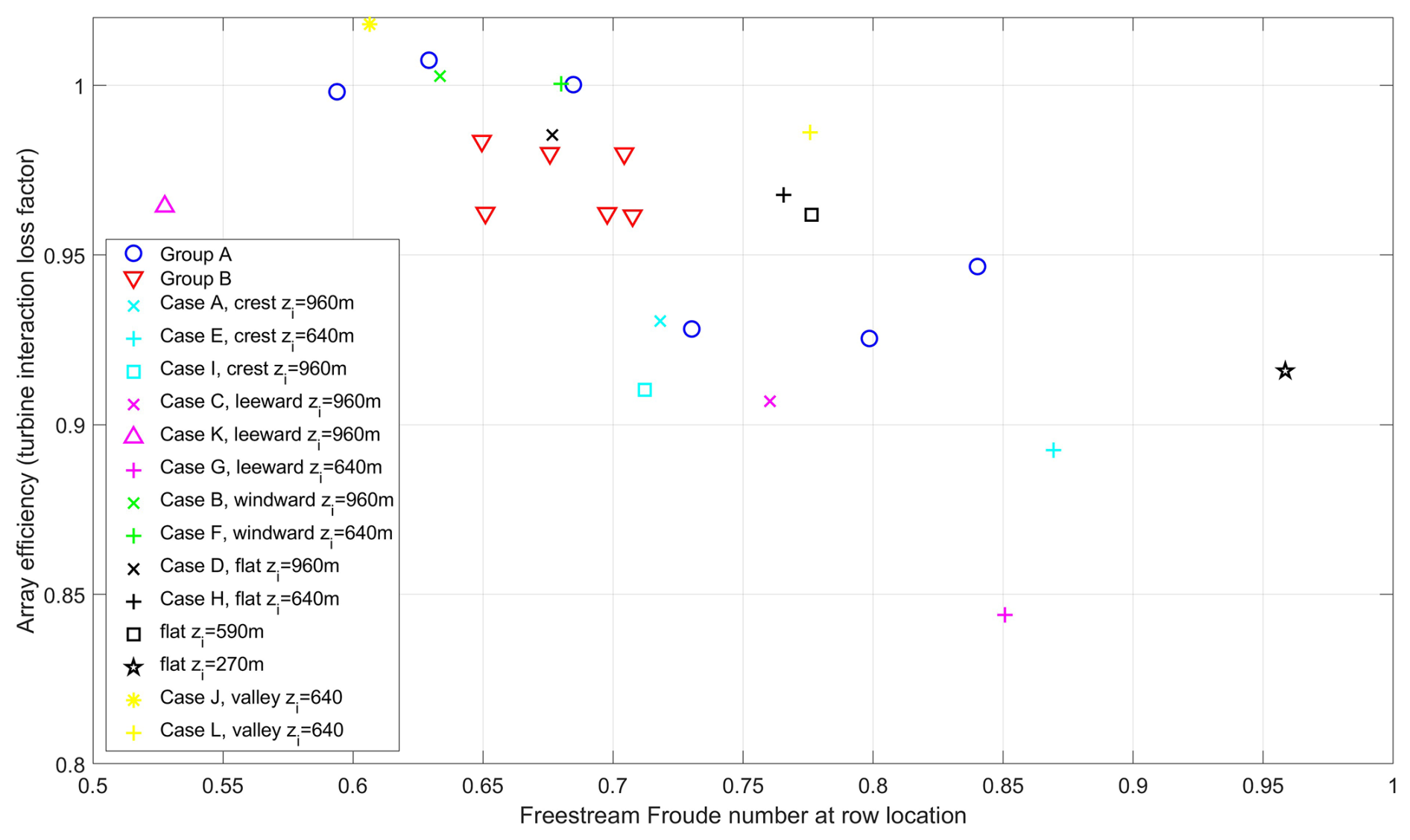
Figure 17 Array efficiency vs. local freestream Froude number for all single-row cases with buoyancy in the momentum equation.

The Froude number as defined above represents the ratio of the local wind speed to the wave speed along the inversion. As the freestream local Froude number increases and approaches 1.0 in these simulations, the upstream effect of a turbine row introduced to the flow generally increases, causing the efficiency of the row to decrease. This can be seen in Fig. 17, which shows array efficiency vs. local Froude number for all the cases except for the two cases with buoyancy zeroed out of the vertical momentum equation. There is a strong correlation between Froude number and single-row efficiency for the flat cases (black symbols). Across the other cases, a correlation is still present, but it is not as strong. The correlation coefficient, r, across all cases is −0.68. A multi-variable linear regression of the wind farm efficiency data with local Froude number and pressure coefficient as independent variables yields an r² value of 0.76, which is significantly higher than the r² values from separate single-variable linear regressions of the efficiency data (r² is 0.47 when using local Froude number and 0.61 when using pressure coefficient). The efficiency trends may correlate better with different or additional independent variables. For example, vertical shear likely influences η as it did in Bleeg and Montavon (2022). Turbulence might also affect blockage and η via its influence on wake recovery: the correlation coefficient between freestream turbulence intensity and η for these cases is +0.58, with r² = 0.33 (if the two zero-buoyancy cases are included, the correlation coefficient is +0.51, with r² = 0.26). In any case, the inviscid response of the stratified flow to terrain and the turbine row appears to have a significant influence on the upstream blockage effect in these simulations. Underlining this point, if we turn off the buoyancy in the vertical momentum equation (diamond symbols in Fig. 16), the upstream blockage effect decreases and the row efficiency increases, especially for Case A, where the row is on the hill crest. That said, even with the buoyancy turned off, blockage effects and array efficiency are still sensitive to terrain (the η difference between the two zero-buoyancy cases is 1.65 %). So while buoyancy is a primary contributor to the effect of terrain on blockage in this study, it clearly is not the only contributor.

3.3 Turbine performance

Not only can terrain influence wind farm efficiency, but it can also affect turbine efficiency. The nominal C_P level for the simulated turbine is 0.445 when the hub-height freestream wind speed is between 6.1 and 9.6 m s⁻¹ (Fig. 2). Even though the simulated turbines in this study operate within this wind speed range, the C_P values derived from the results using Eq. (3) can depart significantly from 0.445. In Table 1, the C_P values vary between 0.408 and 0.477.

Turbine power is traditionally seen as a function of freestream conditions, but in fact it is more directly a function of the wind conditions at the rotor face during turbine operation. It is the conditions at the rotor face that determine the loads on the blades and in turn the rotor thrust and torque. The actuator disks in this study behave similarly: thrust and torque are functions of wind conditions at the disk when the actuator disk is on. The power coefficient, C_P, is the ratio between the power of a solitary turbine and the flux of kinetic energy passing through the rotor area when the turbine is not there. C_P varies substantially across the different cases in this study, implying that terrain can change the relationship between the freestream conditions and the conditions at the rotor disk. More specifically, it can affect induction factor. If terrain leads to an increase in the induction factor, the wind speed at the turbine rotor face decreases, decreasing power relative to the freestream kinetic energy flux. In other words, for a given turbine model, an increase in induction factor reduces C_P.

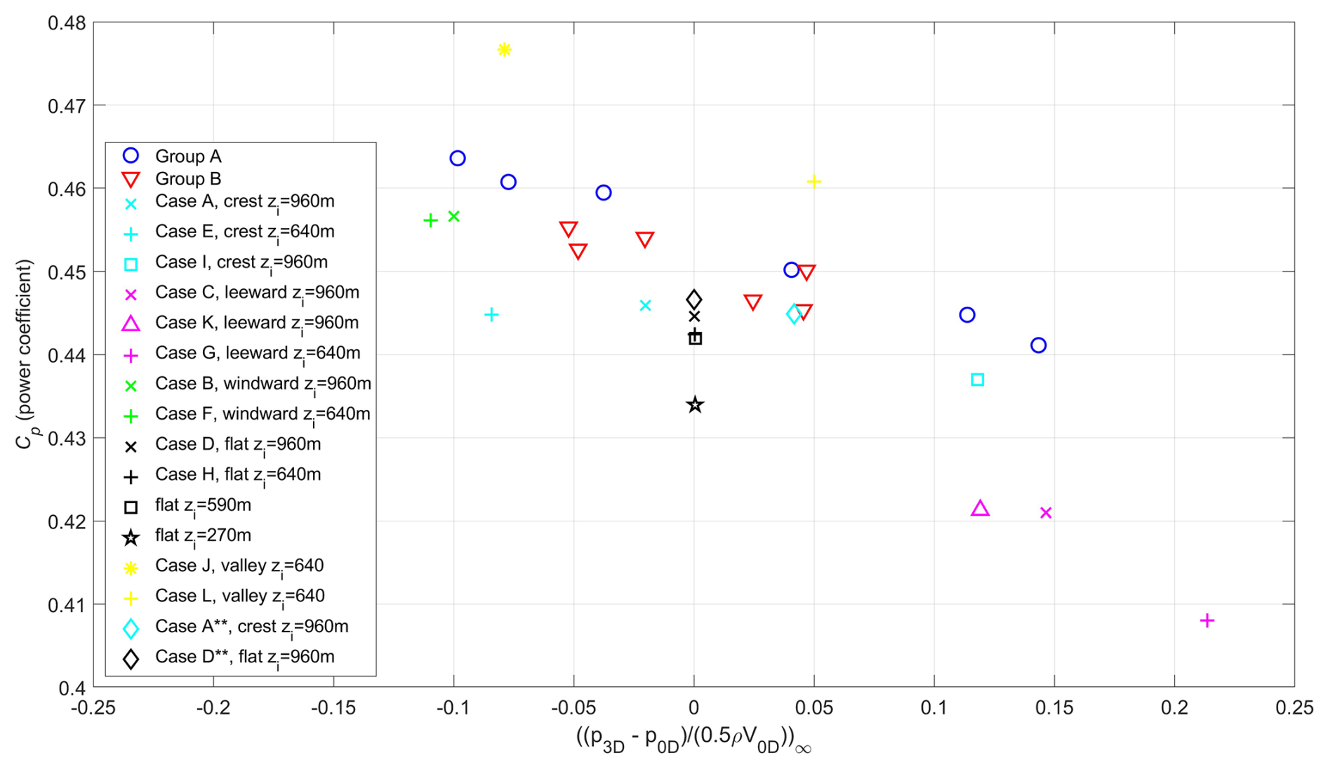
Figure 18 Individual turbine efficiency (C_P) vs. freestream pressure coefficient. The pressures are extracted from the freestream simulation at the turbine location and 3 D downstream at hub height at y = 0 m. Power is extracted from isolated turbine simulations. Cases without buoyancy are marked with two asterisks in the legend.

Variations in induction factor and power coefficient are perhaps more commonly associated with wind turbine design changes. Here, rather, we claim that for a given turbine design, external factors such as terrain-induced streamwise pressure variations can affect induction factor and thereby C_P. Figure 18 plots C_P against freestream pressure coefficient for the cases in this study. This time the pressure coefficient is between the turbine row locations and locations 3 D downstream (instead of 8 D). There is a correlation between C_P and the freestream pressure coefficient (r = −0.78), suggesting that streamwise variation in the background freestream pressure across the near wake may influence C_P. We believe the mechanism is similar to that described in the previous section and in Revaz and Porté-Agel (2024): streamwise variations in the background pressure affects the depth and size of the near wake and in turn the amount by which oncoming flow deflects relative to freestream conditions. The amount by which the oncoming flow deflects directly connects with induction and thereby C_P. As discussed in the Introduction, many other researchers have identified a connection between streamwise variation in the background (freestream) flow and turbine efficiency, using both simulations (Troldborg et al., 2022; Zengler et al., 2024; Revaz and Porté-Agel, 2024) and wind tunnel experiments (Dar et al., 2023).

The factors influencing C_P in this study do not appear to be limited to terrain-induced streamwise pressure variations. Within narrow bands of freestream pressure coefficient there are significant differences in C_P in Fig. 18. Across the flat cases, where pressure coefficient deviates little from zero, turbine efficiency decreases as z_i decreases, though not as dramatically as the wind farm efficiency in Fig. 16. It is possible that stratification above the boundary layer affects turbine blockage and contributes to the C_P trend in the flat cases and other cases. But there are likely other contributors: Dar et al. (2023) and Revaz and Porté-Agel (2024) also show clear but imperfect correlations between C_P and streamwise pressure variation, but in these studies, the other contributors to C_P variation cannot be related to stable stratification, as the flows are purely neutral, with no buoyancy.

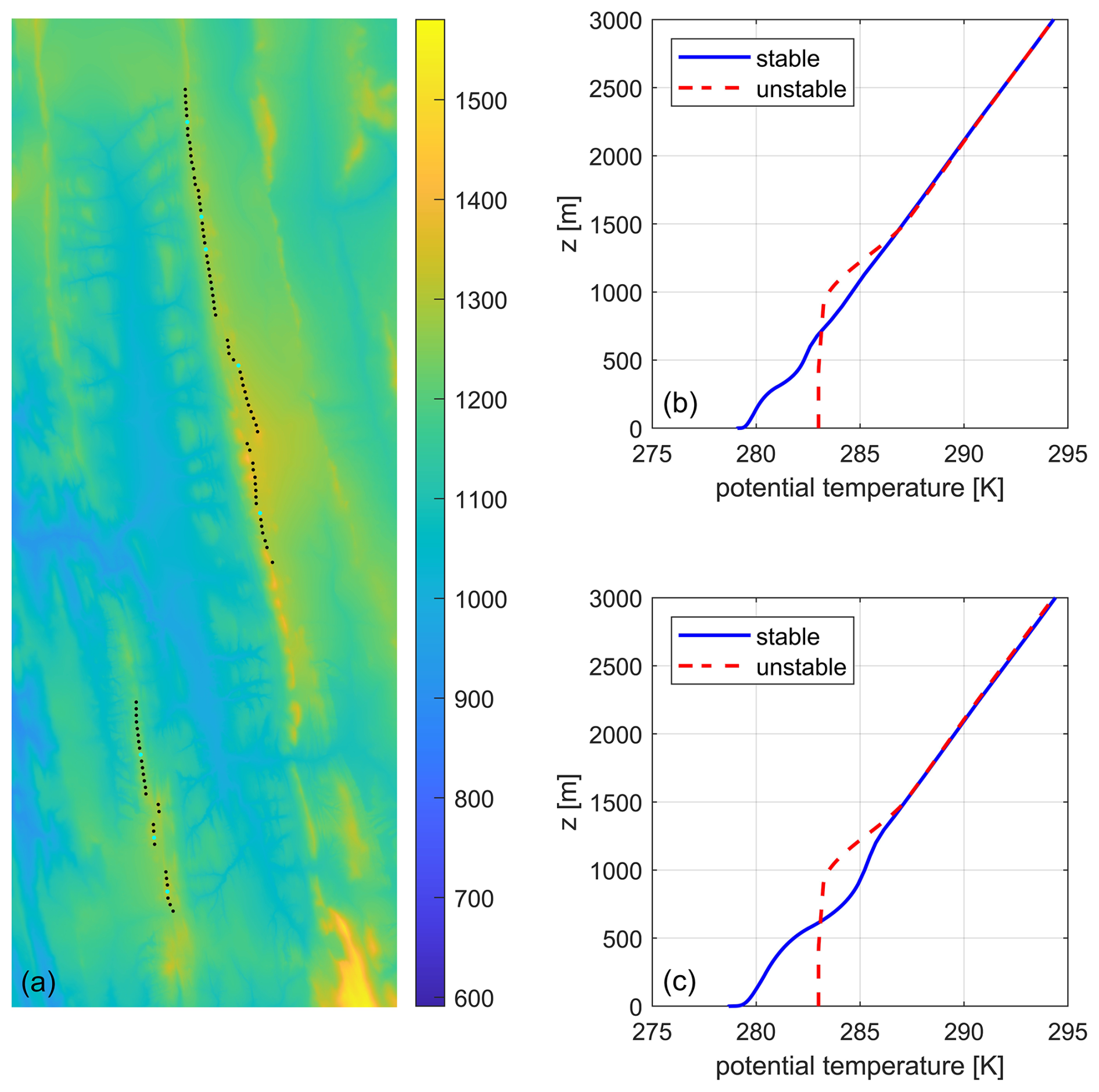
Figure 19 Elevation map and turbine layout (a), inflow potential temperature profiles for the real-terrain simulations (b), and inflow potential temperature profiles for the flat-terrain simulations (c). Light-blue dots on the map represent turbines that were also simulated in isolation in both unstable and stable conditions.

3.4 A real wind farm

The results presented so far have been from simulations of notional wind farms in conventionally neutral boundary layers on idealized terrain. The results in this subsection are from simulations of a real wind farm with inflow atmospheric conditions derived from the output of a mesoscale model. The subject wind farm has 94 modern wind turbines organized in rows atop ridgelines, as depicted in the elevation map in Fig. 19. The spacing between turbines is tight, with hub-to-hub distances as low as 1.5 D. The north, south, east, and west domain boundaries are at least 16 km from the turbines, and the top boundary is 17 km above the maximum ground elevation in the simulation.

Results from the Weather Research and Forecasting (WRF) model run with the Mellor–Yamada–Jancic (MYJ) boundary layer scheme over a full year were used to inform the RANS inflow boundary conditions. We started with a time series of vertical profiles extracted from the WRF output at a location approximately coincident with the east boundary of the RANS model. We then filtered the time series of profiles for eastern flows and divided the remaining records into two batches – one corresponding to unstable surface conditions and the other corresponding to stable surface conditions. For each batch of records, we derived a single set of profiles (potential temperature, velocity, and turbulence quantities) intended to represent the average conditions in the batch. The inflow potential temperature profiles for the RANS simulations are shown in Fig. 19b and c. The profiles in Fig. 19b were used in the simulations of the wind farm on real terrain. The profiles in Fig. 19c were used in the simulations of the wind farm layout on flat terrain. The inflow wind speed levels were set such that the turbines across all the cases experience similar wind speeds. This can be done while maintaining the same potential temperature profiles for the flat and real terrain cases when the simulated boundary layer is unstable; however, in our approach to simulating stable boundary layers (Bleeg et al., 2015a), the differences in the inflow wind speeds between the flat and real terrain cases necessitate somewhat different potential temperature profiles.

The unstable potential temperature profile does not include a superadiabatic lapse rate in the surface layer. We do this to avoid the occurrence of thermal convections in the solution, as convective structures resolved by a RANS model would likely be spurious. We instead simulate the unstable boundary layer as a conventionally neutral boundary layer but with additional turbulence source terms designed to represent the impact of convections on turbulence, and in turn the mean flow. The source terms are based on similarity theory (Vulfson and Nikolaev, 2022), with the main inputs being ground heat flux and the height of the boundary layer (158 W m⁻² and 1000 m in this case). Bleeg et al. (2023) provide more information on this approach to simulating unstable boundary layers in RANS.

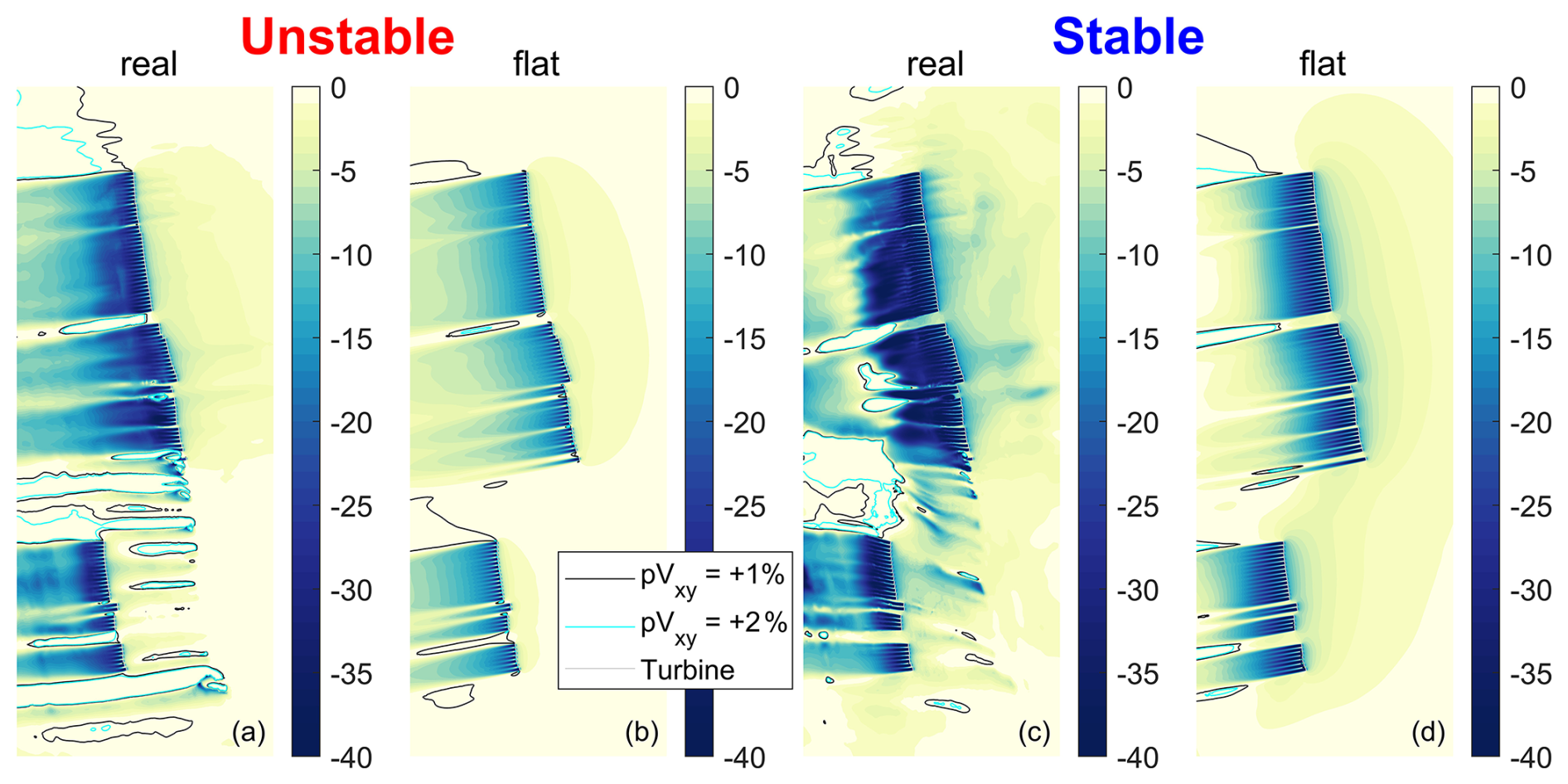
Figure 20 Top view of the percent change in wind speed relative to freestream at hub height for the simulation of the unstable boundary layer in real terrain (a), the unstable boundary layer in flat terrain (b), the stable boundary layer in real terrain (c), and the stable boundary layer in flat terrain (d).

The average freestream hub-height wind speed across the turbines in all these simulations is approximately 8 m s⁻¹. The average wind direction is 80°. Figure 20 depicts the results from these simulations.

In the real-terrain results (Fig. 20a, c), the wakes downstream of the wind farm are generally deeper at hub height than the wakes in the flat terrain results (Fig. 20b, d). The blockage-related upstream slowdowns in real terrain are also more pronounced, with the slowdowns greater in the simulations of the stable boundary layer than the unstable boundary layer for both real and flat terrain. The loss trends between the cases reflect the difference in upstream blockage effects. In both unstable and stable conditions, the turbine interaction loss is about 4 % greater in real terrain than in flat terrain for the simulated conditions. In unstable conditions, the predicted loss is 5.3 % in real terrain and 0.9 % in flat terrain. In stable conditions, the loss is 16.5 % in real terrain and 12.4 % in flat terrain. Note that the loss predictions in this paper correspond to the simulated conditions only; if the turbine interaction analysis considered the full range of atmospheric conditions at this wind farm, particularly the wind speed distribution, the predicted blockage-related losses would be much lower.

It is somewhat less straightforward to assess the effect of terrain on turbine efficiency in this case compared with the idealized cases. This is due to the variability of the terrain in combination with the fact that, unlike the C_P curve in Fig. 2, the C_P curve of a real wind turbine is not constant over a wide range of wind speeds. That said, the maximum variation along the nominal C_P curve between 7 and 9 m s⁻¹ is just 1 %. In the following discussion, this operating range is labeled the “nearly flat” part of the nominal C_P curve (again, the nominal C_P curve informs the U_disk-based turbine performance look-up tables used in the simulations). We simulated 8 of the 94 turbines in isolation; these turbines, which are spread across the wind farm, are highlighted with light-blue dots in Fig. 19a. When simulated on the real terrain, whether in the stable or unstable conditions, 6 of the 8 solitary turbines end up on the nearly flat part of the nominal C_P curve. In stable conditions, the two northernmost isolated turbines are outside the nearly flat range, and in unstable conditions, the northernmost isolated turbine in each of the two rows is outside this range. When simulated on flat terrain, all the isolated turbines operate on the nearly flat part of the nominal C_P curve. If we calculate C_P from the isolated and freestream simulations using Eq. (3) and limit the calculation to turbines operating on the nearly flat part of the nominal C_P curve, the average C_P for the turbines simulated in real terrain is more than 4 % lower than the average C_P of the turbines simulated on flat ground – specifically, 4.4 % lower in unstable conditions and 4.5 % lower in stable conditions. As with wind farm efficiency, the average effect of terrain on turbine efficiency will be much lower when aggregated over the full range of wind speeds.

In this subsection, simulations of a real wind farm with characteristics similar to the idealized wind farms in Sect. 3.2 – but using site-specific inflow conditions instead of conventionally neutral boundary layers – yield results consistent with the findings derived from the idealized wind farms with respect to the effect of terrain on wakes, blockage, and efficiency. It is not known from these results the extent to which the findings apply to onshore wind farms in general. To understand this better, future work could involve simulating other types of terrain and wind farm layouts.

4 Discussion

Terrain influences wake and blockage effects at wind farm scale and turbine scale according to the RANS results presented in Sect. 3. In this section, we discuss the practical implications of these findings as well as how much weight one should place on the findings given limitations in the modeling and the scope of the investigation. We also discuss the types of field observations that could improve our understanding of the effect of terrain on wakes and blockage.

4.1 Practical implications

The influence of terrain on wakes and blockage may have significant implications for wind farm energy yield. According to the results of this RANS-based study, terrain can influence not only array efficiency (η) but also turbine efficiency (C_P). Further, there might be a correlation between the effect of terrain on η and the effect of terrain on C_P. In the single-row wind farms in this study, the correlation coefficient between η and C_P is 0.81 (ignoring the two cases without buoyancy).

Take for example Case C, a single row on the leeward side of the hill with z_i = 960 m. In this case, the turbines collectively produce 9.31 % less power than they would if each one were simulated in isolation. By comparison, the turbine interaction loss, L, in the corresponding flat-terrain analysis, Case D, is 1.46 %. Thus, the wind farm turbines in Case C are 7.85 % less efficient relative to isolated operation than the turbines in Case D. On top of that, the isolated turbines in Case C are also less efficient, with a C_P of 0.421 compared to 0.444 in Case D, a difference of 5.81 %. As a result, the overall energy conversion efficiency of the wind farm, C_P,WF, is 12.8 % less in Case C (0.382) than in Case D (0.438).

Current industry practices for estimating the energy yield of a planned wind farm largely neglect the effect of terrain on wakes and blockage, as well as the related effect terrain has on wind farm efficiency and individual turbine efficiency. This could lead to material prediction errors, which would contribute to uncertainty in energy yield predictions. These errors may also result in wind farms that are less productive than they otherwise would be if terrain effects were more fully accounted for during the design of the wind farm.

Mitigating this risk requires flow modeling that captures the key fluid dynamic elements contributing to the influence of terrain on wakes and blockage. Most commonly used engineering models are able to partially account for terrain-induced turbulence and its impact on wakes; however, at present these models are not able to simulate terrain-induced inviscid effects, which can substantially affect turbine interaction loss. Terrain-induced streamwise pressure gradients can have a large impact on wake development, which in turn influences upstream blockage effects. The inviscid response of stratified flow to the terrain and wind farm further modifies blockage effects. Completing the interlinkage, blockage effects influence wake development (Lanzilao and Meyers, 2024; Ndindayino et al., 2025). In other words, terrain affects wakes, which affect blockage; terrain also directly influences blockage, which affects wakes. It is a tightly coupled fluid dynamic system, and the approach used to model it should aim to reflect this overarching aspect of the flow.

4.2 Limitations

How seriously one should take these conclusions depends in no small part on the reliability and the representativeness of the simulations behind them. With respect to real-world representativeness, the effect of terrain on wakes and blockage may be generally larger in idealized quasi-2D terrain than in real terrain. The effect may also be larger, or at least different, for wind farms organized in rows with tight spacing as compared to other types of turbine layouts. The simulated atmospheric conditions also raise questions of representativeness: the effect of terrain on stratified flow is very sensitive to the simulated atmospheric conditions, particularly the potential temperature profile; if the atmospheric conditions simulated in an analysis of a particular wind farm are not representative of the actual site conditions, it could result in substantial errors in the prediction of the impact of terrain on wake and blockage effects.

With respect to the reliability of the simulations, the RANS model used in this study has shown good agreement with field observations related to blockage and wakes at many wind farms, including three with elevation variation on the order of what is simulated in this study (these three are internal validations not reported in the references provided in Sect. 2.1). Even so, there are reasons to question the near-wake predictions. Simulations with actuator disks cannot capture some of the important flow features in a near wake, like hub and tip vortices, and internal validation indicates that the near wakes simulated with this RANS model generally diffuse too rapidly relative to field observations. The effect of terrain-induced streamwise pressure gradients on the near wake of an individual turbine is proposed to be central to the impact of terrain on turbine efficiency. Given these facts, there is enhanced risk that the predicted turbine efficiency trends are inconsistent with what would occur in the field. That said, several other recent studies cited herein, including a wind tunnel experiment, have yielded similar trends.

4.3 Field observations wanted

Relevant field observations could improve our understanding of the impact of terrain on wakes and blockage as well as our understanding of the reliability of related flow modeling. Wind speed measurements taken just upstream of a wind farm for sufficiently long periods before and after the wind farm starts operating could help in assessing the effect of terrain on wind farm blockage. As described in Bleeg et al. (2018), an analysis of the data can reveal the degree to which the wind speed upstream of the wind farm changes relative to a reference wind speed time series due to the presence of the wind farm. Separately, turbine power data from a wind farm located in terrain where there are marked streamwise variation in the background wind speed could help in the assessment of the effect of terrain on wakes.

However, it is difficult to isolate the impact of terrain on field observations related to blockage and wakes. Unlike in a wind tunnel or a simulation, it is not reasonably possible in the field to obtain back-to-back measurements of a similar wind farm in flat terrain. A way forward could be to compare the measurements with simulations of the wind farm layout on the real terrain and on flat terrain. The comparison could provide insight into both the reliability of the simulations and the degree to which terrain is affecting blockage and wake effects at the subject wind farm.

As for the effect of terrain on turbine efficiency, a type of measurement commonly used in the wind industry may be relevant. The theory promoted here, and elsewhere, is that terrain can affect induction and in turn C_P. This terrain effect, if real, is likely reflected in standard turbine power performance measurements (PPMs), which involve concurrent measurements of turbine power and upstream wind speed. The IEC standard for turbine PPM, IEC 61400-12 (2022), requires that the wind speed measurement take place 2 to 4 rotor diameters upstream of the test turbine, where the effect of turbine induction is small (Medici et al., 2011). Thus, any impact of terrain on induction should have less of an impact on the measured wind speed than on the wind speed at the rotor face. Therefore, if terrain has an impact on C_P, it should be at least partly captured in the PPM. That said, even if the effect of terrain is captured in the measurements, it will not be straightforward to isolate the effect. An assessment of many measured C_P curves from a single turbine model across a variety of topographies may help – especially if done in conjunction with simulations with and without the real terrain. Still, there are many confounding factors that can directly influence turbine power performance – including flow inclination, shear, and turbulence, all of which are sensitive to terrain – and it may be difficult to truly isolate from the measurements the effect of terrain on induction and in turn turbine efficiency.

5 Conclusions

We simulated 35 different combinations of wind farm layout, terrain, and inflow atmospheric conditions using RANS. The wind farms were organized in one or two rows of closely spaced turbines. The terrain in nearly all cases was idealized, either quasi-2D or flat, and the inflow boundary layers in these cases were neutral, with overlying thermal stratification. The few remaining cases correspond to a real wind farm with characteristics similar to some of the idealized wind farms but simulated in a stable or an unstable boundary layer. Terrain had a pronounced influence on wake and blockage effects in the simulation results. Further, the RANS-predicted wind farm efficiencies and turbine efficiencies in terrain, whether idealized or real, departed markedly from back-to-back RANS predictions on flat ground.

Hill-induced streamwise pressure gradients can have a large influence on wake development, and we propose, based on the results of this study, that this effect can feed back to influence upstream slowdowns related to blockage. Further analysis of the results, including an assessment of local Froude number, suggests that the inviscid response of stratified flow to a wind farm in terrain can additionally affect wind farm blockage – in a way related to but distinct from its effect on blockage via terrain-induced pressure gradients as they pertain to wake recovery.

This work differs in a few ways from earlier studies on the combination of terrain and wind turbines. Perhaps most notably, we consider the effect of terrain on both wakes and blockage. And whereas previous studies were limited to purely neutral flows, with no buoyancy, this study includes the effects of thermal stratification, which can significantly modify flow over terrain and its response to the presence of a wind farm. Finally, by virtue of simulating full wind farms, we directly connect the impact of terrain to wind farm efficiency.

That said, this study is not without its own limitations. From the terrain and the wind farm layouts to the atmosphere, the simulated conditions are mostly idealized. The simulations of an existing wind farm mitigate this concern somewhat in that the results are reasonably consistent with the findings from the idealized wind farms. Nevertheless, the general applicability of some of these findings can be fairly questioned due to the limited range of layout types and terrain types investigated. An analysis of a broader range of wind farms could help provide a more comprehensive understanding of the impact of terrain on wakes and blockage. Further, relevant, publicly available field observations could help improve confidence in the model and the study findings.

In the meantime, between this study and those that came before, there appears to be enough evidence to make the following claim: at proposed wind farm sites where terrain induces significant streamwise variation in wind speed, energy yield prediction approaches that do not capture the effect of terrain on wakes and blockage are at increased risk of elevated prediction errors. This could materially increase uncertainty in the energy yield predictions and perhaps even lead to less efficient wind farm layout designs.

Appendix A

We conducted control volume analyses (CVAs) to parse and better understand the various contributors to wake recovery between the first and second rows in the flat, hill windward, and hill leeward RANS results discussed in Sect. 3.1. The control volume for the hill leeward case is depicted in Fig. A1. In each of the cases, the control volume coincides with the rotor layer, from 35 $\mathrm{m}\mathrm{a}.\mathrm{g}.\mathrm{l}.$ (above ground level) to 195 $\mathrm{m}\mathrm{a}.\mathrm{g}.\mathrm{l}.$ The western surface of the control volume is 2.5 D downstream of the first row, and the eastern surface is 2.5 D upstream of the second row. These x locations were chosen to avoid, largely, the strong pressure variations in the near wakes and induction zones of the turbines. The northern surface is 3.0 D north of the hub of the northernmost turbine in the wind farm, and the southern surface is 3.0 D south of the wind farm.

The CVA focuses on the conservation of the x component of momentum. Since the wind direction through the control volume is very close to 270°, consideration of the y component of momentum in the CVA is not expected to significantly affect this assessment of the contributors to wake recovery. The contributors to the x component of momentum in the control volume are depicted in Fig. A1 and are as follows. M_x,i refers to the advection of the x component of momentum through surface i, where i is either W, E, N, S, B, or T (west, east, north, south, bottom, or top). F_P,i is the x component of the pressure force on surface i. F_P,T and F_P,B are zero in the flat case. F_C is the x component of the Coriolis force acting on the control volume. In this CVA, the geostrophic pressure field is included in the pressure forces, not the Coriolis force. Finally, F_S,i is the x component of the resultant force due to Reynolds stresses (turbulent fluxes) acting on surface i; these terms represent the turbulent transport of momentum, also referred to as the turbulent diffusion of momentum. The equation for the conservation of momentum in the control volume (V) is as follows:

$$\begin{array}{}\text{(A1)}& \begin{array}{rl}\int {\displaystyle \frac{\partial \left(\mathit{\rho }u\right)}{\partial t}}\mathrm{d}V=& (M_{x,\mathrm{W}}-M_{x,\mathrm{E}})+(M_{x,\mathrm{S}}-M_{x,\mathrm{N}})\\ & +(M_{x,\mathrm{B}}-M_{x,\mathrm{T}})+F_{\mathrm{P}}+F_{\mathrm{C}}\\ & +(F_{\mathrm{S},\mathrm{W}}+F_{\mathrm{S},\mathrm{E}}+F_{\mathrm{S},\mathrm{S}}+F_{\mathrm{S},\mathrm{N}}\\ & +F_{\mathrm{S},\mathrm{B}}+F_{\mathrm{S},\mathrm{T}}).\end{array}\end{array}$$

Here, F_P is the x component of the of the resultant sum of the pressure forces on the control volume, ρ is the density, and u is the x component of velocity. Since the simulations are steady state, the time rate of change of momentum is zero:

$$\begin{array}{}\text{(A2)}& \begin{array}{rl}\mathrm{0}=& (M_{x,\mathrm{W}}-M_{x,\mathrm{E}})+(M_{x,\mathrm{S}}-M_{x,\mathrm{N}})+(M_{x,\mathrm{B}}-M_{x,\mathrm{T}})\\ & +F_{\mathrm{P}}+F_{\mathrm{C}}\\ & +(F_{\mathrm{S},\mathrm{W}}+F_{\mathrm{S},\mathrm{E}}+F_{\mathrm{S},\mathrm{S}}+F_{\mathrm{S},\mathrm{N}}\\ & +F_{\mathrm{S},\mathrm{B}}+F_{\mathrm{S},\mathrm{T}}).\end{array}\end{array}$$

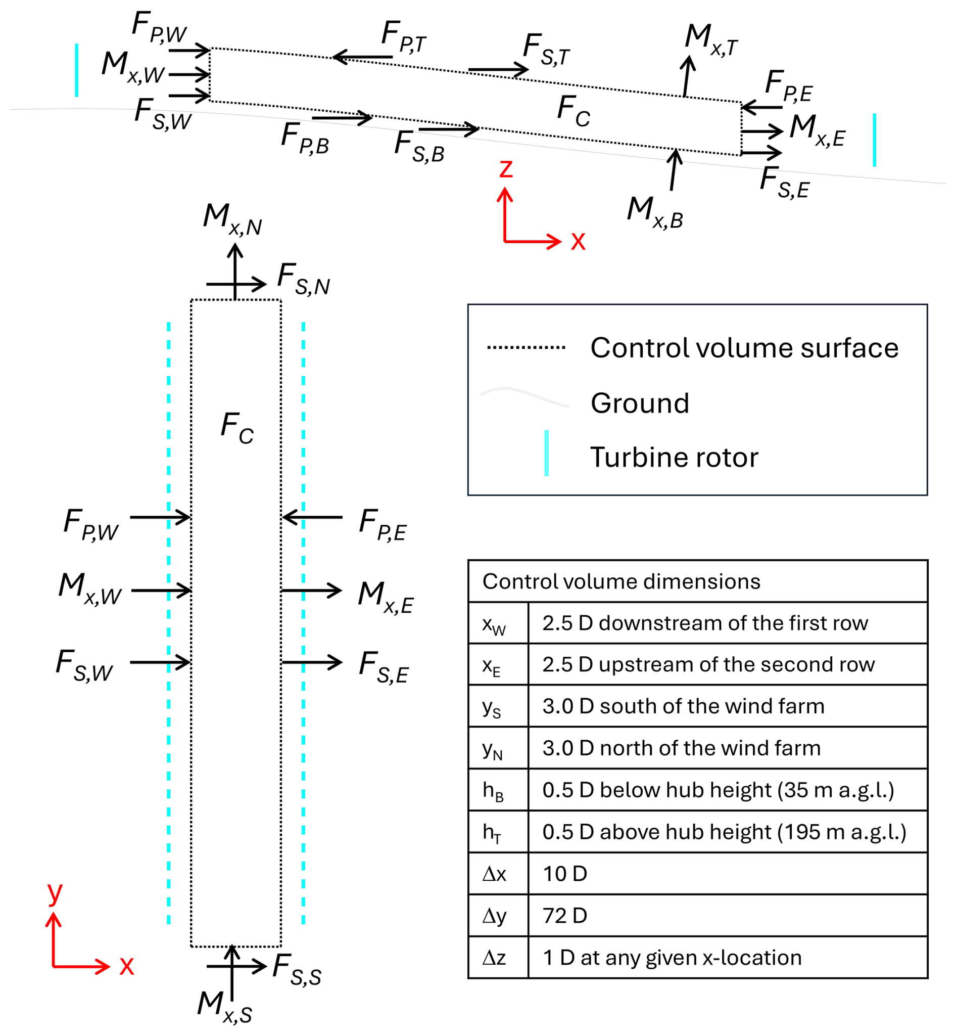
Figure A1 Diagram of the control volume analysis for the two-row cases in Sect. 3.1. The side view, on an xz plane, is from the hill leeward case.

Moving the first bracketed term over to the left-hand side, we get an equation for the increase in the advection of the x component of momentum from the west surface to the east surface – from 2.5 D downstream of the first row of turbines to 2.5 D upstream of the second row of turbines:

$$\begin{array}{}\text{(A3)}& \begin{array}{rl}{M}_{x,\mathrm{E}}-M_{x,\mathrm{W}}=& (M_{x,\mathrm{S}}-M_{x,\mathrm{N}})+(M_{x,\mathrm{B}}-M_{x,\mathrm{T}})\\ & +F_{\mathrm{P}}+F_{\mathrm{C}}+(F_{\mathrm{S},\mathrm{W}}+F_{\mathrm{S},\mathrm{E}}+F_{\mathrm{S},\mathrm{S}}\\ & +F_{\mathrm{S},\mathrm{N}}+F_{\mathrm{S},\mathrm{B}}+F_{\mathrm{S},\mathrm{T}}).\end{array}\end{array}$$

We can combine some of the advection terms to simplify the presentation of the results: $M_{x,\mathrm{S}-\mathrm{N}}=M_{x,\mathrm{S}}-M_{x,\mathrm{N}}$; $M_{x,\mathrm{B}-\mathrm{T}}=M_{x,\mathrm{B}}-M_{x,\mathrm{T}}$; and $M_{x,\mathrm{E}-\mathrm{W}}=M_{x,\mathrm{E}}-M_{x,\mathrm{W}}$. $M_{x,\mathrm{S}-\mathrm{N}}$ is the net lateral advection of the x component of momentum into the control volume. $M_{x,\mathrm{B}-\mathrm{T}}$ is the net advection of the x component of momentum through the bottom and top surfaces. And again, $M_{x,\mathrm{E}-\mathrm{W}}$ is the increase in the advection of the x component of momentum from the west to the east surface.

$$\begin{array}{}\text{(A4)}& \begin{array}{rl}{M}_{x,\mathrm{E}-\mathrm{W}}=& M_{x,\mathrm{S}-\mathrm{N}}+M_{x,\mathrm{B}-\mathrm{T}}+F_{\mathrm{P}}+F_{\mathrm{C}}+(F_{\mathrm{S},\mathrm{W}}\\ & +F_{\mathrm{S},\mathrm{E}}+F_{\mathrm{S},\mathrm{S}}+F_{\mathrm{S},\mathrm{N}}+F_{\mathrm{S},\mathrm{B}}+F_{\mathrm{S},\mathrm{T}})\end{array}\end{array}$$

Table A1 Definitions for the terms in Eq. (A4).

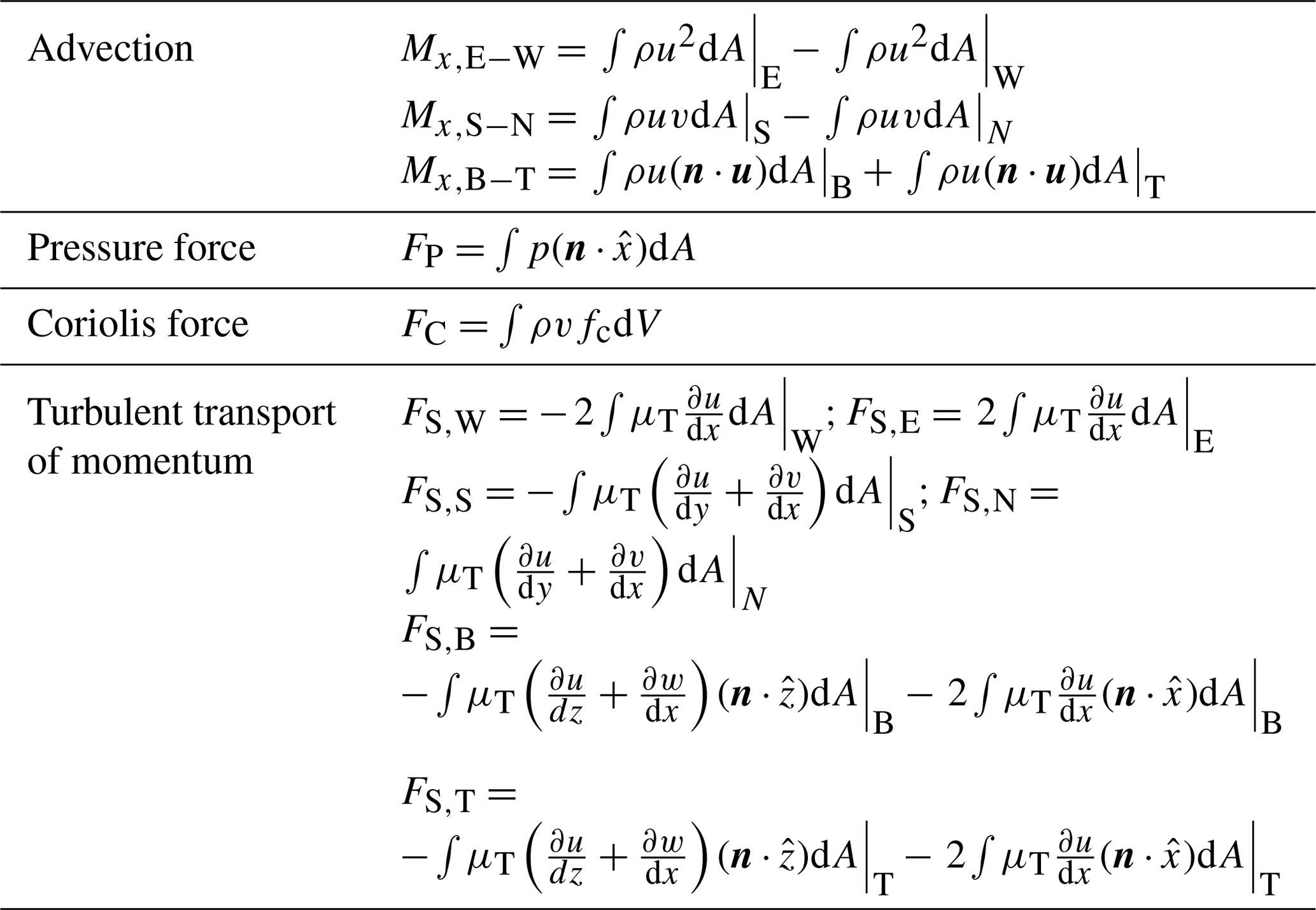
Table A1 shows how the terms in Eq. (A4) can be determined from the state variables of the RANS solutions. In these equations, u is the velocity vector, v is the y component of velocity, w is the z component of velocity, p is the pressure, μ_T is the turbulent viscosity, f_c is the Coriolis parameter, and n is the local surface normal pointing into the control volume.

The terms in Eq. (A4) were computed for each wind farm and freestream simulation. Figure A2 contains bar charts showing the values of these terms for the flat, hill windward, and hill leeward cases. The blue bars correspond to the wind farm simulations. The red bars correspond to the freestream simulations. All values are normalized by the M_x,W value for the corresponding simulation. The momentum accounting in Eq. (A4) should balance, but likely due to interpolation and discretization errors incurred during the post-processing of the RANS data, there is a small residual needed to balance the equation. The absolute value of the residual is less than 1 % of M_x,W in all cases (0.1 % for both flat simulations, 0.4 %–0.5 % for the hill windward simulations, and 0.5 %–0.6 % for the hill leeward simulations).

Note that in the following discussion on the contributors to $M_{x,\mathrm{E}-\mathrm{W}}$, we refer exclusively to the values in Fig. A2, which are normalized. When we write, for example, that the contribution of pressure is X% higher in the wind farm simulation compared with the freestream simulation for a given case, it means that F_P normalized by M_x,W in the wind farm simulation is X percentage points higher than F_P normalized by M_x,W in the freestream simulation.

The freestream solution for the flat case is nearly horizontally homogeneous (see Fig. A2a). Turbulent transport of momentum through the top and bottom surfaces are together in balance with a west-to-east pressure drop, such that the advection of momentum through the east surface is almost the same as that through the west surface. In the flat wind farm simulation, the advection of the x component of momentum is 3.7 % higher through the east surface than through the west surface. The primary contributor to this increase is the turbulent diffusion of momentum through the top surface (F_S,T). This normalized shear force, which is in the positive x direction, is much higher in the wind farm case than in the freestream case. The shear force on the bottom surface, which is in the negative x direction, is about the same in the wind farm case compared to the freestream case. The net effect is a positive contribution of turbulent diffusion to $M_{x,\mathrm{E}-\mathrm{W}}$ – enough to offset the negative contribution from the wind-farm-induced pressure field.

Wind-farm-induced pressure is generally higher just upstream of a wind farm than downstream of the wind farm; however, within a wind farm, material streamwise pressure increases induced by the wind farm itself can occur, which can affect wake recovery within the farm – as it does in the flat case. This effect is highlighted as a substantial negative influence on wake recovery between turbine rows in a simulated wind farm in Bastankhah et al. (2024).

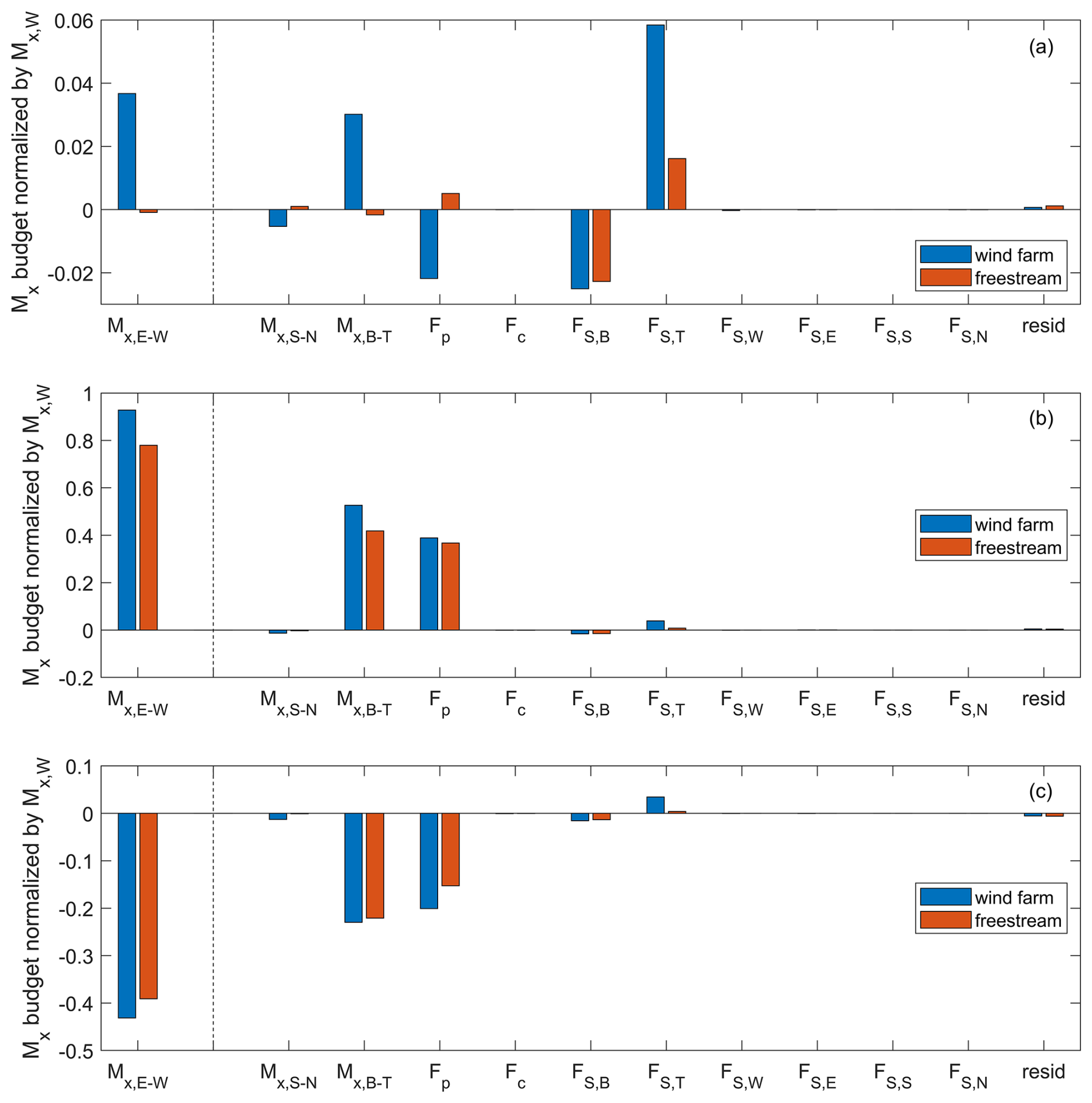
Figure A2 Budget for the x component of momentum from the CVA described in Fig. A1 for the flat case (a), the hill windward case (b), and the hill leeward case (c). The x axis labels correspond to the terms in Eq. (A4), normalized by M_x,W for each simulation.

The net advection of momentum through the top, bottom, and side surfaces in the flat case could be said to contribute to a positive $M_{x,\mathrm{E}-\mathrm{W}}$, although in this instance the contribution of vertical and lateral advection of momentum is closely linked with the turbulent diffusion of momentum. Turbulent diffusion in the flat case drives an increase in the advection of momentum through the east surface compared with the west surface. Mass conservation in turn requires a net inflow collectively from the other four surfaces (top, bottom, north, and south), which entails a net positive advection of x momentum collectively through these surfaces. One can then reasonably argue that the turbulent diffusion of momentum is the ultimate driver of wake recovery rather than the vertical advection of momentum. Of course, all the contributors to the momentum budget are coupled through the governing equations of the fluid flow. This fact can confound efforts to construct narratives of cause and effect. Nevertheless, we push forward with the control volume analysis with the goal of providing insight into the impact of terrain on wind farm flows and wake recovery – while bearing in mind that we will not be able to fully isolate the physical drivers behind this impact.

In the CVA of the wind farm simulation of the hill windward case (Fig. A2b), the advection of the x component of momentum through the east surface is nearly twice that of the momentum entering through the west surface. A significant pressure drop from west to east is a primary contributor to the increase in momentum. (The vertical advection of momentum is also a contributor; however, some of this contribution is very likely connected to the pressure drop, by continuity, as described just above.) The CVA of the freestream simulation also shows a large pressure drop from west to east as well as a large increase in the advection of the x component of momentum from west to east – though not as large as in the wind farm simulation. Turbulent transport of momentum through the top and bottom boundaries makes a net positive contribution to $M_{x,\mathrm{E}-\mathrm{W}}$ in the wind farm simulation (2.3 %), while the net contribution is slightly negative in the freestream case (−0.7 %). A comparison with the CVA for the flat case sheds light on why the wake recovery is greater between the first row and second row in the hill windward case. The improved wake recovery does not appear to be driven by turbulence, as the net contribution of turbulent diffusion to $M_{x,\mathrm{E}-\mathrm{W}}$ relative to freestream is smaller in the hill windward case (3.0 %) compared with the flat case (4.0 %). In contrast, the effect of terrain on pressure clearly increases wake recovery in the hill windward case compared with the flat case. In the hill windward case, the contribution of pressure to $M_{x,\mathrm{E}-\mathrm{W}}$ in the wind farm simulation is 2.2 % higher than in the freestream simulation; it is 2.7 % lower than freestream in the flat case. The deflection of the wake downward toward the ground in the hill windward case compared to the flat case also likely contributes to the increase in $M_{x,\mathrm{E}-\mathrm{W}}$, an effect that is included in $M_{x,\mathrm{B}-\mathrm{T}}$.

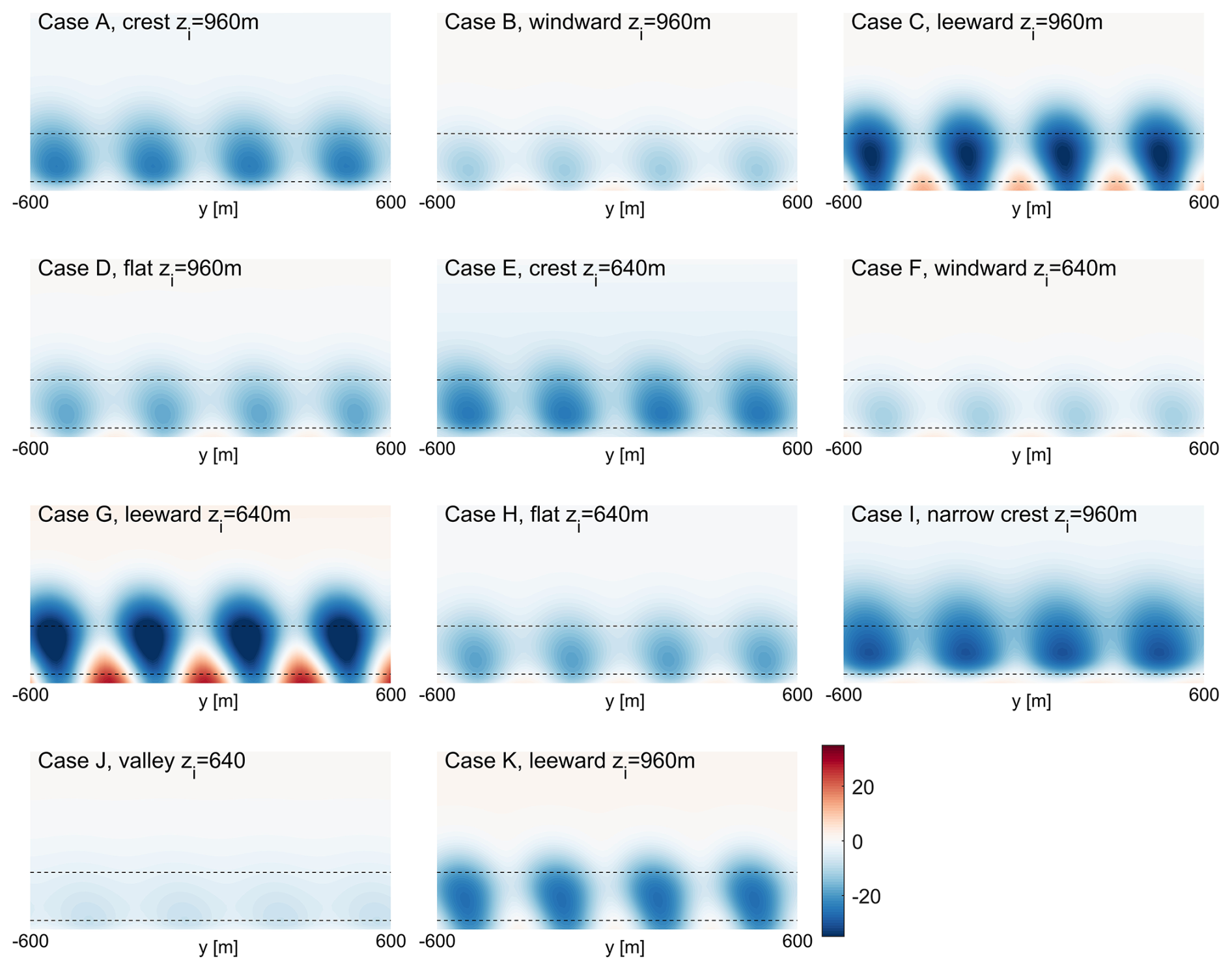
Figure A3 Percent change in wind speed relative to freestream on a vertical plane located 8 D downstream of the row of turbines for the 11 single-row cases for which top views of the percent change in wind speed are shown in Sect. 3.2. Dashed lines demark the rotor layer (heights of 35 and 195 m).

In the CVA of the wind farm simulation of the hill leeward case (Fig. A2c), the advection of the x component of momentum through the east surface is 43.1 % lower than through the west surface – which is 4.0 % lower than in the freestream simulation. There is no wake recovery between the west and east surfaces; the wake deficits instead become larger – the mean wind speed is 16.1 % lower than freestream at the west surface and 18.3 % lower than freestream at the east surface. The turbulent diffusion of momentum makes a net positive contribution to the $M_{x,\mathrm{E}-\mathrm{W}}$ budget relative to freestream (+2.8 %). This contribution is less than the net positive contribution of turbulent diffusion relative to freestream in the flat case (+4.0 %). Thus, differences in turbulent diffusion explain some of the difference in wake recovery between the flat and hill leeward cases; however, it cannot cause the negative wake recovery evident in the hill leeward case, where the wind speeds relative to freestream are lower at the east surface than the west. This is the result of a significant pressure rise from west to east. Relative to freestream conditions, the x component of the pressure force on the control volume in the wind farm simulation contributes −4.8 % to $M_{x,\mathrm{E}-\mathrm{W}}$. The deflection of the wake upwards in the hill leeward case relative to the flat case may also contribute to lowering $M_{x,\mathrm{E}-\mathrm{W}}$, although, as discussed in Sect. 3.1, the effect appears to be comparatively small.

Note that the turbulent transport of momentum contributes about the same amount to wake recovery in the hill windward case (3.0 %) as in the hill leeward case (2.8 %). The large difference in wake recovery between these two cases appears to have more to do with the substantial differences in the contributions of pressure.