Convolutional versus graph-based surrogate models for inter-farm wake prediction using multi-fidelity transfer learning

Accurate prediction of wind farm wake interactions is important for energy yield assessment, as offshore wind farms increasingly operate in close proximity to one another. This work presents a systematic comparison of two neural network surrogate models for inter-farm wake deficit prediction: a convolutional neural network (CNN)-based attention residual U-Net (ARU-Net) and a graph neural network (GNN)-based graph neural operator (GNO). Both architectures are trained using multi-fidelity transfer learning, pre-training with low-fidelity engineering model simulations, and then fine-tuning with high-fidelity Reynolds-averaged Navier–Stokes actuator wind farm (RANS-AWF) data. The models are evaluated on procedurally generated wind farm layouts spanning diverse farm sizes, turbine spacings, wind speeds, and ambient turbulence intensities. Both architectures achieve high prediction accuracy but exhibit complementary strengths: evaluated over the wake region (${\mathit{\delta }}_{\mathrm{w}}\ge {\mathrm{10}}^{-\mathrm{3}}$ m s⁻¹) and averaged across both evaluation grids, the GNO achieves a lower root mean squared error (RMSE) (0.024 vs. 0.028 m s⁻¹), while the ARU-Net attains a higher F₁ score (0.98 vs. 0.91), reflecting its superior wake boundary capture. Transfer learning substantially benefits the ARU-Net, while the GNO shows a smaller but measurable improvement, achieving its best performance with transfer learning.

1 Introduction

As global energy demand increases, and a number of areas suitable for offshore wind development become increasingly densely populated, the complexity of accurately modelling these environments has increased significantly. Multiple wind farms now operate in close proximity, creating complex flow interactions that extend far beyond single-farm boundaries. However, wake interactions between neighbouring farms remain poorly predicted by current engineering models, posing an important challenge for accurate energy yield assessment and wind farm layout optimisation (WFLO).

Wind farm wakes, defined as downstream regions of a wind farm with reduced wind speed and increased turbulence intensity (TI), have been observed to persist over remarkably long distances. Multiple independent measurement methodologies, including ground-based radar (Nygaard and Newcombe, 2018), scanning lidar systems (Schneemann et al., 2020; Cañadillas et al., 2022), synthetic aperture radar (SAR) satellite imagery (Hasager et al., 2015; Djath et al., 2018), and airborne measurement campaigns (Platis et al., 2018), have confirmed that wind farm wakes can extend far outside the wind farm boundaries and, under certain atmospheric conditions, beyond tens of kilometres, particularly for large wind farm clusters operating in stable atmospheric boundary layers. These observations challenge the fundamental assumptions of conventional engineering models, which are primarily developed and calibrated for intra-farm wake effects at distances of tens of rotor diameters.

Recent studies have further highlighted the importance of inter-farm wake interactions in wind farm clusters. Wang et al. (2022) showed that atmospheric stability and terrain can strongly affect wake persistence and downstream power losses for neighbouring onshore farms, while Wang et al. (2023) demonstrated that offshore cluster wakes may extend over very large distances as installed capacity increases. These findings further motivate the development of fast surrogate models for evaluating inter-farm wake effects across many layouts and inflow conditions.

Engineering wake models have served as the workhorses of wind farm design and energy yield assessment for the last few decades, offering computational efficiency and enabling the rapid evaluation of thousands of layout configurations during WFLO. Models such as the Park model by Jensen (1983), the Gaussian wake model of Bastankhah and Porté-Agel (2014), and the Turbulence Optimised Park model (TurbOPark) developed by Nygaard et al. (2020, 2022) are popular representative examples of analytical wake models.

The atmospheric conditions play an important role in wake persistence. Low turbulence, for instance, suppresses wake mixing, limiting downstream wake recovery, while high TI increases turbulent mixing, accelerating wake recovery. The interplay among atmospheric conditions, farm size, turbine spacing, and wake superposition creates a multidimensional parameter space that engineering models struggle to predict accurately.

Engineering wake models have fundamental limitations that become increasingly problematic at inter-farm scales. First, they assume steady-state, axisymmetric wake structures, neglecting the inherent unsteadiness and three-dimensional complexity of turbulent wakes. Second, they rely on algebraic superposition methods, typically linear or squared-sum approaches, to combine multiple single-turbine wakes. While computationally efficient, superposition does not capture the non-linear wake interactions that occur when multiple wakes merge and interact with the atmospheric boundary layer. Third, these models neglect large-scale atmospheric effects, including Coriolis forces, atmospheric stability, and mesoscale flow phenomena, that become relevant at distances of tens of kilometres. Even when calibrated to specific sites or conditions, engineering models lack the physical fidelity to generalise across the diverse operating conditions met in practice. When designing a wind farm, consideration must be given to neighbouring wind farms, as wake losses from neighbouring projects may affect profitability. Multiple neighbours may be present simultaneously, and at the time of freezing the design, their layouts might not yet be finalised and subsequently change. Accounting for these inter-farm effects is therefore challenging due to the inherent uncertainty surrounding the configuration of neighbouring projects, and a fast, accurate model is needed to efficiently evaluate many candidate designs.

Data-driven surrogate models have gained popularity as they bridge the accuracy–efficiency gap in wind farm flow modelling. By learning mappings from input parameters, like wind farm layout and inflow conditions, to output flow fields directly from simulation data, these models can achieve prediction speeds comparable to engineering models while capturing more of the complex physics of the training data. However, the accuracy of data-driven surrogates is fundamentally constrained by the fidelity of the training data. Therefore, a model trained exclusively on engineering model outputs cannot exceed the engineering accuracy of the model, regardless of how sophisticated the fully data-driven neural network architecture is.

Reynolds-averaged Navier–Stokes (RANS) or large-eddy simulations (LES) are more physically accurate, but computationally much more expensive than low-fidelity engineering models. On the other hand, idealised RANS and LES cannot account for the large and mesoscale scales of the atmospheric flow. Therefore, a common method for simulating inter-farm wake effects is to use wind farm parameterisations implemented in numerical weather prediction models. Although such models realistically simulate atmospheric processes across large spatial domains, their spatial resolutions are too coarse to account for individual wind turbine wakes. Therefore, the accuracy of these parameterisations is currently a matter of debate (Peña et al., 2022; García-Santiago et al., 2024). This observation motivates multi-fidelity transfer learning approaches that utilise both the abundant low-fidelity data and sparse high-fidelity data. The strategy involves pre-training neural network models on large datasets generated by computationally inexpensive engineering models, thereby establishing robust representations of fundamental wake physics and layout-to-flow mappings. These pre-trained models can then be fine-tuned on smaller datasets of high-fidelity simulations, enabling them to learn corrections to engineering model predictions while avoiding overfitting to limited data.

Within this multi-fidelity surrogate modelling framework, convolutional neural networks (CNNs) and graph neural networks (GNNs) represent two principal architectural paradigms for learning layout-to-flow mappings from simulation data. In this work, two principal families of neural network architectures have been applied to wind farm flow prediction: CNNs and GNNs. These architectures differ in how they interpret spatial information and how they handle wind farm geometry. CNNs operate with flow fields on a regular grid, treating the spatial domain as a regular, image-like structure, while the GNNs operate on the more adaptive structure of a graph.

Both neural network architectures can be trained to predict the flow field around different layouts, but the two methods use different methods of encoding turbine placement. In most CNN-based approaches, it is necessary to rasterise locations onto a fixed spatial domain, whereas turbine positions can be placed exactly at graph nodes, as the graph is adaptive. However, this depends on how the graph is constructed. Graphs can broadly be divided into two categories: extrinsic graphs, where the nodes and edges form a spatial mesh, and intrinsic graphs, where the nodes correspond directly to the physical entities of interest, in the context of wind farms typically the turbines themselves.

Multiple previous studies have applied CNN-based architectures to aerodynamic and wind flow prediction tasks. Thuerey et al. (2019) demonstrated that a U-Net encoder–decoder architecture could serve as an effective RANS surrogate for predicting velocity and pressure fields around airfoils, establishing the viability of convolutional auto-encoders (CAEs) for learning complex flow patterns from simulation data. Hasanpoor et al. (2025) developed a physics-informed deep convolutional hierarchical encoder–decoder neural network for predicting flow fields within wind farms, incorporating physical constraints to improve generalisation. Li et al. (2022a) proposed their Super-Fidelity Network (SFNet), which utilises a CNN-based model for super-resolution-type task mapping between low-fidelity engineering models and high-fidelity LES data. Anagnostopoulos et al. (2023) employed CNN-based wake models within a multi-fidelity deep transfer learning framework to accelerate wind farm yaw and layout optimisation, demonstrating that features learned from low-fidelity wake simulations could be transferred to improve predictions at higher fidelity levels.

Similarly, GNNs have previously been explored in the literature: Park and Park (2019) trained a physics-induced graph neural network (PGNN) for power estimation in wind farms. Bleeg (2020) trained a GNN as an RANS surrogate to predict turbine wind speeds. Ødegaard Bentsen et al. (2022) employed a graph attention network (GAT) to predict individual turbine power production. Duthé et al. (2023, 2024) created a GNN using intrinsic graphs for load estimation of the turbines. Li et al. (2024) demonstrated a graph transformer for power estimation with yaw angle variations. Daenens et al. (2025) implemented a spatio-temporal GNN capable of predicting the power of individual turbines by processing node input signals with a long short-term memory (LSTM) model rather than a conventional multi-layer perceptron (MLP). Wang et al. (2026) demonstrated a graph transformer with a hybrid approach, which they termed a knowledge-fusion graph transformer (KFGT), capable of predicting the turbine-level flow and loads. Hou et al. (2026) demonstrated a two-stage GNN with a novel approach to turbine connectivity using a hybrid approach.

1.1 Our contribution

In our own previous work, we have explored both a CNN-based architecture; the attention residual U-Net (ARU-Net) (Rasmussen et al., 2026); and a GNN-based approach, the graph neural operator (Schøler et al., 2026). In Rasmussen et al. (2026), a two-stage transfer learning strategy was applied, pre-trained on the Gaussian engineering model by Zong and Porté-Agel (2020) and fine-tuned on Reynolds-averaged Navier–Stokes actuator wind farm (RANS-AWF) (van der Laan et al., 2023) data. The present work builds on this foundation by extending the ARU-Net architecture with feature-wise linear modulation (FiLM) conditioning, using a variant of parameter-efficient fine-tuning (PEFT), namely low-rank adaptation (LoRA), and by directly comparing its performance with that of a graph-based alternative.

In Schøler et al. (2026), we demonstrated a methodology to predict a flow field using a graph neural operator (GNO), an intrinsic graph approach where each node represents a physical wind turbine. However, to predict at a random location, we introduced probe nodes in addition to the intrinsic wind farm nodes. This probe node formulation shares some similarities with the extrinsic approach, as they can be placed at arbitrary spatial locations rather than at physical entities.

In this work, we present a systematic comparison of the ARU-Net and the GNO for multi-fidelity transfer learning in inter-farm wake modelling. Both architectures are pre-trained on a large dataset generated using the TurbOPark engineering model (Nygaard et al., 2022) implemented in PyWake (Pedersen et al., 2023), then fine-tuned on RANS-AWF data using PyWakeEllipSys (DTU Wind and Energy Systems, 2026) simulations with LoRA-based PEFT. This common multi-fidelity workflow enables a direct comparison of raster-based and graph-based surrogate modelling approaches under the same low- and high-fidelity training stages. We evaluate wind speed prediction accuracy across diverse wind farm layouts and inflow conditions; analyse spatial performance, including wind speed error distributions; and assess sensitivity to farm size and atmospheric inflow conditions.

The remainder of this paper is organised as follows: Sect. 2 describes the methodology, including wind farm flow modelling approaches, procedural data generation, neural network architectures, and training procedures. Section 3 presents the results and discussion for both models, covering qualitative and quantitative analyses alongside an assessment of the implications for practical wind farm modelling applications. Section 4 concludes with a summary of the results, an overview of the qualitative differences between the models, and directions for future research.

2 Methodology

In this section, the simulation tools and the neural network architectures are described. However, first, a broader comparison of CNNs and GNNs is presented to clarify their similarities and differences.

2.1 On the connection between CNNs and GNNs

In fields such as computer vision and medical science, CNNs have shown usefulness across many diverse applications. Most users of machine learning (ML) in wind energy have worked with CNNs. Although GNNs are gaining wider adoption within the wind energy community, they remain under-investigated. In this section, an analogy between CNNs and GNNs is presented.

A grid can be viewed as a specific type of graph where the connections of the nodes are fixed on a regular lattice; see e.g. Bronstein et al. (2021, Sects. 3.4 and 4.2) for a thorough introduction to the concepts and Sanchez-Lengeling et al. (2021) for an interactive introduction. This abstraction carries important implications for the relationship between CNNs and GNNs. Graphs used in scientific machine learning (SciML) can be broadly placed on a spectrum between two poles. At one end lie extrinsic (discretised) graphs: the nodes and edges form a mesh that approximates an underlying continuous field. The graph is a computational artefact. One could remesh at a different resolution or with a different triangulation and still represent the same physical domain. At the other end lie intrinsic (native) graphs, where the nodes correspond to the actual entities of interest, and the topology is physically meaningful. A graph whose nodes are wind turbines and whose edges encode relative positional information between them is an example: the topology directly reflects the physical layout of the farm, and there is no finer-resolution version of that layout to recover. CNNs operate exclusively on discretised, regular grids of pixel positions, e.g. on an image or, in the present context, cell centres in the flow field grid.

At a high level, CNNs and GNNs can both be viewed as local aggregation methods. A CNN applies a learned kernel over neighbouring cells on a regular grid, while a GNN aggregates information through message passing over graph edges. This analogy is illustrated in Fig. 1, with a more detailed mathematical discussion provided in Appendix A.

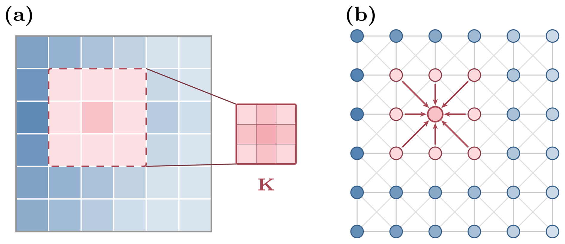
Figure 1 Comparison of local aggregation operations: (a) convolution applies a learned kernel K over a regular grid, aggregating values from a fixed spatial neighbourhood; (b) message passing aggregates features from neighbouring nodes on a graph with a fixed grid domain.

On a regular pixel grid, a single convolutional layer can only aggregate information from a small spatial neighbourhood defined by the kernel size. For wind farm wake modelling, where upstream turbines are far away from downstream conditions, this local view is insufficient. Deeper architectures address this limitation: in a plain CNN, stacking n_depth convolutional layers linearly increases the active domain with depth, while convolutional encoder–decoder architectures, such as the U-Net, go further by compressing the spatial domain using downsampling, allowing deeper layers to see increasingly larger portions of the domain. The methodology is depicted in Fig. 2a.

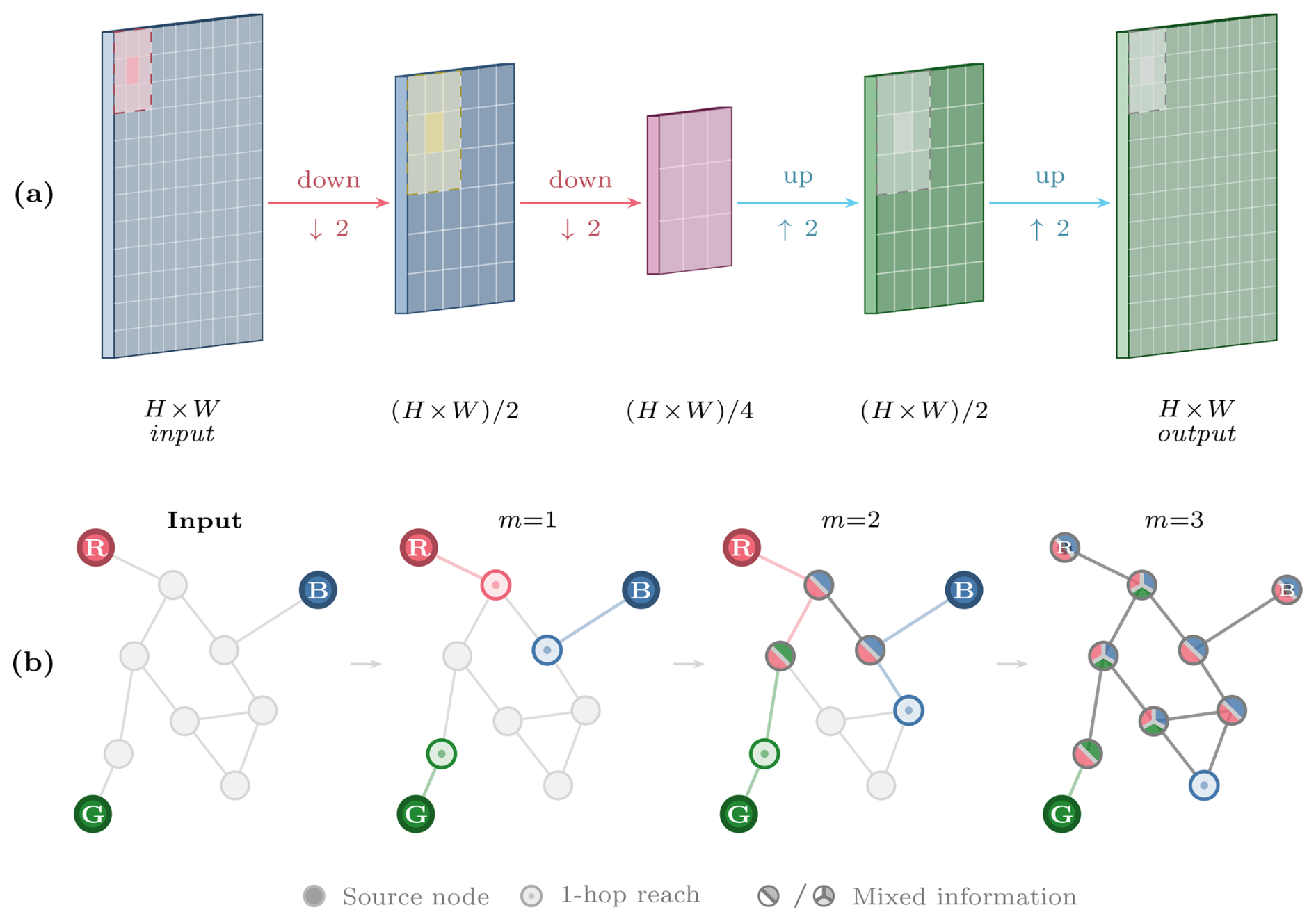
Figure 2 Depth as a mechanism for multi-scale information aggregation. (a) A CNN operating on an input domain of size H×W growing its effective domain through successive downsampling layers: a local 3×3 kernel covers the full spatial domain after two downsampling stages. (b) A GNN spreads information progressively via message-passing steps (m).

Unlike CNNs, which are inherently defined on regular grids, GNNs operate on arbitrary graph structures, where the choice of intrinsic or extrinsic topology is specified as part of the model architecture prior to training. When the graph is a discretised mesh, similar to grids regularly used for computational fluid dynamics (CFD), as in the MeshGraphNets framework of Pfaff et al. (2021), the message-passing mirrors the spatial discretisation of the computational domain. Stacking message-passing layers then serves a purpose similar to stacking convolutional layers: each additional step propagates information one step further across the mesh, gradually extending the spatial reach of the model. Two examples relevant to wind energy flow modelling include Li et al. (2022b), who created a single-turbine RANS-based GNN wake surrogate model using a discredited mesh, and Duthé et al. (2025), who demonstrated a mesh-type GNN that is used to create realistic realisations of the flow around an airfoil given knowledge of the airfoil boundary.

In contrast, when the graph is intrinsic, as in this work, where each node represents a wind turbine, and the edges encode positional relations, a single message-passing step already exchanges information directly between the turbines. Stacking additional layers, therefore, takes on a different role. Rather than extending the spatial reach in a grid, it enables the model to consider turbine interactions outside the direct neighbourhood of each local turbine, thereby connecting the turbines into a farm. A visualisation of GNN message passing in connection with depth is illustrated in Fig. 2b, where three source nodes are not directly connected, but information is exchanged between them after successive message-passing steps (m).

2.2 Wind farm engineering model

To generate the low-fidelity dataset, we use the open-source tool PyWake (Pedersen et al., 2023). PyWake is a modular implementation of various engineering modelling tools, including wake deficit models, added TI models, blockage, wake deflection, and mirroring. We employ the Turbulence Optimised Park model (TurbOPark) with the Gaussian wake profile developed by Nygaard et al. (2022). TurbOPark was selected because it was calibrated for far-wake and cluster-wake applications and showed the closest agreement with RANS-AWF among the engineering models we tested.

The model incorporates the added TI formulation of Frandsen (2007) directly into the wake expansion, eliminating the need for a standalone TI model. For combining multiple wakes, it uses squared-sum superposition, motivated by energy-deficit arguments (Porté-Agel et al., 2020), a ground-mirroring model to implement the surface boundary condition, and a Gaussian overlap model for rotor averaging. The wake deficit model is given by

$$\begin{array}{ll}\text{(1a)}& {\displaystyle \frac{\mathrm{\Delta }u}{U_{\mathrm{\infty }}}}& {\displaystyle }=C\exp \left(-{\displaystyle \frac{r^{\mathrm{2}}}{\mathrm{2}{\mathit{\sigma }}_{\mathrm{w}}^{\mathrm{2}}}}\right),C=\mathrm{1}-\sqrt{\mathrm{1}-{\displaystyle \frac{C_{\mathrm{T}}}{\mathrm{8}({\mathit{\sigma }}_w/D{)}^{\mathrm{2}}}}},{\displaystyle \frac{{\mathit{\sigma }}_w}{D}}& {\displaystyle }=\mathit{\epsilon }+{\displaystyle \frac{\mathrm{0.04}{I}_{\mathrm{0}}}{\mathit{\beta }}}\left(\sqrt{(\mathit{\alpha }+\mathit{\beta }\mathit{\xi }{)}^{\mathrm{2}}+\mathrm{1}}-\sqrt{\mathrm{1}+{\mathit{\alpha }}^{\mathrm{2}}}\right.\\ \text{(1b)}& {\displaystyle }& {\displaystyle }\left.-\ln \left[{\displaystyle \frac{(\sqrt{(\mathit{\alpha }+\mathit{\beta }\mathit{\xi }{)}^{\mathrm{2}}+\mathrm{1}}+\mathrm{1})\mathit{\alpha }}{(\sqrt{\mathrm{1}+{\mathit{\alpha }}^{\mathrm{2}}}+\mathrm{1})(\mathit{\alpha }+\mathit{\beta }\mathit{\xi })}}\right]\right),{\displaystyle }\mathit{\alpha }& {\displaystyle }=\mathrm{1.5}{I}_{\mathrm{0}},\mathit{\beta }={\displaystyle \frac{\mathrm{0.8}{I}_{\mathrm{0}}}{\sqrt{C_{\mathrm{T}}}}},\\ \text{(1c)}& {\displaystyle }& {\displaystyle }\mathit{\epsilon }=\mathrm{0.25}\sqrt{{\displaystyle \frac{\mathrm{1}+\sqrt{\mathrm{1}-{\widehat{C}}_{\mathrm{T}}}}{\mathrm{2}\sqrt{\mathrm{1}-{\widehat{C}}_{\mathrm{T}}}}}},{\widehat{C}}_{\mathrm{T}}=min(C_{\mathrm{T}},\mathrm{0.96}),\end{array}$$

where Δu is the velocity deficit, U_∞ the free-stream velocity, r the radial distance from the wake centreline, σ_w the characteristic wake width,  D the rotor diameter, $\mathit{\xi }=x/D$ the dimensionless downstream distance, C_T the thrust coefficient, and I₀ the ambient TI. The coefficient C represents the centreline maximum velocity deficit. The parameters α and β, which govern the turbulence-dependent wake expansion rate, are adopted from Frandsen (2007); the coefficient 0.04 was calibrated by Nygaard et al. (2022) against operational data from 19 offshore wind farms. The initial wake width ε follows the formulation of Bastankhah and Porté-Agel (2014).

Despite its calibration including far-wake physics, TurbOPark shares limitations common to engineering wake models: it assumes steady, axisymmetric wakes; neglects large-scale atmospheric effects; and relies on algebraic superposition, which does not fully capture wake interactions.

2.3 Reynolds-averaged Navier–Stokes with actuator wind farm (RANS-AWF)

RANS-AWF simulations offer higher physical fidelity than engineering models by resolving the mean flow field around wind farms, including pressure gradients and wake boundary layer interactions, while representing turbines through distributed momentum sink terms.

The high-fidelity dataset is produced with EllipSys3D (Michelsen, 1992; Sørensen, 1995), coupled to the AWF model of van der Laan et al. (2023). In this formulation, the RANS equations are closed by the k-ε-f_P turbulence closure (van der Laan et al., 2015), and each wind farm enters the momentum equations as a distributed drag force analogous to a forest canopy. A surrogate trained on higher-resolution actuator-disc simulations (van der Laan et al., 2026a) provides the wind farm thrust coefficient, enabling accurate long-distance wake prediction at moderate computational cost. A single RANS-AWF simulation takes only a few minutes using multiple nodes on a high-performance computing (HPC) cluster (Technical University of Denmark, 2019).

A neutral atmospheric surface layer is employed by prescribing a logarithmic streamwise velocity profile, a constant turbulence kinetic energy (TKE), and a profile of the TKE dissipation at both the inlet and top boundaries. Inflow TI is governed by the surface roughness length z₀, which we relate to a prescribed streamwise I₀ via

$$\begin{array}{}\text{(2)}& z_{\mathrm{0}}=z_H\exp \left(-{\displaystyle \frac{\mathrm{1}}{I_{\mathrm{0}}}}\right).\end{array}$$

Because the k-ε-f_P turbulence closure is formulated in terms of a turbulence kinetic energy (TKE)-based turbulence intensity $I_{\mathrm{TKE}}=\sqrt{\mathrm{2}k/\mathrm{3}}/U_{\mathrm{\infty }}$ rather than the streamwise component, a conversion is needed to map to the ambient TI, I₀. In the atmospheric surface layer, turbulence is anisotropic, with streamwise fluctuations exceeding those in the vertical and lateral directions (van der Laan et al., 2015). We therefore adopt I_TKE≈0.8 I₀. The sampled range for the RANS-AWF dataset is $I_{\mathrm{0}}\in [\mathrm{0.03},\mathrm{0.25}]$, corresponding to roughness lengths $z_{\mathrm{0}}\in [\sim {\mathrm{10}}^{-\mathrm{12}},\sim \mathrm{2}]$ m.

The numerical domain represents a Cartesian grid with dimensions $\mathrm{1522}D\times \mathrm{1266}D\times \mathrm{25}D$ in the streamwise (x) lateral (y), and vertical (z) directions, respectively. The wind farm is placed at the horizontal origin of the domain, $\mathit{\{}x,y\mathit{\}}=\mathit{\{}\mathrm{0},\mathrm{0}\mathit{\}}$, which is located 569 D from the inlet boundary and 633 D from the lateral boundaries. A region around the wind farm, with dimensions of $-\mathrm{69}<x/D<\mathrm{453}$ and $-\mathrm{133}<y/D<\mathrm{133}$, is defined, at which a cell spacing of 2 D is applied, based on a grid refinement study (van der Laan et al., 2023). The horizontal cell sizes are stretched towards the lateral, inlet, and outlet boundaries with a maximum growth ratio of 1.2, covering a distance of 500 D. The vertical cell distribution consists of a first cell height of $D/\mathrm{200}$ that is initially stretched towards a cell height of $D/\mathrm{6}$ at $z/D=\mathrm{3}$ and then further stretched towards the top boundary. In total, 3.9 million cells are used, distributed as $\mathrm{320}\times \mathrm{192}\times \mathrm{64}$ in the horizontal, lateral, and vertical directions, respectively. The logarithmic inflow is prescribed at the inlet and top boundary, resulting in a lid-driven flow setup. A fully developed flow is assumed at the outlet, at which all gradients normal to the outlet plane are assumed to be zero. The bottom boundary is a rough wall boundary (Sørensen et al., 2007), and the lateral boundaries are periodic. The hub height plane at 119 m is extracted from each simulation and interpolated onto a 256×128 Cartesian grid consistent with the low-fidelity domain, with 64 vertical levels. The resulting dataset comprises 1000 samples from 250 distinct layouts, each evaluated at four uniformly sampled inflow conditions, and is partitioned into 700 for training, 100 for validation, and 200 for test cases.

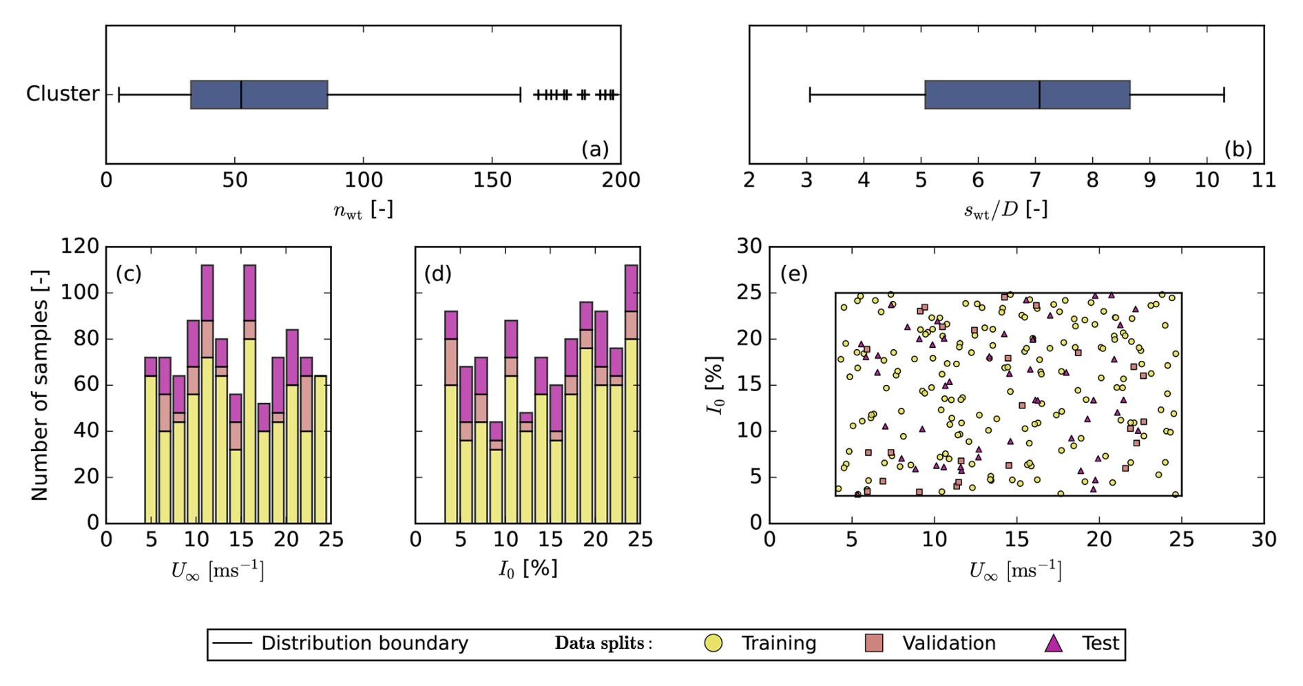
Figure 3 Procedurally generated data for the RANS-AWF dataset, (a–b) statistics of generated layouts, (c) U distribution, (d) ambient TI distribution, and (e) generated U and I₀ samples with boundary.

2.4 Procedural data generation

To ensure the models are trained on a broad range of layouts and inflow conditions, a procedural data generation strategy is adopted for the engineering model dataset. The method is adopted from Schøler et al. (2026), but with two improvements: (i) layout-specific number of wind turbines (n_wt) and turbine separation factors (s_wt) defining the smallest allowed distance between turbines and (ii) capping I₀ at 80 % to limit the number of extreme cases. An overview of the method as applied when generating the low-fidelity dataset is shown in Fig. 4.

The RANS-AWF dataset is repurposed from Rasmussen et al. (2026) and therefore does not utilise the same sampling strategy. In Rasmussen et al. (2026), wind farm layouts were generated by placing turbines within random polygons using Poisson disc sampling with minimum spacing constraints between 3 D and 10 D, similar to the cluster generation mode in PLayGen. Random turbine removal, with a probability of 0 %–50 %, was applied to increase layout diversity. As the RANS-AWF dataset used in this work only contains the equivalent of the cluster layout type, the resulting models are therefore not expected to generalise as well to the remaining layout types. Future datasets should incorporate a broader range of layouts to address this limitation in subsequent works.

Inflow conditions were sampled uniformly with $U_{\mathrm{\infty }}\in [\mathrm{4},\mathrm{25}]$ m s⁻¹ and $I_{\mathrm{0}}\in [\mathrm{0.03},\mathrm{0.25}]$, treating wind speed and turbulence intensity as independent variables. This contrasts with the engineering model dataset, in which U and σ_u are coupled through the correlated International Electrotechnical Commission (IEC)-based sampling framework. The RANS-AWF sampling domain can largely be considered a subset of the engineering model inflow range. However, because the IEC-based upper bound on σ_u (Eq. 3b) decays with increasing wind speed, the correlated Sobol sequence does not populate the corner of the (U_∞,I₀) space, where both quantities are simultaneously high. A small number of uniformly sampled RANS-AWF points occupy this region and therefore fall outside the engineering model's inflow coverage.

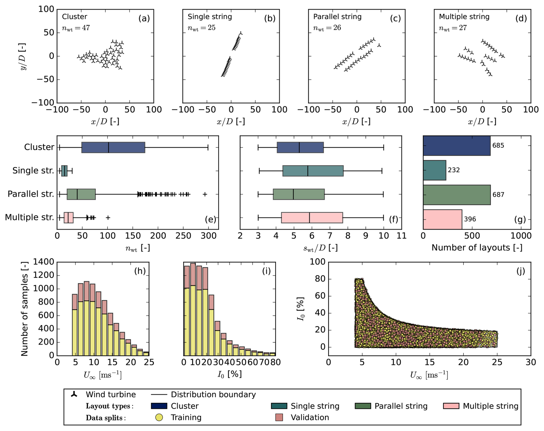
Figure 4 Procedurally generated data for the engineering model dataset, (a–d) examples of wind farm layout types in PLayGen, (e–g) statistics of generated layouts, (h) U distribution, (i) ambient TI distribution, and (j) generated U and I₀ samples with boundary.

Wind farm layout generation

To generate the wind farm layouts, the Plant Layout Generator (PLayGen) by Harrison-Atlas et al. (2024) is used. PLayGen generates four types of layouts: cluster, which consists of irregularly distributed turbines across the domain; single-string layouts, which arrange turbines along a single curved string with periodic gaps; parallel-string layouts, which feature multiple strings sharing an orientation, similar to conventional offshore wind farms; and multiple-string layouts, which comprise several strings with independent orientations, resulting in configurations with strings at multiple angles. Examples are shown in Fig. 4a–d.

Inflow sampling

For each layout, we consider four different combinations of inflow conditions, meaning four combinations of the free-stream velocity U and ambient turbulence intensity I₀. These parameters are coupled in the atmospheric boundary layer, so we employ the correlated sampling framework of Dimitrov et al. (2018) to generate physically realistic combinations. Following updates to IEC 61400-1  (2019), we adopt the A⁺ turbulence class with reference intensity $I_{\mathrm{ref},{\mathrm{A}}^{+}}=\mathrm{0.18}$. An upper bound of $I_{\mathrm{0},\max }=\mathrm{0.8}$ was set to avoid overly extreme flow cases.

The operational velocity range is set by the DTU 10 MW reference turbine (Bak et al., 2013), which has a rotor diameter D=178.3 m, cut-in wind speed $U_{\mathrm{c},\mathrm{in}}=\mathrm{4}$ m s⁻¹, rated wind speed U_rated=11.4 m s⁻¹, and cut-out wind speed $U_{\mathrm{c},\mathrm{out}}=\mathrm{25}$ m s⁻¹. Bounds on the velocity standard deviation σ_u follow Dimitrov et al. (2018, Tab. 1):

$$\begin{array}{ll}\text{(3a)}& {\displaystyle }\mathrm{4}\mathrm{m}{\mathrm{s}}^{-\mathrm{1}}& {\displaystyle }\le U_{\mathrm{\infty }}\le \mathrm{25}\mathrm{m}{\mathrm{s}}^{-\mathrm{1}},{\displaystyle }\mathrm{0.0025}{U}_{\mathrm{\infty }}& {\displaystyle }\le {\mathit{\sigma }}_{\mathrm{u}}\le I_{\mathrm{ref},{\mathrm{A}}^{+}}\left(\mathrm{6.8}+{\displaystyle \frac{\mathrm{3}}{\mathrm{4}}}{U}_{\mathrm{\infty }}+\mathrm{3}{\left({\displaystyle \frac{\mathrm{10}}{U_{\mathrm{\infty }}}}\right)}^{\mathrm{2}}\right)\\ \text{(3b)}& {\displaystyle }& {\displaystyle }\left[\mathrm{m}{\mathrm{s}}^{-\mathrm{1}}\right].\end{array}$$

We populate the inflow space using quasi-Monte Carlo sampling with the improved Sobol sequence of Joe and Kuo (2008). Although Dimitrov et al. (2018) used the Halton sequence, we found that the Sobol sequence achieves better coverage of the distribution tails (Schøler et al., 2026). The velocity samples are mapped through a Rayleigh distribution following IEC 61400-1  (2019) and scaled to the bounds in Eq. (3a). The turbulence samples are transformed via Eq. (3b) to obtain σ_u, which is then converted to ambient TI through $I_{\mathrm{0}}={\mathit{\sigma }}_{\mathrm{u}}/U_{\mathrm{\infty }}$. The resulting TI distribution is shown in Fig. 4j.

2.4.1 Dataset configuration

Table 1 summarises the dataset configuration for both fidelity levels. Both architectures are trained on the same layouts and inflow conditions to permit a fair comparison. However, the data representations differ. The ARU-Net operates on gridded flow fields of shape $\mathrm{256}\times \mathrm{128}\times \mathrm{1}$, whereas the GNO represents each layout as a graph whose turbine nodes carry positional and inflow features and whose probe nodes are placed at evaluation locations. The two models are evaluated on two distinct grids, the CNN grid (256×128) and the GNN grid (257×129), to assess the sensitivity of each model to the grid changes (Sect. 3.4).

(Dimitrov et al., 2018)

Table 1 Dataset configuration for low-fidelity and high-fidelity simulations.

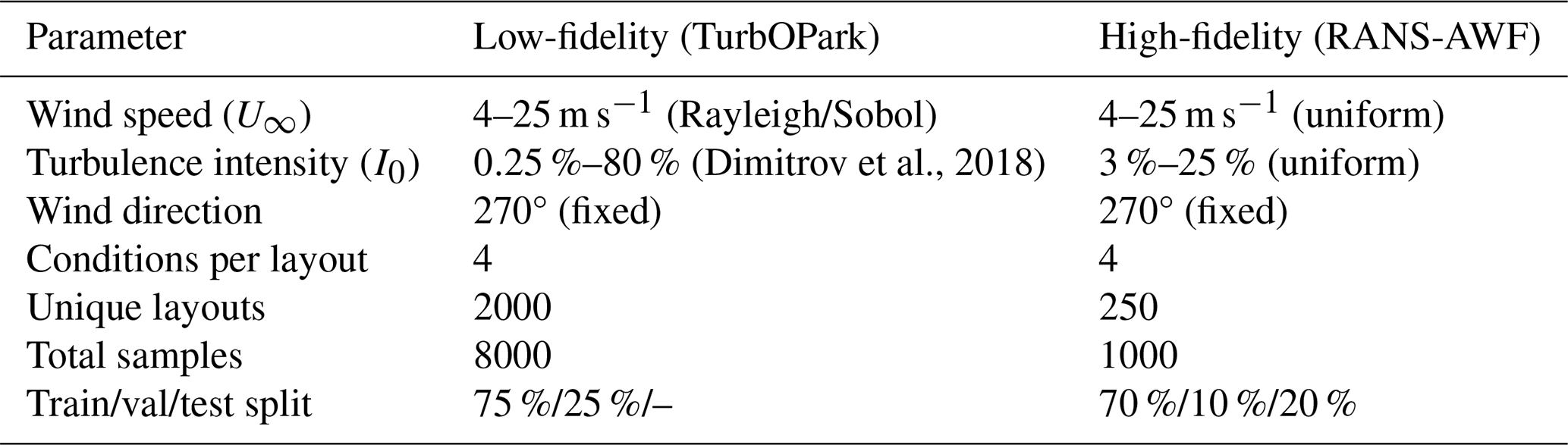
The low-fidelity dataset comprises 8000 TurbOPark simulations generated from 2000 unique layouts, each evaluated at four inflow conditions sampled using the correlated IEC-based framework of Dimitrov et al. (2018), as described in Sect. 2.4.2. The high-fidelity dataset consists of 1000 RANS-AWF simulations repurposed from Rasmussen et al. (2026), where the layouts were generated as cluster-like farm configurations using random farm polygons and Poisson disc turbine placement. It comprises 250 unique layouts, each evaluated at four uniformly sampled inflow conditions with $U_{\mathrm{\infty }}\in [\mathrm{4},\mathrm{25}]$ m s⁻¹ and $I_{\mathrm{0}}\in [\mathrm{0.03},\mathrm{0.25}]$, and is partitioned into 700 training, 100 validation, and 200 test samples. An overview of the RANS-AWF dataset is presented in Fig. 3. Consequently, the present fine-tuning results mainly assess generalisation within cluster-like farm layouts rather than across all PLayGen layout classes. In both datasets, layouts are assigned to a single data split before inflow sampling, ensuring that no identical layout appears in both the training and evaluation sets. A key difference between the two datasets is the distribution of inflows. The low-fidelity data span a substantially wider turbulence intensity range (I₀ up to 80 %; Fig. 4i–j) using the correlated sampling of Dimitrov et al. (2018), whereas the RANS-AWF data are restricted to $I_{\mathrm{0}}\in [\mathrm{0.03},\mathrm{0.25}]$ (see Fig. 3e). Figure 5 shows the domain in which the data are generated.

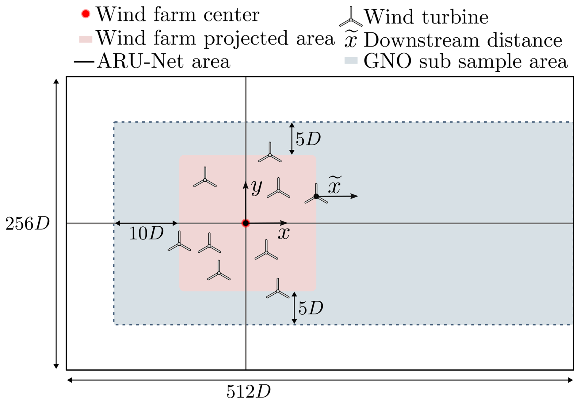
Figure 5 Modelling domain shared by the U-Net and GNO, indicating the spatial subset of probe locations used when training the GNO.

For data generation, the same fixed-resolution domain for all layouts is required by the CNN-based approach. For the GNO, no fixed grid is necessary. Owing to its grid invariance, only a spatial subset of the domain is queried during training to improve computational efficiency. This concept is shown in Fig. 5.

2.5 Attention residual U-Net (ARU-Net)

The attention residual U-Net (ARU-Net) is a convolutional surrogate model that predicts wind farm wake fields from turbine layout rasters and inflow specifications. Its architecture follows the encoder–decoder paradigm established by U-Net (Ronneberger et al., 2015), with several enhancements to improve feature extraction and gradient flow. The encoder extracts hierarchical spatial features through successive downsampling stages. The bottleneck integrates inflow conditions, and the decoder reconstructs the flow field at the original resolution via skip connections that preserve fine-grained spatial information. A similar architecture was previously used in a multi-fidelity transfer learning context in Rasmussen et al. (2026). The remainder of this section describes the configuration used in the present work.

The encoder comprises six resolution levels connected by five downsampling stages, with channel counts increasing at each stage and a fixed maximum channel count. Each encoder block contains two 3×3 convolutional layers with residual connections,

$$\begin{array}{}\text{(4)}& {\mathit{h}}^{\left(l\right)}={\mathit{\psi }}_{\mathrm{m}}\left(\mathcal{F}({\mathit{h}}^{(l-\mathrm{1})};{\mathit{\theta }}^{\left(l\right)})+\mathcal{P}\left({\mathit{h}}^{(l-\mathrm{1})}\right)\right),\end{array}$$

where ℱ denotes the stacked convolution–normalisation transformation with learnable parameters θ^(l), 𝒫 is a 1×1 projection that matches channel dimensions when necessary, and ψ_m=Mish (Misra, 2020) is the activation function. Group normalisation is applied after each convolution. Downsampling employs a learned Gaussian blur filter to avoid spatial aliasing artefacts, while the decoder uses transposed convolutions for upsampling. Squeeze-and-excitation (SE) blocks (Hu et al., 2018) provide channel-wise feature recalibration within each encoder and decoder block, as seen in Eq. (5):

$$\begin{array}{}\text{(5a)}& {\displaystyle }\mathit{z}& {\displaystyle }={\displaystyle \frac{\mathrm{1}}{HW}}\sum _{i,j}{\mathit{h}}_{i,j},\text{(5b)}& {\displaystyle }\mathit{s}& {\displaystyle }={\mathit{\psi }}_{\mathrm{s}}\left({\mathbf{W}}_{\mathrm{2}}{\mathit{\psi }}_{\mathrm{r}}\left({\mathbf{W}}_{\mathrm{1}}\mathit{z}\right)\right),\text{(5c)}& {\displaystyle }\stackrel{\mathrm{̃}}{\mathit{h}}& {\displaystyle }=\mathit{s}\odot \mathit{h},\end{array}$$

where z is the spatially pooled feature vector, W₁ and W₂ are learnable weights with a reduction factor of 16, ψ_r is the rectified linear unit (ReLU) activation function (Agarap, 2019), ψ_s is the sigmoid function, and ⊙ denotes the index-wise product. Attention gates (AGs) (Oktay et al., 2018) are applied to skip connections to suppress irrelevant features before concatenation with decoder activations, allowing the network to focus on spatially relevant wake structures, denoted by AG in Fig. 6.

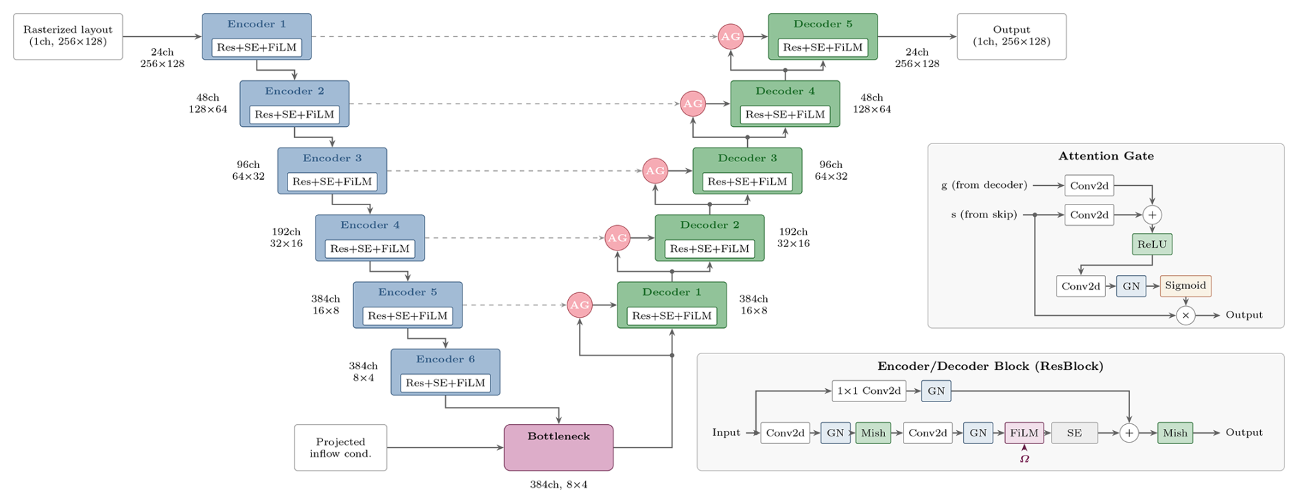
Figure 6 Overview of the attention residual U-Net (ARU-Net) architecture. The model follows an encoder–decoder structure with skip connections, incorporating squeeze-and-excitation (SE) attention in each block and attention gates (AG) on skip connections. Inflow conditions are injected at the spatial bottleneck and through feature-wise linear modulation (FiLM) layers.

Conditioning on inflow variables $\mathbf{\Omega }\in \mathit{\{}{U}_{\mathrm{\infty }},I_{\mathrm{0}}\mathit{\}}$ is achieved through two mechanisms. At the spatial bottleneck, the scalar inputs are projected to match the bottleneck channel dimension, broadcast across the spatial dimensions, and added to the feature map. This is followed by channel mixing using an expansion, followed by a compression pathway, such that the channels are expanded by $c\to \mathrm{2}c\to c$, with a residual connection and depthwise-separable spatial refinement. Additionally, FiLM layers modulate intermediate feature maps throughout the encoder (from the second block onward) and all decoder blocks:

$$\begin{array}{}\text{(6)}& \mathrm{FiLM}(\mathit{h},\mathbf{\Omega })=\mathit{h}\odot (\mathrm{1}+\mathit{\gamma }(\mathbf{\Omega }\left)\right)+\mathit{\beta }\left(\mathbf{\Omega }\right),\end{array}$$

where γ and β are learned scale and MLP scalers for the inflow conditions, with outputs clamped to ±0.3 and ±0.1, respectively, to ensure stable training. Regularisation is applied through dropout (10 % in the bottleneck and decoder) and stochastic depth with a linear schedule that increases from 0 % at the shallowest encoder block to a peak, determined during hyperparameter tuning, at the deepest encoder blocks and is mirrored symmetrically in the decoder.

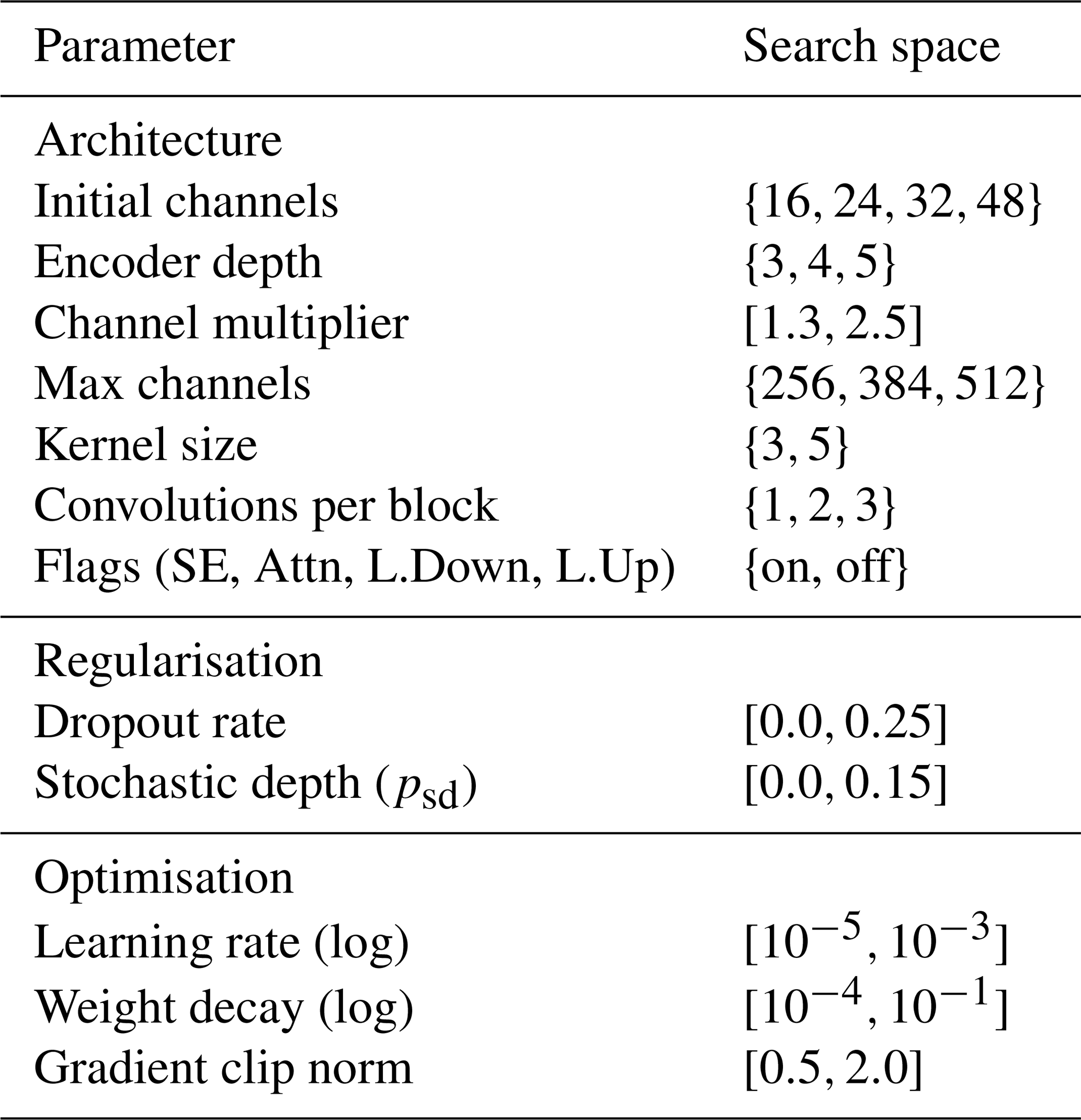
To select the ARU-Net architecture and training hyperparameters, a Bayesian hyperparameter optimisation was conducted on the TurbOPark engineering dataset using the Optuna framework (Akiba et al., 2019) with the tree-structured Parzen estimator (TPE) sampler. A total of 200 trials were evaluated, each trained for a fixed budget of 50 epochs. The final selected model was subsequently trained to convergence on the full TurbOPark dataset. The search space for the hyperparameter tuning can be seen in Table 2. A weight decay of 0.01 was applied through the AdamW optimiser, and gradients were clipped to a maximum norm of 1.0.

For the ARU-Net, the inflow conditioning variables are scaled to the unit interval via min–max normalisation: $U_{\mathrm{\infty }}\in [\mathrm{4.0},\mathrm{25.0}]$ m s⁻¹ and $I_{\mathrm{0}}\in [\mathrm{0.03},\mathrm{0.25}]$ are each mapped to [0, 1]. The target flow field undergoes a log-deficit transformation. Because RANS-AWF simulations can produce local speed-ups from blockage effects, cell velocities exceeding U_∞ are first clamped to U_∞. The relative wake deficit, $\mathit{\delta }=\mathrm{1}-u/U_{\mathrm{\infty }}$, then quantifies the fractional velocity reduction at each grid cell. Because the logarithm is singular at zero, a floor value ${\mathit{\epsilon }}_{\mathrm{0}}={\mathrm{10}}^{-\mathrm{5}}$ is applied, giving the clamped deficit ${\mathit{\delta }}_c=max(\mathit{\delta },{\mathit{\epsilon }}_{\mathrm{0}})$. The normalised target $\stackrel{\mathrm{̃}}{\mathit{\delta }}\in [\mathrm{0},\mathrm{1}]$ is then obtained as

$$\begin{array}{}\text{(7)}& \stackrel{\mathrm{̃}}{\mathit{\delta }}={\displaystyle \frac{\ln {\mathit{\delta }}_c-\ln {\mathit{\epsilon }}_{\mathrm{0}}}{-\ln {\mathit{\epsilon }}_{\mathrm{0}}}}.\end{array}$$

This log transformation compresses the wide dynamic range of wake deficits, improving the network's ability to resolve both strong and near-wake losses and subtle far-wake recovery.

Table 2 Hyperparameter search space for the ARU-Net architecture (15 dimensions). The search was conducted using the Optuna framework. Categorical choices are denoted by braces {…} and continuous ranges by brackets […].

2.6 Graph neural operator (GNO)

The GNN approach uses the GNO model, first introduced in Schøler et al. (2026). The GNO is a graph-based surrogate model that enables the prediction of flow fields. An overview of the model is presented in Fig. 7. The architecture is organised into three stages: an encoder (ℰ) that projects turbine features and their spatial relationships into a latent space, an approximator (𝒜) that iteratively refines turbine states through learned message passing, and a decoder (𝒟) that evaluates the resulting flow at arbitrary locations.

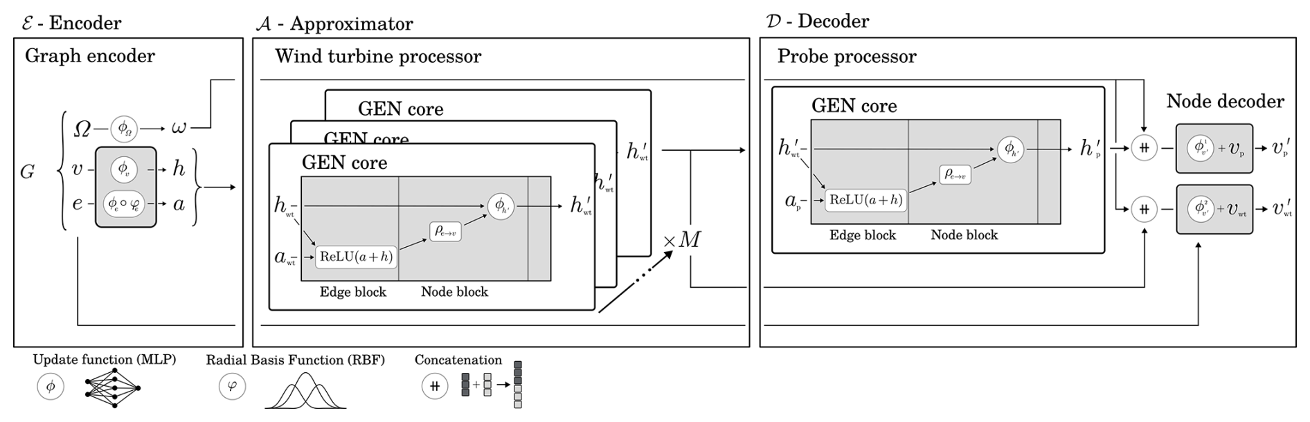
Figure 7 Overview of the GNO model with the added global context. The three main components remain encoder (ℰ), approximator (𝒜), and decoder (𝒟).

The architecture has one addition: a global context that supplies inflow conditions to the decoder, as illustrated in Fig. 7, following the path of Ω. Rather than concatenating the raw inflow values $\mathbf{\Omega }\in \mathit{\{}U,I_{\mathrm{0}}\mathit{\}}$ directly to the process node, which would mix observational and latent spaces, a small encoder ϕ_Ω first projects Ω into a latent representation ω with the same dimensionality as the latent space node features. Because its sole purpose is to bridge this dimensional mismatch, ϕ_Ω is implemented as a single-hidden-layer neural network,

$$\begin{array}{}\text{(8a)}& {\displaystyle }{\mathit{h}}_{\mathrm{\Omega }}^{\left(\mathrm{1}\right)}& {\displaystyle }={\mathit{\psi }}_{\mathrm{r}}\left({\mathbf{W}}^{\left(\mathrm{0}\right)\top }\mathbf{\Omega }+{\mathit{b}}^{\left(\mathrm{0}\right)}\right),\text{(8b)}& {\displaystyle }{\mathit{\varphi }}_{\mathrm{\Omega }}\left(\mathbf{\Omega }\right)& {\displaystyle }=\mathit{\omega }={\mathbf{W}}^{\left(\mathrm{1}\right)\top }{\mathit{h}}_{\mathrm{\Omega }}^{\left(\mathrm{1}\right)}+{\mathit{b}}^{\left(\mathrm{1}\right)},\end{array}$$

where ${\mathit{h}}_{\mathrm{\Omega }}^{\left(\mathrm{1}\right)}$ is the hidden-layer activation, and W^(l) and b^(l) are the learnable weights and biases of layer l. The resulting ω=ϕ_Ω(Ω) is concatenated to each process node prior to decoding. The remaining hyperparameter names are adopted directly from Schøler et al. (2026), with the latent space dimension (Q), hidden layer size of the internal MLP (q_int) and hidden layers (L_int), the number of message-passing steps in the wind turbine processor (M_wt) as seen in Fig. 7, and hidden layer size of the decoder (q_dec) and the decoder hidden layers (L_dec). To ensure that changes in both the data type and the model architecture are adequately addressed, a smaller grid search has been conducted with variations in these hyperparameters.

The GNO uses the normalisation and regularisation techniques from Schøler et al. (2026), normalising inputs and targets to the min–max range, applying dropout with a rate of 10 %, and using layer normalisation. In addition, during transfer learning, gradient clipping normalisation has been added as an optional addition, with a max l² norm of 1.0.

In Fig. 8 an overview of the data flow is provided, demonstrating how the model stages process the graph and a prediction is made. This design decouples the turbine interaction model from the spatial prediction, allowing new locations to be evaluated without recomputing the upstream turbine graph. A full description of the base architecture is given in Schøler et al. (2026). The remainder of this section describes an improvement introduced in the present work.

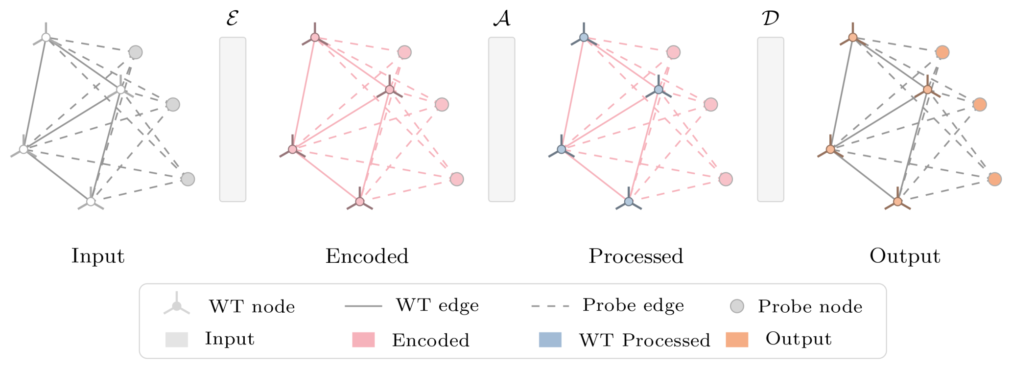
Figure 8 GNO model input and output augmentation. The model stages, encoder ℰ, approximator 𝒜, and decoder 𝒟, are displayed as simple blocks; see Fig. 7 for the expanded model stages.

To distinguish between the ARU-Net and the GNO, it is at times convenient to refer to the GNO with the operator notation, 𝒢. All considered model variations are based on the best original model, designated as 𝒢_org. In addition, three smaller and three larger models have been considered. These variations are reported here in order of size: 𝒢_S3, 𝒢_S2, 𝒢_S1, 𝒢_org, 𝒢_L1, 𝒢_L2, and 𝒢_L3. The actual model configurations are reported in Table 3. In addition, for the step-based learning rate schedule, two initial learning rates, $\mathrm{5}\times {\mathrm{10}}^{-\mathrm{3}}$ and $\mathrm{1}\times {\mathrm{10}}^{-\mathrm{3}}$, have been considered, each divided by 10 at 200 and 350 epochs, respectively.

2.7 Training and validation

For training the respective models, different stochastic gradient-based optimisers have been used: the GNO has been trained with Adam (Kingma and Ba, 2014) using default parameters, while the ARU-Net has been trained using AdamW (Loshchilov and Hutter, 2019), which decouples weight decay from the adaptive learning rate by applying it directly to the parameters, ensuring that regularisation is applied uniformly regardless of gradient history. For the GNO, training is monitored using the validation set, which is evaluated every five epochs. If an improvement of less than $\mathrm{1}\times {\mathrm{10}}^{-\mathrm{7}}$ is observed over 1000 consecutive epochs, training is stopped. During transfer learning to the RANS-AWF dataset, the limit is lowered to 200 epochs. The ARU-Net and GNO use slightly different training stacks. The ARU-Net is built on PyTorch (Paszke et al., 2019), while the GNO is built on a JAX-based framework (Bradbury et al., 2018), using Jraph (Godwin et al., 2020) for GNN abstractions, Flax (Heek et al., 2024) for neural network layers, and PyTorch Geometric (Fey and Lenssen, 2019) for graph construction and data loading. All training was done on a system featuring two AMD EPYC 7351 16-core CPUs (32 cores, 2.4 GHz), 256 GB of DDR4 RAM (2.666 GHz), and an 8 GB NVIDIA Quadro RTX 4000 GPU (Technical University of Denmark, 2019).

Performance metrics and loss function

During training and validation, two metrics are considered: the l¹-norm-based mean absolute error (MAE) and the l²-norm-based mean squared error (MSE). MSE is used as the loss function (ℒ) for both the ARU-Net and the GNO. In addition, during testing, the root mean squared error (RMSE) and an F₁ score are also reported. MAE and MSE are used to compare models during development, while RMSE is chosen for final evaluation as it is more readily interpretable than MSE. While most of these metrics are standard for flow surrogates, the F₁ score is less common. The F₁ score is typically used in classification tasks, where it quantifies performance by comparing true positives (t_p), false positives (f_p), and false negatives (f_n). Here, the F₁ score is used to evaluate how well the wake boundary is captured. A binary mask is created using a threshold (δ_w): grid points falling below the threshold are classified as unwaked and those above as waked. Equation 9 shows the definitions of the metrics applied in this paper:

$$\begin{array}{}\text{(9a)}& {\displaystyle }& {\displaystyle }\mathrm{MAE}={\displaystyle \frac{\mathrm{1}}{N}}{∥\mathit{u}-{\mathit{u}}^{\prime }∥}_{\mathrm{1}},\text{(9b)}& {\displaystyle }& {\displaystyle }\mathcal{L}=\mathrm{MSE}={\displaystyle \frac{\mathrm{1}}{N}}{∥\mathit{u}-{\mathit{u}}^{\prime }∥}_{\mathrm{2}}^{\mathrm{2}},\mathrm{RMSE}={\displaystyle \frac{\mathrm{1}}{\sqrt{N}}}{∥\mathit{u}-{\mathit{u}}^{\prime }∥}_{\mathrm{2}},\text{(9c)}& {\displaystyle }& {\displaystyle }{F}_{\mathrm{1}}={\displaystyle \frac{\mathrm{2}\cdot \mathrm{precision}\cdot \mathrm{recall}}{\mathrm{precision}+\mathrm{recall}}}={\displaystyle \frac{\mathrm{2}{t}_{\mathrm{p}}}{\mathrm{2}{t}_{\mathrm{p}}+f_{\mathrm{p}}+f_{\mathrm{n}}}},\end{array}$$

where u represents the target velocities, u^′ represents the predicted velocities, and N is the number of observations. The F₁ score, defined as the harmonic mean of precision and recall, is shown in two equivalent forms: one using precision and recall and one using the classification outcomes t_p, f_p, and f_n to emphasise its interpretation as an overall classification accuracy metric.

Multi-fidelity transfer learning

A range of different strategies has been tested to perform the transfer learning. The most straightforward approach is to update all weights during transfer learning; however, in some cases, this has been reported to be less efficient than freezing parts of the network during the transfer learning stage (Hu et al., 2021). Updating all parameters during transfer learning is termed fine-tuning, whereas freezing parts of the network is collectively referred to as weight freezing. Finally, the last considered approach is a variation of parameter-efficient fine-tuning (PEFT) called low-rank adaptation (LoRA) by Hu et al. (2021), which is referred to as LoRA fine-tuning. During fine-tuning with LoRA, the pre-trained weights ${\mathbf{W}}_{\mathrm{0}}^{\left(l\right)}\in {\mathbb{R}}^{d\times p}$ are frozen across the entire network. LoRA adapters are introduced in all layers of the targeted MLPs, while the remaining MLPs are kept fully frozen. For each adapted layer, the forward pass becomes

$$\begin{array}{}\text{(10a)}& {\displaystyle }& {\displaystyle }{\mathit{\xi }}^{\left(l\right)}=\left({\mathbf{W}}_{\mathrm{0}}^{\left(l\right)}+\mathrm{\Delta }{\mathbf{W}}^{\left(l\right)}\right){\mathit{\xi }}^{(l-\mathrm{1})},& {\displaystyle }\text{(10b)}& {\displaystyle }& {\displaystyle }\mathrm{\Delta }{\mathbf{W}}^{\left(l\right)}={\mathbf{B}}^{\left(l\right)}{\mathbf{A}}^{\left(l\right)},& {\displaystyle }\text{(10c)}& {\displaystyle }& {\displaystyle }{\mathbf{A}}_{\mathrm{0}}^{\left(l\right)}\sim \mathcal{N}(\mathrm{0},\mathrm{1}/r),{\mathbf{B}}_{\mathrm{0}}^{\left(l\right)}=\mathbf{0},& {\displaystyle }\end{array}$$

where ${\mathbf{A}}^{\left(l\right)}\in {\mathbb{R}}^{r\times d}$ and ${\mathbf{B}}^{\left(l\right)}\in {\mathbb{R}}^{p\times r}$, with a pre-determined rank r that controls the degree of parameter reduction. The initialisation in Eq. (10c) ensures ΔW^(l)=0 at the start of fine-tuning, so the model initially reproduces the pre-trained predictions exactly.

2.8 Testing and validation

To test the performance of the neural networks, a separate test set is used to avoid data leakage. While it is a moderate dataset of 200 inflow–layout combinations, it is still more than what is practical for creating qualitative plots, such as streamwise velocity deficit profiles and flow field plots. To ensure a representative sub-sample, the test set is grouped by layout size into three categories based on the number of turbines. Within each size category, three inflow conditions are selected targeting the diagonal of the (U_∞, I₀) space. The low, medium, and high regions are defined by dividing the wind speed and ambient TI ranges into three equal bins across all test cases. For each size–inflow combination, the case closest to the centroid of each category in the (U_∞, I₀) space is selected, yielding nine representative test cases in total. The three size categories are split into the following sizes (n_wt): small (S, n_wt≤47), medium (M, $\mathrm{47}<n_{\mathrm{wt}}<\mathrm{110}$), and large (L, n_wt≥110), where the S–M boundary is the median of sub-large layouts, and the M–L boundary is set at 110 turbines. These thresholds yield 21 small, 21 medium, and 8 large layouts. The selection of these regions is shown visually in Fig. 9.

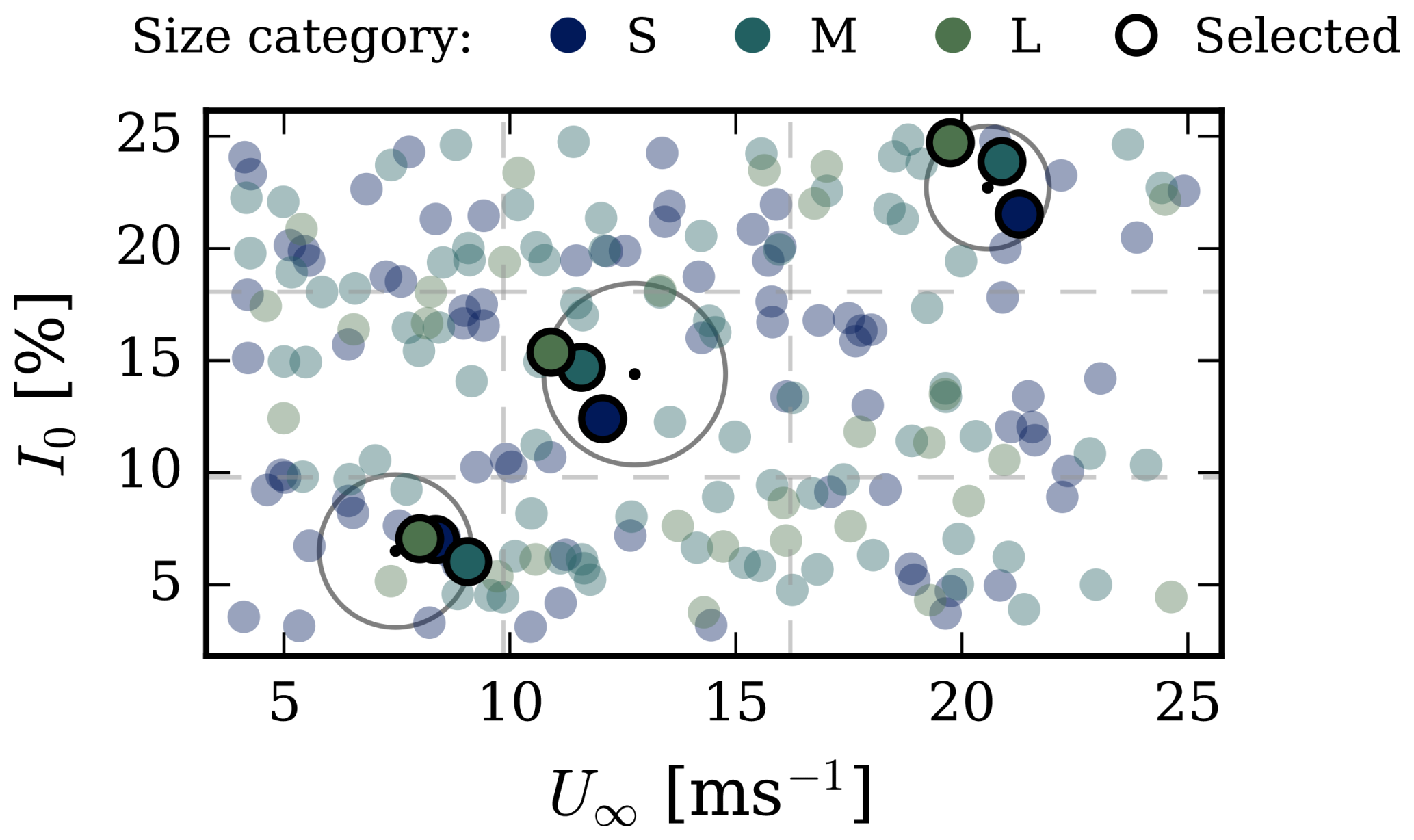
Figure 9 Selection of the RANS-AWF test subset for qualitative evaluation. Background scatter points represent the layouts in the test set, grouped by turbine count n_wt into S, M, and L. The parameter space of (U_∞, I₀) is divided into low, medium, and high regions along the diagonal. For each size category, the case closest to the centroid of each (U_∞, I₀) region is selected. The centroids of each background region are marked with a black dot, surrounded by a circle encompassing the three size-selected test cases.

For the transfer learning approach to be feasible, it is a prerequisite that the source and target domains share sufficient similarities for the learned representations to generalise, while the high-fidelity data remain sufficiently different that training on both provides meaningful improvements in accuracy, justifying the additional cost. Figure 10 examines that balance for the two fidelity levels used in this work, with Fig. 10a–d displaying the flow case from the RANS-AWF test dataset with the largest overall RMSE between TurbOPark and RANS-AWF (n_wt=185, U_∞=5.90 m s⁻¹, I₀=3.69 %).

Figure 10a shows the cross-stream velocity profiles, meaning the relative streamwise velocity deficit $\mathrm{\Delta }u/U_{\mathrm{\infty }}$ across the lateral y direction, at specific downstream x locations. It shows that, even in this worst-case scenario, the two models share broad structural similarities. Overall, the wind farm wake expansion and extent of the wake region are consistent between TurbOPark and RANS-AWF. However, TurbOPark generally overestimates the magnitude of the wake deficit compared to RANS-AWF (Fig. 10a, f), consistent with earlier findings that TurbOPark predicts stronger wind farm wake effects than RANS (van der Laan et al., 2023). The individual turbine wakes in TurbOPark also remain distinctly separated, especially for low TI, where the turbulent mixing is at a minimum, producing a jagged cross-stream profile, whereas the RANS-AWF solution shows significantly greater lateral mixing that merges neighbouring wakes into a smooth deficit profile. The two-dimensional velocity maps (Fig. 10b–c) confirm these observations. TurbOPark retains a jagged wake structure for all downstream distances, while the RANS-AWF field is laterally diffused a few rotor diameters downstream. From Fig. 10d, it can further be seen that the RANS-AWF dataset contains blockage upstream of the wind farm and speed ups on the side of the wind farm.

This has implications for the ARU-Net target representation, since velocities above U_∞ are clamped to U_∞ before the logarithmic wake deficit transformation. The ARU-Net is not trained to reproduce these local speed-up regions, whereas the GNO predicts velocity directly and is not subject to the same target-space restriction. This is, however, expected to have limited influence on the threshold-based wake metrics reported below, since the wake mask is defined using ${\mathit{\delta }}_{\mathrm{w}}\ge {\mathrm{10}}^{-\mathrm{3}}$, while clamped speed-up and unwaked regions are assigned the much smaller floor value ${\mathit{\epsilon }}_{\mathrm{0}}={\mathrm{10}}^{-\mathrm{5}}$. The effect is therefore mainly relevant for full-field error comparisons and for applications in which blockage-induced acceleration is of interest.

The quantile-to-quantile density scatter of the wake region (Fig. 10e) quantifies this difference, giving an RMSE of 1.31 %, an MAE of 0.48 %, and a coefficient of determination of R²=0.47. The low R² indicates that, despite the broad similarities between the wakes, the two models differ significantly in the pointwise magnitudes of the predicted wake deficits. The mean streamwise wake recovery curves (Fig. 10f) further illustrate this difference. The lateral average wake deficit calculated by TurbOPark is consistently larger than the RANS-AWF reference downstream of the wind farm. From Fig. 10f, it can also be observed that the RANS-AWF model includes decreased wind speed upstream from the wind farm due to blockage.

Finally, the RMSE between the two models, binned by the free-stream velocity and ambient TI (Fig. 10g), shows a clear dependency on the inflow conditions. The largest difference between the two models occurs at low wind speeds and low I₀, where high thrust coefficients increase the individual wake deficits and reduce turbulent mixing, thereby limiting both turbulent mixing and streamwise recovery. Especially at wind speeds below 13 m s⁻¹, the difference between TurbOPark and RANS-AWF is most significant.

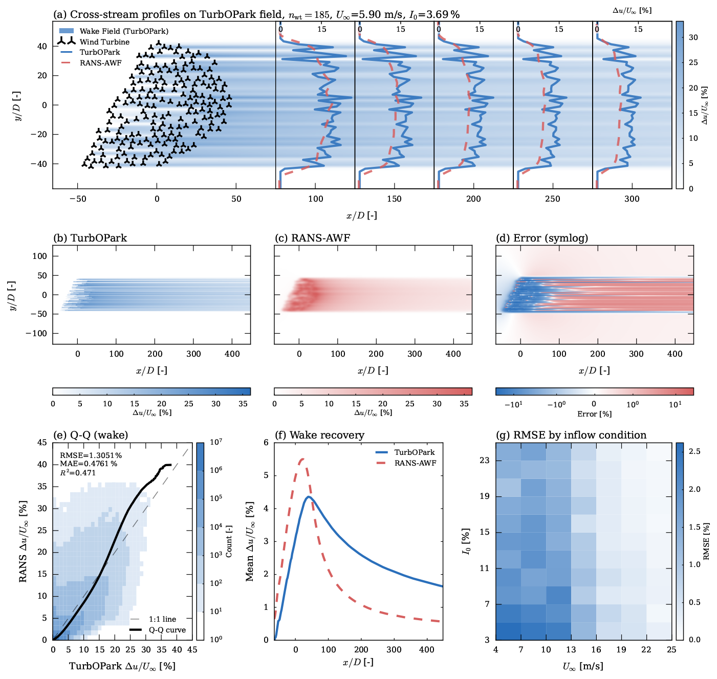
Figure 10 Comparison between TurbOPark and RANS-AWF. (a) Cross-stream velocity profiles ($\mathrm{\Delta }u/U_{\mathrm{\infty }}$). (b–c) Two-dimensional maps of $\mathrm{\Delta }u/U_{\mathrm{\infty }}$ for an arbitrary case. (d) Spatial difference map ($\mathrm{\Delta }u/U_{\mathrm{\infty }}$) on a symmetric logarithmic scale. (e) Quantile-to-quantile density scatter of effective velocity in the wake region, with RMSE, MAE, and R². (f) Streamwise wake recovery as laterally averaged $\mathrm{\Delta }u/U_{\mathrm{\infty }}$ versus $x/D$. (g) RMSE between models binned by freestream wind speed and turbulence intensity (I₀).

3 Results and discussion

This section first presents the results of the architecture search for engineering-model-based source models, followed by the transfer learning results. Based on these, the best-performing ARU-Net and GNO models are selected and analysed together in terms of prediction accuracy and ability to resolve the wake region of the flow. This analysis comprises both a qualitative comparison, using cross-stream velocity deficit plots and flow field plots of velocity predictions from both models, and a quantitative comparison of performance metrics.

3.1 Engineering source model – architecture search

To investigate the effect of model architecture, a small hyperparameter search was performed for both the ARU-Net and the GNO. The best configuration from the ARU-Net hyperparameter search (Table 2) uses five encoder levels with channel counts of 24, 48, 96, 192, and 384, yielding 16 113 456 parameters. The optimiser enabled SE blocks, AGs, and learnable downsampling but preferred transposed convolutions (2×2 kernels, stride 2) over the bilinear-plus-learned-convolution alternative for upsampling. Training uses an effective batch size of 32 (physical batch size of 8 with 4 gradient accumulation steps), 16 bit floating-point mixed-precision arithmetic, and no learning rate schedule. When trained to converge on TurbOPark, the selected model achieves a full-domain RMSE of 0.1050 m s⁻¹ and MAE of 0.0225 m s⁻¹ on the validation set. Table 3 shows the results of this search.

Table 3 Source model architecture search on TurbOPark dataset, evaluated on validation set. The ARU-Net architecture was selected via a 200-trial Optuna search (Table 2); the GNO results show the best result per architecture across 14 configurations (7 architectures × 2 initial learning rates). Best value per metric column in bold.

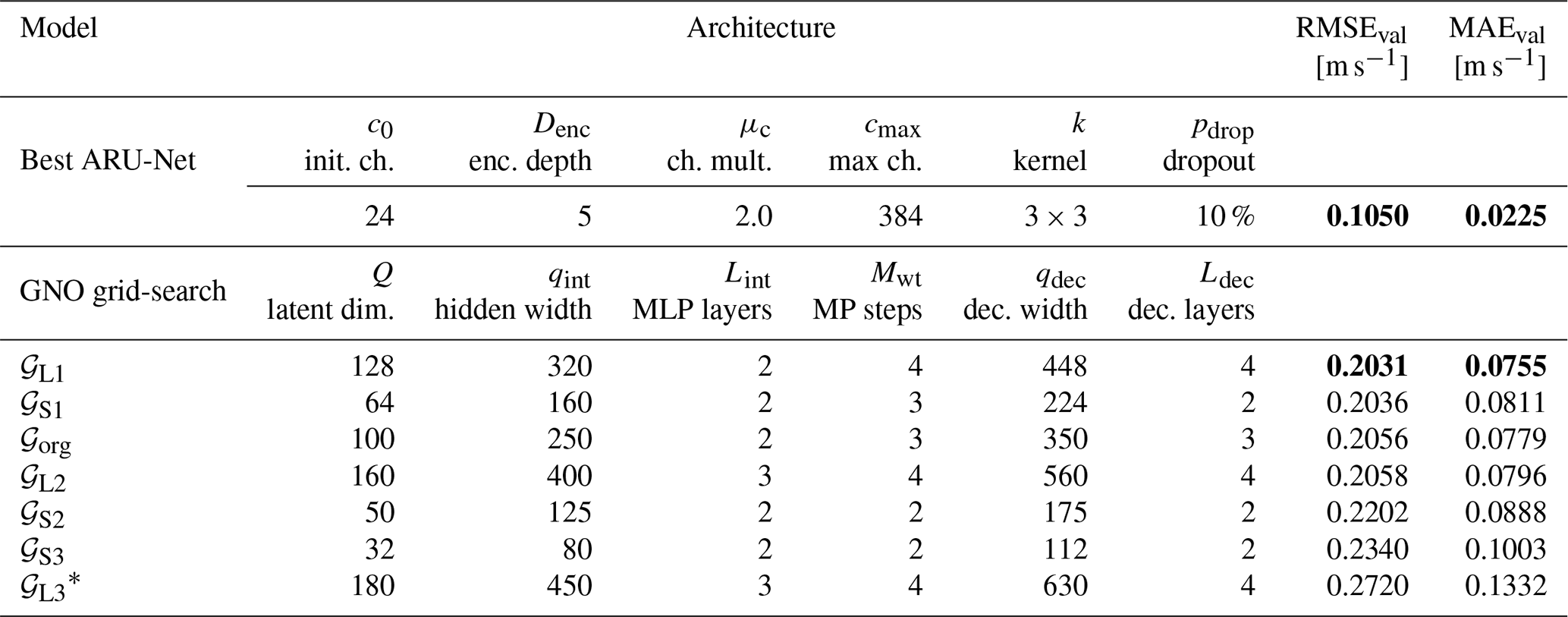
^* Best result obtained with initial learning rate 10⁻³.

For the GNO, a simple grid search was conducted, as described in Sect. 2.6, and seven model variations were considered. The two best-performing GNO configurations are the variations closest to the originally best 𝒢_org configuration described in Schøler et al. (2026), namely the 𝒢_L1 and 𝒢_S1 models, followed by the 𝒢_org setup itself. The best-performing 𝒢_L1 model uses slightly larger internal and decoder MLPs and employs four wind turbine message-passing steps (M_wt) instead of the original three. The hyperparameter tuning done during the creation of the TurbOPark pre-trained model is not exhaustive. A more thorough tuning could yield baseline models that yield better metrics. However, the authors believe that improvement would be minor.

3.2 Transfer learning – RANS-AWF hyperparameter search

Based on the results of the initial source model training stage, a transfer learning experiment is conducted using combinations of the different approaches described in Sect. 2.7 with the chosen model architectures. The ARU-Net model architecture was selected as the best-performing model from the hyperparameter tuning on the TurbOPark dataset, as described in Sect. 2.5. The resulting hyperparameters for the ARU-Net are shown in Table 3. Before the model was used as the initial weights for the fine-tuning procedures, it was further trained to convergence, beyond the initial 50 epochs. This model is denoted as ARU-Net Best in Table 3. During fine-tuning, the exact same model architecture and hyperparameters were used as during the pre-training, except for the learning rate, which was tested for $\text{lr}\in \mathit{\{}{\mathrm{10}}^{-\mathrm{5}},{\mathrm{10}}^{-\mathrm{4}},{\mathrm{10}}^{-\mathrm{3}},{\mathrm{10}}^{-\mathrm{2}}\mathit{\}}$. For the LoRA-fine-tuned models, each learning rate was tested with ranks $r\in \mathit{\{}\mathrm{4},\mathrm{8}\mathit{\}}$. The GNO was tested across a range of transfer learning combinations, using 𝒢_L1 as the source model. As a significant number of variations were included, the models have been grouped into categories, and only the best in each group are shown in Table 4.

Table 4 Results of RANS-AWF transfer learning for both the ARU-Net and the GNO. The GNO results are based on the best L1 model weights from the TurbOPark training. Results are grouped by architecture and fine-tuning strategy, showing only the best configuration per category. N is the number of models in each category. Best model options, listing the learning rate, the LoRA rank and α where applicable, as well as the gradient clipping setting for the GNO. All models are trained on an Nvidia Quadro P4000 GPU. GNO metrics are reported to five decimal places to distinguish otherwise tied values. Best metrics are marked with bold.

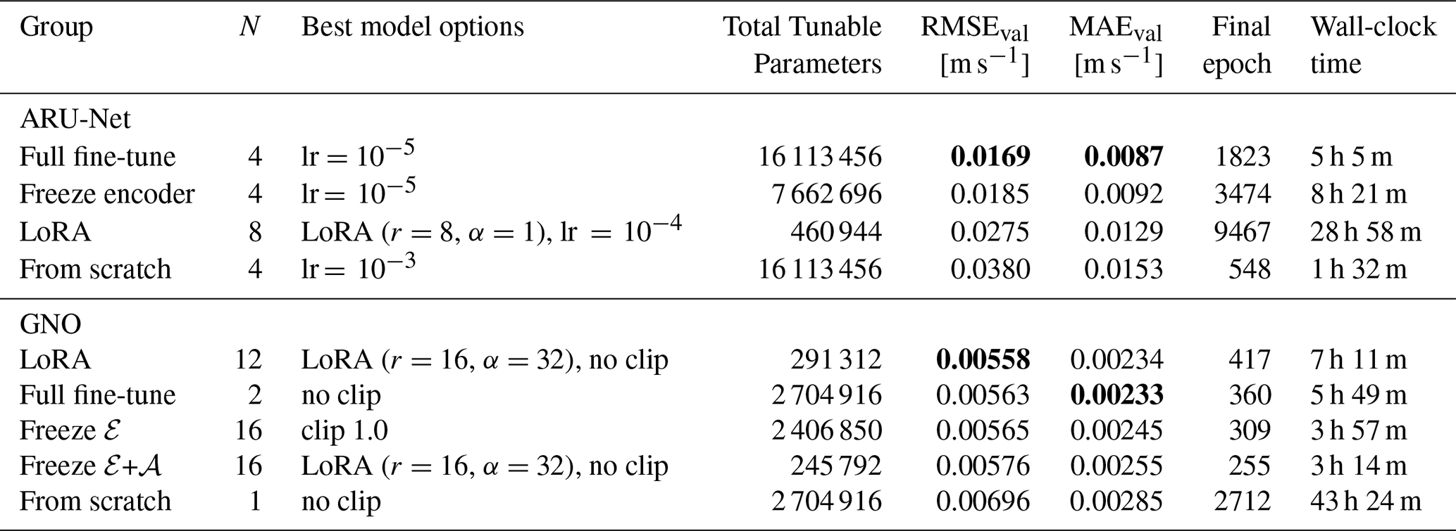
As shown in Table 4, for both the ARU-Net and GNO, the LoRA-based approach yields no significant computational advantage over full fine-tuning or training from randomly initialised weights, despite the reduction in tunable parameters. This is likely because the full models are relatively small, leading the training process to be dominated by overhead, or because the ratio of tunable parameters in the LoRA configuration relative to the full model is not as distinct as in large language models (LLMs) with billions of parameters. For the ARU-Net, the fully fine-tuned model and the frozen-encoder variant perform comparably, whereas LoRA and training from scratch perform worse. This indicates that initialising the model weights and leaving them fully or partially tuneable is the most effective strategy, as it leverages the pre-learned wake physics while retaining sufficient flexibility to adapt to the high-fidelity data, unlike the restricted parameter space of LoRA or the uninformative starting point of random initialisation.

Table 4 shows that for the majority of the fine-tuning techniques used for fine-tuning the GNO, the results fall within an acceptable range. Even for the model, which is trained from scratch using randomly initialised parameters, the results are mostly acceptable. Interestingly, the full fine-tune group, which applies neither LoRA nor freezing, performs remarkably well, achieving the lowest MAE. Ultimately, the best model was a LoRA variant, but not by a wide margin. Although this improvement is smaller than that observed for the ARU-Net, it should not be interpreted as negligible. Compared with training the GNO from scratch, the best LoRA fine-tuned GNO reduces the validation RMSE from 0.00696 to 0.00558 m s⁻¹, corresponding to an improvement of approximately 20 %. Pre-training thus still provides the best absolute GNO performance, even though the relative benefit is more marginal than for the ARU-Net.

Another intriguing insight is that the time column in Table 4 shows that using LoRA did not significantly reduce training time compared to simply using the full fine-tuning variations. This indicates that wall-clock time is not solely determined by the number of trainable parameters. The frozen layers must still be evaluated in the forward pass, and for the GNO, additional overhead arises from graph batching, graph construction, and data loading. Therefore, LoRA mainly reduces the cost of gradient updates and optimiser states while leaving a substantial part of the per-epoch computation unchanged. This likely explains why the reduction in trainable parameters does not translate into a proportional reduction in wall-clock time. It should be noted that the reported wall-clock times are not intended as a hardware- or framework-normalised benchmark between ARU-Net and GNO, since the two models are implemented in different software stacks. The ARU-Net is implemented in PyTorch, whereas the GNO uses JAX, Jraph and Flax together with PyTorch Geometric for graph construction and data loading. The timing comparison should therefore mainly be interpreted within each architecture, where the same framework and data pipeline are used across fine-tuning strategies. The LoRA group coming out ahead is therefore ascribed to the fact that 12 configurations were considered, and one of the initialisations managed to escape a local minimum that the full fine-tuning runs became trapped in before early stopping was triggered. This interpretation is supported by the fact that only one LoRA model outperformed the best full fine-tuning model.

3.3 Qualitative study – predictions with representative layout–inflow cases

The streamwise coordinate x is measured from the centre of the wind farm, as seen in Fig. 5. The distance from the most downstream turbine to a given wake location varies with wind farm size. To account for this, we introduce $\stackrel{\mathrm{̃}}{x}$, defined as the streamwise distance from the most downstream turbine to that location. In Fig. 11, the nine selected combinations of farm layouts and inflow conditions described in Sect. 2.8 are used to create cross-stream deficit profiles at $\stackrel{\mathrm{̃}}{x}=\mathrm{6}D$ downstream distances for both predictions using the ground truth RANS-AWF data and the ARU-Net and GNO.

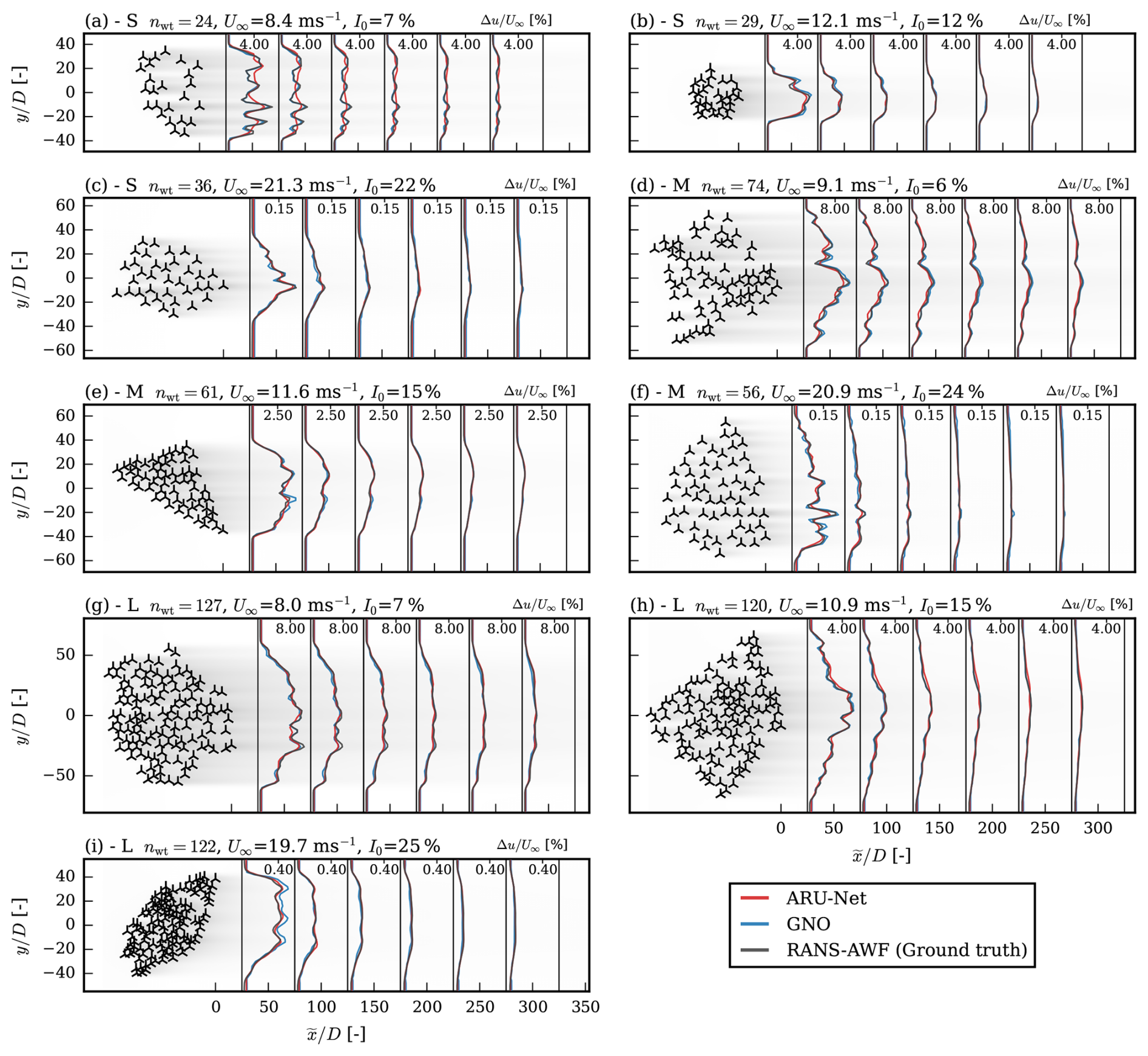
Figure 11 Cross-stream velocity deficits at selected distances behind the wind farm, comparing ARU-Net and GNO predictions against the RANS-AWF ground truth for a number of (a–c) small (S), (d–f) medium (M), and (g–i) large (L) farm layouts. Transverse profiles are extracted at downstream distances $\stackrel{\mathrm{̃}}{x}\in \mathit{\{}\mathrm{50},\mathrm{100},\mathrm{150},\mathrm{200},\mathrm{250},\mathrm{300}\mathit{\}}D$, where $\stackrel{\mathrm{̃}}{x}$ is measured from the turbine furthest downstream. The grey hue indicates the RANS-AWF flow field data.

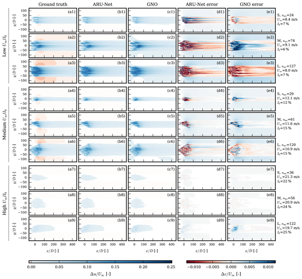
Figure 11 shows that both models produce good results and reproduce the ground truth with only minor inaccuracies. The areas where the ARU-Net has its most significant errors are dominated by a degree of over-smoothing, which is most notable in Fig. 11a at $\stackrel{\mathrm{̃}}{x}=\mathrm{50}D$, where the most significant relative discrepancy occurs. For the GNO, the error characteristics are not over-smoothing but rather a failure to capture the peak values accurately, primarily manifested as overestimation of peaks, e.g. as in Fig. 11e, i. In Fig. 12, the model predictions and ground truths are displayed as velocity field plots, with inclusions of model errors (ε). It is clear that both models perform worst in or near the farm. Simultaneously, there is a negative correlation between error and both free-stream velocity and ambient TI. This inverse correlation is due to wake physics: when the velocity is low, the turbines operate at high thrust coefficients, meaning they are in the state where they most affect the flow. At the same time, a low ambient TI means wake recovery is slow, as insufficient turbulence-induced mixing makes the wakes more persistent. These factors, when combined, produce a pronounced wake effect and a complex flow, both of which negatively affect model performance. That said, all investigated cases remain well within an acceptable error range for both models.

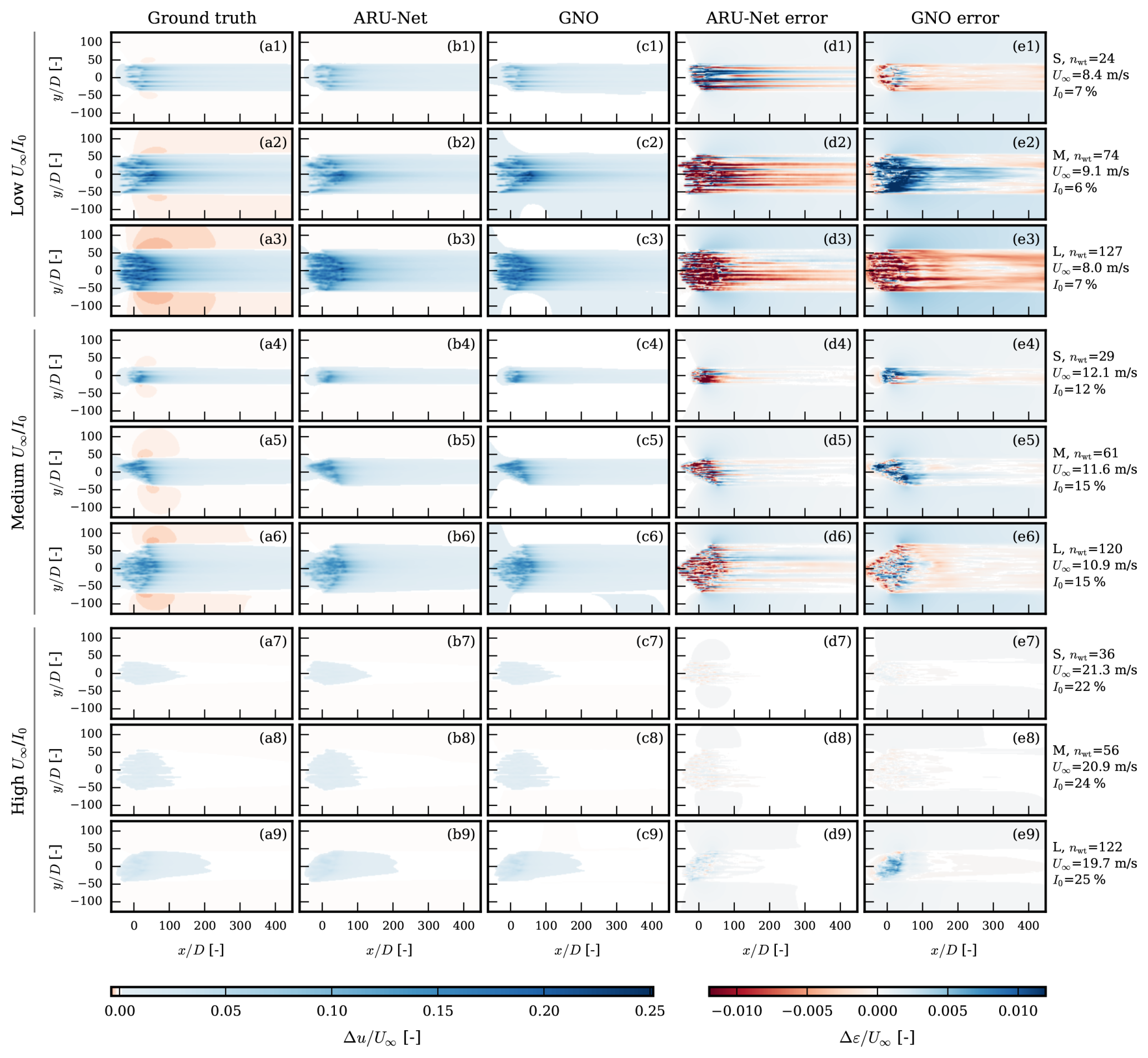
Figure 12 Flow field plots of the representative farm layout–inflow combinations. Columns indicate (a) RANS-AWF ground truth, (b) ARU-Net predictions, (c) GNO predictions, (d–e) free-stream normalised model errors for the ARU-Net and GNO, respectively.

For the ARU-Net, another behaviour has been identified. It is clearest in the case of the small wind farm at low wind speed: when the turbines are placed far apart, and the farm is small, there is a low degree of wake mixing, and the convolutional kernels are not sufficient to resolve the finer details of the flow. This is observed mainly in areas where a neighbouring wind farm would not be placed, but it remains an interesting qualitative difference between the considered models. For the GNO, there are indications of a similar behaviour, though it is less pronounced. When the farm is dense, as in Fig. 11b and e, the GNO tends to overestimate the wake effect slightly, although the effect is not clear enough to draw a decisive conclusion.

To facilitate a direct visual comparison between the two models, their absolute errors are subtracted for each of the representation layout–inflow combinations. The resulting difference fields are shown in Fig. 13, where blue indicates that the ARU-Net has lower error, and red indicates that the GNO has lower error.

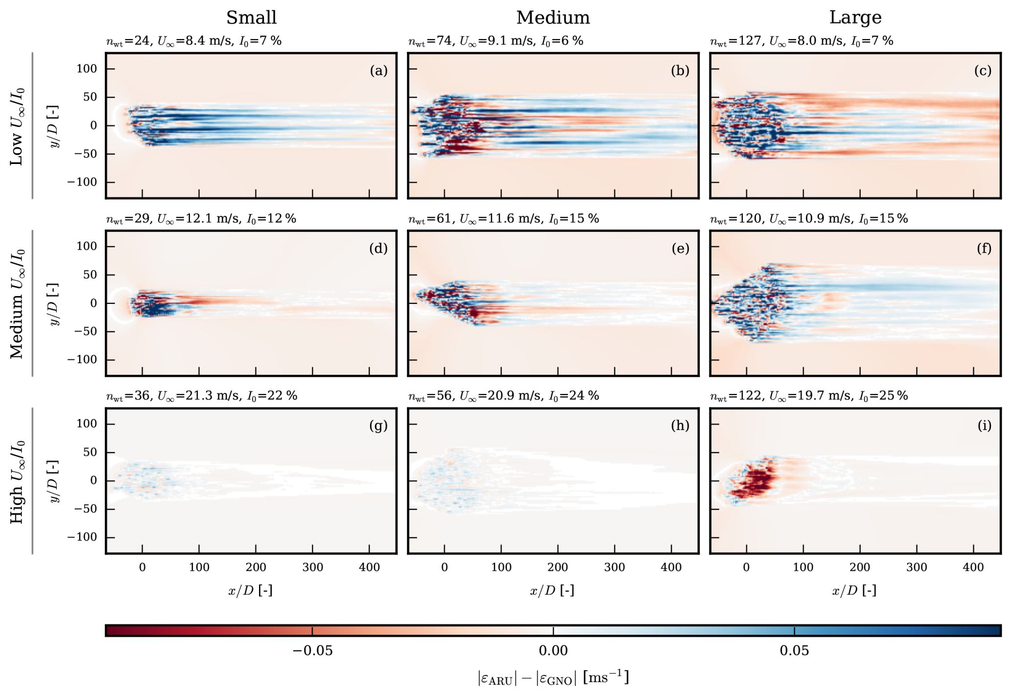
Figure 13 Model comparison using flow field error plots of the selected layout–inflow combinations.

As seen in Fig. 13, the relative difference between the models is low, and both models have areas where they outperform the other. Most notably, the ARU-Net performs slightly better in the L–high case (U_∞=19.7 m s⁻¹, I₀=25  %; Fig. 13i), while the GNO performs better in the S–low case (U_∞=8.4 m s⁻¹, I₀=7  %; Fig. 13a). Looking at the overall picture, the GNO appears to have a slight advantage over the ARU-Net, with more areas coloured red than blue. Also, the case where the ARU-Net performs best is with a high inflow velocity and a small nominal error, while the case where the GNO performs best is with a low velocity and a larger nominal error. However, because this advantage is primarily within the farm, it is not expected to yield a meaningful benefit in most practical applications.

3.4 Quantitative study – performance metrics and sensitivity analysis

To supplement the more qualitative investigation of the selected representative layout–inflow combinations, a quantitative comparison has been performed using the performance metrics introduced in Sect. 2.7. As a CNN-based approach requires a fixed, gridded domain, there will naturally be a lot of data with uninteresting flow, with no wake effect. This fixed-raster representation also affects evaluations away from the native CNN grid. When ARU-Net predictions are evaluated on the GNN grid in Table 5, the predictions are mapped from the native 256×128 CNN grid using bilinear interpolation. The degradation observed on the GNN grid, therefore, reflects both interpolation error and the fact that the ARU-Net is trained to output on a fixed raster. This is a practical limitation when predictions are required at arbitrary query locations that do not align with the training grid. In such cases, interpolation, retraining at the target resolution, or a grid-invariant architecture is required. By contrast, the GNO can evaluate arbitrary probe locations directly. While this area is partially of interest as a model should not predict strong wake effects where none are present, having it dominate the performance metrics is suboptimal. Therefore, the performance metrics are also reported using a range of wake masks (${\mathit{\delta }}_{\mathrm{w}}\in \left\{{\mathrm{10}}^{-\mathrm{5}},{\mathrm{10}}^{-\mathrm{4}},{\mathrm{10}}^{-\mathrm{3}}\right\}$ m s⁻¹) that have been applied on the RANS-AWF, and only the data above the threshold have been considered in the metric evaluation. The resulting performance metrics are reported in Table 5, along with the change in each metric relative to a TurbOPark reference. Please note that this metric is strictly included as a reference point and is not suitable for passing judgement on the TurbOPark model, as it was not calibrated towards RANS-AWF data.

Table 5 CNN (ARU-Net) vs. GNN (GNO) comparison across grids and wake deficit thresholds. Bilinear interpolation is used on the ARU-Net predictions when evaluating them on the GNN grid. Percentages in parentheses are relative changes compared to a TurbOPark baseline; for RMSE and MAE, negative values indicate an improvement, while for the F₁ score, a positive value indicates an improvement over the baseline. Best metrics are marked with bold.

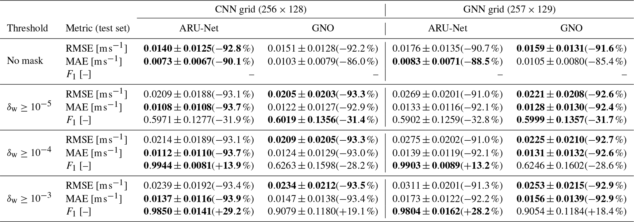
Table 5 shows a mixed picture of both the ARU-Net and the GNO performing well in different categories. To summarise these results with a single pair of metrics, the wake region (${\mathit{\delta }}_{\mathrm{w}}\ge {\mathrm{10}}^{-\mathrm{3}}$ m s⁻¹) grid-averaged RMSE is 0.024 m s⁻¹ for the GNO and 0.028 m s⁻¹ for the ARU-Net, while the corresponding F₁ scores are 0.91 and 0.98, respectively. However, both models achieve better performance when evaluated on grids matching the resolution of their respective training data. The GNO has the lowest RMSE in most scenarios, while the ARU-Net has the best F₁ score most of the time. This underpins the observations from the qualitative study, which found that the GNO performs slightly better in overall accuracy, while the ARU-Net captures the wake boundary more accurately. The ARU-Net's ability to capture a well-defined wake boundary may be due to logarithmic scaling of the target data, which emphasises smaller values and rewards the network for capturing these changes. Both models outperform the TurbOPark baseline across all cases, with lower RMSE and MAE. For the F₁ score, however, the ARU-Net only outperforms the baseline once the wake cut-off is set to $d_{\mathrm{w}}\ge {\mathrm{10}}^{-\mathrm{4}}$; at $d_{\mathrm{w}}\ge {\mathrm{10}}^{-\mathrm{5}}$, its performance drops off sharply. This drop-off is not practically significant: at the 10⁻⁵ level, the wake deficit cannot be distinguished from background variation under real conditions, so poor classification in this regime has little bearing on real-world performance. This supports the use of a more aggressive cut-off when applying the models.

To better understand how the models perform as input variables change, metrics are computed for each layout–inflow combination in the full test set. This is explored in Fig. 14, where the RMSE is binned by the different input variables, illustrating how the error behaves for the two considered models and for their variations trained from scratch during the transfer learning study. Figure 14 presents a comparison between the best-performing fine-tuned ARU-Net models and equivalent models trained without weight initialisation. The results indicate that the ARU-Net benefits significantly from pre-training compared to the GNO, with the RMSE often reduced by more than half in specific regimes. These improvements are most pronounced at wind speeds near the rated velocity ($U_{\mathrm{\infty }}\in [\mathrm{10},\mathrm{15}]$ m s⁻¹), in the lower-turbulence-intensity range ($I_{\mathrm{0}}\in [\mathrm{3},\mathrm{8}]$ %), and within the largest ($n_{\mathrm{wt}}\in [\mathrm{70},\mathrm{190}]$) and densest ($s_{\mathrm{wt}}/D\in [\mathrm{3},\mathrm{7}]$) wind farms. In contrast, the GNO only minimally benefits from transfer learning, showing only slight improvements or, in some instances, slightly degraded performance.

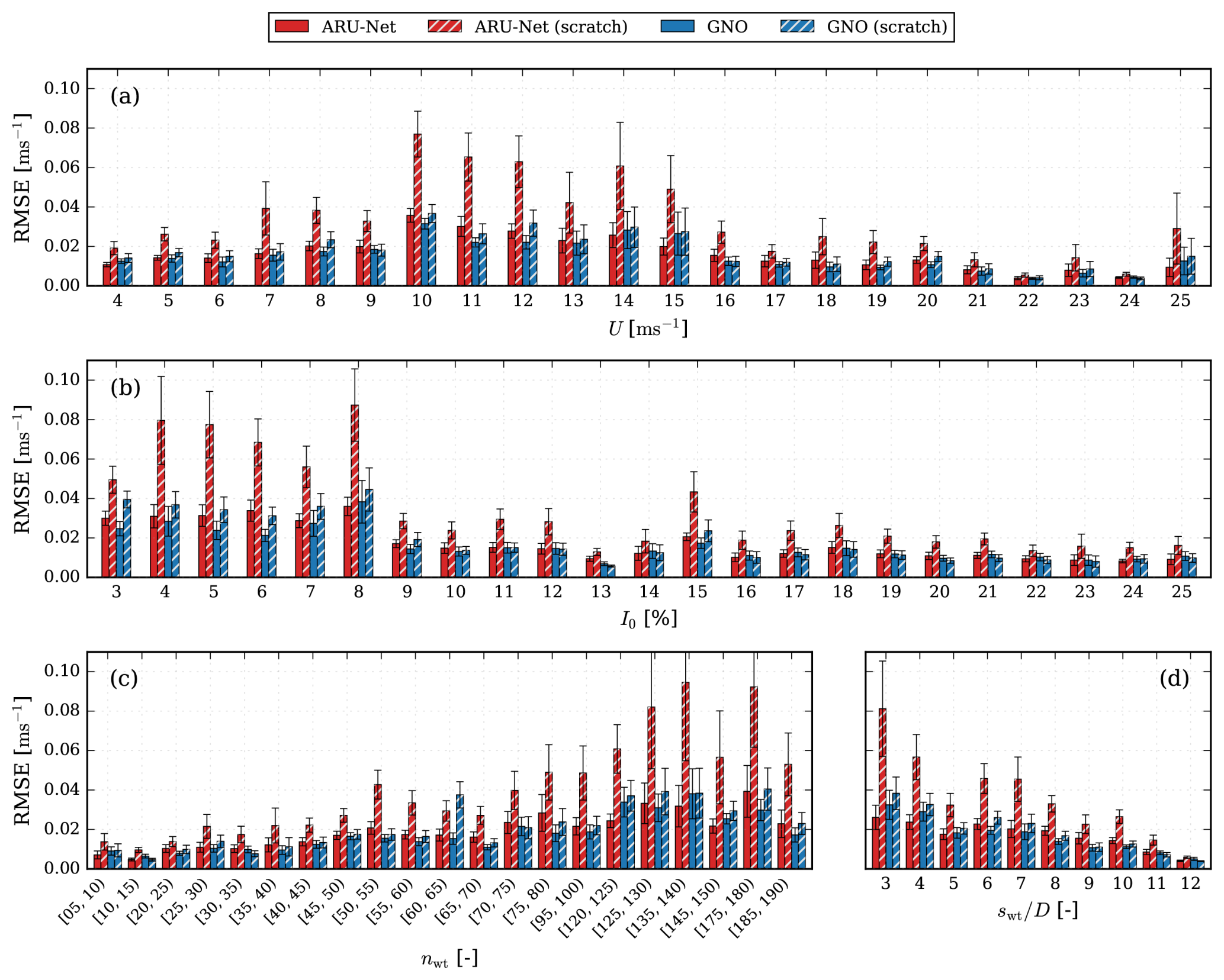
Figure 14 ARU-Net and GNO binned RMSE metrics with respect to inputs: (a) free-stream velocity U_∞, (b) ambient TI I₀, (c) number of wind turbines n_wt, and (d) wind turbine separation factor s_wt.

While more rigorous experimentation would be required to ascertain the precise cause of this behaviour, a plausible explanation is the structural differences between the two architectures. The GNO operates on an input–output graph whose nodes correspond to physical turbine positions, meaning the farm layout is encoded directly in the data representation fed to the model. The ARU-Net also receives layout information via a raster representation, which is propagated across the encoder and decoder stages via skip connections. However, this constitutes a weaker form of spatial enforcement than the explicit node-wise correspondence of the GNO graph. This stronger geometric inductive bias in the GNO may allow it to learn the underlying flow physics more effectively from limited high-fidelity data, reducing its dependence on low-fidelity pre-training and explaining the comparatively modest gains it achieves through transfer learning. From Fig. 14, it is clear that the ARU-Net trained from scratch performs much worse than any of the other models. It is, however, less clear whether the fine-tuned ARU-Net or GNO model performs better, though the GNO appears to have a slight edge, consistent with its lower RMSE in most scenarios in Table 5. It is important to note that the main objective of this work was to evaluate the ARU-Net and the GNO in capturing the inter-farm effects simulated by the reference RANS-AWF dataset, rather than demonstrating that these predicted wake deficits are comparable to those generated by large wind turbine clusters in practice. The RANS-AWF dataset is limited to the capabilities of both RANS and the conditions simulated. As mentioned previously, inter-farm wake effects can be highly influenced by large-scale atmospheric variability. Therefore, we also plan to extend the evaluation of the methods proposed in this work to account for the range of multiscale phenomena encountered by offshore wind farms.

3.5 Future work

The models presented in this work show great promise, and several avenues for further development have emerged. Drawing on the complementary strengths of each architecture, one promising direction is to use the ARU-Net's superior capability to characterise the wake region as a spatially informed background field for the GNO, replacing the current uniform background-flow assumption. This hybridisation could enable the GNO to match the ARU-Net in wake boundary prediction accuracy, as both models are already orders of magnitude faster than full RANS-AWF. This additional inference cost is not expected to be problematic. Another related direction is to investigate graph-transformer models, which may provide a more flexible attention-based mechanism for capturing long-range inter-turbine interactions while retaining the layout adaptability of graph-based surrogates. Alternatively, a more specialised ARU-Net could be trained exclusively to capture the wake boundary, potentially surpassing the current capability demonstrated here. From the ARU-Net perspective, the neural operator framework could be adopted by replacing the current convolutional kernels with Fourier layers similar to those in Fourier neural operator (FNO) networks, potentially improving generalisation to unseen spatial configurations. Finally, the scope of the training data could be broadened in several directions: extension to three-dimensional flow fields; inclusion of C_T curves to account for multiple turbine types; use of higher-fidelity full RANS simulations; and incorporation of more complex atmospheric conditions such as Coriolis force, atmospheric stability, and mesoscale effects.

4 Conclusions

This work presents a systematic comparison between an ARU-Net and a GNO as surrogate models for inter-farm wake deficit predictions. Both architectures were pre-trained on low-fidelity TurbOPark engineering model data and fine-tuned on high-fidelity RANS-AWF simulations using a multi-fidelity transfer learning strategy, though the GNO benefited only marginally from this approach. Both architectures have demonstrated strong capability to predict downstream wake deficits across a wide range of arbitrarily generated wind farm layouts and randomly generated ambient wind speed and turbulence intensity. The two models have shown complementary strengths: evaluated over the wake region (${\mathit{\delta }}_{\mathrm{w}}\ge {\mathrm{10}}^{-\mathrm{3}}$ m s⁻¹) and averaged across both evaluation grids, the GNO achieves a lower RMSE (0.024 vs. 0.028 m s⁻¹), indicating slightly better accuracy in estimating the flow field wind speed, while the ARU-Net attains a higher F₁ score (0.98 vs. 0.91), indicating a better ability to correctly predict wake boundaries. The advantage of the ARU-Net for predicting wake boundaries may be attributed to its logarithmic target transform, which improves its ability to estimate wake deficits across different magnitudes by equally rewarding the ARU-Net's ability to predict subtle and strong wake effects. However, this transformation does not preserve speed-up regions, so applications requiring accurate blockage-induced acceleration would require a modified target representation.

Qualitative analysis has revealed distinct failure modes for each network architecture. The ARU-Net is prone to over-smoothing its predictions, particularly for sparse wind farms with large turbine spacing, where the convolutional kernel was insufficient to resolve fine flow structures. In contrast, the GNO tended to overestimate peak wake deficits, most notably in dense wind farm configurations. Both models perform worst at low wind speeds and low ambient TI, consistent with the underlying wake physics: these conditions are dominated by high thrust coefficients and low turbulent mixing, leading to stronger, more persistent, and more complex wake structures, which are inherently more difficult to predict.

The transfer learning results demonstrate that the ARU-Net benefits substantially more from pre-training on engineering models than the GNO, with RMSE reductions often exceeding 50 % in specific regimes compared to training from scratch. In contrast, the GNO shows a smaller improvement from transfer learning than the ARU-Net, though it still achieves its best performance with it. This suggests that its intrinsic graph structure, where nodes directly represent physical turbines, and edges encode positional relationships, already provides a strong inductive bias for learning wake interactions even with limited high-fidelity data. For the ARU-Net, full fine-tuning and the frozen-encoder strategy performed comparably. Neither the ARU-Net nor the GNO improved from LoRA-based PEFT, which offered no significant computational or accuracy benefit over training from scratch, likely due to the relatively small size of the models compared to the large language models for which LoRA was originally designed.

From a practical standpoint, the choice between the two models involves trade-offs beyond pure prediction accuracy. The ARU-Net operates on fixed-resolution grids, making it straightforward to obtain complete flow fields, but it offers limited flexibility when wind farm domains vary in size and resolution. The GNO, being grid-invariant, can evaluate the flow at arbitrary spatial locations without recomputing the upstream turbine graph, offering greater flexibility for diverse farm configurations and variable resolution queries. Future work will build on these complementary strengths through hybrid CNN–GNN and graph-transformer architectures, as well as broader validation under more realistic flow conditions.

Appendix A: Convolution and message-passing mathematical equivalency

Consider a graph $G=(V,E)$ where each node i carries a feature vector h_i, and each directed edge from j to i carries an edge feature a_ji. A single message-passing step computes

$$\begin{array}{}\text{(A1)}& {\mathit{h}}_i^{\prime }={\mathit{\rho }}_{e\to v}\left(\mathit{\right\{}\mathit{\varphi }({\mathit{h}}_j,{\mathit{a}}_{ji})|j\in \mathcal{N}(i\left)\mathit{\right\}}),\end{array}$$

where 𝒩(i) is the set of neighbours of node i, ϕ is a learnable node update function, and ρ_e→v is a permutation-invariant aggregation. Now consider a regular pixel grid in which nodes are arranged on a lattice, and each node is connected to its neighbours within a k×k footprint. If the edge features encode the relative spatial offset a_ji between nodes, the aggregation is chosen as summation, and the node update function returns an offset-dependent weight matrix multiplied by the sender feature, i.e. $\mathit{\varphi }({\mathit{h}}_j,{\mathit{a}}_{ji})={\mathbf{K}}_{j-i}{\mathit{h}}_j$, then Eq. (A1) reduces to

$$\begin{array}{}\text{(A2)}& {\mathit{h}}_i^{\prime }=(\mathbf{K}*\mathit{h}{)}_i=\sum _{j\in \mathcal{N}\left(i\right)}{\mathbf{K}}_{j-i}{\mathit{h}}_j,\end{array}$$

where * denotes the discrete convolution operator, and $\mathbf{K}\in {\mathbb{R}}^{k\times k\times c_{\mathrm{out}}\times c_{\mathrm{in}}}$ is the learnable convolution kernel of spatial extent k, whose entries ${\mathbf{K}}_{j-i}\in {\mathbb{R}}^{c_{\mathrm{out}}\times c_{\mathrm{in}}}$ are weight matrices indexed by the relative offset between nodes. This is precisely the standard discrete convolution used in CNNs. In other words, CNNs exploit the fixed, regular structure of the grid to share weights by spatial offset. In contrast, GNNs achieve the same effect through edge connections during the message passing without the strict requirement of a regular grid.