Wind-tunnel analysis of wake-steering control strategies on a multi-column model wind farm

Wake-steering control has the potential of improving the power production of wind farms by deflecting the wakes of upstream turbines away from the downstream ones, thereby increasing the velocity impinging on the latter by sacrificing the performance of the former. In this work, a wide range of wake-steering strategies through yaw control are systematically applied to a 3×3 wind farm in a series of wind-tunnel experiments. When each streamwise column is operated identically to the others, the maximum measured power gain is approximately 5.3 %. It is observed that the columns respond differently to a given yaw configuration, with the central one generally improving to a smaller degree than the lateral ones. Nevertheless, our data indicate that tuning each column independently of the others does not result in further power improvements. Furthermore, we show that increasing the free-stream velocity enhances the baseline power production of the model farm but reduces the scope for improvement achievable with wake-steering control.

1 Introduction

Turbine wake interactions are responsible for substantial power-production losses in wind farms and constitute a key component of one of the grand challenges faced by the industry, identified by Veers et al. (2019). Turbines affected by wake-impingement experience reduced incoming velocity and increased turbulence levels compared to those operating in the free stream. Consequently, clusters of turbines are less efficient than an equivalent number of isolated rotors, and downstream turbines are subjected to greater fatigue loads. Given the prominent role that wind energy is expected to play in a future decarbonized economy (International Energy Agency, 2024), control strategies aimed at mitigating the adverse wake effects have been the subject of extensive research. These involve modifying the operating conditions of certain turbines in order to influence the airflow within the wind farm, with the goal of maximizing the overall power output, minimizing the loads, or achieving a balance between the two. A comprehensive review of wind-farm flow control was recently provided by Meyers et al. (2022).

Strategies designed to increase the power output of the farm must address a trade-off between the energy lost at the controlled turbines, which are operated in suboptimal conditions, and the energy gained at the downstream machines. These methods differ from the standard way of operating a wind farm, often termed “greedy”, wherein each turbine is controlled to maximize its individual power production. The earliest approach, known as axial-induction control, consists of curtailing the upstream turbines, thereby reducing the velocity deficit in their wakes (Adaramola and Krogstad, 2011; Bartl and Sætran, 2016; van der Hoek et al., 2019; Bossanyi and Ruisi, 2021).

An alternative method is wake-steering control, which is the focus of this work. This approach leverages the horizontal deflection of the wake that occurs when a turbine is yawed with respect to the incoming wind direction. This deflection is induced by the spanwise component of the turbine thrust force resulting from the misalignment, which can be exploited to direct the wake away from downstream rotors. This phenomenon was first observed in wind-tunnel experiments by Clayton and Filby (1982). Since then, the velocity deficit and the trajectory of the wakes of yawed turbines have been thoroughly studied, both numerically (Jiménez et al., 2010) and experimentally (Medici and Alfredsson, 2006).

Recent works have described more complex features of the structure of yawed wakes, such as the kidney-bean shape of the velocity deficit that develops in the cross-stream plane as a result of the formation of a counter-rotating vortex pair (CVP). This was observed in wind-tunnel experiments in the wake of a yawed porous disc by Howland et al. (2016) and behind a yawed turbine by Bastankhah and Porté-Agel (2016). The latter also explained, based on the mass budget analysis of the continuity equation, that the CVP is formed due to the large spanwise-velocity gradients found in such wakes. Furthermore, Bastankhah and Porté-Agel (2016) modelled the wake rotation and the CVP as interacting vortices in a potential-flow framework. They found that the sense of the rotation of the wake relative to the direction of the CVP, in turn determined by the sign of the yaw angle, influences the magnitude of the lateral wake deflection and can also induce an upwards or downwards displacement.

The large-eddy simulations (LESs) performed by Fleming et al. (2018) further demonstrated that the interaction between the wake rotation and the CVP leads to an asymmetry, with respect to the yaw direction of the upstream turbine, in the power available to a second turbine located downstream. A similar asymmetry was also documented by Bartl et al. (2018). Additionally, Fleming et al. (2018) observed that, when the wake of a yawed turbine interacts with that of a non-yawed turbine located downstream, it can induce a lateral displacement in the second wake. They termed this phenomenon “secondary steering”. Wang et al. (2018) later showed that the sidewash that accompanies the CVP and is responsible for secondary steering extends well outside the region of intense velocity deficit.

Dahlberg and Medici (2003) were among the first to examine the efficacy of wake-steering control by monitoring the performance of two turbines in a wind tunnel while varying the yaw angle of the one upstream and traversing in the spanwise direction the one downstream. With the second two-bladed rotor located 3 turbine diameters (D) downstream and aligned with the first one, they reported an overall power gain of about 10 % when the upwind turbine was yawed by 20°. Similarly, Adaramola and Krogstad (2011) observed gains of 12 % when their three-bladed turbines had the same streamwise spacing and the first one was yawed by 30°. Further evidence of the viability of this control strategy as a method for improving the array efficiency was provided by Campagnolo et al. (2016), who implemented a closed-loop, model-free control algorithm to maximize the output of three turbines separated by 4 D in the streamwise direction and 0.5 D in the spanwise direction. Yawing the two upstream turbines by approximately 20 and 16°, respectively, they obtained a 15 % performance improvement. The influence of the relative position between turbines and of the turbulence intensity of the inflow on the maximum power gains achievable by active yaw control were examined by Bartl et al. (2018). In their experiments with two aligned turbines, the performance improvements ranged from 3.5 % to 11 %. The best results were obtained with a large streamwise distance and low inflow turbulence. More recent works applied wake steering to larger arrays. For example, Bastankhah and Porté-Agel (2019) studied a broad range of yaw-angle combinations on a column of five aligned turbines with a longitudinal spacing of 5 D. They reported a maximum power gain of 17 %, which reduced to 8 % when only the first three turbines were considered. Rotea et al. (2024) conducted wind-tunnel experiments on a model farm consisting of 12 turbines, arranged in four rows of three aligned columns. They compared performance improvements obtained with static tests and with a closed-loop controller. In both cases, they achieved power gains of up to about 9 %. The experimental details of the wind-tunnel studies mentioned above are summarized in Table 1.

There have also been successful field studies involving full-scale machines. For example, Howland et al. (2019) reported a 7 %–13 % improvement on the performance of a farm consisting of six multi-MW turbines spaced by 3.5 D. More recently, Howland et al. (2022) performed a 3-month-long experiment on an array of three 2 MW turbines, separated by 4 D. For the range of wind directions in which wake steering is relevant, their model-based controller achieved power gains of 1.2 % to 3 %, depending on the wind speed.

Dahlberg and Medici (2003)Adaramola and Krogstad (2011)Campagnolo et al. (2016)Bartl et al. (2018)Bastankhah and Porté-Agel (2019)Rotea et al. (2024)

Table 1 Experimental details of prior wind-tunnel studies focused on wake-steering control.

The significant variability of performance improvements and of the yaw angles used to achieved them indicate that the efficacy of wake-steering control is highly dependent on multiple factors, including turbine characteristics, farm size, and geometry, as well as inflow conditions. However, the nature of such dependencies is not yet fully understood, and deeper insight into the underlying phenomena of wake-steering control is essential for refining predictive models and enabling broader implementation in commercial wind farms. In this work, a large number of yaw-control configurations are systematically tested on a 3×3 aligned model wind farm in a series of wind-tunnel experiments. The change in power production is examined at a farm, column, and turbine level to identify the maximum power improvement and the range of angles necessary to achieve it. The effect of wake steering on the turbine thrust force and fatigue loads is also examined on selected turbines. Finally, the influence of the inflow conditions is studied by gradually increasing the free-stream velocity.

This article is structured as follows: Sect. 2 describes the experimental setup, including the devices used to replicate a neutrally-stable atmospheric boundary layer in the wind tunnel, the turbine models, and the experimental procedure used to study the farm configurations. The results are presented in Sect. 3, analysing first the impact of wake-steering control on the power production and then on the thrust force. The effects of increasing the free-stream velocity are discussed in Sect. 3.3 and those of tuning each column independently in Sect. 3.4. A comparison between our results and those from similar wind-tunnel studies on wake-steering control found in the scientific literature is presented in Sect. 4. Finally, the conclusions of this work are summarized in Sect. 5.

2 Methods

2.1 Wind tunnel

The experimental campaign was conducted in the minimum turbulence level (MTL) wind tunnel at KTH. The closed-loop facility has a 7 m long test section with a 1.2×0.8 m² cross-section and is powered by a 86 kW fan. A heat exchanger in the return channel, governed by a PID controller, regulates the air temperature inside the tunnel with a ±0.05 °C precision. A more detailed description of the facility can be found in Lindgren and Johansson (2002). With an empty test section, the airflow in the wind tunnel is uniform and laminar, with a streamwise turbulence intensity less than 0.025 %. To simulate the inflow conditions typically experienced by full-scale wind turbines, the thin boundary layer that develops naturally over the wind-tunnel floor was thickened using the method described by Counihan (1969). Thus, a castellated barrier was placed at the inlet of the test section, followed by seven vortex generators (VGs) and then by an array of roughness elements. Figure 1 shows a sketch of the test section, from the inlet to the first row of turbines. The height of the VGs, closely related to the expected depth of the replicated atmospheric boundary layer (ABL), is δ_VG=590 mm. The lateral distance between VGs and their wedge angle are 0.3 δ_VG and 3°, respectively. According to Hohman et al. (2015), these values promote a higher degree of spanwise homogeneity compared to the ones originally presented by Counihan (1969), at a given streamwise position. In addition, several foam boards were placed over the tunnel floor to conceal the wind turbine supports from the airflow. The boards beneath the roughness fetch were cut at an angle, forming a 1.1° slope, while the subsequent ones were of constant height. The ceiling of the wind tunnel was then adjusted to ensure a zero-pressure gradient along the portion of the test section housing the wind turbines. The origin of the coordinate system used in this work is found at the end of the roughness fetch along the wind-tunnel centreline, with z=0 corresponding to the surface above the foam boards.

Figure 1 Side view (a) and top view (b) of the wind-tunnel test section (not to scale). The flow is from left to right. The castellated barrier is placed at the inlet of the test section, and the vortex generators are aligned with the castellations. The roughness elements are wooden cubes arranged in rows that are staggered in the lateral direction. Panel (a) also shows the foam boards positioned over the test section floor, with the concealed stepper motor installed at the base of the turbine tower depicted with a dashed line. All quotes are in millimetres.

Figure 2 Mean streamwise velocity profile (a) and velocity standard deviation (b). The vertical coordinate z has been normalized with the turbine model hub height h=156 mm, while both U and u^′ have been normalized with the velocity measured at hub height $U_{\mathrm{hub}}=U\left(z=h\right)$. The red line in panel (a) shows a power-law fit applied to the data points, whereas the one in panel (c) indicates a log-law fit of the type $u\left(z\right)=u^{*}/\mathit{\kappa }\ln \left[\left(z-d\right)/z_{\mathrm{0}}\right]$, with κ=0.384, z₀=0.053 mm, d=9.2 mm, and $u^{*}=\mathrm{0.40}$ m s⁻¹. The horizontal dotted lines in panels (a) and (b) delimit the rotor-swept area. The vertical ones in panel (c) mark the region where the log-law fit was applied. The data were acquired during the experimental campaign presented in Micheletto et al. (2023b).

The simulated ABL was characterized in a prior campaign by means of hot-wire anemometry measurements, described in Micheletto et al. (2023b). The vertical profiles of the mean streamwise velocity component U and its standard deviation u^′, measured at x=100 mm, are shown in Fig. 2a and b. The boundary layer thickness δ₉₉, which is defined as the distance from the wall at which the local mean velocity reaches 99 % of the free-stream velocity U_∞ is approximately 465 mm, nearly three times the height of the turbine hub h=156 mm. The turbulence intensity at hub height is 7.5 %. The mean velocity profile agrees reasonably well with a power-law fit applied to the data points in the interval $\mathrm{2}l\le z\le \mathrm{0.4}{\mathit{\delta }}_{\mathrm{99}}$. Here, the lower limit is based on the height of the wooden cubes used as roughness elements l=20 mm and is used to exclude the roughness sublayer (Bottema, 1997). The shear exponent obtained from the fit is α=0.14, a value typically encountered in turbulent boundary layers over a flat terrain with low vegetation (Counihan, 1975). Furthermore, Fig. 2c displays the mean velocity profile with semi-logarithmic scaling, illustrating its agreement with a log-law fit of the type $u\left(z\right)=u^{*}/\mathit{\kappa }\ln \left[\left(z-d\right)/z_{\mathrm{0}}\right]$. The fit was performed using only the data measured in the range $\mathrm{2}l\le z\le \mathrm{0.2}{\mathit{\delta }}_{\mathrm{99}}$, and κ=0.384 was used as the von Kármán constant (Österlund et al., 2000). The value of roughness length obtained from this procedure is z₀=0.053 mm, the displacement height is d=9.2 mm (namely 46 % of the roughness cube size), and the friction velocity is $u^{*}=\mathrm{0.40}$ m s⁻¹.

Figure 3 Spanwise profiles of the streamwise velocity component at five different heights, measured at x=100 mm. The sketch on the right-hand side of the figure is a scaled representation of the of the profiles' z locations, relative to the turbine. The velocity has been normalized with the local value measured at the centreline of the test section. The profiles in panels (a) and (c) are taken at the upper and lower bounds of the rotor-swept area, while the one in panel (b) is measured at hub height. Panels (d) and (e) show profiles in the upper part of the ABL. The horizontal dashed lines indicate the spanwise locations where the farm columns are located.

The spanwise profiles of the streamwise velocity component at five distinct heights are shown in Fig. 3. The footprint of the vortex generators is still visible as a series of high- and low-speed regions in the upper three measurement locations. Closer to the ground, these oscillations are smoothed by the enhanced turbulent mixing provided by the roughness elements and the higher shear flow. The profiles also reveal that the flow velocity increases away from the centreline, leading to performance variations among the turbines in different columns. Specifically, the column located at negative y experiences a free-stream velocity that is approximately 4 % faster than that of the central column.

The velocity data presented in Figs. 2 and 3 were obtained with a free-stream velocity U_∞=10 m s⁻¹, whereas most of the experiments presented in this work were performed at U_∞=7 m s⁻¹, with an additional one at 8 m s⁻¹ and at 9 m s⁻¹. The velocity profiles were not re-measured at these U_∞. However, in a preliminary experiment, a Prandtl tube was installed at x=0, y=0, and z=h, while a second one was mounted from the ceiling of the test section at x=0, y=0, and z=650 mm. The free-stream velocity was then gradually increased from 7 to 10 m s⁻¹. It was observed that the ratio between the measured velocities remained approximately constant, i.e. $U_{\mathrm{hub}}/U_{\mathrm{\infty }}=\mathrm{0.85}\pm \mathrm{0.005}$, where the interval indicates the standard deviation. Based on this observation, it is assumed that the shape of the velocity profile at a given streamwise position remains independent of U_∞ in the range of U_∞ variation used here (7–10 m s⁻¹). It is important to note that these measurements were performed before the installation of the model wind farm, and it is not known how the velocity profiles and the spanwise homogeneity are affected by the farm blockage. Throughout this work, the power produced by the turbines will be normalized using the same velocity, namely the U_hub estimated from U_∞ that was measured with the Prandtl tube mounted through the test section ceiling at x=0 . In this way, any error in the assumed U_hub is applied uniformly across all turbines and therefore does not affect the relative changes in power, which are the focus of this work.

2.2 Wind turbines

The nine wind turbine models used in this work are three-bladed rotors with a diameter D=150 mm. They are arranged in three columns aligned with the streamwise direction and three spanwise rows, separated in the streamwise direction by $S_x=\mathrm{5}D=\mathrm{750}$ mm. In each row, the middle turbine is placed along the centreline of the test section, and the spanwise distance between the rotors is $S_y=\mathrm{2.67}D=\mathrm{400}$ mm. The distance between the lateral turbines and the sidewalls is $S_y/\mathrm{2}$. Figure 4 contains a sketched top view of the farm and includes the numbers and letters used to identify each turbine throughout this work. The lateral columns, left and right, are named based on their position observed from an upstream perspective. The confinement ratio, based on the rotor-swept area of the three upstream turbines and the effective cross-sectional area of the test section, is 5.9 %, near the limit where confinement effects become significant (Segalini and Inghels, 2014).

Figure 4 Top view of the wind farm model, not to scale. The codes next to each turbine are used to identify them throughout this work. Similarly, the same colours will be used to identify the left, central and right column, respectively. Positive yaw angles are seen as counterclockwise when viewed from the top, as indicated for turbine C3.

The turbine design follows the guidelines presented by Bastankhah and Porté-Agel (2017) for low Reynolds number applications (in the current study, $Re=U_{\mathrm{hub}}D/\mathit{\nu }=\mathrm{59}\mathrm{500}$ for U_∞=7 m s⁻¹). The blade profiles are thus cambered plates with sharp leading and trailing edges. From an upstream perspective, they rotate in the counterclockwise direction. The turbines were 3D-printed in titanium as a single part, so the blade pitch angle is fixed. However, a pitch-angle variation study was conducted in an earlier campaign, using a prototype with adjustable blades. In light of the findings of those experiments, detailed in Mazzeo et al. (2022), the pitch angle of the current turbines is 2° larger than in Bastankhah and Porté-Agel (2017), as this geometry resulted in the highest power coefficient C_P. Each rotor hub is coupled with the shaft of a Faulhaber 2237S024CXR DC motor, here used as a generator, equipped with an IE3-32 rotary encoder which enables the measurement of turbine angular velocity Ω. The terminals of the generator are connected to an electrical circuit built in-house for the dual purpose of monitoring the torque Q produced by the turbine and controlling Ω. The torque is estimated from its linear dependence on the current I through the external circuit $Q=k_{\mathrm{1}}I+k_{\mathrm{0}}$. The current is in turn calculated from the voltage drop measured across an in-series resistor of known resistance. The coefficients k₀ and k₁ were determined by calibrating each motor using a disc of known inertia. Additionally, the external circuit includes a transistor system, controlled by an Arduino microcontroller, which modulates the electrical load applied to the generator, directly influencing I. This enables the digital regulation of the braking torque and therefore the control of the equilibrium angular velocity. A comprehensive description of the circuit is available in Micheletto et al. (2023a). The turbine hubs are mounted on top of aluminium towers at a height h=156 mm. The base of each tower is secured to the shaft of a Sanyo Denki 103H5205-5040 stepper motor. Its rotation allows the control of the turbine yaw angle with an angular resolution of 1.8° per step. Using a second Arduino, the nine stepper motors can be controlled digitally and independently. The zero alignment was performed by eye, using reference lines drawn on the tunnel floor and on the rotors. As mentioned above, the stepper motors were positioned inside cutouts present in the foam panels and thus do not contribute to the turbine blockage. Finally, the three towers in the central column are equipped with a pair of strain gauges. These enable the measurement of the thrust force T along the rotor axis. A photograph of the turbine assembly is presented in Fig. 5.

Figure 5 Photograph of one of the turbine assemblies, displaying the rotor, the generator behind it, the tower with strain gauges, and the stepper motor at the base.

Although the nine rotors used in this study are nominally identical, the manufacturing process resulted in small geometrical differences (hardly visible to the naked eye) which are reflected in their power and thrust curves. Each turbine was tested individually, mounted at the position of C1 in Fig. 4 before any other tower had been installed in the wind tunnel. The mean values of the maximum power coefficients and of the corresponding optimal tip-speed ratios are ${\stackrel{\mathrm{‾}}{C}}_{\mathrm{P},\max }=\mathrm{0.34}\pm \mathrm{0.01}$ and ${\stackrel{\mathrm{‾}}{\mathit{\lambda }}}_{\mathrm{opt}}=\mathrm{3.94}\pm \mathrm{0.14}$, where the intervals indicate the respective standard deviations. The mean thrust coefficient at ${\stackrel{\mathrm{‾}}{\mathit{\lambda }}}_{\mathrm{opt}}$ is ${\stackrel{\mathrm{‾}}{C}}_{\mathrm{T}}=\mathrm{0.8}\pm \mathrm{0.05}$. The thrust and power curves, shown respectively in Fig. 6a and b, correspond to the turbine used in position C3. For this rotor, the maximum power coefficient measured at γ=0° is $C_{\mathrm{P},\max }=\mathrm{0.325}$, and it is achieved at the optimal tip-speed ratio λ_opt=3.87. At these operating conditions, the thrust coefficient is C_T=0.797.

Figure 6 Thrust (a) and power (b) coefficient curves, as a function of the tip-speed ratio and of the yaw angle for turbine C3. The vertical dashed-dotted lines denote the optimal tip-speed ratio for γ=0°.

2.3 Experimental procedure

The experiments presented in this work aim to evaluate the performance of the model wind farm under various yaw-angle configurations. This is achieved by measuring, for each configuration, the power output of every rotor, as well as the thrust force exerted on the turbines in the central column. To isolate the effects of wake steering, every turbine must operate at the optimal tip-speed ratio $\mathit{\lambda }=\mathrm{\Omega }R/U_{\mathrm{hub}}$, which maximizes its power production. Such a requirement poses a challenge because the optimal Ω depends on the yaw angle and the value of U_hub impinging on the turbine, which is unknown a priori and varies from one configuration to another. This challenge holds for the wake-impinged turbines in the second and third rows, where the variations of the velocity deficit are significant, as well as for the ones in the first row, even though to a lesser degree, due to the upstream effects related to the farm blockage. To determine the optimal Ω for each turbine in every configuration, a gradient-based search algorithm was employed. The experimental procedure was as follows: initially, the yaw angles of the turbines in the first row were adjusted to the new configuration. Subsequently, the optimization algorithm was run in parallel on these turbines. This process was then repeated for the second and then for the third row. Finally, all analogue signals were recorded for 90 s at a sampling frequency of 12 kHz using an NI9205 acquisition card. In addition, the free-stream velocity was measured, at each case, by means of the Prandtl tube mounted through the ceiling of the test section at x=0 and connected to a Furness FCO560 differential manometer. The latter was also connected to a PT100 temperature probe and a PTX5072 pressure transmitter, used to acquire the ambient temperature and the atmospheric pressure. It should be noted that a preliminary test confirmed that performing the optimization in parallel for turbines in the same row leads to the same result as executing the routine for one turbine at a time. Naturally, the optimization cannot be performed on turbines in different rows, because it would entail changing the U_hub of the downstream rotors at every iteration. The yaw-angle actuation, the optimization of Ω, and the data acquisition were all coordinated by a LabView program. The procedure took approximately 10 min per configuration. The repeatability of the optimization algorithm was evaluated by executing the procedure 30 times, cycling through three distinct configurations (including the greedy one). On average, the standard deviation of the farm power measured across 10 iterations per configuration was less than 0.5 % of the mean.

Given the necessity to reduce the number of degrees of freedom, and therefore the number of configurations to be tested, turbines in the same row are assigned the same yaw angle. This approach effectively treats the model farm as if it consisted of an infinitely large number of columns, with negligible edge effects. In reality, it is expected that the presence of the side walls and the non-homogeneity of the inflow shown in Fig. 3 lead to different responses among the columns. Nevertheless, throughout this work, the variables γ₁, γ₂, and γ₃ will refer to the yaw angles of all the turbines located in the first, second, and third rows, respectively. Each configuration will be identified by its angle vector $\stackrel{\mathrm{‾}}{\mathit{\gamma }}=\left({\mathit{\gamma }}_{\mathrm{1}},{\mathit{\gamma }}_{\mathrm{2}},{\mathit{\gamma }}_{\mathrm{3}}\right)$.

3 Results

3.1 Farm power

The response of the wind farm to wake-steering control was assessed in two experiments. In the first experiment, EXP1, a broad range of angles was tested with a coarse resolution and with the third-row turbines kept at γ₃=0°. This last condition was based on the assumption that aligning the third-row turbines with the incoming wind would maximize their power output and that the model farm would not benefit from their suboptimal operation. The second experiment, EXP2, was designed taking into account the insights gathered from EXP1. Consequently, the test matrix of EXP2 covered a narrower range of angles with a finer resolution. Additionally, the impact of yawing the third row was also investigated in EXP2. A summary of the configurations tested in each experiment is found in Table 2. The overall farm performance in each configuration is quantified by the farm-power coefficient, defined as $C_{\mathrm{P},\mathrm{farm}}=\frac{\mathrm{1}}{\mathrm{9}}{\sum }_{i=\mathrm{1}}^{\mathrm{9}}{C}_{\mathrm{P},i}$, where C_P,i represents the power coefficient of the ith turbine. Note that all power coefficients were computed using the same reference velocity U_hub=5.95 m s⁻¹, i.e. the undisturbed velocity at hub height upstream of the first row. Consequently, the coefficients of the turbines in the second and third rows account for the losses due to wake interactions. The greedy configuration was measured multiple times distributed throughout each experiment, yielding a greedy farm-power coefficient $C_{\mathrm{P},\mathrm{gr}}=\mathrm{0.178}\pm \mathrm{0.0015}$. The corresponding array efficiency, which is computed as the ratio between C_P,gr and the mean C_P in the greedy configuration of the three turbines in the first row, is approximately 58 %.

Table 2 Ranges and resolutions of the yaw angles considered for each row of turbines in the two experiments. Each interval is defined as initial angle: step angle: final angle.

The impact of each yaw-controlled configuration on the farm performance is assessed through the normalized change in farm-power coefficient, relative to the greedy case, which is computed as follows:

$$\begin{array}{}\text{(1)}& \mathrm{\Delta }{C}_{\mathrm{P},\mathrm{farm}}={\displaystyle \frac{C_{\mathrm{P},\mathrm{farm}}-C_{\mathrm{P},\mathrm{gr}}}{C_{\mathrm{P},\mathrm{gr}}}}\times \mathrm{100}.\end{array}$$

The results of this analysis are displayed as heat maps in Fig. 7. The data clearly show that the farm response to yaw control is strongly asymmetric with respect to the sign of γ₁. In fact, $\mathrm{\Delta }{C}_{\mathrm{P},\mathrm{farm}}<\mathrm{0}$ in all configurations with γ₁<0°. This observation led to the decision to consider only positive values of γ₁ in EXP2. The largest improvement is measured for $\stackrel{\mathrm{‾}}{\mathit{\gamma }}=\left(\mathrm{18}\mathit{°},\mathrm{10.8}\mathit{°},\mathrm{0}\mathit{°}\right)$ and amounts to $\mathrm{\Delta }{C}_{\mathrm{P},\mathrm{farm}}=+\mathrm{5.3}\mathit{\%}$. Aside from this case, however, it is seen that the configurations yielding the highest power enhancements generally feature a negative γ₃, indicating that it can be advantageous to also yaw the trailing row of turbines. The details of the five best-performing cases are listed in Table 3. A common trait among them is that the magnitudes of the yaw angles decrease progressively from row to row, as was also observed by Bastankhah and Porté-Agel (2019). Furthermore, it is possible to distinguish the configurations resulting in a net power gain into two types: Type 1, in which the first two rows are both yawed in the positive direction; and Type 2, where γ₂<0°, i.e. with opposite sign to γ₁. While most of the best-performing configurations belong to Type 1, Fig. 7 shows that some cases leading to significant improvements fall into Type 2. This entails there being qualitatively different wake-steering strategies that result in array-efficiency enhancements.

Figure 7 Normalized change of farm-power coefficient of all the configurations tested in EXP1 and EXP2. The abscissa and the ordinate denote the yaw angles of the turbines in the first and second rows, respectively. The three panels correspond to configurations with ${\mathit{\gamma }}_{\mathrm{3}}=-\mathrm{5.4}\mathit{°}$ (a), γ₃=0° (b) and ${\mathit{\gamma }}_{\mathrm{3}}=+\mathrm{5.4}\mathit{°}$ (c). The dashed rectangle delimit the subset of γ₁ and γ₂ values tested in EXP2.

Table 3 Yaw angles of the three rows and change of farm-power coefficient of the five best configurations measured across the two experiments.

To fully understand these observations, it is necessary to examine in detail the responses of the individual turbines and the behaviour of the columns under various configurations.

3.1.1 The central column

The power coefficients of the rotors in the central column are presented in Fig. 8. The data are arranged in the chronological order in which the configurations were tested, to better highlight the influence of yaw-angle adjustments in one row on the performance of rotors in other rows. Note that only the configurations from EXP1 are displayed, as they are sufficient in visualizing the trends discussed in this section.

Figure 8 C_P of the central turbines C1 (a), C2 (b) and C3 (c). The abscissa denotes the configuration number, following the chronological order in which the configurations were tested. The colour scheme represents the value of γ of the corresponding turbine. The horizontal dash-dotted lines indicate the C_P value in the greedy configuration. The square symbols highlight an example of a high-performing Type 2 configuration.

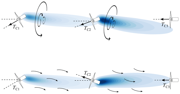
In Fig. 8a, it is observed that C_P,C1 remains relatively constant until γ₁ is changed, indicating that the upwind turbines are not affected by the operating conditions of the downstream rows. The value of C_P,C1 decays roughly as cos ³(γ₁), as discussed in Sect. 3.1.2. Further downstream, C_P,C2 exhibits a dual dependence on γ₁ and γ₂. For a given γ₁, C_P,C2 changes as a cosine function of γ₂, and the maximum achievable C_P,C2 increases with larger γ₁. Interestingly, the γ₂ value corresponding to each local maximum of C_P,C2 is also dependent on γ₁: it has the opposite sign, and its magnitude grows as |γ₁| increases. Therefore, for a given γ₁, the cumulative power of C1 and C2 is maximized not by aligning the downstream turbine with the incoming wind direction, as intuition might suggest, but by yawing it in the opposite direction of the upstream turbine. This behaviour, which is also observed in the lateral columns, is in agreement with the findings of McKay et al. (2013) and of Bartl et al. (2018) for turbines operating in partial wakes. It also prompted the inclusion of configurations with γ₃≠0° in EXP2. The most likely explanation is that the sidewash that accompanies the CVPs behind the first row of turbines induces a significant reorientation of flow upstream of the second row. As a result, when the turbines in the second row are yawed in the opposite direction as the ones in the first, they are effectively realigned with the local wind. This is illustrated in a qualitative sketch in Fig. 9b. Considering that Wang et al. (2018) showed that the region of sidewash extends outside of the wake and that Fleming et al. (2018) observed constructive interactions between wakes and vortices of turbines in the same row, the spanwise velocity component may be further amplified due to the close spacing of the turbine columns in this experiment.

Figure 9 Qualitative representation of the most relevant flow phenomena in the two types of yaw configuration: (a) Type 1, in which both γ₁ and γ₂ are positive; and (b) Type 2, in which γ₁>0° and γ₂<0°.

Furthermore, it is reasonable to hypothesize that the flow downstream of C2, deflected in opposite directions by the first two turbines, closely realigns with the column axis. Additionally, the higher power extraction by C2 corresponds to an increased thrust force T_C2 (see Fig. 6), which intensifies the velocity deficit upstream of C3. These phenomena account for the reduced power production of the turbines in the third row observed in Type 2 configurations, compared to greedy operation. Figure 8 presents an example of such a configuration, highlighted with square symbols, where γ₁=10.8°, ${\mathit{\gamma }}_{\mathrm{2}}=-\mathrm{5.4}\mathit{°}$, and $\mathrm{\Delta }{C}_{\mathrm{P},\mathrm{farm}}=+\mathrm{3.3}\mathit{\%}$. This demonstrates that the farm-power production can be increased by optimizing the collective performance of the first two rows at the expense of the third.

Figure 10 Sum of the C_P of the two downstream turbines in the left (a), central (b) and right column (c). The abscissas identify the configuration number in chronological order, as in Fig. 8. The colour scheme represents the yaw angle of the turbines in the second row. The horizontal dash-dotted lines represent the corresponding values in the greedy configuration.

In Type 1 configurations, where both γ₁ and γ₂ are positive, power production is more evenly distributed across all rows. This can be inferred by considering the sum of the C_P values of the two downstream turbines, illustrated for all columns in Fig. 10. For each γ₁, the cumulative power exhibits a similar trend to that of C_P,C2 seen in Fig. 8b, albeit less pronounced and with greater scatter in certain cases. Unlike C_P,C2, however, local maxima are more frequently observed at γ₂>0°, particularly when γ₁>0° (Config. nr. 56 and above). This is in spite of the fact that, as stated above, the power of the second turbine would be higher if it were yawed in the negative direction while γ₁>0°. Consequently, in these configurations, the wind speed upstream of the third row must be sufficiently high to offset the missed production in the second row. Such elevated velocity likely arises from the interaction between the wake of the second turbine and the CVP, and the consequent sidewash of the first turbine. The resulting amplified deflection of the second wake, induced by the yawed wake of the upstream turbine, may be understood as a generalization of the phenomenon known as secondary steering, described by Fleming et al. (2018).

Additionally, Fig. 10 shows that the sum of the downstream C_P is more sensitive to changes of γ₂ when γ₁>0° ($\mathrm{Config}.\mathrm{nr}.\ge \mathrm{56}$) than when γ₁<0° ($\mathrm{Config}.\mathrm{nr}.<\mathrm{56}$). This effect is particularly noticeable in the lateral columns, but it can also be observed at large magnitudes of γ₁ in the central column. This increased sensitivity suggests that the interactions between the wakes and CVPs of the upstream turbines with those of the second-row rotors are more effective when γ₁>0°. As a result, adjusting γ₂ in these cases can have a greater impact on the velocity deficit upstream of the third row, potentially leading to larger cumulative C_P. Conversely, these interactions are less prominent when γ₁<0°. In these cases, most of the additional power produced by the third-row turbines derives from the energy not extracted by the second-row rotors, and vice versa, leading to smaller variations of the cumulative C_P. Previous studies have found that the sense of rotation of the wake and the presence of the shear layer due to the ABL can result in larger wake deflection in one yaw direction than the other (Fleming et al., 2018; Zong and Porté-Agel, 2020). Additionally, Bastankhah and Porté-Agel (2016) showed that yawed turbine wakes also exhibit a vertical displacement, which can be pointed upwards or downwards depending on the yaw direction. These asymmetries in the deflection of the upstream turbine wakes, relative to the sign of γ₁, are therefore likely to modulate the wake steering of the second-row rotors.

It should be noted that the low design tip-speed ratio and consequent high torque cause the wake swirl of the turbine models used in this study to be more pronounced compared to full-scale turbines operating at λ≥6 (Bourhis et al., 2022). As a result, the effects of wake interactions observed here may be somewhat accentuated. Nevertheless, the observation of similar asymmetries in wind-tunnel studies with turbines operating a higher tip-speed ratios (the model used by Bartl et al. (2018) operated at λ=6) indicates that the trends identified here remain qualitatively relevant for full-scale applications.

Figure 11 Variation of the power coefficients of the turbines in the first (a), second (b), and third row (c), normalized with the corresponding value in the greedy configuration and plotted as a function of γ₁. The size of the symbols is representative of the uncertainty related to the zero alignment of the turbines, here assumed to be a single step of the stepper motors, i.e. 1.8°. The solid lines in panels (a), (b), and (c) represent the functions cos ³γ₁, an arbitrary even function, and a linear least-square fit, respectively. Note that the latter two are only used to assist the visualization.

3.1.2 The asymmetry in the farm response

The yaw direction of the turbines in the first row plays a major role in determining whether the farm power will increase or decrease in response to a wake-steering strategy. As mentioned in Sect. 3.1, the model farm outperforms the greedy configuration only if γ₁>0°. This asymmetry is here investigated, restricting the analysis to the subset of the cases from EXP1 in which ${\mathit{\gamma }}_{\mathrm{2}}={\mathit{\gamma }}_{\mathrm{3}}=\mathrm{0}\mathit{°}$, thus isolating the effect of γ₁. The variation of the power coefficients of the turbines in the first, second, and third row as a function of γ₁ are presented in Fig. 11a, b, and c, respectively. As expected, the C_P values of the turbines in the first row diminish monotonically as |γ₁| increases, closely following the empirical formula $C_{\mathrm{P}}\left(\mathit{\gamma }\right)=C_{\mathrm{P}}(\mathit{\gamma }=\mathrm{0}\mathit{°}){\cos }^{\mathrm{3}}\left(\mathit{\gamma }\right)$ found for example in Burton et al. (2011). A small asymmetry is already observable in the lateral columns. In fact, the power of the turbine in the left column decays more slowly (and the one in the right more rapidly) than what is predicted by the cosine relation for γ₁>0°. The opposite is true for γ₁<0°. As the turbines in the first row are yawed farther away from the wind direction, the power produced by the second row increases steadily and can even double as γ₁ approaches ±30°, as observed in Fig. 11b. It can also be noted that the C_P of the turbines in the central and right columns increase faster when γ₁>0°. The turbine on the left column, meanwhile, exhibits a more symmetrical behaviour, except at large values of |γ₁|, where L2 performs better when γ₁<0°. The highest degree of asymmetry is observed in the third row. As seen in Fig. 11c, the power coefficients increase almost linearly as γ₁ transitions from negative to positive values. Furthermore, yawing the first row to a negative angle generally leads to a performance loss in the third-row turbines. Thus, the asymmetry in the farm response is partially attributable to the dependence of the third-row performance on the sign of γ₁.

The asymmetry in the second row likely stems from the aforementioned difference in deflection magnitude for a given |γ₁|, which favours positive yaw angles. It should be noted that the preferred direction of yaw identified in the present experiment, i.e. counterclockwise when seen from the top, is in agreement with the findings of Bartl et al. (2018), whose turbines also rotated counterclockwise when seen from the front. The reverse trend observed for turbine L2 may be due to the fact that a negative γ₁ entails that the wake of turbine L1 is deflected away from the farm, rather than towards it, potentially offsetting the greater deflection observed for positive γ₁.

However, the change in deflection magnitude does not account for the third-row performance exhibiting both improvements and degradations. A more plausible explanation lies in the vertical displacement of the yawed wakes. When Bossuyt et al. (2021) compared the wakes of yaw and tilt-controlled turbines in wind-tunnel experiments, they observed that the downward displacement induced by a negative tilt increases the available power at a downstream turbine by augmenting the downward transfer of kinetic energy. On the contrary, an upward deflection reduces the velocity impinging on the upper section of the downstream rotor. Considering that yaw misalignment can also induce a minor vertical deflection and that Bastankhah and Porté-Agel (2016) observed a downward displacement for positive yaw angles (adjusted for the different sign convention used in this work), this mechanism may provide a more comprehensive explanation for the bidirectional impact of γ₁ on the third-row turbines. It is worth recalling that the turbine model employed by Bastankhah and Porté-Agel (2016) served as the basis for rotor geometry used in this work.

3.1.3 Difference between columns

The previous discussion highlighted the fact that turbines in the same row have different responses to a given yaw configuration. In fact, the performance of each column is also affected differently. This is illustrated in Fig. 12, which displays the change of column-power coefficient C_P,col, defined as the average C_P of the turbines in a given column, for all the configurations tested in EXP1 and EXP2. Here, the values of ΔC_P,col are plotted against the ΔC_P,farm of the respective configuration. The farm-optimal case, i.e. $\stackrel{\mathrm{‾}}{\mathit{\gamma }}=\left(\mathrm{18}\mathit{°},\mathrm{10.8}\mathit{°},\mathrm{0}\mathit{°}\right)$, is thus found at the right end of the figure. Interestingly, while this configuration also maximizes the C_P,col of the left and centre columns, the right column is optimized at a different configuration, namely $\stackrel{\mathrm{‾}}{\mathit{\gamma }}=\left(\mathrm{18}\mathit{°},\mathrm{14.4}\mathit{°},-\mathrm{5.4}\mathit{°}\right)$. The improvements of left, centre, and right columns in the farm-optimal case are 5.8 %, 4 %, and 6.1 %, respectively. This grows to 6.9 % for the right column in its optimal case. Figure 12 also indicates that the farm-power improvements are limited by the response of the central column, which is generally weaker than that of the lateral ones. The central column is also the one exhibiting the lowest C_P,col in greedy operation, primarily because of the low performance of turbine C2, as will be further discussed in Sect. 3.3. The diminished response of the central column to wake-steering control may be further examined by considering how the power is distributed in the columns. On average across the 15 best cases (relative to the farm power), the two downwind turbines account for 52.9 % of the total production in the left column and 53.6 % in the right one. In the central column, the share drops to 48.7 %. As a reference, the six downwind turbines contribute to 42.7 % of the farm power in greedy operation. This difference suggests that the additional kinetic energy available to the downstream turbines, following yaw actuation, is more significant in the lateral columns than in the central one. This may be partly attributed to the higher velocity measured at the edges of the test section prior to farm installation (see Fig. 3b) and partly to the close spacing of the columns, which may restrict the entrainment of kinetic energy into the centre of the array compared to its sides.

Figure 12 Change of the power coefficients of the three columns, relative to the respective greedy values, versus the change in farm-power coefficient of the corresponding configuration. The solid lines indicate moving averages, whereas the diamond and pentagram symbols denote the farm-optimal and column-optimal cases, respectively. The inset provides a close-up of the best-performing configurations.

3.1.4 Influence of the side walls

The asymmetry in farm response and the differences between the columns discussed in the previous sections may also seem attributable to another important feature of the current experimental setup: the presence of the wind-tunnel sidewalls. However, while the small separation between the lateral columns and the walls may allow the wakes of the former to interact with the boundary layers developing over the latter, such interaction is unlikely to qualitatively affect the farm response. In fact, if wake-wall coupling were a dominant flow feature, the performance of the lateral columns would likely be maximized either when the wakes of the first-row turbines are deflected away from the walls (γ₁>0° for the left column and γ₁<0° for the right one) or when the wakes are deflected towards the walls (γ₁<0° for the left column and γ₁>0° for the right one). Instead, both columns achieve the highest efficiencies when γ₁>0°, indicating that there must be another primary mechanism determining the farm asymmetry with respect to the sign of γ₁ and the behaviour of the lateral columns. Furthermore, if the walls acted as a constraint to the wake deflections, the lateral column whose wakes are steered towards the walls would be expected to exhibit a lower ΔC_P,col than the other two columns. However, this is not observed. Instead, in most of the farm-optimal configurations, which feature γ₁>0° and γ₂>0°, the right column experiences higher gains that the left one, as shown on the right side of Fig. 12. Therefore, the primary effect of the tunnel walls is likely to be an amplification the flow acceleration at the sides of the farm.

3.1.5 Yawing the third row

As discussed in Sect. 3.1, the farm power can be increased by yawing the trailing-row turbines. To illustrate this effect, Fig. 13 presents the C_P variation of the turbines in the central column, measured in EXP2. The turbine performance displays the same characteristics outlined in Sect. 3.1.1, namely the cosinusoidal decay of C_P,C1 and the dual dependence of C_P,C2 on γ₁ and γ₂. In addition, Fig. 13c shows that C_P,C3 is only marginally affected by γ₃ at small values of γ₁. However, a distinct trend emerges on the right-hand side of the figure, where γ₁ is large: with constant γ₁ and γ₂, turbine C3 is less productive at ${\mathit{\gamma }}_{\mathrm{3}}=+\mathrm{5.4}\mathit{°}$ than at γ₃=0°, and it is often more efficient at ${\mathit{\gamma }}_{\mathrm{3}}=-\mathrm{5.4}\mathit{°}$, i.e. when it is yawed in the opposite direction of the turbines upstream. This trend is further highlighted in Fig. 13d and mirrors the behaviour observed (in both experiments) for the second-row turbines, albeit with a reduced impact on the power coefficient. The same pattern is observed in the lateral columns.

Figure 13 C_P of the central turbines C1 (a), C2 (b), and C3 (c). The abscissa identifies the configuration number, following the chronological order in which the configurations were tested. The colour scheme represents the value of γ of the corresponding turbine. The horizontal dash-dotted lines indicate the C_P value in the greedy configuration, while the diamond symbol denotes the farm-optimal configuration. (d) Magnified view of C_P,C3 in the two last subgroups of configurations, in which γ₁=18° and γ₁=21.6°.

3.2 Thrust force

The turbine towers in the central columns were also equipped with strain gauges, measuring the axial component of the thrust force T. The thrust coefficients measured during EXP2 are presented in Fig. 14. Notably, the behaviour of C_T displays the same features as that of C_P: C_T,C1 is independent of the downstream conditions and decays as a cosine function of γ₁, while C_T,C2 is largest for a given γ₁ when C2 is yawed in the opposite direction. This further corroborates the hypothesis that, in Type 2 configurations, the wake deficit downstream of the second turbine is large, leading to a reduced production in the third row. Additionally, the data are consistent with the findings of Bartl et al. (2018), who further reported a reduction in the yaw moments on the second turbine in this type of configuration.

Figure 14 Thrust coefficient of turbines C1 (a), C2 (b), and C3 (c), measured during EXP2. The horizontal axis identifies the configuration number, following the chronological order in which the configurations were tested. The colour scheme represents the value of γ of the corresponding turbine. The horizontal dash-dotted lines indicate the thrust in the greedy configuration, while the diamond symbol denotes the farm-optimal configuration.

Figure 15 Thrust coefficient of turbines C1 (a), C2 (b), and C3 (c) versus the change in farm-power coefficient. The data from both EXP1 and EXP2 are included. The colour scheme represents the value of γ of the corresponding turbine. The horizontal dash-dotted lines indicate the T value in the greedy configuration, while the diamonds denote the farm-optimal case.

Figure 16 Standard deviation of the thrust coefficient time signals versus the change in farm-power coefficient. The data correspond to turbine C1 (a), C2 (b), and C3 (c). Both EXP1 and EXP2 are included. The colour scheme represents the value of γ of the corresponding turbine. The horizontal dash-dotted lines indicate the σ_T value in the greedy configuration, while the diamonds denote the farm-optimal case.

Furthermore, Figs. 15 and 16 display the impact of wake-steering control on the C_T and its fluctuations, respectively, highlighting how these quantities change with increasing farm power. In most of the best-performing configurations, C_T,C1 decreases while ${\mathit{\sigma }}_{C_{\mathrm{T}},\mathrm{C}\mathrm{1}}$ increases compared to the greedy case. There are however several instances in which both quantities are lower while the farm power is higher than the baseline, indicating the possibility of a multi-objective optimization aimed at maximizing the power while minimizing the fatigue loads. In the case of turbine C2, the thrust coefficient and its standard deviation exhibit significant variations but remain only moderately higher than the greedy value in the optimal cases. In contrast, both C_T,C3 and ${\mathit{\sigma }}_{C_{\mathrm{T}},\mathrm{C}\mathrm{3}}$ increase steadily with improving farm performance. Turbine C3 is also the one with the largest baseline fluctuation magnitude, which is expected as the turbulence intensity is known to increase further into the array. Relative to the mean C_T, the fluctuations grow progressively from one row to the next.

3.3 Effect of free-stream velocity

In order to investigate the influence of the free-stream velocity on the efficacy of wake-steering control, two additional experiments were performed, with U_∞=8 and 9 m s⁻¹. The corresponding U_hub are 6.8 and 7.65 m s⁻¹, respectively. Lower values of U_∞ were excluded from this study since the downstream turbines would experience velocities below the cut-in threshold in multiple configurations, including the greedy case. This would cause those rotors to cease rotation, thereby invalidating the comparison with higher U_∞. As summarized in Table 4, the configurations evaluated here are the subset of those from EXP2 where γ₃=0°, with the inclusion of one more possible value for γ₁, namely 25.2°. The values of ΔC_P,farm measured with the three velocities are compared in Fig. 17. The results indicate that the maximum power gain decreases with increasing U_∞. In fact, ΔC_P,farm falls from 5.3 % at 7 m s⁻¹ to 1.9 % and 1.3 % at 8 and 9 m s⁻¹, respectively.

Table 4 Ranges and resolutions of the yaw angles considered for each row of turbines in the experiment investigating the effect of the free-stream velocity. Each interval is defined as initial angle: step angle: final angle.

Figure 17 Normalized change of farm-power coefficient as a function of the yaw angles of the first-row turbines (abscissa) and second-row turbines (ordinate). The three panels correspond to different free-stream velocities: (a) U_∞=7 m s⁻¹, (b) U_∞=8 m s⁻¹, and (c) U_∞=9 m s⁻¹.

A similar trend can be observed considering the changes in C_P,col, shown in Fig. 18a, with the exception of the left column, which experiences a larger improvement at 9 m s⁻¹ than at 8 m s⁻¹. Interestingly, the central column exhibits higher improvements than the other two at 8 m s⁻¹ but performs the worst at the other speeds. This behaviour may be attributed to local flow accelerations induced by the wind-tunnel characteristics and the devices used to replicate the ABL. These could result in deviations from the horizontal velocity profile presented in Fig. 3. The reduction in power gains can be partly explained by the fact that the farm C_P,gr, used as a reference, increases from 0.178 at 7 m s⁻¹ to 0.192 at 8 m s⁻¹ and to 0.198 at 9 m s⁻¹. Thus, the array in greedy conditions becomes more efficient with increasing free-stream velocity, which may limit the scope for improvement through control strategies. Moreover, the additional power is not uniformly distributed within the model farm: as seen in Fig. 18b–d, the largest performance growth takes place in the first row of turbines, whose C_P,gr increases on average by 14.5 % from U_∞=7 m s⁻¹ to U_∞=9 m s⁻¹. The baseline production of the second and third rows is only enhanced by 7.6 % (most of which is due to the power change of C2) and 6.1 %, respectively. This indicates that only a small amount of the additional kinetic energy available in the free stream is entrained deep into the array and can reach the downstream turbines. The change in C_P of the first row is likely caused by a Reynolds-number dependence of the turbine power characteristics. It is also possible that the ratio between U_∞ and U_hub may not be constant, as initially assumed, which would inflate (or deflate) the estimated undisturbed U_hub and thus the C_P. However, this would apply equally to the whole array and therefore does not explain the differences between rows. Even though the fraction of total power generated in the upstream row increases only modestly, from 57.3 % at U_∞=7 m s⁻¹ to 59 % at U_∞=9 m s⁻¹, it is sufficient to make it less advantageous to sacrifice the performance of those turbines to benefit the ones downstream. Consequently, the best-performing configurations at higher U_∞ are characterized by smaller values of γ₁, as shown in Fig. 18e–g, which makes them more similar to the greedy one. As a result, the maximum power increment among these cases is diminished. This is analogous to what is observed at U_∞=7 m s⁻¹ for the central column. As illustrated in Fig. 18c, the C_P of turbine C2 is lower than that of L2 or R2. Consequently, it is less advantageous to forgo the production of turbine C1 to benefit C2, resulting in a smaller mean γ₁ in the best configurations for the central column compared to the others, as depicted in Fig. 18e.

Figure 18 Maximum normalized change of power coefficient for the three columns and for the entire farm at the three free-stream velocities (a). Greedy power coefficients of the turbines in the first row (b), second row (c), and third row (d). Yaw angles of the turbines in the first two rows averaged among the 15 best cases relative to each column, with U_∞=7 m s⁻¹ (e), U_∞=8 m s⁻¹ (f), and U_∞=9 m s⁻¹ (g). The angle of the third row is not represented as γ₃=0° in all cases.

An additional remark can be made about the optimal angles of the second row. As stated in Sect. 3.1, the optimal configurations are characterized by values of γ₂ that are smaller or, in some cases, equal to γ₁. Figure 18e–g reveal that the average γ₂ among the best cases decreases significantly from U_∞=7 to 8 m s⁻¹. However, at U_∞=9 m s⁻¹, the optimal γ₂ of the lateral columns are once again large and comparable to the corresponding γ₁. This observation is consistent with the fact that the C_P,col of the left column improves more at U_∞=9 m s⁻¹ than at 8 m s⁻¹, and it points to the non-linear influence exerted by the free-stream velocity on the energy trade-offs taking place within the farm. Furthermore, the large values of γ₁ and γ₂ in the best configurations indicate that the lateral columns would probably experience an additional, non-negligible power gain from yawing the third row.

3.4 A note on the choice of degrees of freedom

Since each column responds differently to a given yaw configuration, as discussed in Sect. 3.1.1, it is natural to wonder whether it is possible to achieve further power improvements by controlling each column independently, thus extending the number of degrees of freedom from 3 to 9. To assess this hypothesis, in one last experiment the model farm was tested while yawing each column to one of the configurations that gave the best improvements of its respective C_P,col. The 150 cases examined here come from all the possible combinations of the six best configurations for the left column and the five for the centre and right columns. These were chosen from EXP1 and EXP2, as well as some additional experiments that have not been presented in this work for the sake of brevity and because they do not provide further insights. The results indicate that the model farm does not experience further power gains compared to the configurations in which all the turbines in a row were yawed equally. The maximum improvement measured here was $\mathrm{\Delta }{C}_{\mathrm{P},\mathrm{farm}}=\mathrm{4.8}\mathit{\%}$, which corresponds to the configuration with $\stackrel{\mathrm{‾}}{{\mathit{\gamma }}_{\mathrm{L}}}=\left(\mathrm{19.8}\mathit{°},\mathrm{14.4}\mathit{°},-\mathrm{3.6}\mathit{°}\right)$, $\stackrel{\mathrm{‾}}{{\mathit{\gamma }}_{\mathrm{C}}}=\left(\mathrm{18}\mathit{°},\mathrm{3.6}\mathit{°},\mathrm{0}\mathit{°}\right)$, and $\stackrel{\mathrm{‾}}{{\mathit{\gamma }}_{\mathrm{R}}}=(\mathrm{18}\mathit{°},\mathrm{16.2}\mathit{°},-\mathrm{7.2}\mathit{°}$ for the left, centre, and right column, respectively). The range of yaw angles from the configurations tested in this experiment is too limited to draw comprehensive conclusions regarding the mutual influences that each column exerts on the others. Nonetheless, it was sufficient to observe that the right column tends to perform slightly better when the yaw angle of turbine L1 is large. This suggests that it may be worth conducting a parametric study on such influences, as they are likely to play a key role in wake-steering control of farms with close spanwise spacings between columns.

4 Comparison with results from the literature

The largest overall power gain reported in this work, +5.3 %, is considerably lower than some results found in the literature. Considering the differences between those experiments and ours may highlight some key aspects to consider when implementing wake-steering control.

The main difference between this work and that of Campagnolo et al. (2016) is that their three turbines were not positioned in an aligned column. Instead, each downstream rotor was offset by 0.5 D in the spanwise direction relative to the one directly upstream. This meant that, for sufficiently large yaw angles of the first two turbines, the interaction of their wakes with the downstream turbines could almost entirely be removed, leading to larger power increments (up to 15 %).

The comparison with the results of Bastankhah and Porté-Agel (2019) is of particular interest, given that the turbine geometries are very similar (see Sect. 2.2), while the turbine diameter and streamwise spacing are identical. Additionally, both experimental setups present an ABL inflow with comparable ${\mathit{\delta }}_{\mathrm{99}}/D$. The primary distinctions are that the hub velocity in their work is lower (4.8 m s⁻¹ vs 5.95 m s⁻¹), as are their friction velocity u^* and roughness length z₀, and that their array consists of a single column. When considering only the first three of their five turbines, Bastankhah and Porté-Agel (2019) achieved a power gain of 8 %, with the first two turbines yawed by approximately 25 and 15°, respectively. In our experiments, only the lateral columns come close to such improvements, with the left column improving by up to 5.8 % and the right one by up to 6.9 %, as reported in Sect. 3.1.3. These shortcomings may be explained by the higher U_hub used here, in accordance with the discussion in Sect. 3.3. The stark discrepancy between our central column, which improves by only 4 %, and the results of Bastankhah and Porté-Agel (2019) further emphasizes the impact of the close spacing between columns on the efficacy of wake-steering control.

The study conducted by Rotea et al. (2024) offers a valuable comparison of the usefulness of yaw-control strategies applied to different multi-column wind farm models. The power gain that they reported is about 9 %, and there are several differences between their experiment and ours that are worth examining. While both turbine geometries are based on the model proposed by Bastankhah and Porté-Agel (2017), their rotor has a larger diameter (0.2 vs 0.15 m). Both the mean velocity and the turbulence intensity at hub height are higher in the setup of Rotea et al. (2024), which, according to our discussion in Sect. 3.3 and the findings of Bartl et al. (2018), should reduce the control efficacy. However, the spanwise distance between columns is larger in their case (4 D vs 2.67D), and the additional turbine row is expected, based on the results of Bastankhah and Porté-Agel (2019), to enable additional performance improvements. An additional point of divergence, whose impact on wake steering is unknown, is the shear exponent of the ABL inflow α, which is higher in their case: 0.2 vs 0.14. Their exponent is typically associated with rougher terrains and woodland areas (Counihan, 1975). It is important to note that Rotea et al. (2024) restricted their control actuation to two of the four rows – either the first and second or the first and third. Without this constraint, they might have measured even higher gains. Finally, another reason behind their greater improvements is that the power losses of their turbines in the first row, which are yawed by nearly 30°, are only about 20 %. In comparison, Fig. 11a illustrates that our first-row turbines, when yawed by similar angles, lose up to 30 % of their power. Clearly, the increased sensitivity to yaw exhibited by our rotors affects the energy trade-offs between the turbine rows, limiting the potential power gains.

5 Conclusions

In this work, the impact of wake-steering control has been systematically tested by monitoring the performance of a model wind farm operating in a large number of yaw configurations. The largest measured power improvement was about +5.3 %, achieved with the angles $\stackrel{\mathrm{‾}}{\mathit{\gamma }}=\left(\mathrm{18}\mathit{°},\mathrm{10.8}\mathit{°},\mathrm{0}\mathit{°}\right)$. The response of the farm is asymmetric with respect to the direction of the yaw angle of the turbines in the first row, with only positive angles (counterclockwise when seen from an upstream perspective) leading to power gains. It is speculated that this is caused by the interaction of the wake rotation with the counter-rotating vortex pair that forms in yawed wakes. This interaction influences the magnitude of the lateral deflection and determines the direction of the vertical wake displacement, which may play a role in the energy trade-offs that make wake-steering control strategies beneficial.

Considering the C_P of the individual turbines in one column, it is found that the power produced by the turbines in the second row is maximized when they are yawed in the opposite direction of the upstream rotors, i.e. a negative yaw. This leads to the identification of two types of configuration: Type 1, where the first two rows are both yawed by positive angles and the power production is distributed more evenly throughout the farm; and Type 2, in which the power is concentrated in the first two rows, maximizing the production of the turbines in the second row at the expense of the ones in the last row. It is found that, in general, Type 1 configurations lead to better results, with the maximum power increment recorded in a Type 2 configuration being +3.3 % compared to the +5.3 % in Type 1.

It is observed that the three columns of turbines respond differently to the same configuration and in particular that the lateral columns experience the largest improvements from wake steering. A possible explanation is that, for the lateral column, kinetic energy may be entrained both from above and from the edges of the array, whereas in the case of the central column this may be limited to the upper part of the wakes. Additionally, it is found that finely tuned configurations, in which each row is yawed independently from the others according to the configurations that lead to the respective best results, do not yield additional power extraction. This is likely due to the non-linear interaction between the columns and the incoming boundary-layer flow.

In addition, it is reported that the benefits of wake steering tend to diminish with increasing free-stream velocity. This is partly caused by the increased efficiency measured at higher speeds in the greedy configuration and partly the fact that this improved performance is not uniformly distributed within the farm but is concentrated in the turbines in the first row. The resulting change in the energy trade-offs makes it less advantageous to yaw the first-row turbines by large angles and therefore limits the possible improvements to the farm power.

Finally, it is worth noting that the power improvements recorded in this work are lower than other examples found in the literature. This may be caused by a multitude of parameters concerning the experimental setups. One such parameter is the hub velocity, as demonstrated in this article. Other examples may include the turbine size, the C_P,max and operating tip-speed ratio, the farm geometry, and the properties of the ABL in the rotor-swept area, to name but a few. Further investigations are therefore needed in order to determine which of these factors are more important in determining the maximum possible power improvements.