Power output of turbines mounted on tension-leg platforms subjected to fully developed ocean gravity waves

A concern in the deployment of large wind turbines on ocean floating platforms is the effect of floating-platform motions on their electrical power generation. Further, it is not clear how floating motions influence waking, which might affect the combined power generation of collections of turbines. We examine the average power output of a single and a collection of NREL 5 MW wind turbines mounted on a tension-leg platform (TLP) under the action of fully developed ocean wave motions, coupling floating motions with the large-eddy simulation (LES) of atmospheric and rotor dynamics. The ocean dynamics enter as fully developed waves derived from the Pierson–Moskowitz spectrum. To assess the influence of ocean motions, we performed simulations over the full range of wind speeds in the operational range of the turbine, reporting comparisons of average power output when the platforms are allowed to move to when they are held rigidly in place. In all simulations, we find that the effects of the TLP floating-platform's induced motions have a minor effect on single and multiple turbine power production and wake deficits. Even when using coherent and large amplitude harmonic-floating-induced perturbations, any significant wake modifications from floating motions are confined to the near-wake region, where downstream turbines are unlikely to be located. The relatively small amplitude of TLP motions relative to pre-existing turbulent fluctuations are the primary reason for low wake and power modifications downstream.

1 Introduction

The aim of this study is to determine whether, on average, ocean gravity waves affect the average power output of turbines mounted on floating platforms. We do so by comparing the power output of a turbine mounted on a platform allowed to be mechanically affected by wave motions to the same arrangement with no wave motions. We also compare the average power of a simple multi-turbine farm configuration of floating-platform turbines to a fixed-platform arrangement.

The comparison is made via simulations. For the moving platform, we employ large-eddy simulations (LESs) of a stably- and unstably-stratified atmosphere, a mechanical model for the platform, a parametric representation of a 5 MW turbine, and a spectral representation of the ocean gravity waves. The waves and platform dynamics are suppressed when we compute the fixed-platform outcomes. The novelty of the results derives from the complexity of the fully coupled model and the high spatio-temporal resolutions of the simulations.

The simulation of wind turbines has proven to be an effective way to inform the design, siting, and prediction of wind turbine power production (e.g., Wu and Porté-Agel, 2015; Miller et al., 2013). Significant fidelity has been achieved in simulations of individual and clusters of turbines as well as the interaction of turbine wakes and its environment. Offshore sites for wind farms, particularly deep-water ones, have obvious attractive features, among these are lower interference with maritime operations, potentially smaller ecological impact, the possibility of employing larger turbines, and more reliable wind conditions than shallower sites. One obvious challenge to wind turbine deep-water deployment is that they may require a floating platform.

The modeling of floating-platform offshore wind turbines is a multi-scale, multi-physics problem (Lemmer et al., 2018) which can be addressed using varying levels of simulation fidelity. For instance, the work of Wang et al. (2022) used the low-fidelity OpenFAST model with empirical modifications to the drag forces to simulate the wave loads of semi-submersible platforms. While this method improves on the under-predictions of the low-frequency, nonlinear responses from typical engineering models, it does rely on calibration to experimental data. However, the highest-fidelity, blade-resolved simulations including the turbine and floating platform require less empirical calibration but must include boundary layer physics at very small scales. Meanwhile, the regional characterization of the wind resource requires the encapsulation of hour- and kilometer-scale phenomena in mesoscale simulations (i.e., simulations that bridge the scales between highly resolved models and earth system simulations).

The complexity and multitude of design considerations associated with the various platform configurations has shown the need for comprehensive studies on the modeling offshore wind platforms and their interactions with the environment. The Offshore Code Comparison Collaboration, Continued with Correlation and Uncertainty Project (OC6) addresses the need for model validation and comparison. Of particular interest to the current work are Phase III (Bergua et al., 2023; Cioni et al., 2023) and Phase IV (Bergua et al., 2024) of the OC6 project, which studied the aerodynamic rotor behavior and full-system, aerodynamic and hydrodynamic interactions of floating platforms. Their results have shown that two-phase flow simulations of semi-submersible and TetraSpar floating platforms (Darling et al., 2025) are able to be successfully compared against experiments, but there are many remaining challenges in these high-fidelity simulations and simplified models of their behavior are still necessary in many instances. Our long-term goal is to create more accurate representations of wind farms in the mesoscale simulations. For this purpose, we argue that LESs are appropriate to resolve atmospheric interactions with turbines, and the momentum and energetic exchanges critical to power generation by the turbines and their effect on the atmospheric boundary layer. LES has been used to compare the effect of moving platform turbine wakes to those of a fixed platform. For example, Johlas et al. (2019, 2020) found that the wakes of these two configurations were similar.

Large-scale simulations using LESs of wind farms are now possible with modern computing tools (Cheung et al., 2022). These studies allow for computation at different atmospheric conditions and are often able to connect to experimental data (Kumer et al., 2016). Unlike blade-resolved models where individual turbines are largely represented in their geometric entirety (see Ribeiro et al., 2023), LES models often represent the turbine via either an actuator line or an actuator disk model (Martinez et al., 2012). The choice of the wind turbine rotor model in high-fidelity wind farm simulations is dependent on both the computational resources available and the expected wake dynamics to be encountered. For instance, in floating turbines with a surge motion frequency commiserate with the rotor speed, a vortex ring state can be encountered if the blade tips interact with the vortex emerging from the previous blade (Sebastian and Lackner, 2011; Kyle et al., 2020) and consequently change the near-field wake. In other cases, an asymmetric loaded rotor (Abraham and Leweke, 2023) or individual pitch control (Cheung et al., 2024) can lead to different loading on individual blades and change the downstream wake behavior. For these situations, an actuator line method or a blade-resolved method may be appropriate to resolve the tip vortex behavior or blade loading differences. However, differences in wake behavior can also be caused by changes to the turbine orientations or to rotor behavior which are not depending on resolving the individual blade loading profiles or tip vortices.

The inclusion of platform motion in the dynamics of turbines has become more prevalent in the literature recently (e.g., Li et al., 2024; Wena et al., 2018; Yang et al., 2022). For instance, wake deflections due to turbine yaw steering (Frederik et al., 2025; Brown et al., 2025) or platform yaw or pitch are a steady phenomenon which can directly impact wind farm performance. Previous studies by Li et al. (2022) and Messmer et al. (2025) have also shown that lower-frequency floating-platform motions can introduce large-scale structures in the far wake which can enhance wake recovery. These effects can be captured using simpler actuator disk models without the need for resolving blade motions or blade pitch controllers, and are the focus of the current study (Dong et al., 2022; Malecha and Dsouza, 2023; Mirocha et al., 2014; Hsieh et al., 2025). The wind tunnel experiments in Wei and Dabiri (2022) report decreased mean power at high tip-speed ratios and high surge due to the stall onset on blades. They were also able to obtain an increase in power under certain controlled wave conditions. Their work points to the importance of having active and passive wave motion control on these floating offshore wind turbines (FOWTs). A significant effort is being made to model and simulate turbine dynamics on moving platforms. These model and simulation efforts are aimed at discerning first-order dynamic/structural issues that will inform the design and construction of these FOWTs. For example, Johlas et al. (2020) compare wake characteristics of turbines mounted on different floating platforms and their wakes to those of fixed turbines.

Here we assess the effect of fully developed ocean gravity waves on the average power output from turbines mounted on a floating platform over a wide range of wind speeds. We focus on the power characteristics of a 5 MW NREL turbine mounted on a specific and familiar moored platform, namely the tension-leg platform. These platforms will have active motion control. We omit active motion control, since active platform stability mechanisms primarily address transient motions due to storms, swells, and developing ocean conditions, and the residual flow due to waves (for example, see McWilliams and Restrepo, 1999; McWilliams et al., 2004; Restrepo, 2007).

Our approach allows us to understand how floating-platform motions from ocean dynamics and turbulent thrust intermittency alters key elements of the flow used in mesoscale parameterizations including hub-height wind speeds and directions, turbulence, and turbine power output over the timescales present in a mesoscale simulation. First, we extend LESs to include floating turbine dynamics such that power production and subsequently turbulent kinetic energy (i.e., the quantities of interest in a mesoscale parameterization) are directly modified by the turbine motions. To do this, we have modified an existing LES tool capable of modeling a variety of atmospheric conditions using an actuator disk approach. The resolution of atmospheric dynamics of these simulations is 10 m. Second, we include explicitly how platform motions affect the wind flow encountering the turbine as well as the effects of platform motion on the mechanics to turbine. Third, we account for how gravity wave motions affect the dynamics of the platform itself.

An ocean platform would be exposed to a variety of different waves. Our study will focus on motions induced by “fully developed” ocean wave conditions. Well-established and verified empirical models for these ocean waves have been around for more than half a century. The most widely cited and tested models for these waves are the Pierson–Moskowitz model (see Pierson and Moskowitz, 1964) and its variant applicable to developing conditions, the more prominently peaked JONSWAP spectrum model (see Hasselmann et al., 1973). The Pierson–Moskowitz model has as input the wind speed at a set reference height above the mean sea elevation, and it produces a multi-spectral description of the gravity wave field, presuming the sea state has reached statistically stationary conditions (fully developed) over sufficiently large expanses (fetches). The gravity waves are, by some measures, the overwhelmingly most common waves found in deep waters, where most of the turbines on floating platforms operate or plan to operate. In the ensemble, these gravity waves are stationary and can be described as having random phases. As a consequence of this choice of the types of waves under consideration, we then exclude swells generated by distant storms and disturbances which manifest themselves as episodic/transient changes in the sea surface, dissipative white-capping waves (typified by random breaking events), or steep episodic breaking waves of large amplitude that result from interactions of the wave field with the underlying ocean currents. Notwithstanding the prevalence of wind waves in places where these floating-platform ocean turbines are placed or are planned for, in the interpretation of the results that follow, it is cautioned that fully developed sea states are not common in nature and thus the Pierson–Moskowitz spectral model for these waves apply with caveats to the practical case. However, the effect on turbine power output due to waves modeled by Pierson–Moskowitz is not at all obvious and a motivation for this paper. Different geographic and weather conditions determine what types of transient oceanic disturbance are prevalent, and thus answering whether waves of this type have an impact on power output of these floating installations will require specifics of geography, time expanse, and large-scale atmospheric conditions to be meaningful.

The remainder of the document is organized as follows. In Sect. 2, we detail the model of the platform/turbine dynamics, responding to wind wave motions. In Sect. 3, we give the problem statement and make plain how the wind exposed to the turbines is affected by motions of the platform. In Sect. 4, we provide details on how the turbine is handled numerically and how the atmospheric initial conditions and boundary conditions are chosen for the LES formulation. The LES equations and numerical details appear in Appendix B. In Sect. 5, we describe the results of our numerical experiments. Wherever possible we show relative quantities, comparing power output, for example, of the turbine mounted on a moving platform and the same where the platform is not subjected to ocean waves. Concluding remarks and suggestions for immediate research follow-up appear in Sect. 6.

2 Platform dynamics

Our modeling approach for the simulation of the FOWTs dynamics is adapted from Betti et al. (2014). A schematic of the platform and turbine appear in Fig. 1. In what follows, we will be specifically using the parameters associated with an NREL 5 MW turbine, mounted on a floating platform. All of the parameters required to re-create the platform motions we use in this study are found in Betti et al. (2014).

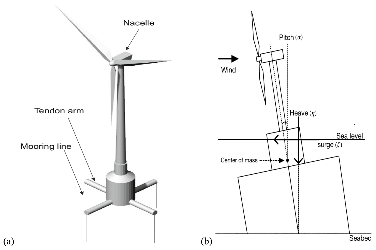
Figure 1 Offshore wind turbine floating platform. The platform is a partially submerged, chain-stabilized design. Panel (a) is reproduced from Karimi et al. (2017). Panel (b) is reproduced from Liu and Chertkov (2023). The turbine parameters correspond to an NREL 5 MW design (Papi and Bianchini, 2022).

Generally, we would have 12 degrees of freedom (DOFs): surge, heave, and pitch position, which are the symmetric motions; and the antisymmetric motions are sway, roll, yaw position (the other 6 DOFs are the velocities of each aforementioned position). In what follows, however, we will always line up the platforms/turbines such that only symmetric degrees need to be considered (see Ribeiro et al., 2023; Fontanella et al., 2025 for studies that focus on the effect of sway surge and yaw effects on turbine wakes). We therefore only consider 6 DOFs: surge ζ, heave η, and pitch α (and their respective velocities), as shown in Fig. 1b. See also Fig. 2 for more details on the coordinates and platform geometry.

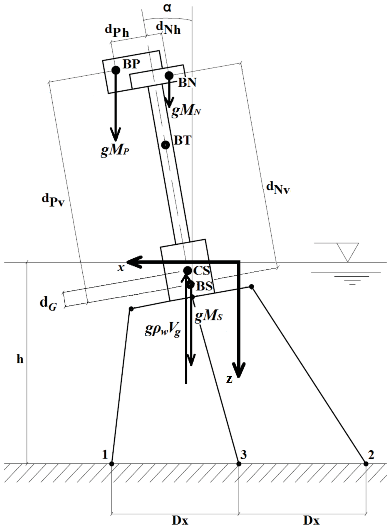
Figure 2 Offshore wind turbine floating platform. Figure reproduced from Betti et al. (2014). BN is the nacelle center of mass, BT is the tower center of mass, BS is the center of mass of float and tower, BP is the center of mass of the fan, CS is the center of thrust of the buoyancy force, and Dx is the attachment point inter-distance.

In this model, the balance of forces and torques for the surge, heave, and pitch are

$$\begin{array}{}\text{(1)}& E\dot{q}=F,\end{array}$$

with the overdot indicating a time, t, derivative. Here, $q=[\mathit{\zeta },\dot{\mathit{\zeta }},\mathit{\eta },\dot{\mathit{\eta }},\mathit{\alpha },\dot{\mathit{\alpha }}{]}^{\top }:=[\mathit{\zeta },u,\mathit{\eta },v,\mathit{\alpha },w{]}^{\top }$; the inertia matrix E is defined as

$$\begin{array}{}\text{(2)}& \mathbf{E}=\left[\begin{array}{cccccc}\mathrm{1}& \mathrm{0}& \mathrm{0}& \mathrm{0}& \mathrm{0}& \mathrm{0}\\ \mathrm{0}& M_X& \mathrm{0}& \mathrm{0}& \mathrm{0}& M_{\mathrm{d}}\cos \mathit{\alpha }\\ \mathrm{0}& \mathrm{0}& \mathrm{1}& \mathrm{0}& \mathrm{0}& \mathrm{0}\\ \mathrm{0}& \mathrm{0}& \mathrm{0}& M_Y& \mathrm{0}& M_{\mathrm{d}}\sin \mathit{\alpha }\\ \mathrm{0}& \mathrm{0}& \mathrm{0}& \mathrm{0}& \mathrm{1}& \mathrm{0}\\ \mathrm{0}& M_{\mathrm{d}}\cos \mathit{\alpha }& \mathrm{0}& M_{\mathrm{d}}\sin \mathit{\alpha }& \mathrm{0}& J\end{array}\right],\end{array}$$

and the forcing vector is

$$\begin{array}{}\text{(3)}& \mathit{F}=\left[\begin{array}{c}u\\ Q_{\mathit{\zeta }}+M_{\mathrm{d}}{w}^{\mathrm{2}}\sin \mathit{\alpha }\\ v\\ Q_{\mathit{\eta }}-M_{\mathrm{d}}{w}^{\mathrm{2}}\cos \mathit{\alpha }\\ w\\ Q_{\mathit{\alpha }}\end{array}\right].\end{array}$$

The weight forces are

$$\begin{array}{}\text{(4)}& {\displaystyle }{Q}_{\mathit{\zeta }}^{\left(\mathrm{we}\right)}=\mathrm{0},\text{(5)}& {\displaystyle }{Q}_{\mathit{\eta }}^{\left(\mathrm{we}\right)}=(M_{\mathrm{N}}+M_{\mathrm{P}}+M_{\mathrm{S}})g,\text{(6)}& {\displaystyle }\begin{array}{rl}{Q}_{\mathit{\alpha }}^{\left(\mathrm{we}\right)}& =\left[(M_{\mathrm{N}}dNv+M_{\mathrm{P}}{d}_{\mathrm{P}v})\sin \mathit{\alpha }\right.\\ & \left.+(M_{\mathrm{N}}dNh+M_{\mathrm{P}}{d}_{\mathrm{P}h})\cos \mathit{\alpha }\right],\end{array}\end{array}$$

where M_N, M_P, and M_S are the masses of the systems N, P, and S shown in Fig. 2. The d_Pv, d_Nv, d_Ph, and d_Nh are the distances between BS and BP, and between BS and BN in the direction parallel to the tower's axis v and horizontal axis h, $d_{\mathrm{N}}=\sqrt{d_{Nh}^{\mathrm{2}}+d_{Nv}^{\mathrm{2}}}$. Buoyancy forces are defined as

$$\begin{array}{}\text{(7)}& {\displaystyle }{Q}_{\mathit{\zeta }}^b& {\displaystyle }=\mathrm{0},\text{(8)}& {\displaystyle }{Q}_{\mathit{\eta }}^b& {\displaystyle }=-\mathit{\rho }w{V}_{g}g,\text{(9)}& {\displaystyle }{Q}_{\mathit{\alpha }}^b& {\displaystyle }=\mathit{\rho }w{V}_g{d}_G\sin \mathit{\alpha },\end{array}$$

and wave forces as

$$\begin{array}{}\text{(10)}& {\displaystyle }{Q}_{\mathit{\zeta }}^{\left(\mathrm{wa}\right)}& {\displaystyle }=(\mathit{\rho }{V}_g+m_x)\cos \mathit{\alpha }\ddot{z},\text{(11)}& {\displaystyle }{Q}_{\mathit{\eta }}^{\left(\mathrm{wa}\right)}& {\displaystyle }=(\mathit{\rho }{V}_g+m_x)\sin \mathit{\alpha }\ddot{z},\text{(12)}& {\displaystyle }{Q}_{\mathit{\alpha }}^{\left(\mathrm{wa}\right)}& {\displaystyle }=\mathrm{0}.\end{array}$$

Wind forces Q^wi are

$$\begin{array}{}\text{(13)}& {\displaystyle }{Q}_{\mathit{\zeta }}^{\left(\mathrm{wi}\right)}=& {\displaystyle }-\left(FA+FAN+FAT\right)\text{(14)}& {\displaystyle }{Q}_{\mathit{\eta }}^{\left(\mathrm{wi}\right)}=& {\displaystyle }\mathrm{0}\text{(15)}& {\displaystyle }{Q}_{\mathit{\alpha }}^{\left(\mathrm{wi}\right)}=& {\displaystyle }-FA\left(d_{\mathrm{P}v}\cos \mathit{\alpha }-d_{\mathrm{P}h}\sin \mathit{\alpha }\right)\text{(16)}& {\displaystyle }& {\displaystyle }-FAN\left(d_{Nv}\cos \mathit{\alpha }-d_{Nh}\sin \mathit{\alpha }\right)\text{(17)}& {\displaystyle }& {\displaystyle }-FAT\left(d_{\mathrm{T}}\cos \mathit{\alpha }\right)\end{array}$$

$$\begin{array}{}\text{(18)}& {\displaystyle }FA=& {\displaystyle \frac{\mathrm{1}}{\mathrm{2}}}\mathit{\rho }A{C}_{\mathrm{T}}{\left(u_{\mathrm{upstream}}+v_{\mathit{\zeta }}+\sqrt{d_{\mathrm{P}h}^{\mathrm{2}}+d_{\mathrm{P}v}^{\mathrm{2}}}w\cos \mathit{\alpha }\right)}^{\mathrm{2}}\text{(19)}& {\displaystyle }FAN=& {\displaystyle \frac{\mathrm{1}}{\mathrm{2}}}\mathit{\rho }{C}_{\mathrm{dN}}{A}_{\mathrm{N}}\cos \mathit{\alpha }{\left(u_{\mathrm{upstream}}+v_{\mathit{\zeta }}+d_{N}w\cos \mathit{\alpha }\right)}^{\mathrm{2}}\text{(20)}& {\displaystyle }FAT=& {\displaystyle \frac{\mathrm{1}}{\mathrm{2}}}\mathit{\rho }{C}_{\mathrm{dT}}{h}_{\mathrm{T}}{D}_{\mathrm{T}}\cos \mathit{\alpha }{\left(u_{\mathrm{upstream}}+v_{\mathit{\zeta }}+d_{\mathrm{T}}w\cos \mathit{\alpha }\right)}^{\mathrm{2}},\end{array}$$

where u_upstream is the freestream inflow velocity to the turbine actuator disk described in Eq. (22) and provided by the LES model, A is the turbine-swept plan area, C_T is the coefficient of thrust, C_dN=1 is the coefficient of drag for the nacelle, A_N=9.62 m² is the nacelle area, C_dT=1 is the coefficient of drag for the tower, h_T=87.6 m is the exposed tower height, D_T=4.935 m is the mean tower diameter, and d_T=75.7843 m is the vertical distance between BS and BT in Fig. 2.

We refer the reader to Betti et al. (2014) for the definition of tie rod forces Q^tr and hydraulic drag forces Q^hy. The composite forces are then

$$\begin{array}{}\text{(21)}& \begin{array}{rl}{Q}_{\mathit{\zeta }}& =Q_{\mathit{\zeta }}^{\left(\mathrm{we}\right)}+Q_{\mathit{\zeta }}^{\left(b\right)}+Q_{\mathit{\zeta }}^{\left(\mathrm{wi}\right)}+Q_{\mathit{\zeta }}^{\left(\mathrm{tr}\right)}+Q_{\mathit{\zeta }}^{\left(\mathrm{wa}\right)}+Q_{\mathit{\zeta }}^{\left(\mathrm{hy}\right)}\\ Q_{\mathit{\eta }}& =Q_{\mathit{\eta }}^{\left(\mathrm{we}\right)}+Q_{\mathit{\eta }}^{\left(b\right)}+Q_{\mathit{\eta }}^{\left(\mathrm{wi}\right)}+Q_{\mathit{\eta }}^{\left(\mathrm{tr}\right)}+Q_{\mathit{\eta }}^{\left(\mathrm{wa}\right)}+Q_{\mathit{\eta }}^{\left(\mathrm{hy}\right)}\\ Q_{\mathit{\alpha }}& =Q_{\mathit{\alpha }}^{\left(\mathrm{we}\right)}+Q_{\mathit{\alpha }}^{\left(b\right)}+Q_{\mathit{\alpha }}^{\left(\mathrm{wi}\right)}+Q_{\mathit{\alpha }}^{\left(\mathrm{tr}\right)}+Q_{\mathit{\alpha }}^{\left(\mathrm{wa}\right)}+Q_{\mathit{\alpha }}^{\left(\mathrm{hy}\right)}.\end{array}\end{array}$$

The modifications we made to the platform model in Betti et al. (2014) are that the wind is supplied by an LES of the atmosphere, and the upstream velocity at the hub takes into account the motion of the turbine itself due to wave motions. Furthermore, we use an actuator disk approximation for the turbine; hence, some of the details on how the velocity from the LES calculation enter the platform dynamics will be fully clarified in the subsequent sections. The wave forcing Q^(wa) requires the calculation of $\ddot{z}$, the vertical sea elevation acceleration. The ocean waves considered here are specific to a fully developed gravity wave deep-water sea model. See Appendix A for the calculation of the sea surface acceleration.

3 Problem statement

We aim to determine whether floating motions of a tension-leg platform (TLP) affect the mean power generated by wind turbines mounted on floating platforms and the wake deficits. In this study, we focus on wave motions due to fully developed conditions, which means that we exclude remotely generated swell and transient, storm-driven conditions. To accomplish this, we will be comparing the steady power output of NREL 5 MW turbines mounted on moving TLPs), to the same turbines mounted on non-moving platforms. As these turbines are usually arranged into large wind farms composed of many turbines, we also want to determine whether wave motions affect the power generation of a farm of floating-platform turbines due to changes in the waking effect of upstream turbines on the other turbines.

We will simplify the dynamics of the turbine (compared to actuator line and blade element theory techniques) at 10 m grid spacing by making use of an actuator disk approximation. Actuator line representations can better resolve tip vortices and individual blade influence by projecting blade element theory on local flow velocities using the chord length, and lift and drag coefficients at different blade segments. However, actuator lines require fine grid spacing typically on the order of 1–2 m, and the process of projecting input wind velocities onto thrust and torque contributions for each blade section is more complex. Actuator disk simulation does not require this level of resolution and takes a simpler approach in projecting thrust and torque by applying them using 1D momentum theory based on thrust and torque coefficient reference tables created from actuator line simulations. The choice of 10 m grid spacing is to allow more than 10 model grid cells across the rotor diameter to ensure it is resolved by the numerics (Hsieh et al., 2021; Blaylock et al., 2022). We confirm that the actuator disk is giving similar wake deficits as the actuator line representation in Appendix B4.

The wind will be generated by an LES approximation of compressible, non-hydrostatic atmospheric flows using a model called portUrb (Norman et al., 2025). The subgrid model uses a one-equation closure to account for unresolved turbulent kinetic energy. The thrust deficit applied by the turbine to the surrounding flow is derived from the general thrust expression $\mathit{T}=\frac{\mathrm{1}}{\mathrm{2}}\mathit{\rho }C\mathrm{|}\mathit{u}\mathrm{|}\mathit{u}$, where ρ is the atmospheric density, C is the coefficient of thrust, and u is the inflow velocity. Further details are presented in Sect. 4.2.1. Because we are constraining the incoming velocity to be directed normal to the turbine disk, the component of the velocity affecting the thrust deficit, in the absence of platform motions, is

$$\begin{array}{}\text{(22)}& \mathit{u}\left(t\right)\cdot \widehat{x}=u_{\mathrm{upstream}}\left(t\right),\end{array}$$

which will be taken at an upstream and on-axis location to the turbine. The computational details of finding u_upstream appear in Appendix B1. When the platform motion is taken into account,

$$\begin{array}{}\text{(23)}& \mathit{u}\left(t\right)\cdot \widehat{x}:=U\left(t\right)=u_{\mathrm{upstream}}\left(t\right)+u_{\mathrm{platform}}\left(t\right),\end{array}$$

where

$$\begin{array}{}\text{(24)}& u_{\mathrm{platform}}\left(t\right)=u\left(t\right)+d_{\mathrm{P}}w\left(t\right)\cos \left[\mathit{\alpha }\right(t\left)\right],\end{array}$$

where d_P is the distance between BS and BP, as shown in Fig. 2. The right-hand terms of Eq. (24) are found by solving Eq. (1).

4 Large-eddy simulation of the wind and turbine model

The goal of the subsequent numerical simulations is to assess the relative impact of induced inflow velocity perturbations on the power output and wake deficits of turbines mounted on floating platforms. The motion of the floating platform is modeled mechanically and is subjected to fully developed ocean gravity waves. The impact is surmised by comparing the power output and wake deficits of turbines affected by floating-platform motions to that of stationary turbines – all other aspects being identical, including the turbulent inflow. The random nature of the waves and turbulent intermittent thrust dictate that we report the time average power output rather than snapshots in time. In what follows, we describe the simulation modeling and numerical conditions used in deriving numerical results.

The LES model uses compressible, non-hydrostatic, conservation-form equations conserving mass, momenta, and mass-weighted virtual potential temperature. The equations, along with numerical implementation details, are given in Appendix B. See Norman (2021) and Norman et al. (2023b) for further details.

The sub-grid-scale (SGS) is modeled with an eddy viscosity model that assumes resolved averages of correlations of unresolved perturbations are proportional to the resolved gradient, the coefficient of proportionality being the eddy viscosity. The eddy viscosity is modeled with a one-equation closure model that actively prognoses SGS unresolved turbulent kinetic energy (TKE) (see Lilly, 1966, 1967; Smagorinsky, 1963). TKE is evolved according to shear production, resolved transport, turbulent transport (dissipation), TKE dissipation, and buoyancy modification. At the ocean surface, surface friction is applied using Monin–Obukhov similarity theory (Monin, 1954) according to a roughness length determined by the Charnock relation (Mahrt et al., 2003), which estimates roughness length of the ocean surface based on friction velocity u^⋆ in an iterative process involving the following two equations:

$$\begin{array}{}\text{(25)}& {\displaystyle }{u}^{\star }& {\displaystyle }=\mathit{\kappa }\mathrm{|}\mathit{u}{\mathrm{|}}_{\mathrm{hub}}\left(\ln \left({\displaystyle \frac{z_{\mathrm{hub}}}{z_{\mathrm{0}}}}\right)\right),\text{(26)}& {\displaystyle }{z}_{\mathrm{0}}& {\displaystyle }={\displaystyle \frac{\mathit{\alpha }}{g}}{\left(u^{\star }\right)}^{\mathrm{2}},\end{array}$$

where κ=0.4 is the von Karmann constant, α=0.018 is the Charnock constant, and |u| is specified for each experiment and enforced as a horizontal average in the turbulent precursor via pressure gradient forcing at hub height.

Each simulation is set up by creating a neutral atmospheric boundary layer (ABL) precursor simulation based on a neutral stratification. Initially, a log profile of u velocity is imposed, based on the target hub-height velocity with $v=w=\mathrm{0}$, using an air density of 1 kg m⁻³ and a constant potential temperature of 300 K. Turbulence is seeded by applying random potential temperature perturbations from a uniform distribution of $\left[-\mathrm{0.25},\mathrm{0.25}\right]$ K in the bottom 100 m of the domain. The simulation is spun up for 4 model hours, and then statistics are gathered over another 4 model hours. The concurrent precursor simulation uses periodic boundaries in the horizontal direction and solid wall boundaries in the vertical, and it forces the turbine simulations through the inflow boundaries with open boundaries on the outflow. Pressure gradient forcing is used to force the precursor simulation toward a target hub-height velocity, and the pressure gradient computed from the precursor is also used in the forced turbine simulations. The default neutral ABL simulations form the TI_1.0 simulations. The precursor turbulent velocity perturbations about the mean at a given vertical level are scaled by a factor of 2× and 0.25× to force the TI_2.0 and TI_0.25 simulations, respectively, to simulate the turbines over different turbulence intensities. The precursor hub-height turbulence intensities (TIs) of the TI_1.0 simulations for each target hub-height velocities are reported in the last column of Table 1 for reference, and they agree well with the ranges of TI observed in offshore contexts from Fig. 2 of Wang et al. (2014). Verification of the ABL and turbine wake response is carried out in Appendix B4.

4.1 Turbulent precursor and boundary conditions

The turbine simulations use a mean hub-height velocity of $\mathit{u}=\left(\mathrm{|}\mathit{u}{\mathrm{|}}_{\mathrm{hub}},\mathrm{0},\mathrm{0}\right)$. They are forced with specified inflow at the left x boundary and “sponged” into the domain over 10 % of the x direction domain length. By this, we mean that the specified forcing data and existing model data are blended with a convex weight over the first 10 % of the domain according to a cosine function, with the strongest forcing at the left boundary. Periodic boundaries are used in the meridional/y direction boundaries; open boundary conditions are used at the right x direction boundary; and no-slip solid wall boundaries are used in the vertical with a Monin–Obukhov friction term at the bottom surface. The specified inflow/outflow boundaries come from a concurrent and horizontally periodic turbulent precursor simulation that simulates an equilibrium turbulent ABL with pressure gradient forcing that ensures a consistent average horizontal wind speed at turbine hub height. The concurrent turbulent precursor is simulated over the same domain as the turbine simulation, and the pressure gradient force applied to the precursor is also applied to the turbine simulation of each time step.

Both the precursor and the turbine simulations use the same surface friction and roughness length throughout. Turbine simulations with and without floating-platform motions use identical precursor forcing and pressure gradient forcing. Thus, differences in the fields are only due to the floating motions.

4.2 Wind turbine parameterization

Wind turbines are parameterized by (1) applying thrust against the normal horizontal flow passing through the turbine-swept plane; and (2) injecting unresolved TKE into the flow to enhance SGS mixing downstream. This parameterization uses a lookup table that interpolates thrust coefficient C_T, power coefficient C_P, and power generation P as a function of inflow wind speed |U|. The lookup table appears in Fig. 3.

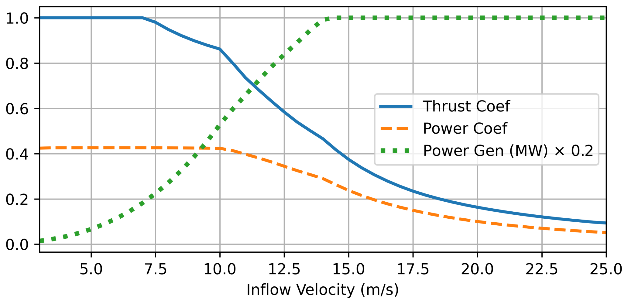
Figure 3 Thrust coefficient, power coefficient, and power generation as a function of inflow |U| for the NREL 5 MW lookup table computed with OpenFAST. The y axis units are non-dimensional for thrust and power coefficients, and scaled MW for power generation.

The lookup table was created by running the OpenFAST code (see http://github.com/OpenFAST/openfast, last access: 20 May 2025) using the NREL 5 MW turbine with the Aerodyn and Elastodyn modules using steady inflow with wind speeds increasing at integers of 3–25 m s⁻¹ to generate the thrust, power, and rotation rate values as a function of inflow wind speed at a density of 1 kg m⁻³. This increases the rated wind speed from its nominal value of 11.4 m s⁻¹. The ROSCO controller was used in this calculation. The thrust and power values were then translated into thrust and power coefficients using the actuator disk's swept area, and the square and cube of inflow velocity, respectively. The thrust coefficient is capped at a value of 1 to avoid flow reversal in the actuator disk parameterization.

Actuator disk approximation

A 1D momentum balance is used to approximate the thrust applied by rotating blades onto a flow (Madsen, 1996). The thrust deficit is given by

$$\begin{array}{}\text{(27)}& \mathit{T}\cdot \widehat{x}={\displaystyle \frac{\mathrm{1}}{\mathrm{2}}}\mathit{\rho }{C}_{\mathrm{T}}A\mathrm{|}U{\mathrm{|}}^{\mathrm{2}},\end{array}$$

where C_T is obtained from the table lookup, and $A=\mathit{\pi }{\left(D_{\mathrm{T}}/\mathrm{2}\right)}^{\mathrm{2}}$ is the area of the swept disk. D_T is the turbine disk diameter. A projection strategy is devised to relate the turbine parameterization to the dynamics on the computational grid. This total disk thrust is divided according to convex projection weights w_ijk (described in Appendix B2) to project thrust onto the flow. The indices i ,j, and k identify the discrete cell volume in the three dimensions, x, y, and z, respectively. Because the finite-volume method stores cell-averaged data, this thrust is then also divided by the cell volume ΔxΔyΔz in order to be applicable to cell-averaged quantities. Cell averages are indicated with an overbar. The update that introduces thrust and swirl is defined as

$$\begin{array}{}\text{(28)}& {\displaystyle }\begin{array}{rl}{\displaystyle \frac{\mathrm{d}{\stackrel{\mathrm{‾}}{\mathit{\rho }u}}_{ijk}}{\mathrm{d}t}}& =-{\displaystyle \frac{\mathrm{1}}{\mathrm{2}\mathrm{\Delta }x\mathrm{\Delta }y\mathrm{\Delta }z}}{C}_{\mathrm{T}}{\stackrel{\mathrm{‾}}{\mathit{\rho }}}_{ijk}\mathrm{|}U{\mathrm{|}}^{\mathrm{2}}\cos \left({\mathit{\theta }}_{\mathrm{yaw}}\right)\\ & \cdot A{w}_{ijk}-{\displaystyle \frac{\mathrm{1}}{\mathrm{2}\mathrm{\Delta }x\mathrm{\Delta }y\mathrm{\Delta }z}}{C}_Q{\stackrel{\mathrm{‾}}{\mathit{\rho }}}_{ijk}\mathrm{|}U{\mathrm{|}}^{\mathrm{2}}\sin \left({\mathit{\theta }}_{az}\right)\\ & \cdot \sin \left({\mathit{\theta }}_{\mathrm{yaw}}\right)A{w}_{ijk}\end{array}\text{(29)}& {\displaystyle }\begin{array}{rl}{\displaystyle \frac{\mathrm{d}{\stackrel{\mathrm{‾}}{\mathit{\rho }v}}_{ijk}}{\mathrm{d}t}}& =-{\displaystyle \frac{\mathrm{1}}{\mathrm{2}\mathrm{\Delta }x\mathrm{\Delta }y\mathrm{\Delta }z}}{C}_{\mathrm{T}}{\stackrel{\mathrm{‾}}{\mathit{\rho }}}_{ijk}\mathrm{|}U{\mathrm{|}}^{\mathrm{2}}\sin \left({\mathit{\theta }}_{\mathrm{yaw}}\right)\\ & \cdot A{w}_{ijk}+{\displaystyle \frac{\mathrm{1}}{\mathrm{2}\mathrm{\Delta }x\mathrm{\Delta }y\mathrm{\Delta }z}}{C}_Q{\stackrel{\mathrm{‾}}{\mathit{\rho }}}_{ijk}\mathrm{|}U{\mathrm{|}}^{\mathrm{2}}\sin \left({\mathit{\theta }}_{az}\right)\\ & \cdot \cos \left({\mathit{\theta }}_{\mathrm{yaw}}\right)A{w}_{ijk},\end{array}\text{(30)}& {\displaystyle \frac{\partial {\stackrel{\mathrm{‾}}{\mathit{\rho }w}}_{ijk}}{\partial t}}={\displaystyle \frac{\mathrm{1}}{\mathrm{2}\mathrm{\Delta }x\mathrm{\Delta }y\mathrm{\Delta }z}}{C}_Q{\stackrel{\mathrm{‾}}{\mathit{\rho }}}_{ijk}\mathrm{|}U{\mathrm{|}}^{\mathrm{2}}\cos \left({\mathit{\theta }}_{az}\right)A{w}_{ijk},\end{array}$$

where θ_yaw is the yaw angle of the turbine; ${\mathit{\theta }}_{az}={\tan }^{-\mathrm{1}}\left(z/-y\right)$ is the azimuth angle with respect to the hub center in reference space averaged over the cell; and $C_Q=C_{\mathrm{P}}U/\left(\mathrm{\Omega }{R}_{\mathrm{T}}\right)$ is the coefficient of torque, with $R_{\mathrm{T}}=D_{\mathrm{T}}/\mathrm{2}$ as the turbine radius and Ω as the rotation rate in radians per second obtained through a reference wind turbine table interpolation based on inflow speed. In the simulations that follow, the turbines are aligned with the mean flow, and cos (θ_yaw)=1. The portion of the total thrust that does not go into the production of power is injected into unresolved TKE:

$$\begin{array}{}\text{(31)}& {\displaystyle \frac{\mathrm{d}{\stackrel{\mathrm{‾}}{\mathit{\rho }K}}_{ijk}}{\mathrm{d}t}}=-{\displaystyle \frac{\mathrm{1}}{\mathrm{2}\mathrm{\Delta }x\mathrm{\Delta }y\mathrm{\Delta }z}}{C}_{\mathrm{T}}{\stackrel{\mathrm{‾}}{\mathit{\rho }}}_{ijk}\mathrm{|}U{\mathrm{|}}^{\mathrm{3}}A{w}_{ijk},\end{array}$$

where $C_{\mathrm{TKE}}=\frac{\mathrm{1}}{\mathrm{4}}\left(C_{\mathrm{T}}-C_{\mathrm{P}}\right)$ is the fraction of unused thrust that will contribute to unresolved TKE (Fitch et al., 2012; Bui et al., 2024; Archer et al., 2020). Instantaneous velocities are used to compute the thrust and TKE injection in Eqs. (28)–(31). A 30 s average of the inflow velocity at the axis of the disk is used when interpolating $C_{\mathrm{T}}^{\star }$, $C_{\mathrm{P}}^{\star }$, and P from the lookup table (see Fig. 3).

4.3 Details on the boundary layer initialization and experiment setups

The primary parameter in all of the calculations is the inflow speed. The operational wind speeds for the NREL 5 MW turbine span 3–25 m s⁻¹. We first consider the power output and wake deficit of a single turbine and then a simple multiple-turbine farm configuration. In the latter case, the turbines' wakes change the power output of waked turbines downstream.

For single-turbine simulations, we simulate with 10 different mean hub-height precursor wind speeds (5, 7, 9, 11, 13, 15, 17, 19, 21, and 23 m s⁻¹) with and without floating-platform motions added to the inflow velocity of the turbine actuator disk for three different turbulent intensities: 25 % of default (TI_0.25), 100 % of default (TI_1.0), and 200 % of default (TI_2.0) – all using the Betti et al. (2014) model for floating-platform motions. The default turbulence intensity for a given wind speed is that which naturally arises from a neutral ABL and the surface roughness length arising from the Charnock relation at a given hub-height wind speed. These TI values are shown as the last column in Table 1. Additionally, the effects of harmonic-forced floating-platform motions (rather than the motions induced by the wave-forced Betti et al. (2014) model) are evaluated at TI_1.0 for the 10 wind speeds with and without floating-platform motions. This leads to 80 total single-turbine simulations each for 8 model hours. For the multi-turbine simulations, a grid of three rows of 10 turbines (10 turbine diameters apart in both spanwise and streamwise horizontal directions) is simulated with TI_0.25 and an inflow average hub-height wind speed of 10 m s⁻¹ for 8 model hours. Due to downstream wake effects, an average inflow of around 7.5 m s⁻¹ was observed for the latter nine turbines.

For the single turbine we use a (length, height, width) $\mathrm{30}\times \mathrm{10}\times \mathrm{6.35}$ turbine diameters domain (where D is the turbine diameter) simulated for 8 model hours – the last 4 of which are used for analysis after the neutral ABL has spun up. For multi-turbine simulations, a domain of $\mathrm{130}\times \mathrm{40}\times \mathrm{6.35}$ turbine diameters is simulated for 8 model hours – the last 4 of which are used for analysis. Each turbulent precursor is forced with a uniform pressure gradient forcing that penalizes horizontal-mean deviations of hub-height wind speed from the intended mean value. The pressure gradient forcing calculated and used in the precursor is also applied to the turbine simulation to ensure the pressure gradient advances the flow physically. All simulations contain a dynamical core, an LES closure, and the application of surface friction to impose a roughness length determined by the Charnock relation for the given hub-height wind speed. The time step size used for all portions of the model (dynamical core, LES closure, wind turbine parameterization, surface friction, and floating-platform motion parameterization) is $\mathrm{\Delta }x{\left(u_{\max }\right)}^{-\mathrm{1}}\left(\mathrm{CFL}\right)=\mathrm{10}\mathrm{m}{\left(\mathrm{450}\mathrm{m}{\mathrm{s}}^{-\mathrm{1}}\right)}^{-\mathrm{1}}\left(\mathrm{0.6}\right)=\mathrm{1.33}\times {\mathrm{10}}^{-\mathrm{2}}\mathrm{s}$. For single-turbine simulations, the turbine is placed at 6 turbine diameters from the left x direction boundary and in the middle of the domain in the y direction. For multi-turbine simulations, the first column of turbines begins at 11 turbine diameters into the x direction of the domain, and the rows are 10 diameters apart and collectively centered in the y direction.

The neutral boundary layer is initialized with the following potential temperature profile:

$$\begin{array}{}\text{(32)}& \mathit{\theta }\left(z,t=\mathrm{0}\right)=\left\{\begin{array}{ll}\mathrm{300}& \mathrm{if}z<\mathrm{500}\mathrm{m}\\ \mathrm{300}+\mathrm{0.08}\left(z-\mathrm{500}\right)& \mathrm{if}\mathrm{500}\le z\le \mathrm{650}\\ \mathrm{312}+\mathrm{0.003}\left(z-\mathrm{650}\right)& \mathrm{if}z>\mathrm{650}.\end{array}\right.\end{array}$$

The velocity is initialized with a log-law of u velocity targeting the appropriate hub-height velocity for the individual experiment with $v=w=\mathrm{0}$. To initiate turbulence, potential temperature perturbations from a random uniform distribution $\in \left[-\mathrm{1},\mathrm{1}\right]$ are added to the lowest 100 m of the domain, and horizontal velocities are perturbed with 4-period sine functions in transverse directions.

The different turbulent intensities (TI_0.25, TI_1.0, and TI_2.0) are created by scaling wind velocity deviations from the mean column from the precursor simulation before applying it as inflow to the turbine simulations by 25 %, 100 %, and 200 %, respectively. These act to mimic turbulent intensities arising from transient stable and unstable boundary layers.

5 Numerical results and discussion

5.1 Turbine power and velocity – moving platform conditions

In what follows, we will refer to outcomes computed with no platform motions as Fixed. When the outcomes involve platform motions due to ocean dynamics, we will refer to the results as Moving/Ocean. A key feature of platform motions affected by a fully developed (Pierson–Moskowitz) ocean wave spectrum (see Stewart, 2008) is the assumption that the waves have zero-mean random phases. This is in contrast to induced platform motions due to swells created by distant disturbances and storms, which tend to have spectra with fixed or slowly changing phases. Consideration of swell conditions is outside of the scope of this study. However, we will explore a simpler case, namely a sinusoidal perturbation of the incoming wind, with a fixed phase. The significant wave height is used as the amplitude, and the peak Pierson–Moskowitz frequency is used as the frequency for the sinusoidal forcing – resulting in relatively large amplitude perturbations. We will denote the results of calculations with the oscillating perturbation as Moving/Oscillating.

We next describe the computation of U(t), to be used in the actuator disk approximation. For the fixed conditions case,

$$\begin{array}{}\text{(33)}& U\left(t\right)=u_{\mathrm{upstream}};\end{array}$$

and in the Moving/Ocean case:

$$\begin{array}{}\text{(34)}& U\left(t\right)=u_{\mathrm{upstream}}+u_{\mathrm{platform}}\left(t\right).\end{array}$$

The dynamics of u_platform(t) are described by Eq. (24), with input u_upstream at 10 m above the sea surface. The platform motions are described in Sect. 2. For Moving/Oscillating conditions, we have

$$\begin{array}{}\text{(35)}& U\left(t\right)=u_{\mathrm{upstream}}+A{\mathit{\omega }}_p\cos \left({\mathit{\omega }}_{p}t\right).\end{array}$$

The amplitude A is determined by the significant height (see Appendix A), and ω_p is the peak of the Pierson–Moskowitz spectrum generated by u_upstream at 19.5 m above the sea surface.

5.2 Velocity and power, Moving/Ocean conditions for a single turbine

In Table 1, we report the standard deviation of the components of U(t) (see Eqs. 24 and 34) as a function of incoming hub-height wind speed in the precursor inflow, under three inflow turbulent intensities. Platform-induced motions due to ocean and turbulent thrust motions increase as the standard deviation of u_upstream and the hub wind speed increases. In all regimes, the standard deviations of u_platform are much smaller than the standard deviations of u_upstream, meaning the fluctuations due to floating-platform motions are not significant compared to the already present turbulent intensity and are, therefore, expected to have relatively minor impact on wake deficit and downstream power generation.

Table 1 Standard deviation of u_platform and u_upstream over a range of hub-height wind speeds with different inflow turbulent intensities using Moving/Ocean conditions (see Eq. 34 for the platform over the last 4 h of an 8 h simulation). Turbulence intensity is computed as $\mathit{\sigma }\left(\mathrm{|}{\mathbf{u}}_{\mathrm{hub}}\mathrm{|}\right)/\mathit{\mu }\left(\mathrm{|}{\mathbf{u}}_{\mathrm{hub}}\mathrm{|}\right)$ from the precursor simulation at t=8 h.

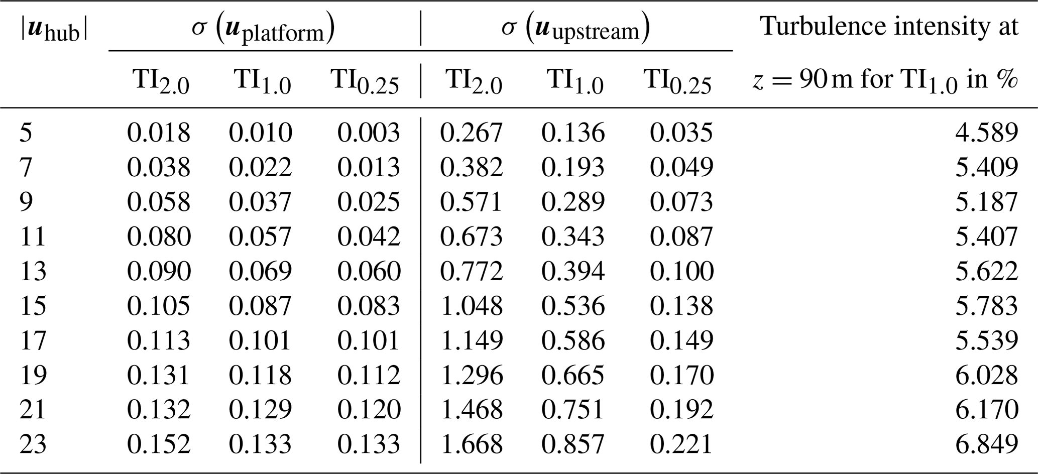
Figure 4 plots the ratio of Moving/Ocean x direction wind speed (disk-normal wind speed) averaged over the hub area and divided by that of the Fixed x direction wind speed averaged over the hub area, averaged over the last 4 h of simulations for mean precursor hub-height inflow speeds of 5, 7, 9, and 11 m s⁻¹, where power production is below rating. Figure 5 plots are the same, except the for y axis, which instead gives the ratio of power production according to the lookup table of |u|, as plotted in Fig. 4. For wind speeds higher than 11 m s⁻¹, the ratios are extremely small (order of 10⁻⁶ or smaller) because the turbines are already at rated wind speed, meaning the power differences are negligible.

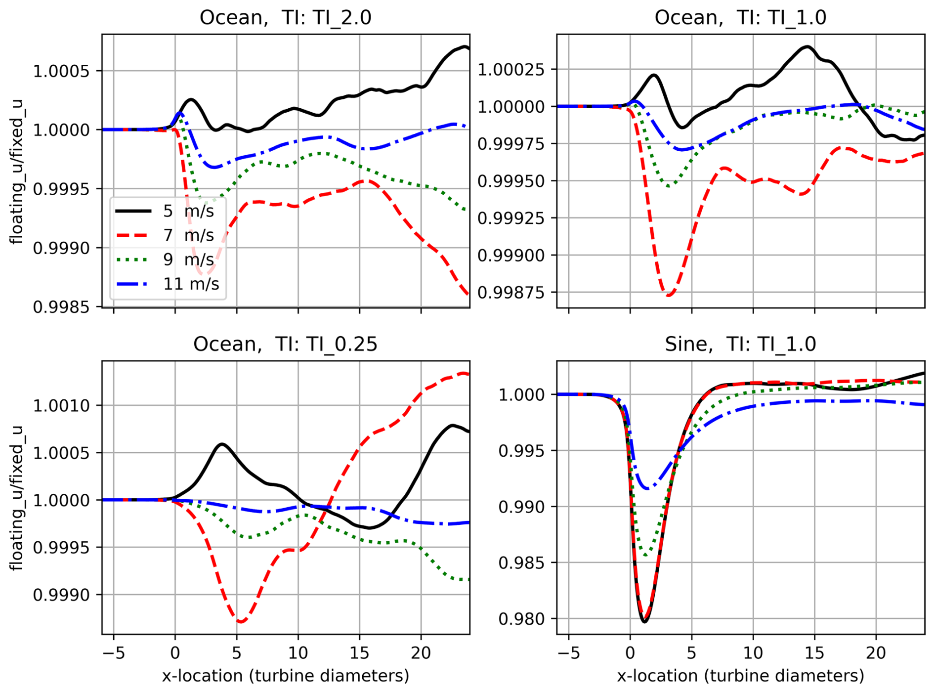
Figure 4 Ratio of averaged horizontal velocity magnitude of Moving/Ocean to Fixed conditions for hub-height wind speeds of 5, 7, 9, and 11 m s⁻¹. Averages are integrated over the last 4 h of simulation over the turbine diameter in the y direction, and over the turbine diameter in the z direction. The x axes are x direction in units of turbine diameter D. The y axes are dimensionless ratios. Note the different y axis scales in plots.

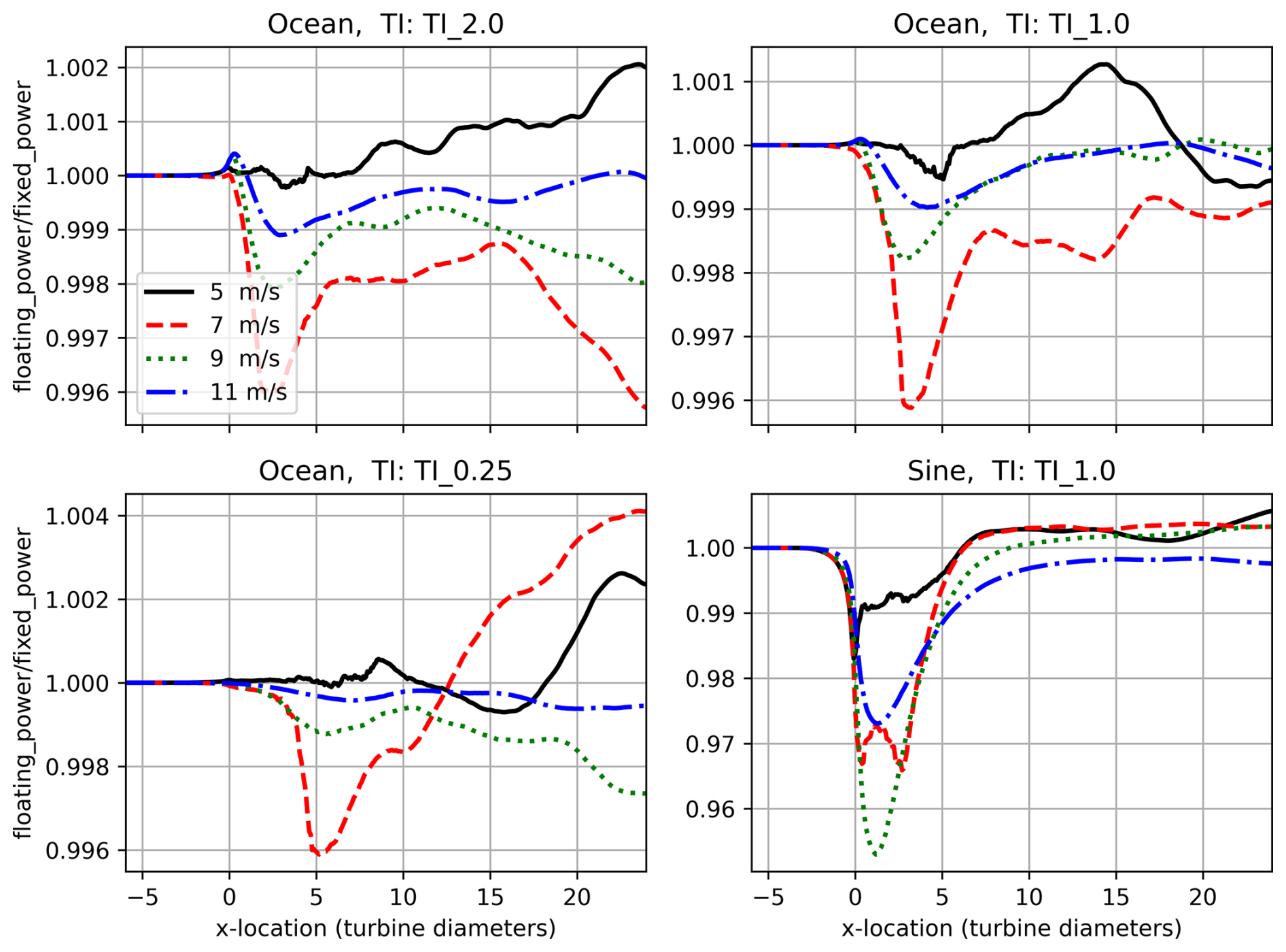
Figure 5 Ratio of averaged power production of Moving/Ocean to Fixed conditions for hub-height wind speeds of 5, 7, 9, and 11 m s⁻¹. Averages are integrated over the last 4 h of simulation over the turbine diameter in the y direction, and over the turbine diameter in the z direction. The x axes are x direction in units of turbine diameters. The y axes are dimensionless ratios. Note the different y axis scales in plots.

In all simulations, including single- and multi-turbine simulations, the power production of the turbines (and emulated power production by using the wake velocity as input to the reference turbine table to deduce power) mounted on floating platforms is within 1 % of the power production of fixed turbines. At 10 diameters downstream and onward, where another turbine is likely to be placed in a floating-platform offshore farm, the power production is within half a percent, comparing floating to fixed platform, with the larger differences occurring for lower wind speeds, where the power production is already relatively low. The wake deficit ratios between floating and fixed turbines are within 0.1 % for all wind speeds as well.

5.3 Motion effects on velocities for Moving/Sinusoidal conditions for a single turbine

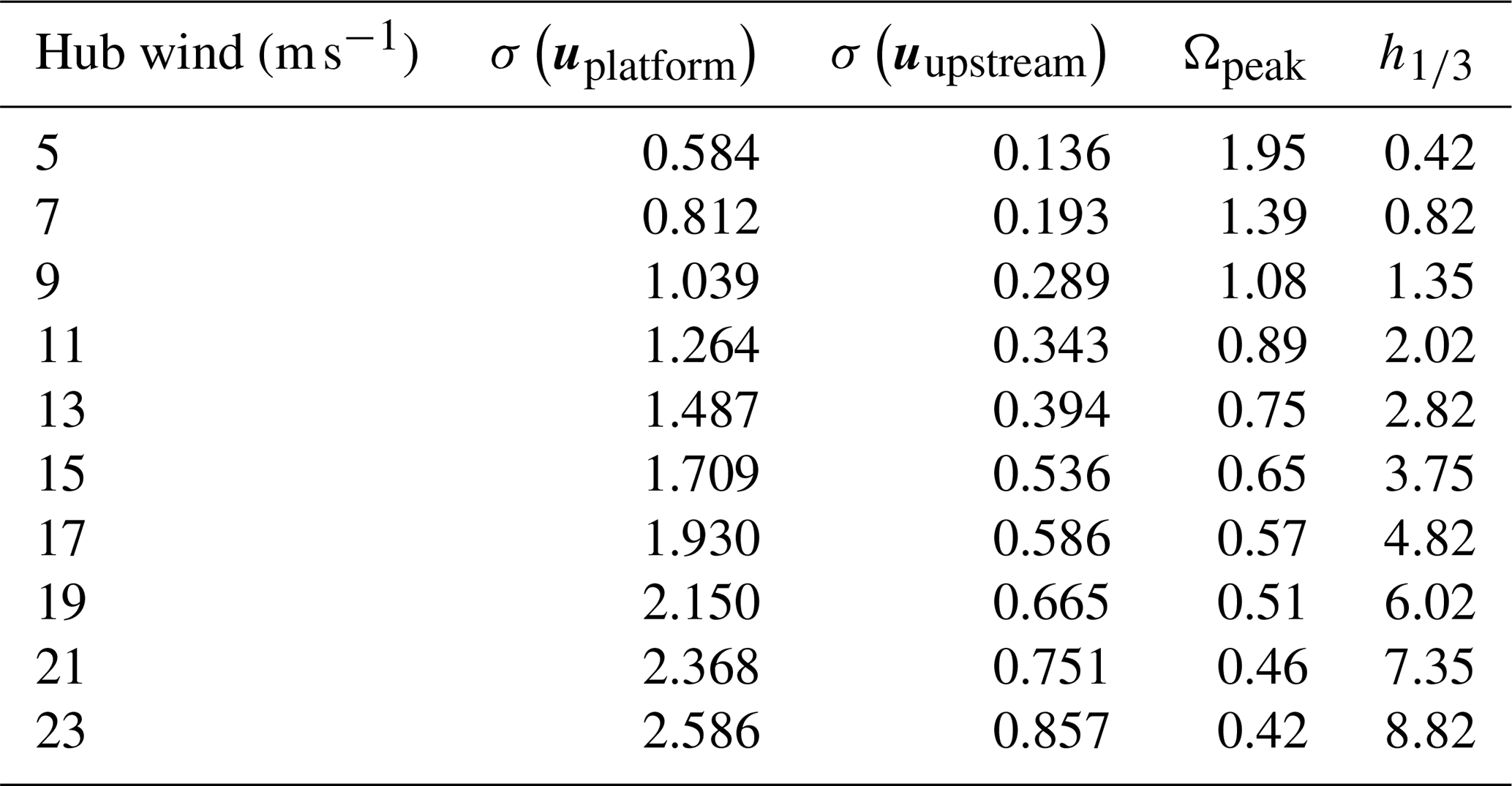
As a way to assess the extent to which our conclusions regarding floating-platform motion effects on power generation depend on the nature of the dynamics of the platform motion, in order to discern whether randomness explained the small effect of fully developed wave motions on the power output, we also submitted the platform to sinusoidal motions (see Eq. 35). For a given hub wind speed, we use the significant wave height as the amplitude of the sinusoidal and the peak frequency in the sine wave. The outcomes for each wind speed are summarized in Table 2 as well as in the bottom-right panels of Figs. 4 and 5. We test different turbulence intensities to emulate conditions that emerge from stable, neutral, and convective thermal stratifications. While the 10D downstream power generation differences due to floating-platform motions remains small (within 0.5 %–1 %), there is a significant effect in the very-near-wake region of 0–6 turbine diameters downstream due to Moving/Oscillating platform motions. As with the floating-platform-induced motions, the larger differences are confined to the near-wake region, where a downstream turbine is less likely to be placed in a farm configuration. For all wind speeds, the sinusoidal motion forcing leads to a decrease in power production in the near-wake region (less than 5 turbine diameters downstream). For lower wind speeds, the power production increases due to sinusoidal forcing in the far-wake region; and for larger wind speeds, the power production is decreased due to sinusoidal forcing in the far-wake region (both to modest degrees of less than half a percentage).

Table 2 Standard deviation of u_platform and u_upstream over a range of hub-height wind speeds in TI_0.25 conditions using Moving/Oscillating conditions (see Eq. 35) for the platform. Ω_peak is the peak frequency of the Pierson–Moskowitz approximation to a fully developed ocean used as the frequency for the oscillating forcing. $h_{\mathrm{1}/\mathrm{3}}$ is the “significant wave height” used as the amplitude for the oscillating forcing.

5.4 Velocity and power generation of a farm of turbines mounted on floating platforms, forced by ocean gravity waves

The question of whether floating-platform motions have an effect on the power output of a farm of turbines set on floating platforms is considered next. The turbine farm we consider has three rows of turbines (we consider a “row” to be a streamwise (x) direction series of 10 turbines), equally spaced and at equal heights, lined up with the wind in such a way as to produce the most direct interaction of upstream wakes with downstream turbines. We also give the turbine's “ID” in the streamwise (x) direction from 1 to 10, increasing in the positive x direction (positive streamwise direction). The atmosphere conditions use the TI_1.0 (or default neutral ABL) configuration, where floating-platform motions are relatively larger than turbulent fluctuations as compared to the other turbulent intensities. The sea is fully developed, and thus the platform motions due to the ocean waves of each turbine are not correlated with each other. One key difference between this farm simulation and the previous single-turbine simulations is that in this farm simulation, the turbine's yaw angle and upstream sampling direction are allowed to change in response to the flow for a more realistic view of how turbines might behave differently due to floating motions in a farm setting.

Each time step, the horizontal velocity is averaged within 1 turbine radius of the hub location to determine the upstream direction. The flow is sampled 2 turbine diameters upstream of the hub location using the exact same projection technique used to project thrust onto the flow in the actuator disk parameterization. The yaw angle also responds to this upstream direction by rotating toward the time-averaged upstream direction over a 1 min moving average window at a maximum rotation rate of 0.3° s⁻¹, as specified in the NREL 5 MW Offshore Wind Turbine Definition document (Jonkman et al., 2009).

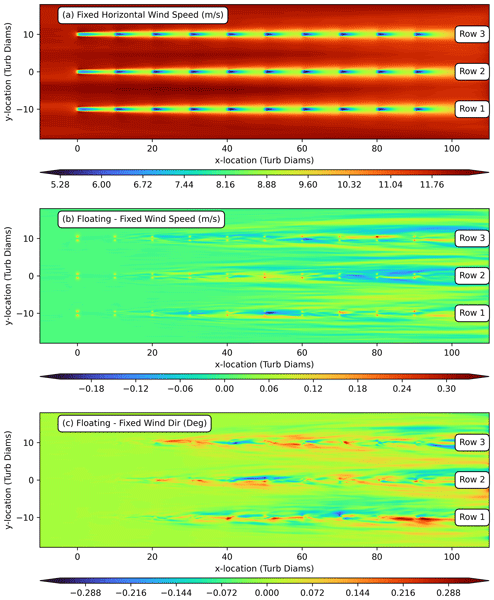
Figure 6 plots the time average over $t\in \left[\mathrm{5},\mathrm{10}\right]$ h and spatial average over $z\in \left[\mathrm{90}-\mathrm{63},\mathrm{90}+\mathrm{63}\right]$ m of (a) fixed-platform horizontal wind speed (in m s⁻¹); (b) fixed-platform horizontal wind speed subtracted from floating-platform horizontal wind speed (in m s⁻¹); and (c) fixed-platform wind direction subtracted from floating-platform wind direction (in degrees). The initial turbines in the streamwise direction (turbines with ID 1 in rows 1, 2, and 3) receive the largest inflow wind speed. Due to the waking of downstream turbines, the downstream turbines receive lower inflow wind speeds. Also, wakes expand in the horizontal spanwise direction (y direction) as expected as the flow progresses in the streamwise direction (positive x direction). Initially (at the negative x direction boundary), the differences between floating and fixed horizontal wind speed and direction are zero due to shared precursor inflow conditions. The differences slowly develop over the first and second turbine wakes in each row, the wind direction exhibits abrupt changes in the third turbine of each row, and the wind speed differences develop more slowly when progressing in the streamwise direction.

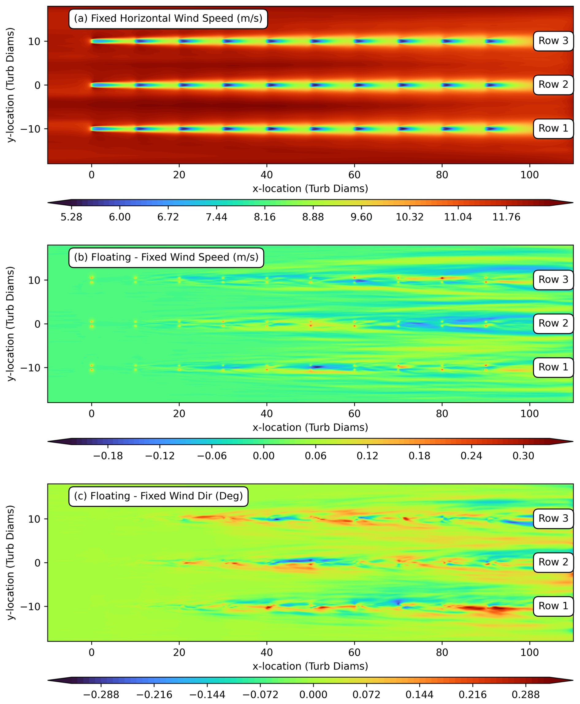
Figure 6 Contour plots of time average over $t\in \left[\mathrm{5},\mathrm{10}\right]$ h and spatial average over $z\in \left[\mathrm{90}-\mathrm{63},\mathrm{90}+\mathrm{63}\right]$ m of (a) fixed-platform horizontal wind speed (in m s⁻¹); (b) fixed-platform horizontal wind speed subtracted from floating-platform horizontal wind speed (in m s⁻¹); and (c) fixed-platform wind direction subtracted from floating-platform wind direction (in degrees).

Pressure-gradient-forced ABLs are known to exhibit streamwise “streaks” in the wind field that differ in the horizontal spanwise direction and persist even over long time averages (Pimont et al., 2020). These are visible in Fig. 6a on the left-hand side of the plot (the turbulent precursor inflow). The floating motions lead to minute time-mean differences in wake behavior at the first turbine of each row, which would be experienced even with small random noise due to the chaotic divergence of initially close solutions exhibited in any turbulent fluid flow. These minute wake changes due to floating motions are then modulated by persistent streaks in the pressure gradient, forced to lead to time-persisting changes in yaw angle. The altered yaw angle then steers the flow, which, coupled with further chaotic divergence in the floating versus fixed solutions, leads to larger changes in flow speed and direction as one progresses downstream. The changes are on the order of 1 % relative magnitude or less in terms of inflow speed at each of the turbines. This leads to greater changes in power production on the order of 3 % or less in relative magnitude, since the power production scales with the cube of the inflow wind speed.

To observe this in a different format, Fig. 7 plots the time average over $t\in \left[\mathrm{5},\mathrm{10}\right]$ h and spatial average over $z\in \left[\mathrm{90}-\mathrm{63},\mathrm{90}+\mathrm{63}\right]$ m for each individual turbine of (a) floating-to-fixed platform power production, (b) floating-to-fixed platform inflow wind speed normal to the disk, and (c) floating-to-fixed platform yaw angle (degrees). Figure 7d plots the fixed-platform inflow wind speed for each turbine with the same averaging in space and time. From these plots, it is clear that at the first turbine in each row, the differences in power production, inflow wind speed, yaw angle, and yaw misalignment are all nearly zero and slowly develop over the first three turbines before saturating at larger differences in downstream turbines. This supports the mechanism of chaotic divergence of initially close solutions due to small perturbations from floating motions building in the streamwise direction. With this in mind, even with persistent streaks in the precursor, the mean relative difference in power production over all of the turbines is 0.27 %. This is roughly 3× larger in magnitude than the single-turbine relative power differences at different turbulence intensities at 10 turbine diameters downstream in Fig. 5 using the 9 m s⁻¹ inflow curve, as the mean inflow over most of the turbines in between 9 and 9.5 m s⁻¹ in the farm case. Therefore, while progressive chaotic divergence in the floating versus fixed solutions coupled with active yawing and pressure-gradient-based streaks leads to a difference in the farm's power response, it is not different by an order of magnitude. Further, in the single-turbine case, the power difference is slightly lower due to floating motions by roughly 0.1 % at 10 turbine diameters downstream, while in the farm case, the power generation averaged over all of the turbines is slightly larger, by 0.27 %, due to floating motions.

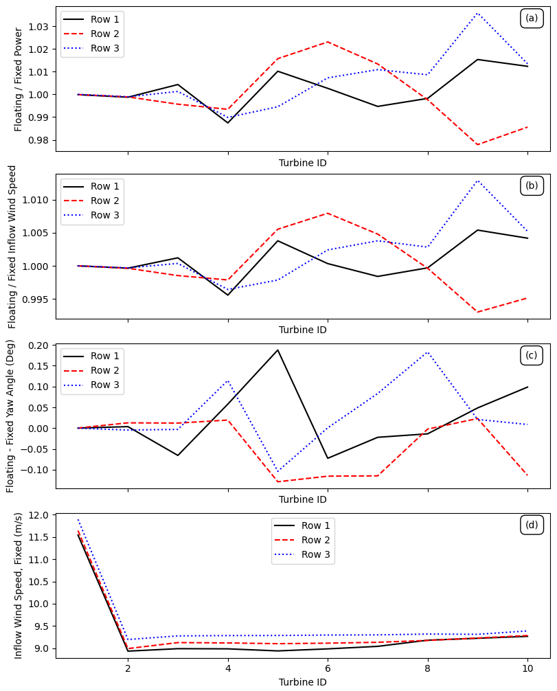
Figure 7 Time averages over $t\in \left[\mathrm{5},\mathrm{10}\right]$ h and spatial average over $z\in \left[\mathrm{90}-\mathrm{63},\mathrm{90}+\mathrm{63}\right]$ m for each individual turbine of (a) floating-to-fixed platform power production; (b) floating-to-fixed platform inflow wind speed normal to the disk; (c) floating-to-fixed platform yaw angle (degrees); (d) plots the fixed-platform inflow wind speed for each turbine with the same averaging in space and time.

Figure 8 depicts the (floating-to-fixed conditions) relative power time series and its cumulative average corresponding to the right-most turbine (ID 10) in each row. This plot demonstrates that, over $t\in \left[\mathrm{5},\mathrm{10}\right]$ h, the flow has reached a state of equilibrium amid the higher frequency oscillations, as the ratio in power production is not drifting. This indicates that our long-term average power estimates are stationary and thus robust. Plots of the same quantity for the single FOWT cases will show the same stationary behavior.

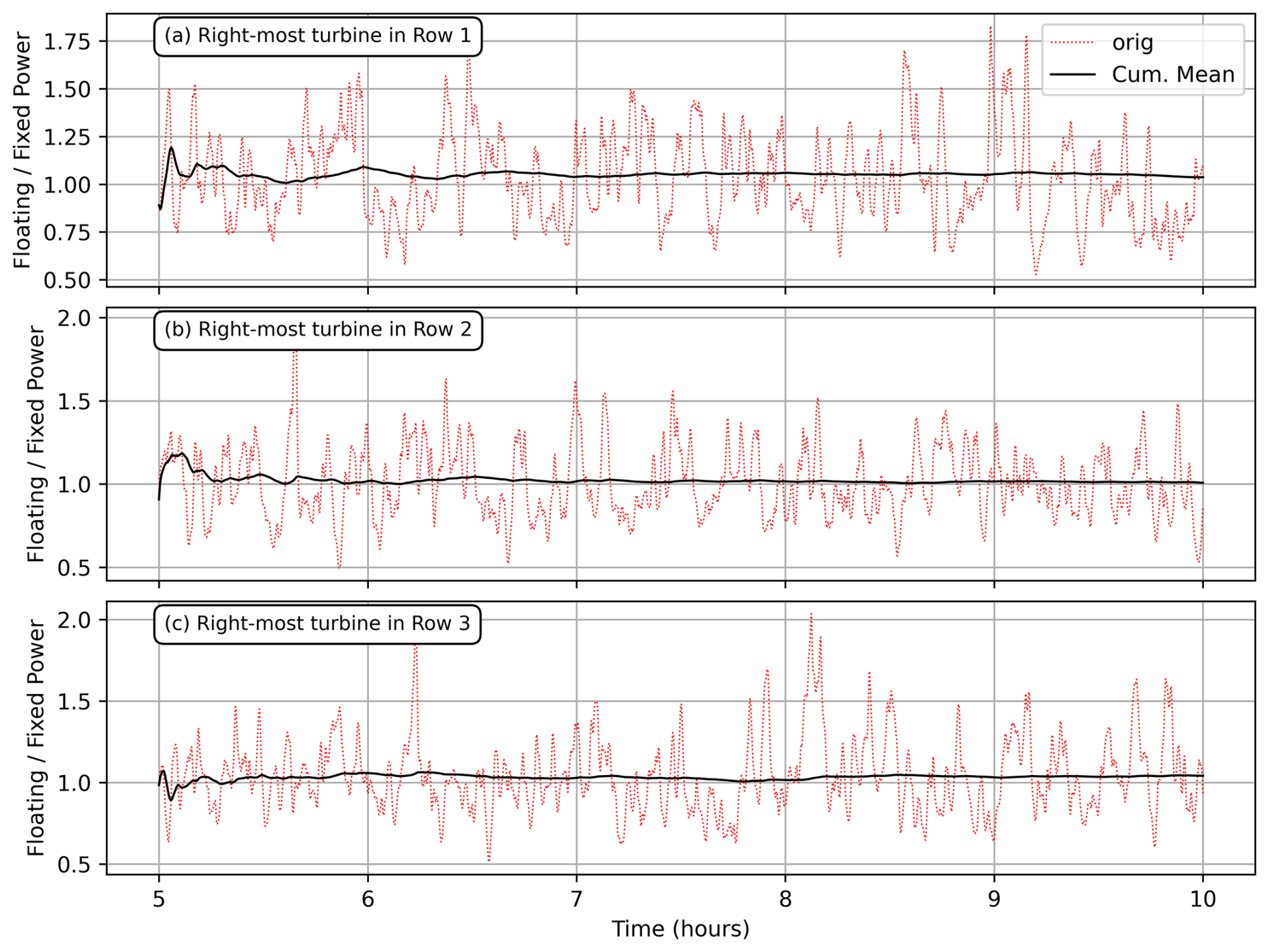
Figure 8 Floating-to-fixed relative power time series and its cumulative mean. Data taken from the right-most turbine (ID 10) in each row. The cumulative mean settles quickly, well before the span we take in averaging power outputs.

6 Conclusions

We used simulations to assess how the power output of a single wind turbine, 5 MW NREL, mounted on a floating tension-leg platform as well as well as that of a cluster of the same, are affected by ocean wave motions. This assessment was done by comparing the time-averaged power of the floating-platform ocean turbines to the same wind conditions while not allowing the platform to move by oceanic disturbances.

The simulations consisted of a wind, captured by large-eddy simulations (Norman, 2021) of an atmosphere with three inflow turbulence intensities; a mechanical model of a floating chain-stabilized tension-leg platform due to Betti et al. (2014); and a time-dependent empirical model for fully developed wind waves described by the Pierson–Moskowitz spectrum (see Stewart, 2008). The dynamics of the platform, the turbines, the ocean waves and the atmosphere are coupled. The specific turbine was the NREL 5 MW design. Platforms are often motion stabilized; however, we did not take into account any active motion stabilization and control dynamics. The three turbulence intensities act as a means to understand whether the results in this study are dependent upon the pre-existing turbulence intensity, typically modulated by surface roughness length and buoyant stability of the mean atmospheric profile.

For an isolated turbine mounted on a floating platform subjected to waves, we found that the platform motions due to a fully developed ocean minimally affected the wake deficits downstream. Further, the time-averaged downstream power production was not affected in a significant way by ocean-induced and intermittent thrust-induced platform motions. The floating-platform motion-induced perturbations to inflow velocity are quite small compared to already existing turbulent intensity, even at 25 % of the naturally occurring neutral boundary layer turbulence, which is the primary reason why observed changes to wake deficits and downstream power generation due solely to floating-platform motions are small.

Figure 9 depicts the power spectrum of u_platform and u_upstream for neutral atmospheric conditions and the Moving/Ocean platform configuration, with a hub speed of 11 m s⁻¹ and fully developed ocean wave conditions. From this figure, we surmise that the spectrum of U(t) is dominated by platform motions in the high-frequency regime and by the wind turbulence in the low-frequency regime. Furthermore, the most energetic part of the spectrum is associated with wind dynamics and turbulence. The sharp spectral peak and trough originate in the vibrational character of the particular floating platform under consideration, and thus one cannot conclude that this structure will appear in the spectra of other floating-platform arrangements. Regarding power generation assessments and whether differences in power output are significant for a fixed or moving platform, the spectra indicate that if power difference assessments are made at sufficiently long times, well over hundreds of seconds, the average power output is dominated by the wind contribution, not the combined wind/platform contribution. The random-phase nature of the waves and the dominance of the wind dynamics on U(t) over platform motions suggest that under fully developed ocean conditions, neither the single turbine mounted on a floating platform nor organized clusters of turbines of the type we investigated are affected in a significant way regarding power generation by ocean motions. Long time averages of the platform acceleration was zero, and therefore it was not expected to see, in the average, a net increase or decrease in the power output of a single turbine. However, it was not obvious at the onset that in cluster arrangements the platform dynamics would affect the wake of windward turbines and thus affect the power of the turbines downstream. However, our calculations reveal that downwind turbines are not appreciably affected by average power output. Wake disturbances were clearly apparent on turbines subjected to wave motions; however, this was at near distances that are outside of the realm of practicality.

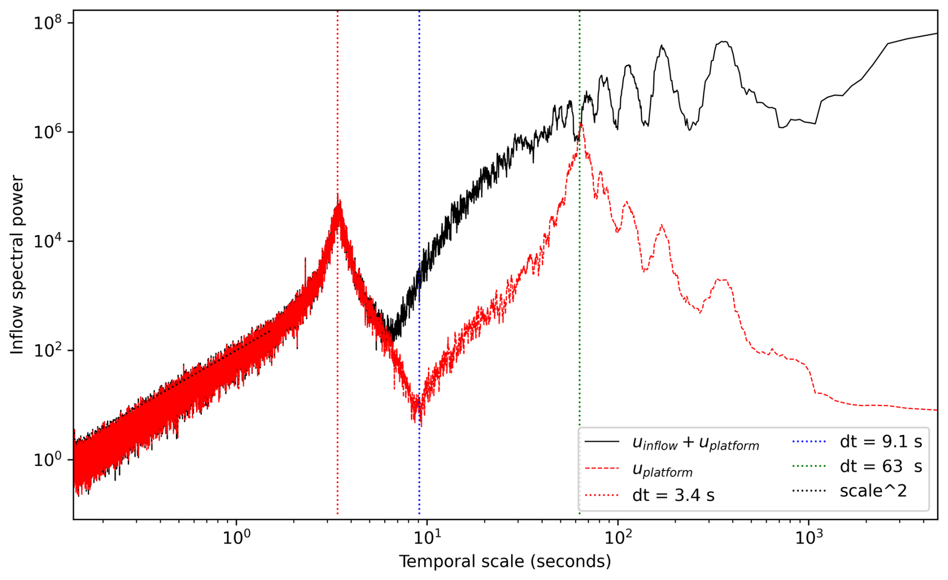
Figure 9 Power spectra in time of the magnitude of u_platform(t) and u_platform+u_inflow as a function of time scale (inverse frequency) at a hub wind speed of 11 m s⁻¹, with TI_1.0 inflow with a smoothing window of 10 samples for clarity. All hub wind speeds and stability profiles share the same local extrema for u_platform.

As a check, we compared random ocean perturbations to (zero-mean) sinusoidal fluctuations of the hub speed in order to determine whether random effects in the platform dynamics had a crucial role to play in enhancing/suppressing the time-averaged power output of a moving turbine, as compared to pure sinusoidal fluctuations of the hub speed. We found that, for reasonable sinusoidal amplitude and frequency perturbations, there was little change on the power output of the turbine in the far wake, although downstream power production is lowered in the near wake where downstream turbines are unlikely to be placed.

Wind waves modeled by the Pierson–Moskowitz (PM) spectrum – and for developing seas, the JONSWAP model – represent the vast majority of wave types in deep waters; however, the model assumptions are seldom perfectly realized in nature: the PM spectrum defines a “fully developed sea”, requiring wind to blow steadily at a constant speed over considerable distances and time. Because these perfect, uninterrupted conditions seldom occur naturally, the PM spectrum serves more as a foundational theoretical limit. Despite this, the PM spectrum is extensively utilized in ocean engineering and naval architecture as it represents the absolute worst-case equilibrium for a specific wind speed, providing engineers with a conservative, standardized benchmark for designing the structural integrity of ships, oil rigs, and floating platforms.

A full assessment of the effects of wave motions on the power output of turbines mounted on moving platforms necessitates consideration of transient dynamics. As a first step, we argue, it is critical to consider how multi-spectral wind waves affect the power output of FOWTs. Some of the transient conditions to consider next are obvious: the effect of swells, changing wind conditions and storms, and developing or decaying ocean waves. Some are less obvious. For example, finite-time averages of power output could still be affected by a fully developed ocean: when the hub wind dips up and down around the minimum or maximum wind operating conditions, for example, or when wind directions are not well accounted for by an alignment of the wind and the turbine. Nevertheless, for moored platforms like the TLP design studied here, under the most generic of ocean conditions, namely sustained steady winds and a fully developed ocean, the power of floating ocean turbines does not appear, in simulations, to be affected significantly when compared to fixed turbines. The consideration of transient wave effects on power output necessitates the consideration of the types of waves and conditions found in actual geographical locations of interest to be meaningful. Our simulation framework takes as a prescribed forcing the sea wave models; hence, in principle, the formulation is easily extensible to consider transient wave cases.

Appendix A: Fully developed sea conditions

The fully developed sea surface wind waves are captured by the Pierson–Moskowitz (PM) spectrum model (Stewart, 2008; Pierson and Moskowitz, 1964). The PM spectrum takes as input the steady wind speed at a height of 19.5 m above the mean sea surface and is given by

$$\begin{array}{}\text{(A1)}& S_{\mathrm{PM}}\left(\mathit{\nu }\right)={\displaystyle \frac{\mathrm{0.0081}{g}^{\mathrm{2}}}{(\mathrm{2}\mathit{\pi }{)}^{\mathrm{4}}{\mathit{\nu }}^{\mathrm{5}}}}{e}^{-\frac{\mathrm{5}}{\mathrm{4}}(\frac{\mathit{\nu }}{{\mathit{\nu }}_{\mathrm{peak}}}{)}^{-\mathrm{4}}},\end{array}$$

where $\mathrm{2}\mathit{\pi }{\mathit{\nu }}_{\mathrm{peak}}=\mathrm{0.877}g/u_{\mathrm{19.5}}$, u_19.5 is the wind speed at a 19.5 m height above the sea surface, g is acceleration, and ν is frequency. To obtain a random realization, we choose a frequency range of width Δν, the amplitude a_i of the monochromatic wave with angular frequency Ω_i=2πν_i is $a_i=\sqrt{\mathrm{2}{S}_{\mathrm{PM}}\left({\mathit{\nu }}_i\right)\mathrm{\Delta }{\mathit{\nu }}_i}$, where ν_i is the central frequency of the interval Δν. The sea elevation $z=\mathit{\eta }(x_p,t)$ is given by

$$\begin{array}{}\text{(A2)}& \begin{array}{rl}\mathit{\eta }(x_p,t)& =\sum _{i=\mathrm{1}}^N{a}_i\sin ({\mathrm{\Omega }}_{i}t-k_i{x}_p+{\mathit{ϵ}}_i),\\ \ddot{\mathit{\eta }}& =-\sum _{i=\mathrm{1}}^N{\mathrm{\Omega }}_i^{\mathrm{2}}{a}_i\sin ({\mathrm{\Omega }}_{i}t-k_i{x}_p+{\mathit{ϵ}}_i),\end{array}\end{array}$$

where x_p is the x location of the floating platform, ϵ_i is a random-phase ${\mathrm{\Omega }}_i=\sqrt{g{k}_i}$ for deep-water waves, and N is the number of spectral components, chosen at 400. For the wave forcing, we require u_19.5 to calculate the PM spectrum. This wind speed is taken as the cell average estimate from the large-eddy simulation calculation of the wind field, at a height of 19.5 m above the sea surface. The significant wave height, which is used to set A in Eq. (35), is given by

$$\begin{array}{}\text{(A3)}& A:=H_{\mathrm{1}/\mathrm{3}}=\mathrm{0.21}{\displaystyle \frac{u_{\mathrm{19.5}}^{\mathrm{2}}}{g}}.\end{array}$$

Appendix B: The large-eddy simulation model equations and its numerical implementation

The equations are cast in Cartesian geometry as follows:

$$\begin{array}{c}\text{(B1)}& {\displaystyle }{\partial }_t\mathbf{q}+{\partial }_x\mathbf{f}+{\partial }_y\mathbf{g}+{\partial }_z\mathbf{h}=\mathbf{s}{\displaystyle }\mathbf{q}=\left[\begin{array}{c}\mathit{\rho }\\ \mathit{\rho }u\\ \mathit{\rho }v\\ \mathit{\rho }w\\ \mathit{\rho }\mathit{\theta }\\ \mathit{\rho }{q}_{\mathrm{v}}\\ \mathit{\rho }K\\ \mathit{\rho }{q}_{\mathrm{\ell }}\end{array}\right],\mathbf{f}=\left[\begin{array}{c}\mathit{\rho }u\\ \mathit{\rho }uu+p+{\mathit{\tau }}_{\mathrm{11}}\\ \mathit{\rho }uv+{\mathit{\tau }}_{\mathrm{21}}\\ \mathit{\rho }uw+{\mathit{\tau }}_{\mathrm{31}}\\ \mathit{\rho }u\mathit{\theta }+{\mathit{\tau }}_{\mathit{\theta }\mathrm{1}}\\ \mathit{\rho }u{q}_{\mathrm{v}}+{\mathit{\tau }}_{\mathrm{v}\mathrm{1}}\\ \mathit{\rho }uK+{\mathit{\tau }}_{K\mathrm{1}}\\ \mathit{\rho }u{q}_{\mathrm{\ell }}+{\mathit{\tau }}_{\mathrm{\ell }\mathrm{1}}\end{array}\right],\\ \text{(B2)}& {\displaystyle }\mathbf{g}=\left[\begin{array}{c}\mathit{\rho }v\\ \mathit{\rho }vu+{\mathit{\tau }}_{\mathrm{12}}\\ \mathit{\rho }vv+p+{\mathit{\tau }}_{\mathrm{22}}\\ \mathit{\rho }vw+{\mathit{\tau }}_{\mathrm{32}}\\ \mathit{\rho }v\mathit{\theta }+{\mathit{\tau }}_{\mathit{\theta }\mathrm{2}}\\ \mathit{\rho }v{q}_{\mathrm{v}}+{\mathit{\tau }}_{\mathrm{v}\mathrm{2}}\\ \mathit{\rho }vK+{\mathit{\tau }}_{K\mathrm{2}}\\ \mathit{\rho }v{q}_{\mathrm{\ell }}+{\mathit{\tau }}_{\mathrm{\ell }\mathrm{2}}\end{array}\right]\text{(B3)}& {\displaystyle }\mathbf{h}=\left[\begin{array}{c}\mathit{\rho }w\\ \mathit{\rho }wu+{\mathit{\tau }}_{\mathrm{13}}\\ \mathit{\rho }wv+{\mathit{\tau }}_{\mathrm{23}}\\ \mathit{\rho }ww+p^{\prime }+{\mathit{\tau }}_{\mathrm{33}}\\ \mathit{\rho }w\mathit{\theta }+{\mathit{\tau }}_{\mathit{\theta }\mathrm{3}}\\ \mathit{\rho }w{q}_{\mathrm{v}}+{\mathit{\tau }}_{\mathrm{v}\mathrm{3}}\\ \mathit{\rho }wK+{\mathit{\tau }}_{K\mathrm{3}}\\ \mathit{\rho }w{q}_{\mathrm{\ell }}+{\mathit{\tau }}_{\mathrm{\ell }\mathrm{3}}\end{array}\right],\mathbf{s}=\left[\begin{array}{c}\mathrm{0}\\ \mathrm{0}\\ \mathrm{0}\\ -{\mathit{\rho }}^{\prime }g\\ \mathrm{0}\\ \mathrm{0}\\ K_{\mathrm{S}}+K_{\mathrm{D}}+K_{\mathrm{B}}\\ \end{array}\right]\text{(B4)}& {\displaystyle }p=\left({\mathit{\rho }}_{\mathrm{d}}{R}_{\mathrm{d}}+{\mathit{\rho }}_{\mathrm{v}}{R}_{\mathrm{v}}\right)T=C_{\mathrm{0}}{\left(\mathit{\rho }\mathit{\theta }\right)}^{\mathit{\gamma }},\end{array}$$

where ρ is density; u, v, and w are wind velocities in the x, y, and z directions, respectively; θ is the potential temperature; q_v is the wet water vapor mixing ratio such that ρ_v=ρq_v is the density of water vapor; K is unresolved, sub-grid-scale turbulent kinetic energy (TKE); q_ℓ is a tracer quantity that contributes to mass but not to pressure; p is total pressure; $C_{\mathrm{0}}={\left(R_{\mathrm{d}}{\left(p_{\mathrm{0}}\right)}^{-R_{\mathrm{d}}/c_p}\right)}^{\mathit{\gamma }}$ is a constant of proportionality; $\mathit{\gamma }=c_p/c_{\mathrm{v}}$ is the ratio of specific heats of dry air; c_p is specific heat of dry air at constant pressure; c_v is specific heat of dry air at constant volume; p₀ is reference pressure; R_d is the dry air ideal gas constant; R_v is the water vapor ideal gas constant; K_S is TKE shear production; K_D is TKE dissipation; K_B is the TKE buoyancy source/sink; τ_ij $\forall i,j\in \left\{\mathrm{1},\mathrm{2},\mathrm{3}\right\}$ is the unresolved eddy flux of wind velocity; τ_θj $\forall j\in \left\{\mathrm{1},\mathrm{2},\mathrm{3}\right\}$ is eddy flux of potential temperature; τ_vj is the eddy flux of water vapor; τ_Kj is the eddy flux of TKE (i.e., the turbulent transport terms for TKE); τ_ℓj is the eddy flux of tracers that do not contribute to pressure (e.g., hydrometeors); and g is acceleration due to gravity. Finally, the total density ρ is given by the sum of all mass-contributing densities: $\mathit{\rho }={\mathit{\rho }}_{\mathrm{d}}+{\mathit{\rho }}_{\mathrm{v}}+{\sum }_{\mathrm{\ell }}{\mathit{\rho }}_{\mathrm{\ell }}$, where ρ_d is the density of dry air.

The perturbation pressure $p^{\prime }=p-p_H$ and density ${\mathit{\rho }}^{\prime }=\mathit{\rho }-{\mathit{\rho }}_H$ are perturbations from a dominant hydrostatic balance, denoted by

$$\begin{array}{}\text{(B5)}& {\displaystyle \frac{\mathrm{d}{p}_H}{\mathrm{d}z}}=-{\mathit{\rho }}_{H}g.\end{array}$$

A semi-discretized, cell-centered, upwind finite-volume discretization is used in space with 9th-order-accurate weighted essentially non-oscillatory (WENO) reconstruction (Liu et al., 1994) with weight mapping (Henrick et al., 2005) for tracers and standard 9th-order Vandermonde-constrained polynomials for density and velocity. A 3rd-order-accurate, three-stage strong stability preserving (SSP) Runge–Kutta (RK) is used to discretize in time (see Gottlieb, 2005). In all simulations, a Courant–Friedrichs–Lewey stability value of CFL =0.6 is used, and a grid spacing of 10 m in each direction is implemented. Identical turbulent precursor inflow conditions are used for all simulations of a given hub-height mean wind speed to ensure that the only wake and power differences between simulations with and without floating-platform motions are due solely to floating-platform motions.

The model, including all turbine and floating-platform motion parameterizations, are coded in portable C++ using the Yet Another Kernel Launcher (YAKL) library (Norman et al., 2023a), a library based on the Kokkos (Trott et al., 2022) portability library, to run on CPUs or Nvidia, AMD, and Intel GPUs.

The eddy fluxes:

The eddy viscosity is considered to be a function of the unresolved TKE and a stability-corrected length scale, giving an eddy flux of

$$\begin{array}{}\text{(B6)}& {\displaystyle }\begin{array}{rl}& {\mathit{\tau }}_{ij}=-\mathit{\rho }\left(K_m+\mathit{\nu }\right)\left({\displaystyle \frac{\partial u_i}{\partial x_j}}+{\displaystyle \frac{\partial u_j}{\partial x_i}}-{\displaystyle \frac{\mathrm{2}}{\mathrm{3}}}{\displaystyle \frac{\partial u_k}{\partial x_k}}{\mathit{\delta }}_{ij}\right);\\ & \forall i,j,k\in \left\{\mathrm{1},\mathrm{2},\mathrm{3}\right\}\end{array}\text{(B7)}& {\displaystyle }{\mathit{\tau }}_{\mathit{\theta }j}=-\mathit{\rho }\left({\displaystyle \frac{K_m}{{\mathit{Pr}}_{\mathrm{T}}}}+{\displaystyle \frac{\mathit{\nu }}{\mathit{Pr}}}\right){\displaystyle \frac{\partial \mathit{\theta }}{\partial x_j}};\forall j\in \left\{\mathrm{1},\mathrm{2},\mathrm{3}\right\}\text{(B8)}& {\displaystyle }{\mathit{\tau }}_{Kj}=-\mathrm{2}\mathit{\rho }\left(K_m+\mathit{\nu }\right)\left({\displaystyle \frac{\partial K}{\partial x_j}}\right);\forall j\in \left\{\mathrm{1},\mathrm{2},\mathrm{3}\right\}\text{(B9)}& {\displaystyle }{\mathit{\tau }}_{\mathrm{\ell }j}=-\mathrm{2}\mathit{\rho }\left({\displaystyle \frac{K_m}{{\mathit{Pr}}_{\mathrm{T}}}}+{\displaystyle \frac{\mathit{\nu }}{\mathit{Pr}}}\right)\left({\displaystyle \frac{\partial {\mathit{\rho }}_{\mathrm{\ell }}}{\partial x_j}}\right);\forall j\in \left\{\mathrm{1},\mathrm{2},\mathrm{3}\right\}\text{(B10)}& {\displaystyle }{K}_m=\mathrm{0.1}L\sqrt{K}\text{(B11)}& {\displaystyle }{\mathit{Pr}}_{\mathrm{T}}={\displaystyle \frac{\mathrm{\Delta }}{\mathrm{1}+\mathrm{2}L}}\text{(B12)}& {\displaystyle }L=min\left({\displaystyle \frac{\mathrm{0.76}\sqrt{K}}{N+\mathit{ϵ}}},\mathrm{\Delta }\right)\text{(B13)}& {\displaystyle }\mathrm{\Delta }={\left(\mathrm{\Delta }x\mathrm{\Delta }y\mathrm{\Delta }z\right)}^{\mathrm{1}/\mathrm{3}}\text{(B14)}& {\displaystyle }N=\left\{\begin{array}{ll}\sqrt{\left(g/\mathit{\theta }\right)\left(\partial \mathit{\theta }/\partial z\right)}& \mathrm{if}\partial \mathit{\theta }/\partial z>\mathrm{0}\\ \mathrm{0}& \mathrm{otherwise}\end{array}\right.\end{array}$$

where $\mathit{ϵ}={\mathrm{10}}^{-\mathrm{20}}$ is a small number to avoid division by zero; N is the Brunt–Vaisala frequency, a measure of atmospheric stability; Pr_T is the turbulent Prandtl number; Pr is the Prandtl number; ν is kinematic viscosity; δ_ij is the Kronecker delta; u₁, u₂, and u₃ are the velocity components in the x, y, and z directions, respectively (i.e., u, v, and w); x₁, x₂, and x₃ are the x, y, and z directions, respectively; and subset indices that appear only on one side of an equation are an implied sum over available indices (Einstein summation convention).

TKE sources and sinks:

The TKE evolution equation contains advection and turbulent transport (diffusion) on the left-hand-side of Eq. (B1). The remaining processes resolved here are the sources and sinks that are, in general, not cast in conservation form. They are defined as

$$\begin{array}{}\text{(B15)}& {\displaystyle }{K}_{\mathrm{S}}=\mathit{\rho }{K}_m\sum _{i,j\in \left\{\mathrm{1},\mathrm{2},\mathrm{3}\right\}}\left({\displaystyle \frac{\partial u_i}{\partial x_j}}+{\displaystyle \frac{\partial u_j}{\partial x_i}}\right){\displaystyle \frac{\partial u_j}{\partial x_i}}\text{(B16)}& {\displaystyle }{K}_{\mathrm{D}}=-\mathit{\rho }\left(\mathrm{0.19}+\mathrm{0.51}L{\mathrm{\Delta }}^{-\mathrm{1}}\right){\mathrm{\Delta }}^{-\mathrm{1}}{K}^{\mathrm{3}/\mathrm{2}}\text{(B17)}& {\displaystyle }{K}_{\mathrm{B}}=-{\displaystyle \frac{\mathit{\rho }g{K}_m}{\mathit{\theta }\left(\mathit{Pr}\right)}}{\displaystyle \frac{\partial \mathit{\theta }}{\partial z}}.\end{array}$$

Surface friction:

For all surface cells, and for all cells adjacent to an immersed cell, surface friction in each direction is applied via the following flux term added to the eddy fluxes:

$$\begin{array}{}\text{(B18)}& {\displaystyle }{\mathit{\tau }}_{\mathrm{13}}^{\star }=-{\displaystyle \frac{{\mathit{\kappa }}^{\mathrm{2}}u\sqrt{u^{\mathrm{2}}+v^{\mathrm{2}}}}{{\mathit{\zeta }}^{\mathrm{2}}\mathrm{\Delta }z}};{\mathit{\tau }}_{\mathrm{23}}^{\star }=-{\displaystyle \frac{{\mathit{\kappa }}^{\mathrm{2}}v\sqrt{u^{\mathrm{2}}+v^{\mathrm{2}}}}{{\mathit{\zeta }}^{\mathrm{2}}\mathrm{\Delta }z}}\text{(B19)}& {\displaystyle }\mathit{\zeta }=\ln \left({\displaystyle \frac{\frac{\mathrm{\Delta }z}{\mathrm{2}}+z_{\mathrm{0}}}{z_{\mathrm{0}}}}\right),\end{array}$$

where z₀ is the roughness length.

B1 Determining the upstream velocity

The “upstream” portion of the inflow velocity is integrated over a projected disk 2.5 turbine diameters upstream from the turbine base location (“inflow” velocity is defined here as the sum of the upstream velocity normal to the disk and the platform motions normal to the disk). In order to do this, first the upstream direction is determined by computing the average horizontal wind velocity ${\mathit{u}}_{\mathrm{avg}}=\left(u_{\mathrm{avg}},v_{\mathrm{avg}}\right)$ over a cube with sides of length D_T centered on the turbine hub location. The upstream direction is then computed with ${\mathit{\theta }}_{\mathrm{upstream}}={\tan }^{-\mathrm{1}}\left(v_{\mathrm{avg}}/u_{\mathrm{avg}}\right)$. Then, a disk is projected to be centered about the location:

$$\begin{array}{}\text{(B20)}& \left[\begin{array}{c}{x}_{\mathrm{upstream}}\\ y_{\mathrm{upstream}}\\ z_{\mathrm{upstream}}\end{array}\right]=\left[\begin{array}{c}{x}_p-\mathrm{2}{D}_{\mathrm{T}}\cos \left({\mathit{\theta }}_{\mathrm{upstream}}\right)\\ y_p-\mathrm{2}{D}_{\mathrm{T}}\sin \left({\mathit{\theta }}_{\mathrm{upstream}}\right)\\ z_p\end{array}\right]\end{array}$$

using the same procedure in Sect. B2. The integration provides u_upstream and v_upstream, the x and y components of wind velocity integrated over the upstream projected disk. The upstream wind speed normal to the turbine's yaw angle is then determined as $\mathrm{|}{\mathit{u}}_{\mathrm{upstream}}\mathrm{|}=u_{\mathrm{upstream}}\cos \left({\mathit{\theta }}_{\mathrm{yaw}}\right)+v_{\mathrm{upstream}}\sin \left({\mathit{\theta }}_{\mathrm{yaw}}\right)$.

B2 Projecting the turbine-swept disk

The turbine-swept plane disk is initially projected onto the model grid at the origin facing westward in the y–z plane. It will later be rotated and translated to the hub location and the correct yaw angle. It uses a radially varying thrust shape function S_T(r_yz,initial) and a streamwise projection function S_S(x_initial). Here, r is the radial coordinate in the y-z plane: $r_{yz,\mathrm{initial}}=\sqrt{{\left(y_{\mathrm{initial}}\right)}^{\mathrm{2}}+{\left(z_{\mathrm{initial}}\right)}^{\mathrm{2}}}$, in reference space. The thrust shape function provides degrees of freedom to represent the way thrust increases toward the radial edges of the swept disk (e.g., Fig. 13 of Aranake et al., 2015; Fig. 6 of Xu et al., 2022; Fig. 11 of Jeong and Ha, 2020). The projection function reduces the discontinuity resulting from thrust application and helps the numerics to better resolve the resulting wake. This kind of projection is common for actuator line approaches to turbine parameterizations with Gaussian projections (Martínez-Tossas et al., 2017; Sørensen et al., 2015). This study uses a more compact function for projection but with similar characteristics and for similar reasons.

The disk is initially projected onto the model with a center location of $\left(x_{\mathrm{0}},y_{\mathrm{0}},z_{\mathrm{0}}\right)=\mathrm{0}$ and a yaw angle of zero (meaning the turbine-swept plane is oriented facing west. The disk is then rotated about the z axis according to the yaw angle and translated to the appropriate base location and hub height with the following linear operator:

$$\begin{array}{}\text{(B21)}& \begin{array}{rl}\left[\begin{array}{c}{x}_p\\ y_p\\ z_p\end{array}\right]& =\left[\begin{array}{ccc}\cos \left({\mathit{\theta }}_{\mathrm{yaw}}\right)& -\sin \left({\mathit{\theta }}_{\mathrm{yaw}}\right)& \mathrm{0}\\ \sin \left({\mathit{\theta }}_{\mathrm{yaw}}\right)& \cos \left({\mathit{\theta }}_{\mathrm{yaw}}\right)& \mathrm{0}\\ \mathrm{0}& \mathrm{0}& \mathrm{1}\end{array}\right]\\ & \cdot \left[\begin{array}{c}{x}_{\mathrm{initial}}\\ y_{\mathrm{initial}}\\ z_{\mathrm{initial}}\end{array}\right]+\left[\begin{array}{c}{x}_{\mathrm{base}}\\ y_{\mathrm{base}}\\ z_{\mathrm{hub}}\end{array}\right].\end{array}\end{array}$$

The disk projection weights are created by sampling a product of the thrust shaping function and projection function at regular intervals on a Cartesian hexahedron of size $D_{\mathrm{P}}\times D_{\mathrm{T}}\times D_{\mathrm{T}}$ in the x, y, and z directions, where D_P is the domain of projection (10 cells total) in the x direction for initial points, and D_T is the turbine-swept disk diameter. For each point, the product S_T(r_yz)S_P(x) is added to the cell that contains the point $\left(x_p,y_p,z_p\right)$. Once all points are sampled, the sum of weights in each cell is computed, and each cell's weight is normalized by the summed total.

The thrust shaping function used here is computed as the piecewise function:

$$\begin{array}{}\text{(B22)}& S_{\mathrm{T}}=\left\{\begin{array}{ll}{\left(p_{\mathrm{1}}\left(r\right)\right)}^a& \mathrm{if}\mathrm{0}\le r<r_{\mathrm{1}}\\ p_{\mathrm{2}}\left(r\right)& \mathrm{if}{r}_{\mathrm{1}}\le r\le r_{\mathrm{2}},\end{array}\right.\end{array}$$

with free parameters a, r₁, and r₁. Thrust reaches its peak at r₁ and decays to zero over $r\in \left[r_{\mathrm{1}},r_{\mathrm{2}}\right]$. Smaller a leads to the more uniform distribution of thrust over the disk, and larger a concentrates thrust more at the edges of the disk. p₁ is a quadratic polynomial constrained by p₁(0)=0, p₁(r₁)=1, and $p_{\mathrm{1}}^{\prime }\left(r_{\mathrm{1}}\right)=\mathrm{0}$. p₂ is a cubic function constrained by p₂(r₁)=1, $p_{\mathrm{2}}^{\prime }\left(r_{\mathrm{1}}\right)=\mathrm{0}$, p₂(r₂)=0, and $p_{\mathrm{2}}^{\prime }\left(r_{\mathrm{2}}\right)=\mathrm{0}$. To match the wakes of AMR-wind calculations, the free parameters used here are $r_{\mathrm{1}}=\mathrm{1}-\mathrm{\Delta }x/r_{\mathrm{turb}}$, $r_{\mathrm{2}}=\mathrm{1}+\mathrm{\Delta }x/r_{\mathrm{turb}}$, and $a=\mathrm{1}/\mathrm{2}$, where r_turb is the radius of the swept plan in meters.

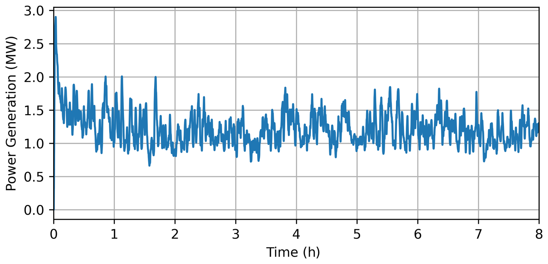
Figure B1 Time trace of power generation for the furthest right turbine in the center row. TI_1.0 atmospheric conditions. Moving/Ocean simulations.

The streamwise projection function is

$$\begin{array}{}\text{(B23)}& S_{\mathrm{S}}\left(x\right)=\left\{\begin{array}{ll}{\left(\mathrm{1}-{\left(\frac{x}{x_R}\right)}^{\mathrm{2}}\right)}^{\mathrm{2}}& \mathrm{if}\mathrm{|}x\mathrm{|}\le x_R\\ \mathrm{0}& \mathrm{otherwise}\end{array}\right.\end{array}$$

which enforces a decay from the projected disk centerline in the streamwise direction to reduce the discontinuity of thrust projection. In this case, x_R=5Δx to enforce a streamwise decay over five cells in each streamwise direction from the disk center.

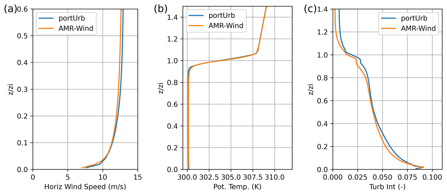
Figure B2 Domain-averaged profiles over $t\in \left[\mathrm{15}\mathrm{000},\mathrm{20}\mathrm{000}\right]$ s. TI stands for turbulence intensity. z_i=800 m is the boundary layer height; (a) $\sqrt{u^{\mathrm{2}}+v^{\mathrm{2}}}$, (b) θ, (c) TI.

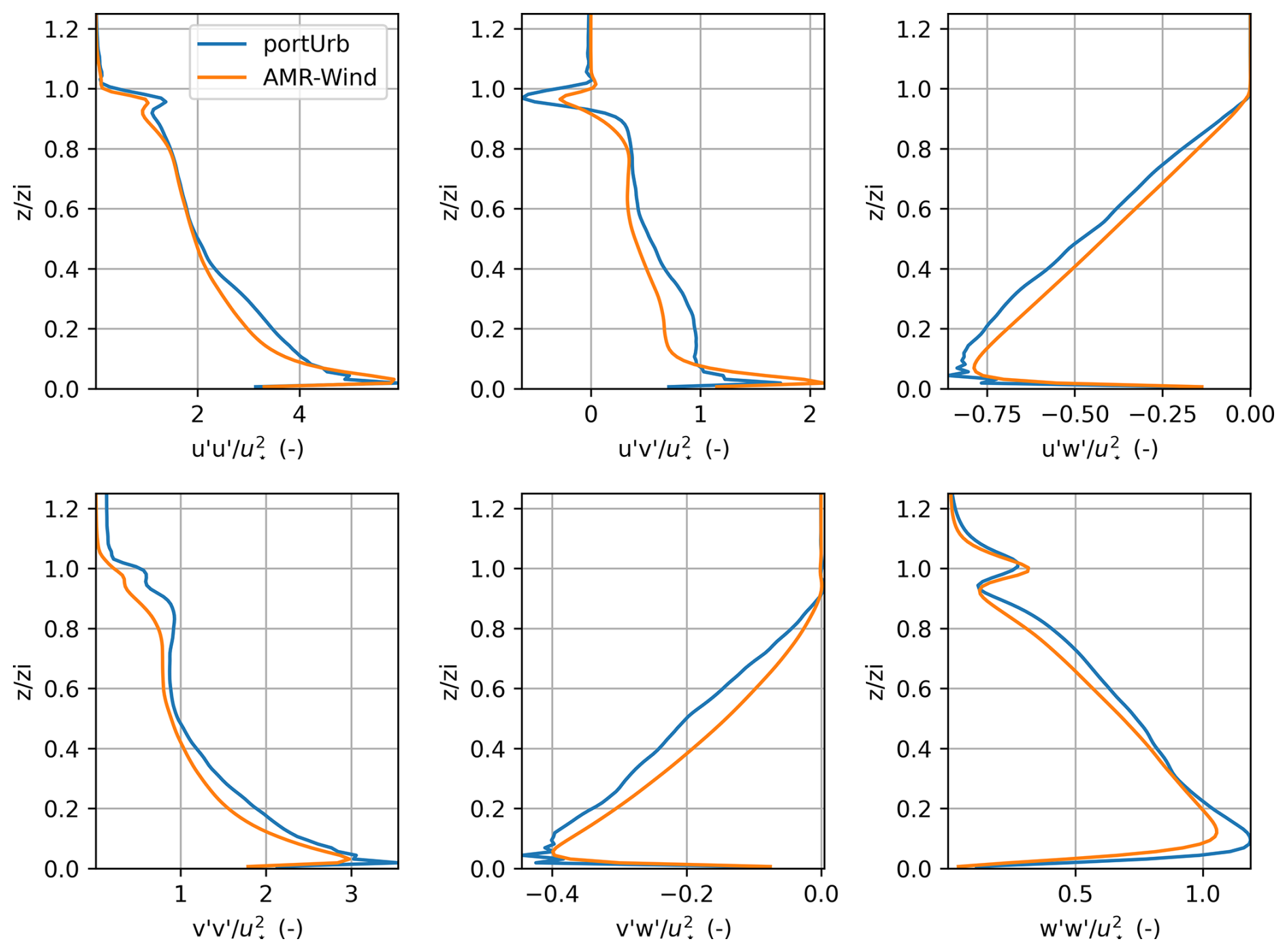
Figure B3 Resolved turbulent velocity correlations. Perturbations are computed as the deviation from the mean column, and correlations are averaged over multiple snapshots within $t\in \left[\mathrm{15}\mathrm{000},\mathrm{20}\mathrm{000}\right]$ s. z_i=800 m is the boundary layer height.

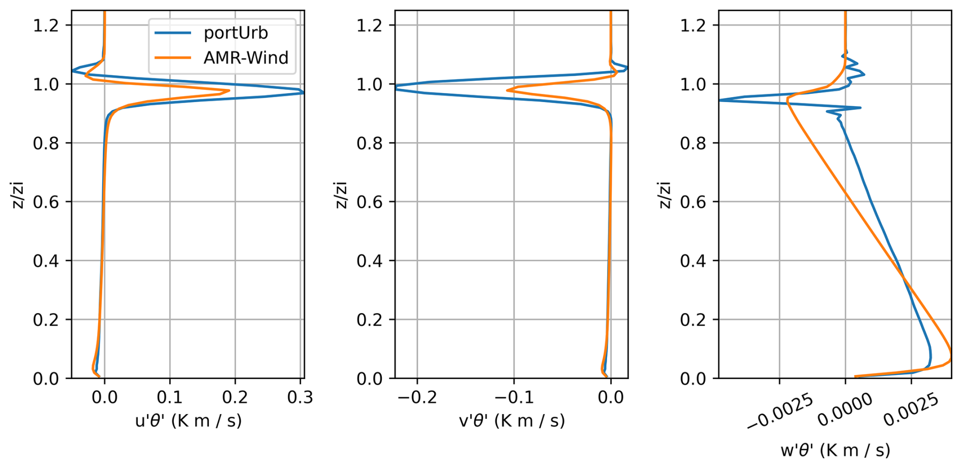
Figure B4 Resolved turbulent temperature correlations. Perturbations are computed as the deviation from the mean column, and correlations are averaged over multiple snapshots within $t\in \left[\mathrm{15}\mathrm{000},\mathrm{20}\mathrm{000}\right]$ s. z_i=800 m is the boundary layer height.

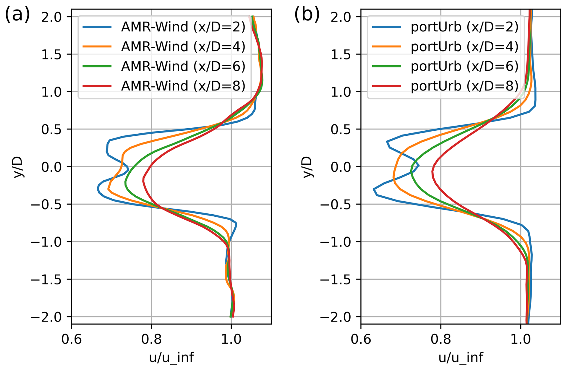
Figure B5 Hub-height (z=90 m) horizontal velocity divided by inflow wind speed (11.4 m s⁻¹) in the y direction at 2, 4, 6, and 8 turbine diameters downstream of the turbine for $t\in \left[\mathrm{15}\mathrm{000},\mathrm{20}\mathrm{000}\right]$ s along the wake direction (30°); (a) AMR-Wind, (b) protUrb.

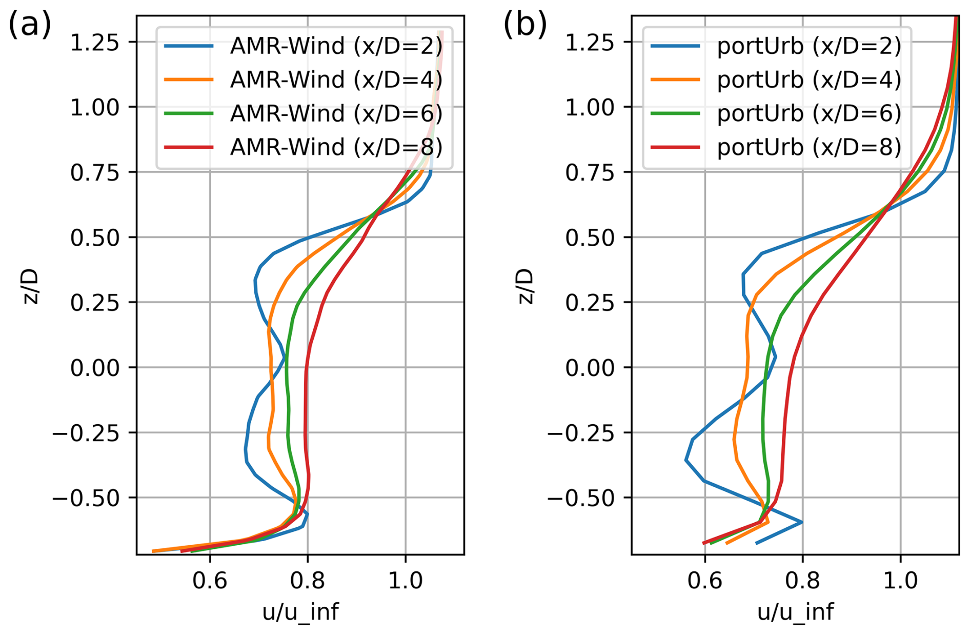
Figure B6 Horizontal velocity divided by inflow wind speed (11.4 m s⁻¹) in the z direction at the turbine center x=1800 m at 2, 4, 6, and 8 turbine diameters downstream of the turbine for $t\in \left[\mathrm{15}\mathrm{000},\mathrm{20}\mathrm{000}\right]$ s along the wake direction (30°); (a) AMR-Wind, (b) portUrb.

Once these weights are computed, a weighted sum using these weights provides the integration of a quantity such as wind velocity over the entire disk.

To summarize:

• Over the domain $\left[-x_R,x_R\right]\times \left[-\frac{D_{\mathrm{T}}}{\mathrm{2}},\frac{D_{\mathrm{T}}}{\mathrm{2}}\right]\times \left[-\frac{D_{\mathrm{T}}}{\mathrm{2}},\frac{D_{\mathrm{T}}}{\mathrm{2}}\right]$ in the x, y, and z directions, evenly create sample points: $\left(x_{\mathrm{initial}},y_{\mathrm{initial}},z_{\mathrm{initial}}\right)$

• Initialize all cell weights to zero: $w_{ijk}^{\star }=\mathrm{0}$.

• For each sample point:

  • a.

    Compute the rotated and translated location $\left(x_p,y_p,z_p\right)$ for the sample point using Eq. (B21).

  • b.

    Locate the cell, C_ijk, in which the point $\left(x_p,y_p,z_p\right)$ is located.

  • c.

    Atomically add the product of the thrust shape and streamwise projection functions to the weights in cell C_ijk: $w_{ijk}^{\star }=w_{ijk}^{\star }+S_{\mathrm{P}}\left(x_{\mathrm{initial}}\right)S_{\mathrm{T}}\left(r_{yz,\mathrm{initial}}\right)$.

    • •

      “Atomically” is an algorithmic term to denote that when parallelizing over sample points (operating on each simultaneously), the sum and update should be performed in its entirety without any other operation accessing (read or write) cell C_ijk's memory. This is to avoid data races.

• Compute the sum of $w_{ijk}^{\star }$ over all cells.

• Divide each weight by the total sum: $w_{ijk}=w_{ijk}^{\star }/{\sum }_{ijk}{w}_{ijk}^{\star }$.

• For any set of cell averages of a quantity ${\stackrel{\mathrm{‾}}{q}}_{ijk}$, compute the disk-integration of that quantity with the sum

  $$\begin{array}{}\text{(B24)}& q_{\mathrm{disk}}=\sum _{ijk}{\stackrel{\mathrm{‾}}{q}}_{ijk}{w}_{ijk}.\end{array}$$

B3 Verification of stationarity for LES-turbine power generation

The time trace of power is plotted in Fig. B1 over the 8 h of simulation for the furthest right turbine in the center row to demonstrate that the simulation has reached an equilibrium state in terms of power production before the $t\in [\mathrm{4},\mathrm{8}]$ h time averaging.

B4 Verification with neutral AWAKEN experiment

The LES code has been validated against standard neutral and convective boundary layer results. Here, it is validated against the AMR-Wind (Kuhn et al., 2025; Brazell et al., 2021) results for a modestly convective boundary layer test case for both turbulent boundary layer results and turbine wake results for the NREL 5 MW turbine used in this study. To initialize, potential temperatures are linearly interpolated between values of 300, 300, 308, and 311.45 K at heights of 0, 750, 850, and 2000 m, respectively. The u and v winds are initialized with a log law setting u=9.873 m s⁻¹ and v=5.7 m s⁻¹ at hub height (90 m), and vertical velocity is initialized to zero. AMR-Wind uses incompressible equations with a Boussinesq buoyancy term with a density of 1 kg m⁻³ throughout; and portUrb uses non-hydrostatic, compressible equations with the surface pressure set to enforce a surface density of 1 kg m⁻³ at a surface temperature of 300 K. Both models perturb the lowest 50 m of the domain with random potential temperature perturbations and use transverse four-period sine waves for u and v velocity in the lowest 100 m.

Coriolis is active with a latitude of 40° N. Surface roughness is set to z₀=0.01 m. The domain is $\mathrm{5.12}\times \mathrm{5.12}\times \mathrm{1.92}$ km in the x, y, and z directions, respectively. A uniform grid spacing of 10 m is used for portUrb, while AMR-Wind has multiple grids that reach 2.5 m grid spacing around the turbine with 10 m grid spacing at the coarsest level. Both models use pressure gradient forcing to force a hub-height horizontal average wind speed of (9.873,5.7) m s⁻¹ for the horizontal velocity vector. That pressure gradient forcing is calculated in the turbulent precursor and then used in both the precursor and primary turbine simulation. The precursor and turbine simulations are run for 20 000 model seconds, the first 15 000 s used as spin-up and the last 5000 s as the performance period. The average pressure gradient forcing over $t\in \left[\mathrm{14}\mathrm{000},\mathrm{15}\mathrm{000}\right]$ s is used throughout the performance period in the main turbine simulation. The turbine is placed at 1800 m into the domain in the x and y directions. A small surface heat flux of 0.005 K m s⁻¹ is added to the surface to create a modestly convective boundary layer.

Figure B2 plots the domain-averaged column of horizontal velocity, potential temperature, and turbulence intensity averaged in time over $t\in \left[\mathrm{15}\mathrm{000},\mathrm{20}\mathrm{000}\right]$ s for AMR-Wind and portUrb. The profiles are quite similar, with portUrb carrying a bit more wind speed and turbulence intensity throughout the boundary layer. Figure B3 plots resolved turbulent velocity correlations averaged over $t\in \left[\mathrm{15}\mathrm{000},\mathrm{20}\mathrm{000}\right]$ s for AMR-Wind and portUrb. The magnitudes and shapes of the profiles are very similar, with portUrb exhibiting some oscillations at the surface peak and at times larger features at the top of the boundary layer. Figure B4 plots resolved turbulent temperature-velocity correlations averaged over the same time range. The $u^{\prime }{\mathit{\theta }}^{\prime }$ and $v^{\prime }{\mathit{\theta }}^{\prime }$ profiles are similar with portUrb exhibiting stronger features at the top of the boundary layer. The $w^{\prime }{\mathit{\theta }}^{\prime }$ profile shows more differences, which is somewhat unsurprising, given the large differences in the buoyancy term. portUrb uses a non-hydrostatic and compressible discretization, where temperature perturbations propagate into density perturbations through acoustics, and the buoyancy term uses density perturbations to determine buoyant forcing. AMR-Wind is incompressible and uses a fixed Boussinesq buoyancy term based on deviations from background temperature (fixed at T₀=300 K throughout the simulation).

Figure B5 plots the turbine wakes at hub height (z=90 m) as a function of y location averaged over $t\in \left[\mathrm{15}\mathrm{000},\mathrm{20}\mathrm{000}\right]$ for portUrb and AMR-Wind at 2, 4, 6, and 8 turbine diameters downstream of the turbine – along the direction of the wake, which is 30°. Both exhibit very similar features and magnitudes, although portUrb is running at 4× larger grid spacing. Both show the asymmetrical profile due to swirl, and both show very similar wake recovery downstream. There are some larger differences in Fig. B6, which plots wakes at the same distances downstream as a function of z location at the hub center, following the wake direction of 30°. The wakes are quite similar higher up, but nearer to the surface, portUrb has a stronger wake deficit – likely due to the coarser grid spacing, leading to surface friction being less separated from the turbine wake.

In summary, despite being formulated quite differently as a model, portUrb replicates the salient features of both the boundary layer turbulence, and the turbine wake deficit shape and magnitude compared to AMR-Wind.