Airborne measurements for investigating offshore wind farm wakes and modifications of sea state – benefits and limitations

In the framework of the two large wind energy research projects WIPAFF and X-Wakes, crewed airborne measurements have been performed in and around wind farm clusters of the German Bight to investigate offshore wind farm wakes and associated sea state modifications. These flights offer high spatial flexibility. Routes can be adapted in real time to wind direction, stability, wake extent, and features of interest, providing complementary coverage to fixed ground-based instruments and remote sensing systems. Aircraft-based observations achieve high vertical resolution on the order of several centimetres and allow simultaneous measurements of wind speed, turbulence, thermodynamic variables, air–sea fluxes, and sea surface characteristics. This enables a detailed description of wake structure, wake recovery, and the influence of atmospheric stability, as well as the interaction of multiple wakes across scales of tens to hundreds of kilometres. Airborne measurements also provide a direct link between atmospheric changes and sea-surface modifications, such as altered roughness or wave patterns, and supply valuable data for evaluating simulations and improving parameterizations used in wind farm modelling. When combined with satellite remote sensing, they help bridge the gap between high-resolution local observations and large-area coverage. A central limitation of aircraft campaigns is their restricted temporal coverage. Flights are episodic and sample evolving atmospheric conditions over finite time periods, which complicates the comparison with satellite snapshots and limits the ability to derive long-term statistics. Small wind farm effects that are on the order of the natural variability in the background flow are easily masked by natural variability in the marine boundary layer. Therefore, the global blockage effect is difficult to isolate using aircraft data alone. Overall, aircraft-based observations offer unique strengths when integrated with other measurement systems and modelling tools, despite inherent temporal constraints. This article summarizes which effects benefit from the analysis of airborne data sets and shows examples where they helped to improve the understanding of the interaction of wind farms, atmosphere, and sea state significantly.

1 Introduction

The transformation of energy towards renewable resources requires the worldwide installation of large capacities of wind power. Offshore wind farm clusters play a key role in the increase in the share of renewables, as offshore sites typically offer more reliable and stronger wind conditions than onshore locations (Veers et al., 2019). The globally installed offshore wind capacity is expected to increase from 75.2 GW (as of 2024) to 380 GW by 2030 and to 2000 GW by 2050. In Germany, an installation of a total capacity of 30 GW is planned by 2030 and even 70 GW by 2045 (Williams et al., 2025).

It is a physical fact that offshore wind farms are associated with wind farm wakes, but the large extent of wakes for offshore environments has only recently been explored (Platis et al., 2018). Wakes are defined as a region of reduced wind speed and increased turbulence downwind (e.g. Schneemann et al., 2020). Airborne measurements have provided key data to quantify wake extent and wind speed recovery under different atmospheric conditions (Platis et al., 2020; Cañadillas et al., 2020).

With the strong future expansion in offshore installations of wind capacities, an increasing area will be influenced by wind farm wakes (Pryor and Barthelmie, 2021; Akhtar et al., 2021; Bodini et al., 2021). Especially wake impacts on downstream farms have become increasingly important in the overall planning of offshore farms in recent years (Ouro et al., 2025). The installation and operation of large offshore wind farms have environmental and technological consequences (Bailey et al., 2014; Windt et al., 2024), as well as socially relevant aspects, like a different visual appearance (Ladenburg, 2009), which is not an issue because of the far-offshore placement in the German Bight. Large wind farms can modify the atmospheric boundary layer, cloudiness, and precipitation (Akhtar et al., 2022). For the additional implementation of offshore wind farms, the overall mutual impacts of and on the existing wind farms and their wakes have to be taken into account. This refers to reduced available wind resources as well as increased downstream turbulence intensity, which has an impact on fatigue loadings within wind farms (Sathe et al., 2012; Lee et al., 2013; Vera-Tudela and Kühn, 2017), but only very limited impact for far-downstream cluster wakes (Anantharaman et al., 2025). Further, the impacts on sea state (Bärfuss et al., 2021; Schmitt et al., 2026), ocean stratification (Lian et al., 2022; Christiansen et al., 2022), and ocean circulation (Broström, 2008) are supposed to increase, with secondary effects for the ecosystem (Daewel et al., 2022). As the electrical grid and feed-in planning relies on an increasing share of the highly flexible resource of wind power (Drew et al., 2015), it is of crucial importance to be able to predict the power output with high reliability on the timescale of days and hours. Knowledge of wind resources is also essential for the financing of wind farm projects (Mora et al., 2019). Further, with an increasing impact of wakes on neighbouring wind farms, resulting in reduced energy output (Lundquist et al., 2019), international planning gains importance (Finserås et al., 2024). Therefore, characterizing wind farm wakes is of large importance. An enhanced understanding is required to develop suitable parameterizations for wind farm models of different complexity, from fast engineering models (Bastankhah and Porté-Agel, 2014; Nygaard et al., 2020) to mesoscale weather models (Fitch et al., 2012; Vollmer et al., 2024). In contrast, large-eddy simulations (LESs; Wu and Porté-Agel, 2011; Dörenkämper et al., 2015) fully resolve the flow around and through turbines, assuming actuator discs to be a sufficiently good representation. At the same time, the deployment of LES for resource assessment is limited due to the large computational costs. As mentioned in several review articles, the lack of offshore data characterizing the marine atmospheric boundary layer is a major drawback for improving understanding and simulations (Veers et al., 2019; Shaw et al., 2022).

The motivation to perform airborne measurements to characterize the properties of offshore wind farm wakes was provided in 2012 by radar satellite images, where a modification of the water surface downstream of wind farm areas was evident (Christiansen and Hasager, 2005), and the first simulations suggested a much higher wind speed deficit and long-reaching wakes under stable atmospheric conditions (Fitch et al., 2012; Abkar et al., 2016). The first project for airborne in situ measurements in the wake of offshore wind farms, WIPAFF, was finally funded in 2015 (Emeis et al., 2016). This first project proved the existence of far-reaching wind farm wakes extending several tens of kilometres under stable atmospheric conditions and provided a first idea of the impact of wakes on the sea surface. Another proposal was initiated in 2017, and finally the project called X-Wakes was funded with an extended consortium in 2019.

The article presents progress in the field of offshore wind farm wake research based on measurements with crewed aircraft. To the authors' knowledge, these are so far the only airborne observations worldwide with the purpose to study the wakes of entire wind farms. The article summarizes results that are already published and adds new aspects which have not yet been published so far. Such new material includes

• the direct comparison of almost-simultaneous airborne in situ measurements and satellite-derived wind field in the wake of wind farms (Sect. 3.1)

• a study of changes in sea surface properties (Sect. 3.6)

• limitations in identifying the global blockage effect by airborne measurements (Sect. 3.7).

The article is structured as follows: Sect. 2 introduces the methodology of airborne in situ measurements of offshore wind farm wakes. Section 3 presents an overview of several phenomena associated with offshore wind farm wakes that were investigated with airborne measurements: Sect. 3.1 provides the improvement of wake characterization by airborne observations. Section 3.2 demonstrates the interaction of wakes of different wind farms. Section 3.3 shows the modification of latent heat fluxes in wakes, which may be responsible for local cloud formation at wind farms. Section 3.4 provides an overview of coastal effects, which is the modification of the wind field across the coast line. Section 3.5 presents airborne data as used for model validation. Section 3.6 demonstrates the link of wind farm wakes to modified sea surface properties. Section 3.7 illustrates the limits of airborne measurements, which is the observation of small effects due to the limited observation time and constraints in flight patterns close to wind farms, with the example of the global blockage effect. Finally, Sect. 4 summarizes the results in the conclusions.

2 Methodology of airborne in situ wake measurements

The airborne offshore wind farm wake measurements were mainly performed with the research aircraft Dornier 128 with call sign D-IBUF of TU Braunschweig (Corsmeier et al., 2001; Lampert et al., 2020), and in addition several flights were done in parallel with the research aircraft Cessna F406 with call sign D-ILAB of TU Braunschweig (Lampert et al., 2024). The typical air speed was around 65 m s⁻¹.

The meteorological instrumentation for measuring the high-resolution (100 Hz) wind vector, temperature, and humidity is installed in the nose boom. For the wind vector, this includes a five-hole probe (Rosemount, USA) and sensors for differential and total pressure (Setra, USA) to determine the airflow angles. The position and orientation of the aircraft are determined with a combination of an inertial measurement unit (IMU; different systems for the Dornier 128: iNAV-RQH-1003, iMAR, Germany; for the Cessna F406: iNAT-RQT-4001, iMAR, Germany) and a global navigation satellite system (GNSS; receiver OEM6, NovAtel, Canada). The wind vector can then be derived by subtracting the air speed vector from the ground speed vector. The temperature is measured by two complementary sensors: one with high accuracy but slower response time (102DB1AG, Rosemount, USA) and one with lower accuracy but higher response time (102E4AL, Rosemount, USA). Humidity is measured with three different sensors: a capacitive sensor Humicap H233 (Vaisala, Finland), a dew point mirror TP 3-S (Meteolabor, Switzerland), and a fast but drifting optical sensor (for the Dornier 128: Lyman-alpha sensor L-6/HMS-2, Buck Research, USA; for the Cessna F406: KH-20, Campbell Scientific, USA). The different sensors are combined by advanced data fusion techniques, like complementary filtering and Kalman filters, to gain data of enhanced quality and reduced uncertainties, as described e.g. in Bärfuss et al. (2018). This is generally of high importance for improving airborne measurements of the wind speed (e.g. Cayon et al., 2025).

Additional instruments for measuring surface temperature, sea state, and solar and terrestrial radiation are installed in the aircraft cabin: an infrared radiation thermometer (KT15.82D in the Dornier 128 and KT19.85 in the Cessna F406, Heimann, now Heitronics, Germany), a laser scanner VZ-1000 (Riegl, Austria, only for the Dornier 128), two pyranometers for measuring upward and downward solar irradiance (CMP22, Kipp and Zonen, the Netherlands), and two pyrgeometers for measuring upward and downward terrestrial irradiance (CGR4, Kipp and Zonen, the Netherlands). The radiation sensors are only available for the Cessna F406. More details on the sensors and the accuracies are provided in Lampert et al. (2020) and Lampert et al. (2024).

The measurements for investigating wind farm wakes were performed at hub height crossing the wind farm wake perpendicular to the wind direction at different downstream distances. Based on these in situ measurements, vertical mixing in the atmospheric boundary layer is identified by fluctuations in the vertical component of the wind speed vector. This allows the calculation of turbulent kinetic energy, momentum fluxes, and heat fluxes. In addition, ascending and descending flight tracks from very low altitudes (15 m) to the free troposphere (1 km) were integrated in the flight pattern regularly to determine atmospheric stability, (almost-)vertical profiles of the wind vector, and the temporal and spatial variability in the wind field. Each horizontal flight leg across the wake typically had a distance of 40 km in order to capture also the undisturbed flow to both sides and took around 10 min. The ascent and descent took around 2 min between the minimum and the maximum flight altitude, resulting in a horizontal displacement of around 8 km. The upstream conditions were also probed. For investigating wake interactions, flights across wake areas were done between and downstream of different wind farms. The overall duration of one flight was around 4 h and included the ferry from the airport with jigsaw patterns of vertical profiles to investigate the spatial development of the atmospheric boundary layer (ABL); then the pattern to sample the wake, including the vertical profiles in between the legs; and the ferry back. Other flight patterns were dedicated to changes in meteorological parameters above the wind farms, to the global blockage effect with upstream measurements, and to modifications of the atmospheric boundary layer induced by the influence of the coast. Detailed explanations of the aircraft, the sensors, and the different flight patterns are provided in Lampert et al. (2020) and Lampert et al. (2024).

In addition to continuous measurements at fixed locations, airborne measurements provide the opportunity to determine the spatial variability and a complementary data set for intensive observation periods. This allows the representativeness of continuous profile measurements to be studied, like at the meteorological masts FINO1 (e.g. Wagner et al., 2019; Spangehl et al., 2023) and FINO3 (e.g. Peña et al., 2015; Olsen et al., 2022) for the German Bight (Platis et al., 2021a). Further, lidar profile measurements at one location can be embedded in the context of spatial variability in the wind field by airborne observations (Cañadillas et al., 2022). Airborne measurements can also be used to characterize the sensitivity of stability definitions to the height interval of local measurements, e.g. air temperature at only two heights compared to high-resolution vertical profiles acquired by aircraft (Platis et al., 2021a). The analysis of airborne measurements has to take into account the synoptic spatial and temporal variability in the wind field. Stationary conditions cannot be assumed over the 4 h time period of a research flight. Therefore, it turned out to be not possible to use the upstream wind field as a reference for the downstream modifications, as planned originally. Instead, the wind speed in the wake area was compared to the wind speed in the undisturbed area next to the wind farm wake area for each of the flight legs (Cañadillas et al., 2020). Spatial gradients of the wind field across the wake area were frequently present as well (Platis et al., 2018).

3 Airborne observations of offshore wind farm wakes and associated phenomena

In the following, different aspects of offshore wind farm wakes are considered from the perspective of airborne measurements, as published by Bärfuss et al. (2019) and Rausch et al. (2023a). As the wind speed in the published data sets shows a small cross-correlation regarding the wind impact angle on the flight path (angle between wind direction and flight direction) – likely caused by pressure transducers with temperature and temperature gradient effects out of the valid ranges – the wind speed data were corrected by the assumption of a constant aircraft sideslip angle error for the analyses in Sects. 3.1 and 3.2, with subsequent median filtering over a time window of 30 s. The systematic wind speed correction was derived by analytically estimating wind speed perturbation caused by a static installation offset and a small angle-of-sideslip error using a first-order linearization of the wind derivation equations (see e.g. Bärfuss et al., 2023). Assuming an absolute error of 0.3° on the angle of sideslip and a measurement speed of 65 m s⁻¹, the wind speed error in the 100 Hz data is ±0.35 m s⁻¹ on flight legs perpendicular to the prevailing wind direction.

3.1 Wind farm wake characterization

The wind farm wakes were characterized by flying meander patterns, i.e. individual flight tracks, called legs, oriented perpendicular to the prevailing wind direction. Typically, in the framework of the campaigns conducted in the projects WIPAFF and X-Wakes, the transects through the wake region were spaced with a horizontal distance of 10 km. The closest flight leg was at a distance of 500 m downstream of the wind farm due to flight permissions. For neutral and unstable conditions, the distance between the flight legs was reduced. In this way, the horizontal extent and the wind speed recovery of wind farm wakes were quantified. Under neutral conditions, wakes extend several kilometres downstream (Cañadillas et al., 2020), under stable atmospheric conditions at least several tens of kilometres (Platis et al., 2018). The recovery of the wind speed can be approximated by an exponential function, with a typical recovery up to 95 % of the undisturbed wind speed after a downstream distance of around 55 km for stable and 20 km for unstable conditions (Cañadillas et al., 2020), with high variability (Foreman et al., 2025). This recovery, in particular for stable conditions, is significantly slower than usually assumed in industry models (Cañadillas et al., 2020; Platis et al., 2020) but on the order of magnitude predicted by simple analytical stability-dependent wind farm models such as EFFWAKE (Emeis, 2010, 2022). The wake length (Platis et al., 2020) and also the initial wind speed deficit directly downwind of the wind farms (Platis et al., 2021a) strongly depend on atmospheric stability, but also other parameters, like wind farm geometry and density, seem to have a major influence. Downstream of wind farms, vertical mixing is enhanced at the altitude range of the rotor blades. This vertical mixing can result in micrometeorological changes: either warming or cooling of the air at hub height and either drying or moistening of the downstream atmosphere, which depends on the altitude of the temperature inversion and the moisture distribution with height (Siedersleben et al., 2018b). The airborne measurements show that directly above the wind farms, turbulence is strongly increased (Siedersleben et al., 2020).

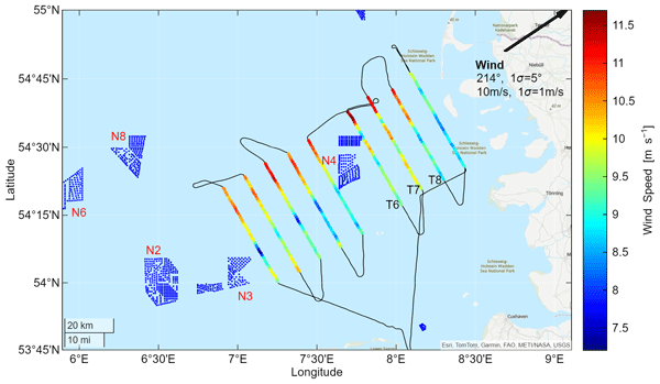
Although the methods of airborne in situ measurements of wakes and satellite-borne remote sensing observations based on synthetic aperture radar (SAR) are highly different and sample on other spatial and temporal scales, the quantification of wakes based on the regular SAR overpasses is important for monitoring and is compared to almost-simultaneous airborne measurements in the following. Figure 1 shows the wind speed at 10 m height derived from SAR imagery. The radar data were obtained on 11 September 2021 at 17:17 UTC, and the 10 m wind speed with a horizontal resolution of 300 m was derived from the normalized radar cross-section (NRCS) using a C-band geophysical model function CMOD5N (Hersbach et al., 2007; Verhoef et al., 2017; Djath et al., 2018). For a potential explanation of the higher wind speed values close to the coast, the reader is referred to Sect. 3.4. Figure 2 displays an almost temporally overlapping measurement flight carried out in the same area between 12:51–17:13 UTC. The SAR snapshot provides a quasi-synoptic view of the near-surface wind field at the end of the flight period, while the aircraft sampled the same flow along several transects at hub height and in vertical profiles. Downstream of the wind farm cluster N4, both observations capture a decrease in the wind speed for the individual wind farms Amrumbank West, Nordsee Ost, and Meerwind Süd-Ost (from north to south) and a speed-up in the so-called “Kaskasi gap” between Amrumbank West and Nordsee Ost, where the wind farm Kaskasi was built after the flights were conducted. For a more detailed comparison, Fig. 3 shows the wind speed measured along three horizontal transects (T6, T7, and T8).

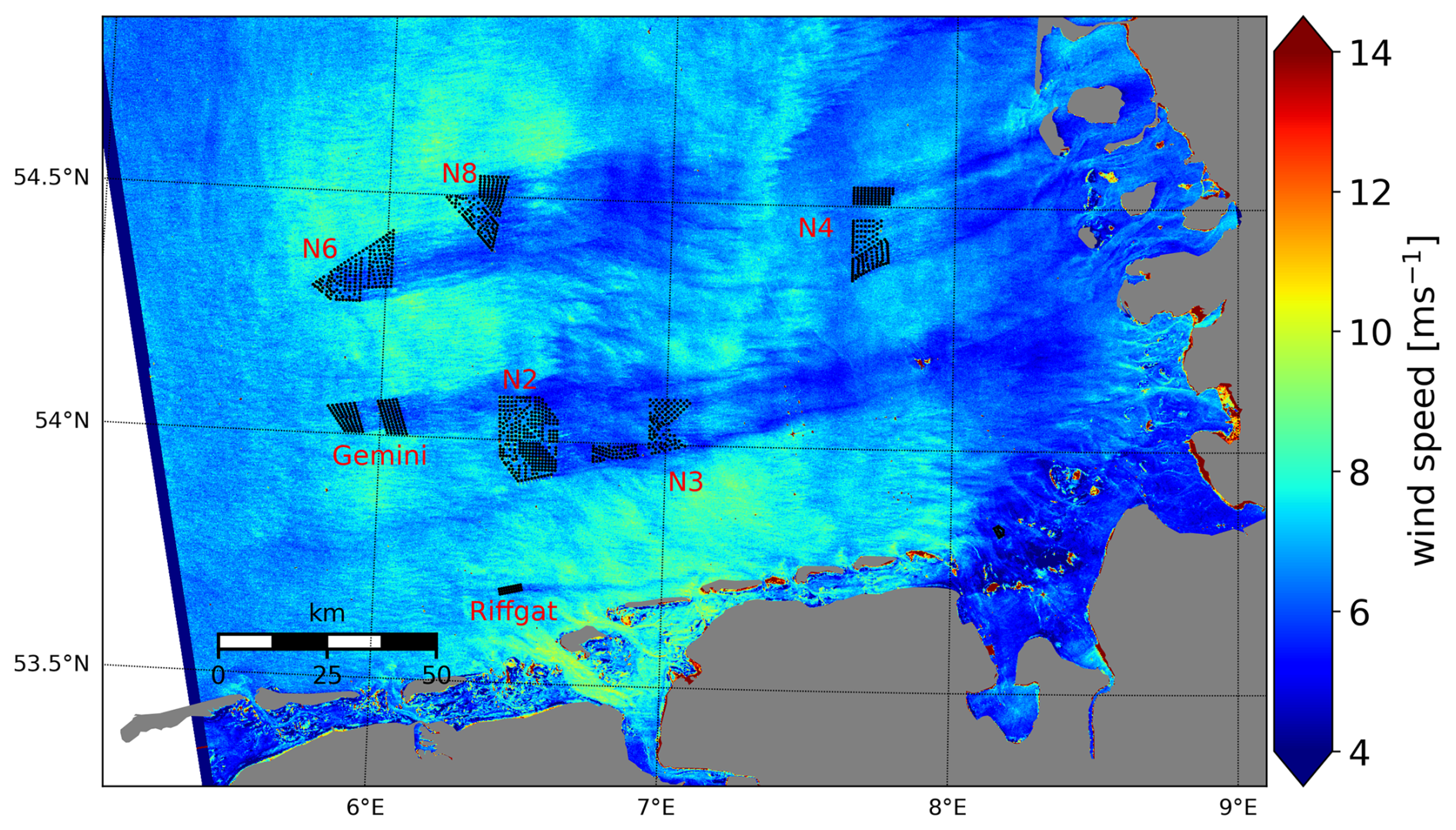
Figure 1 The 10 m wind speed derived from Sentinel-1A SAR (contains modified Copernicus Sentinel data (2021)) data acquired on 11 September 2021 at 17:17 UTC. Black dots represent wind turbines; names of wind farms and clusters are labelled in red. The map was generated by Bughsin Djath using Python, Matplotlib, and Basemap.

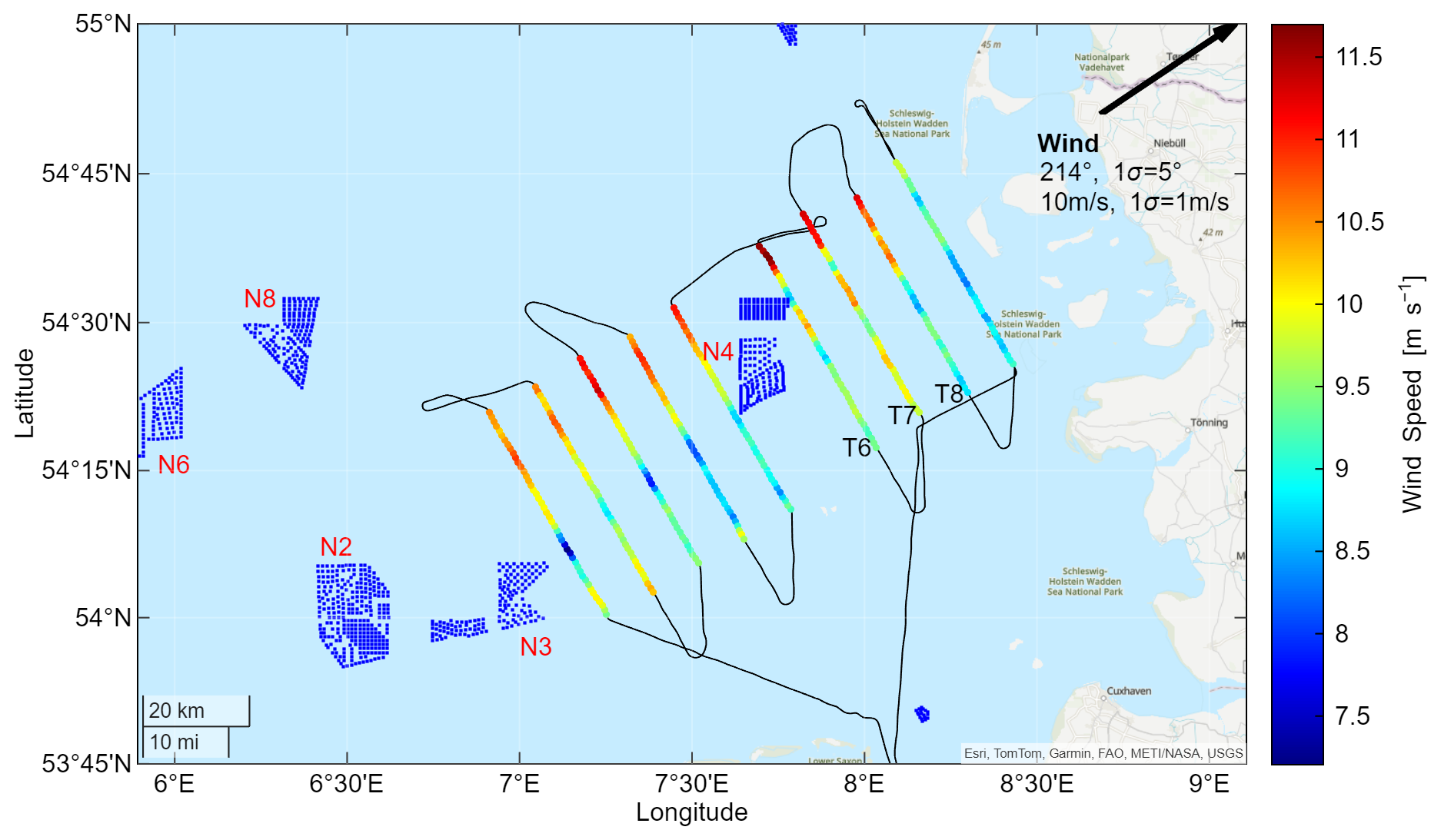
Figure 2 In situ wind speed measured on 11 September 2021 by the research aircraft D-IBUF from 12:51 UTC to 17:13 UTC in the lee of wind farm clusters N2 and N3 for the south-westerly wind direction. Blue dots represent the individual wind turbines; black lines represent the flight path of the aircraft. Wind speed measurements along the flight path perpendicular to the main wind direction are colour-coded and plotted for every 15 s, corresponding to a displayed horizontal resolution of around 1 km. One flight leg of around 45 km length requires a flight time of around 12 min. The indicated transects through the wakes T6, T7, and T8 are used for direct comparison with satellite data in Fig. 3. The arrow indicates the main wind direction. The variability in the wind field during the measurement flight is illustrated by the standard deviations of wind speed and wind direction. Esri, TomTom, Garmin, FAO, METI/NASA, USGS | Powered by Esri.

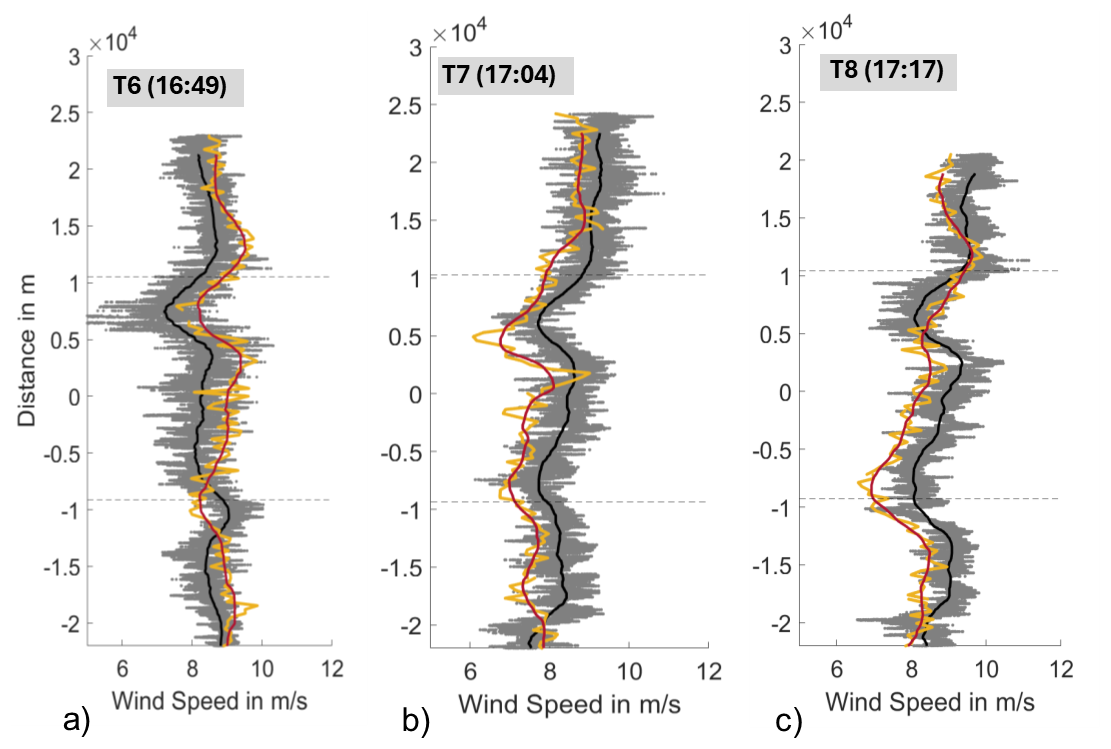
Figure 3 Comparison of airborne wind measurements with the research aircraft D-IBUF at hub height (running mean, black) showing substantial small-scale variability (grey shading) with collocated SAR-derived wind speed (red) and variability (yellow) on 11 September 2021. The SAR wind speed was extrapolated from an altitude of 10 m to hub height using stability information obtained from the flight. The gaps in the SAR-derived data are caused by quality filtering of unrealistic SAR wind speed values due to turbine-related SAR artefacts close to the wind farm Amrumbank West. Panels (a–c) correspond to different sampling times (in UTC) and transects called T6, T7, and T8 of the flight data. One flight leg of around 45 km length requires a flight time of around 12 min.

Satellite-based estimations typically derive the wind speed at hub height in several steps indirectly from the height of the capillary waves at the surface, which are an indicator for the wind speed and roughness at the surface. From those, the 10 m wind speed was derived first. Then the SAR-derived 10 m wind speed was extrapolated to hub height using stability information obtained from the airborne profiles. One should note that extrapolating from SAR-derived 10 m wind speed towards hub height introduces uncertainty related to atmospheric stability, surface roughness, and the vertical wind profile. This uncertainty is reduced here by using stability information from the flight profiles, but the stability functions used in the extrapolation are still idealized (Garrat, 1994).
Airborne in situ measurements along these transects show substantial small-scale variability and enhanced turbulence, whereas the collocated SAR-derived hub-height winds provide smoother fields because of the finite radar footprint and the averaging applied in the retrieval (Djath et al., 2018). Despite the high-frequency fluctuations observed in the airborne data, the SAR-derived wind speed closely follows the mean airborne signal for all transects. Small discrepancies are visible, particularly in regions of enhanced turbulence (e.g. at distances of around 0.5–1.5 km for the transects at 16:49 UTC and 17:04 UTC), but the overall agreement is high in both magnitude and spatial pattern. For transects T6–T8, the SAR-derived and airborne wind speeds show an overall agreement with a root mean square (rms) of 0.8 m s⁻¹ and a correlation coefficient of 0.8. The bias varies between the individual transects (including a change in sign between T6 and T7/T8), indicating that the differences are not systematic across all transects and may depend on local atmospheric boundary layer conditions. The standard deviation of the SAR and airborne wind speed differences is about 0.3 m s⁻¹. The joint analysis highlights the complementarity between airborne and satellite observations in offshore wind farm wake studies. Aircraft-based measurements provide an independent reference at hub height and resolve turbulence and vertical shear on scales that cannot be captured by SAR, thereby supplying essential context for interpreting SAR-derived wake signatures. At the same time, SAR offers an instantaneous, spatially extensive view of the near-surface wind field that cannot be achieved by aircraft alone. Together, these platforms show that SAR-derived wind speed can reliably reproduce the horizontal wind field at hub height when combined with appropriate stability information and can therefore serve as a consistent complement to airborne measurements.

Overall, compared to other wake measurement methods, airborne measurements offer several advantages. These include the ability to directly validate satellite-derived wind speed at hub height. Satellite-based techniques typically derive the wind speed at hub height indirectly, using surface roughness to estimate the wind speed at 10 m and subsequently extrapolating to hub height. Airborne measurements also extend the spatial coverage provided by long-range scanning wind lidar systems, which are typically fixed at a single location and can retrieve wind field data over distances of up to approximately 15 km, depending on atmospheric conditions. The effective range of these systems is influenced by several factors, including aerosol concentration (which influences backscatter strength), atmospheric visibility and humidity (which affect signal attenuation), laser pulse energy and optical design (which influence system sensitivity), and the scanning geometry (as longer path lengths or steeper elevation angles can reduce the signal-to-noise ratio). In contrast, point measurements from fixed installations such as the FINO1 meteorological mast (FINO1, 2025) provide data with high precision and high resolution in time but are limited to single locations where additional measurements are needed to estimate wake strengths.

3.2 Wake interaction

Airborne observations provide the opportunity to focus the measurement strategy on covering overlapping wake effects of multiple wind farms and to confirm numerical simulations of the wind field. The interaction of different wind farm wakes has been investigated by numerical simulations of different complexity (Cañadillas et al., 2020, 2023b; Foreman et al., 2024; Sengers et al., 2024) and by satellite images providing an overview of large scales (Djath et al., 2018). Figure 4 shows airborne measurements which confirm the further reduction in the wind speed downstream of a second wind farm, with the wind speed reduction depending on turbine density and the mode of operation (Cañadillas et al., 2022; zum Berge et al., 2024).

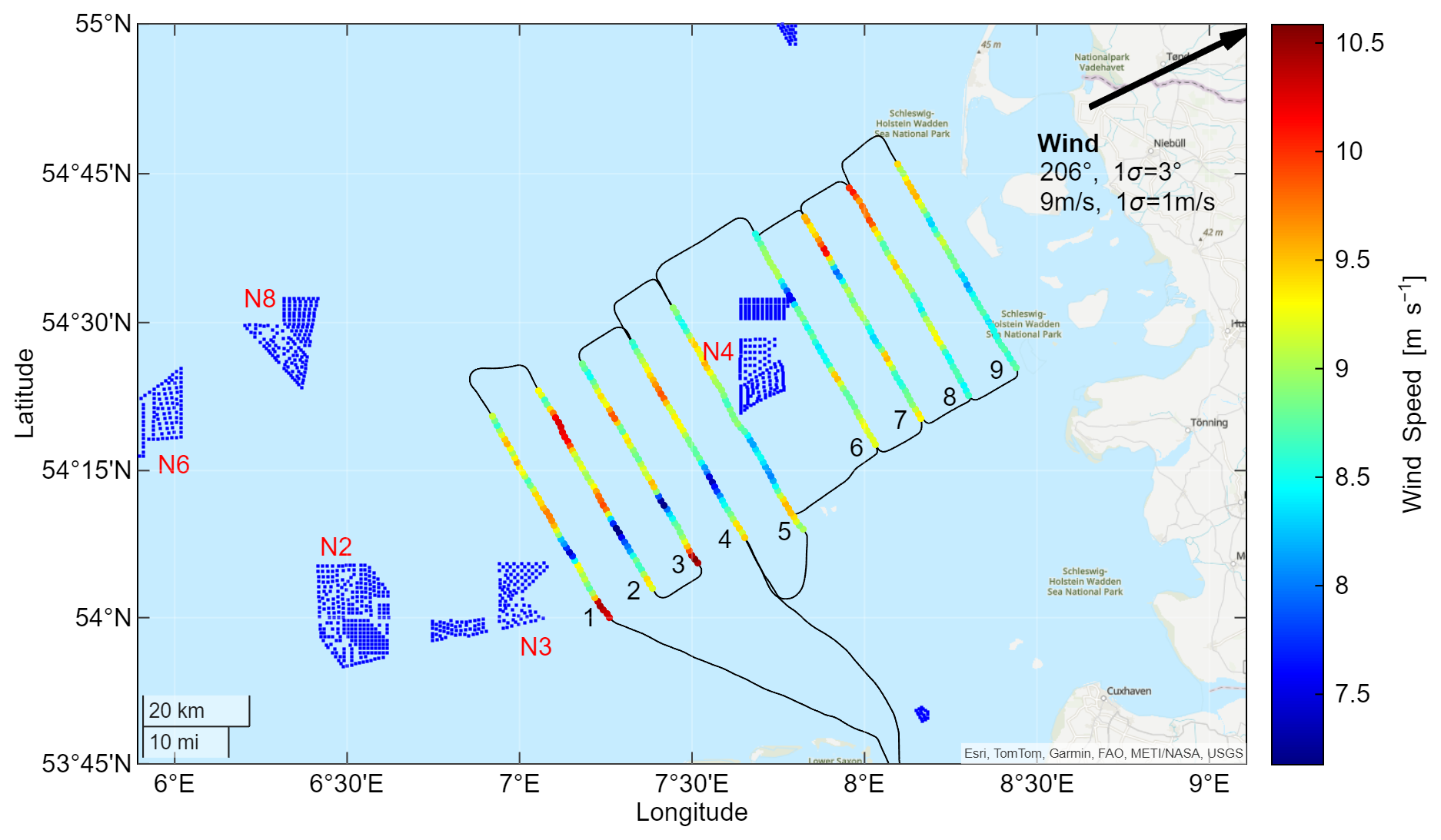
Figure 4 Wind speed measured at hub height in situ by the research aircraft D-IBUF in the lee of wind farm clusters N2 and N3 for the south-westerly wind direction on 27 July 2021. Blue dots represent the wind farm cluster; black lines represent the flight path of the aircraft. Wind speed measurements along the flight path perpendicular to the main wind direction are colour-coded and plotted for every 15 s. One flight leg of around 45 km length requires a flight time of around 12 min. The arrow indicates the main wind direction. The variability in the wind field during the measurement flight is illustrated by the standard deviations of wind speed and wind direction. Esri, TomTom, Garmin, FAO, METI/NASA, USGS | Powered by Esri.

Building on these findings, zum Berge et al. (2024) evaluated both engineering and mesoscale models using the in situ airborne measurements behind large-scale wind farm clusters in the German Bight. The study compared four representative measurement flights with simulations from the Weather Research and Forecasting Model (WRF), developed by the National Center of Atmospheric Research widely used in the wind energy community (Skamarock et al., 2019), including wind farm parameterizations and several engineering wake models implemented in the FOXES software tool (Schmidt et al., 2023). Results showed that engineering models, when properly configured or coupled with mesoscale input, are capable of reproducing wake effects over tens of kilometres, including merged wakes from multiple farms. Particularly the engineering model coupled with WRF (EM-WRF; Fig. 7) – where a heterogeneous, undisturbed WRF background simulation is used as input to initialize each turbine locally, and turbine wakes are propagated as passive scalars along the atmospheric flow streamlines derived from the WRF data (zum Berge et al., 2024) – proved to be most consistent with the airborne observations, especially under stable stratification.

All models (see Fig. 7) showed a reduced accuracy in predicting wake position and strength at distances beyond 30 km from the wind farm cluster. Therefore, accurate inflow conditions and proper atmospheric stability characterization are required to improve the performance of all model results over such large scales. Unlike traditional meteorological masts, which only provide single-point time series, or Doppler lidars, which are limited to a scanning range of about 10 km, in situ airborne measurements allow the full, large-scale cluster wake developments that can extend beyond 50 to 70 km to be captured under stable atmospheric conditions (Platis et al., 2020). By flying meandering patterns perpendicular to the wind direction at hub height across multiple locations, aircraft data uniquely provide high-spatial-resolution cross-sections of the wind field. This makes it possible to simultaneously evaluate wake deficits, lateral wake extent, and merged wake structures from multiple adjacent wind farm clusters across vast horizontal distances.

On the other hand, the results of the model comparison also underline the difficulties of using only one aircraft, lacking simultaneous inflow measurements. Further, the lack of repetition of similar conditions makes it hard to remove or quantify uncertainty based on aircraft measurements.

3.3 Modification of latent heat fluxes

Airborne measurements were able to show that latent heat fluxes increased above and downstream of wind farm clusters across a range of atmospheric stability regimes (Platis et al., 2023). Latent heat fluxes were calculated based on the eddy covariance method, correlating the fluctuations in the vertical wind speed component and the fluctuations in the mixing ratio based on measurements of the Lyman-alpha fast humidity sensor. More details of the averaging method are explained in Platis et al. (2023). Under thermally stable conditions, nearly all flights showed a notable increase in upward latent heat flux above the wind farms, with maximum enhancements reaching +160 W m⁻² relative to background conditions. During near-neutral stratification, the latent heat flux enhancement was generally stronger, with peak values up to +600 W m⁻², although more spatially confined. The data suggest that while the signal is more consistently detectable during stable conditions, it becomes more pronounced under neutral conditions. This is likely due to enhanced vertical mixing induced by the wind farms, which facilitates downward entrainment of drier air into the near-surface layer, enhancing the evaporation potential. The increase in latent heat flux was generally limited to the area above and immediately downstream (up to around 1 km) of the wind farms (Fig. 5), while the associated wakes extended further downwind, indicating different spatial scales of momentum and scalar flux modifications. The distance of the flight trajectory to the wind farms varies due to wind park geometry and wind direction, resulting in visible effects of the latent heat fluxes only for part of the areas indicated as downstream of the wind farms in Fig. 5.

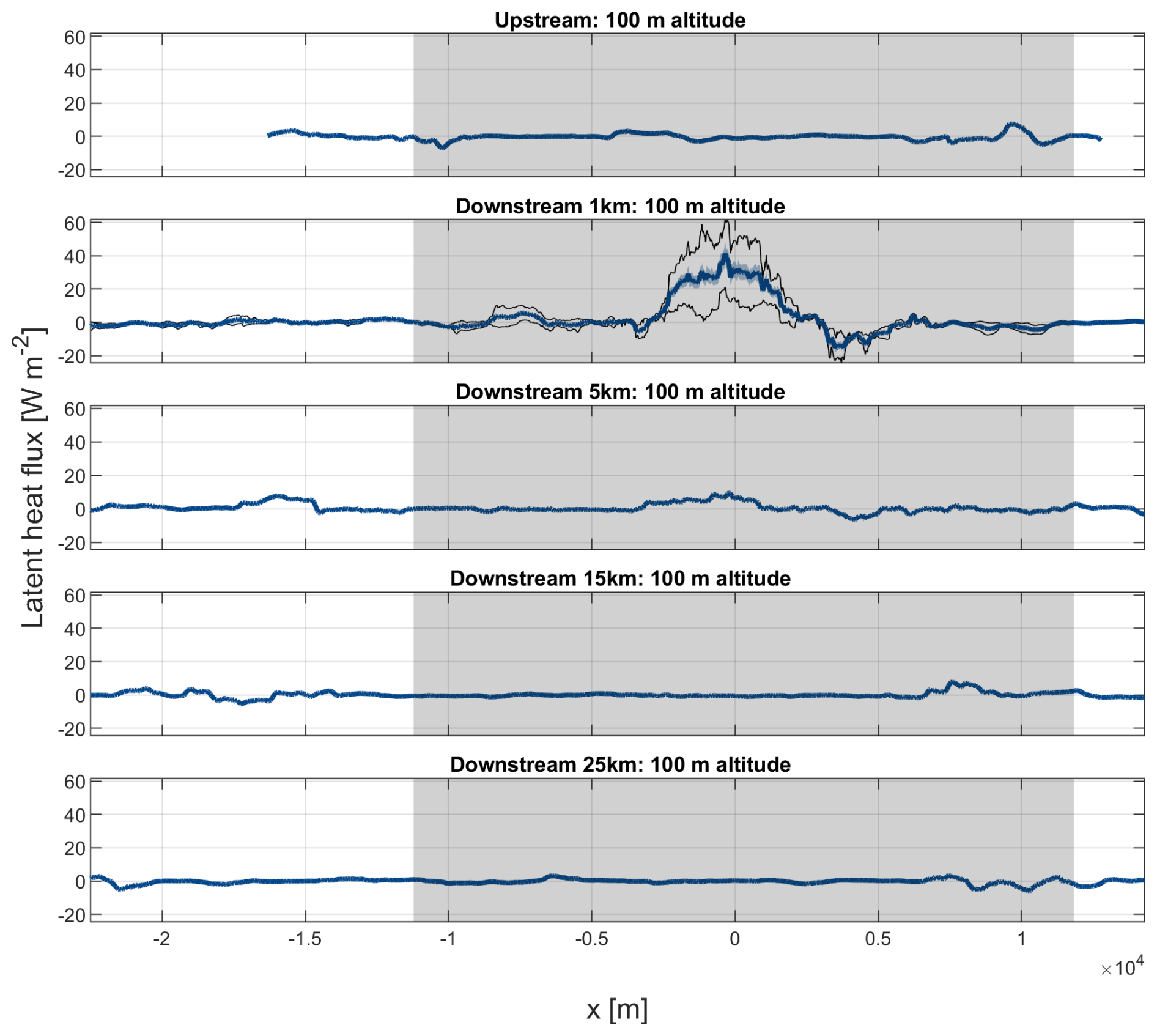
Figure 5 Airborne observations obtained with the research aircraft D-IBUF of the turbulent latent heat flux on 27 May 2017 during a research flight at the Amrumbank West wind farm cluster N4. Measurements were taken upstream and downstream of the cluster under weakly stable thermal stratification, with a capping inversion located at around 800 $\mathrm{m}\mathrm{a}.\mathrm{s}.\mathrm{l}.$. The figure presents the latent heat flux collected along two consecutive flight legs aligned perpendicular to the prevailing wind direction of 130° and flown at hub height (100 m). The blue line represents the averaged latent heat flux across both flight legs, while the grey-shaded area indicates the projected position of the Amrumbank West wind farm along the mean wind direction. The blue-shaded envelope denotes the measurement uncertainty associated with the latent heat flux. The figure has been published in Platis et al. (2023).

However, attributing the observed effects solely to wind farm influence also remains challenging for airborne observations due to varying flight patterns, measurement altitudes, atmospheric background variability, and limitations in a suitable definition for accurately classifying stability (Platis et al., 2021a). Additionally, wind farm characteristics such as turbine layout and density likely play a role in modulating the magnitude of these impacts. The observed modification of moisture fluxes at hub height and above suggests potential downstream effects on surface latent heat fluxes, as supported by previous numerical modelling studies. While our measurements represent only short-term snapshots, they support the hypothesis that offshore wind farms may locally alter the surface energy budget and atmospheric structure (Platis et al., 2023). For instance, on two flights with near-saturated humidity and low-stability conditions, small cumulus clouds were visually observed forming directly above wind farms, suggesting that increased latent heat flux may contribute to localized cloud development.

3.4 Coastal effect

The wind speed over the North Sea is typically higher than over land due to the approximately 2-order-of-magnitude-lower surface roughness over water (Taylor, 1970; Lange et al., 2004) and the higher heat capacity of water. However, the transition of wind from land to sea, and the distance required to reach an equilibrium wind speed, is strongly influenced by atmospheric stability (Djath et al., 2022), the formation of internal boundary layers (Barekzai et al., 2025a, b), and mesoscale phenomena such as low-level jets (LLJs) (Djath et al., 2022; Barekzai et al., 2025a) and sea breezes. Previous studies (e.g. Schulz-Stellenfleth et al., 2022; Djath et al., 2022; Cañadillas et al., 2023a) show that offshore wind speed generally increases with distance from the coast, especially at lower altitudes. This increase is more pronounced under neutral or unstable conditions and is attenuated at higher altitudes. Atmospheric stratification plays a critical role: stable conditions can delay the offshore wind adjustment, while unstable conditions tend to accelerate it. For studies in the German Bight, the equilibrium was typically reached within 50–80 km. A mesoscale modelling study over the Baltic Sea showed potential temperature developments under stable stratification over distances of more than 200 km (Dörenkämper et al., 2015).

Cañadillas et al. (2023a) present two contrasting airborne measurement cases illustrating the offshore adjustment of LLJs over the German Bight under offshore-flow conditions. In the first case (Fig. 6a; 23 July 2020), warmer sea surface temperatures offshore (approximately 17 °C at FINO1 compared to about 13 °C over land during the early morning) reduced atmospheric stability over the sea and enhanced vertical turbulent mixing. This promoted the downward transport of momentum and led to a rapid weakening and gradual erosion of the land-based LLJs as the flow adjusted offshore, accompanied by increasing near-surface wind speed with increasing fetch. In the second case (Fig. 6b; 23 September 2020), the flow over land was initially much more strongly stratified. Although the warmer sea surface gradually reduced the stability offshore, the boundary layer adjustment occurred more slowly, allowing the LLJs to persist farther offshore before weakening. As a consequence, the wind speed decreased with increasing distance from the coast. The airborne data were analysed in the context of stationary lidar measurements at the island of Norderney (Rausch et al., 2023b) and at the meteorological mast FINO1, as well as satellite observations, and complemented with ERA5 reanalysis data and WRF simulations (Cañadillas et al., 2023a).

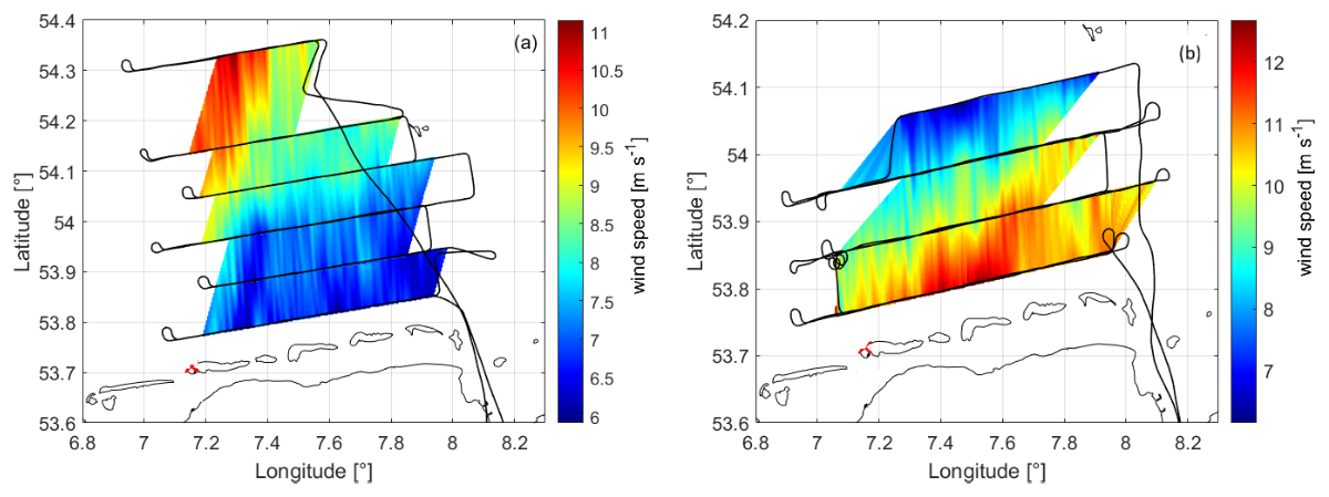
Figure 6 Contour plot of interpolated aircraft D-IBUF wind field measurements along the mean wind direction from the south at 100 m altitude, with the black line indicating the flight trajectory from 07:05 to 11:03 UTC on 23 July 2020 (a) and from 05:24 to 08:53 UTC on 23 September 2020 (b), as published in Cañadillas et al. (2023a).

3.5 Evaluation of numerical flow simulations

Airborne measurements offer significant potential for capturing atmospheric parameters during periods with meteorologically interesting flow conditions (e.g. stable stratification around and above offshore wind farms), which can be compared to simulations. Unlike many ground-based methods, they provide high-resolution data in the range of a few centimetres in both horizontal and vertical directions, often exceeding 1000 m in altitude. This makes them a valuable tool for comparison with simulations and for evaluating parameterizations in numerical models, including those related to wind turbines and turbulence, particularly in complex flow regimes such as those found in offshore environments (e.g. Siedersleben et al., 2018a; Platis et al., 2020; Cañadillas et al., 2023a).

3.5.1 Mesoscale simulations

Mesoscale simulations, such as those performed with WRF, experience intrinsic difficulties of direct comparison with single observations as provided by the different flights. WRF simulations suffer from time shifts (zum Berge et al., 2024) and an overall lack of detailed accuracy when single situations are considered. In particular, WRF simulations have generally shown difficulties in accurately representing atmospheric stability (Siedersleben et al., 2018a, b). These discrepancies are particularly pronounced near coastal regions, where deviations are larger compared to offshore locations over open water (Platis et al., 2020). Under stable conditions, the model struggles to accurately reproduce the altitude of the inversion layer (Siedersleben et al., 2020), as well as the coastal transition zone (Cañadillas et al., 2023a). The WRF model, using the wind farm parameterization by Fitch et al. (2012), was found to capture the horizontal extent of wakes well (Cañadillas et al., 2022). The agreement between lidar observations and WRF simulations including wind farm effects (WRF-WF) was generally good, with mean wind speed differences of approximately 2 %, although larger deviations occurred under stable atmospheric conditions. Both observations and simulations consistently show that the wind speed deficit extends above the upper tip height of the rotor (Siedersleben et al., 2018a). Several studies have used the airborne data set to first evaluate model performance and subsequently draw conclusions on wake behaviour and model representation (Larsen and Fischereit, 2021; van Stratum et al., 2022; Ali et al., 2023). Simulation progress has been achieved by coupling atmospheric and oceanic models. Nevertheless, current simulation approaches for representing wind-turbine-generated turbulence do not fully reproduce observations, particularly regarding the vertical transport of turbulent kinetic energy and its impact on the sea surface (Larsen et al., 2024).

First modelling experiments indicate that the angle between wind and wave direction plays a role for the undisturbed wind profile upstream of wind farms, as aligned wind-wave directions result in a lower roughness length. This reduced friction leads to higher wind speed. Further, the angle between wind and wave direction influences the wind speed recovery in the downstream wakes, as opposing wind and wave direction lead to more vertical mixing and therefore shorter wakes (Porchetta et al., 2021; Christiansen et al., 2022; Schmitt et al., 2026).

3.5.2 Engineering models

Engineering models, such as FLORIS (Gebraad et al., 2016), PyWake (Pedersen et al., 2023), Open Wind (UL-International, 2020), and FOXES (Schmidt et al., 2023), are widely used to optimize wind farm layouts and estimate energy production. Since this optimization process requires a large number of simulations across various configurations, the underlying wake models must be computationally efficient. Consequently, the flow within and around wind farms is typically strongly simplified by analytical, e.g. Gaussian, models that describe the wake decay downstream of individual turbines, which are then superposed (Cañadillas et al., 2023b). By design, since they are simplifications of mean momentum equations, engineering models cannot match the instantaneous turbulent flow. Also since they do not have a clear sensitivity to several atmospheric parameters, it is necessary to sample over several different atmospheric states to get close to the fully neutral conditions they are often calibrated upon. While it is possible to collect measurements with the aircraft over multiple days, there is a lot of scatter in the atmospheric conditions, and therefore in the measured wind speed, wind direction, and atmospheric stability. Hence, with such large standard deviations, comparison to engineering models is generally challenging.

Despite their focus on representing the annual energy production in the long term correctly, several studies have used two-dimensional airborne measurements to compare wake recovery behind offshore wind farms with engineering model results. For example, Cañadillas et al. (2020) analysed data from a series of flights conducted within the wakes at various distances downstream of two wind farm clusters in the North Sea under different atmospheric stability conditions. The study concluded that engineering models, which are often configured for neutral conditions, tend to underestimate wake effects under stable stratification.

In a more recent study, zum Berge et al. (2024) applied several WRF and engineering models with different configurations – WRF with a wind farm parameterization (WRF-WF), an engineering model coupled to WRF (EM-WRF), a standard engineering model with a baseline calibration (EM-BL), a calibration aiming at strongly dampening wake recovery (EM-LR), and the TurbOPark model (Pedersen et al., 2022) of Ørsted (EM-TP) – to simulate large-scale cluster wakes over extended distances in the German Bight and compared the results with airborne measurements. Figure 7, reproduced from zum Berge et al. (2024), shows the comparison of measured and modelled wake recovery for a large offshore wind farm cluster. Overall, the engineering models showed good agreement with the observations in the immediate vicinity of the wind farms and up to 20–30 km downstream. However, their accuracy in predicting the wake-induced wind speed deficit declined significantly with increasing distance from the wind farm clusters. Specifically, as observed on Leg 6 in Fig. 7, the distinct drop in measured wind speed is not caused by the wind farms but is rather due to the spatial variability and the closer distance to the coast and/or a temporal change in the weather situation (e.g. cloud or rain formation) during the multi-hour measurement flight, which the steady-state engineering models fail to capture. Several models provide the same output for specific locations, and the corresponding lines overlap in Fig. 7. As the models are initialized with a uniform, undisturbed free-stream wind speed for each flight leg, they have the same background velocity at the lateral edges of the flight path or far downstream, where the wake has dissipated. Since no wake effect is computed in these regions, the models provide the exact same undisturbed background wind speed.

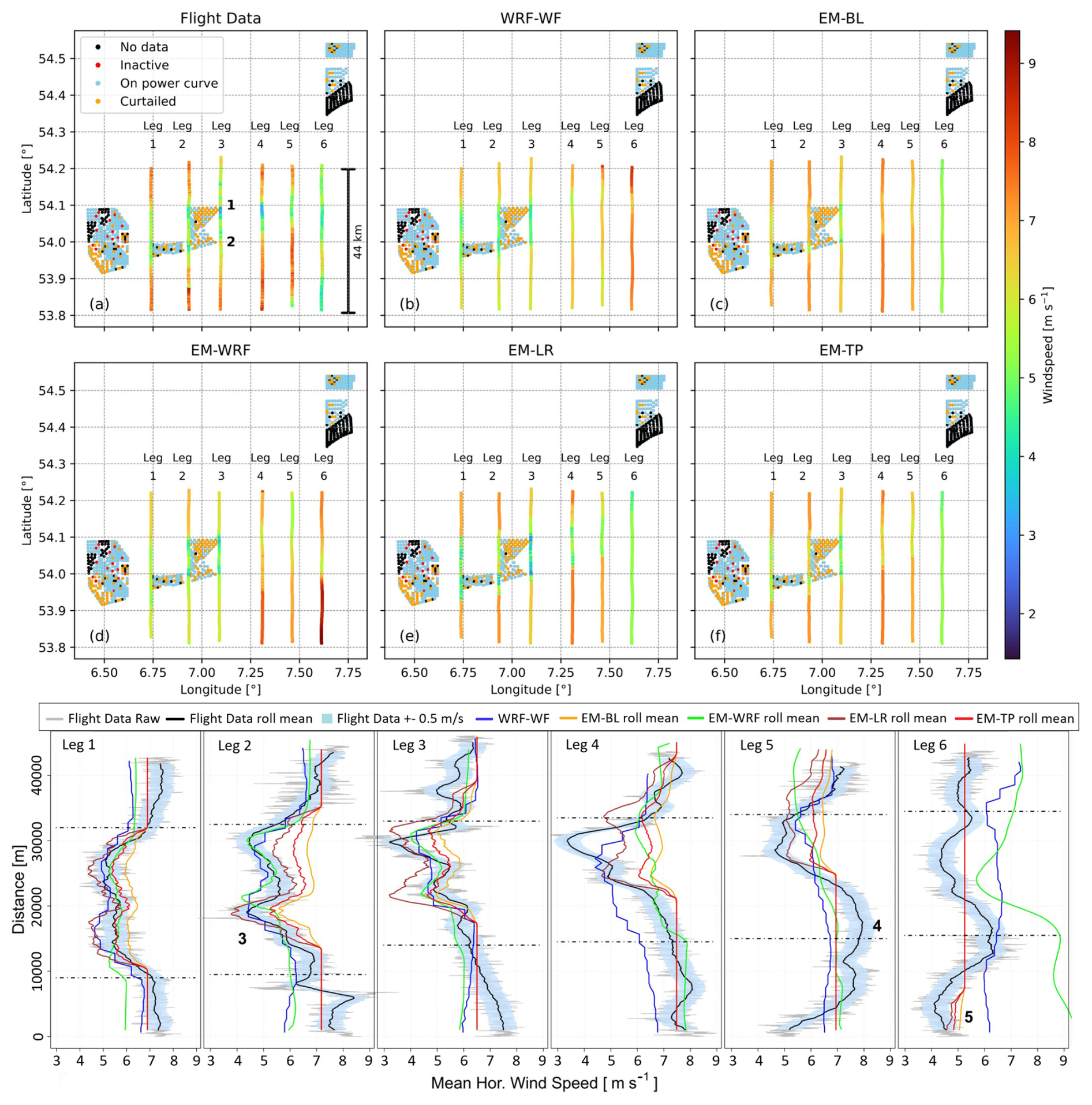
Figure 7 Top part: the measurement area in the German Bight with wind farm clusters N2, N3, and N4 on 14 July 2020 between 12:30–16:00 UTC. The dots represent the individual turbines and their operational status during the entire measurement time. (a) Results of the flight measurements on six flight legs with a mean wind direction of 270°. Results of the model calculations on the coordinates of the flight paths corresponding to (b) WRF-WF, (c) EM-BL, (d) EM-WRF, (e) EM-LR, and (f) EM-TP. Bottom part: the flight legs are shown as line plots with rolling-average filters for direct comparison. The dashed lines represent the estimated wake area. Graphic reproduced from zum Berge et al. (2024) (Fig. 7), licensed under CC BY-NC-ND 4.0 (https://creativecommons.org/licenses/by-nc-nd/4.0/, last access: 12 August 2026).

3.6 Sea state

As wind is a driving force for sea state development, the reduced wind speed downstream of wind farms leads to changes in the wave spectra. The enhanced laser scanner surface reflectance in wake areas (Platis et al., 2018) indicates that the water surface is smoother, and a larger percentage of the laser pulse is reflected back to the receiver. These changes in the surface roughness can take place on a horizontal scale of less than 1 km. Modifications of the wave spectra, i.e. the energy per wavelength, were observed in wake areas for developing sea state conditions (Bärfuss et al., 2020).

A significant reduction in wind speed in the wake of a wind farm also results in a decrease in significant wave height. Under stable atmospheric conditions, influences on sea state characteristics can be detected that can be attributed to a sea surface wake induced by the atmospheric wake. For the atmospheric wake, different parameters such as wind speed reduction are characteristic for the wake length. Characteristics for the sea surface wake can be selected as well. A simple, yet meaningful description can be provided by the reduction in the significant wave height (Schmitt et al., 2026). For all meander flights performed during WIPAFF and X-Wakes, the atmospheric wake length was found to be visible up to larger distances than wakes at the sea surface, defined as reduced significant wave height, but long-reaching surface wakes of several tens of kilometres have also been identified (Schmitt et al., 2026). More detailed analyses can be performed using the spectral sea surface energy distribution. Figure 8 shows such an energy distribution of the measurement flight on 24 July 2020. The area influenced by the wind farm is depicted within the manually inserted black lines, and from a graphical perspective, the wind originates from the left, i.e. from 270°. Within the black lines, a reduction in wind speed is observed, which can be noted as the wake of the wind farm. As the wind speed decreases, the energy density spectrum is also modified over a wide frequency range. This can be observed to a downstream distance of at least 29 km behind the wind farm. At downstream distances of 70 and 76 km, very low spectral energy densities are observed (black colour), particularly at angular frequencies below approximately 1.5 rad s⁻¹. Overall, the spectra at these large distances from the wind farm exhibit a more homogeneous distribution, with energy levels predominantly around 0.2 m² rad³ s⁻³ (green range of the colour scale), leaving low-energy regions to appear black due to the applied range. Wind farms can have a significant impact on developing sea state conditions, particularly on young wind waves. Reduced wind speed disrupts wave growth, resulting in a less energetic spectrum. A larger impact on sea conditions is observed for stable atmospheric conditions with more pronounced reductions in wind speed.

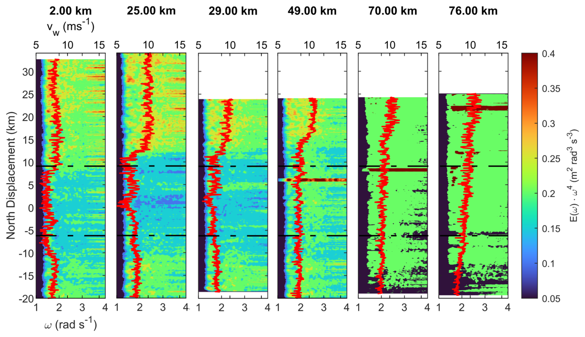
Figure 8 Sea surface energy distribution (colour-coded) for the flight on 24 July 2020 downstream of the wind farm clusters N2/N3 with stable atmospheric conditions. The airborne-measured wind speed is represented by the red lines. On that day, wind originated from 270° with a mean velocity of 10 m s⁻¹. The estimated wake region is depicted by the dashed lines. The horizontal, narrow lines with high energy density can be attributed to boats or other disturbances near the sea surface. The fact that similar disturbances appear across three different range panels (49, 70, and 76 km) at similar spatial positions suggests that the source was advected or moving during the measurement period. For each subplot, the downstream distance from the wind farm cluster is provided.

3.7 Global blockage effect

The global blockage effect (GBE) is the combined induction zone of all turbines in a wind farm (Porté-Agel et al., 2020). The upstream pressure field is responsible for deflecting the upstream flow to the side (Schneemann et al., 2025) and above the wind farm (Porté-Agel et al., 2020). The upward deflection reaches the upper atmospheric layers where stable stratification is always present and thus induces gravity waves that further intensify the GBE (Centurelli et al., 2021; Lanzilao and Meyers, 2024). Therefore, GBE depends on atmospheric boundary layer height and stratification of the inversion layer and the free atmosphere (Lanzilao and Meyers, 2024). Schneemann et al. (2021) also demonstrate that the GBE is sensitive to the stratification of the atmospheric boundary layer, as justified by Sanchez Gomez et al. (2023). It is still the subject of research if and to which extent it leads to a net power loss in a wind farm or rather a power redistribution (Lanzilao and Meyers, 2024). Compared to wind turbine or wind farm wake effects the GBE is much harder to investigate experimentally (Meijer et al., 2024). While wind speed gradients in wind farm wakes appear on the order of metres per second over short distances of some hundreds of metres (Schneemann et al., 2020), the wind speed gradient in GBE spreads over distances of several kilometres, with much smaller wind speed differences of only tenths of a metre per second (Schneemann et al., 2021). Similar to the previously described downstream wind farm wake investigations, airborne measurements with horizontal flight legs were performed upstream of wind farms. The flight path was oriented perpendicular to the main wind direction with the goal of quantifying GBE-induced wind speed differences in front of and beside the farm. The investigations were limited by the flight permission, which only allowed operation with a safety distance of at least 500 m to the wind turbines.

Figure 9 shows an exemplary data set and illustrates how the GBE was investigated: the flight patterns were aligned close to the wind farm cluster N4 with distances of 500 m to 2 km upstream. The wind speed was normalized to 1 in the undisturbed areas next to the areas affected by wakes, and latitudinal and longitudinal transects are displayed. Based on all flights with such patterns, small average numbers of wind speed reductions in the wake areas compared to the undisturbed areas were observed in the range of 2 % for the closest flight distance of 500 m with a high scatter. On averaged data, a non-significant trend of reduced wind speed in the direction towards the farm is visible, which cannot be reliably attributed to GBE. In this overview, different days with different atmospheric conditions are compared. The wind speed difference is calculated over large distances not considering mesoscale changes in the wind field. In summary, it turned out that the GBE is potentially too small to be determined by airborne measurements for single flights and also on average.

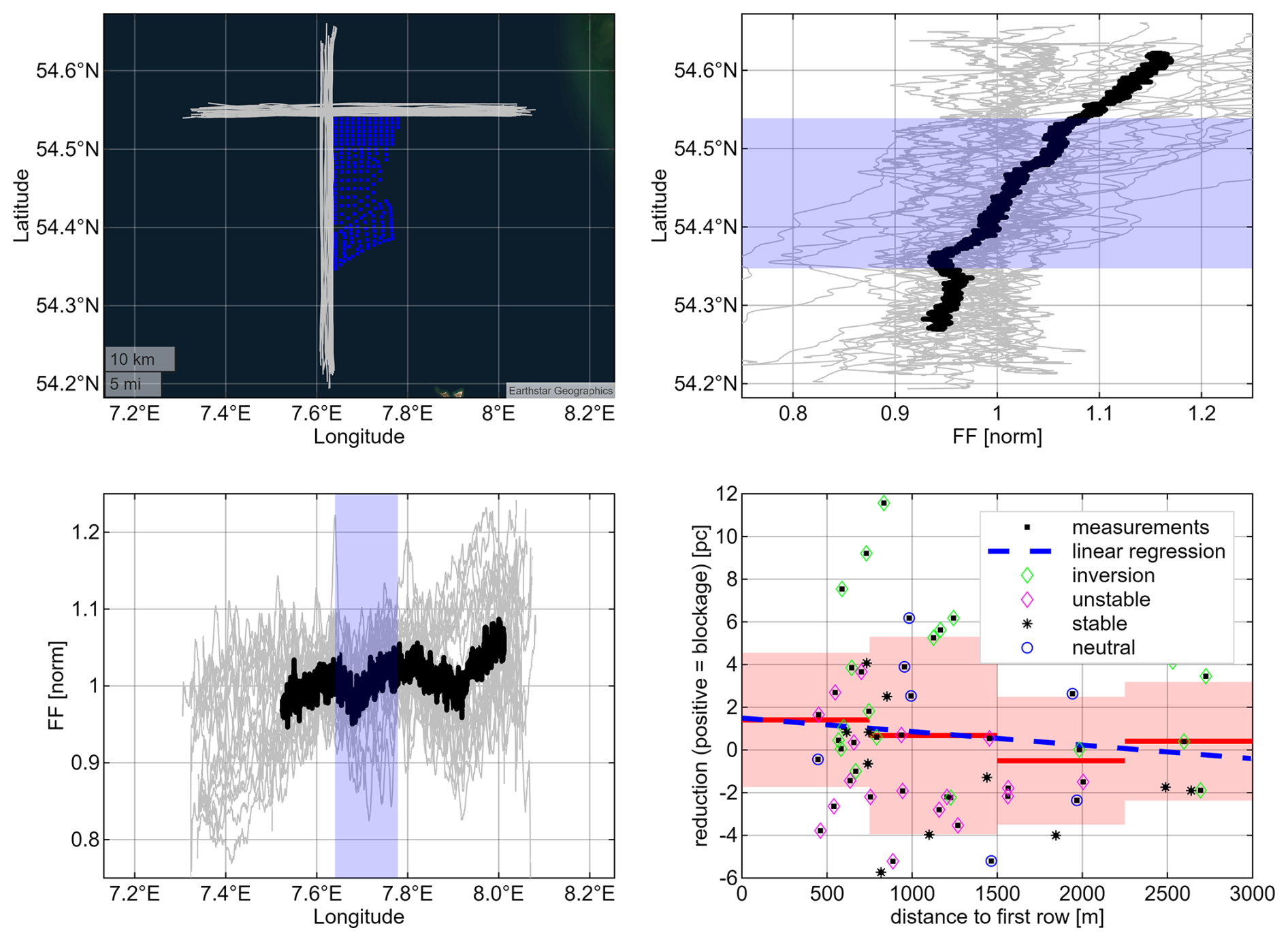
Figure 9 Airborne investigation of the blockage effect for wind from north and west. Upper left: flight sections (in white) used for investigation of the blockage effect around the wind farms (single wind turbines in blue). The sections were flown on different days and at different distances in front of the first wind turbine row. Upper right: this panel shows the unfolding of all meridional measurement sections on latitude vs. normalized wind speed (normalized by the median wind speed outside the wake for the leg regarded). The averaged normalized wind speed is shown with a thick black line. Lower left: this panel shows the unfolding of all longitudinal measurement sections on longitude vs. normalized wind speed (normalized by the median wind speed outside the wake for the leg regarded). The averaged normalized wind speed is shown with a thick black line. Lower right: statistical results – relative wind speed reduction which could be caused by the GBE over measurement leg distance. The single measurement legs used for the analysis are shown as black dots, with an overlaying marker for inversion/unstable/stable and neutral conditions. Average relative wind speed reduction is shown as a red line for each distance band, with an underlying reddish region indication standard deviation (1σ). The dashed blue line is the first-order polynomial regression on average relative wind speed reduction vs. distance to the first row of the wind turbines.

4 Conclusions

In conclusion, aircraft-based measurements provide many advantages for wind energy investigations: they can be flexibly adapted to the wind direction to study wake effects, and they provide highly resolved data of air temperature, humidity, and wind speed and direction. This allows for vertical profile measurements to obtain a detailed description of the local atmospheric boundary layer, including the derivation of atmospheric stability as well as high-resolution horizontal measurements to quantify atmospheric structures spanning over large areas. Simultaneous measurements of atmospheric modifications and changes in the surface properties can be recorded. Airborne measurements can resolve the complex and height-dependent phenomena of wind field modifications for coastal transitions, and such data can help to understand and properly simulate mesoscale processes in offshore wind assessments. The extensive data sets of the research projects WIPAFF and X-Wakes are to date unique for flexibly characterizing the North Sea atmospheric boundary layer. Combining the airborne data with satellite investigations, stationary long-term measurements by meteorological masts or lidar systems, and numerical simulations shows great potential. Therefore, the airborne data sets obtained during the projects WIPAFF (Bärfuss et al., 2019; Lampert et al., 2020) and X-Wakes (Rausch et al., 2023a; Lampert et al., 2024) provide a valuable base for investigating offshore wind conditions and their interaction with wind farms.