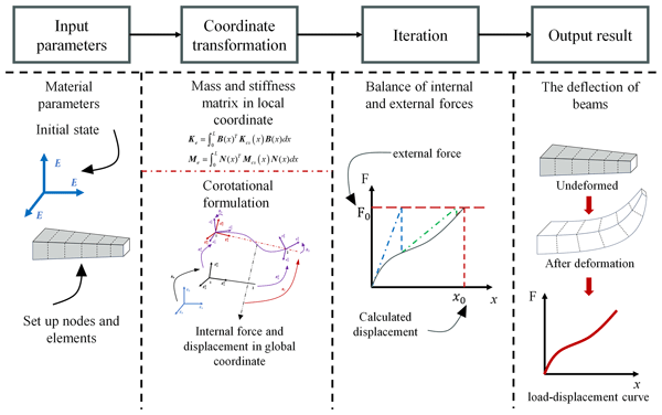
Geometric nonlinear analysis of Timoshenko beams with variable cross-section using co-rotational formulation

The geometrically nonlinear analysis of Timoshenko beams with variable cross-sections remains a challenging task in engineering practice, particularly for structures subjected to large deformations. While co-rotational (CR) formulations have been widely adopted for geometric nonlinear analysis, most existing CR-based beam models assume constant cross-sectional properties, limiting their applicability to beams with variable geometries. To overcome this limitation, this study introduces a novel co-rotational formulation specifically tailored for variable cross-section Timoshenko beams. The proposed approach integrates two key innovations: (1) the development of an improved spatial Timoshenko beam element employing analytical displacement shape functions to accurately capture bending deformation in variable cross-sections and (2) the introduction of an efficient Gaussian integration scheme for computing stiffness and mass matrices, eliminating the need for explicit moment-of-inertia evaluations at each cross-section. The tangent stiffness matrix is systematically derived within the co-rotational framework. The method is validated through five benchmark examples, including comparisons with experimental data and numerical results from the literature. Results demonstrate that the proposed model achieves superior computational accuracy and efficiency in handling large deformations, dynamic responses, and nonlinear behaviors of beams with irregular or proportionally graded cross-sections, offering a robust alternative to existing variable cross-section beam formulations.

1 Introduction

Beam structures are fundamental load-bearing components in various engineering disciplines, valued for their high strength, rigidity and low weight. Although uniform cross-section beams have been extensively studied, modern engineering applications increasingly utilize non-uniform flexible beams to optimize mass distribution and enhance mechanical performance in structures such as wind turbine blades, robotic manipulators, and aerospace components (Xiao et al., 2024; Elkaimbillah et al., 2021; Wang et al., 2014). These variable cross-section flexible beams frequently experience large deformations under operational loads, introducing geometric nonlinearities that invalidate classical linear beam theories based on small-deformation assumptions. Therefore, understanding the geometric nonlinearity of flexible beam structures with non-uniform cross-sections is essential for accurate engineering analysis of such structures.

Substantial research efforts have been dedicated to developing finite-element methodologies for the geometric nonlinear analysis of flexible beam structures. The most commonly used finite-element methods are the total Lagrangian (TL) (Heylinger and Asiri, 2020; Saravia et al., 2012; Marjamäki and Mäkinen, 2009) and updated Lagrangian (UL) (Greco et al., 2022; Turkalj et al., 2012; Kordkheili et al., 2011) formulations. While these approaches are widely adopted in commercial software due to their broad applicability, they have inherent limitations. Notably, these methods do not account for coordinate system changes following beam element deformation, leading to unacceptable calculation errors when elements undergo large rotations. To address this issue, an effective alternative for developing nonlinear beam elements is the co-rotational (CR) formulation. Research on CR finite elements begins with the pioneering work of Wempner (Wempner, 1969), Belytschko and Hsieh (Belytschko and Glaum, 1979), and Argyris and colleagues (Argyris et al., 1979). The key idea behind CR formulations is to decompose the motion of a beam element into the sum of a rigid body motion and a pure deformational displacement using a local reference coordinate system that continuously rotates and translates with the element. Pioneering work by Rankin et al. (Nour-Omid and Rankin, 1991; Rankin and Brogan, 1986) established a standard framework for calculating CR beam formulation. Another significant contribution to CR beam theory was made by Crisfield and his collaborators (Crisfield, 1990; Crisfield and Moita, 1996; Crisfield et al., 1997), who applied the CR formulation to solve various types of geometric nonlinearities and proposed a consistent method for computing element equilibrium equations. Behdinan et al. (Behdinan et al., 1998) extended the consistent CR static analysis to the dynamic analysis of beams undergoing large deflections. Hsiao et al. (Hsiao et al., 1999) introduced a consistent CR total Lagrangian finite-element formulation for the geometrically nonlinear dynamic analysis of Euler beams with large rotations but small strain. Early CR methods used different shape functions for computing elastic and inertial force vectors of the beam element, whereas Li et al. (Le et al., 2011, 2014) adopted cubic interpolations to formulate both inertia and internal local terms and employed their new CR formulation to perform nonlinear dynamic analysis of 2D and 3D beams. The computational efficacy and accuracy of CR approaches have further expanded their applications across various structural systems (Moon et al., 2023; Meng et al., 2016; Wang et al., 2018; Kim et al., 2022; Shen et al., 2021; Timoshenko et al., 1930). However, most existing CR formulations assume constant cross-sectional properties, significantly limiting their applicability to variable cross-section flexible beam designs.

The increasing use of non-uniform flexible beams has driven recent research into their nonlinear behavior. The analog equation method (Sapountzakis and Panagos, 2008a, b) has been employed for the nonlinear analysis of Timoshenko beams undergoing large deflections with variable cross-sections. Yu and Zhao (Yu et al., 2024) developed a viscoelastic beam element based on the absolute nodal coordinate formulation for various cross-sectional structures, where the modified Kelvin–Voigt viscoelastic constitutive model was introduced to describe the large deformation of viscoelastic materials. Building on this work, Yu et al. (Yu et al., 2024) further proposed an improved absolute nodal coordinate formulation for analyzing the nonlinear behavior of variable cross-sections with large aspect ratios. Elkaimbillah el al. (Elkaimbillah et al., 2021) employed Vlasov kinematics to develop a one-dimensional finite-element model for the nonlinear dynamic analysis of thin-walled composite beams with open variable cross-sections. Additional studies have focused on the nonlinear behavior of axially functionally graded beams with various cross-sections (Kumar et al., 2015; Ghayesh, 2018; Sınır et al., 2018; Xu et al., 2021). Regarding CR beam models for variable cross-sections, Nguyen and Gan (Nguyen, 2013; Nguyen and Gan, 2013) employed the CR beam element to investigate the large displacement of tapered cantilever beams made of axially functionally graded materials. Moon et al. (Moon, 2023Moon et al., 2023) extended the work of Crisfield (Crisfield and Moita, 1996) on CR beam elements by incorporating the fully populated and non-uniform cross-sectional stiffness matrix, expressed as a function of the axial length, to develop an anisotropic CR beam model for variable cross-sections. Nevertheless, current CR methods for non-uniform flexible beams remain constrained by computational inefficiency and limited precision.

Nevertheless, most existing CR formulations assume uniform cross-sectional properties, which significantly restricts their applicability to modern designs employing tapered or functionally graded beams. Although a few studies have attempted to incorporate cross-sectional variations within the CR framework, they often suffer from inadequate accuracy or computational inefficiency, especially when the cross-section changes abruptly, or the beam undergoes large rotations.

To overcome these persisting challenges, this paper presents a refined co-rotational beam model specifically designed for variable cross-sections, with three principal contributions.

A novel variable-cross-section Timoshenko beam element is formulated using analytical displacement shape functions derived from the equilibrium equations of a Timoshenko beam. This approach eliminates the truncation errors associated with standard polynomial interpolations and provides a more accurate description of the bending deformation, thereby enhancing the overall precision of the co-rotational procedure.

An efficient numerical integration strategy based on Gaussian quadrature is introduced to compute the element stiffness and mass matrices. This strategy avoids the need to explicitly evaluate the moment of inertia at each cross-section, leading to a substantial reduction in computational cost while maintaining accuracy.

A consistent tangent stiffness matrix is derived within the co-rotational framework, explicitly accounting for the geometric nonlinearities induced by large displacements and rotations. The formulation is general enough to accommodate both irregular and proportionally tapered cross-sections, extending the applicability of CR methods to a broader class of engineering structures.

The remainder of this paper is structured as follows: Sect. 2 develops the improved stiffness and mass matrices for the variable cross-section beam element. Section 3 describes the co-rotational formulation for geometric nonlinear analysis. Section 4 validates the proposed model through a series of benchmark examples, including constant and variable cross-section beams, a tapered frame, and a dynamic frequency analysis. Finally, the main conclusions of this investigation are thereafter summarized in Sect. 5.

2 The improved spatial Timoshenko beam element with variable cross-section

The CR method enables the use of linear Timoshenko beam elements to derive the tangent stiffness matrix in the global coordinate system. Typically, interpolated shape functions are employed to construct the beam element. However, most of these shape functions approximate beam displacements, which introduces truncation errors and decreases computational accuracy. In this section, an improved Timoshenko beam element with a variable cross-section is proposed to improve computational accuracy by employing analytical displacement shape functions for bending deformation. The specific process is outlined below.

As illustrated in Fig. 1, a beam with variable cross-section is considered. The beam element has a total length L, with the coordinate origin at the left end. The x axis is aligned with the longitudinal direction, while the y and z axes align with the principal axis of the cross-section. Typically, the displacement at any point within the spatial beam element is represented by $\mathit{\{}\mathit{u},\mathit{v},\mathit{w},{\mathit{\theta }}_x,{\mathit{\theta }}_y,{\mathit{\theta }}_z\mathit{\}}$, where u is the axial displacement along the x axis; v and w are the transverse displacements along the y and z axis, respectively; and θ_x, θ_y and θ_z denote the rotations about the x, y and z axis, respectively. The cross-section parameters are defined: where b is the width; h is the thickness; S is the cross-sectional area; and I_y and I_z are the moments of inertia about the y and z axis, respectively.

Figure 1 Variable geometric properties in a tapered beam.

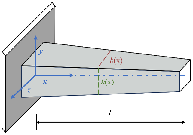
Define k_y and k_z as the cross-sectional non-uniformity coefficients along the y and z axes, respectively; E as the elastic modulus; G as the shear modulus; and J as the moment of inertia. Substituting the constitutive relations and geometric equations of the Timoshenko beam into the equilibrium equations yields

$$\begin{array}{}\text{(1)}& \left\{\begin{array}{l}\frac{\partial }{\partial x}\left[E{I}_y\frac{\partial {\mathit{\theta }}_y}{\partial x}\right]=k_{z}GA\left(\frac{\partial w}{\partial x}+{\mathit{\theta }}_y\right)\\ k_{z}GA\left(\frac{{\partial }^{\mathrm{2}}w}{\partial x^{\mathrm{2}}}+\frac{\partial {\mathit{\theta }}_y}{\partial x}\right)=\mathrm{0}\end{array}\right..\end{array}$$

For clarity and conciseness in presentation, the equilibrium equations are initially presented in the x–z plane (2D form). The formulation in the x–y plane is analogous, following the same principle by substituting corresponding variables (e.g., replacing w with v, θ_y with θ_z, I_y with I_z and k_z with k_y). This approach does not compromise generality, as the two bending directions are decoupled within the linear local element formulation.

The relationship between transverse displacement and bending displacement is given by

$$\begin{array}{}\text{(2)}& w=w_{\mathrm{b}}-{\displaystyle \frac{E{I}_y}{k_{z}GA}}{\displaystyle \frac{{\partial }^{\mathrm{2}}{w}_{\mathrm{b}}}{\partial x^{\mathrm{2}}}}+{\displaystyle \frac{E{I}_y}{k_{z}GA}}{\displaystyle \frac{{\partial }^{\mathrm{2}}{w}_{\mathrm{b}}}{\partial x^{\mathrm{2}}}}\left|x=\mathrm{0}\right.,\end{array}$$

where subscript b denotes contributions from bending deformation.

Similarly, the analytical solution of transverse displacement v satisfying the boundary conditions can be obtained as

$$\begin{array}{}\text{(3)}& v=v_{\mathrm{b}}-{\displaystyle \frac{E{I}_z}{k_{y}GA}}{\displaystyle \frac{{\partial }^{\mathrm{2}}{v}_{\mathrm{b}}}{\partial x^{\mathrm{2}}}}+{\displaystyle \frac{E{I}_z}{k_{y}GA}}{\displaystyle \frac{{\partial }^{\mathrm{2}}{v}_{\mathrm{b}}}{\partial x^{\mathrm{2}}}}\left|x=\mathrm{0}\right..\end{array}$$

Similar to the traditional Timoshenko beam element, the displacements in the u and θ_x are interpolated linearly, while the transverse displacements v_b and w_b are interpolated using cubic polynomial, and their expressions are given by

$$\begin{array}{}\text{(4)}& \left\{\begin{array}{l}u\left(x\right)=c_{\mathrm{1}}x+c_{\mathrm{2}}\\ {\mathit{\theta }}_x\left(x\right)=c_{\mathrm{11}}x+c_{\mathrm{12}}\\ v_{\mathrm{b}}\left(x\right)=c_{\mathrm{3}}{x}^{\mathrm{3}}+c_{\mathrm{4}}{x}^{\mathrm{2}}+c_{\mathrm{5}}x+c_{\mathrm{6}}\\ w_{\mathrm{b}}\left(x\right)=c_{\mathrm{7}}{x}^{\mathrm{3}}+c_{\mathrm{8}}{x}^{\mathrm{2}}+c_{\mathrm{9}}x+c_{\mathrm{10}}\end{array}\right..\end{array}$$

In general, the strain vector of a spatial Timoshenko beam element is expressed as

$$\begin{array}{}\text{(5)}& \left\{\begin{array}{l}\mathit{\epsilon }={\left[{\mathit{\epsilon }}_x,{\mathit{\gamma }}_y,{\mathit{\gamma }}_z,{\mathit{\gamma }}_x,{\mathit{\epsilon }}_y,{\mathit{\epsilon }}_z\right]}^{\mathrm{T}}\\ ={\left[\frac{\partial u}{\partial x},\frac{\partial v}{\partial x}-{\mathit{\theta }}_z,\frac{\partial w}{\partial x}+{\mathit{\theta }}_y,\frac{\partial {\mathit{\theta }}_x}{\partial x},\frac{\partial {\mathit{\theta }}_y}{\partial x},\frac{\partial {\mathit{\theta }}_z}{\partial x}\right]}^{\mathrm{T}}\\ ={\mathit{\epsilon }}_{\mathit{\alpha }}+{\mathit{\epsilon }}_{\mathit{\beta }}\end{array}\right.,\end{array}$$

where ${\mathit{\epsilon }}_{\mathit{\alpha }}={\left[\frac{\partial u}{\partial x},\frac{\partial v}{\partial x},\frac{\partial w}{\partial x},\frac{\partial {\mathit{\theta }}_x}{\partial x},\frac{\partial {\mathit{\theta }}_y}{\partial x},\frac{\partial {\mathit{\theta }}_z}{\partial x}\right]}^{\mathrm{T}}$, and ${\mathit{\epsilon }}_{\mathit{\beta }}={\left[\mathrm{0},-{\mathit{\theta }}_z,{\mathit{\theta }}_y,\mathrm{0},\mathrm{0},\mathrm{0}\right]}^{\mathrm{T}}$. By combining Eqs. (4) and (5), the expressions for the displacement and rotation vector u(x) of the beam can be obtained as follows:

$$\begin{array}{}\text{(6)}& \mathit{u}\left(x\right)=\mathbf{A}\left(x\right)\mathit{c},\end{array}$$

where the matrix A(x) represents the displacement–rotation coefficient matrix with respect to the shape function coefficient vector $\mathit{c}=\mathit{\{}{c}_{\mathrm{1}},\mathrm{\dots },c_{\mathrm{12}}{\mathit{\}}}^{\mathrm{T}}$. Taking the derivative of Eq. (6) yields

$$\begin{array}{}\text{(7)}& \left\{\begin{array}{l}\mathrm{d}\mathit{u}\left(x\right)={\left\{\frac{\partial u}{\partial x},\frac{\partial v}{\partial x},\frac{\partial w}{\partial x},\frac{\partial {\mathit{\theta }}_x}{\partial x},\frac{\partial {\mathit{\theta }}_y}{\partial x},\frac{\partial {\mathit{\theta }}_z}{\partial x}\right\}}^{\mathrm{T}}\\ \mathrm{d}\mathit{u}\left(x\right)=\mathrm{d}\mathbf{A}\left(x\right)\mathit{c}\end{array}\right..\end{array}$$

Based on the boundary conditions at x=0 and x=L, the relationship between the shape function coefficients and the nodal displacements can be derived and expressed in matrix form as follows:

$$\begin{array}{}\text{(8)}& \mathbf{H}\left(x\right)\mathit{c}=\mathit{d},\end{array}$$

where H(x) is the coefficient matrix of the shape function coefficients. The nodal displacement d is expressed as

$$\begin{array}{}\text{(9)}& \mathit{d}={\left\{u_{\mathrm{1}},v_{\mathrm{1}},w_{\mathrm{1}},{\mathit{\theta }}_{x\mathrm{1}},{\mathit{\theta }}_{y\mathrm{1}},{\mathit{\theta }}_{z\mathrm{1}},u_{\mathrm{2}},v_{\mathrm{2}},w_{\mathrm{2}},{\mathit{\theta }}_{x\mathrm{2}},{\mathit{\theta }}_{y\mathrm{2}},{\mathit{\theta }}_{z\mathrm{2}}\right\}}^{\mathrm{T}}.\end{array}$$

By substituting Eq. (9) into Eqs. (6) and (7), the following expressions are obtained:

$$\begin{array}{}\text{(10)}& {\displaystyle }\mathit{u}\left(x\right)=\mathbf{A}\left(x\right)\mathbf{H}(x{)}^{-\mathrm{1}}\mathit{d},\text{(11)}& {\displaystyle }\mathrm{d}\mathit{u}\left(x\right)=\mathrm{d}\mathbf{A}\left(x\right)\mathbf{H}(x{)}^{-\mathrm{1}}\mathit{d}.\end{array}$$

The relationship between the strain and nodal displacements of the element is then given by

$$\begin{array}{}\text{(12)}& \left\{\begin{array}{l}{\mathit{\epsilon }}_{\mathit{\alpha }}=\mathrm{d}\mathit{u}\left(x\right)=\mathrm{d}\mathbf{A}\left(x\right)\mathbf{H}(x{)}^{-\mathrm{1}}\mathit{d}\\ {\mathit{\epsilon }}_{\mathit{\beta }}={\mathbf{T}}_N\mathit{u}\left(x\right)={\mathbf{T}}_N\mathbf{A}\left(x\right)\mathbf{H}(x{)}^{-\mathrm{1}}\mathit{d}\\ \mathit{\epsilon }={\mathit{\epsilon }}_{\mathit{\alpha }}+{\mathit{\epsilon }}_{\mathit{\beta }}=\left[\mathrm{d}\mathbf{N}\left(x\right)+{\mathbf{T}}_N\mathbf{N}\left(x\right)\right]\mathit{d}=\mathbf{B}\left(x\right)\mathit{d}\end{array}\right.,\end{array}$$

where $\mathbf{N}\left(x\right)=\mathbf{A}\left(x\right)\mathbf{H}(x{)}^{-\mathrm{1}}$, $\mathrm{d}\mathbf{N}\left(x\right)=\mathrm{d}\mathbf{A}\left(x\right)\mathbf{H}(x{)}^{-\mathrm{1}}$, B(x) is the strain-displacement matrix, and T_N satisfies the following relationship:

$$\begin{array}{}\text{(13)}& {\mathbf{T}}_N=\left[\begin{array}{ll}\begin{array}{lll}\mathrm{0}& \mathrm{0}& \mathrm{0}\\ \mathrm{0}& \mathrm{0}& \mathrm{0}\\ \mathrm{0}& \mathrm{0}& \mathrm{0}\end{array}& \begin{array}{lll}\mathrm{0}& \mathrm{0}& \mathrm{0}\\ \mathrm{0}& \mathrm{0}& -\mathrm{1}\\ \mathrm{0}& \mathrm{1}& \mathrm{0}\end{array}\\ \begin{array}{lll}\mathrm{0}& \mathrm{0}& \mathrm{0}\\ \mathrm{0}& \mathrm{0}& \mathrm{0}\\ \mathrm{0}& \mathrm{0}& \mathrm{0}\end{array}& \begin{array}{lll}\mathrm{0}& \mathrm{0}& \mathrm{0}\\ \mathrm{0}& \mathrm{0}& \mathrm{0}\\ \mathrm{0}& \mathrm{0}& \mathrm{0}\end{array}\end{array}\right].\end{array}$$

By numerically integrating over the length L of the beam, the element stiffness matrix K_e and mass matrix M_e of the variable cross-section Timoshenko beam element are formulated as

$$\begin{array}{}\text{(14)}& \left\{\begin{array}{l}{\mathbf{K}}_{\mathrm{e}}=\underset{\mathrm{0}}{\overset{L}{\int }}\mathbf{B}\left(x{)}^{\mathrm{T}}{\mathbf{K}}_{\mathrm{cs}}\left(x\right)\mathbf{B}\right(x)\mathrm{d}x\\ {\mathbf{M}}_{\mathrm{e}}=\underset{\mathrm{0}}{\overset{L}{\int }}\mathbf{N}\left(x{)}^{\mathrm{T}}{\mathbf{M}}_{\mathrm{cs}}\left(x\right)\mathbf{N}\right(x)\mathrm{d}x\end{array}\right..\end{array}$$

Define J as the moment of inertia. The sectional stiffness matrix K_cs(x) for a variable cross-section beam is expressed as

$$\begin{array}{}\text{(15)}& {\mathbf{K}}_{\mathrm{cs}}\left(x\right)=\mathrm{diag}\left[\mathrm{ES}\left(x\right),k_y\mathrm{GS}\left(x\right),k_z\mathrm{GS}\left(x\right),\mathrm{GJ}\left(x\right),{\mathrm{EI}}_y\left(x\right),{\mathrm{EI}}_z\left(x\right)\right].\end{array}$$

Directly evaluating the integrals in Eq. (14) for variable cross-sections is often computationally intensive. Therefore, in this study, Gaussian quadrature is introduced to efficiently compute the element stiffness and mass matrices of the variable cross-section beam:

$$\begin{array}{}\text{(16)}& \left\{\begin{array}{l}{\mathbf{K}}_{\mathrm{e}}={\sum }_{i=\mathrm{1}}^n\frac{L}{\mathrm{2}}{\mathit{\omega }}_{\mathrm{i}}\mathbf{B}{\left(x_{\mathrm{i}}\right)}^{\mathrm{T}}{\mathbf{K}}_{\mathrm{cs}}\left(x_{\mathrm{i}}\right)\mathbf{B}\left(x_{\mathrm{i}}\right)\\ {\mathbf{M}}_{\mathrm{e}}={\sum }_{i=\mathrm{1}}^n\frac{L}{\mathrm{2}}{\mathit{\omega }}_{\mathrm{i}}\mathbf{N}{\left(x_{\mathrm{i}}\right)}^{\mathrm{T}}{\mathbf{M}}_{\mathrm{cs}}\left(x_{\mathrm{i}}\right)\mathbf{N}\left(x_{\mathrm{i}}\right)\end{array}\right.,\end{array}$$

where n is the number of Gaussian integration points, and ω_i and x_i are the corresponding weight coefficients and integration nodes, respectively.

The stiffness and mass matrices of the cross-section are determined based on the relevant parameters of the cross-section. Considering the diverse forms of cross-sections, a general formula is provided here to handle the cross-sectional parameters of variable cross-section beams with a certain taper.

Assume that the aspect ratio of the variable cross-section beam remains constant; i.e.,

$$\begin{array}{}\text{(17)}& {\displaystyle \frac{{\mathit{b}}_{\mathrm{r}}}{{\mathit{b}}_{\mathrm{l}}}}={\displaystyle \frac{{\mathit{h}}_{\mathrm{r}}}{{\mathit{h}}_{\mathrm{l}}}},\end{array}$$

where b_r and h_r are the width and thickness of the cross-section at the right end, and b_l and h_l are the width and thickness at the left end. Under this assumption, the cross-sectional parameters at any arbitrary point along the beam can be expressed as

$$\begin{array}{}\text{(18)}& \left\{\begin{array}{l}h\left(x\right)=k_{\mathrm{1}}x+f_{\mathrm{1}}\\ b\left(x\right)=k_{\mathrm{2}}h\left(x\right)=k_{\mathrm{2}}\left(k_{\mathrm{1}}x+f_{\mathrm{1}}\right)\\ S\left(x\right)=p_{\mathrm{1}}b\left(x\right)h\left(x\right)=p_{\mathrm{1}}{k}_{\mathrm{2}}{\left(k_{\mathrm{1}}x+f_{\mathrm{1}}\right)}^{\mathrm{2}}=k_{\mathrm{3}}{\left(k_{\mathrm{1}}x+f_{\mathrm{1}}\right)}^{\mathrm{2}}\\ I_{\mathrm{1}}\left(x\right)=p_{\mathrm{2}}b\left(x\right)h{\left(x\right)}^{\mathrm{3}}=p_{\mathrm{2}}{k}_{\mathrm{2}}{\left(k_{\mathrm{1}}x+f_{\mathrm{1}}\right)}^{\mathrm{4}}=k_{\mathrm{4}}{\left(k_{\mathrm{1}}x+f_{\mathrm{1}}\right)}^{\mathrm{4}}\end{array}\right..\end{array}$$

The calculation of the cross-sectional parameters for each cross-section requires solving for the corresponding coefficients f_l and $k_{\mathrm{i}}(i=\mathrm{1},\mathrm{3},\mathrm{4})$. The transition coefficients k₂, p₁ and p₂ do not need to be solved. This can be achieved by solving using the relevant parameters of the cross-section at both ends of the beam. For the fixed end of the beam, when x=0, we have h=h_l, S=S_max and I_y=I_ymax. When x=L, we have S=S_min and I_y=I_ymin. By substituting the known parameters of the beam at both ends into Eq. (18), we obtain

$$\begin{array}{l}{\displaystyle }{k}_{\mathrm{1}}=h_{\mathrm{1}}\left(\sqrt{{\displaystyle \frac{S_{\min }}{S_{\max }}}}\right)/L\\ {\displaystyle }{k}_{\mathrm{3}}=S_{\max }/h_{\mathrm{1}}^{\mathrm{2}}\\ \text{(19)}& {\displaystyle }{k}_{\mathrm{4}}=I_{y\max }/h_{\mathrm{1}}^{\mathrm{4}}.\end{array}$$

When the aspect ratio of the structure is variable, the width and thickness of the cross-section are mutually independent. By measuring the maximum thicknesses $h_{{\mathrm{l}}_{\max }}$ and $h_{{\mathrm{r}}_{\max }}$ of the cross-sections perpendicular to the y axis at both ends of the structure, the expression for the cross-sectional parameters at any point within the unit can also be derived. The variation pattern of cross-sections is classified into two categories:

1. Only partial cross-sectional moments of inertia and cross-sectional areas are known. In this paper, by assuming linear variation in width and thickness, the number of undetermined coefficients is reduced, which proves to be relatively accurate for the calculation of simple tapered beams. When calculating large deformations of beams with significantly tapered cross-sectional variations, higher-order interpolation is required for width and thickness. Each additional order introduces two additional undetermined coefficients, necessitating extra known conditions (such as cross-sectional areas and moments of inertia in the y and z directions at other sections). Only under these conditions can the derived shape function expressions accurately represent the large deformations of beams with notably tapered cross-sectional variations.

2. The specific expression for the variation in cross-sectional dimensions (such as width or diameter) is known. In this paper, the cross-sectional characteristics at the Gaussian integration points of the element can be directly computed using the expression for dimensional variation, and the solution is then obtained through Gaussian integration. Under such circumstances, this method demonstrates high accuracy and strong robustness even for nonlinearly varying cross-sectional dimensions.

Once the relevant coefficients are obtained, they can be substituted into the coordinates of the Gaussian integration points to calculate the cross-sectional parameters. By substituting the cross-sectional parameters into Eqs. (14) and (15), the element stiffness matrix K_e and the element mass matrix M_e of the variable cross-section Timoshenko beam element can be obtained.

3 Co-rotational formulation

The co-rotational formulation stands out by extracting the elastic deformation displacements from the overall displacements (Crisfield, 1990; Crisfield and Moita, 1996), thus predefining the projection relationship. The motion of the beam element from its initial state to the final deformed state is decomposed into rigid body motion and pure deformation. The rigid body motion component encompasses the rigid translation and rotation in the local reference coordinate system. Therefore, the core challenge of the co-rotational formulation lies in handling the coordinate transformation between different frames, thereby establishing the relationship between pure deformation and the overall deformation.

3.1 Definition and transformation of the reference coordinate system for spatial beam elements

For the spatial two-node beam element, the reference coordinate system is defined as shown in Fig. 2. The unit orthogonal vectors ${\mathit{E}}_{\mathrm{i}}i=\mathrm{1},\mathrm{2},\mathrm{3}$ represent the global reference system of the beam element, which remains fixed and unchanged. The unit orthogonal vectors ${\mathit{E}}_{\mathrm{i}}^{h}i=\mathrm{1},\mathrm{2},\mathrm{3}$ represent the local reference system of the beam element after rigid body motion, which continuously translates and rotates with the beam element. The local reference system ${\mathit{E}}_{\mathrm{i}}^{q}i=\mathrm{1},\mathrm{2},\mathrm{3}$ represents the original coordinate system of the beam element before deformation. Additionally, the vectors ${\mathit{e}}_{\mathrm{i}}^{\mathrm{1}}$ and ${\mathit{e}}_{\mathrm{i}}^{\mathrm{2}}$ define the cross-sectional reference system of the two nodes (1 and 2) of the beam.

Figure 2 Beam kinematics and coordinate systems.

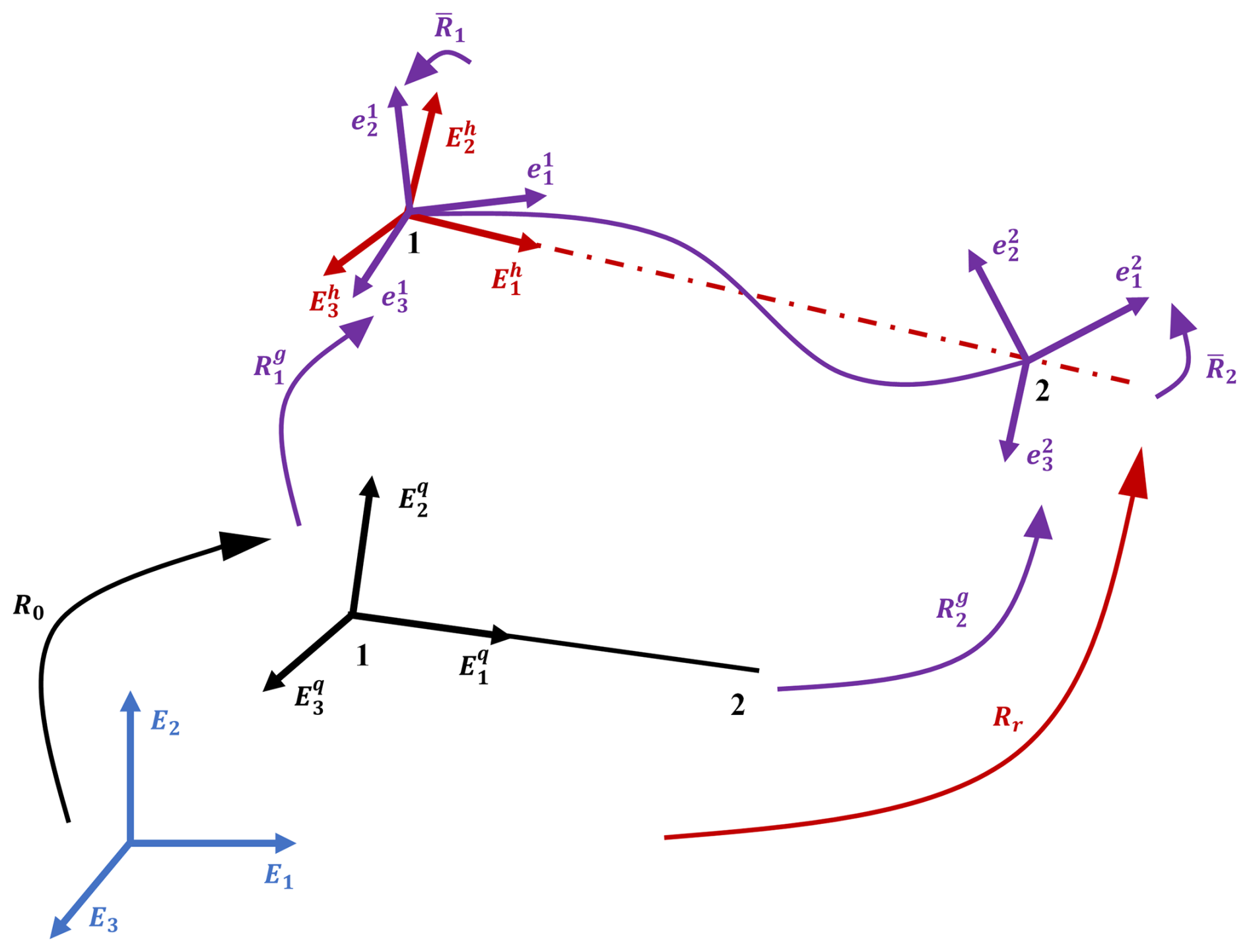
First, the rigid rotation of the local coordinate system ${\mathit{E}}_{\mathrm{i}}^h$ is addressed. The rigid rotation matrix R_r represents the transformation matrix from the reference system E_i to ${\mathit{E}}_{\mathrm{i}}^h$, and its expression is given by

$$\begin{array}{}\text{(20)}& {\mathbf{R}}_{\mathrm{r}}=\left[\begin{array}{lll}{r}_{\mathrm{1}}& r_{\mathrm{2}}& r_{\mathrm{3}}\end{array}\right].\end{array}$$

The vector r₁ is computed as the line connecting node 1 and node 2 of the beam element before and after deformation:

$$\begin{array}{}\text{(21)}& {\mathit{r}}_{\mathrm{1}}={\displaystyle \frac{{\mathbf{S}}_{\mathrm{2}}^{\mathrm{g}}-{\mathbf{S}}_{\mathrm{1}}^{\mathrm{g}}}{l}},\end{array}$$

where $s_i^{\mathrm{g}}$ represents the coordinates of node i in the global reference system after rigid rotation. The length l of the beam after deformation can be obtained by $l=∥s_{\mathrm{2}}^{\mathrm{g}}-s_{\mathrm{1}}^{\mathrm{g}}∥$.

The directions of the remaining two axes are determined by introducing an auxiliary vector q. The auxiliary vector serves two main purposes: (1) to solve the rigid rotation matrix in the global coordinate system and (2) to determine the differential relationship between the rigid rotation angle and the total displacement of the structure. Initially, the direction of q aligns with the local coordinate axis ${\mathit{E}}_{\mathrm{2}}^q$. After deformation of the beam element, the determination of the auxiliary vector q is related to the transformation of the local reference system:

$$\begin{array}{}\text{(22)}& {\displaystyle }{\mathit{q}}_{\mathrm{i}}={\mathbf{R}}_{\mathrm{i}}^{\mathrm{g}}{\mathbf{R}}_{\mathrm{0}}{\left[\begin{array}{lll}\mathrm{0}& \mathrm{1}& \mathrm{0}\end{array}\right]}^{\mathrm{T}}i=\mathrm{1},\mathrm{2},\text{(23)}& {\displaystyle }\mathit{q}={\displaystyle \frac{\mathrm{1}}{\mathrm{2}}}({\mathit{q}}_{\mathrm{1}}+{\mathit{q}}_{\mathrm{2}}),\end{array}$$

where ${\mathbf{R}}_{\mathrm{1}}^{\mathrm{g}}$ and ${\mathbf{R}}_{\mathrm{2}}^{\mathrm{g}}$ are the orthogonal matrices corresponding to the directions of the end nodes ${\mathit{e}}_{\mathrm{i}}^{\mathrm{1}}$ and ${\mathit{e}}_{\mathrm{i}}^{\mathrm{2}}$, respectively. q₁ and q₂ are the directions of the left and right end reference systems of the local reference system ${\mathit{E}}_{\mathrm{2}}^q$ after rigid rotation. R₀ denotes the initial orientation of the local coordinates, and q represents the direction of the local reference system ${\mathit{E}}_{\mathrm{2}}^q$ after rigid rotation.

By combining Eqs. (21), (22) and (23), the expressions for the remaining two components of the orthogonal matrix R_r can be obtained:

$$\begin{array}{}\text{(24)}& {\mathit{r}}_{\mathrm{3}}={\displaystyle \frac{{\mathit{r}}_{\mathrm{1}}\times \mathit{q}}{∥{\mathit{r}}_{\mathrm{1}}\times \mathit{q}∥}}{\mathit{r}}_{\mathrm{2}}={\mathit{r}}_{\mathrm{3}}\times {\mathit{r}}_{\mathrm{1}}.\end{array}$$

The local rotation matrix of the coordinate axis is defined as ${\stackrel{\mathrm{‾}}{\mathbf{R}}}_{\mathrm{i}}$, and the transformation from E_i to ${\mathit{e}}_{\mathrm{i}}^{\mathrm{1}}$ and ${\mathit{e}}_{\mathrm{i}}^{\mathrm{2}}$ can be expressed as follows:

$$\begin{array}{}\text{(25)}& {\mathbf{R}}_{\mathrm{r}}{\stackrel{\mathrm{‾}}{\mathbf{R}}}_{\mathrm{i}}={\mathbf{R}}_{\mathrm{i}}^{\mathrm{g}}{\mathbf{R}}_{\mathrm{0}}i=\mathrm{1},\mathrm{2}.\end{array}$$

Since ${\mathbf{R}}_{\mathrm{r}}^{\mathrm{T}}{\mathbf{R}}_{\mathrm{r}}=I$, Eq. (25) can be transformed as follows:

$$\begin{array}{}\text{(26)}& {\stackrel{\mathrm{‾}}{\mathbf{R}}}_{\mathrm{i}}={\mathbf{R}}_{\mathrm{r}}^{\mathrm{T}}{\mathbf{R}}_{\mathrm{i}}^{\mathrm{g}}{\mathbf{R}}_{\mathrm{0}}i=\mathrm{1},\mathrm{2}.\end{array}$$

Thus, the local rotation angles can be obtained as follows:

$$\begin{array}{}\text{(27)}& {\stackrel{\mathrm{‾}}{\mathit{\vartheta }}}_{\mathrm{i}}=\log \left({\stackrel{\mathrm{‾}}{\mathbf{R}}}_{\mathrm{i}}\right).\end{array}$$

3.2 Transformation of displacement vectors between the local and global coordinate systems

The global displacement vector of the beam element is defined as ${\mathit{P}}_{\mathrm{g}}^{\mathrm{g}}$, and the displacement vector in the local coordinate system after removing rigid body deformations is denoted as P_l. By utilizing the rotation framework described in the previous section, the local displacement P_l is obtained by subtracting the rigid body displacement from the total displacement ${\mathit{P}}_{\mathrm{g}}^{\mathrm{g}}$. The local internal force vector f_l and the tangent stiffness matrix K_l in the local coordinate system are computed through the transformation relationship between the two. The expression of the internal force vector F_g in the global coordinate system can be derived by balancing the internal virtual work in the global and local systems:

$$\begin{array}{}\text{(28)}& V=\mathit{\delta }{\mathit{P}}_{\mathrm{l}}^{\mathrm{T}}{f}_{\mathrm{l}}=\mathit{\delta }{\mathit{P}}_{\mathrm{g}}^{g\mathrm{T}}{\mathbf{F}}_{\mathrm{g}}.\end{array}$$

The variations in the displacement vectors ${\mathit{P}}_{\mathrm{g}}^{\mathrm{g}}$ and P_l can be expressed as follows:

$$\begin{array}{}\text{(29)}& {\displaystyle }\mathit{\delta }{\mathit{P}}_{\mathrm{l}}={\left[\begin{array}{lll}\mathit{\delta }\stackrel{\mathrm{‾}}{\mathit{u}}& \mathit{\delta }{\stackrel{\mathrm{‾}}{\mathit{\vartheta }}}_{\mathrm{1}}^{\mathrm{T}}& \mathit{\delta }{\stackrel{\mathrm{‾}}{\mathit{\vartheta }}}_{\mathrm{2}}^{\mathrm{T}}\end{array}\right]}^{\mathrm{T}},\text{(30)}& {\displaystyle }\mathit{\delta }{\mathit{P}}_{\mathrm{g}}^{\mathrm{g}}={\left[\begin{array}{llll}\mathit{\delta }{{\mathit{u}}_{\mathrm{1}}^{\mathrm{g}}}^{\mathrm{T}}& \mathit{\delta }{{\mathit{\theta }}_{\mathrm{1}}^{\mathrm{g}}}^{\mathrm{T}}& \mathit{\delta }{{\mathit{u}}_{\mathrm{2}}^{\mathrm{g}}}^{\mathrm{T}}& \mathit{\delta }{{\mathit{\theta }}_{\mathrm{2}}^{\mathrm{g}}}^{\mathrm{T}}\end{array}\right]}^{\mathrm{T}},\end{array}$$

where $\mathit{\delta }\stackrel{\mathrm{‾}}{\mathit{\vartheta }}\mathit{\_}\mathrm{i},(i=\mathrm{1},\mathrm{2})$ represents the variation in spatial rotation angles in the local coordinate system after considering rigid body deformations, and $\partial {\mathit{\theta }}_{\mathrm{i}}^{\mathrm{g}}(i=\mathrm{1},\mathrm{2})$ represents the variation in spatial rotation angles in the global coordinate system.

The variation in the transformation matrix involves the formation of a new matrix composed of rotational angles:

$$\begin{array}{}\text{(31)}& \mathit{\delta }{\stackrel{\mathrm{‾}}{\mathbf{R}}}_{\mathrm{i}}=\mathit{\delta }{\stackrel{\mathrm{̃}}{\stackrel{\mathrm{‾}}{\mathit{\theta }}}}_{\mathrm{i}}{\stackrel{\mathrm{‾}}{R}}_{\mathrm{i}},\end{array}$$

where the superscript tilde denotes the skew-symmetric matrix corresponding to a vector. A new local coordinate system, denoted as P_a, is defined based on Eqs. (29) and (31).

$$\begin{array}{}\text{(32)}& {\mathit{P}}_a={\left[\begin{array}{lll}\stackrel{\mathrm{‾}}{\mathit{u}}& {\stackrel{\mathrm{‾}}{\mathit{\theta }}}_{\mathrm{1}}^{\mathrm{T}}& {\stackrel{\mathrm{‾}}{\mathit{\theta }}}_{\mathrm{2}}^{\mathrm{T}}\end{array}\right]}^{\mathrm{T}}\end{array}$$

Let f_a represent the internal force vector corresponding to δP_a and K_l denote the transformed local stiffness matrix K_e obtained in Sect. 2 of this paper, which is converted to a 7-degree-of-freedom system. The transformation matrix between vectors P_a and P_l can be obtained through the transformation relationship of their respective stiffness matrices. The final conversion of K_l to K_a can be expressed as follows:

$$\begin{array}{}\text{(33)}& {\mathbf{K}}_a={\mathbf{B}}_{\mathrm{l}}^{\mathrm{T}}{\mathbf{K}}_{\mathrm{l}}{\mathbf{B}}_{\mathrm{l}}+{\mathbf{K}}_h{\mathbf{K}}_h=\left[\begin{array}{lll}\mathrm{0}& {\mathrm{0}}_{\mathrm{1}\times \mathrm{3}}& {\mathrm{0}}_{\mathrm{1}\times \mathrm{3}}\\ {\mathrm{0}}_{\mathrm{3}\times \mathrm{1}}& {\mathbf{K}}_{h\mathrm{1}}& {\mathrm{0}}_{\mathrm{3}\times \mathrm{3}}\\ {\mathrm{0}}_{\mathrm{3}\times \mathrm{1}}& {\mathrm{0}}_{\mathrm{3}\times \mathrm{3}}& {\mathbf{K}}_{h\mathrm{2}}\end{array}\right].\end{array}$$

The matrix B_l can be directly obtained by rotating the vector. The expressions for K_h1 and K_h2 are derived from the following equation:

$$\begin{array}{}\text{(34)}& {\displaystyle \frac{\partial }{\partial \stackrel{\mathrm{‾}}{\mathit{\theta }}}}\left[{\mathbf{T}}_s^{-T}\mathit{v}\right]={\displaystyle \frac{\partial }{\partial \stackrel{\mathrm{‾}}{\mathit{\vartheta }}}}\left[{\mathbf{T}}_s^{-T}\mathit{v}\right]{\displaystyle \frac{\partial \mathit{\vartheta }}{\partial \stackrel{\mathrm{‾}}{\mathit{\theta }}}}={\displaystyle \frac{\partial }{\partial \stackrel{\mathrm{‾}}{\mathit{\vartheta }}}}\left[{\mathbf{T}}_s^{-T}\mathit{v}\right]{\mathbf{T}}_s^{-\mathrm{1}},\text{(35)}& {\displaystyle }{\mathbf{T}}_s\left(\mathrm{\Phi }\right)={\displaystyle \frac{\sin \mathit{\phi }}{\mathit{\phi }}}\mathbf{I}+(\mathrm{1}-{\displaystyle \frac{\sin \mathit{\phi }}{\mathit{\phi }}})\mathit{e}{\mathit{e}}^{\mathrm{T}}+{\displaystyle \frac{\mathrm{1}}{\mathrm{2}}}({\displaystyle \frac{\sin (\mathit{\phi }/\mathrm{2})}{\mathit{\phi }/\mathrm{2}}}{)}^{\mathrm{2}}\stackrel{\mathrm{̃}}{\mathrm{\Phi }},\end{array}$$

where v represents the bending moment acting on the two ends of the internal force vector in the local coordinate system, e is the unit vector corresponding to the angle vector, and K_h1 and K_h2 correspond to ${\stackrel{\mathrm{‾}}{\mathit{\vartheta }}}_{\mathrm{1}}$ and ${\stackrel{\mathrm{‾}}{\mathit{\vartheta }}}_{\mathrm{2}}$ in Eq. (34). Consequently, the differential relationship between the rotational vector in the local coordinate system and the displacement vector in the global coordinate system can be derived as follows:

$$\begin{array}{}\text{(36)}& \begin{array}{rl}\left[\begin{array}{l}\mathit{\delta }{\stackrel{\mathrm{‾}}{\mathit{\theta }}}_{\mathrm{1}}\\ \mathit{\delta }{\stackrel{\mathrm{‾}}{\mathit{\theta }}}_{\mathrm{2}}\end{array}\right]& =\left(\left[\begin{array}{l}\begin{array}{llll}\mathrm{0}& \mathbf{I}& \mathrm{0}& \mathrm{0}\end{array}\\ \begin{array}{llll}\mathrm{0}& \mathrm{0}& \mathrm{0}& \mathbf{I}\end{array}\end{array}\right]-\left[\begin{array}{l}{\mathbf{G}}_{\mathit{\theta }}^{\mathrm{T}}\\ {\mathbf{G}}_{\mathit{\theta }}^{\mathrm{T}}\end{array}\right]\right){\mathit{E}}^{\mathrm{T}}\mathit{\delta }{\mathit{P}}_{\mathrm{g}}^{\mathrm{g}}\\ & =\mathit{P}{\mathit{E}}^{\mathrm{T}}\mathit{\delta }{\mathit{P}}_{\mathrm{g}}^{\mathrm{g}},\end{array}\end{array}$$

where ${\mathbf{G}}_{\mathit{\theta }}=\frac{\partial {\mathit{\theta }}_{\mathrm{r}}^e}{\partial {\mathit{P}}_{\mathrm{g}}^{\mathrm{g}}}$,$\mathit{E}=\mathrm{diag}\left[\begin{array}{llll}{\mathbf{R}}_{\mathrm{r}}& {\mathbf{R}}_{\mathrm{r}}& {\mathbf{R}}_{\mathrm{r}}& {\mathbf{R}}_{\mathrm{r}}\end{array}\right]$.

Thus, the relationship between δP_a and $\partial {\mathit{P}}_{\mathrm{g}}^{\mathrm{g}}$ can be obtained as follows:

$$\begin{array}{}\text{(37)}& \mathit{\delta }{\mathit{P}}_a={\mathbf{B}}_a\mathit{\delta }{\mathit{P}}_{\mathrm{g}}^{\mathrm{g}}{B}_a=\left[\begin{array}{l}\mathit{r}\\ \mathit{P}{\mathit{E}}^{\mathrm{T}}\end{array}\right],\end{array}$$

where $\mathit{r}=\left[\begin{array}{llll}-{\mathit{r}}_{\mathrm{1}}^{\mathrm{T}}& {\mathbf{0}}_{\mathrm{1}\times \mathrm{3}}& {\mathit{r}}_{\mathrm{1}}^{\mathrm{T}}& {\mathbf{0}}_{\mathrm{1}\times \mathrm{3}}\end{array}\right]$. The matrix G_θ in Eq. (36) is related to $\mathit{\delta }{\mathit{\theta }}_{\mathrm{r}}^e$.

$$\begin{array}{}\text{(38)}& \mathit{\delta }{\stackrel{\mathrm{̃}}{\mathit{\theta }}}_{\mathrm{r}}^e={\mathbf{R}}_{\mathrm{r}}^{\mathrm{T}}\mathit{\delta }{\mathbf{R}}_{\mathrm{r}}\mathit{\delta }{\mathit{\theta }}_{\mathrm{r}}^e=\left[\begin{array}{l}-{\mathit{r}}_{\mathrm{2}}^{\mathrm{T}}\mathit{\delta }{\mathit{r}}_{\mathrm{3}}\\ -{\mathit{r}}_{\mathrm{3}}^{\mathrm{T}}\mathit{\delta }{\mathit{r}}_{\mathrm{1}}\\ {\mathit{r}}_{\mathrm{2}}^{\mathrm{T}}\mathit{\delta }{\mathit{r}}_{\mathrm{1}}\end{array}\right]\end{array}$$

The expression for r₁, r₂, r₃ and δr₁ can be easily obtained. As for δr₃, it is related to δq according to Eq. (23):

$$\begin{array}{}\text{(39)}& \begin{array}{rl}\mathit{\delta }\mathit{q}& ={\displaystyle \frac{\mathrm{1}}{\mathrm{2}}}\left(\mathit{\delta }{\mathbf{R}}_{\mathit{\gamma }}+\mathit{\delta }{\mathbf{R}}_{\mathit{\gamma }}\right){\mathbf{R}}_{\mathrm{0}}{\left[\begin{array}{lll}\mathrm{0}& \mathrm{1}& \mathrm{0}\end{array}\right]}^{\mathrm{T}}\\ & ={\displaystyle \frac{\mathrm{1}}{\mathrm{2}}}\left(\mathit{\delta }{\stackrel{\mathrm{̃}}{\mathit{\theta }}}_{\mathrm{1}}^{\mathrm{g}}{\mathit{q}}_{\mathrm{1}}+\mathit{\delta }{\stackrel{\mathrm{̃}}{\mathit{\theta }}}_{\mathrm{2}}^{\mathrm{g}}{\mathit{q}}_{\mathrm{2}}\right).\end{array}\end{array}$$

The expression of the matrix G_θ can be obtained through Eq. (39) and ${\mathbf{G}}_{\mathit{\theta }}=\frac{\partial {\mathit{\theta }}_{\mathrm{r}}^e}{\partial {\mathit{P}}_{\mathrm{g}}^{\mathrm{g}}}$. The detailed derivation can be found in Crisfield (1990). Equation (37) yields the relationship between the force vector in the global coordinates and the internal force vector in the local coordinates.

$$\begin{array}{}\text{(40)}& {\mathbf{F}}^{\mathrm{g}}={\mathbf{B}}_a^{\mathrm{T}}{\mathit{f}}_a\end{array}$$

Similarly, by considering the variation of the force vector in the global coordinates in Eq. (37), it can be obtained as follows:

$$\begin{array}{}\text{(41)}& \left\{\begin{array}{l}\mathit{\delta }{\mathbf{F}}^{\mathrm{g}}={\mathbf{B}}_a^{\mathrm{T}}\mathit{\delta }{\mathit{f}}_a+\mathit{\delta }{\mathit{r}}^{\mathrm{T}}{\mathit{f}}_{a\mathrm{1}}+\mathit{\delta }\left(\mathit{E}{\mathit{P}}^{\mathrm{T}}\right)\mathbf{m}\\ \mathbf{m}={\left[\begin{array}{ll}\begin{array}{lll}{f}_{a\mathrm{2}}& f_{a\mathrm{3}}& f_{a\mathrm{4}}\end{array}& \begin{array}{lll}{f}_{a\mathrm{5}}& f_{a\mathrm{6}}& f_{a\mathrm{7}}\end{array}\end{array}\right]}^{\mathrm{T}}\end{array}\right.,\end{array}$$

where $f_{\mathrm{ai}}(i=\mathrm{1},\mathrm{\dots },\mathrm{7})$ represents the components of the force vector f_a. In conclusion, the tangent stiffness matrix in the global coordinate system can be obtained as follows:

$$\begin{array}{}\text{(42)}& \left\{\begin{array}{l}{\mathbf{K}}^{\mathrm{g}}={\mathbf{B}}_a^{\mathrm{T}}{\mathbf{K}}_a{\mathbf{B}}_a+{\mathbf{K}}_m\\ {\mathbf{K}}_m=\mathbf{D}{f}_{a\mathrm{1}}-\mathit{E}{\mathbf{QG}}_{\mathit{\theta }}^{\mathrm{T}}{\mathit{E}}^{\mathrm{T}}+\mathit{E}{\mathbf{G}}_{\mathit{\theta }}\mathbf{ar}\end{array}\right.,\end{array}$$

where

$$\begin{array}{}\text{(43)}& {\displaystyle }\mathbf{D}=\left[\begin{array}{llll}\mathit{d}& \mathbf{0}& -\mathbf{d}& \mathbf{0}\\ \mathbf{0}& \mathbf{0}& \mathbf{0}& \mathbf{0}\\ -\mathbf{d}& \mathbf{0}& \mathit{d}& \mathbf{0}\\ \mathbf{0}& \mathbf{0}& \mathbf{0}& \mathbf{0}\end{array}\right]\mathit{d}={\displaystyle \frac{\mathrm{1}}{l}}\left(\mathbf{I}-{\mathit{r}}_{\mathrm{1}}{\mathit{r}}_{\mathrm{1}}^{\mathrm{T}}\right),\text{(44)}& {\displaystyle }\mathbf{Q}=\left[\begin{array}{l}{\stackrel{\mathrm{̃}}{Q}}_{\mathbf{1}}\\ {\stackrel{\mathrm{̃}}{Q}}_{\mathbf{2}}\\ {\stackrel{\mathrm{̃}}{Q}}_{\mathbf{3}}\\ {\stackrel{\mathrm{̃}}{Q}}_{\mathbf{4}}\end{array}\right]\mathbf{a}=\left[\begin{array}{l}\mathrm{0}\\ \mathit{\eta }\left(f_{a\mathrm{2}}+f_{a\mathrm{5}}\right)/l-\left(f_{a\mathrm{3}}+f_{a\mathrm{6}}\right)/l\\ \left(f_{a\mathrm{4}}+f_{a\mathrm{7}}\right)/l\end{array}\right],\text{(45)}& {\displaystyle }{\mathit{P}}^{\mathrm{T}}\mathbf{m}={\left[\begin{array}{llll}{\mathbf{Q}}_{\mathbf{1}}^{\mathrm{T}}& {\mathbf{Q}}_{\mathbf{2}}^{\mathrm{T}}& {\mathbf{Q}}_{\mathbf{3}}^{\mathrm{T}}& {\mathbf{Q}}_{\mathbf{4}}^{\mathrm{T}}\end{array}\right]}^{\mathrm{T}}.\end{array}$$

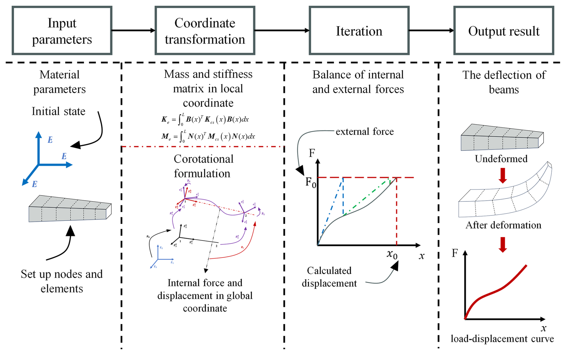
By utilizing the obtained tangent stiffness matrix, the difference in the global force vector can be calculated. The iterative process is employed to gradually converge the results towards the exact solution. The computational flowchart of nonlinear deformation in a variable cross-section beam is illustrated in Fig. 3.

Figure 3 Flowchart of nonlinear deformation in the variable cross-section beam.

4 Applications

This section presents comparative analysis between the proposed co-rotational Timoshenko beam model with a variable cross-section and existing benchmark results to validate its accuracy. The validation is carried out in three stages. First, the simple beam models with the constant cross-section are simulated to verify the proposed beam model with geometric nonlinearity. Second, the proposed co-rotational model is applied to a beam with variable cross-section and evaluated against both analytical solutions and numerical results from the literature, thereby confirming the capability of the proposed model in handling non-uniform geometries. Finally, a frequency analysis is conducted on a variable cross-section beam, and the computed results are compared with experimental measurements and published data to further demonstrate the capability of the developed beam element for dynamic analyses.

4.1 Application on constant cross-section beam element

4.1.1 Large-deformation analysis of spatially pre-bent cantilever beams subjected to concentrated loads

A 45° cantilever circular arc beam with a radius of R=100 m is subjected to a vertical concentrated load F of magnitude 300 N at its free end as shown in Fig. 4.

Figure 4 Pre-bent cantilever beam.

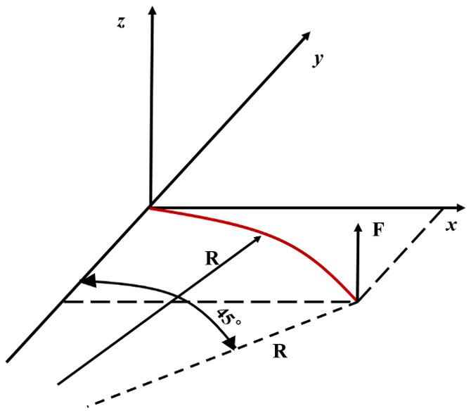
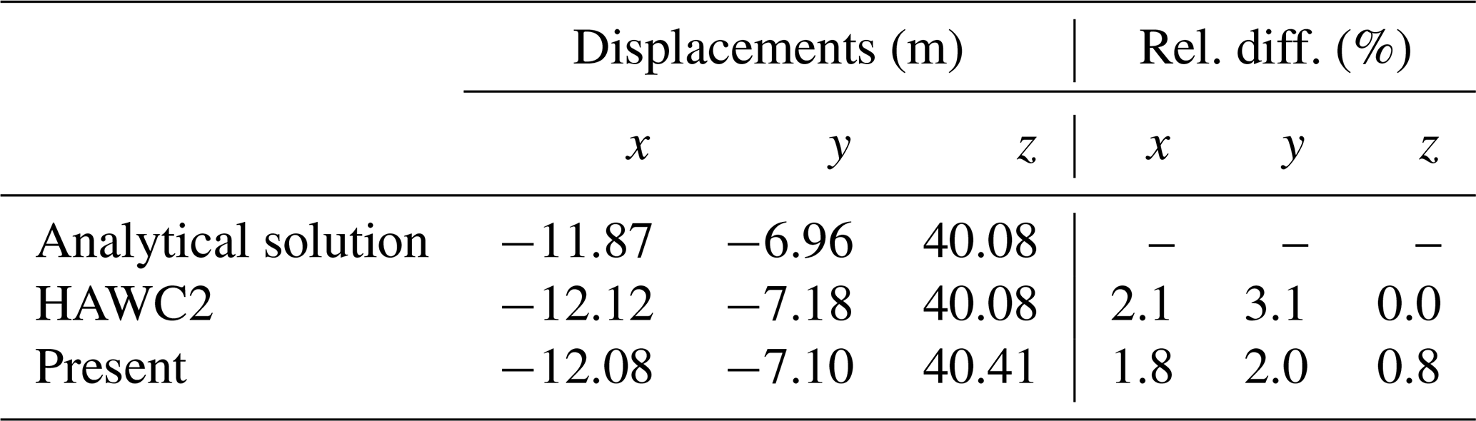
The beam is divided into eight elements, and the detailed cross-section properties of the beam are provided in Nguyen and Gan (2013). Table 1 presents a comparative analysis of the displacements at the free end of the beam in the x, y and z directions, as computed by the proposed method, the HAWC2 software and the analytical solution.

Table 1 shows that the obtained large deformations from the developed co-rotational beam model in the x and y directions are −12.08 and −7.10 m, respectively. Compared with the results obtained using HAWC2, the proposed approach improves the computational accuracy by 0.3 % in the x direction and 1.1 % in the y direction. The results confirm that the proposed model achieves high accuracy in capturing the large-deformation behavior of spatial Timoshenko beams.

Table 1 Comparison of the pre-bent beam tip displacements under a force applied at the free end.

4.1.2 Large-deformation analysis of a thin-plate beam under concentrated load

Figure 5 illustrates a cantilevered thin-plate beam with a total length of 0.51 m, a cross-sectional width of 30 mm and a thickness of 1 mm. The beam is made of 304 stainless steel, with a Young modulus of 193 GPa and a Poisson ratio of 0.3. To simulate concentrated loading, weights of 0.7 and 1.3 N are suspended from the free end of the cantilever beam. For each case, the actual horizontal displacement u and vertical displacement v at three selected points along the beam are measured. In this section, the proposed co-rotational beam model is employed to calculate the large deformation displacements of the cantilever beam under the two loading cases, and the plate beam is divided into nine elements. Table 2 compares the results from the present study, the experimental measurements and the data reported in Jiang et al. (2023).

Figure 5 Schematic diagram of thin-plate beam.

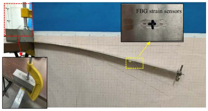
Table 2 Comparison of nodal displacements of the thin plates under free-end loading.

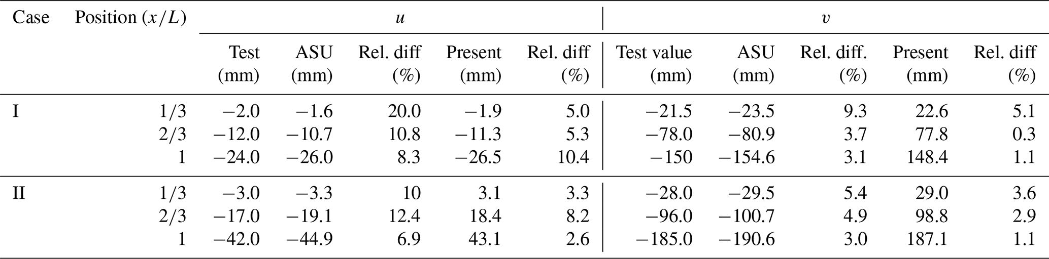
As shown in Table 2, except for case 1, where the relative error in the horizontal displacement at the free end reached 10.4 %, most of the other relative errors were within 10 %, and this error remains stable as the applied load increases. In terms of the vertical displacement v, the proposed model produces the results with relative errors below 5 %. Moreover, the predicted vertical deformation at the free end of the beam closely matches the measured values. These results validate the effectiveness and accuracy of the proposed model in capturing large elastic deformations in thin-walled flexible structures.

4.2 Numerical analysis of variable cross-section beams

To validate the performance of the proposed model in handling variable geometric configurations, numerical simulations are conducted on two variable cross-section beams. The results obtained using the proposed model are compared with those from relevant literature to assess its accuracy and effectiveness.

4.2.1 Numerical analysis of a rectangular variable cross-section cantilever beam

The cantilever beam with a rectangular cross-section, as shown in Fig. 6, is considered. The beam has a total length of 10 m and a constant width of b=0.25 m, and its thickness tapers linearly from 1.0 m at the fixed end to 0.2 m at the free end. The elastic modulus of the material is $E=\mathrm{3}\times {\mathrm{10}}^{\mathrm{4}}$ GPa, and the beam is subjected to a concentrated vertical load of 10 000 N at the free end. To evaluate the performance of the model, the beam is discretized into 10 elements. The computed deflection and rotation at the free end are compared with the exact analytical solution and results from alternative methods, as summarized in Table 3.

Figure 6 Simplified diagram of rectangular variable cross-section cantilever beam.

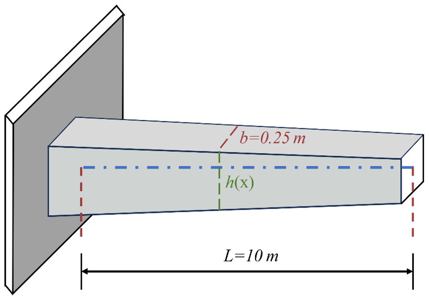
As shown in Table 3, the deflection and rotation results obtained using the proposed model align exceptionally well with the analytical solution. The predicted deflection at the free end is 0.01530 m, exactly matching the analytical value, and the computed rotation is 0.00399 rad, with a relative difference of only 0.25 %. In comparison, the segmental constant elements method yields a relative difference of 0.59 % in deflection and 2.00 % in rotation. This example demonstrates the effectiveness of the proposed co-rotational beam model in capturing the geometric nonlinear behavior of beams with varying cross-sections.

Table 3 Comparison of deflection and rotation at the free end of a rectangular variable cross-section cantilever beam.

4.2.2 Numerical simulation of a cantilever conical beam

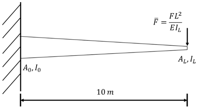
A variable cross-section cantilever beam, as shown in Fig. 7, is analyzed with a total length of 10 m. At the free end, both the moment of inertia I_L and cross-sectional area A_L are one-third of those at the fixed end. The ratio of the beam length to the height of the cantilever end section is 50:1. The material properties include an elastic modulus of 210 GPa and a shear modulus of 80.77 GPa. To facilitate comparison with existing numerical studies, a dimensionless load parameter $\stackrel{\mathrm{‾}}{\mathbf{F}}={\mathrm{FL}}^{\mathrm{2}}/{\mathrm{EI}}_L$, as defined in Marjamäki and Mäkinen (2009), is employed.

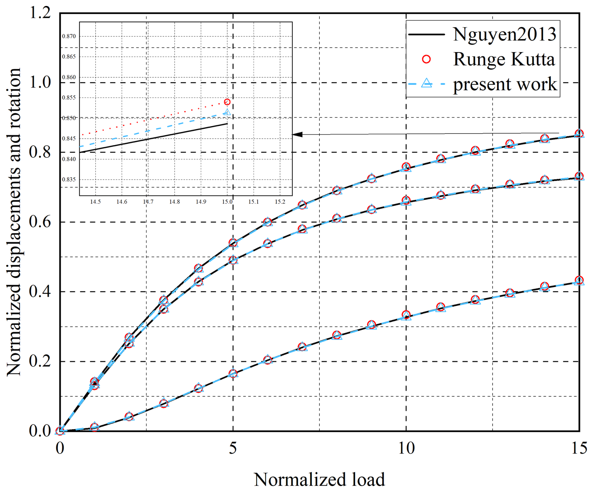
Figure 8 shows the load–displacement response of the conical cantilever beam subjected to a vertically downward point load at its free end. The results from the proposed co-rotational beam model are compared with the numerical solution obtained using the Runge–Kutta method from Marjamäki and Mäkinen (2009) and with finite-element results reported by Nguyen (Nguyen, 2013). As evident in Fig. 8, the response predicted by the proposed method aligns closely with the Runge–Kutta solution and shows improved agreement compared to Nguyen's finite-element results. This comparison validates the accuracy and effectiveness of the proposed co-rotational model in capturing large-deformation behavior in conical cantilever beams with variable cross-sections.

Figure 7 Conical beam.

Figure 8 Normalized moment and deformation in tapered beam.

4.3 Variable taper frame model

A well-known benchmark frame structure (Manuel et al., 1968), shown in Fig. 9, is commonly used to assess the performance of nonlinear analysis methods. In its original configuration, members AB and BC possess constant stiffness. Building upon this example, Francisco (de Araujo et al., 2017) proposed a modified version by introducing variable stiffness to column AB, as illustrated in Fig. 10. The cross-sectional properties at points A and B for this modified configuration are provided as follows:

$$\begin{array}{}\text{(46)}& \left\{\begin{array}{l}{I}_{xA}=\mathrm{14.76042}\times {\mathrm{10}}^{-\mathrm{8}}{\mathrm{m}}^{\mathrm{4}},I_{zA}=\mathrm{17.04167}\times {\mathrm{10}}^{-\mathrm{8}}{\mathrm{m}}^{\mathrm{4}}\\ I_{xB}=\mathrm{0.09375}\times {\mathrm{10}}^{-\mathrm{8}}{\mathrm{m}}^{\mathrm{4}},I_{zB}=\mathrm{0.27083}\times {\mathrm{10}}^{-\mathrm{8}}{\mathrm{m}}^{\mathrm{4}}\\ S_A=\mathrm{8.5}\times {\mathrm{10}}^{-\mathrm{4}}{\mathrm{m}}^{\mathrm{2}},S_B=\mathrm{1.0}\times {\mathrm{10}}^{-\mathrm{4}}{\mathrm{m}}^{\mathrm{2}}\end{array}\right..\end{array}$$

Beam BC retains a constant rectangular cross-section with S=0.006 m² and $I=\mathrm{2}\times {\mathrm{10}}^{-\mathrm{8}}$ m⁴. The material properties for the entire frame are assumed to be homogeneous, with an elastic modulus $E=\mathrm{7.2}\times {\mathrm{10}}^{\mathrm{9}}$ GPa and a Poisson ratio v=0.3. The frame is discretized into 20 elements, and the interpolation method proposed in this study is applied. The resulting vertical and horizontal displacements at the load application points are compared with those obtained from de Araujo et al. (2017) and a highly refined finite-element mesh reported in de Araujo et al. (2017). As shown in Fig. 11, the responses match quite well.

Figure 9 Frame scheme.

Figure 10 Column geometry.

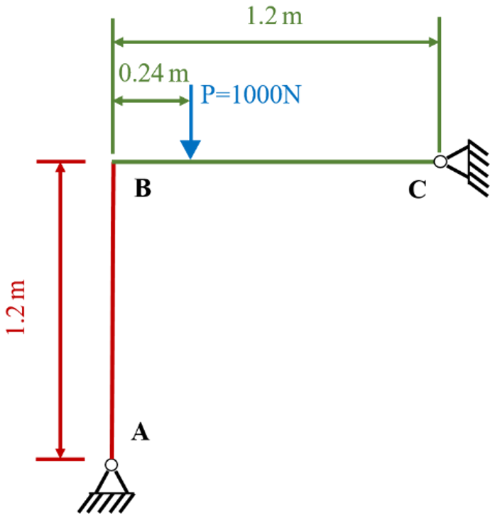
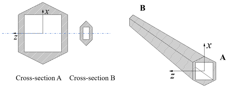
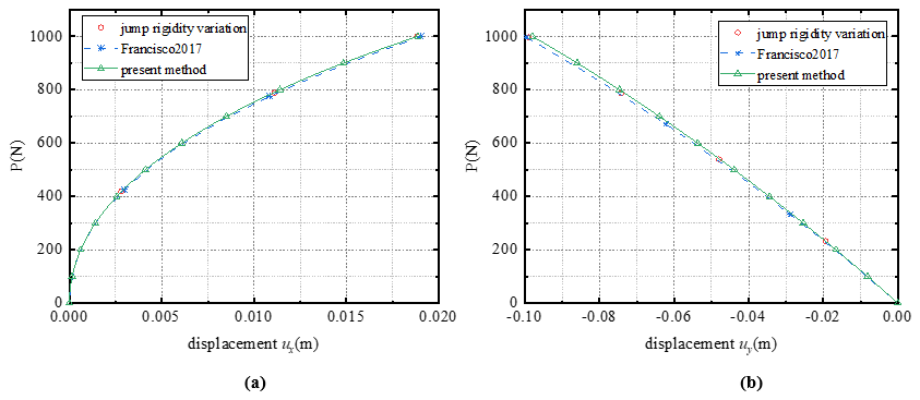
Figure 11 Frame displacement at node 13: (a) u_x displacement at node 13, (b) u_y displacement at node 13.

4.4 Natural frequencies of the conical cantilever beam

This section considers an experimental conical cantilever beam reported in Le et al. (2011) to verify the developed beam element. A modal analysis is performed where the natural frequencies are compared. The beam has a total length of 0.5 m, with a fixed-end section diameter of 0.03 m and a free-end section diameter of 0.005 m. The mass density and elastic modulus are 7800 kg m⁻³ and 210 GPa, respectively. The specific experimental setup is described in detail in Le et al. (2011). The first five natural frequencies of the conical beam are computed using the proposed variable cross-section beam model and are compared with both experimental results and two numerical approaches from Le et al. (2011). The comparison is presented in Table 4.

Table 4 Natural frequencies of the conical cantilever beam.

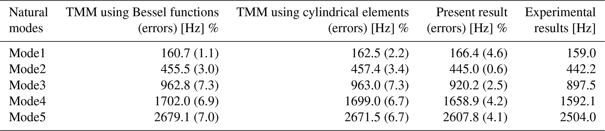
From Table 4, all three numerical methods produce results reasonably close to the experimental values. However, the proposed model demonstrates superior accuracy, with relative errors consistently below 5 % across all five modes. In contrast, the relative errors in the transfer matrix method (TMM) approaches in Le et al. (2011) exceed 5 % in several modes. Notably, the present model yields the most accurate results for the second and third modes, with relative errors of only 0.6 % and 2.5 %, respectively. These results confirm that the proposed variable cross-section beam model is effective in predicting the dynamic behavior of conical cantilever beams.

4.5 3D frame structure with variation in beam cross-sections

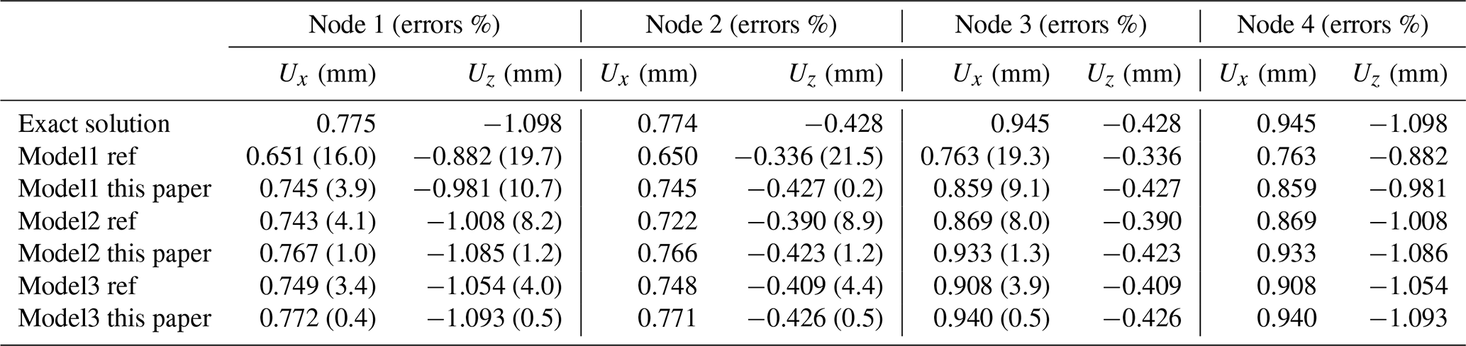
Figure 12 shows a 3D frame, with beams of varying circular cross-sections, loaded by concentrated load F at node 1. The displacements of nodes 1 to 4 were founded. Variation in the cross-sectional area of the beam a is defined by the following diameter quadratic function: $d\left(y\right)=\mathrm{0.04}+\mathrm{0.04}y\widehat{}\mathrm{2}$. The beams b and c have constant diameters through lengths of elements. Detailed parameters can be found in Murín and Kutiš (2002). Only one exact beam element was used to model each beam (a, b, c). In the Hermite beam element model, only one element was used to represent the beams b and c in all cases, but beam a was modeled with one, two and three elements in models 1, 2 and 3, respectively.

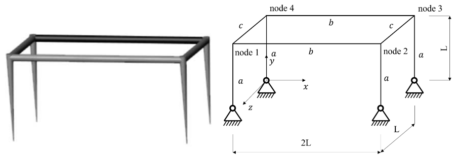
Figure 12 Frame displacement at node 13 (Murín and Kutiš, 2002).

The numerical results obtained by the present method are compared against those from the method proposed by Murín and Kutiš (2002) and the solutions from classical Hermite beam elements, as presented in Table 5. It can be observed from the table that compared to the reference method, the displacement solutions of the present method at all nodes and under all loading cases are consistently closer to the exact solution, demonstrating a significant enhancement in computational accuracy. Furthermore, when the number of elements is varied, the present method exhibits a narrower and more stable variation range in its solutions, highlighting its superior numerical robustness.

Table 5 Comparison of results.

5 Conclusions

This study proposes a novel co-rotational finite-element framework for the geometrically nonlinear analysis of variable cross-section Timoshenko beams, which significantly enhances computational accuracy, efficiency and robustness through the introduction of analytical displacement shape functions and a Gaussian integration strategy.

• Case 1. A variable cross-section beam element based on analytical displacement shape functions is proposed, replacing traditional interpolation functions and significantly enhancing computational accuracy in geometrically nonlinear analysis. Example 1 (large deformation of a uniform cross-section cantilever beam) and Example 3 (beam with constant taper) validate the accuracy of this element in capturing bending deformation, especially under variable cross-section conditions, where it demonstrates higher convergence accuracy compared to conventional piecewise uniform cross-section approaches.

• Case 2. Gaussian integration is introduced within the co-rotational framework to compute element matrices, eliminating the need for repeated moment-of-inertia calculations at each cross-section and thereby improving computational efficiency. Example 4 (large deformation of a linearly tapered beam) shows that the method maintains accuracy while outperforming existing variable cross-section co-rotational methods in computational efficiency; for cases with pronounced nonlinear taper, the method can be extended flexibly by incorporating additional sectional information.

• Case 3. A local-to-global coordinate transformation method tailored for variable cross-section beams is developed, capable of handling irregular and proportionally graded sections, thus extending the applicability of the co-rotational formulation. Example 2 (spatial beam large-deformation experiment) and Example 5 (frame structure with varying taper) demonstrate that the method retains good numerical stability and robustness in three-dimensional large-deformation analysis and complex geometric nonlinear problems. Example 6 further confirms the framework's suitability for spatially tapered beam analysis.

In summary, the proposed co-rotational model for variable cross-section beams exhibits clear advantages in accuracy, efficiency and generality, providing a reliable and efficient computational tool for predicting geometrically nonlinear responses of variable-section structures in engineering practice. Future work may focus on higher-order variable cross-section models, treatment of abruptly changing sections and multiphysics coupling problems.