Load application in wind turbine blades modelled as reduced-order multibody structures in the floating frame of reference formulation

Wind turbine aeroelastic simulation tools usually rely on the blade element momentum (BEM) theory to calculate aerodynamic loads and a beam finite element model for the structural response. A method to transfer distributed aerodynamic loads computed by these aeroelastic codes to a multibody reduced-order model based on the floating frame of reference formulation (FFRF) is presented. The model is based on solid finite elements, thus constituting a higher-fidelity alternative to beam elements, and the number of degrees of freedom (DOFs) is reduced using the Hurty/Craig-Bampton method, with interface reduction based on interface modes. The proposed method consists of calculating equivalent concentrated loads and applying them to the model using interpolation multipoint constraints (RBE3). Two approaches are introduced to avoid applying loads to the internal DOFs of the reduced-order model by including internal interfaces at the load application cross-sections, either described by interface modes or using a minimum strain energy formulation. Results show that adding load interfaces can improve the static response to torsional moments, but the overall increase in accuracy is not substantial; additionally, it is found that the reduced-order models built with minimum strain energy load interfaces demonstrate an increased stiffness. The methodology is also applied to a 12.6 m wind turbine blade, showcasing the better torsional response of the model when compared with standard beam models.

1 Introduction

The capacity and rotor size of wind turbines have greatly increased over the last decades. Longer and more flexible blades are now built, which experience large deflections under operation that can reach up to 20 % of their length (Gözcü and Dou, 2020). This brings new challenges to the aeroelastic modelling of wind turbines, which should not only capture the geometrical nonlinear effects inherent to large deflections but also other structural phenomena originating from the complex geometry and composite materials of wind turbine blades. Having a realistic and accurate structural model is essential to correctly predict wind turbines' power production, stability and loading conditions (Wang et al., 2016).

The wind turbine aeroelastic simulation tools currently available use beam-based models to represent the blades. Geometrically nonlinear effects are included by using either a nonlinear beam formulation, such as the geometrically exact beam theory (GEBT) (Reissner, 1973; Simo, 1985); or by modelling the blades as multibody systems using the floating frame of reference formulation (FFRF) (Shabana, 2020) with linear beam elements. The former strategy is implemented in OpenFAST (BeamDyn) (Wang et al., 2017), whereas the latter is employed in HAWC2 (Larsen and Hansen, 2021) or Bladed (DNV GL Energy, 2014), for example. This work focuses on the latter FFRF-based multibody approach, and HAWC2 is considered as the reference wind turbine aeroelastic code in this analysis.

In the FFRF, the motion of a body is described by the superposition of global rigid body motion and local deformation (assumed to be linear elastic), with respect to a body-fixed coordinate system, the floating frame (FF). This means that it is suited for bodies that undergo large rigid body displacements and rotations but only small local deformations and strains (Shabana, 2020; Zwölfer and Gerstmayr, 2020). To be able to compute large nonlinear deflections of wind turbine blades with this formulation, these need to be modelled as multiple sub-bodies, connected using constraint equations to ensure compatibility between them.

The structural model in HAWC2 follows this approach, having each sub-body composed of Timoshenko beam elements (Kim et al., 2013). Beam models have the advantage of being computationally efficient, but they are not as accurate as higher-fidelity finite element (FE) models, such as shell or solid element models. Recent verification studies (Antunes et al., 2024, 2025a) have concluded that specific effects disregarded by these beam models have a non-negligible influence on the nonlinear static response of slender and complex beam-like structures undergoing large deflections, as is the case of current wind turbine blades; cross-sectional deformation and three-dimensional effects are amongst such effects.

For this reason, although the model considered in this work is based on the multibody FFRF (similarly to HAWC2), it relies on solid elements to model the local deformation at the sub-body level (instead of beam elements), thus being able to account for the above-mentioned structural effects. However, for computational efficiency reasons, model order reduction techniques are additionally employed to reduce the number of flexible degrees of freedom (DOFs). Such a model is able to compute accurate nonlinear static responses when compared to standard solid finite element models, while having a lower number of DOFs (Antunes et al., 2025b). It is therefore relevant to assess its suitability for integration in a similar framework to that of wind turbine aeroelastic simulation tools using the same FFRF-based multibody approach (e.g. HAWC2).

One of the challenges in doing so relates to the application of external aerodynamic loads. In HAWC2 and most wind turbine aeroelastic simulation tools, the blade element momentum (BEM) theory (Glauert, 1935) is used to calculate the aerodynamic loads acting on the rotor blades (Madsen et al., 2020). Lift and drag forces per unit span of the blade are calculated at different spanwise locations, such that a distributed load is obtained along the blade span. For steady state operational conditions, these distributed loads predicted by BEM show good agreement with the higher-fidelity free-wake lifting-line (LL) method (Ramos-García et al., 2016, 2017) and 3D blade-resolved Reynolds-averaged Navier–Stokes (RANS) solvers, as shown for straight and curved blades in Li et al. (2022, 2025).

This type of load distribution is easily transferred to a beam model (one-dimensional) but not to a reduced-order structural model based on three-dimensional solid elements. Ideally, for such a model, it would be possible to apply the actual pressure distribution acting on the blade surface and therefore accompany the increase in structural model fidelity with an increase in fidelity of the aerodynamic model as well. However, this would result in a further increase in computational cost, which might not be justified given the stated accuracy of the BEM-based aerodynamic models currently available. Therefore, while it may constitute an important line of future research, this is outside the scope of this paper, which aims at evaluating the challenges in integrating a higher-fidelity structural model into HAWC2 (or similar wind turbine aeroelastic simulation tools) without further changes to the modelling of aerodynamic loads or other phenomena.

Consequently, alternative methods are required to apply this aerodynamic load distribution to the model considered here. The challenge lies not only in having a model based on solid elements but also in the fact that it is a reduced-order model, so not all physical DOFs are available to apply the loads. It is therefore important to assess whether the approximations introduced by this fact are acceptable or, if not, which methods can be adopted to have more realistic loads. This constitutes the main objective of this paper: to investigate different load application strategies for this model.

The paper is organised as follows: in Sect. 2, the FFRF-based reduced-order model from solid finite elements under analysis is described (Sect. 2.1), as well as the structural model in HAWC2 (Sect. 2.2); in Sect. 3, a summary of the loads acting on wind turbine blades and existing load transfer methods between aeroelastic models and high-fidelity FE models is presented, followed by a review of the challenges associated with applying such loads to the model under analysis and strategies used to surpass them (Sect. 3.1); in Sect. 4, the nonlinear static response of two structures is analysed under different load cases, to demonstrate the impact of the different load application challenges and strategies described: a simple isotropic beam and a 12.6 m wind turbine blade manufactured at DTU constitute the structures investigated, in Sect. 4.1 and 4.2, respectively.

2 Structural models

This study is focused on the FFRF-based reduced-order model built from solid finite elements presented in Antunes et al. (2025b). It uses the same baseline formulation as HAWC2, the floating frame of reference formulation (FFRF).

This formulation makes use of a body-fixed coordinate system – the floating frame (FF), defined with respect to a global inertial coordinate system – to describe the kinematics of the body. The global position of a point (${\mathit{r}}_j\in {\mathbb{R}}^{\mathrm{3}\times \mathrm{1}}$) in the body is expressed by its translational, rotational and flexible/elastic components (Shabana, 2020):

$$\begin{array}{}\text{(1)}& {\mathit{r}}_j={\mathit{q}}_{\mathrm{t}}+\mathbf{A}{\stackrel{\mathrm{‾}}{\mathit{u}}}_j,\end{array}$$

where ${\mathit{q}}_{\mathrm{t}}\in {\mathbb{R}}^{\mathrm{3}\times \mathrm{1}}$ is the position of the floating frame, ${\stackrel{\mathrm{‾}}{\mathit{u}}}_j\in {\mathbb{R}}^{\mathrm{3}\times \mathrm{1}}$ is the local position of the point (expressed in the FF) and $\mathbf{A}=\mathbf{A}\left(\mathit{\theta }\right)\in {\mathbb{R}}^{\mathrm{3}\times \mathrm{3}}$ is the orientation matrix of the FF (expressed in the global coordinate system), with $\mathit{\theta }\in {\mathbb{R}}^{n_{\mathrm{r}}\times \mathrm{1}}$ a rotational parameterisation with n_r rotational DOFs.

Recall that the main difference between the model being studied and HAWC2 lies in the formulation used to describe the local deformation of the body: while HAWC2 relies on Timoshenko beam elements, this model is based on solid finite elements in conjunction with model order reduction techniques. Additionally, a distinct version of the FFRF is adopted in the present model, denominated nodal-based FFRF. This means that the local position of a point in the body can be described directly by the nodal displacements, without the need to explicitly introduce the shape functions of the element in the formulation (Zwölfer and Gerstmayr, 2020).

Both HAWC2 and the present model account for nonlinear large deflections using the multibody approach: each structure is partitioned into multiple sub-bodies, each with its own FF, connected through constraint equations that ensure compatibility between connecting interfaces. In this regard, the difference lies in what constitutes an interface between sub-bodies in each model: in HAWC2, it corresponds to one beam node from each sub-body, whereas in the present model an interface is defined by multiple nodes reduced to a set of given DOFs with model order reduction techniques. Evidently, the constraint equations need to be adapted to the DOFs available in each case and are thus fundamentally different (Antunes et al., 2025b).

A more detailed description of these structural models is given in Sect. 2.1 and 2.2.

2.1 Multibody FFRF-based reduced-order model from solid finite elements

The model under analysis is described in detail in Antunes et al. (2025b). It is based on the nodal-based FFRF with projection-based model order reduction, as presented in Zwölfer and Gerstmayr (2021). The starting point is a flexible body discretised into displacement-based solid finite elements, with a total of n_n nodes.

Model order reduction (projection based) is introduced to approximate the nodal flexible displacements ${\stackrel{\mathrm{‾}}{\mathit{c}}}_{\mathrm{f}}\in {\mathbb{R}}^{\mathrm{3}{n}_{\mathrm{n}}\times \mathrm{1}}$, expressed in the FF $\left(\stackrel{\mathrm{‾}}{•}\right)$, by

$$\begin{array}{}\text{(2)}& {\stackrel{\mathrm{‾}}{\mathit{c}}}_{\mathrm{f}}=\stackrel{\mathrm{‾}}{\mathbf{\Psi }}\mathit{\zeta },\end{array}$$

where $\stackrel{\mathrm{‾}}{\mathbf{\Psi }}\in {\mathbb{R}}^{\mathrm{3}{n}_{\mathrm{n}}\times n_{\mathrm{f}}}$ is the reduction basis and $\mathit{\zeta }\in {\mathbb{R}}^{n_{\mathrm{f}}\times \mathrm{1}}$ denotes the n_f reduced flexible generalised coordinates. The FFRF coordinates thus read $\mathit{q}={\left[\begin{array}{ccc}{\mathit{q}}_{\mathrm{t}}^{\top }& {\mathit{\theta }}^{\top }& {\mathit{\zeta }}^{\top }\end{array}\right]}^{\top }$.

The global nodal positions $\mathit{r}\in {\mathbb{R}}^{\mathrm{3}{n}_{\mathrm{n}}\times \mathrm{1}}$ are calculated as

$$\begin{array}{}\text{(3)}& \mathit{r}={\mathbf{\Phi }}_{\mathrm{t}}{\mathit{q}}_{\mathrm{t}}+{\mathbf{A}}_{\mathrm{bd}}\stackrel{\mathrm{‾}}{\mathit{x}}+{\mathbf{A}}_{\mathrm{bd}}\stackrel{\mathrm{‾}}{\mathbf{\Psi }}\mathit{\zeta },\end{array}$$

where ${\mathbf{\Phi }}_{\mathrm{t}}={\left[\begin{array}{ccc}{\mathbf{I}}_{\left(\mathrm{3}\times \mathrm{3}\right)}& \mathrm{\cdots }& {\mathbf{I}}_{\left(\mathrm{3}\times \mathrm{3}\right)}\end{array}\right]}^{\top }\in {\mathbb{R}}^{\mathrm{3}{n}_{\mathrm{n}}\times \mathrm{3}}$ applies the FF translation q_t to all nodes, ${\mathbf{A}}_{\mathrm{bd}}=\mathrm{diag}(\mathbf{A},\mathrm{\cdots },\mathbf{A})\in {\mathbb{R}}^{\mathrm{3}{n}_{\mathrm{n}}\times \mathrm{3}{n}_{\mathrm{n}}}$ is a block-diagonal matrix containing the FF rotation matrix, and $\stackrel{\mathrm{‾}}{\mathit{x}}\in {\mathbb{R}}^{\mathrm{3}{n}_{\mathrm{n}}\times \mathrm{1}}$ is composed of the local reference (undeformed) nodal positions.

The equations of motion can be derived from Lagrange's equation, resulting in (Zwölfer and Gerstmayr, 2021)

$$\begin{array}{}\text{(4)}& \underset{\widehat{\mathbf{M}}}{\underbrace{{\mathbf{L}}^{\top }\stackrel{\mathrm{‾}}{\mathbf{M}}\mathbf{L}}}\ddot{\mathit{q}}+\underset{-{\widehat{\mathit{Q}}}_{\mathrm{v}}}{\underbrace{{\mathbf{L}}^{\top }\stackrel{\mathrm{‾}}{\mathbf{M}}\dot{\mathbf{L}}\dot{\mathit{q}}}}+\underset{-{\widehat{\mathit{Q}}}_{\mathrm{e}}}{\underbrace{{\mathbf{P}}^{\top }\stackrel{\mathrm{‾}}{\mathbf{K}}\mathbf{P}\mathit{q}}}+\underset{-{\widehat{\mathit{Q}}}_{\mathrm{c}}}{\underbrace{{\mathbf{J}}^{\top }\mathit{\lambda }}}=\underset{{\widehat{\mathit{Q}}}_{\mathrm{a}}}{\underbrace{{\mathbf{L}}^{\top }\mathit{f}}},\end{array}$$

where $\stackrel{\mathrm{‾}}{\mathbf{M}},\stackrel{\mathrm{‾}}{\mathbf{K}}\in {\mathbb{R}}^{\mathrm{3}{n}_{\mathrm{n}}\times \mathrm{3}{n}_{\mathrm{n}}}$ are, respectively, the constant FE mass and stiffness matrices from linear elastodynamics; λ are the Lagrange multipliers enforcing the constraint equations g=0; and $\mathit{f}\in {\mathbb{R}}^{\mathrm{3}{n}_{\mathrm{n}}\times \mathrm{1}}$ are the applied nodal forces. ${\widehat{\mathit{Q}}}_{\mathrm{a}}$ represents the applied forces, ${\widehat{\mathit{Q}}}_{\mathrm{c}}$ the constraint forces, ${\widehat{\mathit{Q}}}_{\mathrm{v}}$ the quadratic velocity vector and ${\widehat{\mathit{Q}}}_{\mathrm{e}}$ the elastic forces. Structural damping is not considered. However, Rayleigh proportional damping can be straightforwardly included.

The coordinate and constraint Jacobians are given by

$$\begin{array}{}\text{(5)}& {\displaystyle }\begin{array}{rl}\mathbf{L}& ={\displaystyle \frac{\partial \mathit{r}}{\partial \mathit{q}}}=\left[\begin{array}{ccc}\frac{\partial \mathit{r}}{\partial {\mathit{q}}_{\mathrm{t}}}& \frac{\partial \mathit{r}}{\partial \mathit{\theta }}& \frac{\partial \mathit{r}}{\partial \mathit{\zeta }}\end{array}\right]\\ & =\left[\begin{array}{ccc}{\mathbf{\Phi }}_{\mathrm{t}}& -{\mathbf{A}}_{\mathrm{bd}}{\stackrel{\mathrm{̃}}{\stackrel{\mathrm{‾}}{\mathit{r}}}}_{\mathrm{f}}\stackrel{\mathrm{‾}}{\mathbf{G}}& {\mathbf{A}}_{\mathrm{bd}}\stackrel{\mathrm{‾}}{\mathbf{\Psi }}\end{array}\right],\end{array}\text{(6)}& {\displaystyle }\mathbf{P}={\displaystyle \frac{\partial {\stackrel{\mathrm{‾}}{\mathit{c}}}_{\mathrm{f}}}{\partial \mathit{q}}}=\left[\begin{array}{ccc}{\mathbf{0}}_{\mathrm{3}{n}_{\mathrm{n}}\times \mathrm{3}}& {\mathbf{0}}_{\mathrm{3}{n}_{\mathrm{n}}\times n_{\mathrm{r}}}& \stackrel{\mathrm{‾}}{\mathbf{\Psi }}\end{array}\right],\text{(7)}& {\displaystyle }\mathbf{J}={\displaystyle \frac{\partial \mathit{g}}{\partial \mathit{q}}},\end{array}$$

where $\stackrel{\mathrm{‾}}{\mathbf{G}}$ relates the angular velocity $\stackrel{\mathrm{‾}}{\mathit{\omega }}\in {\mathbb{R}}^{\mathrm{3}\times \mathrm{1}}$ with the rotational parameterisation, as $\stackrel{\mathrm{‾}}{\mathit{\omega }}=\stackrel{\mathrm{‾}}{\mathbf{G}}\dot{\mathit{\theta }}$, and ${\stackrel{\mathrm{̃}}{\stackrel{\mathrm{‾}}{\mathit{r}}}}_{\mathrm{f}}\in {\mathbb{R}}^{\mathrm{3}{n}_{\mathrm{n}}\times \mathrm{3}}$ contains the vertically concatenated skew-symmetric matrices of the local nodal positions ${\stackrel{\mathrm{‾}}{\mathit{r}}}_{{\mathrm{f}}_j}={\stackrel{\mathrm{‾}}{\mathit{x}}}_j+{\stackrel{\mathrm{‾}}{\mathit{c}}}_{{\mathrm{f}}_j}\in {\mathbb{R}}^{\mathrm{3}\times \mathrm{1}}$.

To obtain the reduction basis $\stackrel{\mathrm{‾}}{\mathbf{\Psi }}$ in Eq. (2), the Hurty/Craig-Bampton method (Hurty, 1965; Craig and Bampton, 1968) and an interface reduction technique based on local interface modes (Krattiger et al., 2019) are applied sequentially to the FE system of equations. To do so, the flexible DOFs (nodal flexible displacements ${\stackrel{\mathrm{‾}}{\mathit{c}}}_{\mathrm{f}}$) are first partitioned into internal (i) and interface/boundary (b) DOFs. As illustrated in Fig. 1, the interface DOFs of each sub-body are composed of a minimum of two interfaces, here denoted by substructuring interfaces (B0 and B1), located at its ends. These allow the connection between sub-bodies.

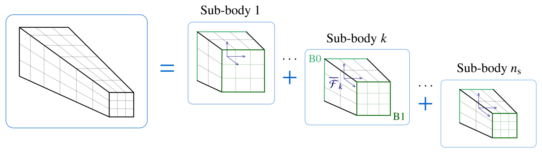
Figure 1 Structure partitioned into sub-bodies, each with its own floating frame ${\stackrel{\mathrm{‾}}{\mathcal{F}}}_k$ and two substructuring interfaces (B0, B1).

The Hurty/Craig-Bampton method eliminates the internal DOFs by approximating them with static modes augmented with a set of dynamic eigenmodes. Each static mode represents the static response of the internal DOFs to a unit displacement of 1 interface DOF, while keeping the remaining interface DOFs fixed. The dynamic eigenmodes, also named fixed-interface modes, are a truncated set of n_m eigenvectors calculated from the generalised eigenvalue problem considering the interface DOFs fixed:

$$\begin{array}{}\text{(8)}& \left({\stackrel{\mathrm{‾}}{\mathbf{K}}}_{ii}-{\mathit{\omega }}_m^{\mathrm{2}}{\stackrel{\mathrm{‾}}{\mathbf{M}}}_{ii}\right){\stackrel{\mathrm{‾}}{\mathit{\phi }}}_{i_m}=\mathbf{0},\end{array}$$

where ${\stackrel{\mathrm{‾}}{\mathit{\phi }}}_{i_m}\in {\mathbb{R}}^{n_i\times \mathrm{1}}$ represents the mth mode shape of the fixed-interface modes.

The Hurty/Craig-Bampton reduction basis ${\stackrel{\mathrm{‾}}{\mathbf{\Psi }}}_{\mathrm{HCB}}\in {\mathbb{R}}^{(n_i+n_b)\times (n_b+n_{\mathrm{m}})}$ is given by (Allen et al., 2020)

$$\begin{array}{}\text{(9)}& \begin{array}{rl}& {\stackrel{\mathrm{‾}}{\mathbf{\Psi }}}_{\mathrm{HCB}}=\left[\begin{array}{cc}{\stackrel{\mathrm{‾}}{\mathbf{\Psi }}}_{\mathrm{HCB}}^{(\mathrm{stat}.)}& {\stackrel{\mathrm{‾}}{\mathbf{\Psi }}}_{\mathrm{HCB}}^{(\mathrm{dyn}.)}\end{array}\right]=\left[\begin{array}{cc}\mathbf{I}& \mathbf{0}\\ -{\stackrel{\mathrm{‾}}{\mathbf{K}}}_{ii}^{-\mathrm{1}}{\stackrel{\mathrm{‾}}{\mathbf{K}}}_{ib}& {\stackrel{\mathrm{‾}}{\mathbf{{\rm Y}}}}_i\end{array}\right]\\ & \text{with}{\stackrel{\mathrm{‾}}{\mathbf{{\rm Y}}}}_i=\left[\begin{array}{ccc}{\stackrel{\mathrm{‾}}{\mathit{\phi }}}_{i_{\mathrm{1}}}& \mathrm{\cdots }& {\stackrel{\mathrm{‾}}{\mathit{\phi }}}_{i_{n_{\mathrm{m}}}}\end{array}\right].\end{array}\end{array}$$

The reduced generalised flexible coordinates ζ are thus composed of the interface flexible nodal displacements ${\stackrel{\mathrm{‾}}{\mathit{c}}}_{{\mathrm{f}}_b}\in {\mathbb{R}}^{n_b\times \mathrm{1}}$ and the modal participation factors ${\mathit{\xi }}_i\in {\mathbb{R}}^{n_{\mathrm{m}}\times \mathrm{1}}$ of the fixed-interface modes.

The resulting Hurty/Craig-Bampton reduced FE system matrices (${\stackrel{\mathrm{‾}}{\mathbf{M}}}_{\mathrm{HCB}},{\stackrel{\mathrm{‾}}{\mathbf{K}}}_{\mathrm{HCB}}$) can still be large, depending on the number of interface nodes and the discretisation of the solid FE model. For this reason, an interface reduction method is also employed, which applies an additional approximation to the interface DOFs only:

$$\begin{array}{}\text{(10)}& {\stackrel{\mathrm{‾}}{\mathit{c}}}_{{\mathrm{f}}_b}={\stackrel{\mathrm{‾}}{\mathbf{\Psi }}}_b{\mathit{\zeta }}_b.\end{array}$$

In this case, the interface DOFs are approximated as a linear combination of mode shapes, calculated from the generalised eigenvalue problem, defined considering the portion of the Hurty/Craig-Bampton reduced-system matrices relative to the interface DOFs:

$$\begin{array}{}\text{(11)}& \left({\stackrel{\mathrm{‾}}{\mathbf{K}}}_{{\mathrm{HCB}}_{bb}}-{\mathit{\omega }}_m^{\mathrm{2}}{\stackrel{\mathrm{‾}}{\mathbf{M}}}_{{\mathrm{HCB}}_{bb}}\right){\stackrel{\mathrm{‾}}{\mathit{\phi }}}_{b_m}=\mathbf{0},\end{array}$$

where ${\stackrel{\mathrm{‾}}{\mathit{\phi }}}_{b_m}\in {\mathbb{R}}^{n_b\times \mathrm{1}}$ represents the mth mode shape of the interface modes.

These eigenmodes are arranged in a block-diagonal matrix, containing the components relative to each individual interface (B0 and B1), such that decoupled motion between interfaces is possible:

$$\begin{array}{}\text{(12)}& \begin{array}{rl}& {\stackrel{\mathrm{‾}}{\mathbf{\Psi }}}_b=\left[\begin{array}{cc}{\stackrel{\mathrm{‾}}{\mathbf{\Psi }}}_{b,\mathrm{B}\mathrm{0}}& \mathbf{0}\\ \mathbf{0}& {\stackrel{\mathrm{‾}}{\mathbf{\Psi }}}_{b,\mathrm{B}\mathrm{1}}\end{array}\right]\\ & \text{with}{\stackrel{\mathrm{‾}}{\mathbf{\Psi }}}_{b,\mathrm{BX}}=\left[\begin{array}{ccc}{\stackrel{\mathrm{‾}}{\mathit{\phi }}}_{b,{\mathrm{BX}}_{\mathrm{1}}}& \mathrm{\cdots }& {\stackrel{\mathrm{‾}}{\mathit{\phi }}}_{b,{\mathrm{BX}}_{n_{{\mathrm{m}}_b}}}\end{array}\right],\end{array}\end{array}$$

which requires a QR-orthonormalisation to be performed for each individual interface reduction matrix ${\stackrel{\mathrm{‾}}{\mathbf{\Psi }}}_{b,\mathrm{BX}}\in {\mathbb{R}}^{n_{b,\mathrm{BX}}\times n_{{\mathrm{m}}_b}}$ to guarantee linear independence (Krattiger et al., 2019).

To ensure compatibility between connecting interfaces, a common interface reduction basis needs to be calculated for each pair of connecting interfaces (from different sub-bodies), which is used to update the individual matrices in Eq. (12); this is achieved through the singular value decomposition (SVD) of the augmented matrix including the interface modes of the connecting interfaces from adjacent sub-bodies $\left[{\mathbf{\Psi }}_{b,\mathrm{B}\mathrm{1}}^k{\mathbf{\Psi }}_{b,\mathrm{B}\mathrm{0}}^{k+\mathrm{1}}\right]$, which computes a common orthonormal basis for this augmented set of interface modes. The final size of ${\stackrel{\mathrm{‾}}{\mathbf{\Psi }}}_b\in {\mathbb{R}}^{n_b\times n_{{\mathrm{m}}_b}^{\mathrm{tot}}}$ will depend on the number of modes retained when performing the SVD (Antunes et al., 2025b; Krattiger et al., 2019).

The final reduction matrix $\stackrel{\mathrm{‾}}{\mathbf{\Psi }}\in {\mathbb{R}}^{\mathrm{3}{n}_{\mathrm{n}}\times (n_{\mathrm{m}}+n_{{\mathrm{m}}_b}^{\mathrm{tot}})}$ is obtained by combining the Hurty/Craig-Bampton reduction matrix and the interface modes reduction matrix:

$$\begin{array}{}\text{(13)}& \stackrel{\mathrm{‾}}{\mathbf{\Psi }}={\stackrel{\mathrm{‾}}{\mathbf{\Psi }}}_{\mathrm{HCB}}\left[\begin{array}{cc}{\stackrel{\mathrm{‾}}{\mathbf{\Psi }}}_b& \mathbf{0}\\ \mathbf{0}& \mathbf{I}\end{array}\right]=\left[\begin{array}{cc}{\stackrel{\mathrm{‾}}{\mathbf{\Psi }}}_b& \mathbf{0}\\ -{\stackrel{\mathrm{‾}}{\mathbf{K}}}_{ii}^{-\mathrm{1}}{\stackrel{\mathrm{‾}}{\mathbf{K}}}_{ib}{\stackrel{\mathrm{‾}}{\mathbf{\Psi }}}_b& {\stackrel{\mathrm{‾}}{\mathbf{{\rm Y}}}}_i\end{array}\right],\end{array}$$

which means the reduced generalised coordinates are now composed of the modal participation factors of the interface modes ζ_b and of the already calculated fixed-interface modes ξ_i.

By following the above steps, the motion of each sub-body is fully defined by the translation and rotation DOFs of its attached floating frame and the reduced flexible generalised coordinates. The final step is defining the constraint equations needed to connect the sub-bodies and reconstruct the original structure in Fig. 1. Recall that partitioning a structure into multiple sub-bodies (multibody approach) is required to be able to model nonlinear deflections with the FFRF, as it computes a linear response for each sub-body. It is also fundamental for capturing other important nonlinear effects, such as geometrical stiffening arising from centrifugal loading (Wu and Haug, 1988).

The constraint equations state that the global position of corresponding nodes in connecting interfaces is equal. Due to the interface reduction, the physical DOFs are not available but are expressed as a linear combination of the interface modes; this requires that the constraint equations are projected onto the subspace of the interface reduction matrix to avoid having an overdetermined system, as (Antunes et al., 2025b)

$$\begin{array}{}\text{(14)}& {\left({\mathbf{\Psi }}_{b,\mathrm{B}\mathrm{1}}^k\right)}^{\top }\left({\mathit{r}}_{b,\mathrm{B}\mathrm{0}}^{k+\mathrm{1}}-{\mathit{r}}_{b,\mathrm{B}\mathrm{1}}^k\right)=\mathbf{0},\end{array}$$

where ${\mathbf{\Psi }}_{b,\mathrm{B}\mathrm{1}}^k={\mathbf{\Psi }}_{b,\mathrm{B}\mathrm{0}}^{k+\mathrm{1}}$ is the interface reduction matrix expressed in the global coordinate system. These constraint equations only ensure weak compatibility between interfaces, within the subspace of the interface reduction basis.

This model has been implemented in Exudyn (Gerstmayr, 2024), a general-purpose multibody dynamics code. A complete description of the details of this implementation can be found in Antunes et al. (2025b).

2.2 HAWC2

HAWC2 (Larsen and Hansen, 2021) is an aeroelastic multibody simulation tool, based on the FFRF, developed to simulate the dynamic response of wind turbines. Linear Timoshenko beam elements constitute the underlying FE model. An anisotropic beam formulation is adopted, accounting for material anisotropy through the definition of fully populated (6×6) cross-sectional stiffness matrices. Each element has two nodes, each with 6 DOFs (3 displacements and 3 rotations), and constant properties are assumed within the element (Kim et al., 2013).

The multibody approach is also adopted to simulate nonlinear deflections of selected wind turbine components, such as the blades. Each sub-body is characterised by one or more beam elements and has its own floating frame, which is attached to the first beam node. The constraint equations defined to connect the sub-bodies dictate that the FF of each sub-body follows the global displacement and orientation of the last beam node of the preceding sub-body (Gözcü and Verelst, 2020).

HAWC2 features a static solver, based on the Newton–Raphson method, that can be used for (nonlinear) static analyses (Riva et al., 2024) and has been verified in Antunes et al. (2025a).

3 Loads on a wind turbine blade

Wind turbines are subjected to multiple load sources, namely aerodynamic loads (steady and unsteady), inertial loads (centrifugal and gyroscopic forces), gravity loads and hydrodynamic loads (if placed offshore). When designing a wind turbine, a large number of aeroelastic simulations need to be run, emulating the different operational and environmental conditions it will experience during its lifetime. Individual wind turbine components (e.g. blades) are designed based on the loads computed from such simulations, by performing detailed structural analyses assessing their ultimate and fatigue strength, typically using high-fidelity FE models based on shell or solid elements (Hau and Renouard, 2006).

In an aeroelastic simulation tool such as HAWC2, inertial loads are inherently handled by the multibody FFRF, gravity loads are modelled as distributed loads proportional to each body's mass and aerodynamic loads are computed by its aerodynamic solver, based on BEM theory (Madsen et al., 2020). The aerodynamic solver computes the aerodynamic sectional loads (lift force, drag force and pitching moment) for the current structural configuration of the system, thus updating the external applied loads at each iteration (Gözcü and Verelst, 2020). These are loads per unit span, and a linear variation is considered between aerodynamic calculation points. To apply this distributed load to the structural model of each blade, Gauss–Legendre quadrature is used to integrate it along each beam element and to obtain equivalent nodal loads.

The same method can not be applied directly to the model described in Sect. 2.1, since the spanwise load integration is not possible with a model based on three-dimensional solid elements. A few different approaches to apply these aerodynamic loads to shell FE models have been reported in the literature (Caous et al., 2018; Forcier and Joncas, 2020; Knill, 2005; Bottasso et al., 2014). These can constitute a baseline to the current use case, given that any modifications needed for a reduced-order version of a high-fidelity FE model are implemented.

Two main methodologies are adopted in the literature: applying either an actual pressure distribution or equivalent concentrated loads. The first approach is employed in Knill (2005) and Caous et al. (2018) by making use of two-dimensional aerofoil tools to compute the pressure distribution along a blade section, using the information from aeroelastic simulations; however, it is highlighted in Caous et al. (2018) that this procedure might not result in the same aerodynamic loads that would be applied by the aeroelastic code, so the pressure distribution is corrected based on the beam loads from the aeroelastic simulation. Although this approach would be the most realistic way to apply aerodynamic loads to a high-fidelity FE model, it includes additional calculation steps and might not be necessary to obtain accurate stress and strain fields, as these depend primarily on the internal loads at a given blade section rather than on the locally applied loads (Forcier and Joncas, 2020).

For these reasons, the latter approach of applying equivalent concentrated loads is more commonly used. Within this context, a common denominator in the literature is the use of RBE3 (Rigid Body Element 3) interpolation elements to apply the concentrated loads to a portion of the blade structure (Forcier and Joncas, 2020; Bottasso et al., 2014; Haselbach et al., 2022); these are equivalent to the distributing coupling constraints in Abaqus (Dassault Systèmes, 2023) and avoid artificial stiffening. However, the available studies differ in the choice of FE nodes included in the interpolation constraint and in the calculation of the equivalent concentrated loads: in Forcier and Joncas (2020), the resultant of the linearly varying aerodynamic distributed loads acting at each portion of the blade is applied considering all nodes in that portion coupled to a reference node located at its centre (along the blade longitudinal axis); in Bottasso et al. (2014), aerodynamic and inertial loads are either applied simultaneously to the spar cap nodes of a blade portion or separately, using the skin nodes for the aerodynamic loads and all section nodes for the inertial loads; in Haselbach et al. (2022), loads computed from the internal bending moment distribution obtained from aeroelastic simulations (load envelope) are applied to the elastic centre of chosen blade sections, coupled to the nodes belonging to the spar caps in each section. An alternative to the use of RBE3 elements is distributing the loads by selected nodes of each blade section, calculated so that the target resultant load is obtained (Maheri et al., 2006).

It is important to note that this work is focused solely on the application of aerodynamic loads, since the multibody FFRF already handles the calculation of inertial loads, and gravity loads are also readily computed as a function of the system mass matrices. Most literature on the topic of load application of aeroelastic loads to high-fidelity FE models is aimed at ultimate and fatigue strength analyses of wind turbine blades based on design loads, which are performed using a completely separate three-dimensional FE model. It is for this reason that all load sources need to be considered, and the internal load distribution is often used (Haselbach et al., 2022).

3.1 Application to the FFRF-based reduced-order model

As per the equations of motion defined in Eq. (4), the applied generalised forces ${\widehat{\mathit{Q}}}_{\mathrm{a}}={\left[\begin{array}{ccc}{\widehat{\mathit{Q}}}_{{\mathrm{a}}_{\mathrm{t}}}^{\top }& {\widehat{\mathit{Q}}}_{{\mathrm{a}}_{\mathrm{r}}}^{\top }& {\widehat{\mathit{Q}}}_{{\mathrm{a}}_{\mathrm{f}}}^{\top }\end{array}\right]}^{\top }$ are given by (Zwölfer and Gerstmayr, 2021)

$$\begin{array}{}\text{(15)}& {\displaystyle }{\widehat{\mathit{Q}}}_{{\mathrm{a}}_{\mathrm{t}}}=\sum _{\begin{array}{c}j=\mathrm{1}\\ {\mathit{f}}_j\ne \mathrm{0}\end{array}}^{n_{\mathrm{n}}}{\mathit{f}}_j,\text{(16)}& {\displaystyle }{\widehat{\mathit{Q}}}_{{\mathrm{a}}_{\mathrm{r}}}={\stackrel{\mathrm{‾}}{\mathbf{G}}}^{\top }\sum _{\begin{array}{c}j=\mathrm{1}\\ {\mathit{f}}_j\ne \mathrm{0}\end{array}}^{n_{\mathrm{n}}}\left({\stackrel{\mathrm{̃}}{\stackrel{\mathrm{‾}}{\mathit{x}}}}_j+\sum _{m=\mathrm{1}}^{n_{\mathrm{m}}}{\stackrel{\mathrm{̃}}{\stackrel{\mathrm{‾}}{\mathbf{\Psi }}}}_{m_j}{\mathit{\zeta }}_m\right){\mathbf{A}}^{\top }{\mathit{f}}_j,\end{array}$$

$$\begin{array}{}\text{(17)}& {\widehat{\mathit{Q}}}_{{\mathrm{a}}_{\mathrm{f}}}=\sum _{\begin{array}{c}j=\mathrm{1}\\ {\mathit{f}}_j\ne \mathrm{0}\end{array}}^{n_{\mathrm{n}}}\left[\begin{array}{c}{\stackrel{\mathrm{‾}}{\mathbf{\Psi }}}_{{\mathrm{1}}_j}^{\top }\\ \mathrm{⋮}\\ {\stackrel{\mathrm{‾}}{\mathbf{\Psi }}}_{{n_{\mathrm{m}}}_j}^{\top }\end{array}\right]{\mathbf{A}}^{\top }{\mathit{f}}_j,\end{array}$$

where f_j is the applied force on node j, expressed in the global frame, and ${\stackrel{\mathrm{‾}}{\mathbf{\Psi }}}_{m_j}$ corresponds to the entries of the reduction matrix relative to node j and mode m.

It can be seen in Eq. (17) that the applied nodal forces are projected onto the subspace of the reduction matrix $\stackrel{\mathrm{‾}}{\mathbf{\Psi }}$. Depending on the reduction matrix, this might or might not be a good basis for representing certain applied loads accurately. It should be noted that the Hurty/Craig-Bampton method is built on the assumption that there are no forces acting on the internal DOFs; it is therefore expected that any loads not directly applied at the interfaces will introduce an additional error in the model.

If the actual air pressure distribution along the blade surface were available, it could be applied to this model by first obtaining the equivalent nodal loads from the underlying FE model, which make up the vector of applied nodal forces f; these can be exported directly from the FEM software (e.g. Abaqus). However, pressure forces are inherently follower loads, i.e. they follow the rotation of the surface on which they are acting as the structure deflects. In an FEM software such as Abaqus, this is achieved by rotating the line of action of the load according to the surface normal (Dassault Systèmes, 2023). This is not straightforward to implement in the current model because, even though it is based on solid finite elements, a reduced set of DOFs models its elastic behaviour; using a similar procedure to update the orientation of applied nodal loads (e.g. using the average from the normals of the elements shared by a node) would require one to retain all flexible DOFs, and model order reduction techniques could not be used. Alternative load update approaches are thus needed for such an application.

As previously mentioned, the pressure distribution is not available from a BEM-based aerodynamic model; instead, the lift, drag and pitching moment per unit span at given aerodynamic sections along the blade are computed. To be able to apply these outputs directly to our model, an approach based on the calculation of equivalent concentrated loads is preferred. Note that such an approach allows for the modelling of follower loads, as the load direction can be updated according to the orientation of the deformed configuration at the respective load application point only.

Similar to Forcier and Joncas (2020), it is proposed that the blade is first divided into (equal) spanwise portions. For each blade portion, a load distribution composed of the computed aerodynamic sectional loads assuming linear variation between calculation points is considered, matching the methodology followed in HAWC2. Gauss–Legendre quadrature is used to calculate the resultant loads and the load application point in each blade portion by using the first moment of area of the resultant aerodynamic force distribution. This method is illustrated in Fig. 2.

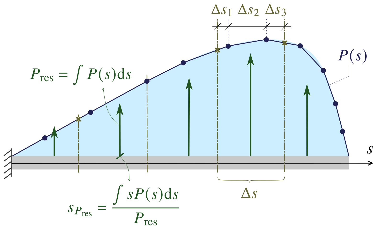
Figure 2 Calculation of equivalent concentrated loads from the spanwise load distribution. s: coordinate along beam length. Δs: length of spanwise portion. (•): distributed load value at load calculation points. (×): linearly interpolated distributed load value at spanwise portions defined.

More specifically, the equivalent concentrated load at each spanwise portion Δs (see Fig. 2) is calculated as follows: the different load components are integrated by considering each sub-portion Δs_i (defined by the load calculation points within Δs) individually and applying the Gauss–Legendre quadrature rule, as

$$\begin{array}{}\text{(18)}& P_{\mathrm{res}}=\sum _{\mathrm{\Delta }{s}_i}\underset{s_i^{\mathrm{0}}}{\overset{s_i^{\mathrm{0}}+\mathrm{\Delta }{s}_i}{\int }}P\left(s\right)\mathrm{d}s=\sum _{\mathrm{\Delta }{s}_i}\left(\sum _j^{n_{\mathrm{Gauss}}}{w}_{j}P\left(s_j\right)\right),\end{array}$$

where w_j is the weight corresponding to Gauss point s_j and $s_i^{\mathrm{0}}$ is the starting point of each spanwise sub-portion Δs_i. A total of n_Gauss Gauss points are used, and the load at each Gauss point P(s_j) is computed by linear interpolation between the two closest load calculation points.

A similar procedure is followed to calculate the corresponding load application point but computing instead the first moment of area $S_{P_{\mathrm{r}}}$ of the resultant aerodynamic force distribution, considering only the in-plane components (i.e. excluding the axial force component), such that $P_{\mathrm{r}}\left(s\right)=\sqrt{P_{\mathrm{flap}}^{\mathrm{2}}\left(s\right)+P_{\mathrm{edge}}^{\mathrm{2}}\left(s\right)}$. This translates to

$$\begin{array}{}\text{(19)}& S_{P_{\mathrm{r}}}=\sum _{\mathrm{\Delta }{s}_i}\underset{s_i^{\mathrm{0}}}{\overset{s_i^{\mathrm{0}}+\mathrm{\Delta }{s}_i}{\int }}s{P}_{\mathrm{r}}\left(s\right)\mathrm{d}s=\sum _{\mathrm{\Delta }{s}_i}\left(\sum _j^{n_{\mathrm{Gauss}}}{w}_j{s}_j{P}_{\mathrm{r}}\left(s_j\right)\right),\end{array}$$

from which the load application point can be calculated as $s_{P_{\mathrm{res}}}=S_{P_{\mathrm{r}}}/P_{\mathrm{res}}$. Since a linear load distribution P(s) is considered, two Gauss points (n_Gauss=2) are sufficient to yield an exact result for Eq. (19).

The concentrated loads calculated this way are applied to the model using interpolation multipoint constraints (RBE3). These couple the motion of a group of nodes to that of a main node R, such that the main node follows the weighted average motion of the n_c coupling nodes defined. Its (global) position ${\mathit{r}}_{\mathrm{R}}\in {\mathbb{R}}^{\mathrm{3}\times \mathrm{1}}$ is thus calculated as

$$\begin{array}{}\text{(20)}& {\mathit{r}}_{\mathrm{R}}={\mathit{q}}_{\mathrm{t}}+\mathbf{A}{\stackrel{\mathrm{‾}}{\mathit{r}}}_{{\mathrm{f}}_{\mathrm{R}}}\text{with}{\stackrel{\mathrm{‾}}{\mathit{r}}}_{{\mathrm{f}}_{\mathrm{R}}}=\sum _j^{n_{\mathrm{c}}}{w}_j\left({\stackrel{\mathrm{‾}}{\mathit{x}}}_j+{\stackrel{\mathrm{‾}}{\mathit{c}}}_{{\mathrm{f}}_j}\right),\end{array}$$

where w_j is the nodal weight attributed to coupling node j and ${\stackrel{\mathrm{‾}}{\mathit{x}}}_j,{\stackrel{\mathrm{‾}}{\mathit{c}}}_{{\mathrm{f}}_j}$ its local reference position and flexible displacement, respectively. Uniform nodal weights are used throughout this work. The local orientation ${\stackrel{\mathrm{‾}}{\mathit{\theta }}}_{{\mathrm{f}}_{\mathrm{R}}}\in {\mathbb{R}}^{\mathrm{3}\times \mathrm{1}}$ of the main node can be computed in different ways. In this work, the implementation of the object MarkerSuperElementRigid in Exudyn is adopted (Gerstmayr, 2025), which corresponds to

$$\begin{array}{}\text{(21)}& \begin{array}{rl}& {\stackrel{\mathrm{‾}}{\mathit{\theta }}}_{{\mathrm{f}}_{\mathrm{R}}}={\mathbf{W}}^{-\mathrm{1}}\sum _j^{n_{\mathrm{c}}}\left[w_j{\stackrel{\mathrm{̃}}{\stackrel{\mathrm{‾}}{\mathit{p}}}}_{j,\mathrm{R}}\left({\stackrel{\mathrm{‾}}{\mathit{c}}}_{{\mathrm{f}}_j}-\sum _i^{n_{\mathrm{c}}}{w}_i{\stackrel{\mathrm{‾}}{\mathit{c}}}_{{\mathrm{f}}_i}\right)\right]\\ & \text{with}{\stackrel{\mathrm{‾}}{\mathit{p}}}_{j,\mathrm{R}}={\stackrel{\mathrm{‾}}{\mathit{x}}}_j-\sum _j^{n_{\mathrm{c}}}{w}_j{\stackrel{\mathrm{‾}}{\mathit{x}}}_j,\end{array}\end{array}$$

where $\mathbf{W}=-{\sum }_j^{n_{\mathrm{c}}}{w}_j{\stackrel{\mathrm{‾}}{\mathit{p}}}_{j,\mathrm{R}}{\stackrel{\mathrm{‾}}{\mathit{p}}}_{j,\mathrm{R}}\in {\mathbb{R}}^{\mathrm{3}\times \mathrm{3}}$ represents the inertia tensor of the group of coupling nodes, considering that the nodal weights act as nodal masses. Note that ${\stackrel{\mathrm{‾}}{\mathit{\theta }}}_{{\mathrm{f}}_{\mathrm{R}}}$ is expressed in terms of the Cartesian rotation vector. The global orientation can be calculated as ${\mathbf{A}}_{\mathrm{R}}=\mathbf{A}\exp \left({\stackrel{\mathrm{̃}}{\stackrel{\mathrm{‾}}{\mathit{\theta }}}}_{{\mathrm{f}}_{\mathrm{R}}}\right)$, where exp (•) is the exponential map for SO(3).

Forces and moments applied at the main node $({\mathit{f}}_{\mathrm{R}},{\mathit{m}}_{\mathrm{R}}\in {\mathbb{R}}^{\mathrm{3}\times \mathrm{1}})$ are transmitted to the coupling nodes as applied nodal forces, which are then converted to generalised applied forces ${\widehat{\mathit{Q}}}_{{\mathrm{a}}_{\mathrm{c}}}$ as per Eqs. (15)–(17). This can be expressed as (Antunes et al., 2025b)

$$\begin{array}{}\text{(22)}& {\widehat{\mathit{Q}}}_{{\mathrm{a}}_{\mathrm{c}}}={\mathbf{J}}_{\mathrm{pos}}^{\top }{\mathit{f}}_{\mathrm{R}}+{\mathbf{J}}_{\mathrm{rot}}^{\top }{\mathit{m}}_{\mathrm{R}},\end{array}$$

where ${\mathbf{J}}_{\mathrm{pos}},{\mathbf{J}}_{\mathrm{rot}}\in {\mathbb{R}}^{\mathrm{3}\times (\mathrm{3}+n_{\mathrm{r}}+n_{\mathrm{f}})}$ are, respectively, the position and rotation Jacobians of the RBE3 multipoint constraint. Given the expressions above for the global position and orientation of the main node R, these correspond to (Gerstmayr, 2025; Antunes et al., 2025b)

$$\begin{array}{}\text{(23)}& {\displaystyle }{\mathbf{J}}_{\mathrm{pos}}& {\displaystyle }=\left[\begin{array}{ccc}\mathbf{I}& -\mathbf{A}{\stackrel{\mathrm{̃}}{\stackrel{\mathrm{‾}}{\mathit{r}}}}_{{\mathrm{f}}_{\mathrm{R}}}\stackrel{\mathrm{‾}}{\mathbf{G}}& \mathbf{A}\sum _j{w}_j{\stackrel{\mathrm{‾}}{\mathbf{\Psi }}}_{{\mathrm{rows}}_j}\end{array}\right],\text{(24)}& {\displaystyle }{\mathbf{J}}_{\mathrm{rot}}& {\displaystyle }=\left[\begin{array}{ccc}\mathbf{0}& \mathbf{A}\stackrel{\mathrm{‾}}{\mathbf{G}}& \mathbf{AT}\left({\stackrel{\mathrm{‾}}{\mathit{\theta }}}_{{\mathrm{f}}_{\mathrm{R}}}\right){\mathbf{W}}^{-\mathrm{1}}\sum _j{w}_j{\stackrel{\mathrm{̃}}{\stackrel{\mathrm{‾}}{\mathit{p}}}}_{j,\mathrm{R}}{\stackrel{\mathrm{‾}}{\mathbf{\Psi }}}_{{\mathrm{rows}}_j}\end{array}\right],\end{array}$$

with ${\stackrel{\mathrm{‾}}{\mathbf{\Psi }}}_{{\mathrm{rows}}_j}\in {\mathbb{R}}^{\mathrm{3}\times n_{\mathrm{f}}}$ representing the rows of the reduction basis relative to node j. T(•) is the tangent operator for SO(3).

For each concentrated load, the group of coupling nodes consists of all nodes belonging to the corresponding spanwise cross-section; the full cross-section nodes are chosen here, as opposed to all nodes belonging to each blade portion (Forcier and Joncas, 2020) or the spar cap nodes only (Bottasso et al., 2014; Haselbach et al., 2022), mainly for computational efficiency reasons (it leads to a smaller number of multipoint constraint equations than considering the whole blade portion) and simplicity of implementation (choosing only the spar cap nodes limits generalisation and makes the approach structure dependent). Although not demonstrated here, it is found that these different choices for defining the coupling nodes group generally yield similar results.

By following the above method, it is possible to apply multiple concentrated loads to this model that provide equivalent loading conditions to the aerodynamic load distribution computed by the aerodynamic solver. However, the cross-sections at which these are to be applied do not necessarily coincide with the substructuring interfaces (B0 and B1, see Fig. 1) defined for each sub-body of the multibody structure representing the wind turbine blade. Having an interface at the load application points is ideal, since it fulfils the Hurty/Craig-Bampton method assumption of external loads only being applied at interfaces, but that is not possible with the current approach: the number of sub-bodies should be as large as required to obtain a response converged to the nonlinear solution but not larger for computational efficiency reasons. The number of load application points will therefore likely be larger than the number of interfaces and will not be placed at the same locations.

There are two options to implement this load application method in the model: the simplest one consists of applying the loads at internal DOFs and projecting them onto the reduction basis subspace as per Eq. (17); the alternative is to include additional (internal) interfaces in each sub-body at the load application cross-sections.

Internal load interfaces can be included by considering the DOFs of the load application cross-sections as interface DOFs in the Hurty/Craig-Bampton method and calculating interface modes not only for the substructuring interfaces (B0, B1) but also for each load interface; these are then added to the block-diagonal interface reduction matrix in Eq. (12). The system size is increased by $n_{\mathrm{BL}}\cdot n_{{\mathrm{m}}_b}$ by doing this, depending on the number of load interfaces (n_BL).

Since these internal interfaces are added just for load application purposes, there is no need to have a large number of interface modes describing them. However, if the minimum number of six interface modes is used, the load interfaces will behave like rigid (RBE2) interfaces and introduce artificial stiffening in the system (Antunes et al., 2025b). To avoid this but still keep the number of DOFs per load interface to a minimum, one could instead use RBE3 interfaces. However, it is important that interface modes are kept for the substructuring interfaces of each sub-body, because the use of RBE3 interfaces to connect sub-bodies has been found to result in overly flexible structures with poor convergence properties.

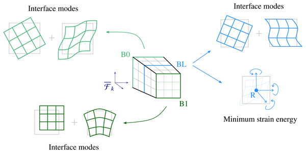
RBE3 multipoint constraints define the motion of the reference node as the weighted average of the motion from the coupling nodes. This is the opposite of a rigid (RBE2) constraint, in which the motion of the coupling nodes follows the rigid body motion of the reference node (Ahn et al., 2020). For this reason, it is not possible to express an RBE3 constraint in the form ${\stackrel{\mathrm{‾}}{\mathit{c}}}_{{\mathrm{f}}_b}={\stackrel{\mathrm{‾}}{\mathbf{\Psi }}}_b{\mathit{\zeta }}_b$ and, consequently, incorporate it in the interface reduction matrix together with ${\stackrel{\mathrm{‾}}{\mathbf{\Psi }}}_{b,\mathrm{B}\mathrm{0}}$ and ${\stackrel{\mathrm{‾}}{\mathbf{\Psi }}}_{b,\mathrm{B}\mathrm{1}}$, computed with interface modes. An analogous formulation developed by Masarati et al. (2020) is therefore used, which is further explained below. Figure 3 summarises the different interface reduction strategies used for each sub-body when internal load interfaces are considered.

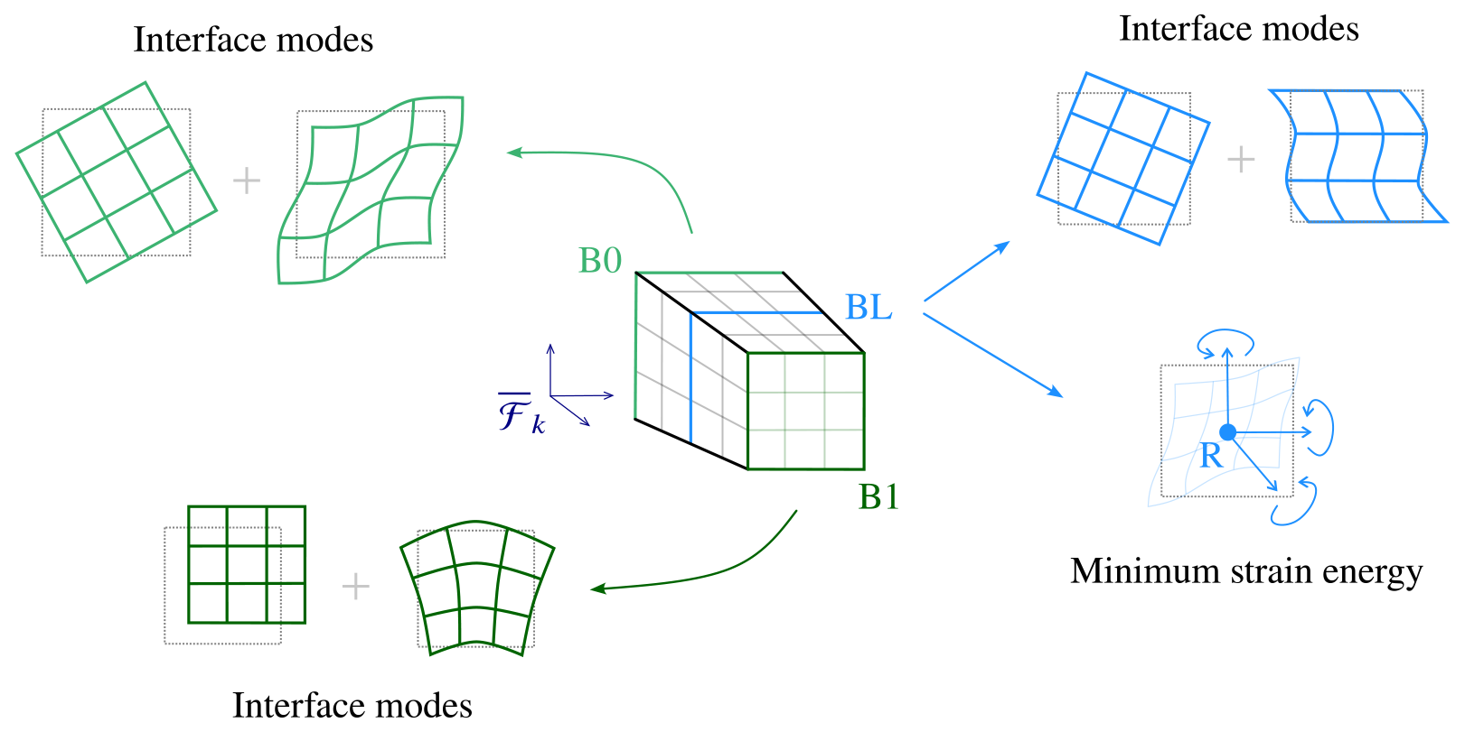
Figure 3 Interface reduction methods used for substructuring interfaces (B0, B1) and internal load interfaces (BL).

3.1.1 Minimum strain energy interfaces

The formulation developed by Masarati et al. (2020) starts from the decomposition of the interface node motion into a rigid body motion and a deformation motion, described by block-diagonal matrices $\stackrel{\mathrm{‾}}{\mathbf{H}}$ and $\stackrel{\mathrm{‾}}{\mathbf{C}}$, respectively:

$$\begin{array}{}\text{(25)}& {\stackrel{\mathrm{‾}}{\mathit{c}}}_{{\mathrm{f}}_b}=\stackrel{\mathrm{‾}}{\mathbf{H}}{\mathit{\zeta }}_{\mathrm{R}}+\stackrel{\mathrm{‾}}{\mathbf{C}}{\mathit{\zeta }}_{\mathrm{d}}.\end{array}$$

For each interface BX, the rigid body motion of the interface nodes is a function of the motion of point R located at the weighted average position of the interface nodes, described by generalised coordinates ${\mathit{\zeta }}_{\mathrm{R},\mathrm{BX}}\in {\mathbb{R}}^{\mathrm{6}\times \mathrm{1}}$ (representing the three displacements and three rotations of point R), and matrix ${\stackrel{\mathrm{‾}}{\mathbf{H}}}_{\mathrm{BX}}\in {\mathbb{R}}^{\mathrm{3}{n}_{\mathrm{BX}}\times \mathrm{6}}$, given by

$$\begin{array}{}\text{(26)}& {\stackrel{\mathrm{‾}}{\mathbf{H}}}_{\mathrm{BX}}=\left[\begin{array}{cc}\mathbf{I}& -{\stackrel{\mathrm{̃}}{\stackrel{\mathrm{‾}}{\mathit{p}}}}_{\mathrm{BX}}\end{array}\right]\text{with}{\stackrel{\mathrm{‾}}{\mathit{p}}}_{j,\mathrm{BX}}={\stackrel{\mathrm{‾}}{\mathit{x}}}_{j,\mathrm{BX}}-{\stackrel{\mathrm{‾}}{\mathit{x}}}_{\mathrm{R},\mathrm{BX}},\end{array}$$

where ${\stackrel{\mathrm{̃}}{\stackrel{\mathrm{‾}}{\mathit{p}}}}_{\mathrm{BX}}$ contains the stacked skew-symmetric matrices of the relative nodal reference positions of each interface node j relative to point R, ${\stackrel{\mathrm{‾}}{\mathit{p}}}_{j,\mathrm{BX}}\in {\mathbb{R}}^{\mathrm{3}\times \mathrm{1}}$.

The deformation motion is described by ${\stackrel{\mathrm{‾}}{\mathbf{C}}}_{\mathrm{BX}}\in {\mathbb{R}}^{\mathrm{3}{n}_{\mathrm{BX}}\times (\mathrm{3}{n}_{\mathrm{BX}}-\mathrm{6})}$, the complement to the rigid body matrix ${\stackrel{\mathrm{‾}}{\mathbf{H}}}_{\mathrm{BX}}$, which is, by definition, orthogonal to this matrix ${\stackrel{\mathrm{‾}}{\mathbf{C}}}^{\top }\stackrel{\mathrm{‾}}{\mathbf{H}}=\mathbf{0}$. Matrix ${\stackrel{\mathrm{‾}}{\mathbf{C}}}_{\mathrm{BX}}$ represents the warping of the interface relative to the rigid body motion, and the generalised coordinates ${\mathit{\zeta }}_{\mathrm{d},\mathrm{BX}}\in {\mathbb{R}}^{(\mathrm{3}{n}_{\mathrm{BX}}-\mathrm{6})\times \mathrm{1}}$ are the multiplication factors for these warping shapes. This matrix can be obtained from the QR decomposition of ${\stackrel{\mathrm{‾}}{\mathbf{H}}}_{\mathrm{BX}}$: matrix ${\stackrel{\mathrm{‾}}{\mathbf{C}}}_{\mathrm{BX}}$ will correspond to matrix Q₂.

A minimum strain energy interface is obtained by enforcing that no virtual work is done by the interface forces ${\stackrel{\mathrm{‾}}{\mathit{f}}}_{\mathrm{b}}$ for the subspace of the interface warping motion, i.e. ${\stackrel{\mathrm{‾}}{\mathbf{C}}}^{\top }{\stackrel{\mathrm{‾}}{\mathit{f}}}_b=\mathbf{0}$. By applying the principle of virtual work to the expression for the static virtual work at the interface $\mathit{\delta }{W}_{{\mathrm{s}}_b}$, which is given by (Masarati et al., 2020)

$$\begin{array}{}\text{(27)}& \begin{array}{rl}{\displaystyle }\mathit{\delta }{W}_{{\mathrm{s}}_b}& {\displaystyle }=\mathit{\delta }{W}_{\mathrm{s},{\mathrm{ext}}_b}+\mathit{\delta }{W}_{\mathrm{s},{\mathrm{int}}_b}\\ {\displaystyle }& {\displaystyle }={\left(\mathit{\delta }{\stackrel{\mathrm{‾}}{\mathit{c}}}_{{\mathrm{f}}_b}\right)}^{\top }{\stackrel{\mathrm{‾}}{\mathit{f}}}_b+{\left(\mathit{\delta }{\stackrel{\mathrm{‾}}{\mathit{c}}}_{{\mathrm{f}}_b}\right)}^{\top }{\stackrel{\mathrm{‾}}{\mathbf{K}}}_{{\mathrm{HCB}}_{bb}}{\stackrel{\mathrm{‾}}{\mathit{c}}}_{{\mathrm{f}}_b}\\ {\displaystyle }& {\displaystyle }={\left(\stackrel{\mathrm{‾}}{\mathbf{H}}{\mathit{\zeta }}_{\mathrm{R}}+\stackrel{\mathrm{‾}}{\mathbf{C}}{\mathit{\zeta }}_{\mathrm{d}}\right)}^{\top }\left[{\stackrel{\mathrm{‾}}{\mathit{f}}}_b+{\stackrel{\mathrm{‾}}{\mathbf{K}}}_{{\mathrm{HCB}}_{bb}}\left(\stackrel{\mathrm{‾}}{\mathbf{H}}{\mathit{\zeta }}_{\mathrm{R}}+\stackrel{\mathrm{‾}}{\mathbf{C}}{\mathit{\zeta }}_{\mathrm{d}}\right)\right],\end{array}\end{array}$$

two equations are obtained:

$$\begin{array}{}\text{(28)}& {\displaystyle }{\stackrel{\mathrm{‾}}{\mathbf{H}}}^{\top }{\stackrel{\mathrm{‾}}{\mathit{f}}}_b-{\stackrel{\mathrm{‾}}{\mathbf{H}}}^{\top }{\stackrel{\mathrm{‾}}{\mathbf{K}}}_{{\mathrm{HCB}}_{bb}}\stackrel{\mathrm{‾}}{\mathbf{H}}{\mathit{\zeta }}_{\mathrm{R}}-{\stackrel{\mathrm{‾}}{\mathbf{H}}}^{\top }{\stackrel{\mathrm{‾}}{\mathbf{K}}}_{{\mathrm{HCB}}_{bb}}\stackrel{\mathrm{‾}}{\mathbf{C}}{\mathit{\zeta }}_{\mathrm{d}}& {\displaystyle }=\mathbf{0},\text{(29)}& {\displaystyle }{\stackrel{\mathrm{‾}}{\mathbf{C}}}^{\top }{\stackrel{\mathrm{‾}}{\mathit{f}}}_b-{\stackrel{\mathrm{‾}}{\mathbf{C}}}^{\top }{\stackrel{\mathrm{‾}}{\mathbf{K}}}_{{\mathrm{HCB}}_{bb}}\stackrel{\mathrm{‾}}{\mathbf{H}}{\mathit{\zeta }}_{\mathrm{R}}-{\stackrel{\mathrm{‾}}{\mathbf{C}}}^{\top }{\stackrel{\mathrm{‾}}{\mathbf{K}}}_{{\mathrm{HCB}}_{bb}}\stackrel{\mathrm{‾}}{\mathbf{C}}{\mathit{\zeta }}_{\mathrm{d}}& {\displaystyle }=\mathbf{0},\end{array}$$

where ${\stackrel{\mathrm{‾}}{\mathbf{K}}}_{{\mathrm{HCB}}_{bb}}$ is the portion of the Hurty/Craig-Bampton reduced stiffness matrix relative to the retained interface DOFs. Applying the minimum strain energy interface condition to Eq. (29) allows one to express the warping motion of the interface, represented by the generalised coordinates ζ_d, as a function of the rigid body generalised coordinates ζ_R only, as

$$\begin{array}{}\text{(30)}& {\mathit{\zeta }}_{\mathrm{d}}=-{\left({\stackrel{\mathrm{‾}}{\mathbf{C}}}^{\top }{\stackrel{\mathrm{‾}}{\mathbf{K}}}_{{\mathrm{HCB}}_{bb}}\stackrel{\mathrm{‾}}{\mathbf{C}}\right)}^{-\mathrm{1}}{\stackrel{\mathrm{‾}}{\mathbf{C}}}^{\top }{\stackrel{\mathrm{‾}}{\mathbf{K}}}_{{\mathrm{HCB}}_{bb}}\stackrel{\mathrm{‾}}{\mathbf{H}}{\mathit{\zeta }}_{\mathrm{R}}.\end{array}$$

The final interface reduction basis is obtained by substituting Eq. (30) into Eq. (25):

$$\begin{array}{}\text{(31)}& \begin{array}{rl}{\stackrel{\mathrm{‾}}{\mathbf{\Psi }}}_{b,\mathrm{MSE}}& =\stackrel{\mathrm{‾}}{\mathbf{P}}\stackrel{\mathrm{‾}}{\mathbf{H}}\text{with}\\ \stackrel{\mathrm{‾}}{\mathbf{P}}& =\mathbf{I}-\stackrel{\mathrm{‾}}{\mathbf{C}}{\left({\stackrel{\mathrm{‾}}{\mathbf{C}}}^{\top }{\stackrel{\mathrm{‾}}{\mathbf{K}}}_{{\mathrm{HCB}}_{bb}}\stackrel{\mathrm{‾}}{\mathbf{C}}\right)}^{-\mathrm{1}}{\stackrel{\mathrm{‾}}{\mathbf{C}}}^{\top }{\stackrel{\mathrm{‾}}{\mathbf{K}}}_{{\mathrm{HCB}}_{bb}}.\end{array}\end{array}$$

This formulation is presented as being analogous to an RBE3 multipoint constraint, with the difference that the equivalent rigid body motion of main node R is not solely based on geometric considerations but rather on the static equilibrium condition at the interface.

To use this formulation as an alternative interface reduction method for the internal load interfaces (while keeping the interface modes for the substructuring interfaces of each sub-body), the below steps should be followed:

1. Compute the Hurty/Craig-Bampton reduced matrices (${\stackrel{\mathrm{‾}}{\mathbf{K}}}_{\mathrm{HCB}},{\stackrel{\mathrm{‾}}{\mathbf{M}}}_{\mathrm{HCB}}$) considering only the substructuring interfaces B0 and B1 as interface DOFs.

2. Compute the interface mode reduction matrices for the substructuring interfaces ${\stackrel{\mathrm{‾}}{\mathbf{\Psi }}}_{b,\mathrm{B}\mathrm{0}}$ and ${\stackrel{\mathrm{‾}}{\mathbf{\Psi }}}_{b,\mathrm{B}\mathrm{1}}$ using the reduced matrices from the previous step.

3. Compute the Hurty/Craig-Bampton reduced matrices considering only the load interfaces as interface DOFs.

4. Compute ${\stackrel{\mathrm{‾}}{\mathbf{\Psi }}}_{b,\mathrm{MSE}}$ for the load interfaces using the reduced matrices from the previous step.

5. Build the final interface reduction matrix:

   $$\begin{array}{}\text{(32)}& {\stackrel{\mathrm{‾}}{\mathbf{\Psi }}}_b=\left[\begin{array}{ccc}{\stackrel{\mathrm{‾}}{\mathbf{\Psi }}}_{b,\mathrm{B}\mathrm{0}}& \mathbf{0}& \mathbf{0}\\ \mathbf{0}& {\stackrel{\mathrm{‾}}{\mathbf{\Psi }}}_{b,\mathrm{MSE}}& \mathbf{0}\\ \mathbf{0}& \mathbf{0}& {\stackrel{\mathrm{‾}}{\mathbf{\Psi }}}_{b,\mathrm{B}\mathrm{1}}\end{array}\right].\end{array}$$

6. Update ${\stackrel{\mathrm{‾}}{\mathbf{\Psi }}}_{b,\mathrm{B}\mathrm{0}}$ and ${\stackrel{\mathrm{‾}}{\mathbf{\Psi }}}_{b,\mathrm{B}\mathrm{1}}$ in the final interface reduction matrices of each sub-body based on the common interface modes bases, calculated using SVD between adjacent sub-bodies.

7. Compute the Hurty/Craig-Bampton reduction matrix ${\stackrel{\mathrm{‾}}{\mathbf{\Psi }}}_{\mathrm{HCB}}$ considering all interface DOFs (B0, B1 and load interfaces).

8. Compute the final reduction matrix using Eq. (13) and ${\stackrel{\mathrm{‾}}{\mathbf{\Psi }}}_{\mathrm{HCB}}$ from the previous step.

It should be noted that different Hurty/Craig-Bampton reduced matrices are used in the calculation of the interface modes and minimum strain energy interface reduction matrices. This is needed to ensure that all six rigid body modes are included in the interface mode basis of B0 and B1, which is not the case if the Hurty/Craig-Bampton reduction step is instead only performed once and the interface modes are calculated using the portions from ${\stackrel{\mathrm{‾}}{\mathbf{K}}}_{\mathrm{HCB}},{\stackrel{\mathrm{‾}}{\mathbf{M}}}_{\mathrm{HCB}}$ relative to the interface DOFs belonging to B0 and B1.

4 Results

The nonlinear static analysis of two cantilever structures is presented. In Sect. 4.1, a simple isotropic beam is studied with the objective of answering the two main questions related to the load application methodology presented: first, how accurately can equivalent concentrated loads represent the loading conditions of an actual distributed load (Sect. 4.1.1)? Second, what is the impact of applying concentrated loads in the internal DOFs of the FFRF-based reduced-order model studied (Sect. 4.1.2)? The different options to achieve the latter (i.e. including or not including internal load interfaces, modelled with interface modes or minimum strain energy interfaces) are investigated. In Sect. 4.2, this methodology is applied to an actual wind turbine blade, subjected to an aerodynamic load distribution obtained from a steady state analysis.

The static response computed by the FFRF-based reduced-order model from solid elements implemented in Exudyn is compared with the reference solution from the original solid FE model, created in Abaqus (Dassault Systèmes, 2023). HAWC2 is also included in the comparison as an analogous FFRF-based model using beam elements, extensively used in wind energy research and industry. The models in Exudyn are generated from the mass and stiffness matrices of the solid FE model, exported from Abaqus. The cross-sectional properties of the beam in HAWC2 are computed using BECAS v4.0 (Blasques, 2012), which needs as input two-dimensional models of the cross-sections: for the isotropic beam, these are created in Abaqus; for the wind turbine blade, the aerostructural optimisation framework for wind turbine design (AESOpt) (Zahle et al., 2024) is used. This framework interfaces with BECAS and creates the cross-sectional meshes of each blade section using the properties described with the WindIO wind turbine ontology (Bortolotti et al., 2022).

The static response is compared in terms of the global displacement and rotation (rotation vector) components computed by the different models. For the models implemented in Abaqus and Exudyn, the rotation corresponds to an average quantity calculated using the Kabsch algorithm (Kabsch, 1978) for selected cross-sections; for the HAWC2 beam model, the nodal rotation values are used directly. The same global coordinate system is adopted in both structures analysed, with the x axis along the cross-section width/chord (lateral direction), the y axis along the cross-section height (transverse direction) and the z axis along the beam span (axial direction).

The system size is used in the analysis as a measure of computational cost. For the FFRF-based models, it is calculated as the sum of the number of DOFs belonging to each sub-body (FF and flexible generalised coordinates) and the number of algebraic equations (constraint equations) needed to define the boundary and reference conditions, as well as connecting the sub-bodies.

4.1 Isotropic beam

The structure analysed here is an isotropic beam of square cross-section (0.5×0.5 m) and length of 25 m. It is characterised by a Young's modulus of 2.6×10⁷ Pa and a Poisson's ratio of 0.3.

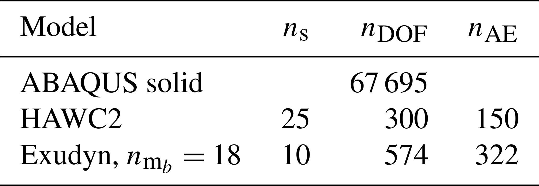
The system size of the models compared is shown in Table 1 and defined based on convergence studies. The reference Abaqus FE model is composed of 4000 solid elements of type C3D20R (quadratic brick elements with reduced integration) (Dassault Systèmes, 2023). Since only the static response is analysed, no fixed-interface eigenmodes are included in the Hurty/Craig-Bampton reduction step of the Exudyn reduced-order models ($n_{{\mathrm{m}}_i}=\mathrm{0}$); the baseline number of interface modes ($n_{{\mathrm{m}}_b}$) is 18. In the HAWC2 beam model, one element per sub-body is considered.

The models and results presented in this section are available from Antunes (2025).

Table 1 System size of isotropic beam models. n_s: number of sub-bodies, n_DOF: number of degrees of freedom, n_AE: number of algebraic equations.

4.1.1 Distributed triangular surface load

The first load case consists of a distributed triangular surface load, described by q(z)=2.4z [N m⁻²], such that its magnitude increases from zero at the clamped location to q=60 N m⁻² at the tip. It is applied at the middle surface of the beam with a fixed direction $\mathit{n}=\left[\begin{array}{ccc}\mathrm{0}& -\mathrm{1}& \mathrm{0}\end{array}\right]$.

There are two different ways to model this load in Abaqus: by integrating it over the deformed surface area (i.e. integration is carried out on the current configuration in each load step) or over the reference surface area, which corresponds to having a constant resultant load (integration is only performed once and the nodal load vector is maintained constant during the solution procedure) (Dassault Systèmes, 2023). The first option is the one that better represents a wind load.

To assess how accurately multiple concentrated loads can produce the same nonlinear static response as that of the actual distributed load, the reference Abaqus solid FE model was simulated with different loading conditions: with the distributed load integrated over the deformed surface area (reference solution), with the distributed load integrated over the reference surface area ($F_{\mathrm{res}}=\mathrm{const}.$) and with a different number of concentrated loads. The equivalent concentrated loads are calculated as described in Sect. 3.1: the beam is divided into equal spanwise portions, for which the resultant loads and corresponding load application points are calculated using Gauss–Legendre quadrature.

The static displacements and rotations computed with the different loading conditions are shown in Fig. 4, and the absolute and relative differences w.r.t. the Abaqus solution for the distributed load integrated over the deformed surface area can be seen in Fig. 5. There is a difference of around 3.5 % for the transverse displacement (u_y) and 7.5 % for the axial displacement (u_z) between the two distributed load solutions; this is expected for such large deflections.

The static response produced by the equivalent concentrated loads can only match that of the distributed load integrated over the reference area ($F_{\mathrm{res}}=\mathrm{const}.$), which is what is observed in these results. Consequently, a certain error is always present when using equivalent concentrated loads to emulate distributed loads, since these are not recalculated as the structure deforms; this error increases with the deflection magnitude. It should be remembered that the current approach allows for the modelling of follower loads (i.e. the load direction can be updated as the structure deforms). However, since the deformed orientation is only assessed at the discrete load application points, this may also constitute a small additional source of error when follower loads are simulated.

As the number of concentrated loads is increased, the static response converges to that of the distributed load (with $F_{\mathrm{res}}=\mathrm{const}.$). In fact, only a small number of load points is required to achieve an identical response to the one produced by the distributed load in question, with a difference lower than 1 % between the multiple solutions. Specifically, the maximum relative difference between the solution with five equivalent concentrated loads and the original distributed load is solely 0.6 %, and no differences are effectively observed when 50 equivalent concentrated loads are used.

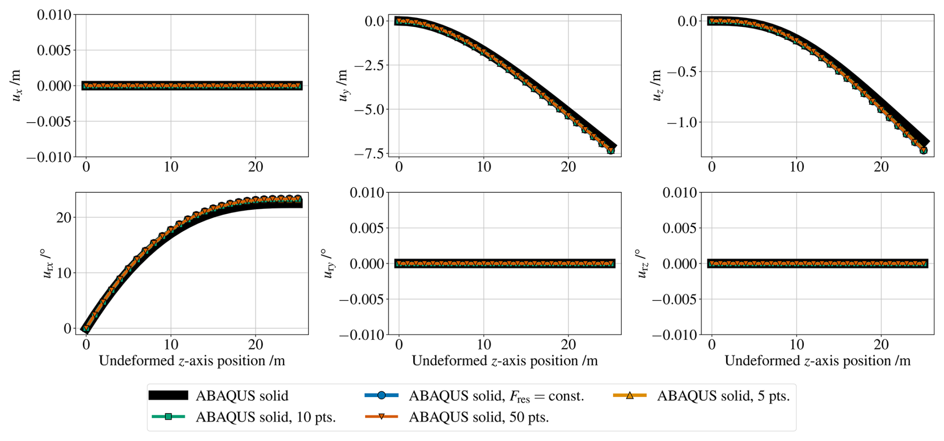
Figure 4 Isotropic beam subjected to distributed triangular load: comparison of the static displacement and rotation (rotation vector) components computed by Abaqus using the actual distributed load or equivalent concentrated loads.

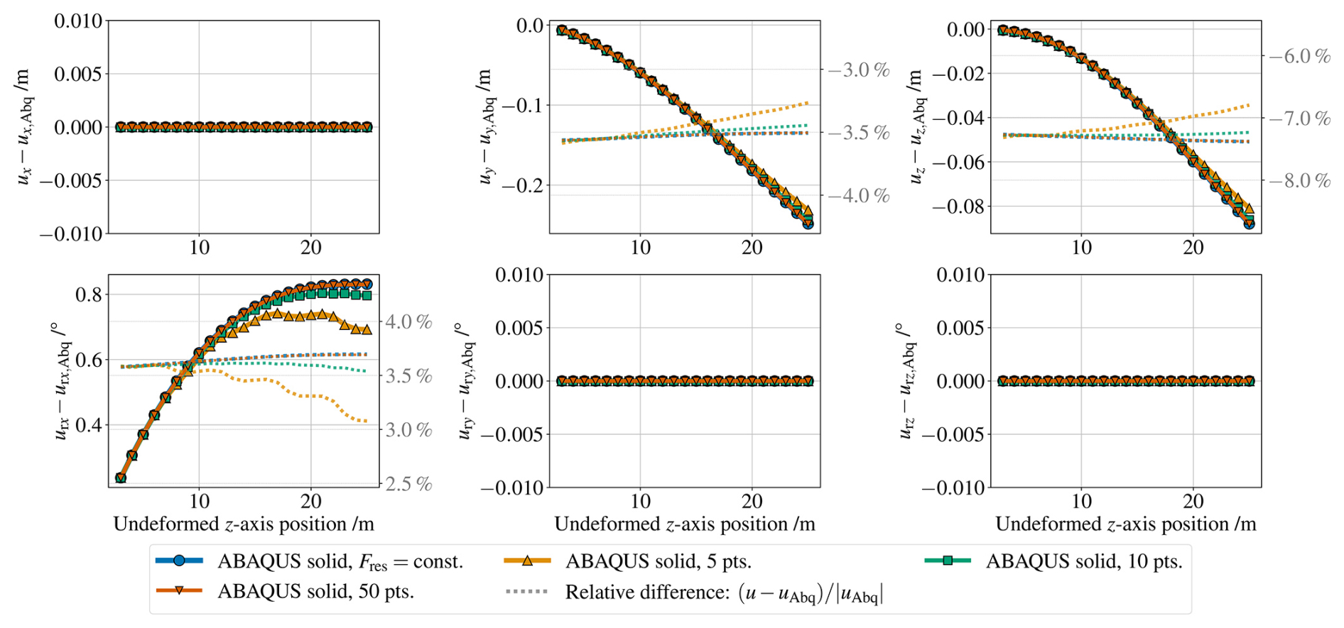
Figure 5 Isotropic beam subjected to distributed triangular load: absolute and relative differences of the displacement and rotation components computed by Abaqus using the actual distributed load or equivalent concentrated loads.

4.1.2 Multiple concentrated loads applied at internal DOFs

In this load case, multiple concentrated loads are applied at certain spanwise locations of the isotropic beam. The transverse forces are back-calculated from the theoretical bending moment distribution corresponding to the application of a triangular distributed load, such that a tip transverse deflection of about 20 % is obtained. The forces are assumed to be applied at the “quarter-chord” point of the cross-section, resulting in a torsional moment distribution as well. The load magnitudes and locations are given in Table 2.

Table 2 Concentrated loads applied to isotropic beam.

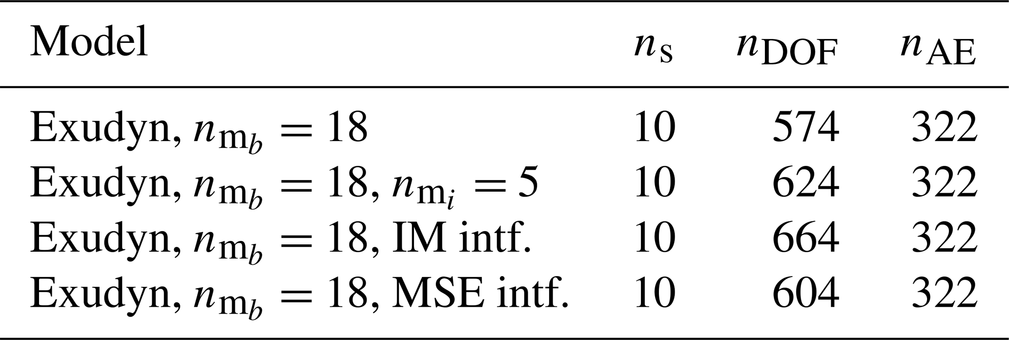
With this load case, the objective is to assess how the FFRF-based reduced-order models implemented in Exudyn handle the application of external loads at internal DOFs of sub-bodies. The baseline Exudyn model is the one referred to in Table 1, composed of 10 sub-bodies (each with a length of 2.5 m) generated with 18 interface modes. In this analysis, three alternative versions of this model are considered: one including a number of fixed-interface modes ($n_{{\mathrm{m}}_i}$) in the Hurty/Craig-Bampton reduction and two including internal load interfaces, using either interface modes (IMs) or minimum strain energy (MSE) interfaces. The reason behind the inclusion of internal load interfaces has been explained in Sect. 3.1 and relies on the assumption of the Hurty/Craig-Bampton method that external loads are only applied to interface DOFs. The inclusion of fixed-interface modes in this analysis aims at improving the basis these applied loads are projected onto – see Eq. (17) – especially when having torsional loads; a number of five fixed-interface modes is chosen to ensure that the first torsion mode is included in the reduction basis. The system size of these additional models considered in the analysis is displayed in Table 3.

Table 3 System size of Exudyn models used in the multiple concentrated loads test case (isotropic beam). n_s: number of sub-bodies, n_DOF: number of degrees of freedom, n_AE: number of algebraic equations.

The nonlinear static response computed by the different versions of the Exudyn models is compared with the reference solution from Abaqus and the HAWC2 beam model in Fig. 7. The corresponding absolute and relative differences w.r.t. the reference Abaqus model are shown in Fig. 8. A rendered view of the Exudyn solution for the baseline model is displayed in Fig. 6.

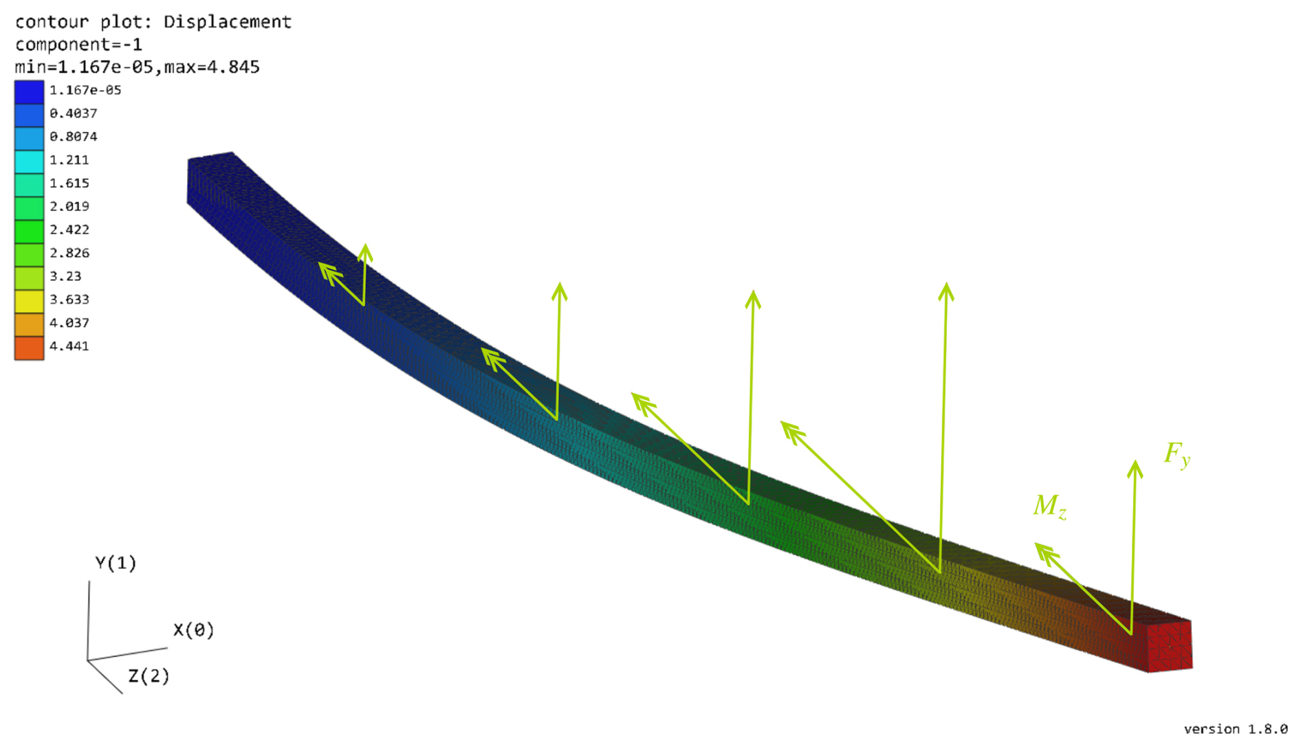
Figure 6 Rendered solution from Exudyn for isotropic beam subjected to multiple concentrated loads (baseline solution, $n_{{\mathrm{m}}_b}=\mathrm{18}$).

Overall, a good agreement is observed between all models, with the FFRF-based models (HAWC2 and the Exudyn models) showing similar relative differences w.r.t. the solid FE model from Abaqus, below 2 % for the majority of displacement and rotation components (with the exception of u_x and u_ry, which are components of smaller magnitude, with the maximum value of u_x corresponding to 0.3 % of the beam length).

When comparing the different versions of the Exudyn models, it is clear that the main challenge lies with the twist rotation component (u_rz), for which the baseline model shows a jump in the difference with respect to the reference solution around the load application points (see Fig. 8). Although the difference is small, it serves here to demonstrate the outcome of applying loads at internal DOFs. This difference is slightly lowered by including the torsion eigenmode ($n_{{\mathrm{m}}_i}=\mathrm{5}$) in the reduction matrix of the sub-bodies, while the inclusion of internal load interfaces (both with interface modes or minimum strain energy interfaces) eliminates these jumps. The best results amongst the Exudyn models are obtained with the model including interface mode load interfaces (IM intf.), but the gains are marginal when compared to the baseline model.

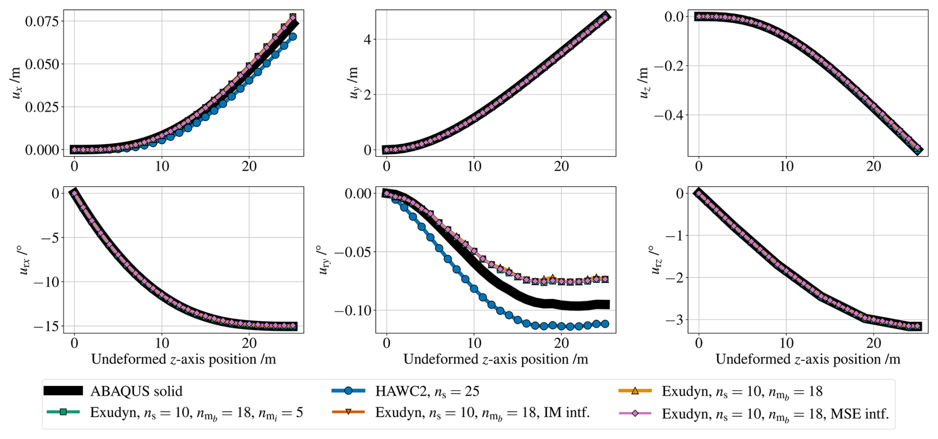
Figure 7 Isotropic beam subjected to multiple concentrated loads: comparison of the static displacement and rotation (rotation vector) components computed by the different models.

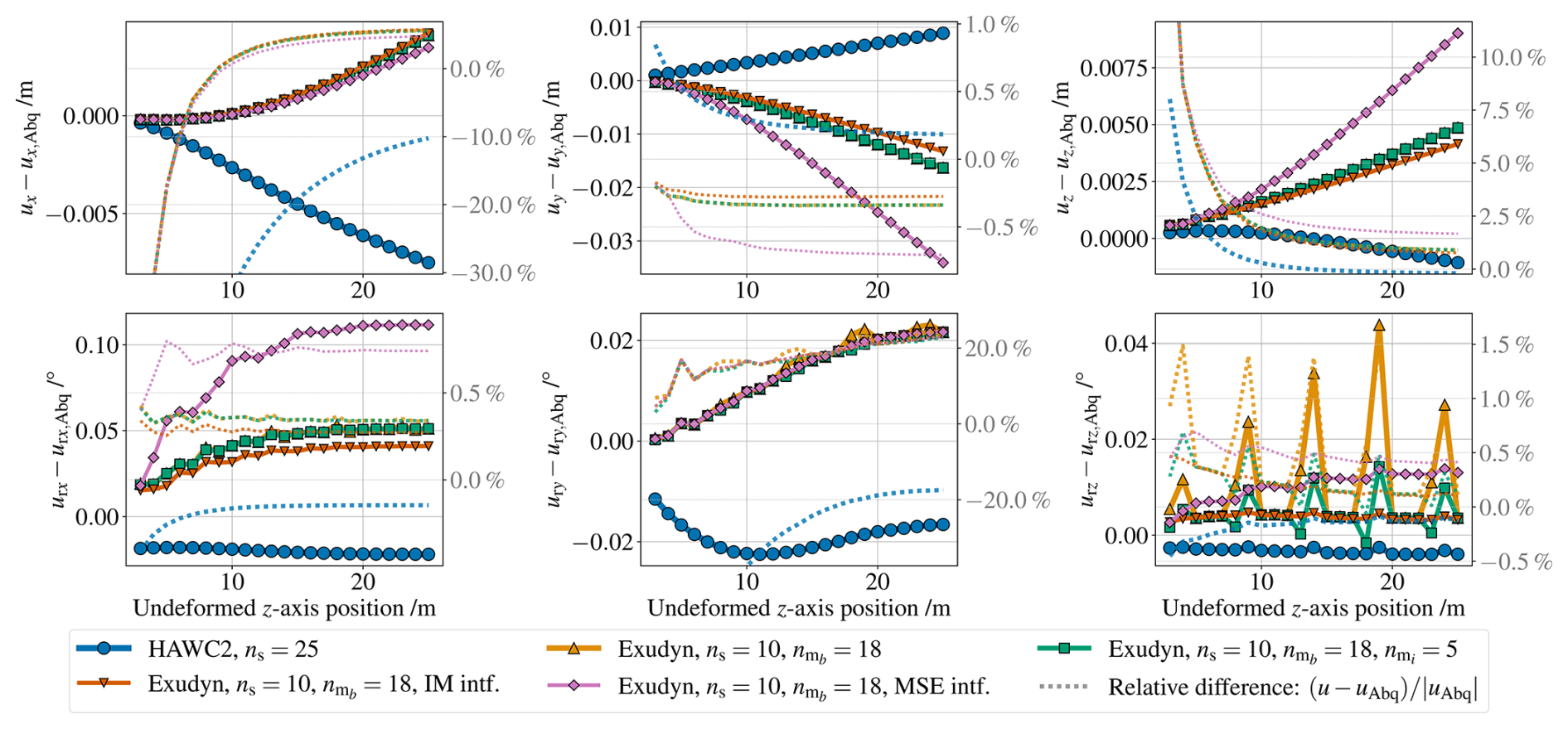
Figure 8 Isotropic beam subjected to multiple concentrated loads: absolute and relative differences of the displacement and rotation components w.r.t. the reference Abaqus solid FE model.

While the model with minimum strain energy load interfaces (MSE intf.) also resolves the issue of increased error in twist rotation around load application points, it exhibits a less-accurate response for the remaining deflection components when compared with the other Exudyn models. It computes a stiffer response, which is confirmed by the modal analysis performed on these models, shown in Fig. 9. Although this model constitutes an alternative with fewer DOFs than the model with interface modes load interfaces, it is not an ideal solution, as the response computed is not as accurate as the baseline Exudyn model. It also requires a greater preprocessing effort to build the reduced-order model, as detailed in Sect. 3.1.1.

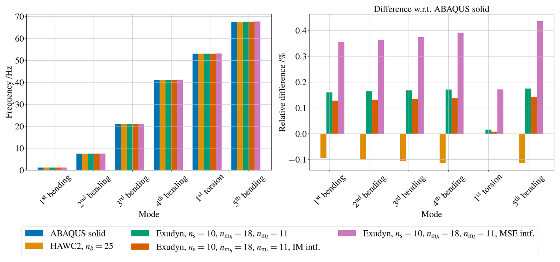
Figure 9 Isotropic beam: natural frequencies comparison. Relative differences calculated as $\left(f-f_{\mathrm{Abq}}\right)/f_{\mathrm{Abq}}$.

4.2 DTU 12.6 m wind turbine blade

The wind turbine blade analysed in this work has been designed and manufactured at DTU Wind and Energy Systems and is 12.6 m long (see Fig. 10). It does not fully represent the state of the art in modern pitch-regulated blades, as it was designed as a replacement for old 150 kW wind turbines, but it features the load-carrying shell concept, representative of current technology in terms of structural design (Haselbach et al., 2020a, b). It has been chosen due to the availability of a detailed structural (solid FE) model for a validated design, which is not provided for reference wind turbines at the present time. An analysis of this blade for similar loading conditions has been previously done in Antunes et al. (2024), including only the HAWC2 beam and high-fidelity FE models.

Figure 10 DTU 12.6 m wind turbine blade model. c: chord length.

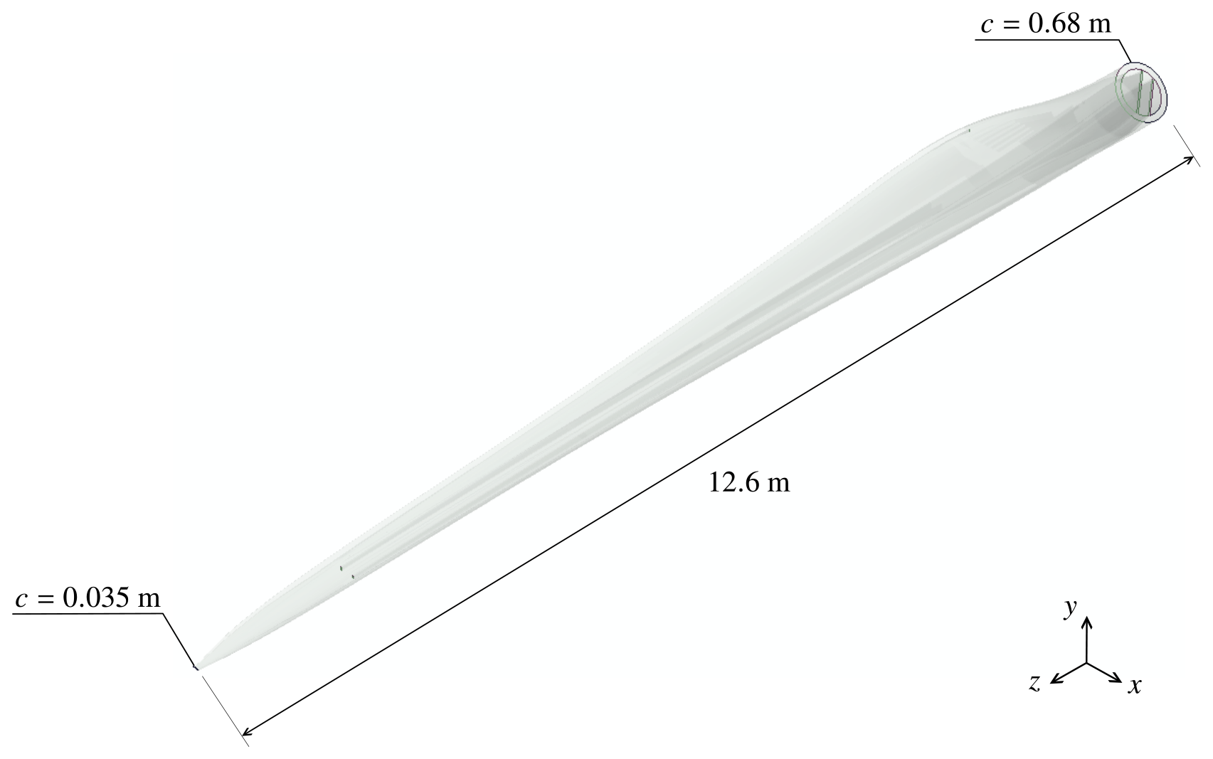
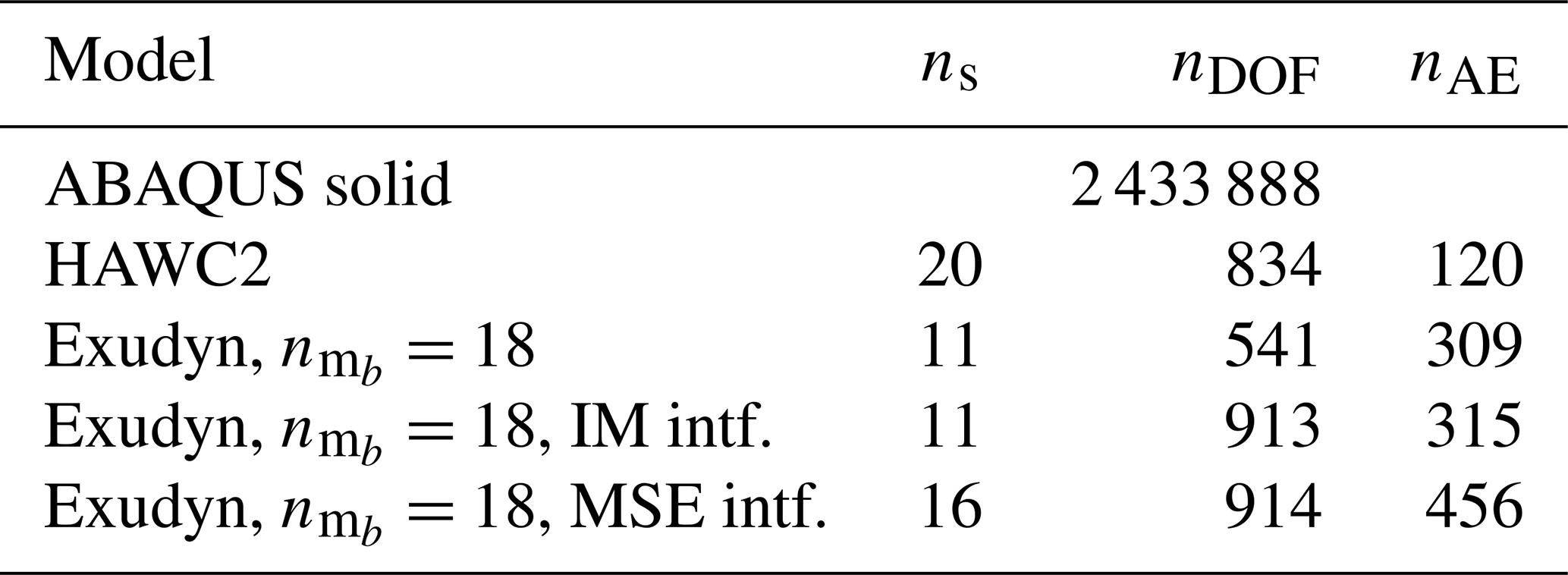
The system size of the models compared is shown in Table 4 and defined based on convergence studies. The reference Abaqus model is composed of 208 744 solid elements of type C3D8R (linear brick elements with reduced integration) (Dassault Systèmes, 2023). Similarly to the isotropic beam models, no fixed-interface modes are included in the Hurty/Craig-Bampton reduction matrix of the Exudyn models, which are generated with 18 interface modes. The HAWC2 beam model is composed of 119 elements, distributed by the defined number of sub-bodies.

Table 4 System size of DTU 12.6 m blade models. n_s: number of sub-bodies, n_DOF: number of degrees of freedom, n_AE: number of algebraic equations.

The loading conditions are based on the steady state aeroelastic analysis of the 150 kW wind turbine from Haselbach et al. (2020b). The aeroservoelastic stability analysis tool HAWCStab2 (Hansen et al., 2018; Hansen, 2004) is used to compute the distributed aerodynamic loads at rated wind speed (V_rat=12 m s⁻¹). The equivalent concentrated loads are calculated as described in Sect. 3.1 by integrating this aerodynamic load distribution over the blade length. Twenty load application points are considered, whose location is calculated from the distribution of the resultant in-plane forces (F_x,F_y), as described in Sect. 3.1. The original aerodynamic distributed loads and equivalent concentrated loads are plotted in Fig. 11. These are scaled by a factor of 4 in the current analysis, to be able to analyse geometrically nonlinear effects.

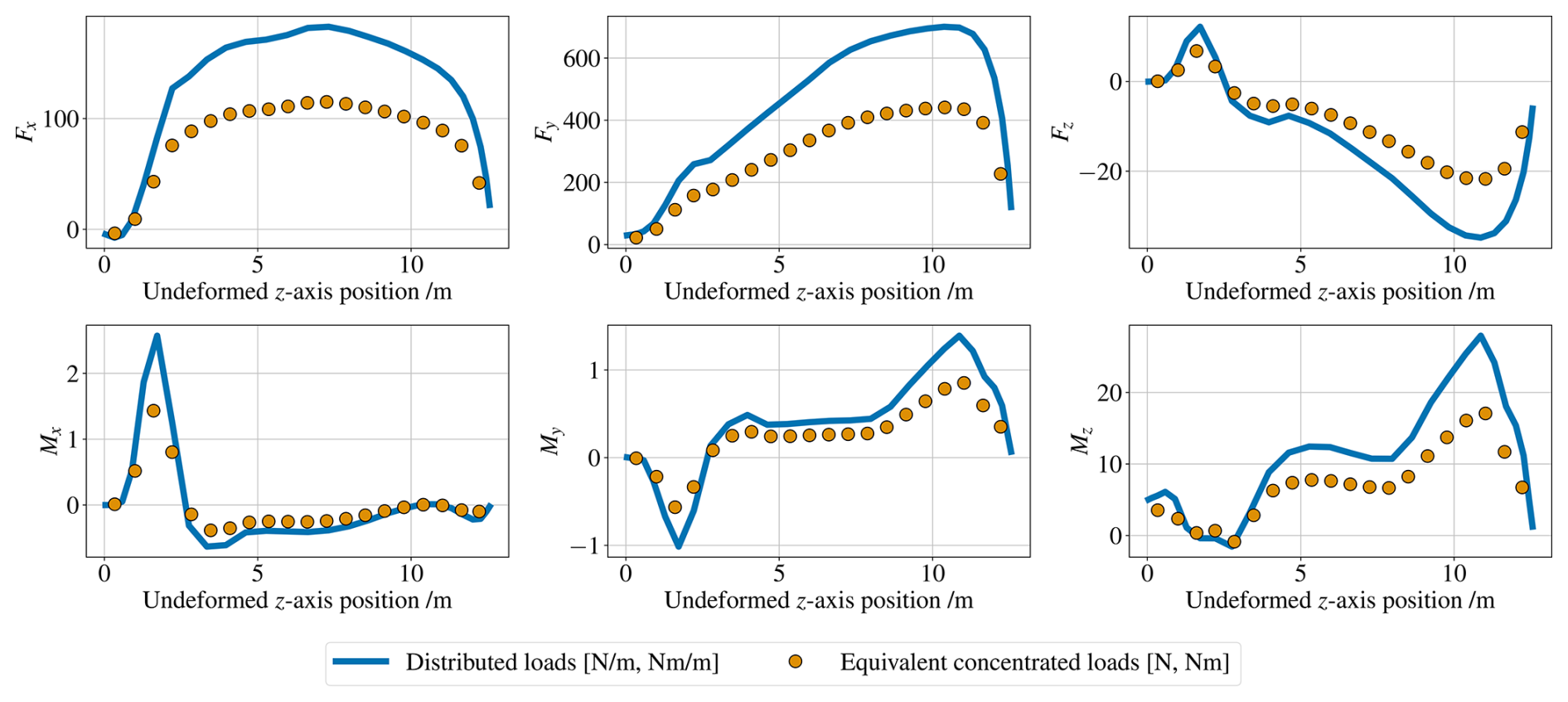
Figure 11 DTU 12.6 m blade: steady state distributed aerodynamic loads and calculated equivalent concentrated loads (unscaled). Loads are given at the elastic centre in the global coordinate system (z axis towards blade tip; x axis along blade root chordwise direction, towards leading edge; y axis towards blade root suction side).

The nonlinear static response to these loads, computed by the different models, is shown in Fig. 12, together with the absolute and relative differences w.r.t. the reference Abaqus solution in Fig. 13. It can be seen that the HAWC2 beam and Exudyn models including only interface modes (with and without load interfaces) are in close agreement with the Abaqus solid FE model, with all displacement and rotation components being within 1 %–3 % of the reference solution, with the exception of the torsion DOF (u_rz). This is not the case for the Exudyn model including minimum strain energy (MSE) interfaces, which again computes a stiffer response than the remaining models; for example, the transverse displacement is 5 % lower than the reference solution from Abaqus, while this difference is below 1 % for the other FFRF-based models.

The largest discrepancy in the HAWC2 model is observed for the twist rotation component, which does not exhibit the same behaviour as the Abaqus solid FE model. This is the consequence of abrupt structural variations in the model, in this case, changes in materials and the start/end of the shear webs in the blade, whose impact on the response is not as well captured by beam models, as these do not account for three-dimensional effects (Antunes et al., 2024). Since the FFRF-based reduced-order models implemented in Exudyn are based on the original solid FE model, they can capture better these complex structural phenomena, while still having a significantly smaller system size than a full three-dimensional FE model.

Finally, it should be noted that the difference between the static response computed by the baseline Exudyn model and the one including interface mode (IM) load interfaces is minimal. These results seem to indicate that there is no clear advantage in adding internal load interfaces to such reduced-order models for static analyses.

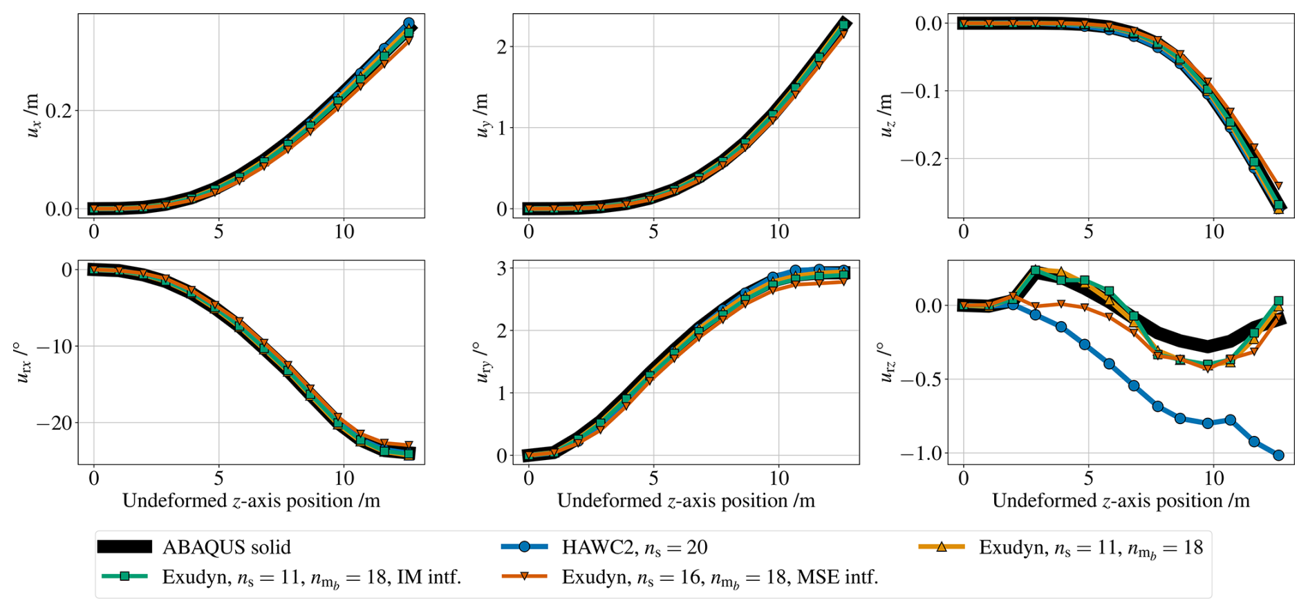
Figure 12 DTU 12.6 m blade: comparison of the static displacement and rotation (rotation vector) components computed by the different models.

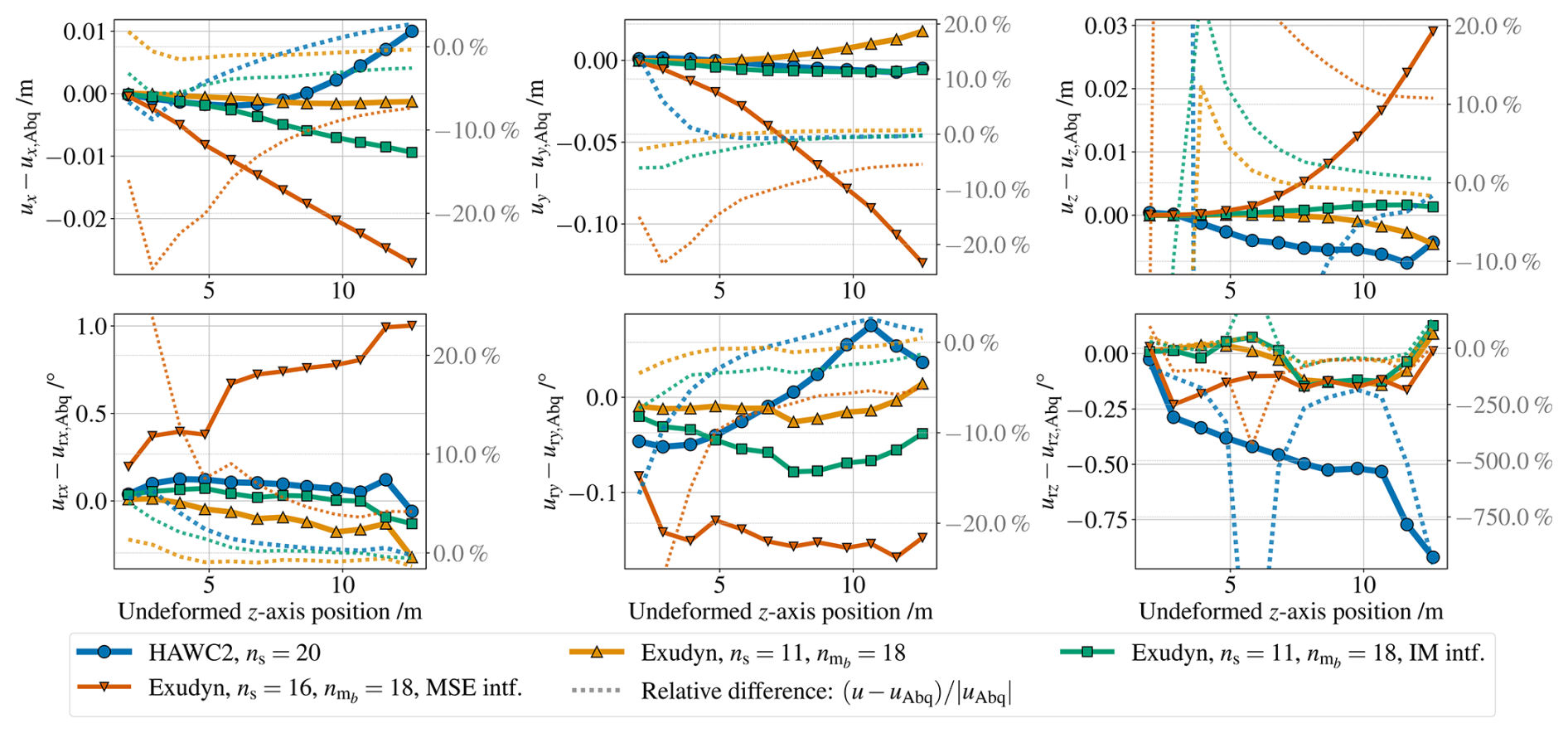
Figure 13 DTU 12.6 m blade: absolute and relative differences of the displacement and rotation components w.r.t. the reference Abaqus solid FE model.

To support the nonlinear static analysis, a modal analysis was also performed: the natural frequencies of the various models under investigation are presented in Fig. 14. The HAWC2 beam model considered in this study has a scaled mass distribution in order to match the total blade mass of the Abaqus solid FE model; this means that the original mass distribution (obtained from BECAS) is multiplied by a factor of 1.05. A total of eight fixed-interface modes is considered for the Exudyn models.

As previously observed for the isotropic beam model, the method including minimum strain energy (MSE) interfaces leads to a stiffer model. The natural frequencies of the other two Exudyn models are in complete agreement with the original Abaqus solid model, within 1 % for the baseline Exudyn model and within 1 %–3 % for the model including interface mode (IM) load interfaces. A good match is also noted between HAWC2 and Abaqus for all eigenmodes except for the first torsion mode, in which a large difference (above 20 %) is seen, confirming a well-known challenge in the modelling of wind turbine blades with beam models and highlighting the possible benefits of using the current reduced-order model based on solid finite elements (relative difference is below 1 % for the torsion mode).

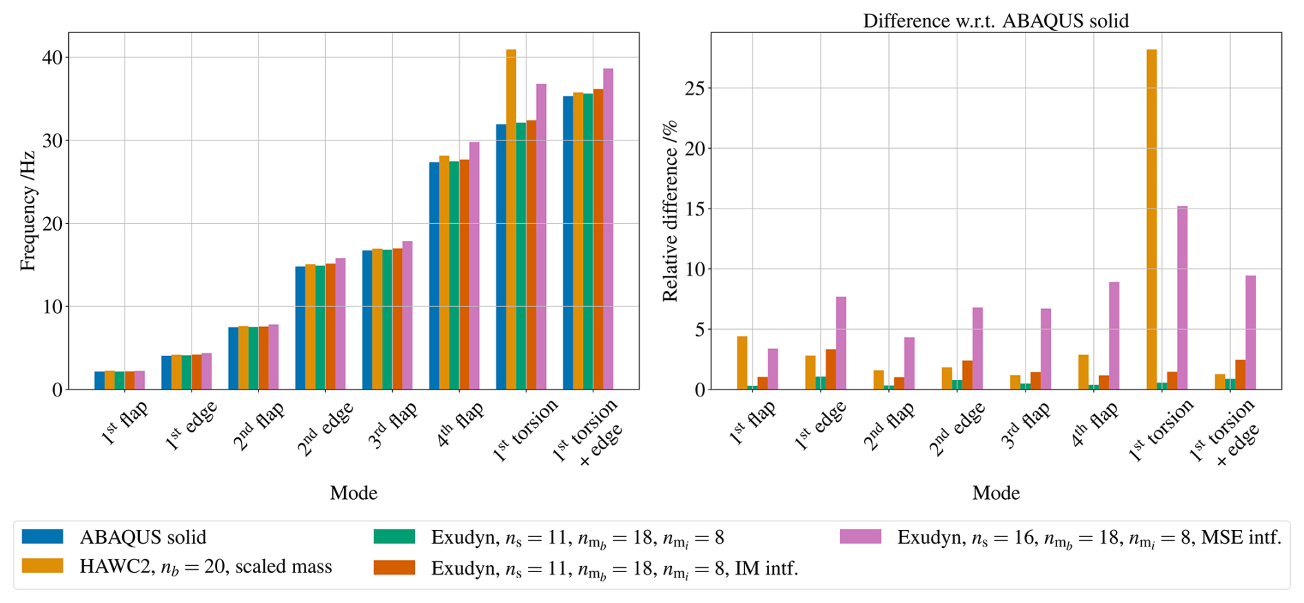
Figure 14 DTU 12.6 m blade: natural frequencies comparison. Relative differences calculated as $\left(f-f_{\mathrm{Abq}}\right)/f_{\mathrm{Abq}}$.

5 Conclusions

This paper presents a methodology to apply aerodynamic loads calculated with an aerodynamic BEM solver (typically found in wind turbine aeroelastic simulation tools) to a multibody FFRF-based reduced-order model built from solid finite elements and including interface reduction (with interface eigenmodes). It addresses two main challenges: not being able to directly apply the spanwise distributed aerodynamic loads computed from the BEM aerodynamic solver to such a model, given its inherently different nature from a one-dimensional beam model; and requiring one to apply loads at internal DOFs of the reduced-order model, which opposes the assumptions of the Hurty/Craig-Bampton method it is based on.

The proposed method consists of applying equivalent concentrated loads, calculated from the integration of the aerodynamic load distribution along multiple blade portions at the “centroid” of the spanwise load distribution. Interpolation multipoint constraints (RBE3) are used to apply the loads at each blade cross-section. These loads can be applied at any location of the reduced-order model by projecting them onto its subspace using the respective reduction basis. However, to avoid applying them at internal DOFs, two alternatives are presented, both based on adding interfaces at the load application locations: either using the same method employed for the existing substructuring interfaces (interface modes) or using the minimum strain energy formulation from Masarati et al. (2020), which is analogous to an RBE3 interface and therefore presents an option with a lower system size. The different versions of the multibody FFRF-based reduced-order model from solid elements (including or not internal load interfaces) are implemented in the multibody code Exudyn.

Two structures are analysed to assess the proposed methodology: a simple isotropic beam and an existing 12.6 m wind turbine blade manufactured at DTU. The nonlinear static response of the different models is compared with the reference solution from Abaqus and with HAWC2, as a baseline multibody FFRF-based model with beam elements. It is concluded from the analysis that applying equivalent concentrated loads is a reasonable approximation to distributed loads, although there will be an error resulting from not re-integrating the distributed load as the structure deforms; this error is expected to be more pronounced as larger deflections take place (an error of 7.5 % is observed for a transverse displacement corresponding to approximately 30 % of the beam length). With regard to the inclusion of internal load interfaces in the reduced-order models, it is found that it does not result in a significant gain in accuracy when compared to the baseline solution (without load interfaces). As observed in Sect. 4.1.2, the increase in accuracy is more evident for the torsional component, especially when the magnitude of the torsion moment is sufficiently large, but the error can also be mitigated by including torsion modes in the Hurty/Craig-Bampton reduction basis. Additionally, it is shown that the method including minimum strain energy load interfaces results in stiffer models and, consequently, less-accurate static responses: considering the DTU 12.6 m blade analysed, between 3 % and 15 % higher natural frequency values are computed w.r.t. the model without internal load interfaces.

The two multibody FFRF-based models considered in the analysis (HAWC2 and Exudyn) are in good agreement in the majority of cases, with the exception of the torsional behaviour of the DTU 12.6 m wind turbine blade. Both the twist response and torsional natural frequency computed by the HAWC2 beam model do not match the reference Abaqus solution, but those computed by the baseline Exudyn model do; namely, relative differences of approximately 28 % and 1 % are obtained for the torsional natural frequency with the HAWC2 and Exudyn models, respectively. This demonstrates the main advantage of the FFRF-based reduced-order models built from solid finite elements in being able to replicate the response of a high-fidelity FE model to a higher degree.

With this methodology, it becomes more feasible to integrate such a model within the framework of a multibody FFRF-based aeroelastic simulation tool such as HAWC2. The present work is, however, only a first step in this direction: important challenges remain, particularly regarding its application to dynamic (aeroelastic) simulations and the resulting computational efficiency of such an approach. Future work should therefore focus on analysing the dynamic response of this model, as well as its integration with a BEM-based aerodynamic solver. Another promising research direction is the coupling of this model with higher-fidelity aerodynamic models (e.g. 3D CFD, vortex lattice or panel methods) for applications beyond the one considered in this work.