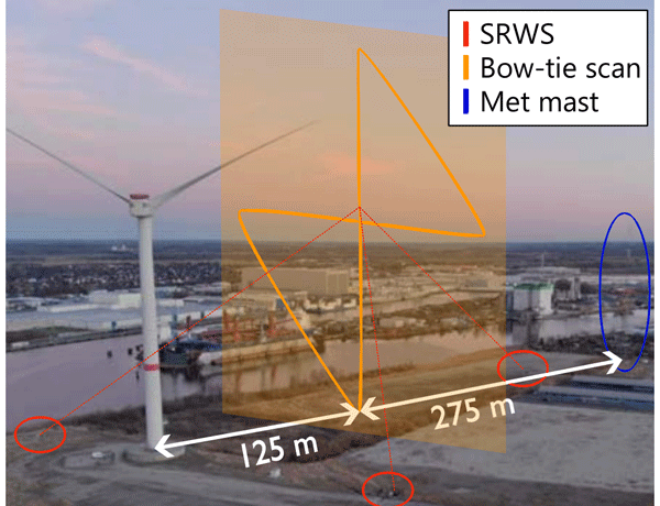
Turbulence characterization in near-coastal environment using triple short-range lidars and mast anemometry

Single- and two-point turbulence spectra derived from wind velocity measurements at a near-coastal site in northern Germany are analysed across a wide range of atmospheric-stability conditions. Spectral estimates are obtained from sonic and cup anemometer data, as well as from velocity time series reconstructed using a system of three synchronized short-range scanning lidars. A high level of agreement is observed at low and intermediate frequencies, with all measurement systems capturing key spectral features, including a plateau under convective conditions and a spectral gap in stable stratification. At higher frequencies, discrepancies arise due to spatial and temporal averaging effects inherent in the lidar and cup anemometer measurements. Spatial coherence estimates are comparatively less affected by these limitations and show high agreement, with exceptions. The synchronized lidar system is found to be highly suitable for coherence analysis, offering flexibility in terms of separation direction, distance, and height. Empirical models are fitted to the auto-spectra and coherence estimates to derive the model parameters as functions of atmospheric stability.

1 Introduction

Wind turbulence is characterized by single-point statistics, including velocity variances, spectra, and integral length scales, as well as two-point statistics describing spatial coherence. Both single- and two-point turbulence parameters have been identified as relevant drivers of ultimate and fatigue loads on bottom-fixed (Robertson et al., 2019) and floating (Wiley et al., 2023) wind turbines. In accordance with design standards such as the IEC 61400-1 by the International Electrotechnical Commission (IEC, 2005), synthetic wind fields are typically generated using either the uniform shear model (Mann, 1994) or the Kaimal spectrum (Kaimal et al., 1972) in combination with an exponential coherence model. These approaches are based on observations within the atmospheric surface layer, which generally extends up to approximately 100 m above ground. However, modern multi-megawatt windturbines exceed these heights and thus operate in regions where turbulence measurements are scarce.

The applicability of the IEC turbulence models is further restricted to neutral atmospheric conditions, in which turbulence is primarily governed by mechanical shear. Non-neutral stratification introduces buoyancy effects that influence both turbulence intensity and characteristic length scales. Højstrup (1982) addressed this by expressing velocity spectra observed in unstable boundary layers over smooth terrain in Minnesota as the sum of shear- and buoyancy-driven contributions. A similar formulation was proposed by Cheynet et al. (2018) based on sonic anemometer measurements over the North Sea. Both models have been applied to simulate the dynamic response of floating wind turbines, where the additional low-frequency energy under convective conditions was shown to increase several load components as well as platform rigid-body motions (Knight and Obhrai, 2019; Putri et al., 2020a).

Under stable conditions, negative buoyancy suppresses turbulent energy. Spectral modelling is further complicated by the presence of a spectral gap and large-scale, quasi-two-dimensional turbulent structures. These mesoscale fluctuations are typically neglected in aero-elastic simulations but become increasingly relevant for large floating wind turbines, with platform natural frequencies on the order of several minutes (Skaare et al., 2015; Allen et al., 2020). Syed and Mann (2024) proposed an extended version of the uniform shear model by incorporating a two-dimensional low-frequency component. The model was validated against offshore measurements and applied to simulate turbine response to synthetic wind fields with fluctuations up to periods of 1 h. The additional low-frequency energy was found to increase load components in the longitudinal direction, such as tower-base fore–aft and blade-root flapwise bending moments, as well as windward mooring line tension (Syed et al., 2026).

In addition to the influences of single-point turbulence spectra, wind turbine response is also affected by the spatial coherence of the inflow field. The horizontal asymmetry in wind speed across the rotor associated with reduced lateral coherence in the uniform shear model increases tower torsion, as demonstrated by Nybø et al. (2021) for a 10 MW bottom-fixed turbine. Similar trends have been reported for turbines on spar floaters (Doubrawa et al., 2019; Putri et al., 2020b) and semi-submersible platforms (Rivera-Arreba et al., 2022), which additionally exhibit increased platform yaw motions. Likewise, reduced vertical coherence leads to vertical load asymmetries across the rotor, resulting in increased tower-top fore–aft bending. In contrast, highly coherent wind fields imply that aerodynamic forces act largely in phase across the rotor. For bottom-fixed turbines, this increases tower-base fore–aft and flapwise blade bending moments (Nybø et al., 2021), while for floating turbines it has been associated with amplified surge and pitch motions and increased mooring line fatigue (Nybø et al., 2022; Rivera-Arreba et al., 2022).

Field measurements and numerical studies indicate that spectral coherence varies across wind components, separation distance and direction, measurement height, and atmospheric stability. However, comprehensive studies capturing all of these dependencies remain limited. Vertical coherence is commonly measured using meteorological masts (Cheynet et al., 2018; Midjiyawa et al., 2021), whereas lateral coherence has been investigated between multiple masts or along long-span bridges (Bowen et al., 1983; Hui et al., 2009).

In the absence of such structures, remote sensing with Doppler lidar systems provides an alternative. Single-lidar studies have examined coherence across lateral and vertical separations (Cheynet et al., 2016b; Lothon et al., 2006), as well as longitudinal separations (Davoust and von Terzi, 2016; Chen et al., 2021), although the estimates are limited to a single velocity component along the line of sight. Synchronized dual-lidar configurations enable coherence estimation of both along- and cross-wind turbulence, as demonstrated by Cheynet et al. (2016a) for a single 20 min record.

This approach was extended by Cheynet et al. (2021) and, more recently, Patel et al. (2026) using synchronized pulsed long-range lidars. The latter study investigates the lateral coherence of horizontal velocity components using instruments deployed at two sites along the west coast of Denmark. The results are remarkable, providing the first offshore coherence estimates across separations of 50 to 240 m and heights up to 270 m; however, they lack information on the vertical velocity component (Patel et al., 2026; Mann et al., 2026).

In this study, coherence is characterized at a near-coastal site using a triple-lidar system that enables reconstruction of the full three-component wind field (Giyanani et al., 2022; Meyer et al., 2024). The application of triple-lidar configurations for coherence estimation was first explored by Nafisifard et al. (2023), who reported lateral and vertical coherence over an 11 min period for separations of 10 and 20 m.

In the present work, nearly 500 h of lidar measurements acquired over a 5-month period are analysed to estimate three-dimensional wind coherence across lateral and vertical separations ranging from 10 to 160 m and at heights up to 230 m. The dataset was previously used by the authors to estimate coherence for a limited set of separations, revealing a strong dependence on both separation distance and measurement height (Vogt et al., 2026). The analysis was therefore extended to a broader range of separations located at various levels. In addition, the present work investigates single-point turbulence characteristics through auto-spectra and integral length scales. The lidar-based estimates are compared with measurements from a meteorological mast located 275 m away and equipped with sonic and cup anemometers.

The study pursues two main objectives. First, by comparing spectral estimates obtained from different sensor technologies, the respective strengths and limitations of the instruments for turbulence characterization are assessed. Second, the influence of atmospheric stability on turbulent wind spectra in a near-coastal environment is investigated to improve the design basis for wind turbine components. Empirical models for spectra and coherence are fitted to the observations to provide inputs for synthetic wind field generation in dynamic wind turbine response analysis.

In the following section, the test site and instrumentation are introduced. Section 3 describes the methodology, including data processing, atmospheric-stability classification, and the estimation and modelling of turbulence spectra. The results are presented and discussed in Sect. 4, focusing on atmospheric-stability distributions, turbulent length scales, auto-spectra, and vertical and lateral coherence. Finally, Sect. 5 summarizes the main findings and outlines directions for future work. The stability-dependent coefficients obtained by fitting empirical models to the turbulence spectra and coherence estimates are provided in Appendices A and B, respectively.

Figure 1 Elevation map of north-western Germany indicating the test site location. Created using the toolbox by Beauducel (2026) and data from ESA (2024).

Figure 2 Surface roughness length around the test site location. Created using the toolbox by Beauducel (2026) and data from ESA (2024).

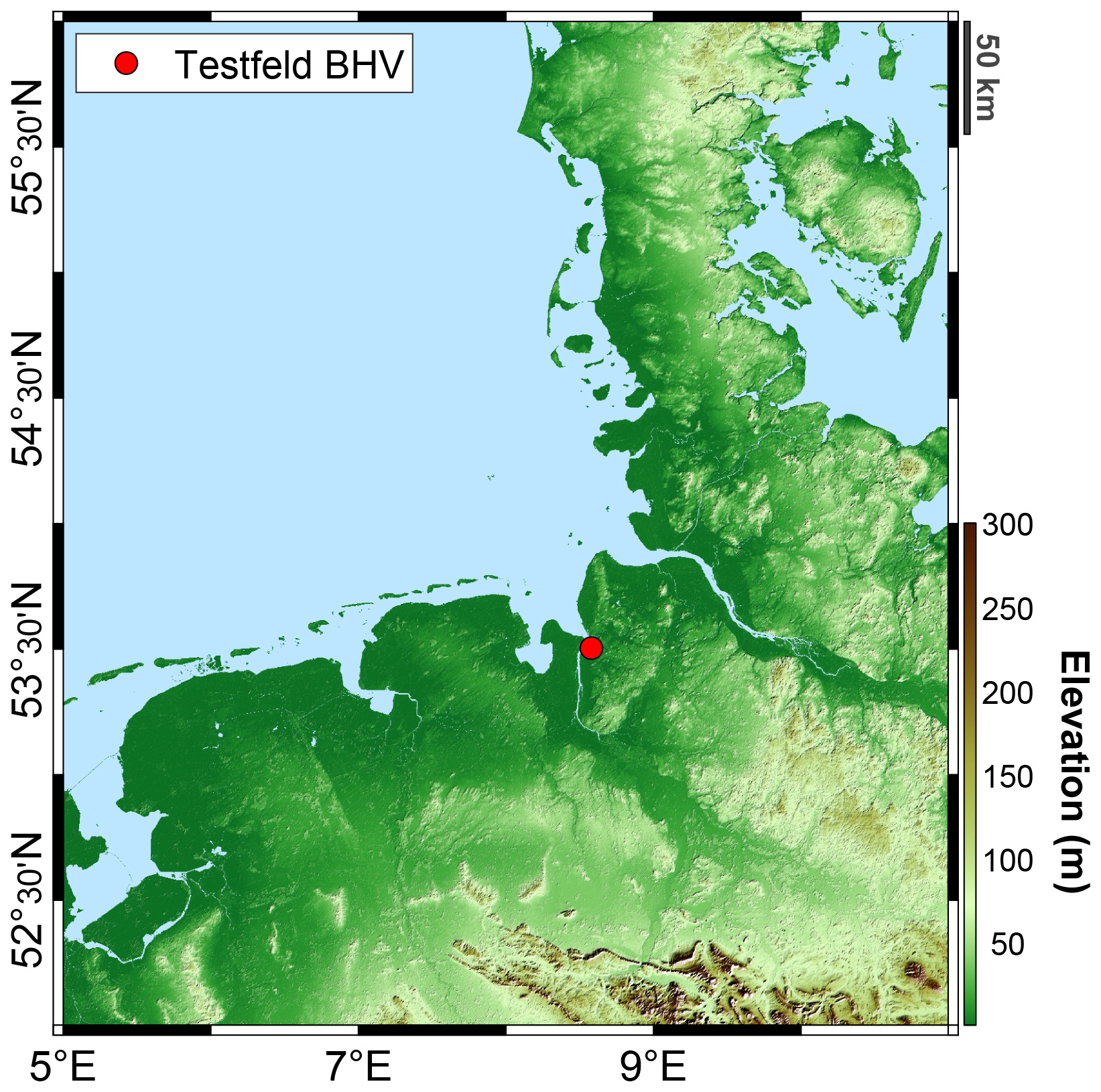
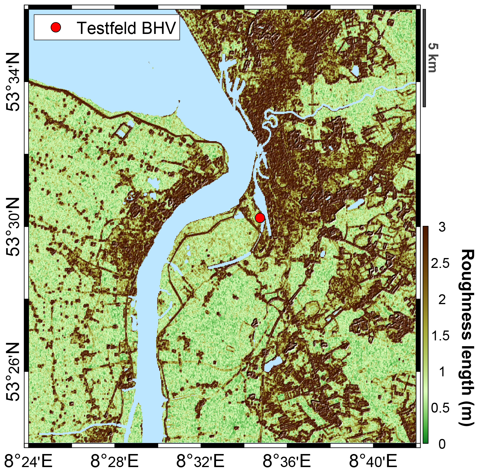
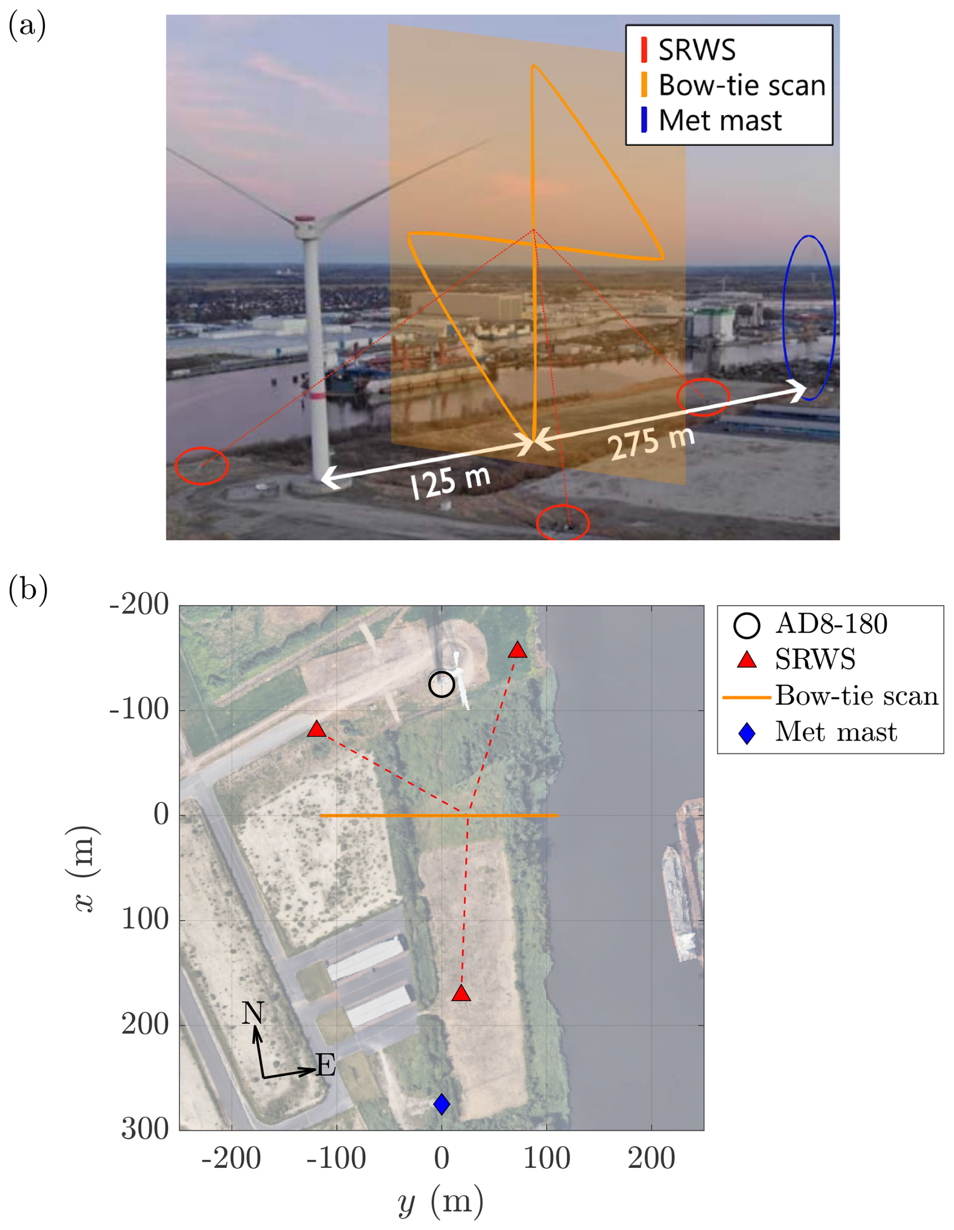
Figure 3 (a) Aerial view of the test site and (b) plan view showing the sensor locations in a fixed reference frame. Background imagery © Google, map data © 2009 GeoBasis-DE/BKG. Markers added by the authors.

2 Instrumentation

The datasets analysed in this work were collected during previous measurement campaigns at the Testfeld BHV located in Bremerhaven, Germany, on the east bank of the Weser estuary along the North Sea coast (53°30^′16^′′ N, 8°34^′43^′′ E). An elevation map of the region is shown in Fig. 1. The test site is situated on a former airfield near the town's fishing port. To the north through south-east in clockwise direction, there are several commercial buildings, with residential areas located further inland. The southern and south-western sectors are characterized by agricultural land and flat grassland. The Weser estuary lies north-west of the test site, resulting in a sector of approximately 30° where the flow reaches the site after traversing the sea surface. The roughness length of the surrounding area is illustrated in Fig. 2.

The test site comprises an Adwen AD8-180 prototype wind turbine and an IEC-compliant meteorological mast. For several months, three continuous-wave lidars based on the Short-Range WindScanner (SRWS) technology, developed by the DTU Department of Wind and Energy Systems (Mikkelsen et al., 2017b), were deployed around the turbine, as illustrated in Fig. 3. The SRWS system performed synchronized scans with the three lidars focusing on a common target within a vertical plane located 125 m from the turbine in the direction of the meteorological mast. Between October 2021 and April 2022, scans were conducted on 90 d following a so-called bow-tie pattern, consisting of a horizontal and a vertical line connected by two inclined segments. The centre of the bow tie was located at a height of z=125 m, corresponding to the turbine hub height.

The lidars recorded radial velocities along their respective lines of sight at a sampling rate of 322 Hz, while each bow-tie scan was completed in 2 s. The longitudinal, lateral, and vertical wind components are reconstructed from the individual line-of-sight velocities (Sect. 3.1) and mapped onto grid cells along the scanning trajectory. Time series are extracted at selected grid cells along the pattern, resulting in a temporal resolution of 1 Hz at the centre of the bow tie and 0.5 Hz at all other locations. The lidar probe lengths vary between 10 and 40 m, scaling quadratically with the distance between the instruments and the focus position along the bow-tie scan (Giyanani et al., 2022).

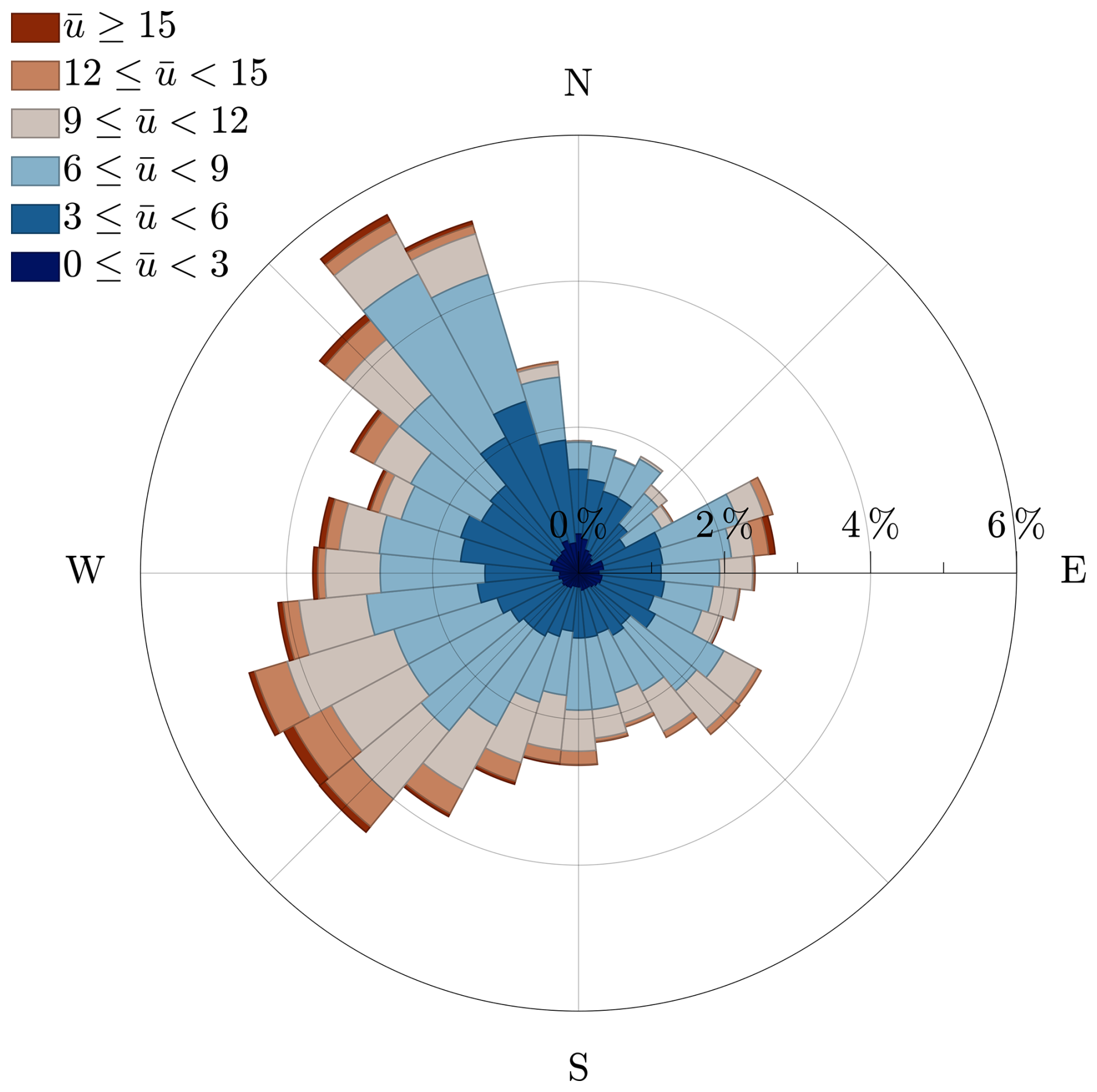
The meteorological mast is located 400 m south of the turbine, corresponding to a distance of 275 m from the SRWS scan plane. It is equipped with high-frequency sonic anemometers at $z_{\mathrm{sonic}}=\mathit{\{}\mathrm{25},\mathrm{55},\mathrm{110}\mathit{\}}\mathrm{m}$ and cup anemometers at $z_{\mathrm{cup}}=\mathit{\{}\mathrm{25},\mathrm{55},\mathrm{116}\mathit{\}}\mathrm{m}$. The sonic anemometers measure the three wind velocity components and temperature at 20 Hz, while the cup anemometers provide horizontal wind speed at 1 Hz. Mast data covering 533 d between January 2021 and August 2022 are analysed in this study. A wind rose for this period is shown in Fig. 4, indicating both the estuary (315 to 345°) and the grassland south-west of the test site (220 to 250°) as the prevailing wind directions.

Figure 4 Wind rose derived from sonic anemometer data at z=110 m. Visualized using the toolbox by Pereira (2026).

3 Methodology

3.1 Wind field reconstruction and data processing

The synchronized line-of-sight velocities v_r measured by the individual lidars are used to reconstruct the three-dimensional wind velocity field in a fixed reference frame (x and y as defined in Fig. 3b, z pointing vertically upward). The conversion was applied by Giyanani et al. (2022) and utilizes the instruments' scanning azimuth α and elevation angle β:

$$\begin{array}{}\text{(1)}& \left[\begin{array}{c}{v}_x\\ v_y\\ v_z\end{array}\right]={\left[\begin{array}{ccc}\cos {\mathit{\alpha }}_{\mathrm{1}}\cos {\mathit{\beta }}_{\mathrm{1}}& \sin {\mathit{\alpha }}_{\mathrm{1}}\cos {\mathit{\beta }}_{\mathrm{1}}& \sin {\mathit{\beta }}_{\mathrm{1}}\\ \cos {\mathit{\alpha }}_{\mathrm{2}}\cos {\mathit{\beta }}_{\mathrm{2}}& \sin {\mathit{\alpha }}_{\mathrm{2}}\cos {\mathit{\beta }}_{\mathrm{2}}& \sin {\mathit{\beta }}_{\mathrm{2}}\\ \cos {\mathit{\alpha }}_{\mathrm{3}}\cos {\mathit{\beta }}_{\mathrm{3}}& \sin {\mathit{\alpha }}_{\mathrm{3}}\cos {\mathit{\beta }}_{\mathrm{3}}& \sin {\mathit{\beta }}_{\mathrm{3}}\end{array}\right]}^{-\mathrm{1}}\left[\begin{array}{c}{v}_{\text{r,}\mathrm{1}}\\ v_{\text{r,}\mathrm{2}}\\ v_{\text{r,}\mathrm{3}}\end{array}\right].\end{array}$$

Here, the azimuth angle is defined with respect to the x axis in Fig. 3b. The velocity components v_x, v_y, and v_z are also available from the sonic anemometers. In contrast, the cup anemometers provide only the horizontal wind speed v_hor, defined as

$$\begin{array}{}\text{(2)}& v_{\mathrm{hor}}={\left(v_x^{\mathrm{2}}+v_y^{\mathrm{2}}\right)}^{\mathrm{1}/\mathrm{2}}.\end{array}$$

All time series are post-processed using range filters of $\pm \mathrm{30}\mathrm{m}{\mathrm{s}}^{-\mathrm{1}}$ for the horizontal velocity components and $\pm \mathrm{5}\mathrm{m}{\mathrm{s}}^{-\mathrm{1}}$ for the vertical component, together with a maximum step size of $\pm \mathrm{3}\mathrm{m}{\mathrm{s}}^{-\mathrm{1}}$. Additional despiking is achieved using a rolling median filter with a window length of 0.5 s for the high-frequency sonic measurements and seven samples for the cup anemometer and SRWS time series. Further instrument-specific filters were previously applied to the sonic velocity and temperature measurements by Meyer (2024).

The time series are segmented into samples with an averaging period of 30 min. For each sample, the mean horizontal ($\stackrel{\mathrm{‾}}{\mathit{\varphi }}$) and vertical ($\stackrel{\mathrm{‾}}{\mathit{\psi }}$) wind directions are calculated as

$$\begin{array}{}\text{(3)}& \stackrel{\mathrm{‾}}{\mathit{\varphi }}=\text{atan}(\stackrel{\mathrm{‾}}{v_y},\stackrel{\mathrm{‾}}{v_x})\end{array}$$

and

$$\begin{array}{}\text{(4)}& \stackrel{\mathrm{‾}}{\mathit{\psi }}=\text{atan}(\stackrel{\mathrm{‾}}{v_z},\stackrel{\mathrm{‾}}{v_{\mathrm{hor}}}).\end{array}$$

The longitudinal, lateral, and vertical velocity components in the mean wind coordinate system are obtained through double rotation:

$$\begin{array}{}\text{(5)}& \left[\begin{array}{c}u\\ v\\ w\end{array}\right]=\left[\begin{array}{ccc}\cos \stackrel{\mathrm{‾}}{\mathit{\varphi }}\cos \stackrel{\mathrm{‾}}{\mathit{\psi }}& \sin \stackrel{\mathrm{‾}}{\mathit{\varphi }}\cos \stackrel{\mathrm{‾}}{\mathit{\psi }}& \sin \stackrel{\mathrm{‾}}{\mathit{\psi }}\\ -\sin \stackrel{\mathrm{‾}}{\mathit{\varphi }}& \cos \stackrel{\mathrm{‾}}{\mathit{\varphi }}& \mathrm{0}\\ -\cos \stackrel{\mathrm{‾}}{\mathit{\varphi }}\sin \stackrel{\mathrm{‾}}{\mathit{\psi }}& -\sin \stackrel{\mathrm{‾}}{\mathit{\varphi }}\sin \stackrel{\mathrm{‾}}{\mathit{\psi }}& \cos \stackrel{\mathrm{‾}}{\mathit{\psi }}\end{array}\right]\left[\begin{array}{c}{v}_x\\ v_y\\ v_z\end{array}\right].\end{array}$$

The fluctuating velocity components u^′, v^′, and w^′ are subsequently obtained by linear detrending within each sample. Only samples with a data availability above 90 % and a mean wind speed $\overline{u}$ between 3 and 28 m s⁻¹ are retained. Samples exhibiting atypical fluctuations are removed by excluding cases with turbulence intensities of I_u>0.20, I_v>0.18, or I_w>0.15, as well as those with I<0.01. First- and second-order stationarity in wind speed and direction are ensured by constraining the allowable relative error between moving and static estimates of the mean and standard deviation. Wake conditions are excluded by filtering out samples with a turbine in operation and mean wind directions of $\stackrel{\mathrm{‾}}{\mathit{\varphi }}=\mathrm{349}$ to 29° for the mast sensors and $\stackrel{\mathrm{‾}}{\mathit{\varphi }}=\mathrm{309}$ to 69° for the SRWS measurements. Additional 45° sectors are removed from the sonic and cup anemometer data to avoid mast-induced flow distortion. Finally, the datasets are filtered to include only atmospheric-stability conditions satisfying $\left|\mathit{\zeta }\right|\le \mathrm{2}$. The estimation of the non-dimensional stability parameter ζ is described in Sect. 3.2.

Table 1 Number of available 30 min samples for the different sensors throughout the filtering process.

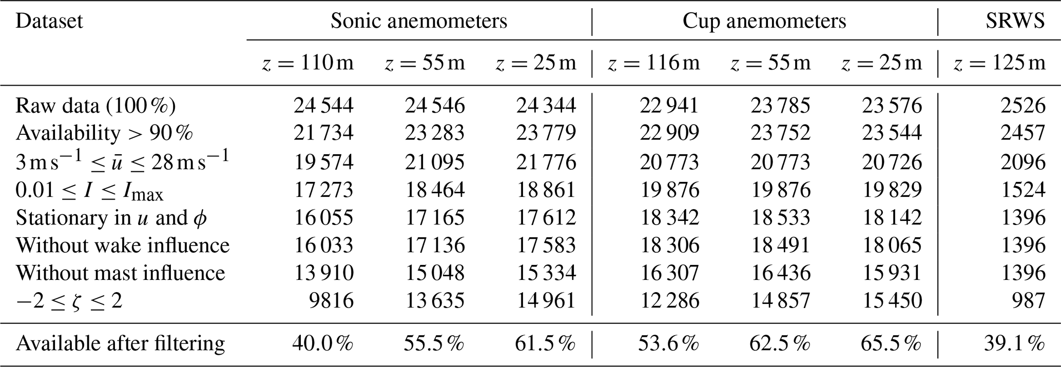
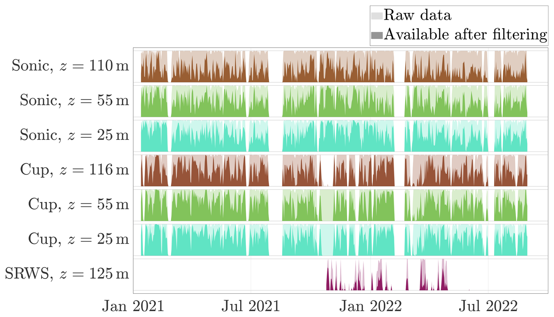
Figure 5 Number of available 30 min samples per day for the different sensors before and after filtering. In each subplot, the vertical axis range spans from 0 to 48 samples, the latter corresponding to an availability of 100 %.

The number of samples N remaining after each filtering step is summarized in Table 1 for the individual sensors. Figure 5 further illustrates the data availability before and after filtering over the 20-month study period. Prior to applying the atmospheric-stability filter, approximately 57 % to 63 % of the sonic anemometer data remain available. Restricting the dataset to $\left|\mathit{\zeta }\right|\le \mathrm{2}$ reduces the availability to 40.0 %, 55.5 %, and 61.5 % for the upper, intermediate, and lower measurement levels, respectively. The reduced availability at higher elevations is primarily due to the more frequent occurrence of stability conditions outside the selected range. Closer to the surface, enhanced mechanically generated turbulence contributes to the higher occurrence of near-neutral conditions, resulting in a larger fraction of data satisfying the stability criterion. For the cup anemometers, the availability is slightly higher (53.6 % to 65.5 %), as fewer values are removed by outlier detection, and fewer cases exhibit turbulence intensities exceeding 20 %. The high-frequency filtering behaviour of the cup anemometers is further discussed in Sect. 4.2.2.

For the SRWS measurements, the final data availability is the lowest (39.1 %), despite the absence of an azimuth filter for mast-induced flow distortion. This primarily results from the turbulence intensity filter, which removes approximately 27 % of SRWS samples, compared to about 4 % for the cup anemometers and 12 % for the sonics. The SRWS time series were found to contain larger portions of unrealistic fluctuations and outliers. Even after filtering, a residual influence is visible in the auto-spectra, as discussed in Sect. 4.2.2. Although Table 1 indicates that no SRWS samples were explicitly removed to avoid wake conditions, 50 potential wake cases were identified. However, 32 of these were previously excluded due to excessive turbulence intensity, while the remaining 18 samples were classified as non-stationary.

3.2 Atmospheric-stability classification

The velocity spectra are classified using the non-dimensional stability parameter ζ. It is defined as the ratio of the measurement height z to the local Obukhov length L, which represents the height at which buoyant and shear-driven turbulence generation are at balance.

$$\begin{array}{}\text{(6)}& \mathit{\zeta }={\displaystyle \frac{z}{L}}={\displaystyle \frac{-g\mathit{\kappa }z\stackrel{\mathrm{‾}}{w^{\prime }{\mathit{\theta }}_{\mathrm{v}}^{\prime }}}{\stackrel{\mathrm{‾}}{{\mathit{\theta }}_{\mathrm{v}}}{u}_{*}^{\mathrm{3}}}}.\end{array}$$

Here, g denotes the gravitational acceleration, κ≈0.4 the von Kármán constant, and u_* the friction velocity, which is estimated as

$$\begin{array}{}\text{(7)}& u_{*}={\left({\stackrel{\mathrm{‾}}{u^{\prime }{w}^{\prime }}}^{\mathrm{2}}+{\stackrel{\mathrm{‾}}{v^{\prime }{w}^{\prime }}}^{\mathrm{2}}\right)}^{\mathrm{1}/\mathrm{4}}.\end{array}$$

The virtual potential temperature θ_v is approximated using the absolute sonic temperature observations, following Schotanus et al. (1983) and Cheynet et al. (2018). Samples are grouped into 15 stability classes using the bin edges $\left|\mathit{\zeta }\right|=\mathit{\{}\mathrm{0.1},\mathrm{0.2},\mathrm{0.4},\mathrm{0.6},\mathrm{0.9},\mathrm{1.2},\mathrm{1.6},\mathrm{2.0}\mathit{\}}$, where $\mathit{\zeta }<-\mathrm{0.1}$ represents unstable, $\left|\mathit{\zeta }\right|\le \mathrm{0.1}$ neutral, and ζ>0.1 stable conditions. The stability parameter ζ is calculated locally for each sonic anemometer and used to classify the auto-spectra derived from the sonic and cup anemometers at the corresponding heights. To classify spectral coherence measured along the mast, the mean value of ζ between the respective sonics is used. Samples for which the two individual stability estimates differ by more than three classes are discarded to increase the reliability of the classification. The SRWS spectra and coherence estimates are classified using ζ derived from the sonic at z=110 m, as it is the closest available reference to most locations along the bow-tie scan. The observed distributions of atmospheric stability across mean wind speed, direction, month, and time of day are discussed in Sect. 4.1.

Table 2 Available wind components, Nyquist frequency, and measurement heights for the estimation of auto-spectra from each instrument.

Table 3 Available wind components as well as vertical and lateral separation distances for the estimation of spectral coherence from each instrument.

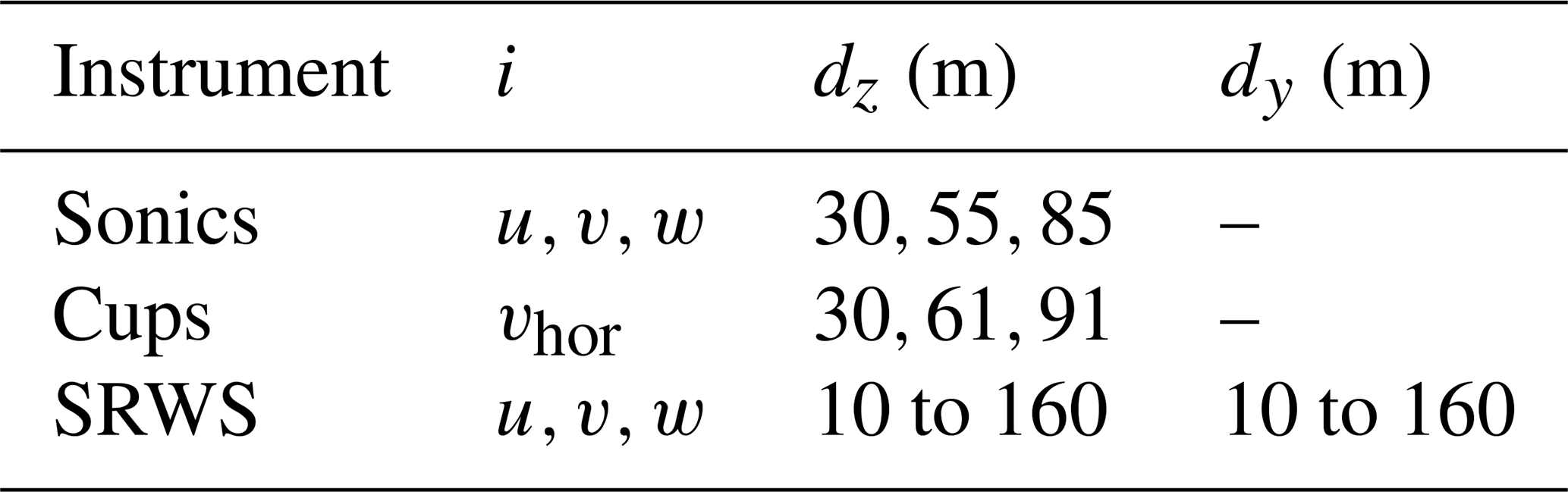
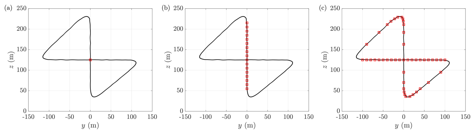
Figure 6 Bow-tie scan pattern showing grid cells used to extract velocity time series for calculation of (a) auto-spectra, (b) vertical coherence, and (c) lateral coherence.

3.3 Estimation of single- and two-point velocity spectra

Auto-spectra are computed using Welch's method (Welch, 1967) with a single Hamming window, enabling the analysis of the low-frequency regime down to 0.556 mHz. The large number of available samples ensures sufficient ensemble averaging to produce smooth spectral estimates. Coherence estimates, which are typically noisier, are obtained with additional averaging resulting from the use of three segments with 50 % overlap.

For the mast sensors, auto-spectra are calculated at each installation height listed in Table 2. The Nyquist frequency f_N is 10 Hz for the sonics and 0.5 Hz for the cup anemometers. To obtain f_N=0.5 Hz also for the lidar-based spectra, velocity time series are extracted from a grid cell at the bow-tie centre (z=125 m), which is intersected twice per scan cycle.

Vertical coherence is assessed along the meteorological mast between the individual cup and sonic anemometers. Three vertical separations d_z are available, spanning from 30 m between the lower sensors to approximately 60 m between the upper pair and about 90 m between the lowest and highest measurement levels. The precise values of the separation distances are listed in Table 3.

The SRWS system provides more flexibility; time series are extracted along the vertical line of the bow tie at heights between 55 and 215 m, resulting in separations ranging from 10 to 160 m (Fig. 6b). Lateral coherence is obtained similarly along the horizontal line of the bow tie. Further lateral coherence estimates are computed between the vertical line and the inclined segments (Fig. 6c), enabling an assessment of height effects on lateral coherence.

The coherence of a velocity component $i=\mathit{\{}u,v,w\mathit{\}}$ between two points in space is defined as the cross-spectrum S_i,12(f) normalized by the geometric mean of the auto-spectra S_i,1(f) and S_i,2(f). In this study, unless stated otherwise, coherence refers specifically to the co-coherence γ_ij, i.e. the real part of the complex coherence:

$$\begin{array}{}\text{(8)}& {\mathit{\gamma }}_{ij}\left(f\right)=\text{Re}\left[{\displaystyle \frac{S_{i,\mathrm{12}}\left(f\right)}{\sqrt{S_{i,\mathrm{1}}\left(f\right)S_{i,\mathrm{2}}\left(f\right)}}}\right],\end{array}$$

with f denoting the frequency in hertz and $j=\mathit{\{}x,y,z\mathit{\}}$ the separation direction.

When estimating coherence between two SRWS grid cells along the scanning trajectory, a time lag τ_scan arises, ranging from 0.026 s for 10 m separations to 0.52 s for the furthest separated grid cells. The cross-spectrum of two shifted time series is corrected as

$$\begin{array}{}\text{(9)}& S_{i,\mathrm{12}}^{\mathrm{corr}.}\left(f\right)=S_{i,\mathrm{12}}\left(f\right)\left[\cos \left(\mathrm{2}\mathit{\pi }f\mathit{\tau }\right)+i\sin \left(\mathrm{2}\mathit{\pi }f\mathit{\tau }\right)\right].\end{array}$$

For lateral coherence, horizontal wind directions non-normal to the bow-tie plane introduce an additional time shift τ_ε due to the longitudinal separation d_x resulting from the wind-direction offset ε. The total time lag τ used for the phase correction is therefore given by the sum of the scanning-induced delay τ_scan and the longitudinal delay τ_ε, which is estimated as

$$\begin{array}{}\text{(10)}& {\mathit{\tau }}_{\mathit{\epsilon }}={\displaystyle \frac{d_x}{\overline{u}}}={\displaystyle \frac{d_y\sin \mathit{\epsilon }}{\overline{u}}}.\end{array}$$

This approximation is based on the assumption of frozen turbulence. To limit the associated uncertainties, lateral coherence estimates are filtered for horizontal wind directions producing a maximum offset of $\mathit{\epsilon }=\pm \mathrm{15}$°.

In this study, coherence estimates are expressed as functions of the wavenumber k, normalized by the separation distance d_j,

$$\begin{array}{}\text{(11)}& k{d}_j={\displaystyle \frac{\mathrm{2}\mathit{\pi }f{d}_j}{\overline{u}}},\end{array}$$

while auto-spectra are presented over the reduced frequency n:

$$\begin{array}{}\text{(12)}& n={\displaystyle \frac{fz}{\overline{u}}}.\end{array}$$

3.4 Turbulence modelling

In line with the IEC 61400-1 standard for wind turbine design requirements (IEC, 2005), turbulent velocity spectra in wind energy applications are commonly represented using either the uniform shear model (Mann, 1994) or the Kaimal spectrum (Kaimal et al., 1972). The latter is defined as

$$\begin{array}{}\text{(13)}& {\displaystyle \frac{f{S}_i\left(n\right)}{{\mathit{\sigma }}_i^{\mathrm{2}}}}={\displaystyle \frac{\mathrm{4}n{L}_i{z}^{-\mathrm{1}}}{{\left(\mathrm{1}+\mathrm{6}n{L}_i{z}^{-\mathrm{1}}\right)}^{\mathrm{5}/\mathrm{3}}}},\end{array}$$

where σ_i denotes the standard deviation of the velocity component, and L_i is the corresponding integral length scale,

$$\begin{array}{}\text{(14)}& L_i=\left\{\begin{array}{rlrl}{\displaystyle }& {\displaystyle }\mathrm{8.1}{\mathrm{\Lambda }}_{\mathrm{1}}& {\displaystyle }& {\displaystyle }\text{for}i=u\\ {\displaystyle }& {\displaystyle }\mathrm{2.7}{\mathrm{\Lambda }}_{\mathrm{1}}& {\displaystyle }& {\displaystyle }\text{for}i=v\\ {\displaystyle }& {\displaystyle }\mathrm{0.66}{\mathrm{\Lambda }}_{\mathrm{1}}& {\displaystyle }& {\displaystyle }\text{for}i=w\end{array}\right.,\end{array}$$

which is a function of the scale parameter Λ₁:

$$\begin{array}{}\text{(15)}& {\mathrm{\Lambda }}_{\mathrm{1}}=\left\{\begin{array}{rlrl}{\displaystyle }& {\displaystyle }\mathrm{0.7}z& {\displaystyle }& {\displaystyle }\text{if}z\le \mathrm{60}\mathrm{m}\\ {\displaystyle }& {\displaystyle }\mathrm{42}\text{m}& {\displaystyle }& {\displaystyle }\text{if}z\ge \mathrm{60}\mathrm{m}\end{array}\right..\end{array}$$

Under the assumption of frozen turbulence, the streamwise integral length scale can be estimated from a single-point velocity time series as

$$\begin{array}{}\text{(16)}& L_i=\overline{u}{T}_i,\end{array}$$

where T_i is an integral timescale obtained by fitting an exponential decay function to the auto-correlation function R_i(τ) of the velocity signal:

$$\begin{array}{}\text{(17)}& R_i\left(\mathit{\tau }\right)=\text{exp}\left(-{\displaystyle \frac{\mathit{\tau }}{T_i}}\right).\end{array}$$

Throughout this work, L_i denotes the streamwise integral length scale of velocity component i.

The Kaimal spectrum can be approximated by a bilinear representation consisting of an energy-containing range with constant spectral density and an inertial subrange characterized by $S_i\left(n\right)\propto f^{-\mathrm{5}/\mathrm{3}}$. Several experimental studies (Drobinski et al., 2004; Mikkelsen et al., 2017a; Cheynet et al., 2018) have identified an intermediate transition range within the atmospheric surface layer, where $S_i\left(n\right)\propto f^{-\mathrm{1}}$. When pre-multiplied by frequency, the transition range forms a spectral plateau, bounded by regions exhibiting +1 and $-\mathrm{2}/\mathrm{3}$ power-law behaviour. Cheynet et al. (2018) proposed an extended formulation of the Kaimal spectrum to capture this shape, referred to as the pointed–blunt model,

$$\begin{array}{}\text{(18)}& {\displaystyle \frac{f{S}_i\left(n\right)}{{\mathit{\sigma }}_i^{\mathrm{2}}}}={\displaystyle \frac{a_{\mathrm{1}}^{i}n}{{\left(\mathrm{1}+b_{\mathrm{1}}^{i}n\right)}^{\mathrm{5}/\mathrm{3}}}}+{\displaystyle \frac{a_{\mathrm{2}}^{i}n}{\mathrm{1}+b_{\mathrm{2}}^i{n}^{\mathrm{5}/\mathrm{3}}}},\end{array}$$

where $a_{\mathrm{1}}^i$, $a_{\mathrm{2}}^i$, $b_{\mathrm{1}}^i$, and $b_{\mathrm{2}}^i$ are empirical parameters that vary with wind component, measurement height, and atmospheric stability. Figure 7 illustrates the spectral shapes of the Kaimal spectrum, the pointed–blunt model, and their corresponding piecewise power-law approximations.

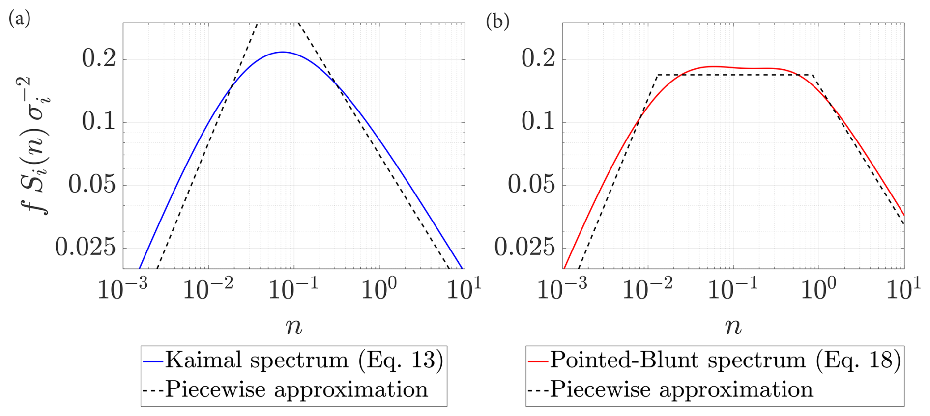
Figure 7 Spectral representations of (a) the Kaimal model and (b) the pointed–blunt model, including piecewise power-law approximations with exponents +1, 0, and $-\mathrm{2}/\mathrm{3}$.

In Sect. 4.2.2, Eq. (18) is fitted to the measured spectra under unstable to neutral atmospheric conditions. For stable conditions, an additional low-frequency contribution is observed, particularly for the horizontal velocity components, likely associated with mesoscale motions. As demonstrated in several theoretical and experimental studies (Kraichnan, 1967; Nastrom et al., 1984; Larsén et al., 2016), the spectral density in the mesoscale range follows a $S_i\left(n\right)\propto f^{-\mathrm{5}/\mathrm{3}}$ scaling. At the same time, microscale turbulence no longer displays a well-defined plateau but instead exhibits a distinct spectral peak. In this work, the stable velocity spectra are thus described by

$$\begin{array}{}\text{(19)}& {\displaystyle \frac{f{S}_i\left(n\right)}{{\mathit{\sigma }}_i^{\mathrm{2}}}}={\displaystyle \frac{a_{\mathrm{2}}^{i}n}{\mathrm{1}+b_{\mathrm{2}}^i{n}^{\mathrm{5}/\mathrm{3}}}}+a_{\mathrm{3}}^i{n}^{-\mathrm{2}/\mathrm{3}}.\end{array}$$

The first term in Eq. (19), referred to as the pointed model, represents the microscale turbulence peak, whereas the second term accounts for the mesoscale contribution.

3.5 Coherence modelling

Coherence models are employed to introduce spatial correlation into synthetic wind fields generated using stochastic turbulence models. The IEC 61400-1 standard (IEC, 2005) proposes the following expression in combination with the Kaimal spectrum:

$$\begin{array}{}\text{(20)}& {\mathit{\gamma }}_{uj}\left(k{d}_j\right)=\text{exp}\left\{-\mathrm{12}{\left[{\left({\displaystyle \frac{k{d}_j}{\mathrm{2}\mathit{\pi }}}\right)}^{\mathrm{2}}+{\left({\displaystyle \frac{\mathrm{0.12}{d}_j}{L_u}}\right)}^{\mathrm{2}}\right]}^{\mathrm{0.5}}\right\},\end{array}$$

which is limited to the longitudinal velocity component. A more general formulation was introduced by Davenport (1961):

$$\begin{array}{}\text{(21)}& {\mathit{\gamma }}_{ij}\left(k{d}_j\right)=\text{exp}\left({\displaystyle \frac{-C_{ij}k{d}_j}{\mathrm{2}\mathit{\pi }}}\right),\end{array}$$

where C_ij is an empirical decay coefficient associated with velocity component $i=\mathit{\{}u,v,w\mathit{\}}$ and separation direction $j=\mathit{\{}x,y,z\mathit{\}}$. This formulation implies γ_ij(0)=1, which is only valid when the separation distance is small compared to the dominant turbulence length scales. For the vertical velocity component, this assumption is often violated, and even for the horizontal components, deviations from unity coherence at k=0 may occur for large separations or at low heights with pronounced surface effects.

To account for this, a scaling coefficient $A_{ij}\in [\mathrm{0},\mathrm{1}]$ is introduced in this work:

$$\begin{array}{}\text{(22)}& {\mathit{\gamma }}_{ij}\left(k{d}_j\right)=A_{ij}\text{exp}\left({\displaystyle \frac{-C_{ij}k{d}_j}{\mathrm{2}\mathit{\pi }}}\right).\end{array}$$

To account for the dependence of coherence on the separation distance and the measurement height, both the scaling and the decay coefficient are expressed as exponential functions of the ratio $d_j{\overline{z}}^{-\mathrm{1}}$:

$$\begin{array}{}\text{(23)}& {\displaystyle }{C}_{ij}\left({\displaystyle \frac{d_j}{\overline{z}}}\right)=c_{\mathrm{1}}^{ij}\text{exp}\left(c_{\mathrm{2}}^{ij}{\displaystyle \frac{d_j}{\overline{z}}}\right),\text{(24)}& {\displaystyle }{A}_{ij}\left({\displaystyle \frac{d_j}{\overline{z}}}\right)=\text{exp}\left(-c_{\mathrm{3}}^{ij}{\displaystyle \frac{d_j}{\overline{z}}}\right),\end{array}$$

where $\overline{z}$ denotes the average height of the two points. Substituting Eqs. (23) and (24) into Eq. (22) yields a three-parameter coherence model:

$$\begin{array}{}\text{(25)}& {\mathit{\gamma }}_{ij}\left(k{d}_j\right)=\text{exp}\left[-{\displaystyle \frac{k{d}_j}{\mathrm{2}\mathit{\pi }}}{c}_{\mathrm{1}}^{ij}\text{exp}\left(c_{\mathrm{2}}^{ij}{\displaystyle \frac{d_j}{\overline{z}}}\right)-c_{\mathrm{3}}^{ij}{\displaystyle \frac{d_j}{\overline{z}}}\right].\end{array}$$

For small separations or large heights, this formulation reduces to the Davenport model. For other conditions, Eq. (25) allows for γ_ij(0)<1. Moreover, by incorporating the normalized separation distance $d_j{\overline{z}}^{-\mathrm{1}}$, the coefficients c₁, c₂, and c₃ become functions of atmospheric stability only. In contrast, the original Davenport coefficient is typically observed to also depend on separation distance and measurement height (Bowen et al., 1983; Cheynet et al., 2018).

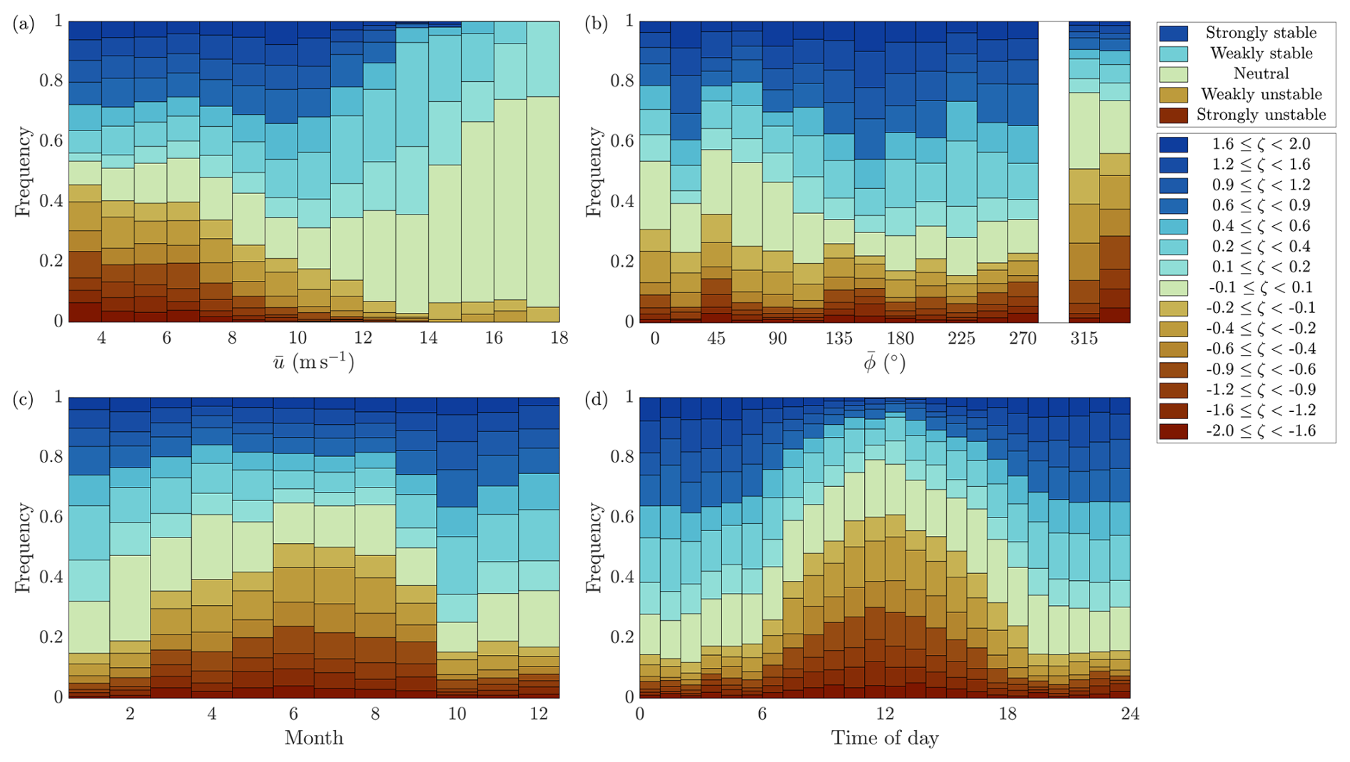
Figure 8 Occurrence of atmospheric-stability classes as a function of (a) mean wind speed, (b) mean wind direction, (c) month, and (d) time of day, based on sonic anemometer measurements at z=110 m. Data within 270 to 315° are excluded to avoid mast-induced flow distortion.

4 Results and discussion

4.1 Atmospheric-stability distributions

Figure 8 presents the occurrence of the different stability classes within bins of mean wind speed and direction, as well as their variation over the course of the year and the diurnal cycle. Here, the non-dimensional stability parameter ζ is derived from the sonic anemometer measurements at z=110 m. The corresponding distributions at z=55 m and z=25 m are provided in Appendix C.

At low wind speeds, stable and unstable conditions occur with comparable frequency, whereas neutral conditions account for less than 10 %. With increasing wind speed, mechanically generated turbulence becomes more dominant, and buoyancy effects diminish. As a result, the occurrence of unstable conditions decreases nearly linearly and remains below 8 % for $\overline{u}>\mathrm{12}\mathrm{m}{\mathrm{s}}^{-\mathrm{1}}$. In contrast, stable conditions initially increase in frequency, reaching a maximum of approximately 70 % at $\overline{u}=\mathrm{10}$ to 11 m s⁻¹ before declining at higher wind speeds. Comparable trends were reported by Cheynet et al. (2018) at 41.5 m height at the FINO1 research platform in the North Sea, although with a noticeably lower proportion of stable conditions.

The distribution across wind direction is more uniform. Unstable conditions account for roughly 20 % overall but increase to about 50 % within the north-western sector with flow from over the estuary. Stable conditions are least frequent in this sector and become more prevalent for southern, inland directions. Data within 270 to 315° have been excluded to avoid mast-induced flow distortion.

The annual distribution exhibits a peak of unstable conditions during June and July, reflecting elevated soil surface temperatures. A pronounced diurnal cycle is observed as well, with unstable conditions reaching approximately 50 % around midday and stable atmospheres dominating during night-time hours with frequencies up to 75 %. Both the seasonal and diurnal patterns are characteristic of onshore environments, supporting the reliability of the stability classification.

4.2 Single-point turbulence characteristics

4.2.1 Integral length scales

Figure 9 presents the integral length scales of the velocity components as a function of height. The IEC 61400-1 values (Eq. 14) are compared with estimates obtained from a least-square fit of the Kaimal spectrum (Eq. 13) to measured spectra under neutral conditions, as well as from an exponential fit to the auto-correlation function according to Eqs. (16)–(17).

At heights z<60 m, the length scales estimated using both methods generally fall below the IEC reference values. The only exception is the vertical length scale obtained from the fitted Kaimal spectrum, which slightly exceeds the standard value. At z>100 m, the Kaimal-based estimates are consistently larger than the IEC reference. In contrast, the length scales derived from the auto-correlation functions tend to underestimate the horizontal components while providing closer agreement for L_w.

The IEC 61400-1 standard proposes linearly increasing length scales up to a level of 60 m, remaining constant above this height. The estimates obtained from the auto-correlation functions mostly support this trend, showing only minor increases in L_i from 55 to 125 m. The length scales derived by fitting the Kaimal spectrum, however, appear to increase linearly up to a height of 110 m and even stronger at the highest level, which is based on SRWS measurements. A similar overestimation of lidar-based length scales was reported by Cheynet et al. (2016a) for the horizontal velocity components obtained from dual-lidar measurements and partially attributed to spatial averaging effects.

Figure 9 Integral length scales under neutral conditions according to IEC 61400-1 (IEC, 2005), compared with estimates obtained from a least-square fit of the Kaimal spectrum and from the auto-correlation function.

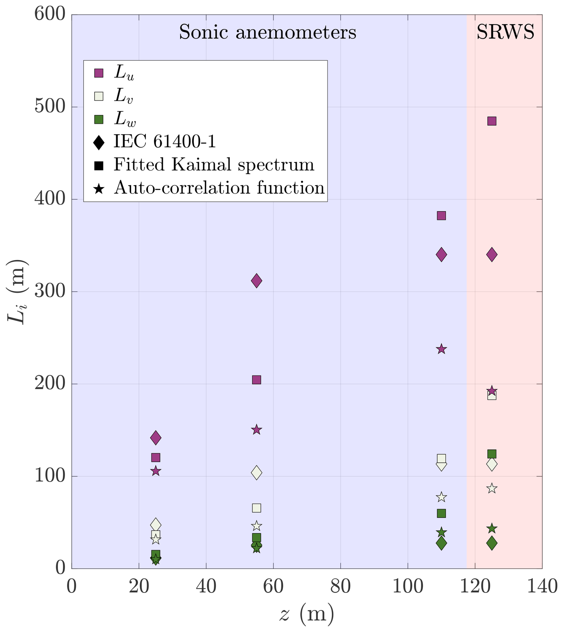
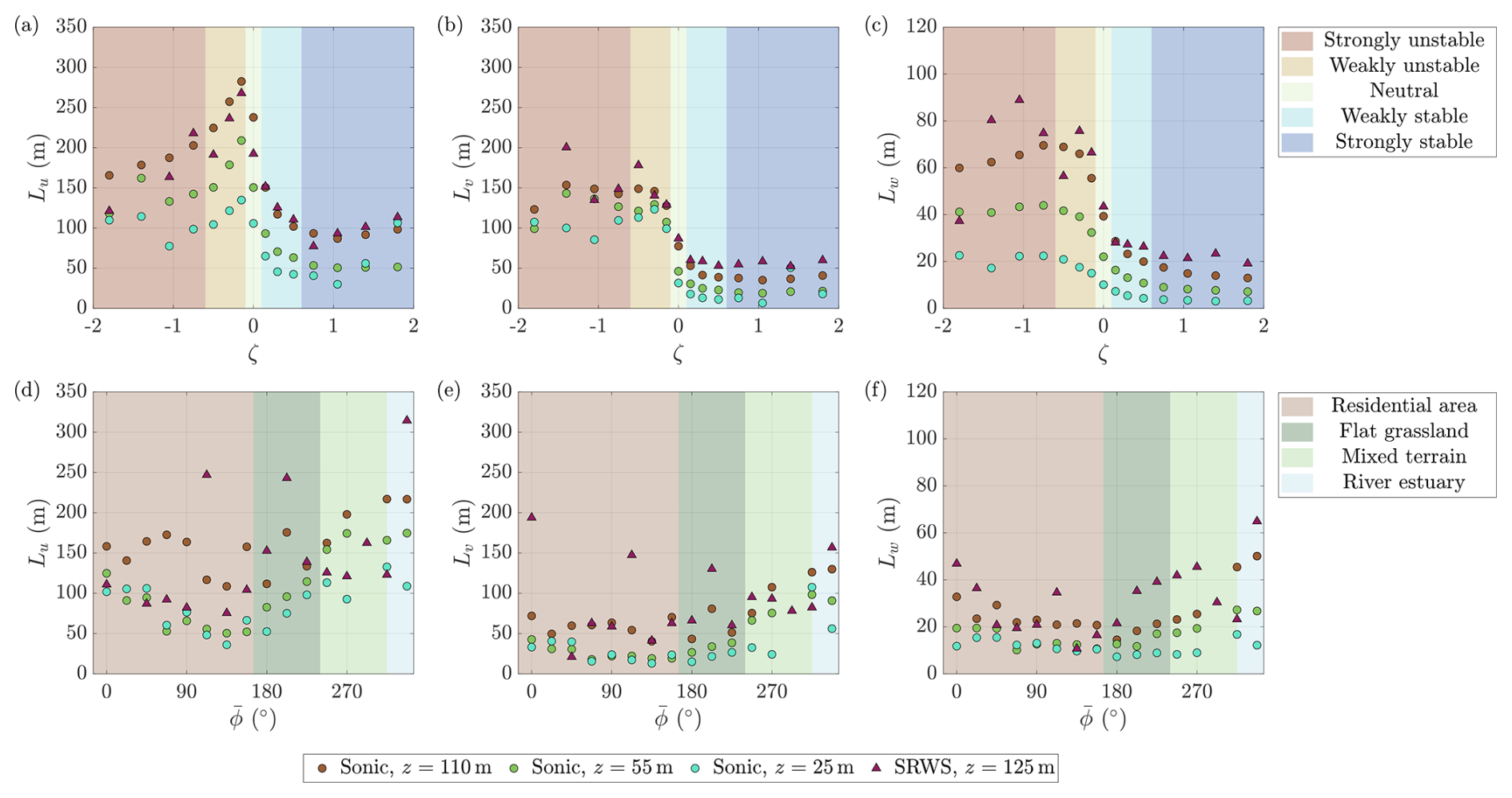
Figure 10 Median integral length scales derived from the auto-correlation function as a function of (a–c) atmospheric stability and (d–f) wind direction. Panels (c) and (f) use a reduced y-axis scale for the vertical length scale L_w for improved readability.

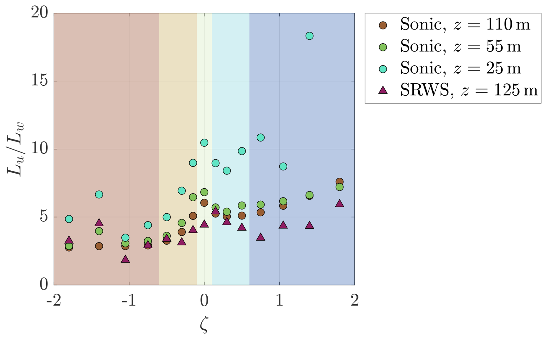
Figure 11 Ratio of along-wind to vertical integral length scales as a function of atmospheric stability. Background shading indicates the atmospheric-stability classes as labelled in Fig. 10a–c.

The dependence of the integral length scales on atmospheric stability and wind direction is illustrated in Fig. 10. Under neutral conditions, the integral length scales are within the ranges of 100 to 250 m for L_u, 30 to 100 m for L_v, and 10 to 50 m for L_w. From neutral to slightly unstable conditions, the length scales increase, consistent with enhanced turbulence generation due to buoyancy. Unexpectedly, this trend does not persist in the highly convective regime, which may be related to limitations of Taylor's hypothesis of frozen turbulence. The estimation of integral length scales from single-point temporal auto-correlation functions assumes that turbulent structures are advected past the measurement location without undergoing significant evolution. Under unstable stratification, buoyancy-driven turbulence may accelerate the temporal evolution of turbulent eddies, causing the measured auto-correlation functions to decay more rapidly. Consequently, the slightly smaller integral length scales estimated under highly unstable conditions may not necessarily reflect smaller turbulent structures but rather indicate departures from Taylor’s hypothesis of frozen turbulence. From neutral to slightly stable conditions, all length scales decrease substantially as buoyancy transitions from enhancing to suppressing turbulence. Under highly stable conditions, however, a slight increase in L_u and L_v is observed, which can be attributed to large-scale mesoscale motions increasingly captured within the 30 min averaging period. This effect is limited to the horizontal components, supporting the common assumption of quasi-two-dimensional mesoscale structures.

Figure 11 shows the ratio of the along-wind to the vertical length scales. Under unstable conditions, the ratio remains relatively constant between values of 2 and 6 but increases approximately by a factor of 2 towards neutral and even further under stable stratification. This trend reflects the deformation of turbulent eddies due to negative buoyancy and reduced vertical mixing under stable conditions, with the effect being most pronounced at lower measurement heights.

The variation in length scales with wind direction (Fig. 10d–f) is less systematic and generally weaker than the dependence on atmospheric stability. Nevertheless, a consistent increase in L_i is observed for wind directions $\stackrel{\mathrm{‾}}{\mathit{\varphi }}>\mathrm{180}$°, corresponding to flow over both flat terrain and from the estuary. Smaller length scales occur for $\stackrel{\mathrm{‾}}{\mathit{\varphi }}<\mathrm{180}$°, likely due to enhanced small-scale turbulence generated by the upstream built area.

4.2.2 Auto-spectra

The usable frequency range of the spectral estimates is assessed in Fig. 12. Figure 12a shows the ensemble-averaged horizontal wind speed spectra from the sonic and cup anemometers under neutral conditions. Residual high-frequency noise is present even after despiking the time series. When normalizing the frequencies by z U⁻¹, this noise may bias the estimates closer to the turbulence peak. To avoid this, the spectra are truncated prior to normalization and ensemble averaging. For the cup anemometers, a cut-off frequency of 0.3 Hz, corresponding to 0.6 f_N, is applied. The sonic spectra are truncated at 2 Hz for $z=\mathit{\{}\mathrm{55},\mathrm{110}\mathit{\}}\mathrm{m}$ and at 6 Hz for the instrument at z=25 m, which is from a different manufacturer.

A high level of agreement between sonic and cup spectra is observed up to approximately 0.07 Hz. At higher frequencies within the inertial subrange, the sonic spectra continue to follow the expected $fS\propto f^{-\mathrm{2}/\mathrm{3}}$ scaling, whereas the cup spectra exhibit pronounced high-frequency attenuation. This behaviour is attributed to spatial averaging associated with the cup geometry and temporal filtering due to the rotor inertia.

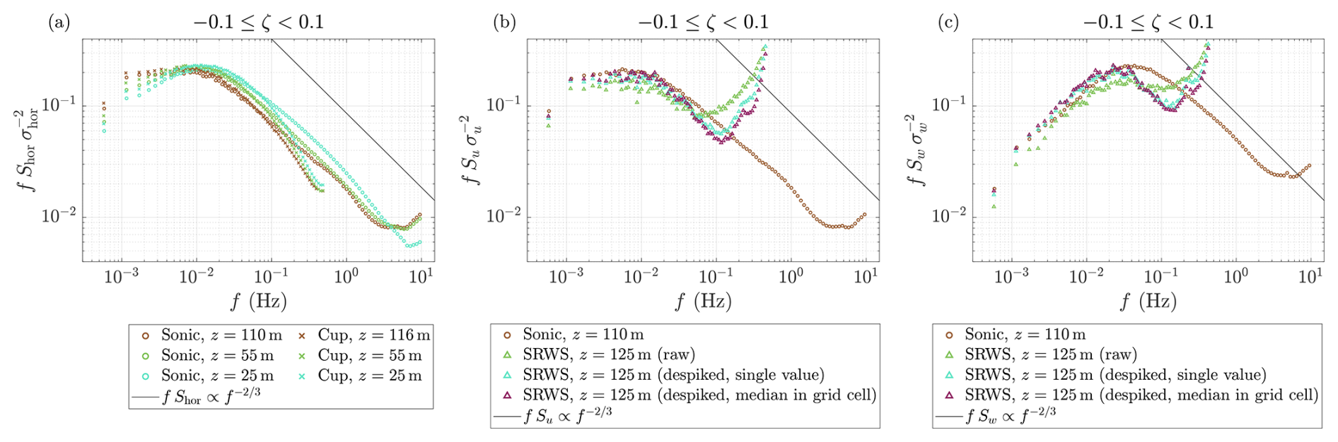
Figure 12 Turbulence spectra of (a) horizontal wind speed from sonic and cup anemometers, as well as (b) along-wind velocity and (c) vertical velocity from sonic anemometers and SRWS, all under neutral conditions.

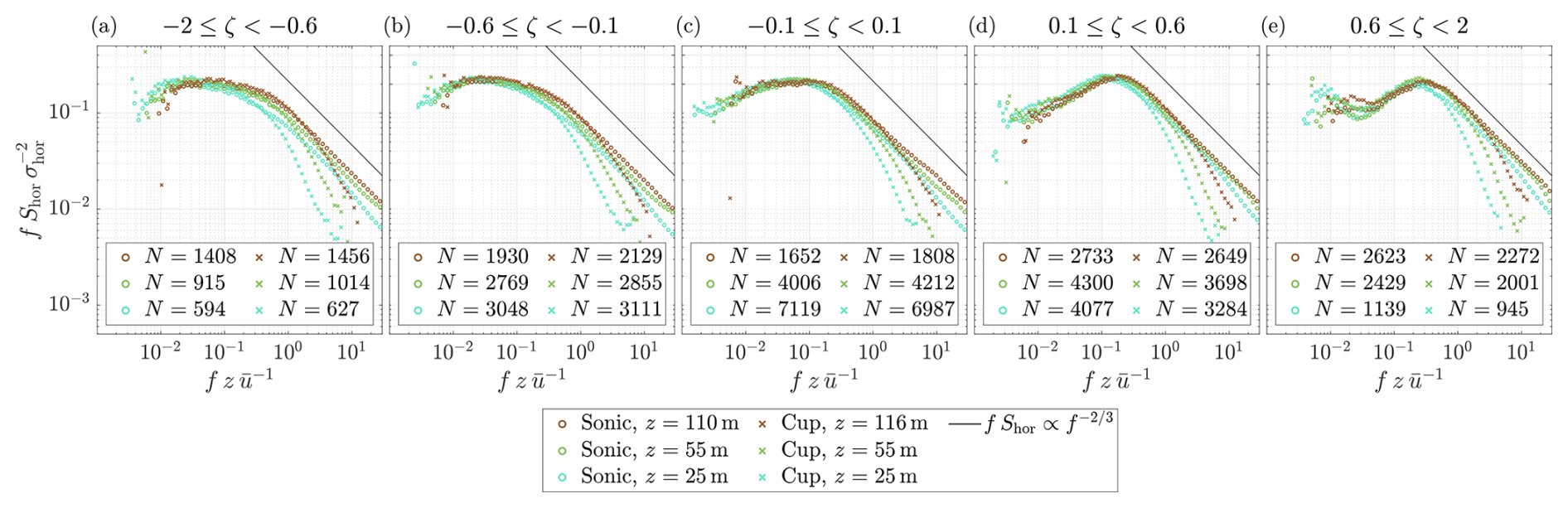
Figure 13 Ensemble-averaged horizontal wind speed spectra from sonic and cup anemometers under (a) highly unstable to (e) highly stable conditions.

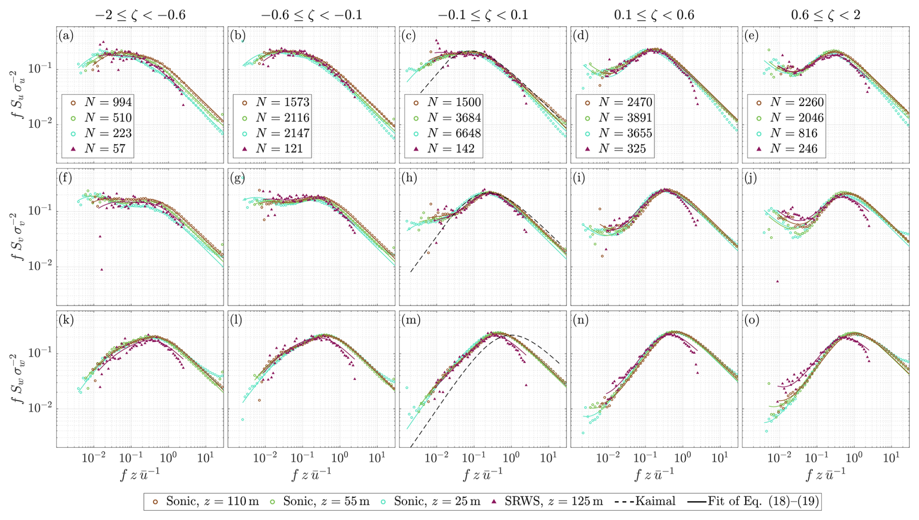
Figure 14 Ensemble-averaged (a–e) along-wind, (f–j) cross-wind, and (k–o) vertical velocity spectra from sonic anemometers and SRWS under highly unstable (left) to highly stable (right) conditions.

The normalized horizontal wind speed spectra from the sonic and cup anemometers are shown in Fig. 13 for five stability classes, plotted as a function of the reduced frequency. The number of samples N is indicated for each case in the legend. Under unstable conditions, the combined influence of shear- and buoyancy-driven turbulence results in a pronounced spectral plateau. As stability approaches neutral conditions, the plateau narrows due to the diminishing buoyancy contribution. Under stable stratification, the turbulence peak shifts towards higher frequencies as negative buoyancy suppresses the micro-scale turbulence and reduces the size of the coherent structures. Simultaneously, low-frequency contributions emerge, likely related to mesoscale motions.

Aside from the high-frequency attenuation, the spectra from sonic and cup anemometers show good agreement at corresponding heights. The largest discrepancies occur within the spectral gap under highly stable conditions, where the sonic spectra indicate slightly higher spectral energy.

Figure 12b and c compare along-wind and vertical spectra under neutral conditions obtained from the sonic anemometer at a height of 110 m and the SRWS at the bow-tie centre (z=125 m). The raw lidar time series were found to be relatively noisy, leading to artificial spectral energy above approximately 0.06 Hz. After despiking, the usable frequency range extends to about 0.1 Hz. Additional smoothing is achieved by extracting the median of five neighbouring values within a grid cell rather than a single sample, which, at the bow-tie centre, corresponds to a trajectory length of approximately 4.7 m.

Similar to the cup anemometer results, the SRWS spectra display high-frequency attenuation, primarily due to the lidars' finite probe volume, starting around 0.04 Hz for both velocity components shown in Fig. 12. While the along-wind spectrum is only affected in the inertial subrange, the spectral peak of the vertical component cannot entirely be resolved by the SRWS.

The resulting velocity spectra are presented in Fig. 14 for the three sonic anemometers and the SRWS recordings in the bow-tie centre. Under unstable conditions, the along- and cross-wind spectra exhibit a distinct spectral plateau. The plateau is more pronounced for the cross-wind component and, unlike for the along-wind velocity, does not persist under neutral conditions. Instead, a spectral gap becomes apparent in the neutral f S_v estimate, consistent with offshore observations by Cheynet et al. (2018) and Patel et al. (2026). In further agreement with Cheynet et al. (2018), the spectral gap is located at reduced frequencies of approximately $\mathrm{5}\times {\mathrm{10}}^{-\mathrm{3}}$ to $\mathrm{2}\times {\mathrm{10}}^{-\mathrm{2}}$ under slightly stable conditions and $\mathrm{2}\times {\mathrm{10}}^{-\mathrm{2}}$ to $\mathrm{5}\times {\mathrm{10}}^{-\mathrm{2}}$ under highly stable conditions. The spectral gap reaches deeper for the cross-wind spectra than for the along-wind component. Its depth and position vary with height, with higher elevations exhibiting a shallower gap shifted towards higher frequencies, consistent with observations by Larsén et al. (2016) at the coastal Høvsøre site.

For the vertical velocity component, the spectral plateau is less distinct but still observable under convective conditions. Under neutral conditions, the w spectra follow the basic f S_i(n)∝f¹ and $f{S}_i\left(n\right)\propto f^{-\mathrm{2}/\mathrm{3}}$ scaling, as neither a plateau nor a low-frequency contribution is present. For the 30 min averaging period considered here, a clearly defined spectral gap is not observed under stable conditions, although indications are present at reduced frequencies below $\mathrm{2}\times {\mathrm{10}}^{-\mathrm{2}}$, consistent with Larsén et al. (2016) and Cheynet et al. (2018).

The SRWS spectra appear less smooth due to the smaller sample size. However, they seem to capture the main spectral features, including the plateau, the turbulence peak, and the spectral gap, for most cases. Furthermore, the depth of the spectral gap follows the height-dependent trend observed across the sonic measurements. For the along-wind component, deviations from the sonic results are limited to the inertial subrange, where attenuation in the SRWS spectra leads to an underestimation of spectral energy. The spatial averaging effect is more severe for the v and w components, where both the magnitude and position of the turbulence peak are distorted. In the cross-wind spectra, this is the case under stable conditions only, whereas the vertical turbulence peaks are affected across all stability regimes.

In addition to the measurements, Fig. 14 includes least-square fits of the empirical turbulence models (Eqs. 18–19) together with the IEC parametrization of the Kaimal spectrum for neutral conditions. For the horizontal components, the Kaimal spectrum matches the peak and inertial subrange but underestimates the low-frequency energy due to the presence of the spectral plateau in u and the mesoscale contributions in v. For the vertical component, the overall spectral shape is captured reasonably well, although the peak frequency is shifted by approximately n≈0.5. The peak estimated around a reduced frequency of around $\mathrm{5}\times {\mathrm{10}}^{-\mathrm{1}}$ is, however, consistent with the observations of Cheynet et al. (2018).

The pointed–blunt model (Eq. 18) provides a good representation of the spectral plateau through a double-peak, resulting in accurate fits for unstable and neutral conditions. The pointed model with mesoscale contribution (Eq. 19) used under stable conditions captures the spectral gap well, except in Fig. 14j, where the particularly narrow gap at 25 and 55 m cannot be reproduced accurately. The coefficients derived from fitting the turbulence models to the observations are provided in Appendix A as functions of atmospheric stability.

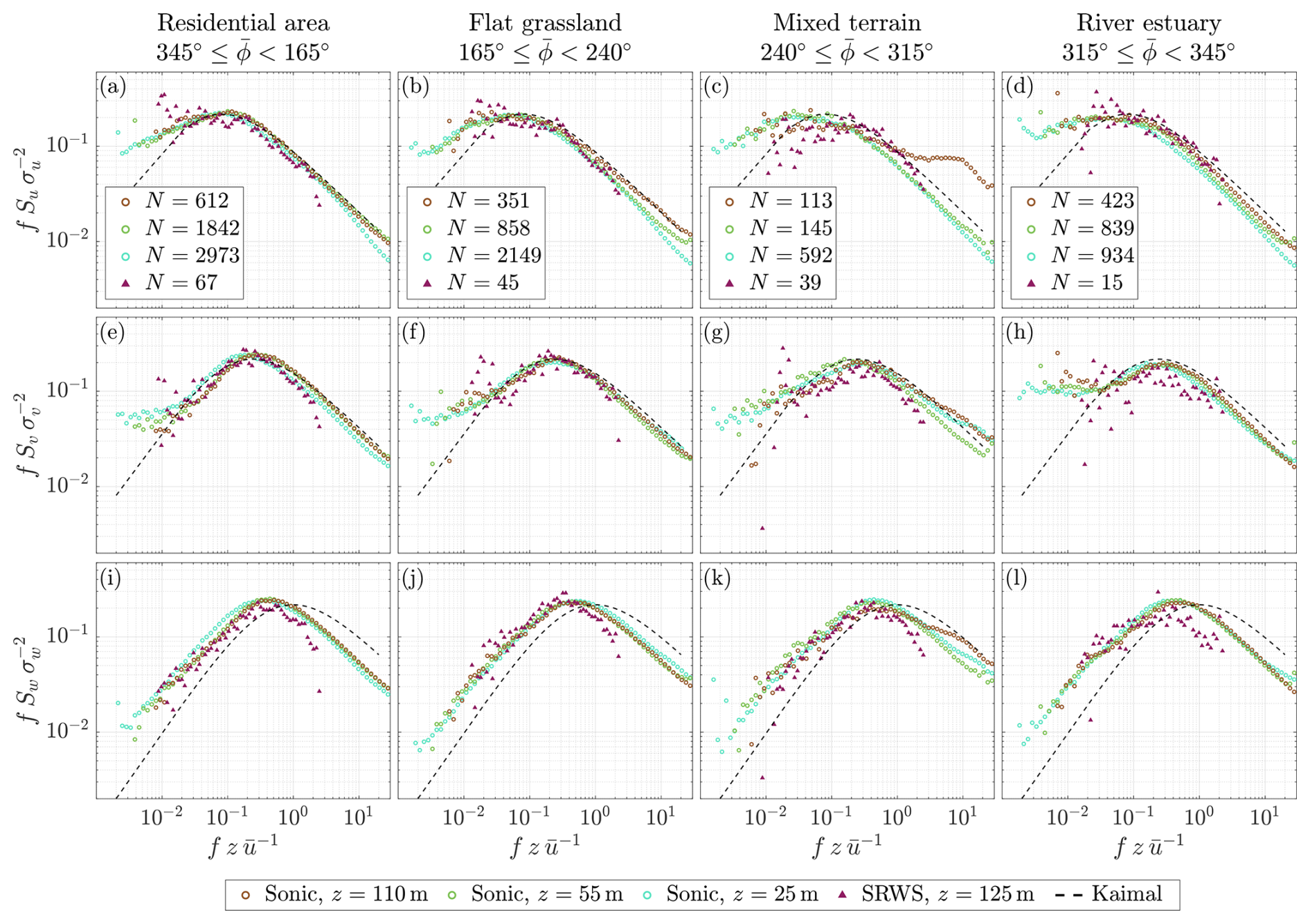
Figure 15 Ensemble-averaged (a–d) along-wind, (e–h) cross-wind, and (i–l) vertical velocity spectra from sonic anemometers and SRWS under neutral conditions for four wind-direction sectors.

The low-frequency contribution captured within the 30 min averaging window is generally well approximated by the $S_i\left(n\right)\propto f^{-\mathrm{5}/\mathrm{3}}$ scaling. Under highly stable conditions, the u and v spectra suggest the presence of a secondary peak at frequencies below the spectral gap, which is not represented by the turbulence model. Similar observations were reported by Caughey (1977) and Cheynet et al. (2018) near the Brunt–Väisälä frequency and attributed to wave-like motions in stable stratification. A more detailed investigation of this feature would require longer averaging periods to resolve lower-frequency contributions.

The auto-spectral estimates presented in Figs. 12–14 are ensemble averages over all wind directions that are not affected by turbine or mast wake interference. Prior to ensemble averaging, each spectrum is normalized by its corresponding variance to reduce the influence of directional differences in turbulence intensity. However, as shown in Fig. 10d–f, the integral length scales vary with wind direction, indicating that the spectral shape is also expected to differ based on the upstream terrain. This effect is examined in Fig. 15, which presents normalized spectra under neutral conditions for four wind-direction sectors with contrasting terrain characteristics. As the upstream roughness decreases from Fig. 15a (residential area) to Fig. 15d (river estuary), the low-frequency energy increases, causing the along-wind turbulence peak around n=0.1 to gradually broaden into a spectral plateau. This behaviour is consistent with the corresponding increase in the integral length scales discussed previously. A similar increase in low-frequency energy is observed in the cross-wind spectra, whereas the vertical velocity spectra are comparatively insensitive to the upstream terrain. Overall, the sonic anemometer and SRWS spectra exhibit similar trends across the different sectors. Some estimates, however, such as the sonic spectrum at z=110 m in Fig. 15c, show increased uncertainty due to the smaller number of available samples.

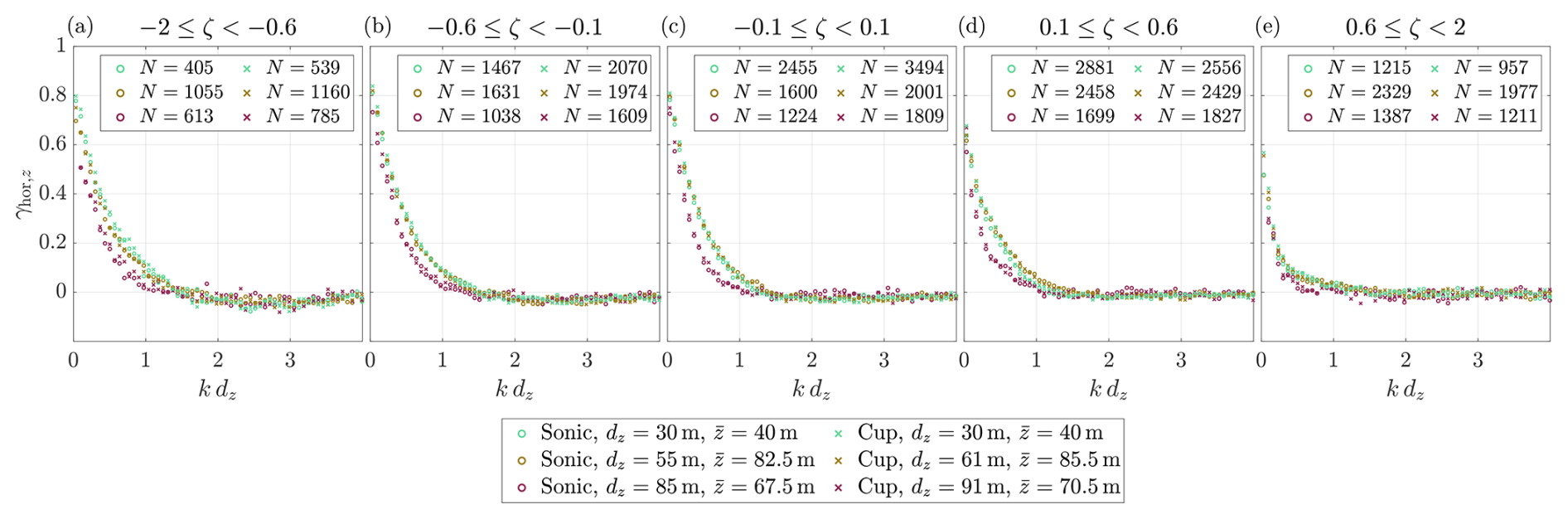
Figure 16 Vertical co-coherence of horizontal wind speed from sonic and cup anemometers under (a) highly unstable to (e) highly stable conditions.

Figure 17 Vertical co-coherence of (a–e) along-wind, (f–j) cross-wind, and (k–o) vertical velocity from sonic anemometers and SRWS at comparable separations and measurement heights under highly unstable (left) to highly stable (right) conditions.

4.3 Spectral co-coherence

4.3.1 Vertical separations

Vertical coherence of the horizontal wind speed is evaluated along the meteorological mast using both sonic and cup anemometers. The ensemble-averaged results, shown in Fig. 16, are expressed as a function of the normalized wavenumber k d_z. The coherence estimates are consistent across all separations and stability classes, indicating that they are largely unaffected by attenuation in the inertial subrange of the cup anemometer spectra. This can partially be explained by the fact that attenuation occurs at f>0.07 Hz, whereas the coherence of the horizontal wind speed decays at normalized wavenumbers below 1.5. Contributions from frequencies above 0.07 Hz can only be reflected at such low values of k d_z at relatively high mean wind speeds of $\overline{u}>\mathrm{8.8}\mathrm{m}{\mathrm{s}}^{-\mathrm{1}}$ for d_z=30 m, $\overline{u}>\mathrm{17.9}\mathrm{m}{\mathrm{s}}^{-\mathrm{1}}$ for d_z=61 m, and $\overline{u}>\mathrm{26.7}\mathrm{m}{\mathrm{s}}^{-\mathrm{1}}$ for d_z=91 m. In addition, spatial averaging effects may partially cancel when the cross-spectrum between two points is normalized by the corresponding auto-spectra, as discussed by Cheynet et al. (2016a) for coherence estimates derived from dual-lidar measurements.

In the present study, a direct comparison between sonic- and lidar-based coherence estimates is challenging due to differences in measurement height. For instance, the sonic estimate for d_z=30 m corresponds to an average height of $\overline{z}=\mathrm{40}\mathrm{m}$, whereas the lowest SRWS estimate is available at $\overline{z}=\mathrm{70}\mathrm{m}$. The closest correspondence is found between the sonic separation of d_z=55 m at $\overline{z}=\mathrm{82.5}\mathrm{m}$ and the SRWS estimate between the first to seventh grid cell along the vertical scan line (Fig. 6b), yielding d_z=60 m at $\overline{z}=\mathrm{85}\mathrm{m}$.

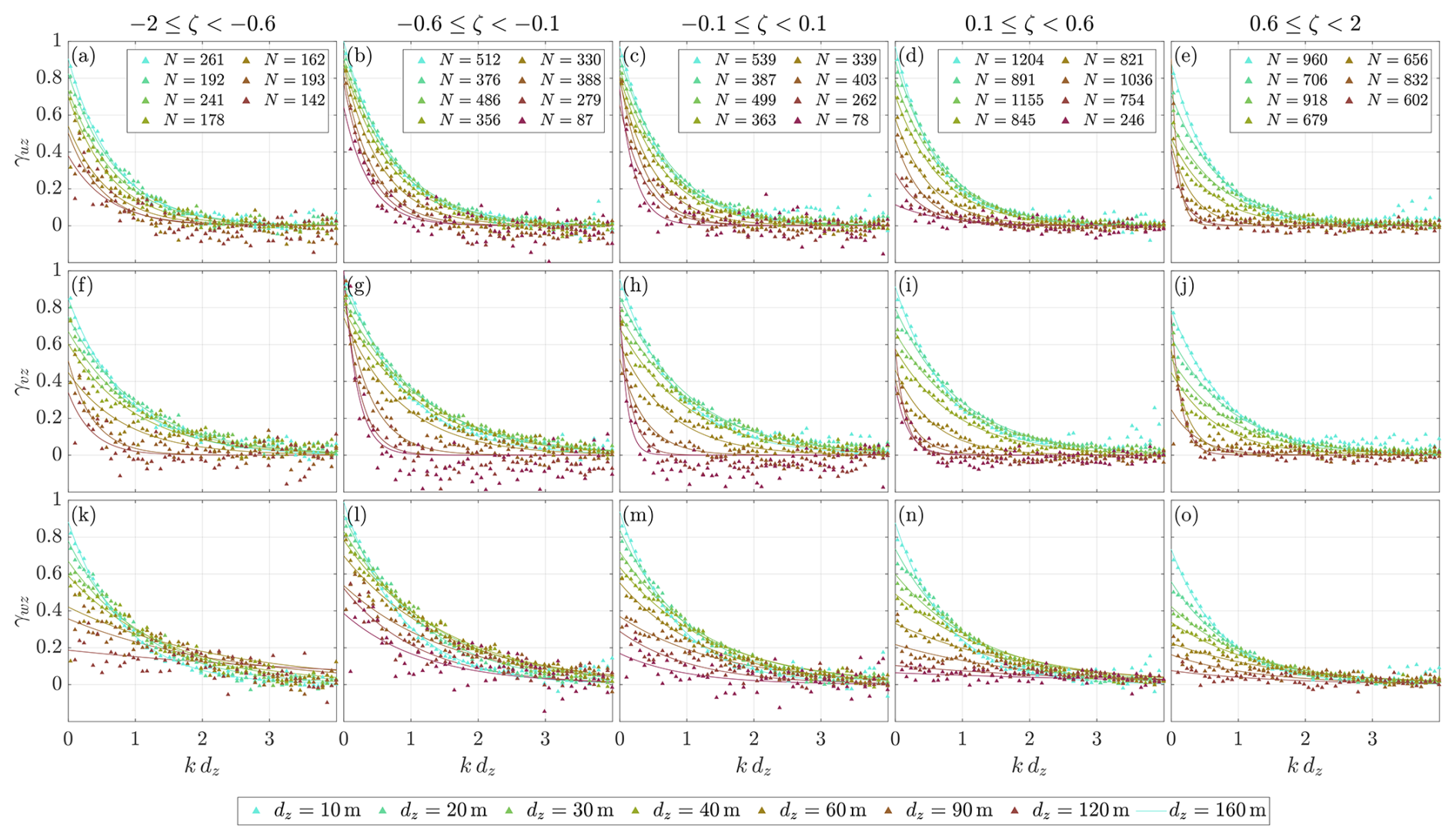
Figure 18 Vertical co-coherence of (a–e) along-wind, (f–j) cross-wind, and (k–o) vertical velocity from SRWS for separations ranging from 10 to 160 m under highly unstable (left) to highly stable (right) conditions and average heights of $\mathrm{110}\mathrm{m}\le \overline{z}\le \mathrm{140}\mathrm{m}$. The 160 m separation is omitted for $\left|\mathit{\zeta }\right|>\mathrm{0.6}$ due to high uncertainty associated with a limited sample size.

The corresponding coherence estimates are compared in Fig. 17. The horizontal velocity components exhibit a high agreement across all stability classes. Significant deviations are observed only for the along-wind component under highly unstable conditions (Fig. 17a), where the limited number of samples increases the uncertainty in the SRWS estimate.

For the vertical velocity component, however, the SRWS predicts systematically lower coherence, approximately by a factor of 2 compared to the sonic estimates. Part of this discrepancy may be attributed to the slight difference in separation distance (5 m), as γ_wz is typically more sensitive to d_z than the horizontal components. The remaining difference may reflect either an underestimation by the SRWS or an overestimation by the sonic measurements. The sonic-based coherence aligns well with results reported by Cheynet et al. (2018) for d_z=40 m at the FINO1 offshore platform. This agreement may suggest that the sonic anemometers' γ_wz in Fig. 17 is overestimated, as a 60 m separation onshore would be expected to exhibit lower coherence than a 40 m spacing offshore. As reported by Cheynet et al. (2016a), a reduction in the lidar-based coherence estimates due to spectral attenuation related to volume-averaging is unlikely because the cross-spectra are normalized by the correspondingly attenuated auto-spectra. Any residual influence is expected to be negligible for normalized wavenumbers below 1, as the attenuation primarily affects frequencies above 0.04 Hz. For a separation of 60 m, these frequencies correspond to k d_z<1 only for mean wind speeds exceeding 15 m s⁻¹, which are rarely encountered in the present dataset.

The velocity reconstruction and coherence estimation based on the SRWS scans may, however, introduce additional decorrelation effects that are specific to the w component. Due to its greater spatial variability within the finite measurement volumes, the vertical velocity is more sensitive than the horizontal components to departures from the assumptions underlying the velocity reconstruction. Furthermore, the correction for the time lag between the vertically separated extraction points relies on Taylor's hypothesis of frozen turbulence and is thus expected to be less accurate for the vertical velocity component because of the more rapid temporal evolution of vertical motions. Both effects may contribute to reducing the correlation between the SRWS-derived vertical velocity time series at different heights. A conclusive assessment would require additional γ_wz estimates at comparable heights and separations.

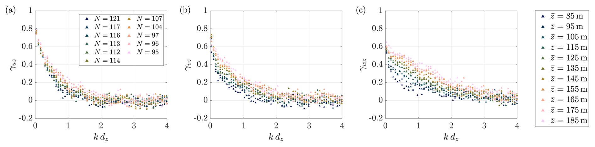
Figure 19 Vertical co-coherence of (a) along-wind, (b) cross-wind, and (c) vertical velocity from SRWS as a function of the average measurement height $\overline{z}$ for a vertical separation of d_z=60 m under neutral conditions.

Despite the differences between instruments, the coherence of the vertical turbulence exhibits consistent trends with atmospheric stability. From unstable to stable conditions, coherence decreases, reflecting the reduction in turbulent length scales. For the horizontal components, this is expressed through a steeper decay and a moderate reduction in coherence at k=0. For the vertical component, the reduction is more pronounced, leading to substantially lower intercepts with the y axis under stable conditions.

Figure 18 presents the SRWS-based coherence estimates for separations between 10 and 160 m along the vertical line of the scan. To obtain meaningful averages as a function of stability and separation distance, the ensembles are restricted to estimates obtained at comparable measurement heights of $\mathrm{110}\mathrm{m}\le \overline{z}\le \mathrm{140}\mathrm{m}$. The fitted curves correspond to Eq. (22). The model provides an accurate representation of the observations while allowing for ${\mathit{\gamma }}_{iz}(k=\mathrm{0})<\mathrm{1}$.

According to the Davenport model (Eq. 21), coherence scales with $f{d}_z{\overline{u}}^{-\mathrm{1}}$, implying that all estimates should collapse into a single curve when plotted against k d_z. This is not observed, suggesting a stronger dependency on d_z. Additionally, coherence is affected by the measurement height, which is not accounted for by the Davenport model. The height dependence of the vertical coherence is examined in Fig. 19 for a fixed separation distance of d_z=60 m and neutral conditions. A reduction in coherence with decreasing height is observed for all wind components while being most pronounced for the vertical velocity. The coherence of the along-wind turbulence appears to be least sensitive to $\overline{z}$ and exhibits a noticeable dependence only at normalized wavenumbers k d_z>0.25.

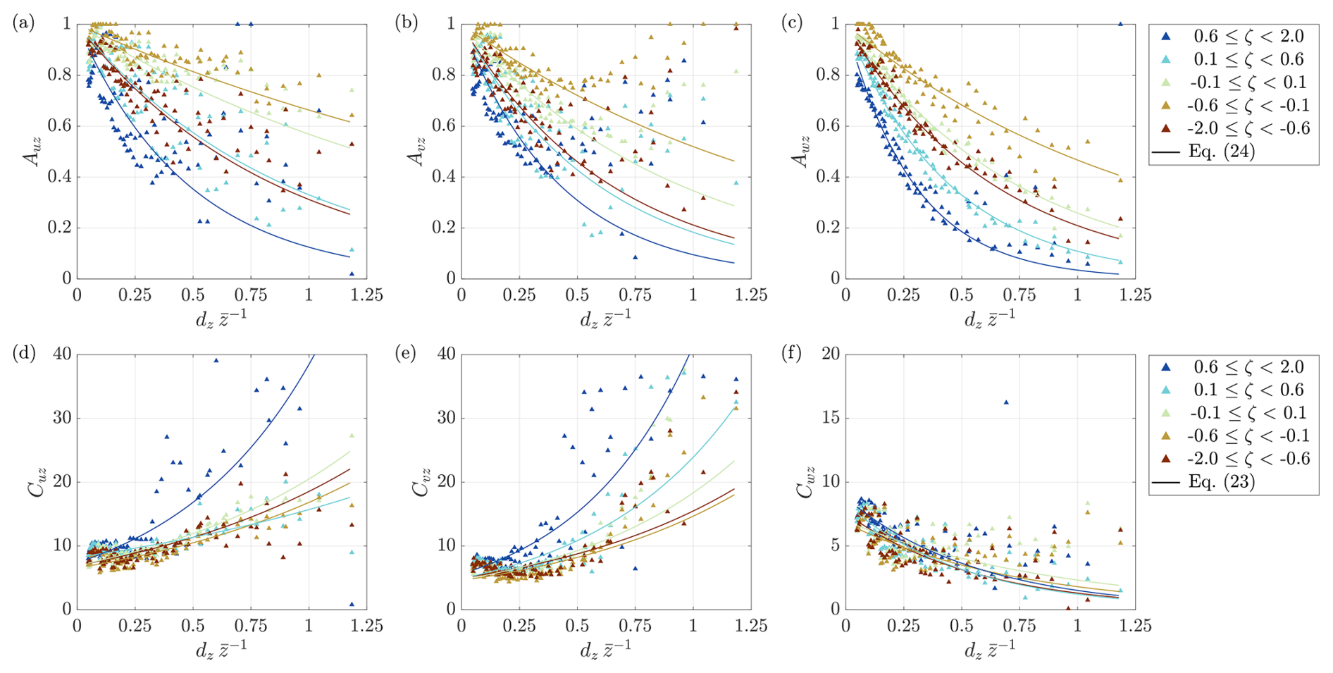
Figure 20 Fitted (a–c) scaling coefficients and (d–f) decay coefficients of vertical coherence based on Eq. (22), including exponential regressions.

To account for the combined influence of measurement height and separation distance, the model coefficients A and C in Eq. (22) are fitted for a wide range of combinations across the bow-tie pattern. The resulting coefficients are shown in Fig. 20 as a function of the normalized separation $d_z{\overline{z}}^{-\mathrm{1}}$. For small values of $d_z{\overline{z}}^{-\mathrm{1}}$, the scaling coefficient A approaches 1, corresponding to identity coherence at k=0. With increasing separation or decreasing height, A decreases approximately exponentially. The exponential formulation in Eq. (24) provides an accurate fit to A_w. Greater scatter is observed for the horizontal components, particularly for $d_z{\overline{z}}^{-\mathrm{1}}>\mathrm{0.5}$.

Bowen et al. (1983) established a linear relationship between the decay coefficient C and $d_z{\overline{z}}^{-\mathrm{1}}$ based on propeller anemometer measurements within 20 m over open rural terrain. In the present results, a better representation is achieved using the two-parameter exponential function given in Eq. (23).

Combining the derived parameterizations of A and C with the basic coherence model yields the three-parameter model given in Eq. (25). The corresponding model coefficients are summarized in Appendix B as a function of atmospheric stability.

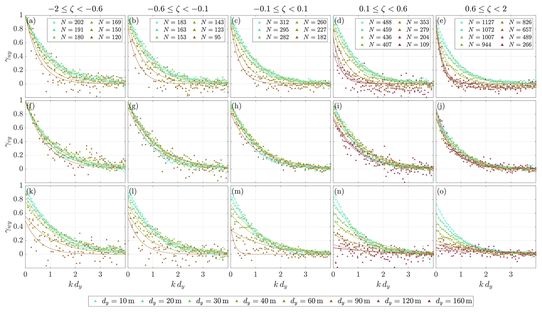
Figure 21 Lateral co-coherence of (a–e) along-wind, (f–j) cross-wind, and (k–o) vertical velocity from SRWS for separations ranging from 10 to 160 m under highly unstable (left) to highly stable (right) conditions and a measurement height of 125 m. The 120 and 160 m separations are omitted for ζ<0.1 due to high uncertainty associated with a limited sample size.

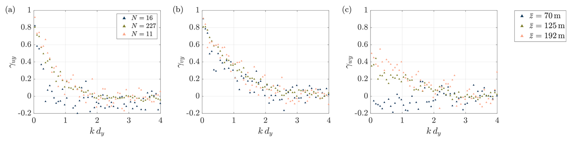
Figure 22 Lateral co-coherence of (a) along-wind, (b) cross-wind, and (c) vertical velocity from SRWS as a function of the average measurement height $\overline{z}$ for a lateral separation of d_z=60 m under neutral conditions.

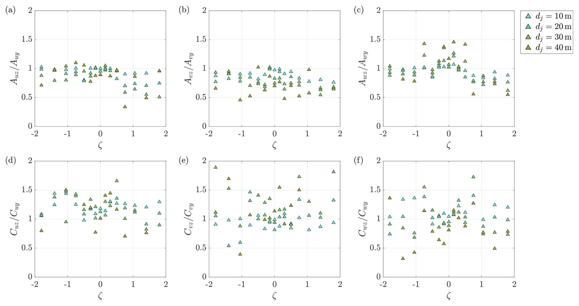
Figure 23 Ratio of vertical to lateral (a–c) scaling coefficients and (d–f) decay coefficients for separations of d_j=10 to 40 m and mean heights of $\overline{z}=\mathrm{120}$ to 130 m.

4.3.2 Lateral separations

The lateral coherence derived from the SRWS scans is shown in Fig. 21. The reduction in turbulent length scales from unstable to stable conditions is reflected in the lateral coherence. However, the associated reduction in coherence is less pronounced than for vertical separations. This behaviour is consistent with the integral length scales (Fig. 10), which indicate that turbulent structures are more highly compressed in the vertical than in the lateral direction. As a result, laterally separated points are less sensitive to stability effects than vertically separated ones. Unlike for the vertical direction, the lateral coherence of the cross-wind component γ_vy appears to scale relatively well with the normalized wavenumber k d_y.

To obtain meaningful ensemble averages, the lateral coherence estimates shown in Fig. 21 are restricted to a measurement height of 125 m, corresponding to estimates obtained along the horizontal segment of the bow-tie pattern. For lateral separations between 10 and 90 m, one additional estimate is available both above and below this height from the diagonal segments connecting to the vertical line, as illustrated in Fig. 6. For d_y=60 m, these estimates are located at $\overline{z}=\mathrm{70}\mathrm{m}$ and $\overline{z}=\mathrm{192}\mathrm{m}$ and are compared to the $\overline{z}=\mathrm{125}\mathrm{m}$ estimate in Fig. 22. Although only three measurement heights are available, and the estimates at the lowest and highest elevations are associated with relatively large uncertainty, a reduction in lateral coherence with decreasing measurement height is evident. Consistent with the vertical coherence results (Fig. 19), the height sensitivity is most pronounced for γ_wy. At $\overline{z}=\mathrm{70}\mathrm{m}$, the vertical velocity is quasi-incoherent across the d_y=60 m separation.

A direct comparison between vertical and lateral coherence is provided in Fig. 23 in terms of the ratios of the fitted scaling and decay coefficients A and C. To ensure comparability, only estimates at similar heights within the range of $\overline{z}=\mathrm{120}$ to 130 m are included. The analysis is further restricted to separations up to 40 m, as the representative height $\overline{z}$ becomes less meaningful for larger vertical spacings.

While no clear trend is observed for $C_{iz}/C_{iy}$, the ratio of the scaling coefficient A decreases slightly under stable conditions, suggesting that the vertical coherence reduces more rapidly than the lateral coherence. This observation is consistent with the flattening of turbulent structures caused by the suppression of vertical mixing under stable stratification.

The combination of slightly smaller decay coefficients and larger scaling coefficients for lateral separations indicates that lateral coherence generally exceeds vertical coherence.

5 Conclusions

Wind velocity measurements from a near-coastal site in northern Germany are analysed to derive single- and two-point turbulence characteristics. The dataset comprises 20 months of sonic and cup anemometer observations at three levels along a 116 m meteorological mast, complemented by approximately 90 d of SRWS measurements. The SRWS system consists of three continuous-wave lidars executing synchronized scans in a bow-tie pattern. After quality control and filtering, about 7500 h of sonic, 8000 h of cup, and 700 h of lidar data remain available. Three-dimensional velocity time series from the sonics and reconstructed from the SRWS measurements are used to estimate auto-spectra and spatial co-coherence. In addition, single- and two-point spectra of the horizontal wind speed are derived from both sonic and cup anemometers.

The auto-spectral estimates from the different sensors show remarkable agreement at low and intermediate frequencies. The sonic anemometers, sampling at 20 Hz, provide reliable spectra up to approximately 2 to 6 Hz before measurement noise affects the inertial subrange. Although the cup anemometers operate at 1 Hz, spectral attenuation becomes apparent above 0.07 Hz due to spatial and inertial averaging. The attenuation is most critical under stable conditions, where it occurs close to the turbulence peak, which nevertheless remains fully resolved.

Lidar-based velocity time series are extracted at the centre of the bow-tie scan, where the trajectory intersects twice per cycle, yielding an effective sampling rate of 1 Hz. Spatial averaging associated with the lidar probe volume leads to attenuation at frequencies above 0.04 Hz. This allows the turbulence peak of the along-wind component to be captured across all stability regimes. The cross-wind spectra are well reproduced under unstable and neutral conditions, whereas under stable stratification the attenuation influences the appearance of the turbulence peak. The vertical spectra are affected even under convective conditions. For the present SRWS configuration, spectral estimates should therefore be interpreted with caution in the absence of a sonic reference. At low frequencies, however, strong agreement with the sonic measurements is observed for all velocity components and stability classes.

The observed spectral attenuation has no noticeable influence on coherence estimates, as it primarily occurs at frequencies beyond those governing coherence decay. Furthermore, it may partly cancel when normalizing cross-spectra by auto-spectra. Accordingly, vertical coherence derived from cup anemometers and the SRWS system agrees well with the sonic-based estimates for the horizontal components. For the vertical component, a systematic discrepancy is observed, although it remains unclear whether this reflects an overestimation by the sonics or an underestimation by the lidars.

The bow-tie scanning strategy proves highly suitable for coherence analysis, as it enables flexible estimation of vertical and lateral coherence across a wide range of separations and heights, which is challenging to achieve with conventional mast-based measurements.

In this work, all spectral estimates are classified according to atmospheric stability derived from sonic heat flux measurements. The resulting annual and diurnal stability distributions exhibit characteristic patterns for onshore conditions. A sufficient number of samples spanning highly unstable to highly stable regimes are available across a wide range of wind speeds and directions, enabling a comprehensive assessment of stability effects on turbulence characteristics.

Under convective conditions, integral length scales of L_u=100 to 300 m, L_v=100 to 200 m, and L_w=20 to 100 m are observed between heights of 25 and 125 m, reflecting the combined influence of shear- and buoyancy-driven turbulence production. This contribution is also evident in the auto-spectra, which exhibit a broadened peak in the vertical component and a wide spectral plateau in the horizontal components. The pointed–blunt model, approximating the plateau with a double peak, provides an accurate description across all velocity components.

From unstable to slightly stable conditions, the integral length scales decrease substantially to approximately L_u=40 to 110 m, L_v=10 to 50 m, and L_w=4 to 30 m, accompanied by a shift in spectral energy towards higher frequencies. Under neutral conditions, a spectral plateau persists only in the along-wind component, whereas the cross-wind and vertical spectra exhibit distinct peaks that are well described by the Kaimal model. However, deviations from the IEC formulation are observed in the low-frequency range of the cross-wind spectrum, which indicates the presence of a spectral gap.

Under stable stratification, the spectral gap becomes more pronounced as additional low-frequency energy emerges in the horizontal components, potentially related to mesoscale motions. This contribution is also reflected in slightly increased integral length scales of L_u=50 to 120 m and L_v=15 to 60 m. The vertical spectra are only marginally affected due to the predominantly two-dimensional nature of mesoscale motions. A spectral representation combining a turbulence peak with a $S_i\left(n\right)\propto f^{-\mathrm{5}/\mathrm{3}}$ scaling at low frequencies provides a satisfactory description under stable conditions.

Consistent behaviour is observed for spatial coherence, which decreases from unstable to stable conditions as turbulent structures reduce in size. Lateral coherence is systematically higher than vertical coherence, particularly under stable conditions.

A modified version of the Davenport coherence model that enables γ_ij(0)<1 accurately captures the coherence decay for all velocity components. Significant deviations from the classical $f{d}_j{\overline{u}}^{-\mathrm{1}}$ scaling are observed, as coherence depends more strongly on separation distance and is additionally influenced by measurement height. By introducing exponential relationships between the model coefficients and the normalized separation $d_j{\overline{z}}^{-\mathrm{1}}$, a three-parameter coherence model is established. While these exponential relationships provide accurate fits to the model parameters for the vertical velocity, increased scatter and deviations are observed for the horizontal components at $d_j{\overline{z}}^{-\mathrm{1}}>\mathrm{0.5}$. The reduced accuracy at large normalized separations can primarily be attributed to the low data availability resulting from the limited size of the SRWS bow-tie pattern. The available measurements therefore support an application of the proposed coherence model for normalized separations of $d_j{\overline{z}}^{-\mathrm{1}}\le \mathrm{0.5}$. Additional measurements at larger separations are recommended for assessing and improving the model accuracy for the horizontal velocity components beyond this range.

The resulting turbulence and coherence model parameters are provided as functions of atmospheric stability in Appendices A and B, respectively, and may serve as input for the generation of synthetic wind fields under non-neutral atmospheric conditions. Future work could build on these results by investigating how the observed stability-dependent variation in turbulence characteristics influences the dynamic response and loading of wind turbines. In addition, the measured spectra provide a valuable basis for a comparison with the uniform shear model (Syed and Mann, 2024) under different atmospheric-stability conditions. Further research could investigate methods for estimating lateral coherence from in situ measurements of vertical coherence, enabling a more comprehensive characterization of atmospheric turbulence with limited measurement equipment.

Appendix A: Proposed turbulence model and fitted coefficients

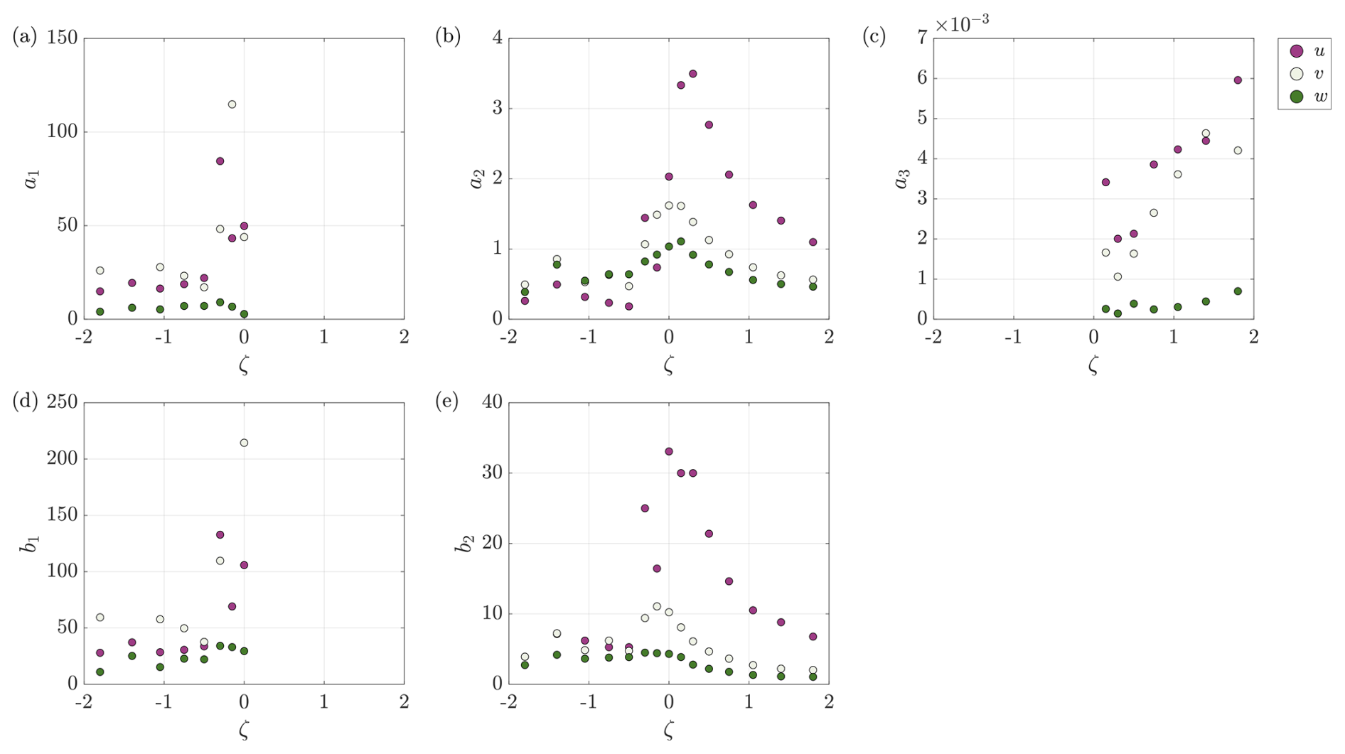
The turbulent auto-spectra are described using the pointed–blunt model (Cheynet et al., 2018) under neutral and unstable atmospheric conditions,

$$\begin{array}{}\text{(A1)}& {\displaystyle \frac{f{S}_i\left(n\right)}{{\mathit{\sigma }}_i^{\mathrm{2}}}}={\displaystyle \frac{a_{\mathrm{1}}^{i}n}{{\left(\mathrm{1}+b_{\mathrm{1}}^{i}n\right)}^{\mathrm{5}/\mathrm{3}}}}+{\displaystyle \frac{a_{\mathrm{2}}^{i}n}{\mathrm{1}+b_{\mathrm{2}}^i{n}^{\mathrm{5}/\mathrm{3}}}},\end{array}$$

and by the pointed model with mesoscale contribution for stable stratification:

$$\begin{array}{}\text{(A2)}& {\displaystyle \frac{f{S}_i\left(n\right)}{{\mathit{\sigma }}_i^{\mathrm{2}}}}={\displaystyle \frac{a_{\mathrm{2}}^{i}n}{\mathrm{1}+b_{\mathrm{2}}^i{n}^{\mathrm{5}/\mathrm{3}}}}+a_{\mathrm{3}}^i{n}^{-\mathrm{2}/\mathrm{3}}.\end{array}$$

The model coefficients, obtained from least-square fits to the sonic anemometer measurements at a height of 110 m, are presented in Fig. A1 and summarized in Tables B1–B3.

Figure A1 Empirical model coefficients for computation of turbulent auto-spectra of the along-wind, cross-wind, and vertical velocity components. Values are obtained from least-square fits of Eqs. (A1)–(A2) to the sonic anemometer data at z=110 m.

Appendix B: Proposed coherence model and fitted coefficients

The spatial coherence across both vertical and lateral separations is expressed as

$$\begin{array}{}\text{(B1)}& {\mathit{\gamma }}_{ij}\left(k{d}_j\right)=\text{exp}\left[-{\displaystyle \frac{k{d}_j}{\mathrm{2}\mathit{\pi }}}{c}_{\mathrm{1}}^{ij}\text{exp}\left(c_{\mathrm{2}}^{ij}{\displaystyle \frac{d_j}{\overline{z}}}\right)-c_{\mathrm{3}}^{ij}{\displaystyle \frac{d_j}{\overline{z}}}\right].\end{array}$$

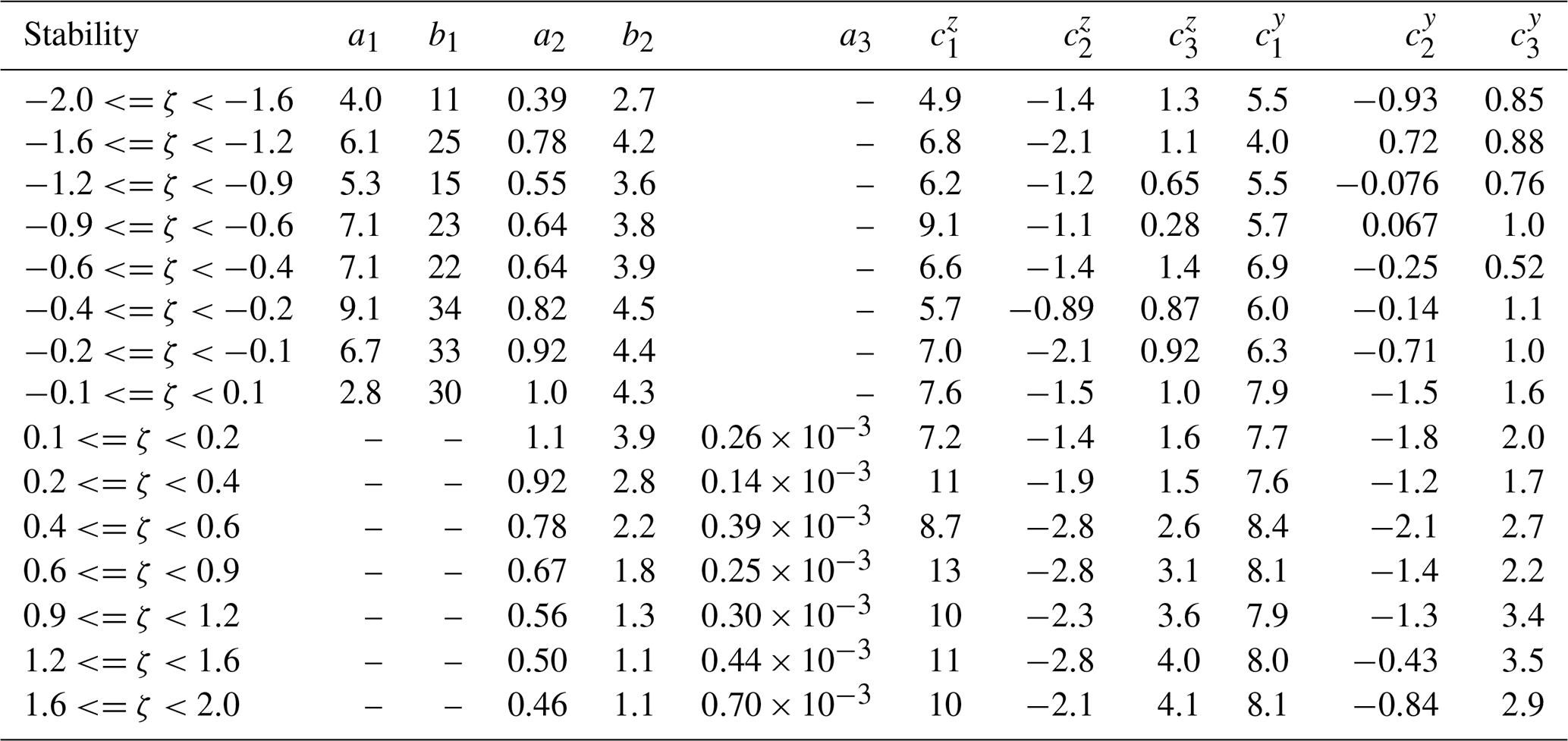
The empirical coefficients c₁, c₂, and c₃, estimated from the SRWS dataset, are shown in Fig. B1 and listed in Tables B1–B3.

Figure B1 Empirical model coefficients for computation of (a–c) vertical and (d–f) lateral coherence of the along-wind, cross-wind, and vertical velocity components. Values are obtained from least-square fits of Eq. (B1) to the SRWS measurements.

Table B1 Empirical model coefficients for computation of auto-spectra and coherence of the along-wind velocity component u. Values are obtained from least-square fits of Eqs. (A1)–(A2) to the sonic anemometer data at z=110 m and of Eq. (B1) to the SRWS measurements.

Table B2 Same as Table B1, but for the cross-wind velocity component v.

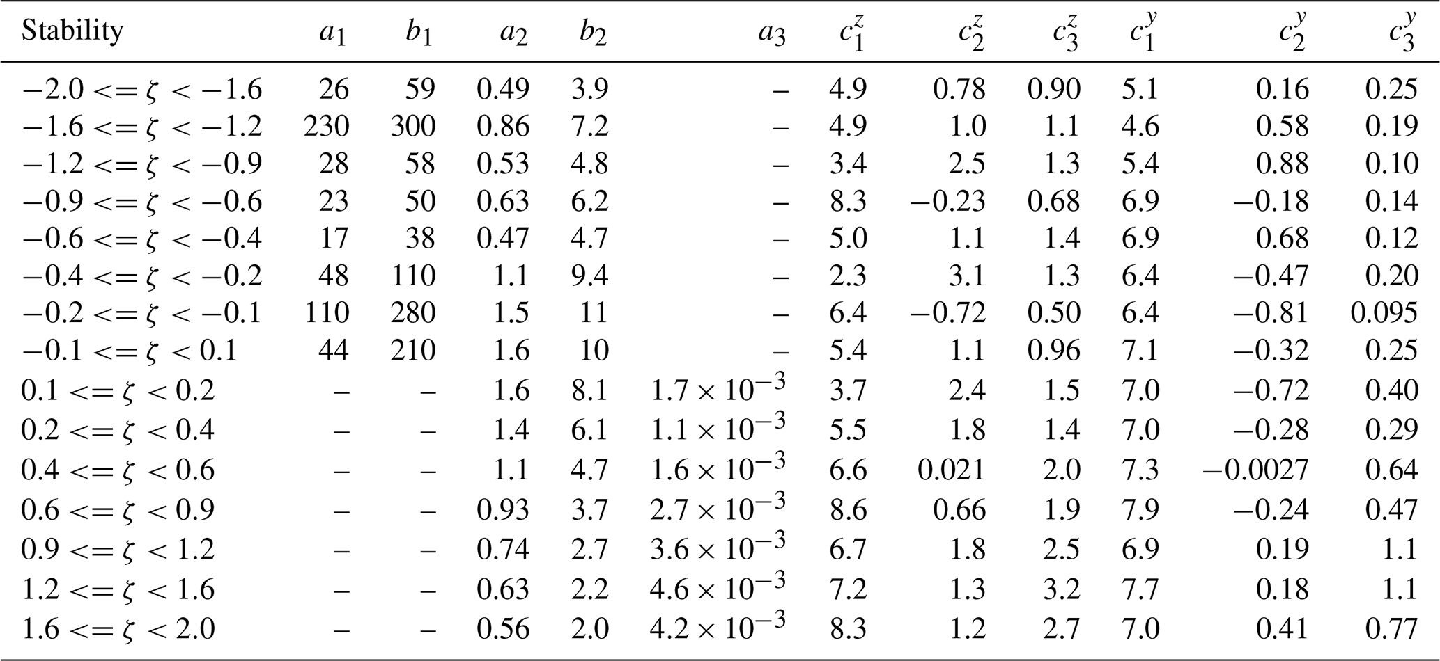
Table B3 Same as Table B1, but for the vertical velocity component w.

Appendix C: Atmospheric-stability distributions at z=55 m and z=25 m

Figures C1 and C2 present the occurrence of atmospheric-stability classes derived from the sonic anemometers at z=55 m and z=25 m, respectively. The distributions across mean wind speed, wind direction, month, and time of day exhibit trends similar to those observed at z=110 m (Fig. 8). However, the proportion of near-neutral conditions rises with decreasing measurement height, reflecting the increasing influence of mechanically generated turbulence near the surface. Consequently, neutral conditions account for more than 75 % of the observations for $U>\mathrm{13}\mathrm{m}{\mathrm{s}}^{-\mathrm{1}}$ at z=55 m and for $U>\mathrm{9}\mathrm{m}{\mathrm{s}}^{-\mathrm{1}}$ at z=25 m.

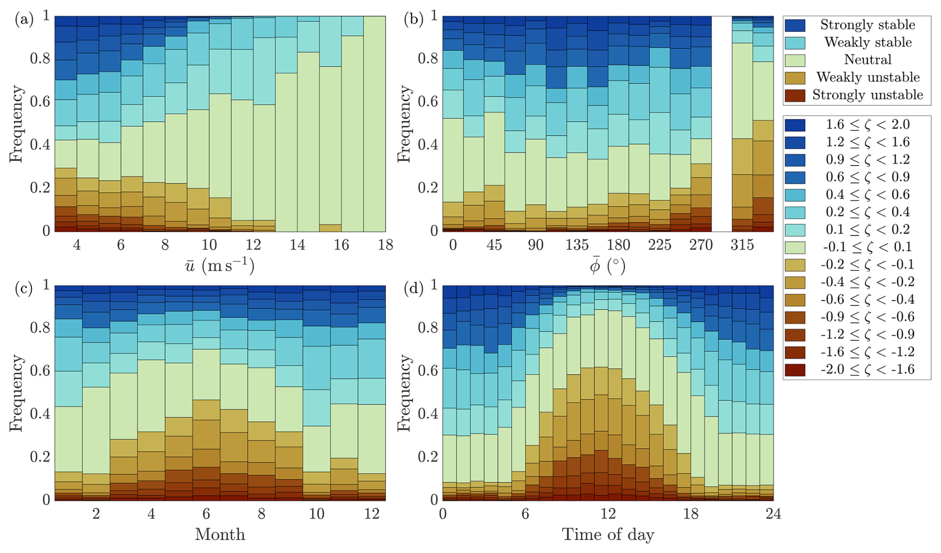
Figure C1 Occurrence of atmospheric-stability classes as a function of (a) mean wind speed, (b) mean wind direction, (c) month, and (d) time of day based on sonic anemometer measurements at z=55 m.

Figure C2 Occurrence of atmospheric-stability classes as a function of (a) mean wind speed, (b) mean wind direction, (c) month, and (d) time of day based on sonic anemometer measurements at z=25 m.