
the Creative Commons Attribution 4.0 License.
the Creative Commons Attribution 4.0 License.
 | 10 Nov 2026
Computational aerodynamics for leading-edge inflatable kite design
Jelle Agatho Wilhelm Poland

Kasper Raphaël G. Masure
Oriol Cayon
Roland Schmehl
Soft-wing kites are morphing, bridled, tensile lifting surfaces used for wind-assisted ship propulsion and airborne wind energy applications. Their swept-back planform, pronounced anhedral, and unconventional leading-edge geometry induce complex aerodynamic behaviour that challenges conventional modelling approaches. For leading-edge inflatable (LEI) kites, pressure-side separation induced by the inflated tubular leading edge renders classical inviscid methods insufficient, thereby necessitating sectional input from higher-fidelity approaches.
This study presents and applies a computationally efficient aerodynamic framework to an LEI kite by coupling a vortex step method (VSM) with RANS (Reynolds-averaged Navier–Stokes)-derived airfoil polars validated against wind tunnel measurements. The RANS simulations were used to train a machine learning surrogate model to facilitate parametric design studies. The application of machine learning to LEI kite aerodynamics is novel, and the surrogate model achieves R2> 0.98 across the considered parameter space.
Three-dimensional load predictions for the TU Delft V3 LEI kite were evaluated against wind tunnel data and reference three-dimensional RANS simulations. Within the operational incidence range °, the predicted lift and drag agree with measurements to within 9 % and 13 %, respectively. Across this range, the framework reproduces the measured aerodynamic trends more consistently than the reference 3D RANS results, while reducing the computational cost by several orders of magnitude.
A rigid-body stability analysis indicated static stability in roll, pitch, and yaw, as well as aerodynamic damping in all three axes within the quasi-steady model.
Parametric analyses revealed inherent trade-offs between aerodynamic efficiency and stability, motivating the adoption of multi-objective optimization strategies.
The validated framework provides high predictive accuracy at low computational cost and forms a foundation for rapid aerodynamic analysis, stability assessment, design optimization, and aero-structural coupling in the conceptual and preliminary design phases.
- Article
(9952 KB) - Full-text XML
- BibTeX
- EndNote


Soft-wing kites have expanded beyond their original use in marine sports to renewable energy applications, most notably airborne wind energy (AWE) and wind-assisted ship propulsion (WASP). A soft kite is a tensile structure consisting of a lightweight membrane wing supported by a bridle line system that transfers the aerodynamic loads and serves as the actuation mechanism (Oehler and Schmehl, 2019). These membrane wings fall into three types: ram-air wings, with two stacked membrane layers connected by membrane ribs and inflated by the incoming flow; leading-edge inflatable (LEI) wings, with a pre-inflated tubular frame supporting a single membrane layer; and single-skin wings, with a single membrane layer. Soft-wing kites are morphing aerodynamic control surfaces that deform through aeroelastic coupling (Breukels et al., 2013) and in response to actuation-induced changes in the bridle line system geometry (Hummel et al., 2019; Elfert et al., 2024).
Because the bridle line system transfers the distributed aerodynamic load of the membrane wing directly into tension, soft-wing kites achieve high lift-to-weight ratios in crosswind operation. For example, a 14 m2 LEI kite sustained a controlled tether force of 3 kN during crosswind figure-eight manoeuvres, corresponding to a load factor of approximately 20 relative to the 15 kg airborne system mass and 60 relative to the 5 kg wing alone (Van der Vlugt et al., 2019).
Design approaches common for sports kites rely heavily on experimental testing to determine the aerodynamic performance. Likewise, in AWE and WASP, control strategies rely on empirical measurements of control responses to inform gain tuning. When scaling kites to sizes required for commercially meaningful wind energy harvesting, such reliance on experiments becomes prohibitively costly, restricting iterative development cycles and increasing risks.
Instead, numerical simulation tools can be used effectively to assess kite designs, control responses, and stability derivatives, and to optimize flight paths in a virtual environment, without reliance on extensive prototype testing. To realize the full potential of these tools, fluid–structure interaction (FSI) phenomena must be accounted for by modelling the two-way coupling between aerodynamic loads and structural deformation (Candade et al., 2020). This FSI modelling has typically combined aerodynamic models with high-fidelity structural solvers through iterative coupling (Bosch et al., 2014; Lolies et al., 2019; Folkersma et al., 2020; Thedens, 2022). In these partitioned frameworks, the aerodynamic and structural solvers exchange loads and displacements in successive iterations until convergence. These iterative procedures make computational speed a critical factor, particularly in the context of design and optimization.
Simulating the aerodynamics of soft-wing kites is challenging owing to their complex geometry, which are characterized by a swept-back planform, low aspect ratio, and pronounced anhedral. A recent review synthesized the state of the art in AWE aerodynamics, spanning prototype architectures, and numerical and experimental methods from potential-flow models to high-fidelity Reynolds-averaged Navier–Stokes (RANS) and large-eddy simulation (LES) approaches (Castro-Fernández et al., 2026). Within this context, 3D RANS computational fluid dynamics (CFD) simulations of LEI kites have been conducted to explore variations in Reynolds number, angle of attack, and sideslip angle (Deaves, 2015; Viré et al., 2020, 2022). These studies, performed with k-ω shear stress transport (SST) turbulence and γ-Reθ transition models, revealed characteristic separation zones and 3D crossflow effects typical of curved, low-aspect-ratio wings. Despite providing valuable verification data, the high computational cost of these simulations makes them unsuitable for iterative optimization.
Lower-fidelity methods have been developed, including lifting-line (LL) and vortex-lattice formulations adapted for curved planforms and low aspect ratios (Gaunaa et al., 2011; Leloup et al., 2013; Branlard et al., 2022; Duport, 2018), as well as non-linear vortex-lattice and panel-based formulations capable of capturing moderate flow separation (Kappel, 2012; Leuthold, 2015). Panel and vortex-lattice methods fail for LEI kites because they cannot accurately capture flow separation and subsequent reattachment, which dominate the pressure side of the wing throughout most of its flight envelope (Folkersma et al., 2019).
A proposed multiple-wake extension (Leuthold, 2015) partially mitigates this limitation but ultimately suffers from the same underlying problem: when the reattachment line intersects a separation line, the model cannot robustly resolve the local flow topology. Accurately maintaining flow tangency and impermeability in these regions requires prohibitively fine body and wake discretization, leading to numerical instability and computational costs that undermine the method’s intended efficiency.
Taken together, these considerations motivate the use of LL-based formulations as a computationally efficient basis for aerodynamic simulation, as they retain the dominant 3D induction effects while avoiding the prohibitive cost of high-fidelity CFD.
The concept underlying these formulations dates back to Prandtl (1918), who modelled a finite wing as a bound vortex with a trailing vortex sheet and computed the sectional lift from the Kutta–Joukowski theorem (Kutta, 1902), evaluated with the vector sum of the freestream and wake-induced velocities. Two later developments are central to the present work. First, Pistolesi (1932) showed that the flow-tangency condition is best enforced at the three-quarter-chord point, an insight that Weissinger (1947) embedded in a discrete horseshoe-vortex formulation with improved robustness for swept wings (Dorn and DeYoung, 1947). Second, beginning with Tani (1934) and formalized by Piszkin and Levinsky (1976), the strict no-through-flow condition of classical potential-flow theory was replaced by a circulation-matching approach, in which the sectional circulation is iterated to consistency with prescribed 2D airfoil polars, yielding a hybrid viscous–inviscid formulation that admits non-linear sectional aerodynamics, including stall. Barnes (1997) combined both elements in the vortex step method (VSM), which Damiani et al. (2019) introduced to the AWE field, and Cayon et al. (2023) extended it to aero-structurally coupled kite simulations.
The predictive capability of any such formulation, however, hinges on implementation details and on the availability of representative airfoil polars for each spanwise wing section.
The present study focuses on kites with LEI wings, although the general modelling approach can be applied to other types of kite. For conventional airfoils, aerodynamic polars are commonly generated using tools such as XFOIL (Drela, 2013), which couples an inviscid panel method to an integral boundary layer formulation in a viscous–inviscid interaction framework. For LEI kites, however, the inflated leading-edge tube induces persistent pressure-side separation and recirculation across the full range of angles of attack (Folkersma, 2022), thereby violating the thin, predominantly attached boundary layer assumptions underlying such methods. Consequently, inviscid solvers are unlikely to be suitable for predicting the 2D flow around such geometries, requiring higher-fidelity viscous simulations, typically based on the RANS equations (Folkersma et al., 2019). However, this considerably increases computational demand, especially in the context of iterative aero-structural coupling, where the VSM discretizes the wing into multiple deforming spanwise sections, each requiring its own polar data.
To reduce computational effort, Breukels (2011) conducted 2D RANS CFD simulations for a parameterized family of LEI airfoils and derived a correlation model for airfoil polars. In this formulation, Cl is represented by a third-degree polynomial in the angle of attack α, whereas Cd and Cm are represented by second-degree polynomials. The polynomial coefficients are expressed as functions of the airfoil thickness ratio t and camber parameter κ, facilitating the efficient interpolation of aerodynamic polars within the considered range of airfoil geometries. While substantially reducing computational cost, the approach introduces several limitations, including discontinuities arising from empirical extrapolation beyond the simulated angle-of-attack range. Watchorn (2023) performed new 2D RANS CFD simulations and reported systematic deviations with Breukels for comparable airfoils.
A fast model alone is not sufficient; numerical models require rigorous validation to earn industry trust and deliver meaningful impact. Although 3D RANS CFD data can benchmark lower-fidelity methods in incidence and sideslip (Duport et al., 2019), wind tunnel testing is preferred. To remove structural and aeroelastic effects, a rigidized subscale model of the TU Delft LEI V3 kite was tested with a six-component load balance and stereoscopic particle image velocimetry to quantify forces and flow fields (Poland et al., 2026a, b). In a separate campaign on LEI airfoils, a stethoscope, infrared cameras, zigzag tape, pressure strips, and a pitot-tube rake were used to measure loads, assess forced transition, and characterize the flow (van Lith et al., 2026).
This study investigates the aerodynamic modelling of soft-wing kites using the V3 kite as the reference system, leveraging its openly available datasets and further establishing it as a community benchmark. The aerodynamic behaviour was simulated using an extended VSM. To provide reliable predictions at low computational cost, machine learning (ML) models were trained using 2D RANS CFD simulations. The substitution of potential-flow-based surrogate models with an RANS-trained ML model was evaluated against flat-plate data and 2D wind tunnel measurements (van Lith et al., 2026). The influence of the source of 2D input polars on 3D performance was assessed by comparison with wind tunnel experiments (Poland et al., 2026b) and 3D RANS CFD simulations (Viré et al., 2022). The study further examines VSM convergence characteristics, establishes recommended best practices, and derives rigid-body stability derivatives. Finally, kite design considerations are discussed by analysing the effects of variations in airfoil shape, planform configuration, and tow-point position.
The remainder of this paper is organized as follows. Section 2 describes the VSM, Sect. 3 introduces the 2D RANS CFD setup, and Sect. 4 introduces the deployed ML model generation and evaluation for 2D LEI airfoils. The results are discussed in Sect. 5, and design considerations are provided in Sect. 6.
The implemented VSM largely follows Cayon et al. (2023), which builds on the formulations of Ranneberg (2015), Damiani et al. (2019), and Jonkman (2021). The implemented method assumes steady flow around the lifting surface, such that the solution is restricted to the spatial domain and the starting vortex, presumed far downstream, can be neglected. For circulation matching, the flow is decomposed into a near-field region in the vicinity of each spanwise section and a surrounding far-field region dominated by 3D induction effects. The effect of the flow in the near-field region is characterized by non-linear viscous airfoil polars that govern sectional aerodynamic lift, drag, and moment, while the far-field flow induced by the bound and trailing vortices is treated as inviscid, incompressible, and irrotational within the vortex filament framework. These regions are coupled at a single spanwise location per section, namely the control point, where the Kutta–Joukowski theorem relates sectional circulation to the integrated lifting force. The VSM computes the aerodynamic properties of a given wing through a number of steps, illustrated in Fig. 1 and described in order in Sect. 2.1–2.5.
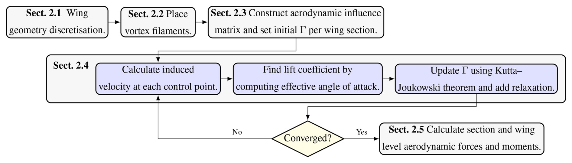
Figure 1Flowchart of the VSM, integrating the table-of-contents structure. The three stacked layers represent preprocessing (top layer), iterative circulation matching (middle layer, Sect. 2.4), and postprocessing (bottom layer). After geometry discretization and initialization, the spanwise circulation distribution Γ is solved iteratively until convergence, after which the sectional and global aerodynamic coefficients are evaluated.
2.1 Wing geometry discretization
To ensure methodological consistency, the geometry of the TU Delft V3 kite was adopted from previous CFD studies (Viré et al., 2020, 2022) and wind tunnel experiments with a rigid scale model (Poland et al., 2026a, b).
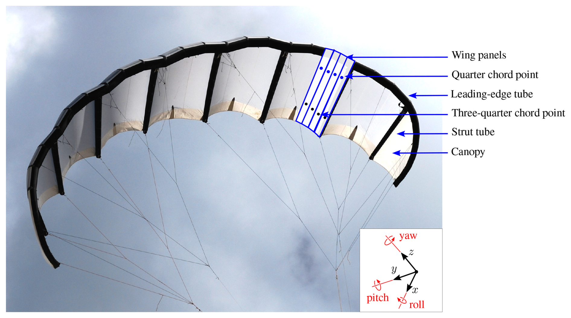
Figure 2Photograph of the TU Delft V3 kite taken in 2012, with wing panels superimposed for illustration purposes. The quarter-chord and three-quarter-chord points for each panel are indicated. The wing reference frame is defined with the x axis aligned with the mid-span chord line, the y axis oriented towards the left tip (when looking from the front) parallel to the LE tube at mid-span, and the z axis oriented in the direction of the bridle lines.
Representative airfoils were extracted as chordwise slices through the wing (see Fig. A1 in Appendix A). The discrete spanwise locations lie on the spanwise reference line defined by connecting the quarter-chord points, obtained at each station as
At each location, the section plane contains the global x direction and is oriented in such a way that its normal is perpendicular to the local surface normal at .
A formulation with planes aligned with the global x axis was selected rather than one oriented locally normal to the quarter-chord line. Although both formulations are equivalent in the linear lift regime, the latter introduces additional geometric non-linearities once Cl(α) departs from linear behaviour, which may bias the predicted load distribution (Fritz, 2024).
The wing is discretized into np panels, each constituting a fundamental element of the solver. The number of panels is not required to coincide with the number of chordwise slices used to define the geometry. For instance, when adopting a uniform panel distribution, both geometric properties (leading-edge (LE) and trailing-edge (TE) coordinates) and aerodynamic properties (2D polars) defined at the chordwise slices may be interpolated to an arbitrary value of np.
Because the panels are rectangular, they do not form a geometrically continuous surface representation. Instead, the panel system serves to define the bound and trailing vortex filaments, rather than to reproduce the exact wing geometry.
2.2 Vortex filament system
Following Kelvin’s circulation theorem and Helmholtz’s vortex theorems, all vortex elements must form a closed system; vortices cannot spontaneously appear or vanish within the fluid (Batchelor, 1967). Accordingly, the bound vortex filament, placed at the quarter-chord line of each panel, is connected to a trailing vortex filament that extends in the chordwise direction to the TE (see Fig. 3). At the TE, these are attached to wake filaments, which extend to infinity in the freestream direction u∞, in accordance with the frozen wake assumption (Ranneberg, 2015). Aligning the wake with the undisturbed free stream maintains consistency with the linearized LL formulation (Phillips and Snyder, 2000). Allowing the wake direction to depend on the locally induced velocity would introduce geometric non-linearity and require a free-wake treatment; and for strongly swept or highly anhedral configurations, spanwise-varying wake directions may additionally lead to filament convergence or intersection in a straight, semi-infinite filament model.
At infinity, the wake filaments are closed by an additional filament, thereby completing the vortex system. This closing filament is not explicitly modelled, as its aerodynamic influence at infinite distance is assumed to be negligible. The resulting vortex structure is known as a horseshoe vortex. Helmholtz’s theorems further require that the circulation strength remains constant along the length of each vortex filament (Batchelor, 1967); therefore, each panel has a single circulation value.
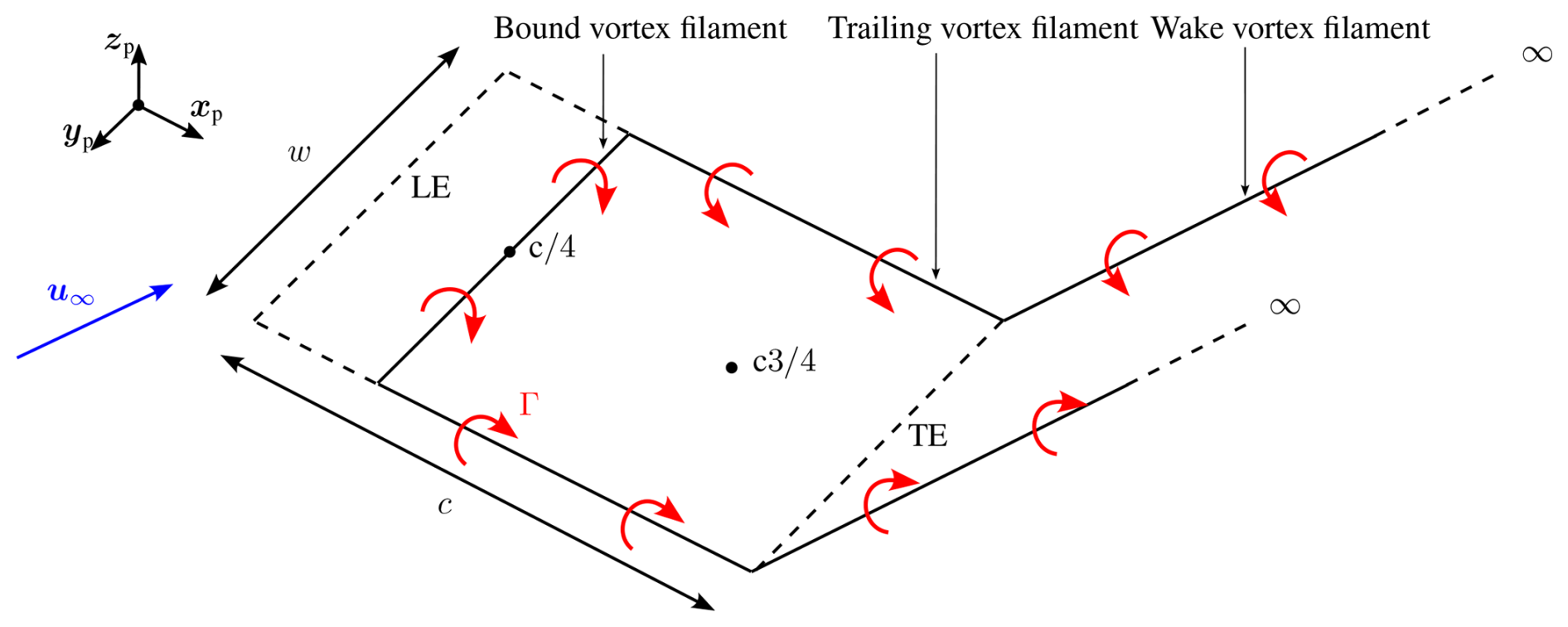
Figure 3Illustration of a single panel, showing the incoming freestream velocity u∞ in blue and the circulation Γ around each filament in red. The local panel reference frame – defined by the axes xp, yp, and zp – is indicated. The positions of the LE, TE, quarter-chord point , and three-quarter-chord point are also shown. Additionally, the panel chord c and panel width w are displayed.
The induced velocity vector uind at an evaluation point x due to a finite, 3D-bound vortex filament or chord-aligned trailing vortex filament is computed using the Biot–Savart law (Damiani et al., 2019):
where Γ is the circulation strength, r1 and r2 are vectors from the filament endpoints to x, and r0 is the vector along the filament segment.
For the wake filaments, which are modelled as semi-infinite vortex filaments, the induced velocity at x is given by Ranneberg (2015):
where r1 is the vector from the filament origin to the evaluation point, and is the wake-direction unit vector.
A vortex core model was employed to avoid singular behaviour by reducing the induced velocity at points located within a specified core radius, ϵ. For bound vortex filaments, the core radius is defined as a fixed fraction of the filament length; here, 5 % was adopted (Garrel, 2003; Damiani et al., 2019). For trailing and semi-infinite wake filaments, a viscous core model is adopted (Bhagwat and Leishman, 2002), with the core radius given by
where α0= 1.25643 is the Oseen parameter, ν the kinematic viscosity, and ℓ the relevant filament length.
For bound and finite trailing filaments, core regularization is applied for by evaluating the Biot–Savart velocity at the radially projected point xproj on the core boundary and scaling linearly:
The perpendicular distance to the filament centreline is
and xproj is constructed by keeping the axial projection of x onto the filament and setting its radial distance to ϵ.
For semi-infinite wake filaments, ϵ represents a viscous core of the far wake and is used only to desingularize the Biot–Savart kernel near the centreline. The corresponding perpendicular distance is
and for , the induced velocity is evaluated at the projected point xproj without additional scaling:
2.3 Aerodynamic influence coefficient matrix
To reduce computational cost during the circulation-matching iterations, the aerodynamic influence coefficients were precomputed once. Let denote the block aerodynamic influence coefficient (AIC) matrix that maps the spanwise circulation vector to the induced velocity at each control point. For panel , the induced velocity is given by
where denotes the (i,j) block of A and represents the induced velocity at control point i due to a unit circulation on panel j.
To ensure compatibility with non-linear airfoil polars, the near-field 2D self-induced contribution of panel i is subtracted at its own control point to avoid double-counting induction effects already embedded in the sectional polar data (Piszkin and Levinsky, 1976; Ranneberg, 2015; Damiani et al., 2019; Cayon et al., 2023). Define the per-unit-circulation 2D self-induced influence vector at control point i as
where is the local spanwise unit vector, and is the displacement from the bound-vortex centre of panel i to its control point. For a given circulation Γi, the corresponding 2D self-induced velocity is
The effective induced velocity used for circulation matching is then
This subtraction is applied only to the self-induced contribution of panel i and not to the cross-induced contributions from other panels.
2.4 Iterative solving for circulation
With the AIC matrix assembled, the spanwise circulation distribution was determined iteratively. At iteration k, the induced velocity vectors at all control points were computed collectively as
where vec(⋅) denotes the stacking of the three velocity components over all control points, and is the corresponding reshaped matrix whose ith row contains .
The effective relative velocity at the control point of panel i was then obtained by adding the local freestream velocity u∞,i to the induced velocity:
For each panel i, the sectional lift coefficient was obtained from the 2D polar using the effective angle of attack :
where , , and denote the local chordwise (LE-to-TE), spanwise, and panel-normal (upward) unit vectors, respectively.
The circulation at each panel was updated using the Kutta–Joukowski theorem, normalized by the local reference velocity magnitude:
where ci denotes the local chord length.
To ensure numerical stability, under-relaxation was applied globally to the circulation array:
The convergence metric δΓ was defined as the normalized maximum change in the global circulation distribution between successive iterations:
2.5 Converting to global properties
Once convergence was reached, the local aerodynamic force on each panel was computed as
where ρ is the fluid density, wi is the panel width, and Cl,i and Cd,i are the sectional lift and drag coefficients, respectively, evaluated at the three-quarter-chord control point. In other words, the local angle of attack evaluated at the three-quarter chord was used to obtain the aerodynamic coefficients from the 2D input data. The magnitude urel,i corresponds to the in-plane component of the relative velocity vector urel,i:
The force direction was set by an in-plane effective-flow direction following Ranneberg (2015), Jonkman (2021), and Damiani et al. (2019). This differs from the approach suggested by Li et al. (2022) and implemented by Cayon et al. (2023); the choice is motivated by comparing simulations of two geometries with wind tunnel measurements, detailed in Appendix B.
For each panel , the in-plane drag-direction unit vector is defined as
The lift was oriented in the normal direction , which was constructed as
The local aerodynamic moment on panel i was defined as
where Cm,i is the sectional moment coefficient; this moment represents the pitching moment about the quarter-chord point of the panel, consistent with the definition of Cm,i.
The contributions of all panels were summed and projected onto both the global coordinate directions , and , and the body-fixed aerodynamic directions: drag , aligned with u∞; lift , perpendicular to drag; and side , orthogonal to both drag and lift. With , the resulting non-dimensional force and moment coefficients are
where S is the projected planform area, cref the reference chord length, np the number of panels, the quarter-chord location about which the moment is defined for each panel, r0 the chosen global reference point, and the projection direction. The centre of pressure rcp was determined by
where F is the combined aerodynamic force vector of the wing, M0 is the combined moment vector about the reference point r0, and denotes the Euclidean norm of F. The resulting vector rcp lies along the line of action of the aerodynamic force and represents the unique point where this line intersects the wing surface. This intersection defines the effective location at which the resultant force can be considered to act, and it provides a critical indicator of aerodynamic stability, especially in relation to the trim state of the kite.
This section outlines the modelling framework used to generate aerodynamic airfoil data. It describes the profile parameterization, mesh generation, and simulation setup employed for the CFD analyses, followed by the convergence monitoring procedure.
3.1 Profile geometry parameterization
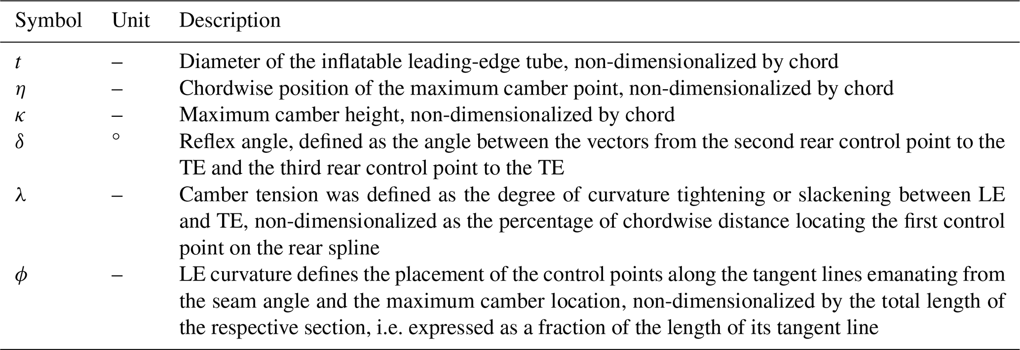
The parameterization presented here extends the earlier approach by Breukels (2011), who introduced two fundamental parameters: the circular LE tube diameter t and the camber height κ, shown in Fig. 4. Subsequently, informed by the experimental findings of Den Boer (1980), who observed a forward shift of the maximum camber position with increasing angle of attack, the chordwise location of maximum camber η was incorporated as an essential design parameter (Watchorn, 2023). Another step was to reduce the trailing-edge height from to zero, in accordance with the conventional airfoil definition (Kappel, 2012). A TE reflex angle δ is introduced, as this is often used to enhance the static pitching moment Cm and reduce the risk of front stall.
The LEI kite profile is constructed by defining a circular LE tube, smoothly extending it towards the maximum camber location using a Bézier curve named the front spline, and subsequently connecting it to the TE via another Bézier curve called the rear spline (see Fig. 4). Tangent continuity is enforced at both the junction between the curves and at the TE, ensuring aerodynamic smoothness. In this way, the profile shape can be characterized through six design parameters, summarized in Table 1.
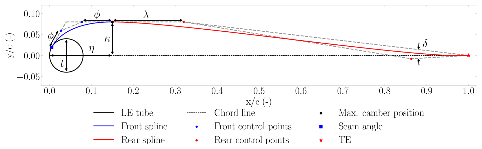
Table 1Overview of the profile shape parameters used in the Bézier-curve-based parameterization.
Each Bézier curve is defined by four control points [], with the parametric coordinate controlling the interpolation:
The front spline connects the seam to the maximum camber point. The seam, i.e. the stitched junction at which the canopy is attached to the LE tube, is located on the tube circumference at the seam angle. Because a tensioned membrane cannot sustain a bending moment, the canopy must depart the tube surface tangentially; tangent continuity is therefore enforced at the seam. The seam angle is determined by a dynamic search algorithm that increases the angle stepwise until the apex of the resulting front spline coincides with the prescribed maximum camber point, thereby selecting the smallest seam angle for which a tangent departure is compatible with the prescribed camber. This generalizes earlier fixed seam-angle definitions (Watchorn, 2023), which can produce invalid geometries for weakly cambered profiles. On the physical kite, the seam additionally acts as the roughness element that trips the boundary layer, supporting the fully turbulent modelling assumption discussed in Appendix C.
The intermediate control points of the front spline are positioned along the tangent lines emanating from the seam and the maximum camber point, with the LE curvature parameter ϕ specifying their relative distance along these tangents. In this way, ϕ shapes the curvature distribution: larger values concentrate curvature near the centre of the curve, whereas smaller values shift it towards the endpoints. As surface curvature sets the local pressure gradient, ϕ effectively redistributes the suction along the front spline. Within the physically consistent range, however, this redistribution only slightly alters the pressure distribution and has a negligible effect on the integral coefficients (Masure, 2025), as the dominant flow features of LEI airfoils (the suction peak on the LE tube and the pressure-side recirculation) are governed primarily by t, κ, and η. For this reason, ϕ is held fixed during dataset generation (Sect. 4).
The rear spline connects the maximum camber location to the TE. The intermediate control points are governed by the camber tension parameter λ, which adjusts profile smoothness, and by the TE reflex angle δ. To enhance model robustness and reduce the number of free parameters, the third control point is positioned at 20 % of the distance from the second rear control point to the TE, measured from the second rear control point.
3.2 Meshing
To ensure a smooth computational mesh, the LEI kite profile geometry requires specific adaptations. In particular, the sharp corner at the junction between the lower canopy and the LE tube is smoothed using a fillet. In addition, a canopy thickness tcanopy is introduced to represent a realistic finite thickness, to distinguish top from bottom airflow, and to enable a rounded TE. The optimal fillet size and tcanopy were determined through a sensitivity study. Masure (2025) evaluated seven leading-edge fillet sizes on two reference profiles, spanning enclosed cross-sectional areas of 0.13–45.52 cm2 (conventional) and 4.22–137.12 cm2 (highly cambered) for c= 1 m. The smallest numerically robust configurations, corresponding to enclosed areas of 0.98 and 4.22 cm2, informed a fixed fillet construction rule that scales with the tube diameter and seam angle, and is applied uniformly to all geometries in the dataset.
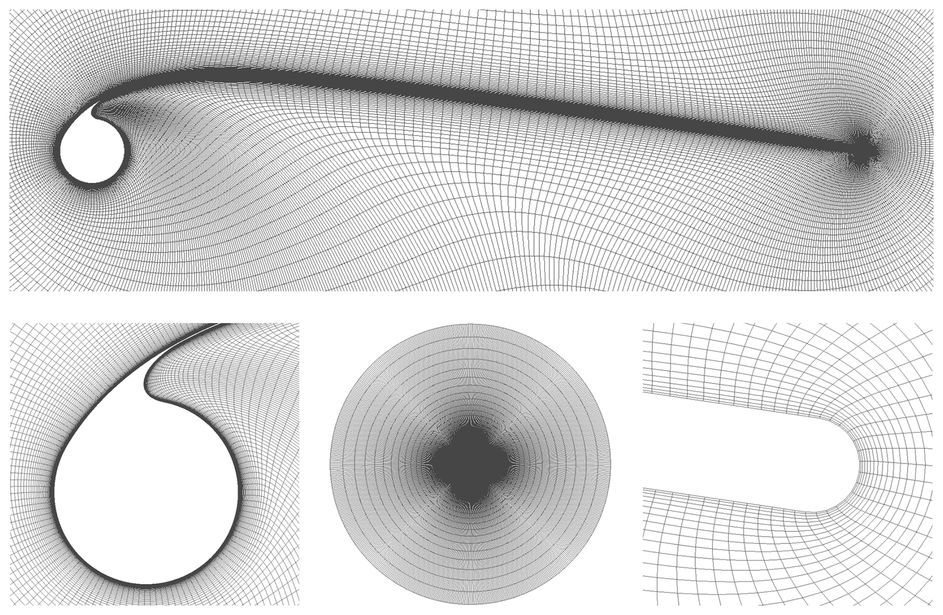
Figure 5Fully structured mesh (575 × 201) for an LEI kite profile with shape parameters t= 0.08, η= 0.15, κ= 0.08, δ= 0°, λ= 0.2, and ϕ= 0.65. The top panel shows the airfoil, and the lower panels depict, from left to right, the LE tube, the O-grid, and the TE.
A structured O-grid mesh with approximately 1.15 × 10⁵ cells, shown in Fig. 5, was generated for each profile using a hyperbolic-Laplace solver in Pointwise (Pointwise, 2025), automated via a Python script.
An O-grid topology was selected primarily for its insensitivity to angle-of-attack variations, which reduces the effort required for case setup, as only one mesh needs to be generated per profile. As the chord is normalized to unit length, the 2D mesh is extruded by a single cell over one chord length in the spanwise direction, as required by OpenFOAM's 3D formulation. In the wall-normal direction, the 201 cell layers are generated by hyperbolic extrusion with a fixed growth ratio of 1.1 following Watchorn (2023), starting from a first-layer height of 7.8 × 10⁻⁶ c, chosen to ensure 1 over the entire airfoil at Re = 5 ×10⁶. This places the circular far-field boundary at approximately 1.4 × 10⁴ chord lengths from the profile, sufficiently far for the freestream boundary conditions not to influence the computed force coefficients (Masure, 2025). Relative to the next-finer level, the selected production resolution of 575 × 201 cells changed the lift, drag, and moment coefficients by less than 2 % across the operational angles of attack, which is taken as the remaining discretization error.
For all cases, smoothing parameters for hyperbolic extrusion in Pointwise were applied uniformly to ensure mesh quality and numerical stability. The explicit smoothing parameter was set to 8 for transverse smoothing, while the implicit parameter was set to 16.0. Kinsey–Barth smoothing, with a value of 5, was used in the wall-normal direction to address regions of strong concavity. The volume smoothing parameter was set to its default value of 0.5.
Node spacing was uniform near the LE and TE, while a hyperbolic tangent distribution was applied along the canopy surface to minimize abrupt grid transitions. Mesh independence was assessed by Masure (2025), who independently varied the tangential (275–775 nodes) and wall-normal (161–221 layers) resolution of the structured O-grid for representative conventional and highly cambered profiles.
The non-dimensional wall distance y+ is defined as
where ρ∞ denotes freestream density, μ∞ the dynamic viscosity, and uτ the friction velocity.
3.3 Simulation setup
By assuming steady-state and incompressible flow, the steady RANS equations were solved using OpenFOAMv2006, with pressure-velocity coupling managed internally by the semi-implicit method for the pressure-linked equations (SIMPLE) algorithm (OpenFOAM, 2006). For an overview of the numerical schemes, the reader is referred to Masure (2025). The revised k-ω SST model by Menter (1994) was employed due to its robustness in capturing both near-wall and outer-region flow physics, supported by prior implementations in aerodynamic studies of LEI kites (Folkersma et al., 2019; Viré et al., 2020, 2022; Watchorn, 2023). All simulations were performed under the assumption of fully turbulent flow, owing to the measured turbulence intensities, the surface roughness present on both suction and pressure sides, and the high Reynolds numbers; a more elaborate discussion of this modelling choice is provided in Appendix C.
The inlet velocity scalar u∞, set to 1 m s−1, was projected in the direction of the angle of attack α to define the inlet velocity vector
The turbulent kinetic energy ki is defined as
where I represents the freestream turbulence intensity. The specific dissipation rate ωi at the inlet was defined as
where represents the eddy viscosity ratio. Values of I= 2 % and 10 were selected based on the sensitivity studies of Folkersma et al. (2019) and Viré et al. (2020).
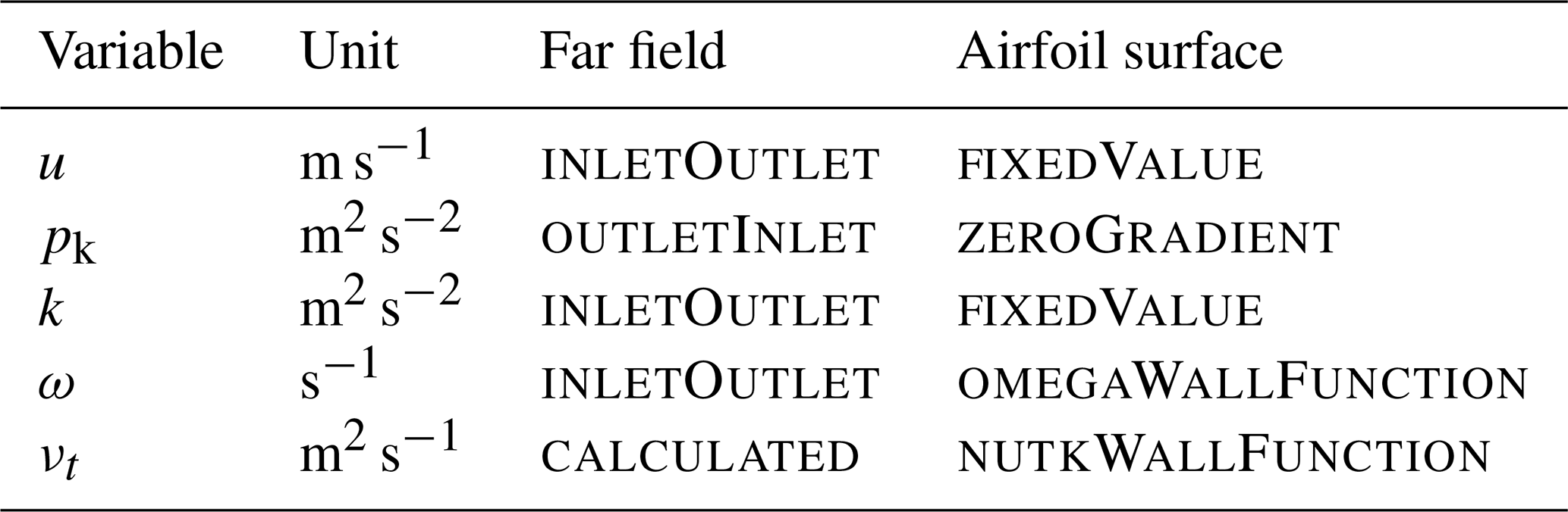
Boundary conditions for velocity u, kinematic pressure pk, turbulent kinetic energy k, specific dissipation rate ω, and eddy viscosity νt were applied as summarized in Table 2. Far-field boundaries employed non-reflecting types; the airfoil surface was defined as a stationary, impermeable no-slip wall with appropriate wall functions for turbulence; and spanwise boundaries were set to empty.
Table 2Boundary conditions and units for velocity, pressure, and turbulence variables.
3.4 Convergence monitoring
Convergence was monitored through both equation residuals and aerodynamic force coefficients. Specifically, residuals associated with momentum, pressure, and turbulence variables ux, uy, p, k, and ω were required to fall below 10−6 (Ferziger et al., 2020), while the force coefficients Cl, Cd, and Cm were expected to converge to within 10−4.
In OpenFOAM, each outer iteration reports two residuals per variable: the initial residual, evaluated on the newly assembled equation before the inner linear solve and thus measuring how well the previous iterate satisfies it; and the final residual, which only reflects the inner linear-solver settings. Outer-loop convergence is therefore monitored through the initial residual, on which the automatic stopping criterion acts. Because this criterion considers residuals only, a simulation could terminate before the force coefficients satisfy the 10−4 criterion. To prevent such early termination and ensure consistency across all cases, the stopping threshold was set slightly below the nominal residual criterion, at 8 × 10⁻⁷ for all flow variables. Each simulation was limited to a maximum of 5000 iterations. Cases not reaching the required thresholds within this limit were classified as non-converged; these typically occurred at high or negative angles of attack, where steady RANS solutions become unreliable owing to increased unsteadiness, e.g. flow separation.
For improved numerical stability, the velocity relaxation factor was set to 0.8, which dampened residual oscillations and improved convergence consistency. Representative histories for a typical LEI profile at α= 6° are shown in Fig. 6, where final flow residuals fell below 10−6 and force residuals just below 10−4.
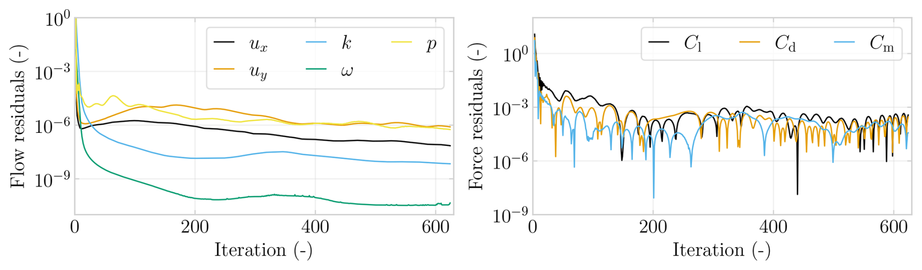
Figure 6Flow residuals at α= 6° for a profile with t= 0.0782, η= 0.178, κ= 0.0953, δ= 0.351, λ= 0, ϕ= 0.1.
This section presents the development and validation of a machine learning (ML) surrogate model trained on the aerodynamic database generated in Sect. 3. It describes the generation and filtering of the input data; the training and tuning of multiple regression algorithms; and the evaluation of their predictive accuracy for lift, drag, and moment coefficients.
4.1 Defining input profiles
Training data for the ML model were generated by varying the profile parameters, as shown in Table 3, over a range that encompasses physically viable profile designs. As varying ϕ within the marginal physically consistent range was found to have minimal aerodynamic influence, it was fixed at ϕ= 0.65, allowing greater resolution of the remaining parameters. The angle-of-attack range and sampling density were chosen to optimize accuracy in the lift polar and to maintain computational efficiency, with fewer points in the linear region (2° 10°) and negative α, and a finer step of 2° near stall. With ϕ held fixed, the sampled input space is six-dimensional (five varied-shape parameters and the angle of attack), analysed separately for three Reynolds numbers: Re = 1 × 10⁶, representative of small kites or static flight; Re = 5 × 10⁶, corresponding to typical in-flight operation; and Re = 2 × 10⁷, characteristic of larger kites and/or higher inflow velocities (Cayon et al., 2025; Masure, 2025).
Sampling Re at discrete levels is consistent with the fully turbulent modelling assumption (Appendix C). With transition fixed by the seam roughness elements and the elevated freestream turbulence encountered in operation, the regime changes associated with free transition are excluded. The force coefficients then vary weakly, smoothly, and monotonically with Re between the sampled levels, in line with turbulent skin-friction scaling, as quantified in Appendix D.
This is corroborated numerically by the 3D RANS results of Viré et al. (2022), which showed a negligible effect on the integral forces over a factor-two change in Re. It was also corroborated experimentally by the wind tunnel measurements presented in the companion paper (Poland et al., 2026b), in which the force coefficients varied only gradually and without abrupt regime changes across Reynolds numbers from 1.3 × 10⁵ to 6.1 × 10⁵. Only the lowest measured Reynolds number indicated an earlier stall onset, consistent with transitional effects at Reynolds numbers well below the fully turbulent regime considered here.
Table 3Design parameter ranges of the generated data for Re = 1 × 10⁶, 5 × 10⁶, and 2 × 10⁷.
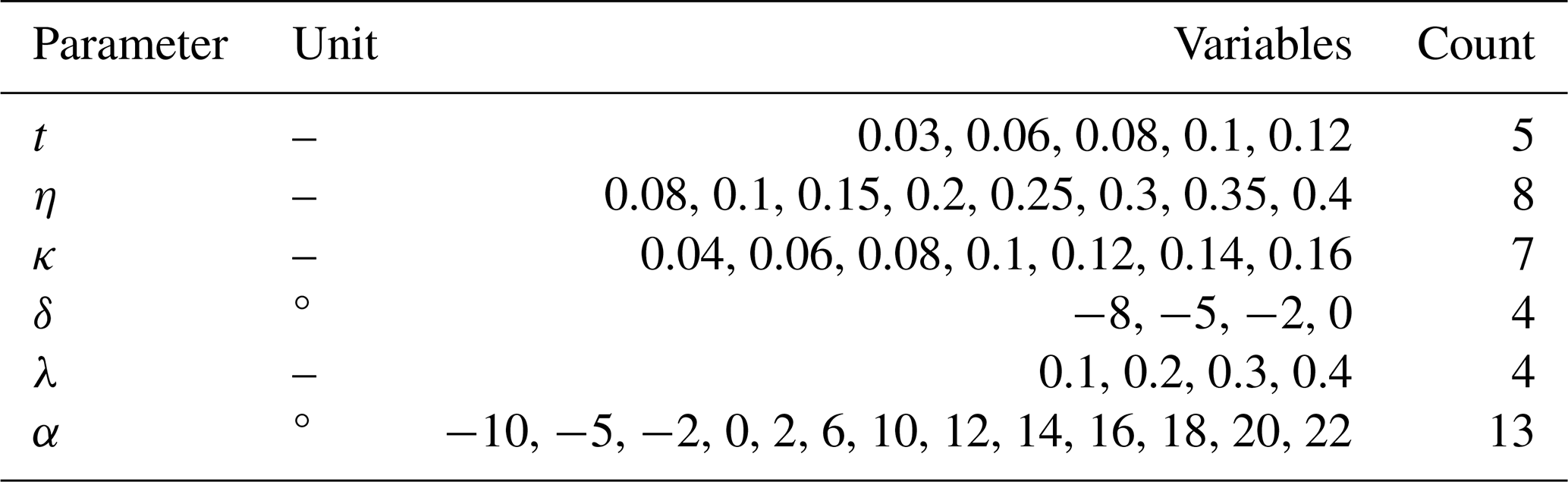
In preprocessing, the profiles were filtered out if the camber tension control point λ was positioned too far aft, i.e. 0.8, or if the camber height κ was excessively large, i.e. κ> 2.5t. After filtering, 3464 configurations remained per angle of attack, resulting in 45 032 simulations per Reynolds number.
4.2 Input data generation
Case generation was fully automated: for each profile-parameter combination in the design space, the scripts executed geometry construction, mesh generation, and case setup for the required angles of attack and Reynolds numbers without manual intervention. The resulting RANS CFD simulations were performed on the HPC-12 cluster at Delft University of Technology, with each case decomposed over four cores, requiring a total of 1.4 × 10⁵ core hours, corresponding to an average of approximately 1 core hour per simulation. A limited number of cases did not converge within 5000 iterations, predominantly at high angles of attack beyond stall, and were subsequently removed from the data.
Additionally, a z-score filtering approach (Dekking et al., 2005),
where μ represents the mean and σ the standard deviation, was used to identify and remove statistical outliers. Specifically, for each α and force coefficients, any data point with an absolute z score greater than 3 standard deviations from the mean was classified as an outlier and removed, illustrated in Fig. 7.
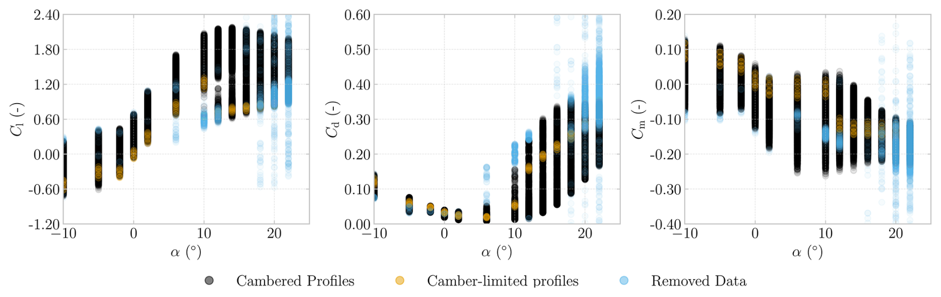
Figure 7Aerodynamic coefficients versus angle of attack for the Re = 5 × 10⁶ dataset, illustrating filtering of cambered profiles, camber-limited profiles, and removed data.
Profiles with a maximum camber smaller than tube radius, i.e. , are defined as camber-limited profiles and represent 0.23 % of the training dataset. For these cases, the number of parameters affecting the front and rear splines was reduced to t and δ, as the removed parameters had little to no effect. The camber-limited profiles exhibit distinct aerodynamic characteristics, producing lower lift and stalling earlier at approximately α= 10°. Consequently, they exhibit relatively high drag coefficients post-stall and increased pitching moments, indicating a stronger nose-up tendency in pre-stall flight conditions.
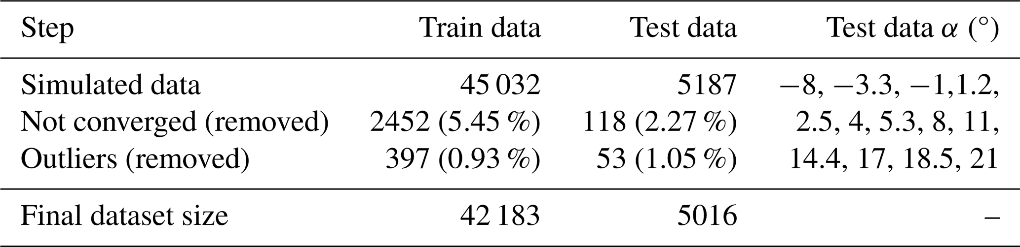
Building a predictive model within this design space requires the definition of both training and test datasets. A separate test dataset was constructed at different angles of attack from those used in the training set to verify the predictions at angles on which the model was not trained, shown in Table 4. After removing non-converged cases and statistical outliers, as summarized in Table 4, the final dataset comprises 42 183 training samples and 5016 test samples, corresponding to a test–train split of 10.6 %.
The test dataset exhibited a higher overall convergence rate, which was attributed to its narrower angle-of-attack bounds, making convergence less prone to failure near the limits, i.e. at negative α or under stall conditions.
Table 4Data filtering steps and resulting sizes for the Re = 5 × 10⁶ dataset.
4.3 Model setup
A separate ML model was trained for each Re to predict Cl, Cd, and Cm from any given set of the design parameters and the angle of attack, resulting in a model with a 7D input space (six shape parameters and α) and a 3D output space. Because α enters as a continuous input feature, the model can be evaluated at any requested angle of attack, not only at the values contained in the training data.
By contrast, Re was deliberately not included as a model input: with only three sampled levels, a tree-based regressor would represent the Re-dependence as piecewise-constant steps between the training values. Instead, a separate model was trained per Re, and for intermediate Reynolds numbers the sectional polars are obtained by interpolating between the bracketing models in log Re, which yields a smooth and monotonic Re-dependence. The resulting surrogate model is applicable within the trained range Re under the fully turbulent assumption (Appendix C); transitional flow at substantially lower chord-based Reynolds numbers falls outside its scope.
The quantities Cl, Cd, and Cm were selected for the output because they represent key aerodynamic metrics and allow for the determination of the chordwise centre of pressure xcp, which is a crucial stability indicator. The centre of pressure is determined through
which yielded values within 1 % of those obtained by pressure integration (Masure, 2025).
Model development began with standardizing the filtered training datasets, after which several regression algorithms were evaluated using their default settings (Pedregosa et al., 2011). The selected models were chosen for their strong baseline performance reported by Pandala (2021), and linear regression was included for reference. The full ML workflow is described in Appendix D and illustrated in Fig. D1.
After an initial model run with default settings, hyperparameters were systematically fine-tuned using grid-search cross-validation. In this context, validation refers to the internal process of developing the regression model across different hyperparameter combinations using subsets of the training data before evaluating the final model's performance on an independent test dataset. The coefficient of determination R2 (Dekking et al., 2005), defined as
was selected as the scoring metric, where yi denotes the true value for each data point, the corresponding model prediction, the mean value of the observed data, and n the number of points in the dataset. The hyperparameter search utilized a k-fold cross-validation approach, dividing the training set into k= 10 subsets or folds, with 90 % of the data used for training and 10 % for validation in each iteration. This was feasible because the dataset was sufficiently large to provide ample training data for improving model accuracy, measured here by R2, while still reserving a large enough test set to ensure reliability, as quantified by a low standard deviation.
Tree-based regressors yield piecewise-constant responses, so although the model returns a value for any requested α, the raw prediction varies in fine steps rather than continuously. Where a continuously differentiable polar is required, e.g. for derivative-based analyses or within iterative solvers, the model output is sampled at the training angles of attack. These samples are then fitted with a piecewise cubic Hermite interpolating polynomial (PCHIP) spline, whose shape-preserving, monotone formulation guarantees C1 continuity without introducing spurious oscillations. For a representative profile, raw predictions queried at arbitrary α deviate from the PCHIP-fitted polar by less than 0.03 in Cl (RMS 0.006), well below the regression error itself, confirming that the spline is a smoothness refinement rather than a required postprocessing step.
4.4 Model selection
After tuning was finalized, the performance of each model was assessed on the test dataset using three metrics: R2, the percentage root mean square error
and the percentage standard deviation
where n is the number of test samples, yi and are the true and predicted values, is the mean absolute value of the test targets, and ri and are the residuals and their mean, respectively.
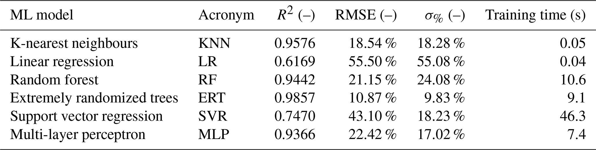
Table 5 shows the averaged results per model, from which extremely randomized trees (ERTs) were selected as they outperform the other algorithms, achieving the highest R2, and lowest RMSE% and σ%.
Table 5ML model verification using R2, RMSE %, and σ% for the Re = 5 × 10⁶ model.
4.5 Model evaluation
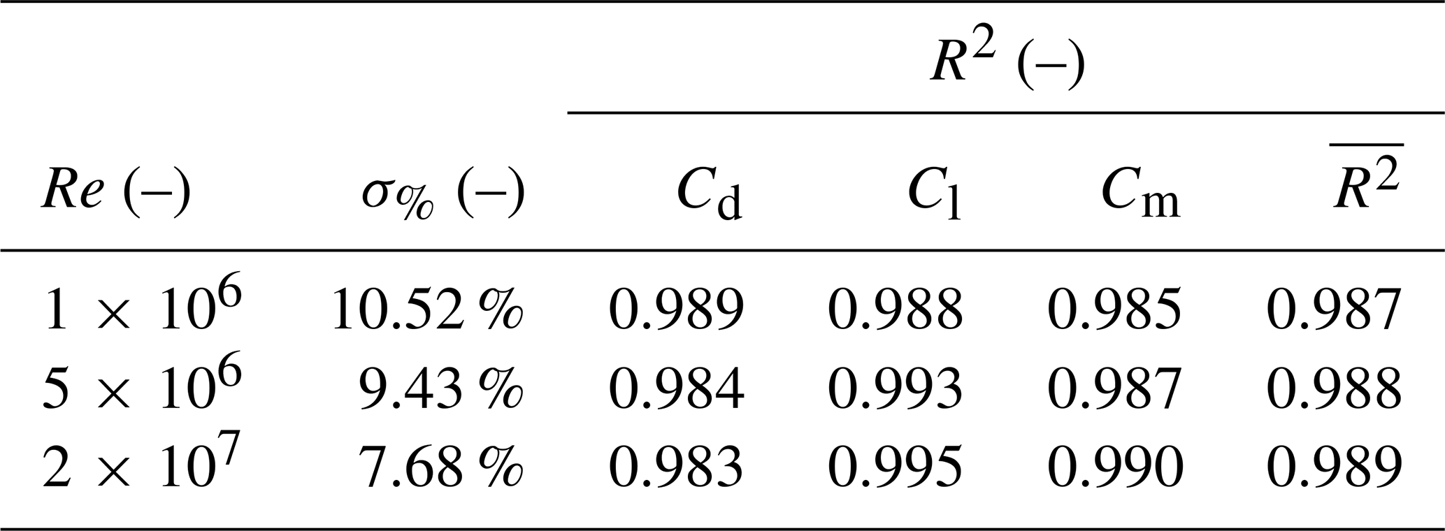
As shown in Table 6, the ERT exhibited high predictive accuracy with R2> 0.98 across all Re. The standard deviation σ% decreased with increasing Re, indicating greater prediction consistency and improved alignment with CFD predictions at higher Re.
To further evaluate the model's performance, three distinct and representative profiles were selected from the test dataset, detailed in Table 7. The third profile is notable as it represents a camber-limited configuration. The prediction metrics for these profiles are summarized in Table 7 and illustrated in Fig. 8 for Cl, Cd, and Cm.
In the plots, the ML model is evaluated at the angles of attack present in the training data, and the PCHIP spline introduced in Sect. 4.3 provides a C1-continuous polar through these predictions, from which the coefficients are interpolated at the test angles of attack for comparison with the true test data.
Overall, profile 2, with t= 0.086 close to the LE tube thickness of the mid-span profile of the V3 kite, exhibited the highest R2 values and the lowest RMSE% values, indicating the greatest predictive certainty. No consistent trend was observed in a specific force coefficient; for example, R2 and RMSE% were highest either for Cd or for Cm. In general, a lower R2 corresponded to a higher RMSE, with the RMSE% showing larger absolute changes when mispredictions occurred. For instance, in the drag polar of profile 2, two clear mispredictions increased the RMSE% by a factor of 2 compared with Cl, where only a single misprediction was present. The drag polars of profiles 1 and 3 revealed a similar pattern: in profile 1, one large misprediction resulted in an RMSE% approximately four times greater.

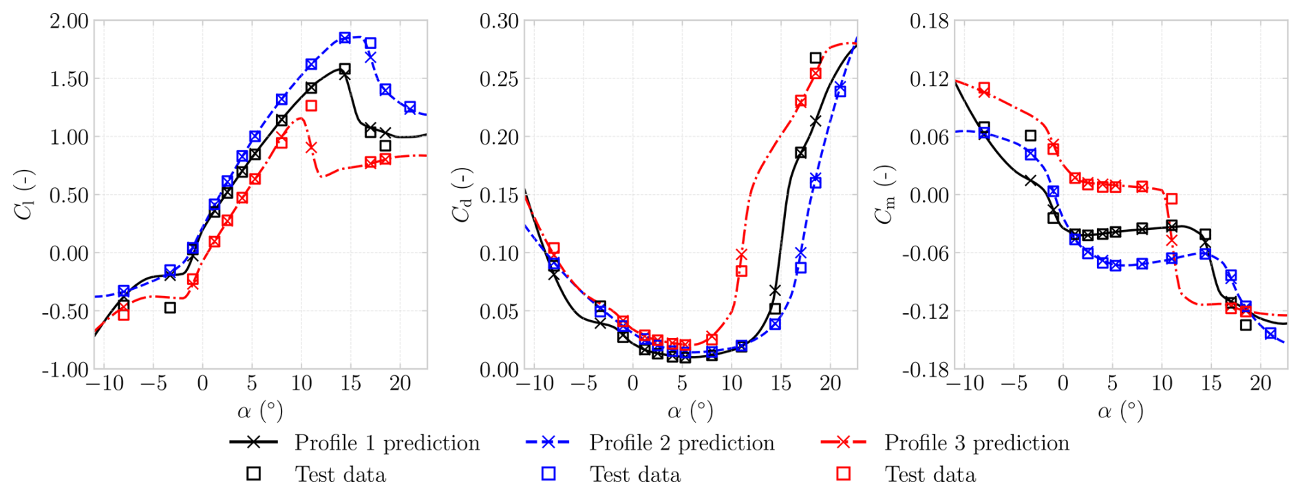
Figure 8Verification of the ML model using lift, drag, and moment polar for the Re = 5 × 10⁶ dataset.
This section reports the principal findings of the study, beginning with flow field observations and subsequently presenting a quantitative comparison of LEI airfoil polars. In addition, the VSM was examined with respect to its convergence characteristics and sensitivity to airfoil-level inputs; rigid-body stability derivatives were derived; and a concise synthesis of best practices and limitations was provided.
5.1 Flow field observations
The flow topology at α= 2° and α= 8° is shown in Fig. 9, indicating the pressure-coloured streamlines around the V3 kite mid-span airfoil and the corresponding surface distributions of Cp and Cf. From the pressure-side streamlines, it is evident that a recirculation region is present, splitting into two zones. The first is a corner eddy close to the tube; the second, larger zone is more sensitive to inflow angle variations, decreasing in size as α increases. The rotation direction of the pressure-side recirculation zone can be inferred from the friction coefficient; a negative friction coefficient indicates counterclockwise rotation.
At α= 8°, the Cp indicates a comparatively larger negative pressure peak at the suction side and shows a distinct upward pressure peak at the centre of the recirculation zone. Where the recirculation zone stretches to the airfoil's surface, the friction coefficient Cf displays a peak in the opposite (downwards) direction. Increasing α from 2 to 8° leads to a more concentrated and more negative peak. Furthermore, double values are plotted for both Cp and Cf in the region where, along a vertical line, one encounters three pressure-side surfaces, a distinct feature of an LEI airfoil.
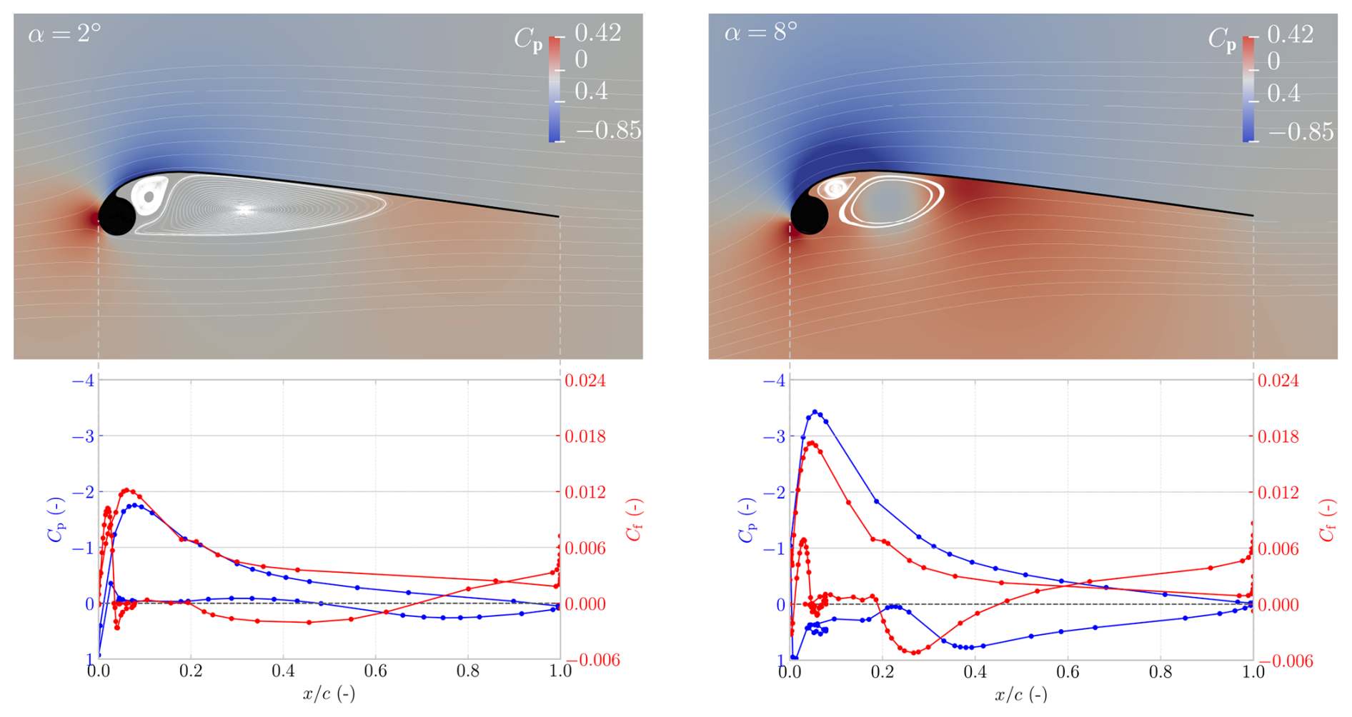
Figure 9Flow fields at α= 2° and α=8° for the V3 kite at Re = 1 × 10⁶. The figures present the surface pressure coefficient Cp and skin-friction coefficient Cf as functions of the non-dimensional chordwise coordinate .
5.2 Simulating airfoil aerodynamics
To assess the feasibility of inviscid methods for generating aerodynamic polars, NeuralFoil, a physics-informed surrogate model trained on tens of millions of XFOIL simulations and analytical solutions, was utilized (Drela, 2013; Sharpe, 2023, 2024).
Although XFOIL, on which NeuralFoil was trained, is not a purely inviscid method but a viscous–inviscid interaction solver, its integral boundary layer formulation assumes a thin shear layer coupled to an outer potential flow. Once separation becomes extensive and the flow no longer resembles a thin boundary layer attached to the surface, the mathematical foundation of the model is violated, and the predicted lift, drag, and pressure distributions can no longer be considered physically reliable (Drela, 2013). As LEI airfoils exhibit persistent pressure-side separation and recirculation that contravene these assumptions, the inclusion of NeuralFoil permits a structured assessment of the limitations of such viscous–inviscid approaches when applied to geometries dominated by extensive separated flow.
In this study, the largest model size, xxxlarge, was used; it achieves maximum errors of less than 0.3 % in the lift, drag, and moment coefficients relative to XFOIL (Sharpe, 2024). The boundary layer transition was set to 0 to mimic the fully turbulent assumption used in the deployed 2D RANS CFD simulations.
To put the LEI airfoil aerodynamic trends into perspective, the lift and drag wind tunnel measurements of a flat plate were used (Wick, 1954). Because moment measurements were not available, the moment polar was computed following classical flat-plate airfoil theory:
where α is in radians.
Figure 10 plots the lift, drag, and moment coefficients as a function of α for the mid-span airfoil of the V3 kite (shown in Appendix A), comparing classical flat-plate theory, flat-plate wind tunnel measurements, Breukels' regression model, NeuralFoil, 2D RANS CFD results, and wind tunnel measurements (van Lith et al., 2026).
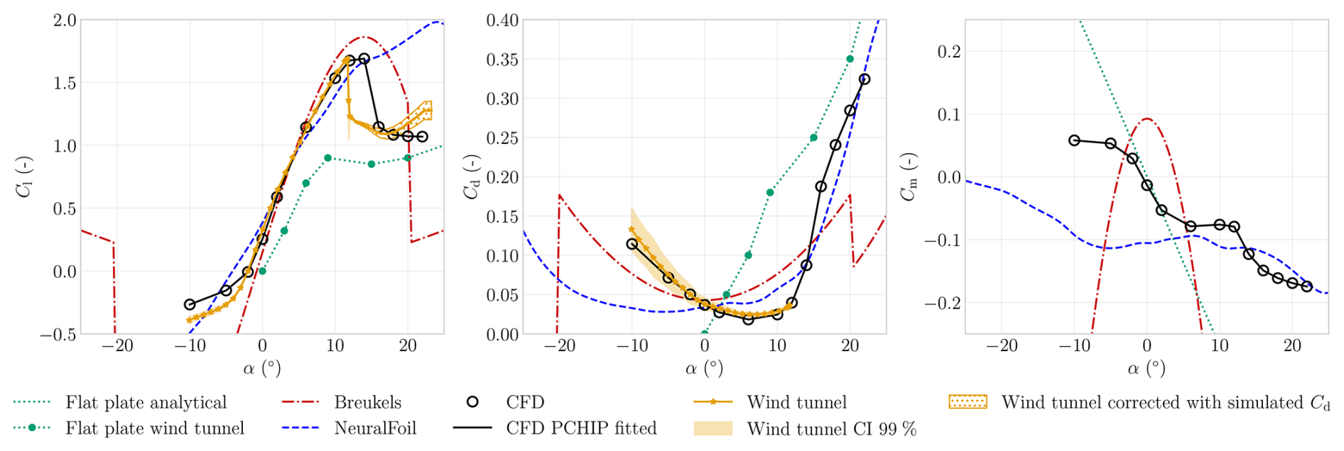
Figure 10The figure shows the airfoil Cl, Cd, and Cm as functions of α, obtained from different sources evaluated at Re =106. The NeuralFoil and CFD results use the ML profile-1 outline with minimal edge fillet, shown in Appendix A, to mimic the airfoil wind tunnel profile that had no edge fillet. The Breukels results used a larger edge fillet, corresponding to the CFD profile-1 outline in Appendix A. The numerical models, except for the flat-plate model, assume fully turbulent flow. This was mimicked in the wind tunnel measurements using zigzag strips, applied on the suction side at 3 % and on the pressure side at 45° of the tube, which were confirmed to be of sufficient height to induce transition (van Lith et al., 2026).
The predictions generated by Breukels’ regression model were considered invalid outside the range 20°. At these higher angles of attack, the extrapolated polars exhibited unphysical behaviour, including lift and drag discontinuities near 20° and negative drag coefficients for 20°, which were attributed to insufficient smoothing between the empirical expressions used to extrapolate the model beyond the CFD-simulated range. Furthermore, assuming symmetry and antisymmetry about α= 0° was considered inappropriate due to the airfoil's inherent geometric asymmetry.
In terms of lift, the NeuralFoil predictions align well with wind tunnel measurements and 2D CFD predictions up to approximately α= 13°. Beyond this range, however, NeuralFoil overpredicts lift and delays stall. For drag, between 5 and 10°, the NeuralFoil and Breukels' predictions exhibit similar trends to those of CFD simulations and wind tunnel measurements but are off in magnitude. At α> 20°, the Cd predictions of NeuralFoil and the CFD approach the flat-plate wind tunnel measurement in slope and magnitude.
Among all numerical approaches, 2D CFD simulations exhibit the closest agreement with wind tunnel measurements. Within the linear regime, from approximately 1° to α= 10°, the average percentage errors are 4 % and 16 % for lift and drag, respectively. The largest discrepancies occur outside the linear regime, in the negative-lift regime and in the prediction of the stall angle, where 2D CFD indicates a slightly delayed stall onset.
The largest discrepancies among the model predictions arise in the moment coefficient, for which wind tunnel measurements were unavailable for both the LEI airfoil and the flat plate. Breukels' model yields the greatest deviation from all other approaches. From 3 to 3° or so, the CFD results closely follow the flat-plate prediction for Cm. Beginning around α= 3°, the CFD-predicted Cm diverges from the flat-plate trend and instead flattens, maintaining an almost constant negative value from α= 5° to α= 12°. Beyond this point, a sharp decrease in Cm is observed, coinciding with the onset of stall. NeuralFoil is unable to capture this behaviour, and also deviates strongly with negative angles of attack.
5.3 VSM convergence
The VSM permits arbitrary spanwise panel distributions; for instance, the area between existing strut locations may be divided into equal parts, arranged with a uniform distribution or spaced according to a cosine-based scheme – commonly used in LL models to concentrate panels near the tips (Phillips and Snyder, 2000). However, for the V3 kite, the cosine distribution proved ineffective and failed to converge when the number of panels np exceeded 50, whereas a uniform panel distribution yielded the most robust and reliable convergence as np increased.
Within this paper, the simulations were considered converged when the metric δΓ< 1 × 10⁻⁶, and a relaxation factor of frelax= 0.01 was employed to ensure numerical stability.
Figure 11 demonstrates the convergence of aerodynamic coefficients by showing the percentage error relative to the np= 150 case for α= 2, 8, and 16°. The np= 150 case was selected as the endpoint because the VSM often failed to converge for larger values of np. The results were computed using airfoil data obtained from CFD simulations fitted with PCHIP, and the used V3 kite airfoils are shown in Fig. A2 in Appendix A.
The convergence analysis demonstrated that convergence deteriorated with increasing α, with markedly less smooth trends at α= 16°, consistent with VSM's post-stall behaviour, discussed in Sect. 5.4 and 5.6. Because the solution converged with increasing np, the largest panel count – np= 150 – was adopted throughout the remainder of the paper.
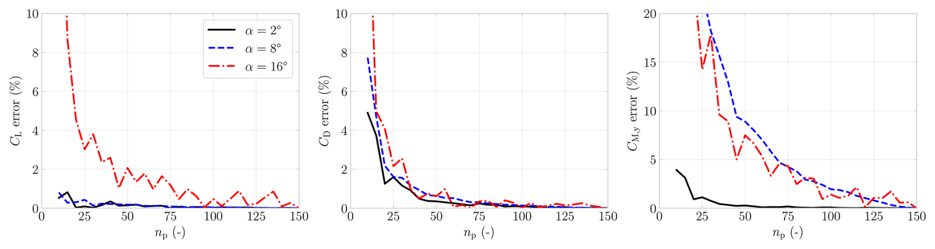
Figure 11Convergence analysis of the VSM for CL, CD, and CM,y at α= 2, 8, and 16°. The error relative to the reference case with np= 150 is shown.
5.4 VSM sensitivity to airfoil aerodynamic input
To place the VSM results with different airfoil inputs in context, wind tunnel measurements and accompanying confidence interval (CI) (Poland et al., 2026b) and 3D RANS CFD simulations (Viré et al., 2022) are plotted in Fig. 12, all at Re = 5 × 10⁵ except for the 3D CFD simulations, which are at Re = 1 × 10⁶. The 3D CFD simulations demonstrated that both the inclusion of struts and the difference in Reynolds number between Re = 1.0 × 10⁶ (with struts) and Re = 5.0 × 10⁵ (without struts) had a negligible effect on the integral forces (Viré et al., 2022). The plotted 3D CFD results differ from those presented in Viré et al. (2022), as they were corrected for a geometric offset of Δα= 1.02°; further details are provided in the appendix of the companion paper (Poland et al., 2026b).
The VSM results, generated with 2D RANS CFD PCHIP-fitted data, differ slightly from the geometry used in the wind tunnel and 3D CFD, as struts are omitted and differences between the profiles' pressure sides emerge near the tips, an artefact of relying on the parameterization scheme and an automatic meshing script (see Fig. A2 in Appendix A). The VSM results based on NeuralFoil, meanwhile, use the geometries with struts. The pitching moment CM,y was defined with respect to the tow point, defined as the location where the bridle lines converge beneath the wing, corresponding to the attachment point of the tether or kite control unit in AWE systems. The tow point of the V3 kite is located at x= 1.16 m, y= 0 m, and z= −11 m, relative to the mid-span LE point. The results are presented in Fig. 12.
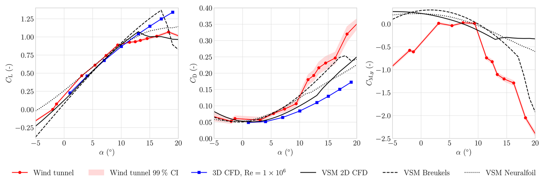
Figure 12The CL, CD, and CM,y are plotted over an α, for β= 0°, for varying VSM simulations, wind tunnel measurements, and CFD simulations (Viré et al., 2020; Poland et al., 2026b).
The V3 kite operates at α≈ 1° during reel-in and α≈ 8° during reel-out (Cayon et al., 2025), placing the nominal operating conditions largely within the near-linear portion of the polar. Accordingly, comparisons are assessed over ° to bracket the operational range and its associated variability.
Within this band, all results shown in Fig. 12 exhibited a consistent linear increase in lift, except for the wind tunnel measurements, which showed a change in slope at around α= 9°. At negative α, the VSM results based on 2D CFD data aligned most closely with the measurements. At higher α, where LL models are known to be inaccurate, the VSM 2D CFD predictions surprisingly agreed more closely with the measurements than the 3D CFD data. In drag, the sensitivity of the VSM predictions to the airfoil-level inputs was also evident: the VSM 2D CFD case – the only one without struts – yielded the lowest drag. Considering both lift and drag, the VSM with 2D CFD input reproduces the measurements more closely than the 3D CFD predictions. Averaged over °, the respective mean absolute errors are 9 % for lift and 13 % for drag.
The sensitivity of the VSM predictions is most evident in the pitching-moment coefficient CM,y, for which no 3D CFD data were available. The VSM results deviated from the measured trend at negative α and became less negative at higher angles. Within the mentioned α-band, all simulations predicted a continually decreasing CM,y, whereas the measurements showed a nearly constant and near-zero CM,y.
Overall, it is concluded that the VSM predicted the most consistent trends when using 2D CFD-derived aerodynamic input, primarily because the associated lift and drag polars capture stall behaviour more accurately.
5.5 Rigid-body stability derivatives
Rigid-body stability derivatives were obtained by perturbing the apparent velocity angles and the body rates about a trimmed baseline and evaluating the resulting changes in aerodynamic force and moment coefficients. Angle derivatives with respect to the angle of attack α and sideslip β were reported per radian, whereas rate derivatives with respect to the body rates p, q, and r (roll, pitch, and yaw) were non-dimensionalized to hat-rates using
where 2.346 m represents the mean aerodynamic chord with projected surface area S= 19.413 m2 and projected span b= 8.274 m. Sensitivity was then approximated using a central finite-difference scheme:
with perturbation steps 0.005 rad and 0.1 rad s−1. The reported derivatives were confirmed to lie close to the central-difference plateau: varying the angular step over 0.03–1.1° and the rate step over 0.005–0.1 rad s−1 altered every derivative by less than 0.3 % and 1 %, respectively, with the exception of the two yaw-moment derivatives and , which varied by up to 0.4 % and 3 %.
The perturbation steps were applied around the baseline trim angle, the angle at which 0 and 0, further discussed in Sect. 6. The trim angle was found at αtrim= 7.469°, with 2.708 rad−1, indicating local pitch stability. Moments were computed about the tow-point, i.e. the junction where the bridle lines connect beneath the wing, as this represents the physical point about which the kite rotates.
The resulting derivatives, reported in the aircraft reference frame in Table 8, represent instantaneous rigid-body stability characteristics; they do not capture unsteady aerodynamic effects or the influence of deformation on the dynamic response. As deformation was not included, control effects are likewise absent, because the kite wing relies on deformation for actuation. Despite this limitation, the aerodynamically derived stability derivatives still provide insight into the kite’s intrinsic stability characteristics, particularly given the scarcity of comparable data in the literature and the reference-model status of the V3 kite.
Table 8Computed rigid-body stability derivatives at the trim angle αtrim= 7.469°. All quantities are expressed in the aircraft reference frame, where the x axis is defined positive from the TE to the LE, the y axis is positive towards the right wing, and the z axis is positive downwards, forming a right-handed coordinate system consistent with standard aerodynamic force and moment sign conventions.
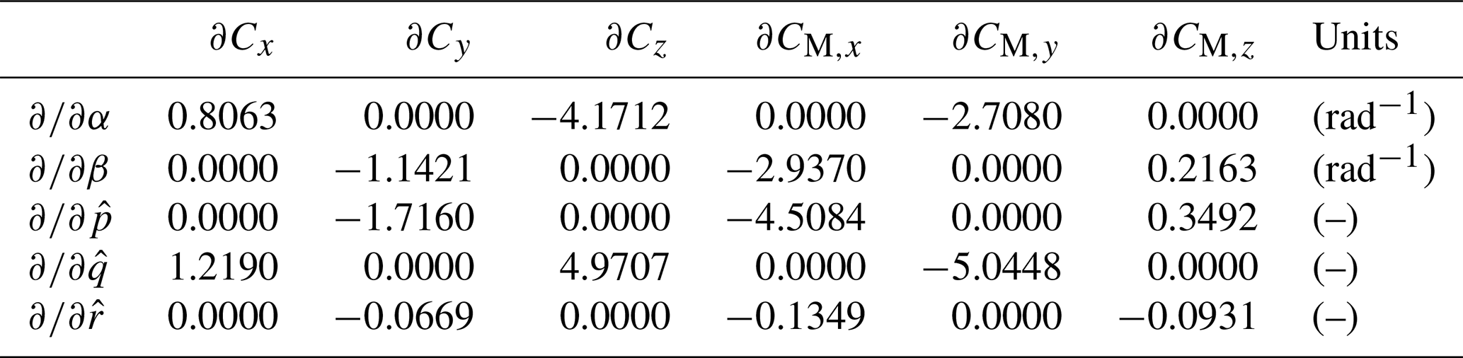
The signs of the static derivatives – , , and – indicated static stability in roll, pitch, and yaw, respectively (Etkin and Reid, 1996). The negative diagonal rate derivatives – , and – indicate aerodynamic damping in roll, pitch, and yaw, with yaw damping an order of magnitude weaker, consistent with the absence of a vertical stabilizing surface. Aerodynamic damping alone does not guarantee dynamic stability; resolving the dynamic modes requires a full modal analysis, including inertia and unsteady effects.
5.6 Best practices and limitations
VSM, like other LL methods, is sensitive to implementation details, and inconsistent force evaluation can lead to non-physical performance improvements when these models are embedded in optimization loops.
For this reason, the present work has prioritized internal consistency and documented limitations over incremental extensions whose theoretical implications are not fully validated.
Examples of excluded incremental extensions include accelerating convergence by initializing the solver with a previously converged circulation distribution. This strategy was omitted because the solution exhibited sensitivity to the initial condition, particularly in the vicinity of stall.
Extensions proposed for swept and sideslip configurations were explored but not adopted. The first concerned a sweep-consistent kinematic projection, in which the sectional kinematics were evaluated in the plane normal to the local spanwise direction when coupling the 3D induced velocity to 2D polars, rather than in the global projection plane used in the present VSM formulation; this modification produced only modest changes in the predicted loads. The second involved a modified near-wake treatment, in which the trailing vorticity was initialized locally perpendicular to the lifting line before aligning with the far-wake direction (Goates and Hunsaker, 2021), instead of being directly aligned with the free stream. This modification reduced the predicted lift of the V3 kite by nearly 40 % and was therefore not retained.
At high angles of attack, convergence issues may arise when the lift curve becomes non-bijective, such that multiple values of α correspond to the same Cl, particularly in post-stall regimes (Anderson et al., 1980; Chattot, 2004; Mukherjee and Gopalarathnam, 2006; Hunsaker, 2007; Gallay and Laurendeau, 2015; Dias, 2016; Simonet et al., 2024). Similar discontinuities were observed for the V3 kite in post-stall. To address potential spanwise discontinuities, a simple smoothing algorithm was implemented to damp sharp local gradients in the circulation field during iteration. However, no consistent results were obtained, as the smoothing effectiveness varied with both the number of panels and the geometry. It was therefore decided to omit the proposed algorithm. The model of Simonet et al. (2024) was also tested, but it likewise did not yield consistent results and was therefore excluded.
Discrepancies in drag, most pronounced when comparing numerical results to wind tunnel measurements (Poland et al., 2026b), may arise from several sources. One notable factor is the absence of a spanwise viscous drag contribution in the baseline model. A correction for this effect, proposed by Gaunaa et al. (2024), accounts for spanwise flow by decomposing the local velocity vector into spanwise and perpendicular components. The correction was omitted from the current VSM implementation due to its empirical nature and limited impact, as it increased drag by approximately 1 %.
To aid convergence, smooth sectional polars are recommended. Computational cost can be reduced by using fewer panels or by switching from the open-source Python version to the open-source Julia version, which is about 30 to 50 times faster, and runs in approximately 3 ms with 36 panels and in 25 ms with 150 panels on a 12th Gen Intel® Core™ i7-1265U CPU. The 3D RANS CFD simulations required 19 394 s of CPU time (Viré et al., 2022), indicating a speed-up on the order of 106, although the processor specifications for the 3D RANS CFD computations were not documented.
The aerodynamic design of kites presents distinct challenges relative to conventional aircraft, stemming fundamentally from their reliance on structural tension for flight integrity and from differences in the centre of rotation. Kites are uniquely susceptible to two contrasting stall phenomena: front stall, which generally occurs at low, negative angles of attack; and back stall, which manifests at high, positive angles of attack.
A front stall is often an irrecoverable failure mode. Once the kite initiates a nose-down motion, it is driven into negative angles of attack, where it produces minimal or negative lift. As the aerodynamic loading vanishes, line tension drops and the tensile structure collapses, reducing the kite to an uncontrollable mass of fabric.
In contrast, a back stall usually allows for recovery.
During the pitching-back motion, the kite typically retains part of its line tension and thus much of its shape. Control authority can often be restored by depowering, which effectively reduces the angle of attack and stops the stall. When the pitching-back motion is asymmetric, or when depowering is applied too late or insufficiently, the kite often rotates naturally in such a way that its heaviest component – the LE – moves downwards first. As the kite accelerates downwards, the magnitude of the apparent wind velocity increases, which reduces the effective angle of attack. Once the angle of attack re-enters the attached-flow regime, the separated shear layer can reattach, thereby restoring aerodynamic loading. The resulting renewed line tension re-establishes control authority before ground impact, often with sufficient time to steer the kite and keep it airborne.
In-flight, bridled soft-wing kites naturally align themselves until the net aerodynamic force and the tether attached to the tow point become parallel, at which point the moment arm vanishes and (Cayon et al., 2026). This equilibrium defines the trim angle of attack αt, which remains nearly constant because the tow point offers negligible rotational resistance. For a fixed bridle geometry, this equilibrium occurs at a single inflow angle, as corroborated experimentally for two kites, including the V3 kite (Cayon et al., 2025). The angle changes primarily during the transition phases, because powering and depowering alter the front–rear bridle length ratio, which shifts the effective tow-point location and thereby modifies the pitching-moment balance that sets αt.
For AWE systems, the design objective is to maximize the system's (Loyd, 1980) at the trim angle while maintaining sufficient stability margins to prevent front stall, which requires careful coordination between the wing's aerodynamic characteristics and the bridle configuration.
This section therefore presents parametric studies to investigate the effects of airfoil shape in Sect. 6.1, wing planform geometry in Sect. 6.2, and tow-point location in Sect. 6.3. Gravitational contributions are neglected in this analysis, which is considered a reasonable assumption given the low weight of soft kites relative to aerodynamic forces (Cayon et al., 2026, 2025). Although aero-structural coupling and unsteady effects are not included, the results provide valuable insight into aerodynamic trends and design trade-offs, and should be interpreted in the context of these limitations.
6.1 Effect of airfoil shape variation
To quantify the sensitivity of kite aerodynamic loads to airfoil geometry, the ML model was deployed to systematically vary the geometric parameters κ, η, t, δ, and λ. The resulting airfoil polars were subsequently used as input for the VSM to evaluate the kite aerodynamic loads. All the airfoil slices, shown in Appendix A, were uniformly varied by the same percentage relative to the V3 kite reference, while ensuring that all parameter values, shown in Table 3, remained within the bounds used for ML model training. As the V3 kite had a reflex angle of δ= 0°, percentage-based variation was not feasible; therefore, each profile was modified instead by an equal absolute value. The resulting variations are plotted in Fig. 13, with the exception of λ, which, within the parameter bounds used for training the ML model, had the least visible profile change.
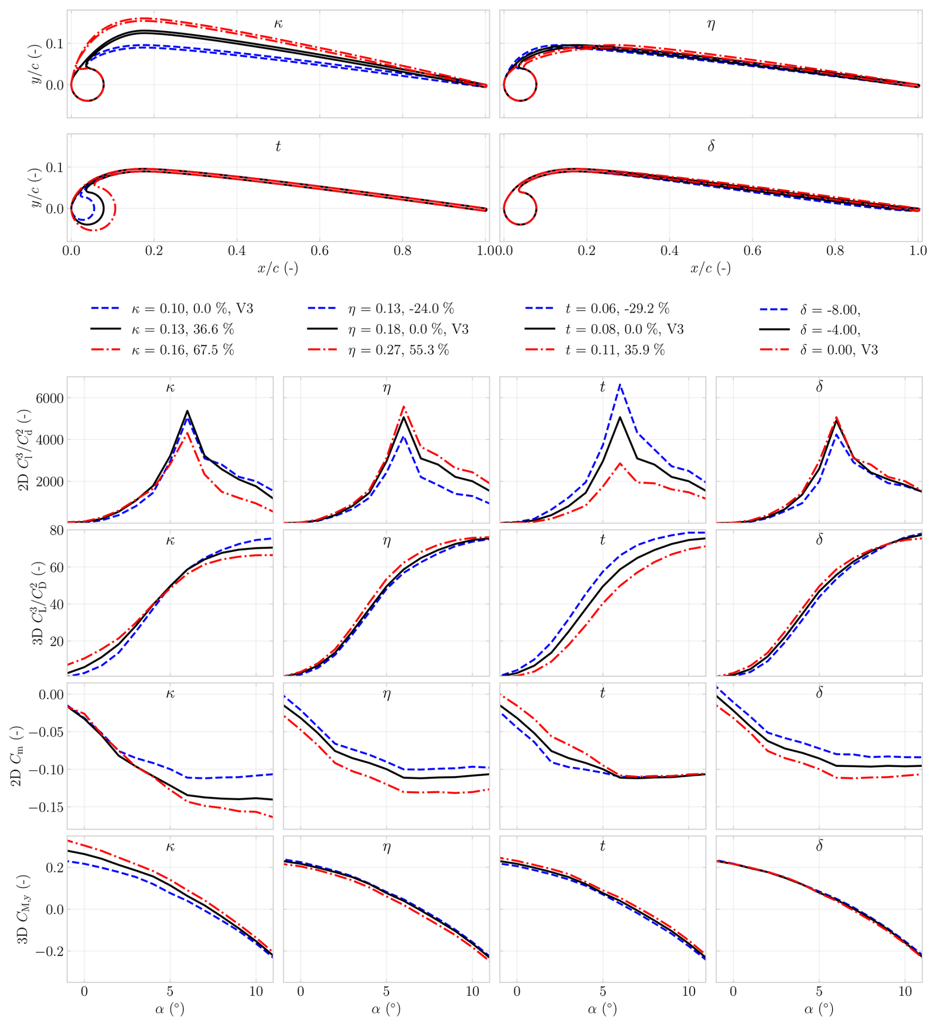
Figure 13Effect of changing the profile shape on the aerodynamic performance and pitching moment of the airfoil and wing.
The parameter study revealed that the effect on aerodynamic forces is more pronounced than the effect on the pitching moment. It furthermore showed that trends in 2D and 3D aerodynamic performance are not always aligned. For example, while the 2D ratio exhibits a clear peak near α= 6°, the gradually increases beyond this angle. Likewise, variations in t affected Cm differently depending on α; the 2D case exhibited a near constant trend at a 10° angle of attack, whereas the corresponding impact on the 3D CM showed a more uniform, decreasing trend across the investigated range.
For AWE, the aerodynamic design objective is to maximize the system ratio , evaluated at the corresponding trim angle. Compared to the V3 kite, the results indicate that an optimal design would have smaller values of κ, larger values of η, smaller values of t, and a small δ, although for the latter, the opposite holds for α> 8°.
6.2 Effect of planform variations
The effect of varying the wing planform geometry was analysed by simulating three distinct planforms. A cubic Bézier curve was fitted to the quarter-chord line of the V3 kite wing using four control points (P1, P2, P3, and P4) that preserved the endpoint positions at tip and root, as illustrated in Fig. 14. Two shape parameters, namely the distances from P1 to P2 and from P3 to P4, were employed to capture arc fullness and tip curvature. These distances were initially obtained by non-linear least-squares minimization of the total point-to-curve distance between measured quarter-chord points. The anhedral angle ϕan, also shown in Fig. 14, was defined as the angle between the line from P1 to P2 and the line from P1 to P4.
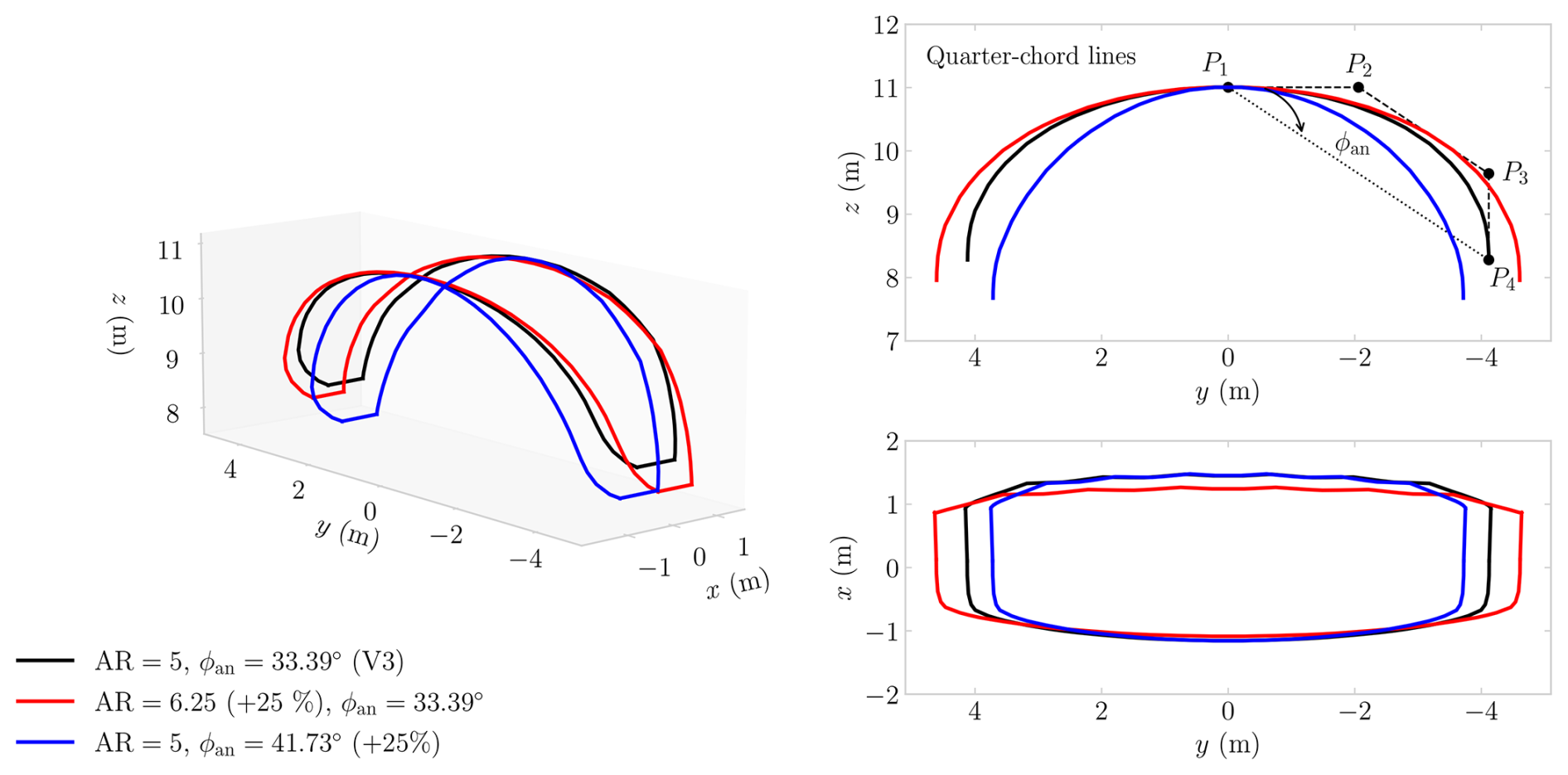
Figure 14Effect of changing the V3 kite's aspect ratio and ϕan, from its base properties, while maintaining the same flat surface area.
When reconstructing the V3 using cubic Bézier curves, an aspect ratio of AR= 5 was found, with AR defined as
where b= 11 m denotes the flat wingspan, not identical to the projected wingspan and measured as the quarter-chord arc length in the (y,z) plane when laid out flat.
A second planform with the same non-dimensional arc shape, but with a 25 % larger aspect ratio, was generated by keeping the shape parameters fixed, and scaling span and chord. A third planform was produced by increasing the anhedral angle by 25 % to ϕan= 41.73°. The flattened surface areas of the reference model and enlarged AR planform were nearly identical, where a reduction of less than 0.5 % was observed for the planform with enlarged ϕan.
The aerodynamic effects are presented for both α and β sweeps in Fig. 15. The trim angles, computed about the tow point, were αt= 6.89° for the baseline configuration, αt= 6.23° for the AR-scaled configuration, and αt= 7.20° for the ϕan-scaled configuration. As the maximum difference of 0.97° was not considered substantial in view of the applied shape changes, and to isolate the effect of the planform change, the β sweeps of all configurations were evaluated at the baseline trim angle of 6.89°.
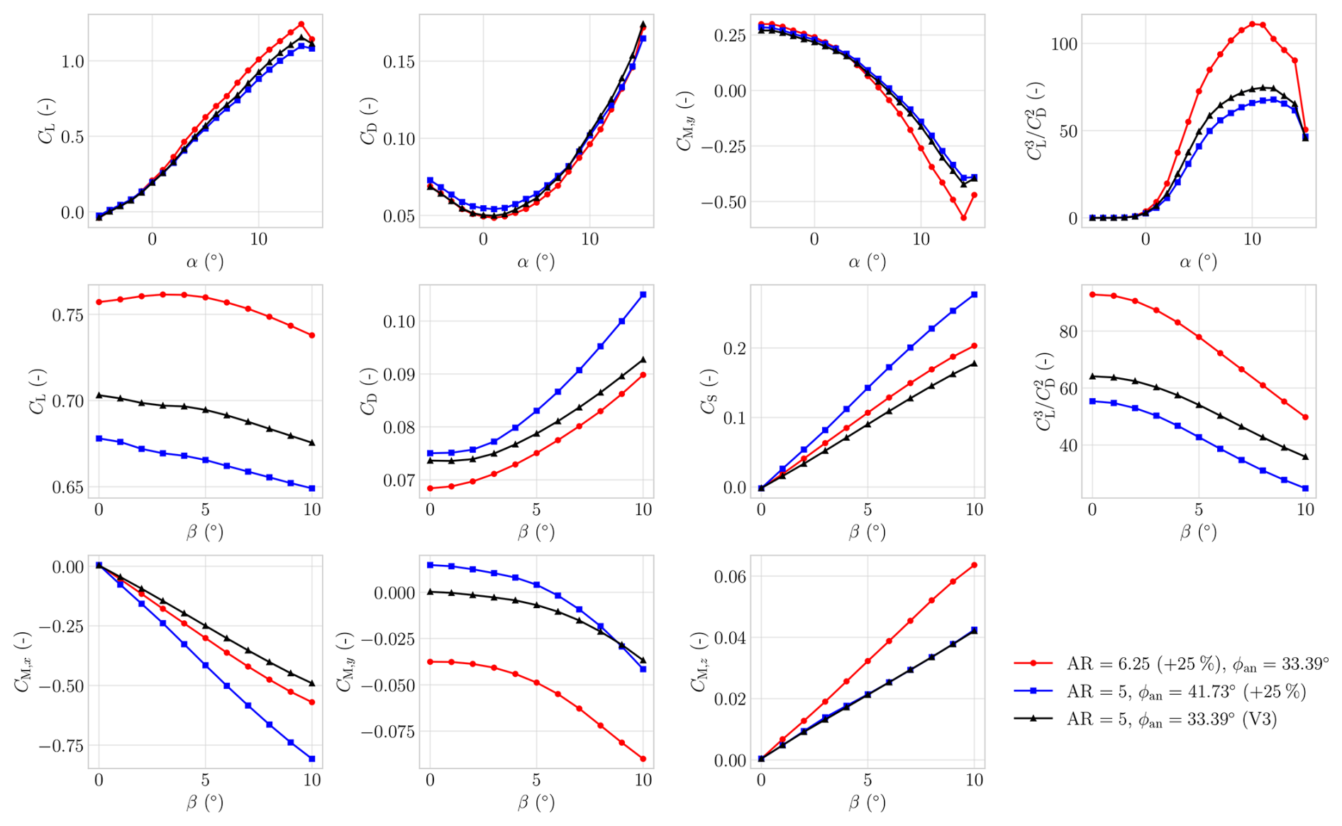
Figure 15Effect of changing the V3 kite, from its baseline, is shown by plotting the force and moment coefficients over an α and β sweep, the latter evaluated at the baseline trim angle αt= 6.89°.
Increasing the aspect ratio AR, in line with classical aircraft aerodynamic theory, resulted in higher values. This was accompanied by a more positive yaw-moment derivative . From this, one could conclude that a kite with a larger AR would generate a greater restoring yaw moment in response to an offset in β, thereby enhancing yaw static stability.
Increasing the anhedral angle ϕan reduced .
In addition, the lateral–directional coefficients exhibited stronger coupling: the side-force coefficient CS increased in magnitude for a given β, indicative of enhanced turning capability.
The results demonstrated a fundamental trade-off in kite design. Increasing AR yielded a higher lift-to-drag ratio, whereas increasing the ϕan lowered but enhanced the turning ability.
6.3 Effect of tow-point location
The sensitivity of the kite to variations in tow-point position was analysed by displacing its location in the x and z directions, as illustrated in Fig. 16, which also includes a V3 kite mid-span slice showing the LEI airfoil at the design distance, spanning precisely the figure x limits. For each tow-point configuration, the trim angle αt and its corresponding ratio were determined using the VSM. Since the VSM tends to lose accuracy in post-stall conditions, the analysis was restricted to the range .
The figures include a grey-shaded area indicating where , i.e. where the kite is not statically stable in pitch and no physically meaningful trim angle can be found. Additionally, the centre of gravity (CG) and the range of centre of pressure (CP) positions corresponding to the obtained trim angles were calculated and plotted.
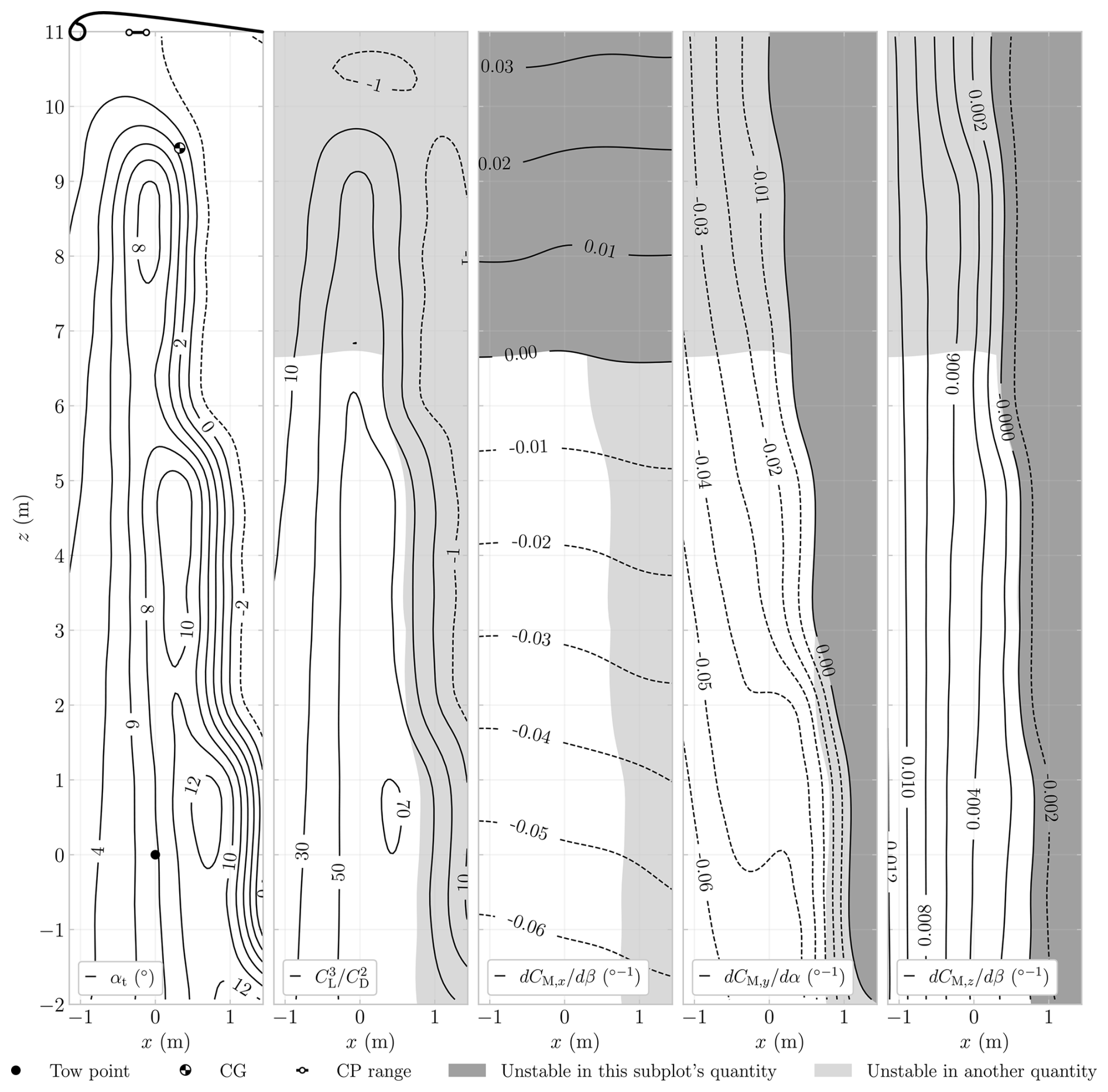
Figure 16Effect of tow-point displacement on the V3 kite aerodynamic characteristics. The left panel shows the mid-span airfoil, the CP range, and the CG. All plots show isolines of varying parameters. The left plot shows the trim angle αt as a function of tow-point location in the x and z directions. The other plots show the isolines for , , , and , with statically unstable regions marked by grey shading.
The results indicate that the trim angle αt is more sensitive to variations in x than in z. The same trend is observed for , , and . The largest trim angles αt, corresponding to the largest values of , occur when the tow point is positioned aft of the CP. However, positioning the tow point excessively close to the TE should be avoided, as it may lead to static pitch instability. More restrictive is the yawing-moment derivative , which shows that parts of the region yielding the highest coincide with , implying static instability in yaw.
The is the only parameter that is more sensitive to variations in z than in x, and it indicates static roll stability at the design tow-point location. The results show that raising the tow point can eliminate the restoring roll moment. This implies the existence of a boundary in tow-point height at which the effective roll moment arm about the wing changes sign, rendering the kite statically unstable in roll. As the CG lies above this boundary, placing the tow point at the CG location would lead to static roll instability. This behaviour is consistent with expectations for an anhedral wing in conventional aircraft (Etkin and Reid, 1996), and it underscores a key distinction: kites that rotate about a sufficiently low tow point require anhedral for roll stability, whereas aircraft that rotate about the CG require dihedral.
The tow-point variation analysis shows that to avoid static pitch and yaw instability, the tow point must be placed sufficiently far forward, which becomes more restrictive at higher z values. The stability gains of placing the tow point forward come at the cost of a reduced trim angle and, thereby, a lower aerodynamic performance.
A computationally efficient aerodynamic framework for soft-wing kite design was developed by coupling a vortex step method (VSM) with CFD-informed airfoil polars obtained from more than 105 RANS CFD simulations. The resulting novel RANS-trained machine learning (ML) surrogate model predicts lift, drag, and moment coefficients for parameterized LEI airfoils within the trained design space; three models were trained at Re = 1 × 10⁶, 5 × 10⁶, and 2 × 10⁷, achieving R2> 0.98 on held-out test data, with intermediate Reynolds numbers covered by interpolation in log Re.
Within the operational, near-linear incidence band °, selected to bracket the reported reel-in and reel-out angles of attack of the V3 kite, the underlying 2D CFD data agreed with wind tunnel measurements with mean errors of 4 % in lift and 16 % in drag. When these polars were used as VSM inputs, 3D lift and drag predictions matched wind tunnel results within this band on average by 9 % and 13 %, respectively, reproducing measured lift and drag trends more consistently than the available 3D RANS CFD results. The latter required 19 394 s of CPU time, whereas the present framework evaluated the np= 150 case in approximately 25 ms on the stated CPU, corresponding to an estimated speed-up of 𝒪(106) for the compared configurations, subject to differences in hardware, parallelization, and included preprocessing. This computational efficiency facilitates optimization, aero-structural coupling, and real-time control applications.
Rigid-body analysis yielded a novel, numerically derived set of static and rate (damping) stability derivatives for the TU Delft V3 reference kite. The configuration was found to be statically stable in roll, pitch, and yaw for the examined trim condition, and the computed rate derivatives indicate aerodynamic damping within the present quasi-steady aerodynamic model. A dedicated modal analysis, including unsteady aerodynamics, is required to characterize the associated dynamic modes.
Parametric analysis revealed that configurations maximizing aerodynamic efficiency, expressed as , do not coincide with those improving static stability margins (e.g. via and ), indicating a multi-objective design problem. Within the present quasi-steady, rigid-geometry analysis, the roll-stability mechanism reverses: anhedral is stabilizing for kites rotating around the tow point, whereas dihedral is stabilizing for aircraft rotating about the centre of gravity.
The framework provides a validated and computationally efficient basis for conceptual and preliminary kite design. Future work should integrate aero-structural coupling to resolve wing deformation and its feedback on aerodynamic loading, for example, by updating spanwise sectional polars in response to the local deformed airfoil geometry and operating point. In addition, optimization studies would benefit from incorporating variations in bridle geometry and tow-point positioning to quantify their coupled influence on aerodynamic performance and stability.
Geometric differences exist between the various simulation approaches. To illustrate these differences, Fig. A1 shows a spanwise slice taken at 25 % of the chord length of the V3 kite at α= 6°, plotted for half of the span.
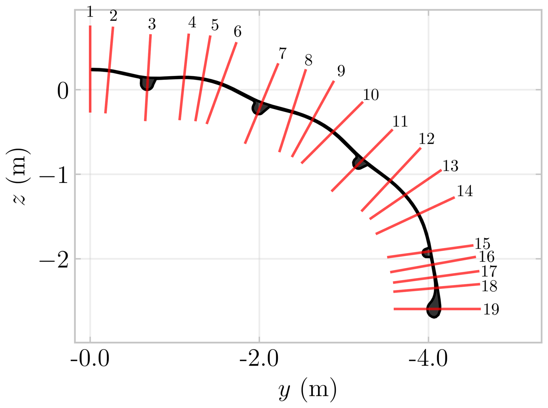
Figure A1Slice distribution along a representative spanwise section of the V3 kite at α= 6°, evaluated at 25 % chord. The figure is selected for illustrative purposes and does not correspond to the exact physical position.
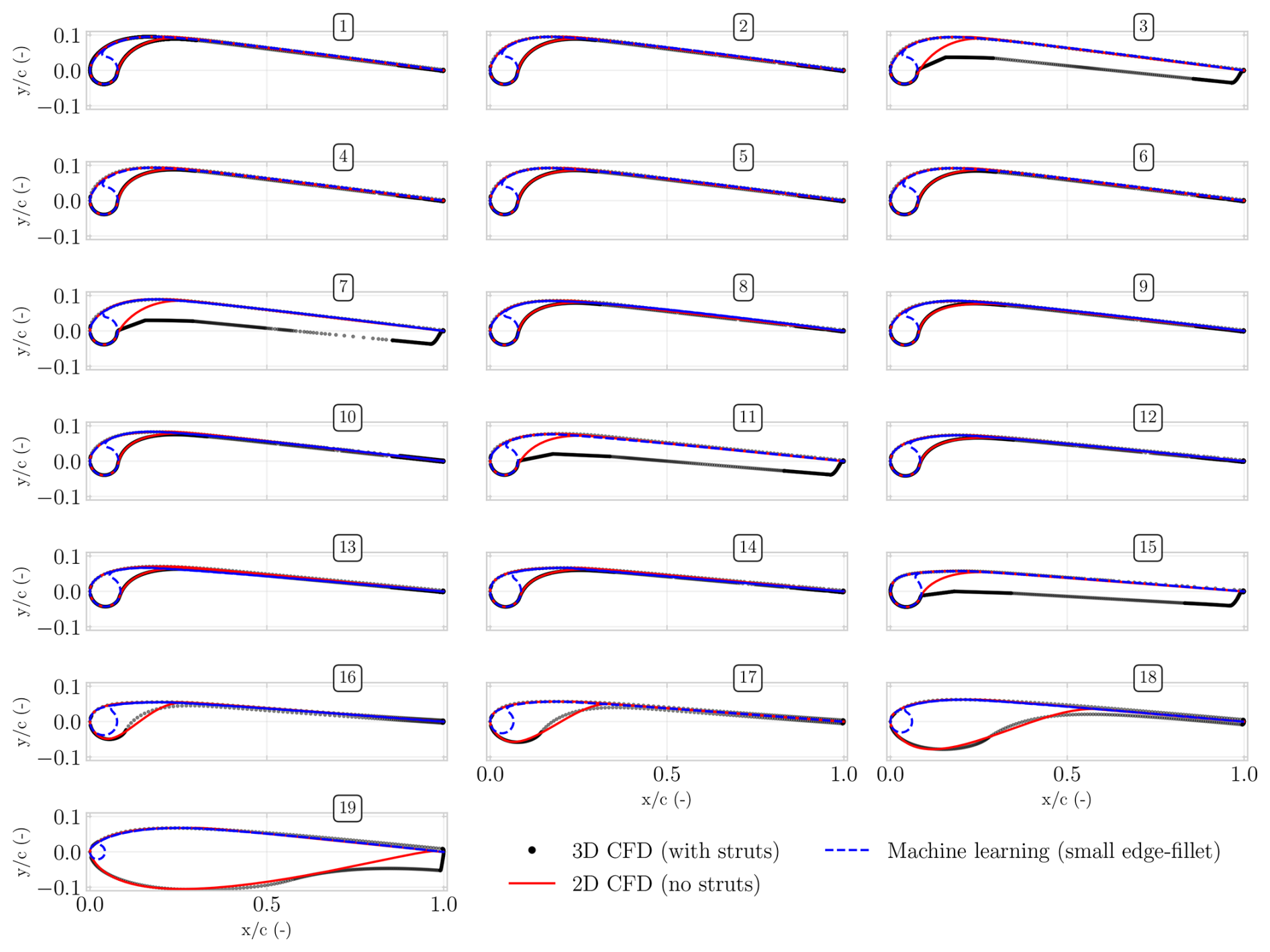
Figure A2Profiles used for simulations and their differences. A 2D CFD was also run on the dashed blue airfoil of profile 1 to better match the profile used in the 2D wind tunnel study, which had no edge fillet (van Lith et al., 2026).
As shown in Fig. A2, a total of 19 chordwise slices are defined, ranging from “1” at the mid-span to “19” at the tip. The three simulation techniques differ in the airfoil geometry across these profiles, illustrated in Fig. A2.
The 3D RANS CFD analysis conducted by Viré et al. (2020) employed a smoothed geometry, which incorporated substantial edge fillets downstream of the LE. The 2D RANS CFD simulations, undertaken to facilitate direct comparison with the 3D RANS CFD results, similarly included large edge fillets but did not account for the struts. The ML model, by comparison, was trained on 2D CFD datasets generated from geometries designed to approximate the physical configuration as closely as possible. Consequently, it cannot predict geometries with such large edge fillets; hence, only fillets of significantly reduced dimension are present relative to the other simulated geometries.
As the tip region was approached, the 2D slice intersected the LE tube at an increasingly shallow angle; that is, less perpendicular and more parallel to the tube axis. This progression increased the disparity between the respective geometries, most apparent for profiles 18 and 19 in Fig. A2. As the trained ML model focuses on the LEI airfoil shape, it does not capture these changes.
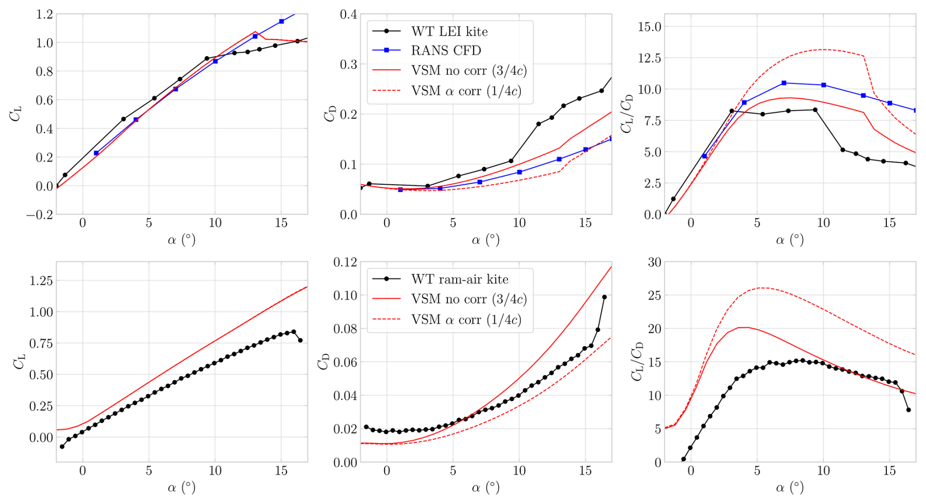
Figure B1Effect of varying the force-direction evaluation point, shown using VSM simulations performed at the Reynolds numbers of their respective wind tunnel (WT) measurements, which are included for comparison. Plotted are CL, CD, and against α for the TU Delft V3 LEI kite and the ram-air kite (Poland et al., 2026b; Belloc, 2015).
Li et al. (2022) revisited the chordwise placement of the control point in LL-type formulations by embedding unsteady 2D thin airfoil theory into a generalized 3D framework. Building on the classical thin airfoil solution, they showed that the quasi-steady lift magnitude is formally linked to the effective angle of attack evaluated at the three-quarter-chord point, consistent with the Kutta condition and with the location where the no-through-flow boundary condition is enforced in Weissinger-type discretizations. In contrast, the direction of the aerodynamic force is governed by the local flow angle at the quarter-chord point, where the bound vortex resides.
Li et al. (2022) validated their correction against blade-resolved RANS CFD simulations of wind turbine rotors with finite thickness and viscous effects, and demonstrated improved agreement for coned configurations. For a 15° coned rotor, the theoretically consistent two-point approach reduced power prediction errors by 8 %–10 % relative to simplified one-point implementations, resulting in noticeably closer agreement with CFD.
To assess the applicability of the correction, derived from unsteady thin airfoil theory, to highly swept, anhedral kite wings, VSM simulations were performed for the TU Delft V3 LEI kite and a ram-air kite using two alternative implementations: (i) a standard three-quarter-chord evaluation for both force magnitude and direction (), and (ii) Li's suggested approach in which the magnitude is evaluated at three-quarter-chord while the direction is evaluated at quarter-chord (). The validation dataset comprised wind tunnel measurements for both geometries, supplemented by 3D RANS CFD for the V3 LEI kite.
Figure B1 shows that, although both implementations predict CL accurately and are in close agreement with the measurements and CFD, the method systematically underpredicts CD relative to the reference data. As a result, the predicted is consistently overestimated. Both kites exhibit similar trends, with the discrepancy being most pronounced for the V3 LEI kite. In contrast to the wind turbine results of Li et al. (2022), the standard implementation yields better overall agreement with the experimental and numerical reference data, particularly for the key metric .
The reason why the correction degrades, rather than improves, the drag prediction accuracy is not yet understood. Consequently, it cannot be concluded that the method proposed by Li et al. (2022) is fundamentally incorrect. Instead, based on the present validation results, it is inferred that, for the investigated geometries, the standard implementation provides the closest agreement with the measurements and is therefore adopted throughout this work.
Li et al. (2022) additionally proposed a single-evaluation-point pitch-rate correction for unsteady cases. However, evaluating this correction requires validation data with known pitch histories, which are currently unavailable for these configurations; the present comparison is therefore limited to steady conditions.
In 2019, Folkersma et al. (2019) showed with 2D RANS CFD that explicitly modelling boundary layer transition affected the aerodynamic predictions for Re < 2 × 10⁷ under a low freestream turbulence intensity of approximately 2 %. This finding motivated the subsequent use of natural-transition models in 3D RANS CFD studies of the V3 kite (Viré et al., 2020, 2022). Recent field measurements of the Kitepower B.V. V9 kite system, however, reported turbulence intensities of between 5 % and 30 %, with a median of about 8 % (Cayon et al., 2025; Kitepower, 2025), indicating a substantially more turbulent atmospheric environment than that assumed by Folkersma et al. (2019). Elevated freestream turbulence intensities are known to promote earlier boundary layer transition, both in terms of lower critical Reynolds numbers (Fransson et al., 2005; Zhang et al., 2020) and reduced critical roughness heights (Jain et al., 2024). Taken together, these observations suggested that the operational flow regime of the industrial kite system was closer to fully turbulent conditions than to the low-disturbance environment assessed in the original 2D study.
In addition to the atmospheric turbulence, the full-scale kite geometry introduced significant surface roughness elements not considered by Folkersma et al. (2019), which might trigger transition. On the suction side, the canopy was attached to the leading-edge (LE) tube by a zigzag-patterned stitching seam located on top of a forward step running along the span, while the pressure side featured a closing seam where the canopy wrapped around the LE tube. The obstacle height associated with the LE seam, representing the combined effect of the stitching and the step, was measured as k= 0.6 mm (Masure, 2025). In a 2D LEI wind tunnel experiment, a zigzag roughness height of 0.3 mm was found to already be sufficient to trip the boundary layer at Re = 5 × 10⁵ (van Lith et al., 2026). This is consistent with classical roughness-induced transition theory. The onset of transition by a roughness element of height k is commonly characterized as
where ν is the kinematic viscosity and Uk the local velocity at the roughness height (Braslow and Knox, 1958). One finds that the roughness scales inversely with the velocity. In other words, the faster the flow is, and thereby the higher the Reynolds number, the smaller the roughness height needs to be. Given that 0.3 mm was found to be sufficient at Re = 5 × 10⁵, 0.6 mm was deemed sufficient at Re = 3 × 10⁶ – the approximately averaged Reynolds number encountered during the V3 flight (Cayon et al., 2025).
For the pressure side, van Lith et al. (2026) reported that the pressure-side flow close to the LE tube should be characterized by a different Reynolds number. Using the tube diameter as a characteristic length, an effective Reynolds number was found that is roughly 1 order of magnitude smaller than on the suction side. Masure (2025) found the closing seam height to be approximately 10 times larger than the suction-side zigzag seam, the direct opposite. In terms of the roughness Reynolds number, these two effects approximately compensated each other, suggesting that the pressure-side seam also operated above the critical roughness threshold.
Although detailed boundary layer measurements on the pressure side were not available, and thus a definitive experimental confirmation could not be provided, the combined evidence of (i) substantially higher atmospheric turbulence levels than in previous low-disturbance CFD studies, (ii) supercritical stitching seams on at least the suction side and likely also on the pressure side, and (iii) the trend towards higher Reynolds numbers with continued industrial upscaling provided the basis for assuming fully turbulent boundary layers in the presented 2D CFD simulations. This modelling choice was considered more representative of the operational flow conditions than not modelling the suction- and pressure-side seams, and letting the flow transition naturally over a smooth surface.
Building the machine learning (ML) model involved several steps, illustrated in Fig. D1. In the blue boxes on the top-left, the data creation steps are shown. This involved defining a parameter grid, running 2D RANS CFD simulations, and splitting the data into training and test sets. Both datasets were preprocessed, and outliers were removed as explained in Sect. 4.
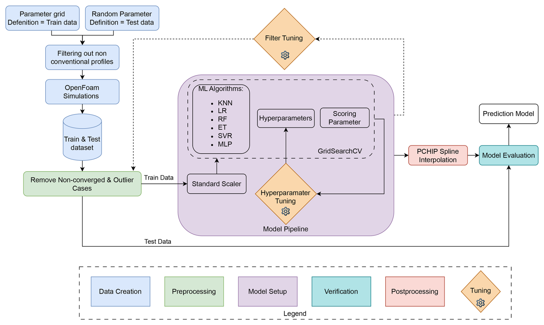
In the purple block, the model setup is illustrated. Building the ML model began with standardizing the filtered training datasets using a standard scaler to ensure consistent weighting of all input parameters. Multiple regression algorithms were then evaluated using their default settings (Pedregosa et al., 2011), with the selected models chosen for their strong baseline performance reported by Pandala (2021). Linear regression (LR) was also included for reference. The hyperparameters of the selected algorithms were subsequently optimized using a grid-search procedure with k-fold cross-validation, using the coefficient of determination R2 as the scoring metric. The dataset size was sufficient to allow reliable training–validation splits while still retaining a large and representative test set.
After hyperparameter tuning, the final models were evaluated on the independent test set. As the tree-based model response is piecewise constant in α, the outputs were additionally fitted with a PCHIP spline where a C1-continuous polar was required.
Table D1Overview of ML models, hyperparameters, and R2 values.
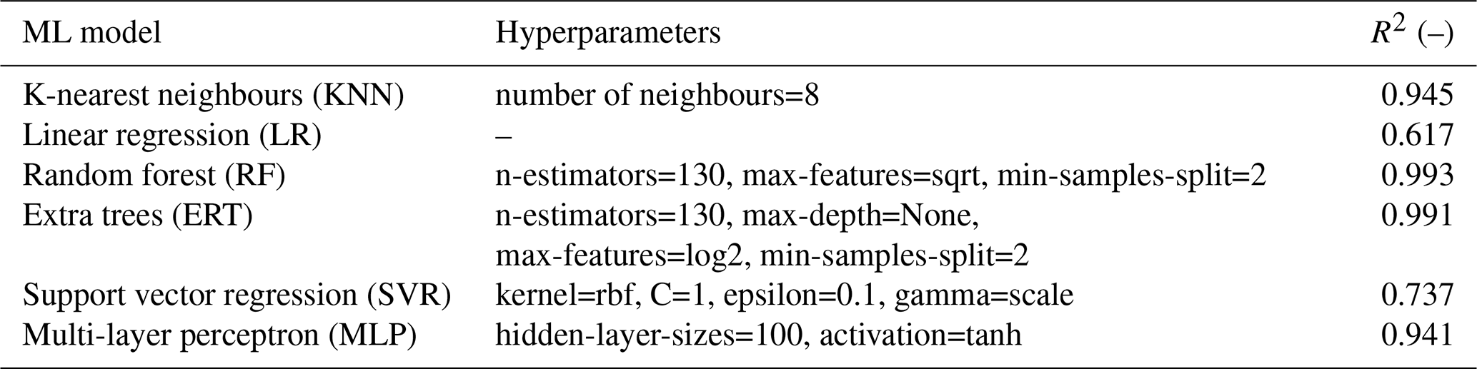
To quantify the Reynolds-number sensitivity across the three per-Re models, the polars of the three representative test profiles of Table 7 were evaluated with each model. Table D2 reports Cl and Cd at α= 6°, representative of the reel-out operating condition of the V3 kite flight in 2019 (Cayon et al., 2025). Across the factor of 20 in Re, Cl increases by 1 %–8 % while Cd decreases by 14 %–26 %. The drag reduction between Re = 1 × 10⁶ and 5 × 10⁶ corresponds to a fitted power-law exponent of approximately −0.145, in close agreement with the turbulent skin-friction scaling Cf∼ Re, although the decay flattens towards the highest Reynolds number. Across the operational band °, the three independently trained models remain closely spaced and consistently ordered; where the ordering is not strictly monotonic, the differences are within the regression uncertainty (Table 6). The largest sensitivity occurs at stall onset, where the stall angle increases with Re, consistent with expected boundary layer behaviour. The gradual, physically consistent variation across the sampled levels supports obtaining polars at intermediate Reynolds numbers via interpolation in log Re (Sect. 4).
Table D2Reynolds-number sensitivity of the per-Re ML models: predicted Cl and Cd at α= 6° for the test profiles of Table 7.
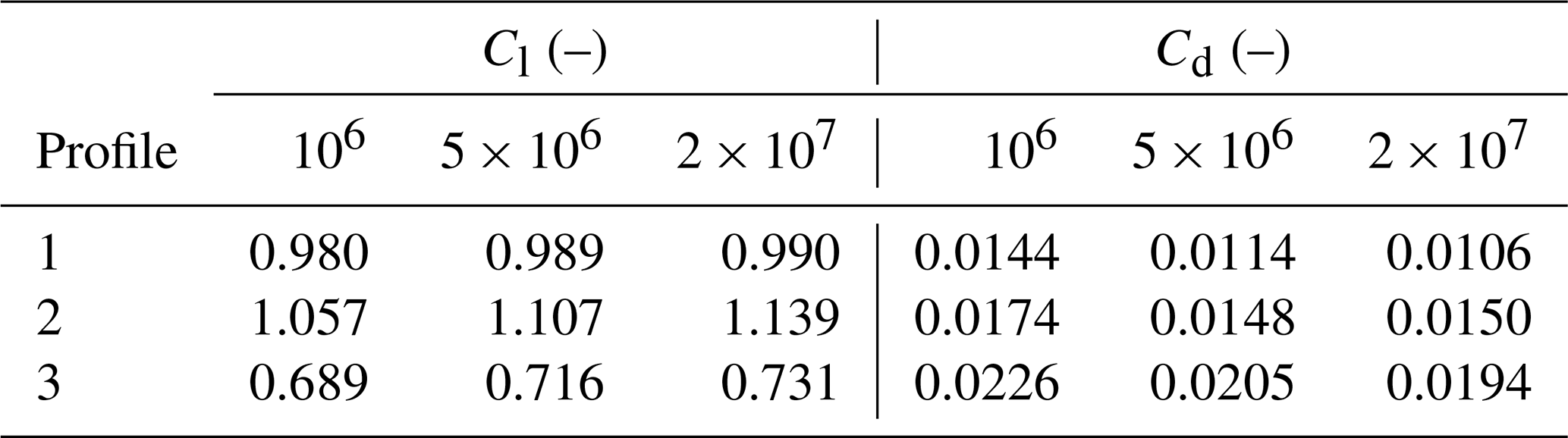
The geometric mesh of the TU Delft V3 kite is available on Zenodo at https://doi.org/10.5281/zenodo.15316036 (Poland et al., 2025a) and via https://awegroup.github.io/TUDELFT_V3_KITE/docs/datasets.html (last access: 19 October 2026) (which also contains more information and other datasets). The code for generating the diagrams in this paper is available on Zenodo at https://doi.org/10.5281/zenodo.18351807 (Poland et al., 2026c) or directly on GitHub at https://github.com/jellepoland/WES_aero_sim_for_kite_design (last access: 19 October 2026). The data supporting this paper, needed to run the code, are available through Zenodo at https://doi.org/10.5281/zenodo.18351331 (Poland et al., 2026d). The trained ML surrogate models, required to run the code and provided separately owing to their size (∼ 7 GB), are available on Zenodo at https://doi.org/10.5281/zenodo.16925758 (Poland et al., 2025b). The code relies on version 2.2.0 of the vortex-step method, available on GitHub at https://github.com/awegroup/Vortex-Step-Method (last access: 19 October 2026). The geometry, wind tunnel results, and polars used in Appendix B for the Belloc (2015) case are available at https://github.com/fairaero/Belloc-validation-data (last access: 19 October 2026) (last access: 16 February 2026).
JAWP compiled the original paper and performed the analysis shown in the results. KRGM performed the CFD and ML analysis, assisted in creating figures, and reviewed the paper. OC co-developed the latest version of the VSM, provided input to Sect. 6, and reviewed the paper several times. RS supervised the project and reviewed the paper.
At least one of the (co-)authors is a member of the editorial board of Wind Energy Science. The peer-review process was guided by an independent editor, and the authors also have no other competing interests to declare.
Publisher's note: Copernicus Publications remains neutral with regard to jurisdictional claims made in the text, published maps, institutional affiliations, or any other geographical representation in this paper. The authors bear the ultimate responsibility for providing appropriate place names. Views expressed in the text are those of the authors and do not necessarily reflect the views of the publisher.
We would like to thank https://fair.aero/ (last access: 19 October 2026) for open-sourcing the rigid paraglider data. We acknowledge the use of OpenAI's ChatGPT and Grammarly for assistance in refining the writing style of this paper.
This research has been supported by the Nederlandse Organisatie voor Wetenschappelijk Onderzoek (NWO grant no. 17628). This work has been partially supported by the MERIDIONAL project, which receives funding from the European Union’s Horizon Europe Programme (grant no. 101084216).
This paper was edited by Jens Nørkær Sørensen and reviewed by two anonymous referees.
Anderson, J., Corda, S., and Wie, D. V.: Numerical lifting line theory applied to drooped leading-edge wings below and above stall, J. Aircraft, 17, 898–904, https://doi.org/10.2514/3.44690, 1980. a
Barnes, J. P.: Semi-Empirical Vortex Step Method for the Lift and Induced Drag Loading of 2D or 3D Wings, in: Proceedings of the 1997 World Aviation Congress, Anaheim, CA, USA, https://doi.org/10.2514/6.1997-5559, 1997. a
Batchelor, G.: An Introduction to Fluid Dynamics, Cambridge University Press, https://doi.org/10.1017/CBO9780511800955, 1967. a, b
Belloc, H.: Wind Tunnel Investigation of a Rigid Paraglider Reference Wing, J. Aircraft, 52, 703–708, https://doi.org/10.2514/1.C032513, 2015. a, b
Bhagwat, M. J. and Leishman, J. G.: Generalized Viscous Vortex Model for Application to Free-Vortex Wake and Aeroacoustic Calculations, in: Proceedings of the 58th Annual Forum and Technology Display of the American Helicopter Society International, https://www.researchgate.net/publication/255470975_Generalized_viscous_vortex_model_for_application_to_free-vortex_wake_and_aeroacoustic_calculations (last access: 16 February 2026), 2002. a
Bosch, A., Schmehl, R., Tiso, P., and Rixen, D.: Dynamic nonlinear aeroelastic model of a kite for power generation, Journal of Guidance, Control and Dynamics, 37, 1426–1436, https://doi.org/10.2514/1.G000545, 2014. a
Branlard, E., Brownstein, I., Strom, B., Jonkman, J., Dana, S., and Baring-Gould, E. I.: A multipurpose lifting-line flow solver for arbitrary wind energy concepts, Wind Energ. Sci., 7, 455–467, https://doi.org/10.5194/wes-7-455-2022, 2022. a
Braslow, A. and Knox, E.: Simplified method for determining critical height of distributed roughness particles for boundary-layer transition, Tech. Rep. TN 4363, NACA, https://ntrs.nasa.gov/citations/19930085292 (last access: 16 February 2026), 1958. a
Breukels, J.: An Engineering Methodology for Kite Design, Ph.D. thesis, Delft University of Technology, http://resolver.tudelft.nl/uuid:cdece38a-1f13-47cc-b277-ed64fdda7cdf (last access: 6 April 2026), 2011. a, b
Breukels, J., Schmehl, R., and Ockels, W.: Aeroelastic Simulation of Flexible Membrane Wings based on Multibody System Dynamics, in: Airborne Wind Energy, edited by: Ahrens, U., Diehl, M., and Schmehl, R., Green Energy and Technology, 287–305, Springer, Berlin Heidelberg, https://doi.org/10.1007/978-3-642-39965-7_16, 2013. a
Candade, A. A., Ranneberg, M., and Schmehl, R.: Aero-structural Design of Composite Wings for Airborne Wind Energy Applications, J. Phys.-Conf. Ser., 1618, 032016, https://doi.org/10.1088/1742-6596/1618/3/032016, 2020. a
Castro-Fernández, I., Sánchez-Arriaga, G., and García-Villalba, M.: A review of the aerodynamics of airborne wind energy systems, Progress in Aerospace Sciences, 161, 101157, https://doi.org/10.1016/j.paerosci.2025.101157, 2026. a
Cayon, O., Gaunaa, M., and Schmehl, R.: Fast Aero-Structural Model of a Leading-Edge Inflatable Kite, Energies, 16, 3061, https://doi.org/10.3390/en16073061, 2023. a, b, c, d
Cayon, O., van Deursen, V., and Schmehl, R.: Translational dynamics of bridled kites: a reduced-order model in the course reference frame, Wind Energ. Sci., 11, 1097–1121, https://doi.org/10.5194/wes-11-1097-2026, 2026. a, b
Cayon, O., Watson, S., and Schmehl, R.: Kite as a sensor: wind and state estimation in tethered flying systems, Wind Energ. Sci., 10, 2161–2188, https://doi.org/10.5194/wes-10-2161-2025, 2025. a, b, c, d, e, f, g
Chattot, J.-J.: Analysis and design of wings and wing/winglet combinations at low speeds, in: Proceedings of the 42nd AIAA Aerospace Sciences Meeting and Exhibit, Reno, NV, USA, https://doi.org/10.2514/6.2004-220, 2004. a
Damiani, R., Wendt, F., Jonkman, J., and Sicard, J.: A Vortex Step Method for Nonlinear Airfoil Polar Data as Implemented in KiteAeroDyn, in: Proceedings of the AIAA Scitech 2019 Forum, San Diego, CA, USA, https://doi.org/10.2514/6.2019-0804, 2019. a, b, c, d, e, f
Deaves, M.: An Investigation of the Non-Linear 3D Flow Effects Relevant for Leading Edge Inflatable Kites, Master's thesis, Delft University of Technology, https://resolver.tudelft.nl/uuid:ccb56154-0b70-4a41-8223-24b0f8d145c5 (last access: 16 February 2015), 2015. a
Dekking, F., Kraaikamp, C., Lopuhaä, H., and Meester, L.: A Modern Introduction to Probability and Statistics: Understanding Why and How, Springer, London, 1st edn., https://doi.org/10.1007/1-84628-168-7, 2005. a, b
Den Boer, R.: Low Speed Aerodynamic Characteristics of a Two-Dimensional Sail Wing with Adjustable Slack of the Sail, Tech. Rep. LR-307, Technische Hogeschool Delft, Luchtvaart- en Ruimtevaarttechniek, https://resolver.tudelft.nl/uuid:18ae2cc6-434e-49c8-9296-d3fa450850a5 (last access: 16 February 2026), 1980. a
Dias, J. N.: Nonlinear lifting-line algorithm for unsteady and post-stall conditions, in: Proceedings of the 34th AIAA Applied Aerodynamics Conference, 1–11, Washington, DC, USA, https://doi.org/10.2514/6.2016-4164, 2016. a
Dorn, N. H. V. and DeYoung, J.: A Comparison of Three Theoretical Methods of Calculating Span Load Distribution on Swept Wings, Tech. Rep. Technical Note 1476, National Advisory Committee for Aeronautics (NACA), https://ntrs.nasa.gov/citations/19930082478 (last access: 4 January 2026), 1947. a
Drela, M.: XFOIL Subsonic Airfoil Development, https://web.mit.edu/drela/Public/web/xfoil/ (last access: 16 February 2026), 2013. a, b, c
Duport, C.: Modeling with consideration of the fluid-structure interaction of the behavior under load of a kite for auxiliary traction of ships, Ph.D. thesis, University of Bretagne, https://theses.hal.science/tel-02383312 (last access: 21 April 2026), 2018. a
Duport, C., Leroux, J.-B., Roncin, K., Jochum, C., and Parlier, Y.: Benchmarking of a 3D non-linear lifting line method against 3D RANSE simulations, La Houille Blanche, 105, 70–73, https://doi.org/10.1051/lhb/2019029, 2019. a
Elfert, C., Göhlich, D., and Schmehl, R.: Measurement of the turning behaviour of tethered membrane wings using automated flight manoeuvres, Wind Energ. Sci., 9, 2261–2282, https://doi.org/10.5194/wes-9-2261-2024, 2024. a
Etkin, B. and Reid, L. D.: Dynamics of Flight: Stability and Control, John Wiley & Sons, 3rd edn., ISBN 978-0-471-03418-8, 1996. a, b
Ferziger, J. H., Perić, M., and Street, R. L.: Computational Methods for Fluid Dynamics, Springer Nature Switzerland AG, Cham, Switzerland, 4th edn., https://doi.org/10.1007/978-3-319-99693-6, 2020. a
Folkersma, M., Schmehl, R., and Viré, A.: Boundary layer transition modeling on leading edge inflatable kite airfoils, Wind Energy, 22, 908–921, https://doi.org/10.1002/we.2329, 2019. a, b, c, d, e, f, g
Folkersma, M., Schmehl, R., and Viré, A.: Steady-State Aeroelasticity of a Ram-Air Wing for Airborne Wind Energy Applications, J. Phys.-Conf. Ser., 1618, 032018, https://doi.org/10.1088/1742-6596/1618/3/032018, 2020. a
Folkersma, M. A. M.: Aeroelasticity of Membrane Kites, Ph.D. thesis, Delft University of Technology, https://doi.org/10.4233/uuid:eae39f5a-49bc-438b-948f-b6ab51208068, 2022. a
Fransson, J. H. M., Matsubara, M., and Alfredsson, P. H.: Transition induced by free-stream turbulence, J. Fluid Mech., 527, 1–25, https://doi.org/10.1017/S0022112004002770, 2005. a
Fritz, E. K.: Swept Away: Numerical and Experimental Investigations into Swept Wind Turbine Blades, Ph.D. thesis, Delft University of Technology, https://doi.org/10.4233/uuid:55415991-053c-4c74-b31a-3db8724bfab7, 2024. a
Gallay, S. and Laurendeau, E.: Nonlinear generalized lifting-line coupling algorithms for pre/poststall flows, AIAA Journal, 53, 1784–1792, https://doi.org/10.2514/1.J053530, 2015. a
Garrel, A. V.: Development of a Wind Turbine Aero-Module for FOCUS, Tech. rep., Energy Research Centre of the Netherlands (ECN), https://publications.ecn.nl/ECN-C--03-079 (last access: 16 February 2026), 2003. a
Gaunaa, M., Li, Y., Pirrung, G., Kallesøe, B. S., and Madsen, H. A.: A correction model for the effect of spanwise flow on the viscous force contribution in BEM and Lifting Line methods, J. Phys.-Conf. Ser., 2767, 022068, https://doi.org/10.1088/1742-6596/2767/2/022068, 2024. a
Gaunaa, M., Carqueija P. F. P., Réthoré, P.-E., and Sørensen, N. N.: A Computationally Efficient Method for Determining the Aerodynamic Performance of Kites for Wind Energy Applications, in: EWEA Annual Event 2011, European Wind Energy Association (EWEA), https://backend.orbit.dtu.dk/ws/portalfiles/portal/6241674/Gaunaa_poster_EWEA2011presentation[1].pdf (last access: 16 February 2026), 2011. a
Goates, C. and Hunsaker, D.: Practical Implementation of a General Numerical Lifting-Line Method, in: AIAA Scitech 2021 Forum, https://doi.org/10.2514/6.2021-0118, 2021. a
Hummel, J., Göhlich, D., and Schmehl, R.: Automatic measurement and characterization of the dynamic properties of tethered membrane wings, Wind Energ. Sci., 4, 41–55, https://doi.org/10.5194/wes-4-41-2019, 2019. a
Hunsaker, D.: Post stall behavior of a lifting line algorithm, https://digitalcommons.usu.edu/mae_facpub/103/ (last access: 12 August 2025), 2007. a
Jain, I., Katiyar, S., and Sarkar, S.: Influence of Varying Freestream Turbulence on Flow Transition Over Distributed Surface Roughness, in: Proceedings of the ASME Turbo Expo 2024: Turbomachinery Technical Conference and Exposition, GT2024, V12CT32A018, ASME, https://doi.org/10.1115/GT2024-124283, 2024. a
Jonkman, J.: Google/Makani Energy Kite Modeling; Cooperative Research and Development Final Report, Tech. Rep. CRD-18-00569 NREL/TP-5000-80635, National Renewable Energy Laboratory, https://docs.nlr.gov/docs/fy21osti/80635.pdf (last access: 16 February 2026), 2021. a, b
Kappel, R. V.: Aerodynamic analysis tool for dynamic leading edge inflated kite models: a nonlinear vortex lattice method, Master's thesis, Delft University of Technology, https://resolver.tudelft.nl/uuid:385d316b-c997-4a02-b0f3-b30c40fffc32 (last access: 16 February 2026), 2012. a, b
Kitepower: Kitepower; Airborne Wind Energy; Plug and Play, Mobile Wind Energy, https://thekitepower.com/ (last access: 9 January 2025), 2025. a
Kutta, M. W.: Auftriebskräfte in strömenden Flüssigkeiten, Illustrierte Aeronautische Mitteilungen, 6, 133, 1902. a
Leloup, R., Roncin, K., Bles, G., Leroux, J. B., Jochum, C., and Parlier, Y.: Estimation of the lift-to-drag ratio using the lifting line method: Application to a leading edge inflatable kite, in: Airborne Wind Energy, edited by: Ahrens, U., Schmehl, R., and Diehl, M., 339–355, Springer, https://doi.org/10.1007/978-3-642-39965-7_19, 2013. a
Leuthold, R.: Multiple-Wake Vortex Lattice Method for Membrane Wing Kites, Master's thesis, Delft University of Technology, http://resolver.tudelft.nl/uuid:4c2f34c2-d465-491a-aa64-d991978fedf4 (last access: 16 February 2026), 2015. a, b
Li, A., Gaunaa, M., Pirrung, G. R., Meyer Forsting, A., and Horcas, S. G.: How should the lift and drag forces be calculated from 2-D airfoil data for dihedral or coned wind turbine blades?, Wind Energ. Sci., 7, 1341–1365, https://doi.org/10.5194/wes-7-1341-2022, 2022. a, b, c, d, e, f
Lolies, T., Gourdain, N., Charlotte, M., and Goldsmith, B.: Numerical Methods for Efficient Fluid–Structure Interaction Simulations of Paragliders, Aerotec. Missili Spaz., 98, 221–229, https://doi.org/10.1007/s42496-019-00017-2, 2019. a
Loyd, M. L.: Crosswind kite power (for large-scale wind power production), J. Energy, 4, 106–111, https://doi.org/10.2514/3.48021, 1980. a
Masure, K.: Regression Model of Leading Edge Inflatable Kite Profile Aerodynamics, Master's thesis, Delft University of Technology, https://resolver.tudelft.nl/uuid:865d59fc-ccff-462e-9bac-e81725f1c0c9 (last access: 16 February 2026), 2025. a, b, c, d, e, f, g, h, i
Menter, F. R.: Two-equation eddy-viscosity turbulence models for engineering applications, AIAA Journal, 32, 1598–1605, https://doi.org/10.2514/3.12149, 1994. a
Mukherjee, R. and Gopalarathnam, A.: Poststall prediction of multiple-lifting-surface configurations using a decambering approach, J. Aircraft, 43, 660–668, https://doi.org/10.2514/1.15149, 2006. a
Oehler, J. and Schmehl, R.: Aerodynamic characterization of a soft kite by in situ flow measurement, Wind Energ. Sci., 4, 1–21, https://doi.org/10.5194/wes-4-1-2019, 2019. a
OpenFOAM: OpenFOAM, OpenCFD [code], https://www.openfoam.com/ (last access: 16 February 2026), 2006. a
Pandala, S.: lazypredict: Lazy Machine Learning, GitHub [code], https://github.com/shankarpandala/lazypredict (last access: 16 February 2026), 2021. a, b
Pedregosa, F., Varoquaux, G., Gramfort, A., Michel, V., Thirion, B., Grisel, O., Blondel, M., Prettenhofer, P., Weiss, R., Dubourg, V., Vanderplas, J., Passos, A., Cournapeau, D., Brucher, M., Perrot, M., and Duchesnay, E.: Scikit-learn: Machine Learning in Python, J. Mach. Learn. Res., 12, 2825–2830, 2011. a, b
Phillips, W. F. and Snyder, D. O.: Modern Adaptation of Prandtl’s Classic Lifting-Line Theory, J. Aircraft, 37, 662–670, https://doi.org/10.2514/2.2649, 2000. a, b
Pistolesi, E.: Aerodinamica, Biblioteca dell'Ingegnere, Scienze Propedeutiche, I, Unions Tipografica Editrice Torinese, https://openlibrary.org/works/OL8269760W/Aerodinamica?edition=key:/books/OL6290732M (last access: 16 February 2026), 1932. a
Piszkin, S. T. and Levinsky, E. S.: Nonlinear Lifting Line Theory for Predicting Stalling Instabilities on Wings of Moderate Aspect Ratio, Tech. Rep. AD-A027 645, General Dynamics/Convair, https://apps.dtic.mil/sti/citations/ADA027645 (last access: 16 February 2026), 1976. a, b
Pointwise: Fidelity Pointwise [code], https://www.cfd-technologies.co.uk/fidelity-pointwise/ (last access: 16 February 2026), 2025. a
Poland, J. A. W., Lebesque, G., Schmehl, R., and Viré, A.: Surface mesh of the TUDELFT_V3_KITE CAD with edge fillets, in: Wind Energy Science (Version 0.0.1, Issue -), Zenodo [data set], https://doi.org/10.5281/zenodo.15316036, 2025a. a
Poland, J. A. W., Masure, K. R. G., and Schmehl, R.: Machine learning models for leading-edge inflatable airfoil aerodynamics, Zenodo [data set], https://doi.org/10.5281/zenodo.16925759, 2025b. a
Poland, J. A. W., Fritz, E., and Schmehl, R.: Flow field analysis of a leading-edge inflatable kite rigid-scale model using stereoscopic particle image velocimetry, Wind Energ. Sci., 11, 1461–1485, https://doi.org/10.5194/wes-11-1461-2026, 2026a. a, b
Poland, J. A. W., van Spronsen, J. M., Gaunaa, M., and Schmehl, R.: Wind tunnel load measurements of a leading-edge inflatable kite rigid-scale model, Wind Energ. Sci., 11, 911–936, https://doi.org/10.5194/wes-11-911-2026, 2026b. a, b, c, d, e, f, g, h, i
Poland, J. A. W., Masure, K. R. G., Cayon, O., and Schmehl, R.: Computational aerodynamics for soft-wing kite design (Version v1.0.2), Zenodo [code], https://doi.org/10.5281/zenodo.18351808, 2026. a
Poland, J. A. W., Schmehl, R., Cayón Domingo, O., and Masure, K. R. G.: Supporting dataset to analysis code, use to generate figures for the paper: “Computational aerodynamics for leading-edge inflatable kite design”, in: Wind Energy Science, Zenodo [data set], https://doi.org/10.5281/zenodo.18351331, 2026d. a
Prandtl, L.: Tragflügeltheorie, I. Mitteilung, Nachrichten von der Gesellschaft der Wissenschaften zu Göttingen, Mathematisch-Physikalische Klasse, 1918, 451–477, http://eudml.org/doc/59036 (last access: 16 February 2026), 1918. a
Ranneberg, M.: Direct Wing Design and Inverse Airfoil Identification with the Nonlinear Weissinger Method, https://doi.org/10.48550/arXiv.1501.04983, 2015. a, b, c, d, e
Sharpe, P.: NeuralFoil: An airfoil aerodynamics analysis tool using physics-informed machine learning, GitHub [code], https://github.com/peterdsharpe/NeuralFoil (last access: 16 February 2026), 2023. a
Sharpe, P. D.: Accelerating Practical Engineering Design Optimization with Computational Graph Transformations, Ph.D. thesis, Massachusetts Institute of Technology, https://hdl.handle.net/1721.1/157809 (last access: 8 July 2025), 2024. a, b
Simonet, T., Roncin, K., Faure, T., and Daridon, L.: An Efficient 3D Non-Linear Lifting-Line Method with Correction for Post-Stall Regime, Research Square [preprint], https://doi.org/10.21203/rs.3.rs-3955527/v1, in review, 2026. a, b
Tani, I.: A Simple Method of Calculating the Induced Velocity of a Monoplane Wing, Bulletin of the Aeronautical Research Institute, Tokyo Imperial University, 9, 64–76, https://jaxa.repo.nii.ac.jp/records/35482 (last access: 16 February 2026), 1934. a
Thedens, P.: An integrated aero-structural model for ram-air kite simulations: with application to airborne wind energy, Ph.D. thesis, Delft University of Technology, https://doi.org/10.4233/uuid:16e90401-62fc-4bc3-bf04-7a8c7bb0e2ee, 2022. a
Van der Vlugt, R., Bley, A., Noom, M., and Schmehl, R.: Quasi-steady model of a pumping kite power system, Renew. Energ., 131, 83–99, https://doi.org/10.1016/j.renene.2018.07.023, 2019. a
van Lith, T. L. B., Poland, J. A. W., Watson, S. J., and Schmehl, R.: Aerodynamic analysis of a two-dimensional rigid leading edge inflatable airfoil, J. Phys.-Conf. Ser., 3224, 092024, https://doi.org/10.1088/1742-6596/3224/9/092024, 2026. a, b, c, d, e, f, g
Viré, A., Demkowicz, P., Folkersma, M., Roullier, A., and Schmehl, R.: Reynolds-averaged Navier-Stokes simulations of the flow past a leading edge inflatable wing for airborne wind energy applications, J. Phys.-Conf. Ser., 1618, 032007, https://doi.org/10.1088/1742-6596/1618/3/032007, 2020. a, b, c, d, e, f, g
Viré, A., Lebesque, G., Folkersma, M., and Schmehl, R.: Effect of Chordwise Struts and Misaligned Flow on the Aerodynamic Performance of a Leading-Edge Inflatable Wing, Energies, 15, 1450, https://doi.org/10.3390/en15041450, 2022. a, b, c, d, e, f, g, h, i, j
Watchorn, P.: Aerodynamic Load Modelling for Leading Edge Inflatable Kites, Master's thesis, Delft University of Technology, https://resolver.tudelft.nl/uuid:42f611a2-ef79-4540-a43c-0ea827700388 (last access: 16 February 2026), 2023. a, b, c, d, e
Weissinger, J.: The Lift Distribution of Swept-Back Wings, Tech. Rep. Technical Memorandum 1120, National Advisory Committee for Aeronautics (NACA), translation of Forschungsbericht 1553: Über die Auftriebsverteilung von Pfeilflügeln, https://ntrs.nasa.gov/citations/20030064148 (last access: 17 November 2025), 1947. a
Wick, B. H.: Study of the Subsonic Forces and Moments on an Inclined Plate of Infinite Span, Technical Note NACA-TN-3221, National Advisory Committee for Aeronautics, Washington, D.C., https://ntrs.nasa.gov/api/citations/19930084119/downloads/19930084119.pdf (last access: 16 February 2026), 1954. a
Zhang, Y., Zhou, Z., Wang, K., and Li, X.: Aerodynamic Characteristics of Different Airfoils under Varied Turbulence Intensities at Low Reynolds Numbers, Appl. Sci., 10, 1706, https://doi.org/10.3390/app10051706, 2020. a
- Abstract
- Introduction
- Vortex step method
- Airfoil aerodynamics
- Machine learning
- Results
- Aerodynamic design considerations
- Conclusions
- Appendix A: Profile distribution
- Appendix B: Evaluating force direction
- Appendix C: Assuming fully turbulent flow
- Appendix D: Machine learning model
- Code and data availability
- Author contributions
- Competing interests
- Disclaimer
- Acknowledgements
- Financial support
- Review statement
- References
- Abstract
- Introduction
- Vortex step method
- Airfoil aerodynamics
- Machine learning
- Results
- Aerodynamic design considerations
- Conclusions
- Appendix A: Profile distribution
- Appendix B: Evaluating force direction
- Appendix C: Assuming fully turbulent flow
- Appendix D: Machine learning model
- Code and data availability
- Author contributions
- Competing interests
- Disclaimer
- Acknowledgements
- Financial support
- Review statement
- References