A machine-learning-based approach for better prediction of fatigue life of offshore wind turbine foundations using smaller data sizes

As offshore wind turbine (OWT) foundations approach the end of their design life, the industry is increasingly focused on strategies for lifetime extension. As fatigue is the design driver for foundations of OWTs, reliable fatigue damage predictions are essential to support informed decisions for lifetime extensions. While simulation-based fatigue life reassessments are common, data-driven approaches using measured strain data have emerged as an alternative that can reduce modeling uncertainties. But, data-driven approaches face challenges, as having access to strain data over the entire past lifetime is not an industry standard. Often, measurement campaigns are only kicked off when a lifetime extension is considered, thus limiting the availability of strain data. However, environmental and operational conditions (EOCs) of the wind turbines are usually recorded during the whole operational period. Using limited strain measurements and long-term EOCs to estimate fatigue damage in unmonitored periods during the lifetime of the turbine requires temporal extrapolation techniques. Existing work on this topic presents several extrapolation methods, including linear time-based extrapolation, binning based on correlations between EOCs and average damage, and machine learning (ML) models. The accuracy of these methods depends on factors such as the selected EOC parameters, the duration and starting point of available strain data, the power rating and the type of the wind turbine, as well as the type and architecture of the extrapolation model used. This study presents a novel machine-learning-based extrapolation model using random forest (RF) for the temporal extrapolation of strain measurements. A comparative analysis of a novel RF model with previously identified binning models is presented. The extrapolation performance is validated using 5 years of measured strain, Supervisory Control and Data Acquisition (SCADA), and wave data from a 3 MW and a 9 MW OWT installed on monopile foundations in the Belgian North Sea. Using a sliding window approach on the available monitoring data, we estimate and compare the statistical uncertainty in fatigue life predictions of various extrapolation models. The results indicate that wave parameters play a more significant role in fatigue prediction for larger turbines of 9 MW compared to smaller ones of 3 MW power rating. For limited data sizes – less than 12 months – the proposed RF model demonstrates superior performance, offering more reliable fatigue life predictions with reduced statistical uncertainty. However, for longer datasets of greater than 12 months, the performance advantage of the RF model over binning methods becomes less pronounced. For 3 MW OWTs with datasets greater than 18 months, the RF model is outperformed by binning methods.

1 Introduction

As offshore wind farms mature, extending the operational lifetime of wind turbines has become a pressing concern for the wind energy industry. According to WindEurope (2017), a substantial share of the installed wind capacity in the European Union is expected to reach the end of its design life between 2020 and 2030. Decommissioning these assets without extending their service would hinder progress toward the EU's 2030 target of achieving 50 % of electricity from renewable sources. Therefore, lifetime extension, alongside re-powering and new installations, is vital for meeting long-term sustainability goals. As highlighted by Shafiee (2024), extending the operational life of OWTs offers significant economic and environmental benefits, including reduced levelized cost of energy (LCOE) and lower emissions.

Fatigue is a governing factor in the structural design of wind turbine support structures, which are primarily optimized for dynamic- rather than static-loading conditions (Sparrevik, 2019). Monopile foundations are typically designed for a service life of 20–25 years. However, findings from some structural health monitoring (SHM) campaigns suggest that actual fatigue loads may be lower than anticipated, revealing unexploited fatigue capacity and motivating detailed reassessments for lifetime extension purposes (Tewolde et al., 2018). For example, in the case of lifetime extension of the Samsø offshore wind farm in Denmark, the Danish Energy Agency required detailed fatigue reassessments using updated load conditions to support lifetime extension permits (Buljan, 2025). International guidelines for lifetime extension, such as those outlined in DNV (2016), recommend fatigue life reassessments based on updated models that incorporate measured environmental and operational data. Although traditional fatigue reassessments rely heavily on simulation-based models, the availability of measured strain, as typically provided by SHM systems, and long-term EOC data open the door for data-driven alternatives that can reduce uncertainties associated with initial design assumptions in the simulation-based models (Kinne and Thöns, 2023).

To support lifetime assessments, two primary approaches exist: simulation-based reassessments using updated models, and data-driven methods using measured strains. The latter mitigates modeling assumptions but introduces new challenges, such as the high cost of installation and maintenance of strain gauges on OWTs (Bezziccheri et al., 2017) and limited data availability (Pacheco et al., 2023). Strain gauges are typically installed at a few critical locations, requiring spatial extrapolation to predict strains at locations where no direct measurements are available. Strain measurements are limited in duration as having strain data over the entire past lifetime is not an industry standard and because of the challenges associated with traditional sensor deployment in harsh marine environments, such as sensor failures due to corrosion caused by saltwater and humidity, and high costs related to complex installation logistics (Encalada-Dávila et al., 2025). Often, measurement campaigns are only started when a lifetime extension is considered, thus limiting the availability of strain data. On the other hand, a Supervisory Control and Data Acquisition (SCADA) system is typically installed on OWTs to capture and record EOCs such as wind speed, power, rotational speed, etc., to enable the wind farm operators to track and control the turbine performance in real time (Moynihan et al., 2024). The available data pave the way for temporal extrapolation techniques that use limited strain measurements and long-term EOCs to estimate fatigue damage in unmonitored periods during the lifetime of a turbine.

Prior research has extensively explored the extrapolation of strain and load data for offshore wind turbines, both spatially, to uninstrumented locations, and temporally, beyond the measurement window. Spatial extrapolation studies include those targeting different positions on the same turbine (Ziegler et al., 2019; Moynihan et al., 2024; Fallais et al., 2025; Ziegler et al., 2017; Zou et al., 2023; Zhang et al., 2024; Simpson et al., 2025; Encalada-Dávila et al., 2025), as well as farm-wide extrapolation approaches where measurements from one or a few instrumented turbines, called fleet leaders, are extended to others across the farm (de N Santos et al., 2024; Weijtens et al., 2016; Noppe et al., 2020; Pacheco et al., 2023).

Temporal extrapolation methods vary in complexity, ranging from simple linear techniques to binning strategies that relate fatigue damage to EOCs to more advanced ML approaches. Notable studies have assessed the accuracy of these methods using various datasets (Hübler and Rolfes, 2022; Ziegler and Muskulus, 2016; Weijtens et al., 2016). For example, Hübler et al. (2018) evaluate linear extrapolation, also called 0-dimensional (0D) binning; 1D binning, where 10 min fatigue damage is split into wind speed bins; and 2D binning, splitting fatigue damage into wind speed and wind direction bins using strain measurements from a 3 MW OWT installed on a monopile. Hübler et al. (2018) conclude that strain measurements of 9 to 10 months provide a representative and unbiased dataset with 1D binning using wind speeds giving the most reliable fatigue life estimations. Hübler and Rolfes (2022) study the performance of multi-dimensional binning extrapolation, artificial neural networks (ANNs) and Gaussian process regression (GPR) trained using multiple 1-year periods of measured strains. In Hübler and Rolfes (2022), binning approaches using wind speed correlations provide the best results. Pacheco et al. (2022) summarize the steps for calculating and extrapolating fatigue damage in wind turbines using strain measurements. Apart from estimating the fatigue life of an instrumented turbine, Pacheco et al. (2022) conclude that the results from instrumented turbines can be extrapolated to uninstrumented turbines in the same wind farm. Pacheco et al. (2023) use a damage capture matrix formed using 2D binning in wind speed and turbulence intensity to extrapolate strain measurements from one turbine to other turbines in an onshore wind farm. Pacheco et al. (2023) recommend using 1-year monitoring periods and conclude that the uncertainties in extrapolations decrease with increasing monitoring periods.

The rapid development and advances in computer science and its applications in wind energy pose machine learning models as a favorable option for the temporal extrapolation of fatigue damage in wind turbines (He et al., 2022; Raju et al., 2025). Literature focuses on using ML models as surrogates trained on simulated data to predict fatigue loads on each turbine in a wind farm (Bossanyi, 2022; Gasparis et al., 2020; Singh et al., 2022). There is limited literature on the use of ML models trained on strain measurements and used for fatigue damage predictions such as de N Santos et al. (2023), who use physics-guided learning of neural networks trained on 9 months of strain measurements for long-term fatigue damage estimation using SCADA and acceleration data. In wind energy applications, the random forest (RF) model is proved to be a powerful ensemble learning method, widely used for regression and classification tasks. RF models adapt excellently to high-dimensional data and large-scale datasets, and are robust in dealing with missing values and unbalanced datasets (Karadeniz, 2025). For example, Karadeniz (2025) compares RF, long short-term memory network (LSTM) and gated recurrent unit (GRU) for predicting total harmonic distortion voltage (THDV) of offshore wind farms to conclude that RF models outperform LSTM and GRU in predicting THDV with lowest root mean squared error (RMSE). Similarly, Zhou et al. (2016) use an RF regression model to predict short-term power production of a wind farm and Rouholahnejad and Gottschall (2025) use an RF model to extrapolate near-surface wind speed up to 200 m.

A literature review highlights the fact that the sensitivity of ML- and binning-based extrapolation models to different turbine power ratings remains poorly understood. Many studies assume homogeneity in turbine design and operating conditions, often focusing on a single turbine type and neglecting spatial variability across the farm (Bouty et al., 2017). Consequently, it is unclear how extrapolation performance varies across turbines with different power ratings or environmental exposures.

Moreover, the validation of these models is often limited to short timescales (e.g., several months), which restricts confidence in their long-term predictive capability. Although several binning-based and regression-based methods have been proposed (Ziegler et al., 2017; Pacheco et al., 2023; Sadeghi et al., 2023b), their comparative effectiveness and robustness under varying data availability, input features, and turbine power ratings are not yet well established. Especially in discussions of lifetime extension for aging turbines, methodologies that require shorter measurement campaigns are advantageous. This raises key questions like: what is the minimum duration of the monitoring period required for statistically reliable fatigue life predictions? and: can machine learning models reduce this monitoring period without sacrificing accuracy or increasing uncertainty?

Despite the increasing attention to data-driven extrapolation, key gaps remain in the literature:

• A systematic comparison of binning and machine learning, specifically random forest models – for fatigue life prediction across multiple turbine sizes – is missing.

• The relative importance of SCADA and wave parameter selection for these models to predict fatigue damage has not been thoroughly assessed for turbines of different power ratings.

• The ability of these models to predict fatigue damage across different directions (fore–aft, side–side, or single-sensor measurements) has not been thoroughly evaluated for turbines of varying capacities.

• The sensitivity of these models to data availability, including variations in dataset size and measurement start time, is underexplored.

While previous studies have compared binning approaches with machine learning models such as ANNs and GPR (Hübler and Rolfes, 2022; de N Santos et al., 2023), these comparisons were generally performed for a single turbine and often using relatively limited datasets. Similarly, earlier work has examined the sensitivity of data-driven fatigue extrapolation to dataset length and measurement start time (Hübler and Rolfes, 2022) but again typically for a single turbine. Consequently, a systematic evaluation of RF models across multiple turbine sizes using extensive monitoring data, together with a multi-directional assessment of model performance and parameter relevance, remains missing.

This study addresses these gaps by first introducing a novel ML-based extrapolation model using random forest for the temporal extrapolation of strain measurements. This model is compared with state-of-the-art temporal extrapolation techniques for fatigue life prediction and validated using 5 years of measured strain, SCADA, and wave data from two offshore wind turbines: a 3 MW and a 9 MW turbine, both installed on monopiles in the Belgian North Sea. We analyze the influence of dataset size, measurement start time, model dimensionality, and feature selection on extrapolation accuracy. Multiple configurations of random forest models are tested, including recursive feature elimination with cross-validation (RFECV) and state-specific modeling, to explore trade-offs between model complexity and predictive performance.

The findings provide new insights into the reliability, convergence behavior, and practical limitations of data-driven fatigue extrapolation models, offering valuable guidance for their deployment in support of lifetime extension assessments.

The remainder of the paper is structured as follows: it begins with the objective section, leading into the measurement setup for strain, collecting SCADA, and wave data. The paper then explains the methodology section. This section elaborates on model development, with a focus on feature selection and binning. The Methodology section describes the RF model and outlines the technique for statistical uncertainty estimation applicable to these extrapolation models and details the approach for damage extrapolation used in estimating fatigue life. The paper then concludes with a presentation of the results of fatigue lifetime predictions in various directions, along with discussions of the results.

2 Objective

Consider initiating a strain measurement campaign aimed at reassessing the fatigue life of OWT with the goal of extending their lifetime. How long should measurements be conducted to ensure a reliable estimate of fatigue life? The growing number of aging OWTs demands fast, reliable, and data-efficient methods to accurately predict their end of life (EOL). Addressing this question is important since it can result in reduced costs for prolonged measurement campaigns and more time-efficient fatigue life estimates. Precise predictions of fatigue life are essential for making informed lifetime extension decisions; however, this requires balancing the duration of measurement campaigns with both the financial costs of data acquisition and the accuracy of the predictions.

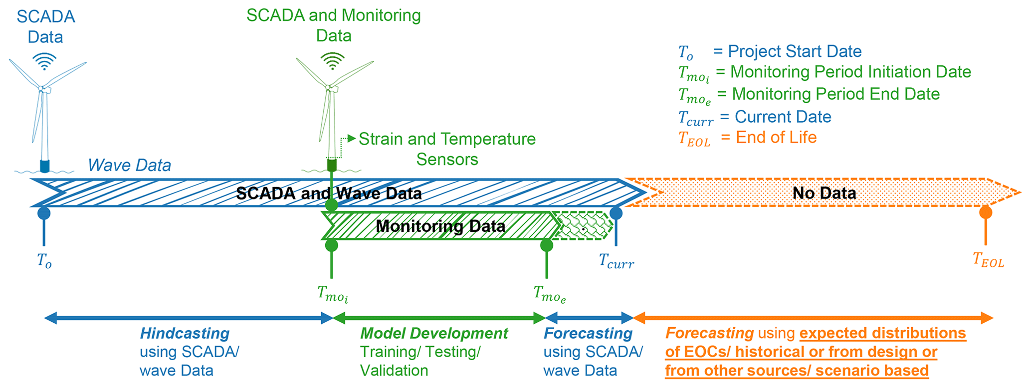
Figure 1 A timeline showing model developed using monitoring data used for hind-casting and forecasting using SCADA-wave data where available, and forecasting in future using expected distributions of EOCs.

Figure 1 illustrates the typical scenario encountered in fatigue life estimation. A strain sensor is installed at a later stage of the turbine's operation, for example, when lifetime extension is considered, initiating a monitoring period between $T_{{\mathrm{mo}}_{\mathrm{i}}}$ and $T_{{\mathrm{mo}}_{\mathrm{e}}}$. The shaded green region between $T_{{\mathrm{mo}}_{\mathrm{e}}}$ and T_curr indicates that the monitoring campaign may end before the current date. This represents the period for which no strain measurements are available. In cases where monitoring is still ongoing, $T_{{\mathrm{mo}}_{\mathrm{e}}}$ and T_curr coincide. Meanwhile, SCADA and wave data are usually available from the turbine's commissioning at T_o. During the monitoring period $\mathrm{\Delta }{T}_{\mathrm{m}}=T_{{\mathrm{mo}}_{\mathrm{e}}}-T_{{\mathrm{mo}}_{\mathrm{i}}}$, extrapolation models are trained/tested and validated using measured strain and corresponding SCADA/wave data. These models are then used to estimate cumulative fatigue damage up to the projected end-of-life time T_EOL, leveraging either historical SCADA/wave records or design-based EOC distributions. Such models can also facilitate the scenario-based forecasting of fatigue damage under varying operational profiles.

This study presents an ML-based extrapolation technique using RF models and systematically investigates the uncertainty in fatigue life predictions under varying monitoring periods and starting points. Given the seasonality of EOCs, the timing and length of the data window can significantly influence model robustness. In addition, factors such as binning strategies (e.g., dimensionality, bin resolution, empty-bin handling) and feature selection techniques in ML-based models play a critical role in the extrapolation accuracy.

Using long-term strain, SCADA, and wave measurements from two OWTs installed on monopiles, this study aims to do the following:

• Quantify the minimum monitoring duration ΔT_m required for reliable fatigue life predictions using ML and binning extrapolation models.

• Develop robust estimates of turbine end-of-life T_EOL using extrapolation models based on measured strain and EOCs data.

• Estimate uncertainty bounds associated with T_EOL under different modeling approaches.

• Evaluate the potential of machine learning models, random forests, to reduce the required monitoring durations and improve prediction reliability, in comparison to traditional extrapolation methods such as linear and binning-based models.

• Compare the performance of different extrapolation models across varying offshore wind turbine power ratings (3 and 9 MW) to assess model reliability.

• Compare the ability of these models to predict fatigue damage across different directions, fore–aft, side–side, or single-sensor measurements, and for turbines of different power ratings (3 and 9 MW).

3 Measurement setup

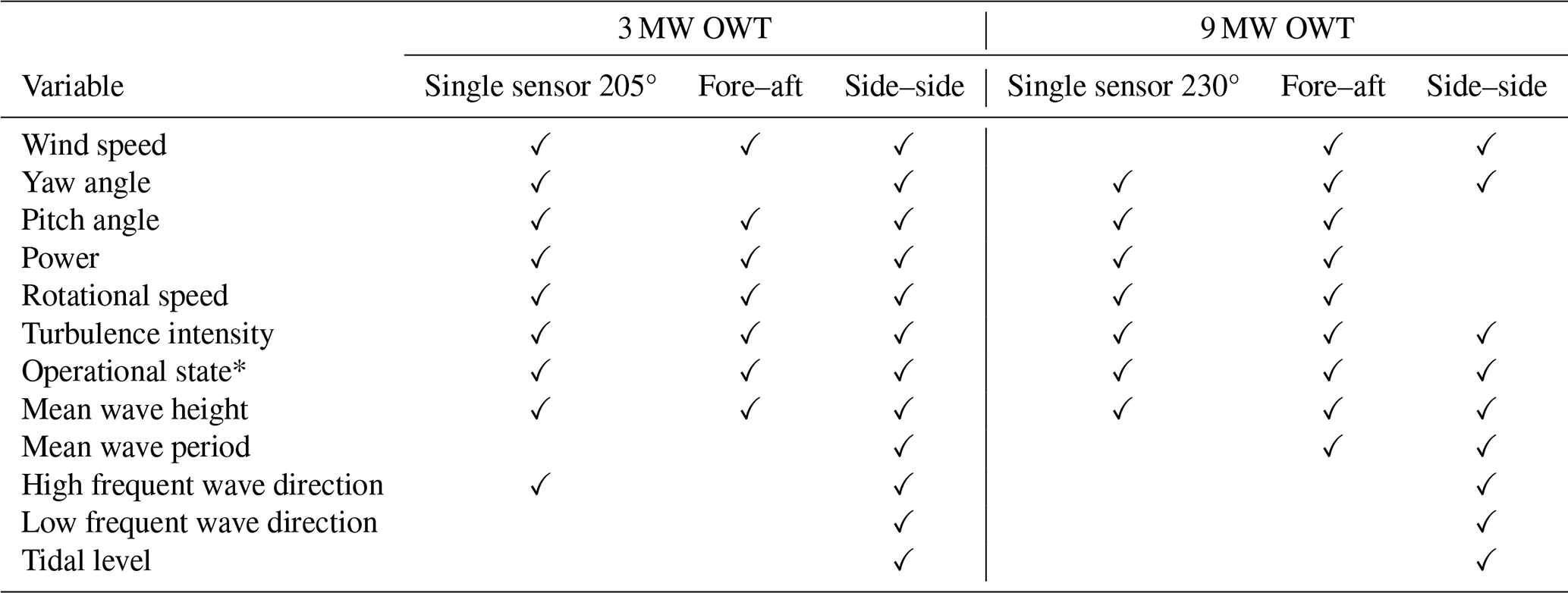
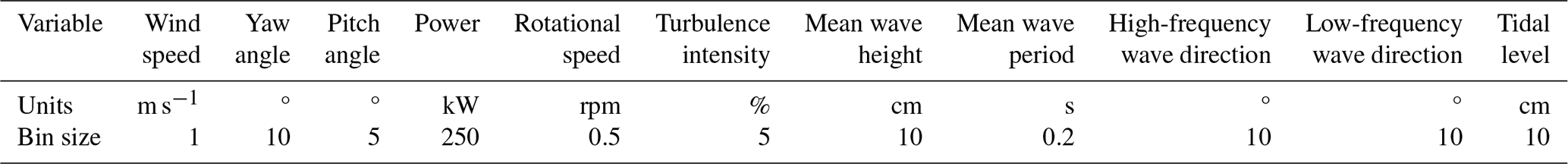
Table 1 provides an overview of the parameters used in this study along with the data availability. A total of 5 years of strain measurements, SCADA, and wave data from a 3 and 9 MW OWT are used. The strain measurement setup consists of six circumferential strain gauges installed on the transition piece (TP) near the tower–TP interface. Figure 2 presents the windrose diagrams for the 3 and 9 MW OWT, illustrating the probability distribution of wind occurrence across different directions. Figure 2 also shows the sensor locations positioned around the circumference, together with the dominant wind direction of 230°. The difference in windrose size reflects the actual relative monopile diameters: the smaller windrose on Fig. 2 (left) corresponds to a smaller diameter monopile for the 3 MW OWT, and the larger windrose on Fig. 2 (right) represents the larger diameter monopile of the 9 MW OWT. The sensor closest to the dominant wind direction is located at 205° for the 3 MW OWT and at 230° for the 9 MW OWT.

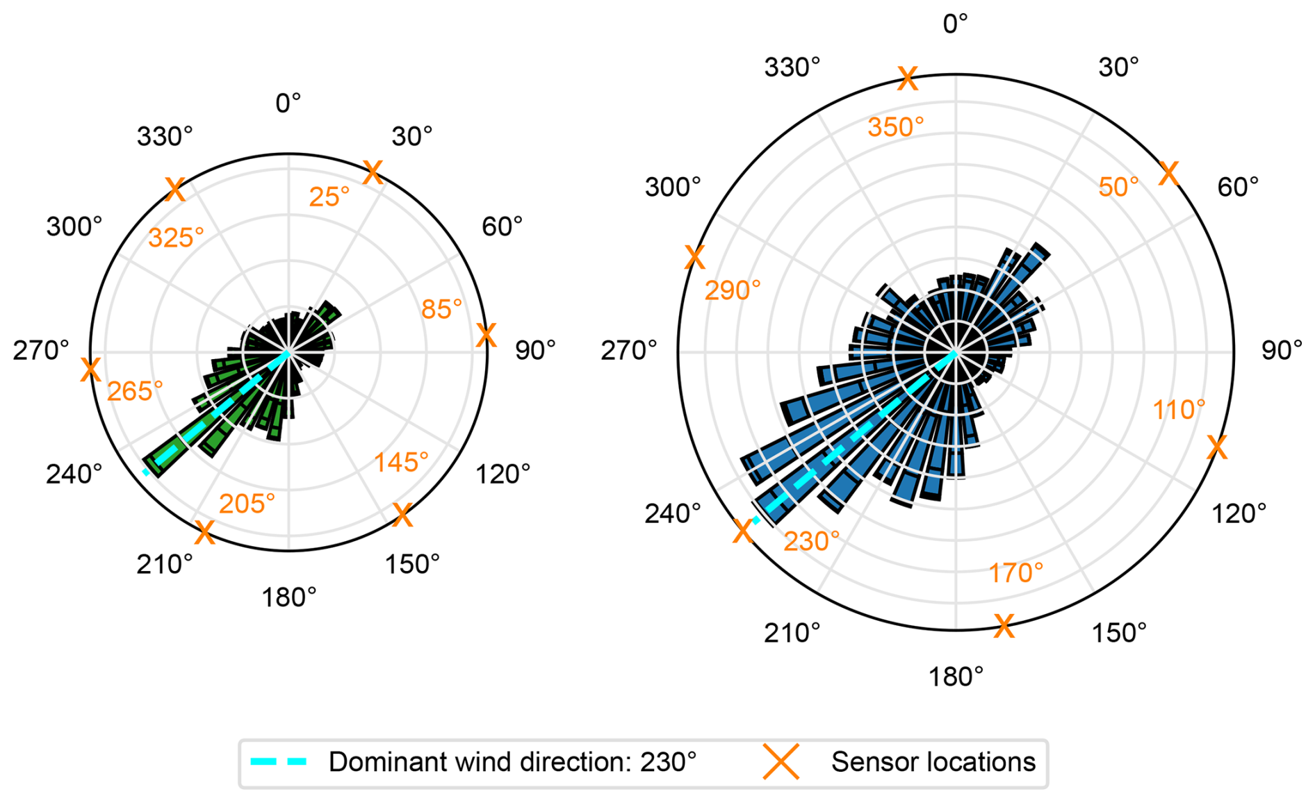
Figure 2 Location of sensors and windrose, showing the dominant wind direction for a 3 MW (left) and 9 MW (right) OWT.

3.1 Strain data

The data from six circumferential electrical strain gauges are pre-processed using the steps shown in Fig. 3. Each strain gauge is installed together with a dedicated thermocouple to enable temperature compensation. This temperature compensation as well as any long-term measurement drift is addressed through continuous follow-up and periodic recalibration of the strain gauges data by the SHM hardware supplier.

From the measured strains at the six circumferential sensors, the corresponding stresses and bending moments are obtained through a two-step procedure. First, the axial stress at each sensor location is computed using Hooke's law (Eq. 1).

$$\begin{array}{}\text{(1)}& {\mathit{\sigma }}_{zz,j}=E{\mathit{\epsilon }}_{zz,j},\end{array}$$

where E is Young's modulus, and ε_zz,j and σ_zz,j are the measured axial strain and resulting axial stress at the jth sensor, respectively. The general equation for normal stress σ_zz,j induced by a normal force F_N and global bending moments M_NS (north–south) and M_EW (east–west) in cylindrical coordinates is given by Eq. (2).

$$\begin{array}{}\text{(2)}& {\mathit{\sigma }}_{zz,j}={\displaystyle \frac{F_{\mathrm{N}}}{A}}+R_{\mathrm{i}}\left[{\displaystyle \frac{M_{\mathrm{NS}}}{I_{\mathrm{C}}}}\sin \left({\mathit{\theta }}_j\right)-{\displaystyle \frac{M_{\mathrm{EW}}}{I_{\mathrm{C}}}}\cos \left({\mathit{\theta }}_j\right)\right],\end{array}$$

where A is the cross-sectional area, R_i is the inner radius at the sensor location, I_C is the area moment of inertia, and θ_j is the clockwise angular position of the jth sensor from north–south axis. Equation (2) can be written for each sensor. With six sensors, this formulation yields an overdetermined system that is solved using a least-squares fitting procedure to estimate the normal load F_N and bending moments in both directions M_NS (north–south) and M_EW (east–west) from the measurements (see Sadeghi et al., 2023a; Link and Weiland, 2014, for more details).

The resulting bending moments are then rotated in fore–aft (FA) and side–side (SS) direction using Eq. (3).

$$\begin{array}{}\text{(3)}& \left\{\begin{array}{c}{M}_{\mathrm{FA}}\\ M_{\mathrm{SS}}\end{array}\right\}=\left[\begin{array}{cc}\cos (-\mathit{\psi }+\mathit{\pi })& \sin (-\mathit{\psi }+\mathit{\pi })\\ -\sin (-\mathit{\psi }+\mathit{\pi })& \cos (-\mathit{\psi }+\mathit{\pi })\end{array}\right]\left\{\begin{array}{c}{M}_{\mathrm{NS}}\\ M_{\mathrm{EW}}\end{array}\right\},\end{array}$$

where ψ is the mean yaw angle in each 10 min interval. This transformation yields the fore–aft (M_FA) and side–side (M_SS) bending moments, also defined as normal bending moment (M_tn) and lateral bending moment (M_tl), respectively, by the International Electrotechnical Commission (2021).

Stresses in fore–aft direction refer to axial stresses caused by the fore–aft bending moment (M_FA) and stresses in the side–side direction refer to axial stresses caused by the side–side bending moment (M_SS). Each 10 min signal is processed using rainflow cycle counting to get stress range histogram.

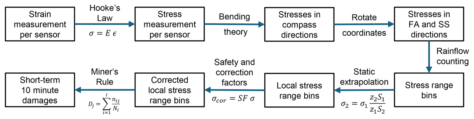
Figure 3 Strain data pre-processing to calculate short-term 10 min damages in the FA and SS directions (image reproduced from Hübler et al., 2018).

Stress range histograms or cycle count matrices are scaled using a combination of static extrapolation, safety, and correction factors. The static extrapolation factor is employed to project the measured stress signals onto fatigue-critical structural locations, without modeling structural dynamics. This factor is computed as the product of two ratios: (i) the bending moment ratio between the extrapolated and measured locations, obtained from bending moment diagrams either in design documentation or reanalysis; and (ii) the section modulus ratio at the two locations.

Additional correction factors include a stress concentration factor (SCF) as defined in DNV (2024) for various fatigue details, a material safety factor (MSF) as specified in relevant design guidelines such as the International Electrotechnical Commission (2019), and a thickness correction factor following the recommendations in DNV (2024) to account for the size effects. These factors are applied to generate a corrected stress range histogram for fatigue damage analysis. However, the exact numerical values of these scaling factors are not essential for the temporal extrapolation process and do not affect the conclusions of this paper (Hübler and Rolfes, 2022).

Subsequently, the fatigue damage corresponding to each stress range bin is computed using the appropriate S–N (Wöhler) curve described by Eq. (4) (Basquin, 1910), where $\log \left(\overline{a}\right)$ is the intercept term, m is the slope (or Wöhler exponent) of the S–N curve, Δσ is the stress range, and N is the number of cycles to failure.

$$\begin{array}{}\text{(4)}& \log \left(N\right)=\log \left(\overline{a}\right)-m\cdot \log \left(\mathrm{\Delta }\mathit{\sigma }\right)\end{array}$$

The slope (m) and intercept ($\log \left(\overline{a}\right)$) defining the S–N curve depend on the fatigue detail, environmental conditions, and material properties, and are provided in the DNV (2024) guidelines. In this study, the bilinear DNV D–A curve for a D-detail (circumferential butt weld made from both sides) is adopted, with slopes of $m=[\mathrm{3},\mathrm{5}]$ and intercepts of $\log \left(\overline{a}\right)=[\mathrm{12.164},\mathrm{15.606}]$, with a transition at 10⁷ cycles.

The individual damage contributions are calculated and accumulated over time using Palmgren–Miner's linear damage rule (Miner, 1945) to estimate the fatigue damage per 10 min interval, as shown in Eq. (5).

$$\begin{array}{}\text{(5)}& D=\sum _{i=\mathrm{1}}^k{\displaystyle \frac{n_i}{N_i}}\end{array}$$

where:

• n_i is the number of cycles in the ith stress range bin,

• N_i is the number of cycles to failure at the ith stress range (obtained from the S–N curve),

• k is the total number of stress range bins.

Fatigue damage of 10 min is used as the extrapolation model target variable. Strain data processing, cycle counting, stress range corrections, fatigue damage calculation, and accumulation are done using the open source python package py-fatigue (D'Antuono et al., 2023). In this study, fatigue life is estimated using three approaches based on damage values:

• Single-sensor damage. Fatigue life is estimated using damage calculated from the sensor nearest to the dominant wind direction. This approach bypasses the rotation of stress measurements and directional compass transformation (see Fig. 3), applying rainflow counting directly to the raw stress time series.

• Fore–aft (FA) damage. It is assumed that the turbine faces FA damage conditions throughout its lifetime. This method likely underestimates fatigue life as compared to a single sensor, since the FA damage state is not constantly maintained over time.

• Side–side (SS) damage. It is assumed that only SS damage prevails throughout the turbine lifetime. This approach allows the estimation of life consumption if SS damage states were persistent.

The methodology used to extrapolate damage predictions and estimate fatigue life (T_EOL) is described in detail in Sect. 4.3.

Table 1 Overview of SCADA, wave, and strain parameters for 3 and 9 MW OWT, their sources, duration, and availability factors.

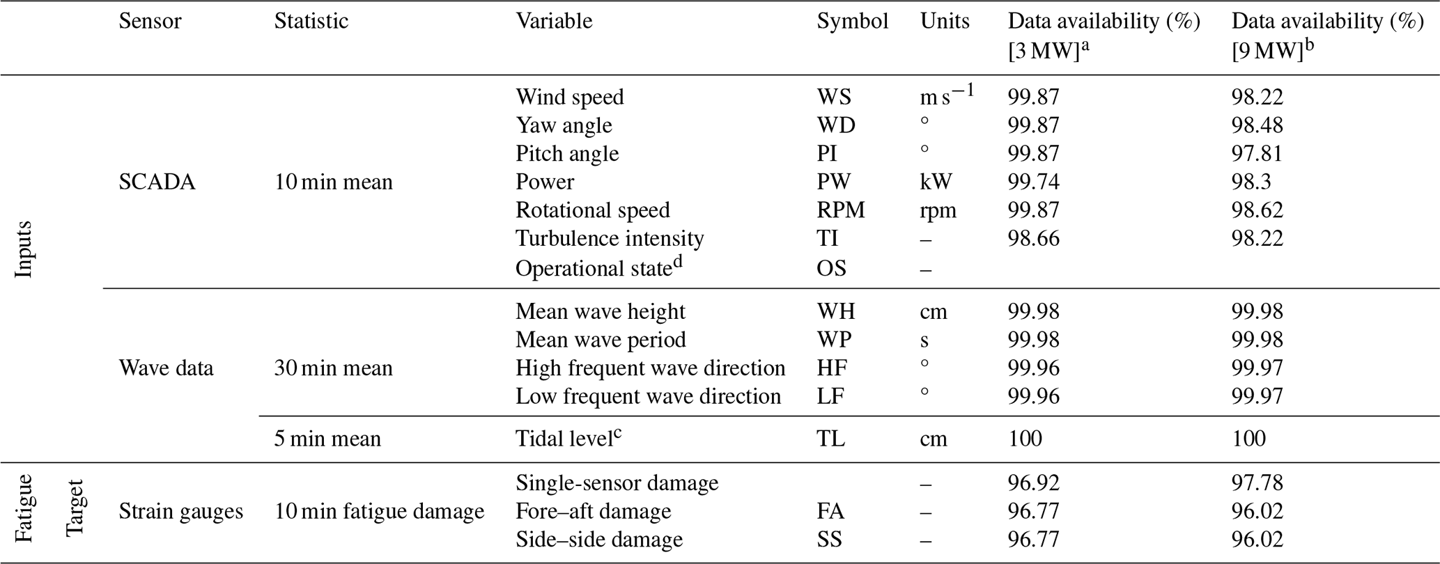
^a 5 years of monitoring and SCADA data used from 1 January 2020 to 31 December 2024. ^b 4.67 years of monitoring and SCADA data used from 1 May 2020 to 31 December 2024. ^c Tidal levels are taken from Ostend harbor – tide due to lower data availability for Wandelaar measuring pile (all other wave data are taken from a Thorntonbank South buoy). ^d Operational states for 3 MW “nominal”, “transient”, “idling”, and “high wind”. Operational states for 9 MW “nominal”, “transient”, “idling”, “high wind”, and “curtailed”.

3.2 SCADA and wave data

The SCADA system provides essential turbine parameters including wind speed, yaw angle, pitch angle, rotor power output, and rotational speed. The corresponding symbols used for these variables throughout this study are summarized in Table 1. Mean statistics of 10 min of these parameters are utilized as inputs for extrapolation model development.

Turbine operational states defined based on the 10 min SCADA statistics, including nominal, idling, high wind, curtailed (only for 9 MW OWT), and transient, are incorporated into both binning and ML-based extrapolation models. Intervals that occur during turbine transients (e.g., start-up, shutdown) fall outside the predefined statistical thresholds on SCADA statistics and are therefore labeled transient. For the 9 MW OWT, an additional curtailed operational state is identified, associated with curtailed power output, defined as intentional operation of the turbine at reduced power output to satisfy grid requirements. The nominal power generation and idling (parked) operational states are defined consistently across both the 3 and 9 MW OWTs.

Turbulence intensity (TI) is computed for each 10 min interval using the ratio of the standard deviation to the mean wind speed, defined as

$$\begin{array}{}\text{(6)}& \text{TI}=\mathrm{100}\times \left({\displaystyle \frac{{\mathit{\sigma }}_{\mathrm{wind}\mathrm{speed}}}{{\mathit{\mu }}_{\mathrm{wind}\mathrm{speed}}}}\right)\end{array}$$

Wave and tidal data are typically not included in wind farm SCADA datasets. For this study, publicly available environmental data from the Meetnet Vlaamse Banken (Agency for Maritime Services and Coast, 2025), covering the Belgian part of the North Sea, are used. Meetnet Vlaamse Banken comprises wave buoys and measurement piles deployed across the North Sea, providing measurements of wind, wave, and tidal conditions. Reported wave characteristics include wave height, 10 % highest waves, height of waves with period greater than 10 s, high frequent wave direction, low frequent wave direction, average wave period, and tidal levels. These measurements are generally reported with a sampling frequency of 15–30 min and are resampled with interpolation to align with the 10 min resolution of SCADA measurements from OWTs.

Wave data from the Thorntonbank South buoy are selected for analysis, as this station offers high data availability during the study period and is geographically closest to the considered wind farms, having a distance of 18.5 km from 3 MW OWT and 7.8 km from 9 MW OWT. Although this location does not provide tidal data, tidal measurements from the Wandelaar station were evaluated but excluded due to the low data availability during the time of interest. Instead, tidal data from the Oostende station are used, as they align well with wave radar observations at one of the wind farms analyzed, of which a small window was available for validation. A potential time offset exists between wave events at the OWT site and the measurement station due to spatial separation. A simplified time-shift estimation, assuming deep-water wave propagation and direct travel from the buoy to the turbine location, yields a maximum offset of approximately 40 min. However, no explicit correction for wave-time offset is applied in this study. The distance between the turbine and the wave measurement buoy leads to some differences in wave parameters compared with measurements taken closer to the 9 MW turbine, although the overall temporal trends remain consistent. However, the acceptable distance between wave measurement station and turbine depends on local bathymetry and wave climate, and closer measurements may be required in areas with strong spatial gradients.

4 Methodology

Figure 4 illustrates an overview of the methodology, where various extrapolation models are applied to different monitoring period sizes and starting points. A selected monitoring window ΔT_m, with varying durations and starting points, is used to train extrapolation models. These models predict 10 min fatigue damage based on SCADA/wave parameters, which is used to estimate fatigue life T_EOL over the full operational timeline.

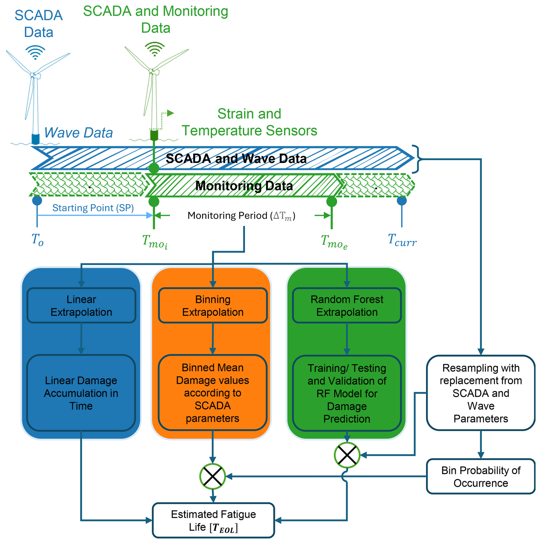
Figure 4 Five years of data T_curr−T_o are split into a sliding window of variable size ΔT_m and starting point (SP) used for models development. Fatigue life T_EOL is estimated using complete SCADA and wave data.

4.1 Model development

Two modeling approaches are investigated for fatigue life extrapolation: (1) multi-dimensional binning (Pacheco et al., 2022; Hübler et al., 2018; Hübler and Rolfes, 2022; Sadeghi et al., 2023b) and (2) the random forest model. The random forest model has been selected owing to its robustness and better performance relative to other machine learning models (Karadeniz, 2025; Rouholahnejad and Gottschall, 2025). This paper focuses on the fundamental question as to whether the deployment of ML models offers any significant benefits instead of comparing the performance of various ML models.

SCADA and wave statistics of 10 min are used as input parameters, and 10 min fatigue damage is the target variable, as summarized in Table 1. Extrapolation models are evaluated under varying monitoring durations and feature subsets to assess their robustness and prediction accuracy.

4.1.1 Feature selection

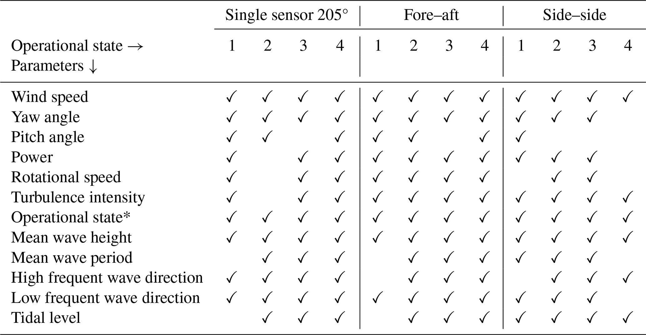
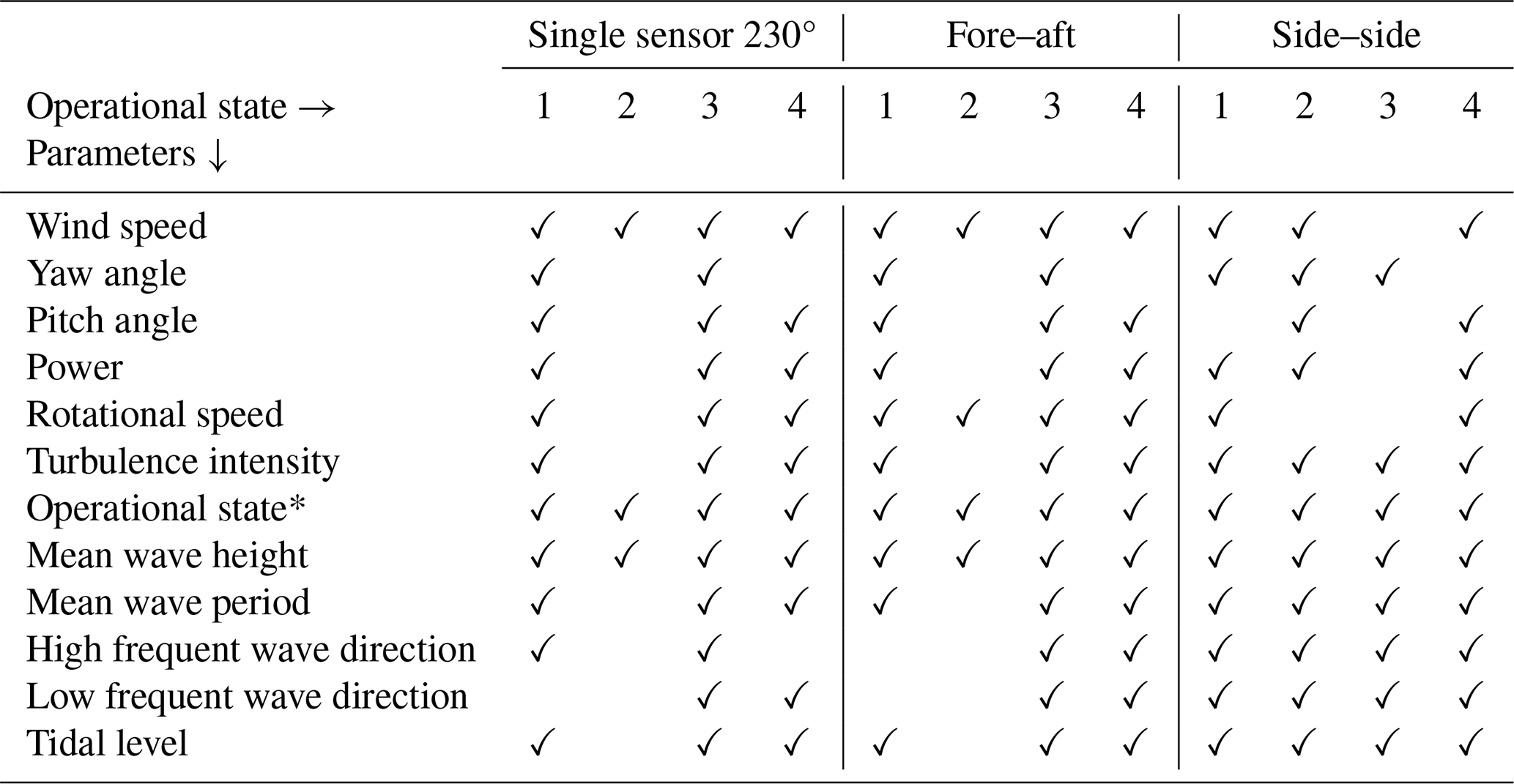
Feature selection is a crucial step, especially in fatigue modeling where input parameters – to be precise, the SCADA and wave data – may vary in importance depending on the operational state of the turbine and the size of the training dataset. Feature selection is performed for both the binning and RF models to enable a fair comparison by using the same set of input features. Four approaches to feature selection are employed:

1. Random forest feature importance. A filter-based method is applied using the built-in feature importance metric from a random forest model, which ranks input variables based on their contribution to reducing node impurity across all trees (see Breiman, 2001, 2002, for more details). This model is trained using the first 12 months of monitoring data. The top five features, capturing over 80 % of cumulative importance, are selected. This five-feature limit enables a fair comparison between a 5D binning approach and RF model using five features, denoted by RF-5D. Feature selection is performed separately for different fatigue targets, fore–aft, side–side, and single-sensor damage, since the relevance of features differs for these damage types. Categorical variables, such as turbine operational states, are transformed using one-hot encoding to enable their use in tree-based models.

2. Global RFECV. A recursive feature elimination with cross-validation (see Guyon et al., 2002, for details on RFECV methodology) is applied globally, i.e., across all operational states, using the same 12-month dataset. This method, referred to as global RFECV, aims to identify a reduced yet effective feature subset optimized for overall model performance.

3. State-specific RFECV. To account for operational state-dependent fatigue behavior, RFECV is applied individually to each turbine operational state, generating unique feature subsets per state. Separate random forest models are trained for each state, significantly increasing the number of models but allowing for tailored fatigue prediction.

4. Full-feature baseline. A baseline model using all available features is also developed to serve as an upper-bound benchmark, against which the performance of RF-5D and RFECV-based models is compared.

4.1.2 Binning extrapolation

In the binning approach, fatigue damage values are discretized based on selected EOC parameters. A single statistic, typically mean, is computed to represent all damage in each bin, resulting in a multi-dimensional damage matrix. To estimate long-term fatigue life, EOC parameters are sampled from extended operational periods to determine bin probabilities. These probabilities, representing the occurrence likelihood of EOCs, are combined with the damage matrix to compute the expected fatigue damage. To account for varying turbine operational states, the monitoring period ΔT_m is first segmented by operational states, and a separate damage matrix is constructed for each state. This allows the binning approach to accurately reflect state-dependent fatigue behavior.

In this paper, the dimensionality of binning is increased from 1D to 5D. In 1D binning, only wind speed is used if wind speed is in the selected features. This is because Hübler and Rolfes (2022) suggest that binning approaches using wind speed correlations provide best results. For 2D binning, wind speed along with the parameter with the highest importance, as determined by feature_importances_scores from a random forest model, is used for discretization. For higher dimensions, the top-ranked features are sequentially added-e.g., 3D binning uses wind speed and the top two features, 4D binning uses wind speed and the top three features, and so on, up to 5D.

Explicit bin size optimization is not performed in this study. Bin sizes for SCADA and wave parameters used in this paper are given in Appendix D. A critical challenge in multi-dimensional binning is the treatment of empty bins, which can arise due to data sparsity in high-dimensional feature spaces. For example, in 3D binning based on wind speed, wind direction, and power, certain combinations of bin values may not be observed within the monitoring period, particularly when the monitoring duration is short, resulting in empty bins. Several strategies have been proposed in the literature to address this issue.

For instance, Noppe et al. (2020) suggest filling empty bins with the maximum damage value observed in adjacent or neighboring bins, thereby maintaining conservative fatigue estimates. Pacheco et al. (2023) propose a more sophisticated interpolation approach, fitting a 3D surface to the damage matrix to estimate missing values. Simpler and more commonly applied methods include filling empty bins with the mean damage from samples in the same wind speed bin, the 90th percentile, or the maximum damage. For example, Hübler et al. (2018) suggest filling the empty bins with highest statistical damage value of the same wind speed bin but conclude that in this strategy, bins are filled up conservatively, leading to reduced lifetimes. However, Hübler and Rolfes (2022) adopt filling empty bins with the maximum value observed in the surrounding bins, as suggested by Noppe et al. (2020).

In this study, the performance of bins filling with mean, 90th percentile, and maximum damage value of the same wind speed bin is evaluated (see Fig. A1, Appendix A). Extreme values – such as the 90th percentile or maximum – tends to significantly overestimate fatigue damage, thus underestimating fatigue life. In contrast, mean-value bin filling yields more consistent and realistic fatigue predictions and is therefore adopted throughout this work.

4.1.3 Random forest model

Random forest is an ensemble learning method widely applied to regression and classification tasks. It enhances prediction accuracy and stability by constructing multiple decision trees and aggregating their outputs. Each tree is trained on a bootstrap sample, created by sampling with replacement from the original dataset, and, at each split, a random subset of features is considered to increase model diversity and reduce overfitting risk. RF models demonstrate strong adaptability to high-dimensional and large-scale datasets, as well as robustness in handling missing values, unbalanced data, noise, and outliers. Furthermore, RF inherently provides feature importance rankings, offering valuable insight into the relative contribution of input variables to the prediction outcome (Karadeniz, 2025).

The RF regression model is used to predict 10 min fatigue damage based on input SCADA and wave parameters. To handle categorical variables, turbine operational states, as described in Sect. 3.2, are transformed using one-hot encoding, converting each category into a separate binary feature. The target variable, 10 min damage, is normalized using a MinMaxScaler to scale values between 0 and 1, facilitating stable model training.

The RF model is trained using the open source python package Scikit-learn (Pedregosa et al., 2012), and a Bayesian optimization approach is employed for tuning the hyperparameters of the RF model using the Hyperopt package in python (Bergstra et al., 2013). The hyperparameter search space includes the number of estimators (n_estimators (10, 300)), maximum depth of trees (max_depth (2, 15)), minimum samples required to split a node (min_samples_split (2, 15)), and the minimum number of samples required at a leaf node (min_samples_leaf (1, 7)).

Bayesian optimization is performed with a maximum of 50 evaluations (max_evals=50) to identify the optimal set of hyperparameters. Each monitoring period ΔT_m is split into 80 % training and 20 % testing subsets to evaluate the model performance and generalizability.

4.2 Statistical uncertainty estimation

Statistical uncertainty in this paper refers to the scatter in fatigue life predictions by models trained using ΔT_m, but the starting point of ΔT_m could be anywhere within T_curr−T_o, as shown in Fig. 4. This aims to answer the question of how much the starting point (SP) of the measurement campaign influences the outcome on T_EOL after a campaign of ΔT_m months.

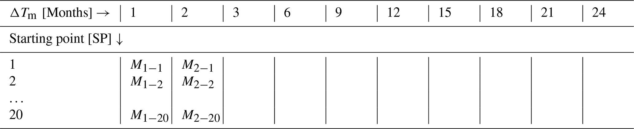
To achieve this, the monitoring period ΔT_m is varied from 1 month to 24 months to study the effect of varying data size on the model predictions. For each size of monitoring period ΔT_m, the SP (Fig. 4) is randomly varied to 20 different positions to study the effect of the SP on monitoring data. To ensure that each monitoring period is fully contained within the available dataset, the SP is restricted, such that the monitoring period ΔT_m does not extend beyond T_curr. Thus, the latest allowable SP is T_curr−ΔT_m. This gives 20 different models for each monitoring period ΔT_m, as shown in Table 2. An extrapolation model trained with monitoring period ΔT_m and with a random SP is denoted as $M_{\mathrm{\Delta }{T}_{\mathrm{m}}-SP}$. Each model predicts 10 min fatigue damage, which is accumulated to a fatigue life, thus giving 20 different predictions for each monitoring period ΔT_m.

Table 2 Model development for statistical uncertainty estimation using different data sizes and starting points.

4.3 Damage extrapolation for T_EOL

Damage extrapolation to estimate T_EOL is done by resampling long-term SCADA and wave parameters from T_curr−T_o, including data from both within, and before and after the monitoring window, with replacement to create a synthetic dataset for 20 years, reflecting the full lifetime, used to predict fatigue life. Each trained model is used to predict 10 min damages using this synthetic dataset. The predicted damages are accumulated to obtain yearly accumulated fatigue damage, which is used to calculate mean yearly damage, as shown in Fig. 5. Mean yearly damage is calculated using Eq. (7).

$$\begin{array}{}\text{(7)}& \text{Mean yearly damage}={\displaystyle \frac{\mathrm{1}}{\mathrm{20}}}\times \left(\sum _{j=\mathrm{1}}^{\mathrm{20}}\sum _{i=\mathrm{1}}^{\mathrm{52}\mathrm{560}}{d}_{j{i}_{\left(\mathrm{10}\min \right)}}\right),\end{array}$$

where i is the number of 10 min samples in each year, j is the total number of years, and d_ji is the ith 10 min fatigue damage for the jth year. The resampling of the 5-year monitoring period into a synthetic 20-year dataset is primarily useful when analyzing year-to-year damage variability; however, since this study relies only on the mean yearly damage for estimating T_EOL, the choice of using a resampled 20-year period does not affect the results.

The mean yearly damage is used to calculate fatigue life T_EOL, as shown in Fig. 5. The fatigue life T_EOL is calculated using Eq. (8).

Figure 5 Extrapolation of 10 min damages to calculate the end of life of OWT.

$$\begin{array}{}\text{(8)}& T_{\mathrm{EOL}[\mathrm{\Delta }{T}_{\mathrm{m}}-\text{SP}]}={\displaystyle \frac{\mathrm{1}-D_{\mathrm{i}}}{{\mathrm{LFFD}}_{\mathrm{factor}}\times \text{Mean yearly damage}}}\end{array}$$

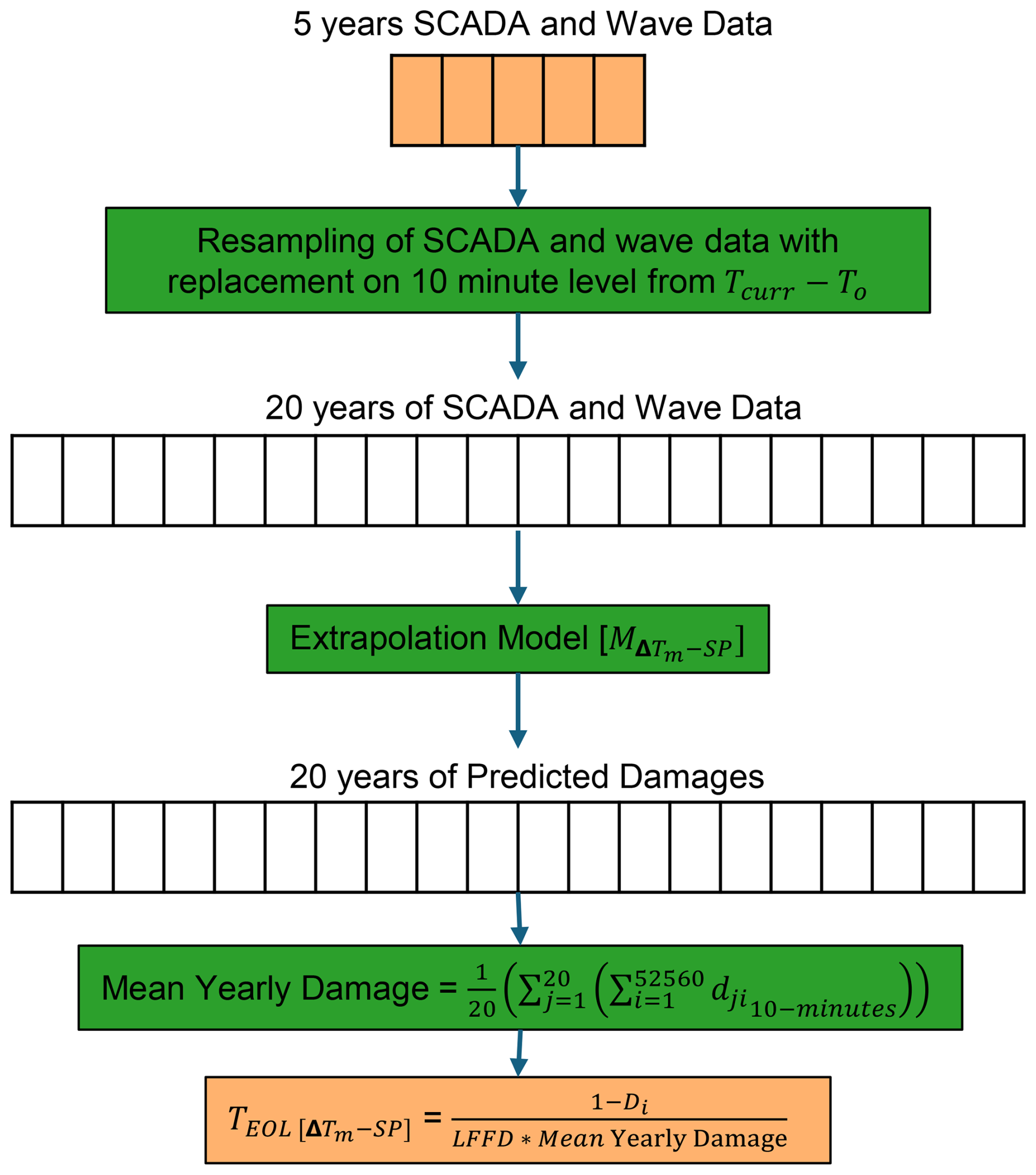
D_i is the initial damage including but not limited to pile driving damage, transportation damage, fatigue damage of the monopile foundations before start of normal operation, before turbine mounting, and powering. In this study, D_i is considered as zero as it does not affect the model comparison. In line with findings in Sadeghi et al. (2023a), a low-frequency fatigue factor LFFD_factor can be included to account for long-term cycles, which do not close within the default 10 min window. However, for simplicity, a LFFD_factor=1 is used.

5 Results

This section presents a comparative evaluation of the binning approach with varying dimensionality and random forest models across different target variables, namely single-sensor, FA, and SS damage. The predicted fatigue life for single sensor, and FA is normalized between 0.1 and 1 using Eq. (9). The scaling of SS fatigue lifetimes is done with the same scale as of FA fatigue life to retain their relative magnitudes for comparison.

$$\begin{array}{}\text{(9)}& \begin{array}{rl}{\overline{T}}_{\mathrm{EOL}}& =\left({\displaystyle \frac{T_{\mathrm{EOL}}-T_{\mathrm{EOL},min}}{T_{\mathrm{EOL},max}-T_{\mathrm{EOL},min}}}\right)\times ({\mathrm{Scale}}_{max}-{\mathrm{Scale}}_{min})\\ & +{\mathrm{Scale}}_{min},\end{array}\end{array}$$

where:

• T_EOL is the predicted fatigue life,

• ${\overline{T}}_{\mathrm{EOL}}$ is the scaled fatigue life,

• $T_{\mathrm{EOL},min}$ and $T_{\mathrm{EOL},max}$ are the minimum and maximum predicted fatigue life values obtained from all extrapolation approaches, across all dataset sizes and randomly selected start points,

• ${\text{Scale}}_{min}=\mathrm{0.1}$ and ${\text{Scale}}_{max}=\mathrm{1}$ define the target range for scaled fatigue life, suitable for plotting on the log axis.

5.1 Feature selection

Feature selection was initially performed using a filter-based method that identifies the top five features for each target variable. These selected features are summarized in Table 3. The numbers in Table 3 refer to the relative importance of the selected features, with 1 being most important feature.

For the 3 MW OWT, the results suggest a dominant influence of SCADA parameters across most target variables, with the exception of SS direction, which shows a dependency on mean wave height. In contrast, the 9 MW OWT displays a greater sensitivity to wave-related parameters across all target variables, reflecting the increased susceptibility of larger monopile structures to wave-induced effects, as already mentioned by Velarde et al. (2020); Wu et al. (2025). Notably, the SS direction for the 9 MW OWT incorporates all wave parameters except low-frequency wave direction. Although wind speed and turbulence intensity are commonly used for fatigue estimation (as studied by Noppe et al. (2020) on 2 MW OWT), our feature selection approach identifies variables that provide the greatest incremental predictive value for each target. Turbulence intensity is selected for most targets, and wind speed is included in all binning strategies (except for side–side direction of 9 MW OWT), ensuring that standard fatigue predictors are considered alongside additional influential features. Some of the selected features exhibit correlations. Random forest feature importance evaluates each variable's contribution to reducing node impurity across all trees, so correlated variables can still be selected if they provide incremental predictive information (Breiman, 2001). The top five features are thus those with the highest combined predictive relevance, and their selection reflects the overall importance rather than strict independence. Future work could explore dimensionality reduction methods to explicitly account for feature correlation.

Table 3 Overview of selected features for different target variable for 3 and 9 MW OWT.

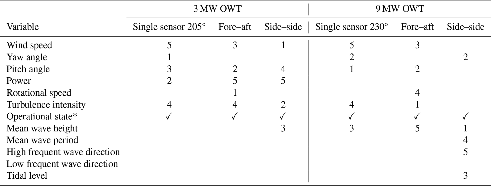
* Operational state is deliberately included in all models (a 5D model contains five EOC parameters and the turbine operational state).

In addition to the filter-based approach, RFECV was applied both globally, RFECV-Global, and separately within each turbine operational state, RFECV-Statewise. The results of these RFECV-based feature selection strategies are provided in Appendix B.

5.2 Single sensor

The fatigue damage predictions from both binning and RF models vary depending on the size of the monitoring dataset and the starting point of the data used for training. Figure 6 presents a comparison of fatigue life predictions obtained using binning (from 1D to 5D) and a 5D RF model for a 3 MW OWT.

The mean fatigue life T_EOL, denoted by the dotted gray line in Fig. 6, represents the true value of fatigue life calculated using actual measurement data. The 25th–75th percentile between the dotted orange lines is calculated by resampling the full monitoring period with replacement to synthetically generate 100 years of data. Fatigue life is then calculated for each synthetic year to get a distribution, with mean and percentiles plotted in Fig. 6. The uncertainty bounds shown in Fig. 6 represent the variability in fatigue life estimates obtained from linear extrapolation (0D binning) across multiple individual 1-year periods, rather than uncertainty across multiple 20-year spans. When multiple synthetic 20-year periods are generated, the resulting fatigue life estimates show minimal spread and converge to the mean fatigue life T_EOL line in Fig. 6.

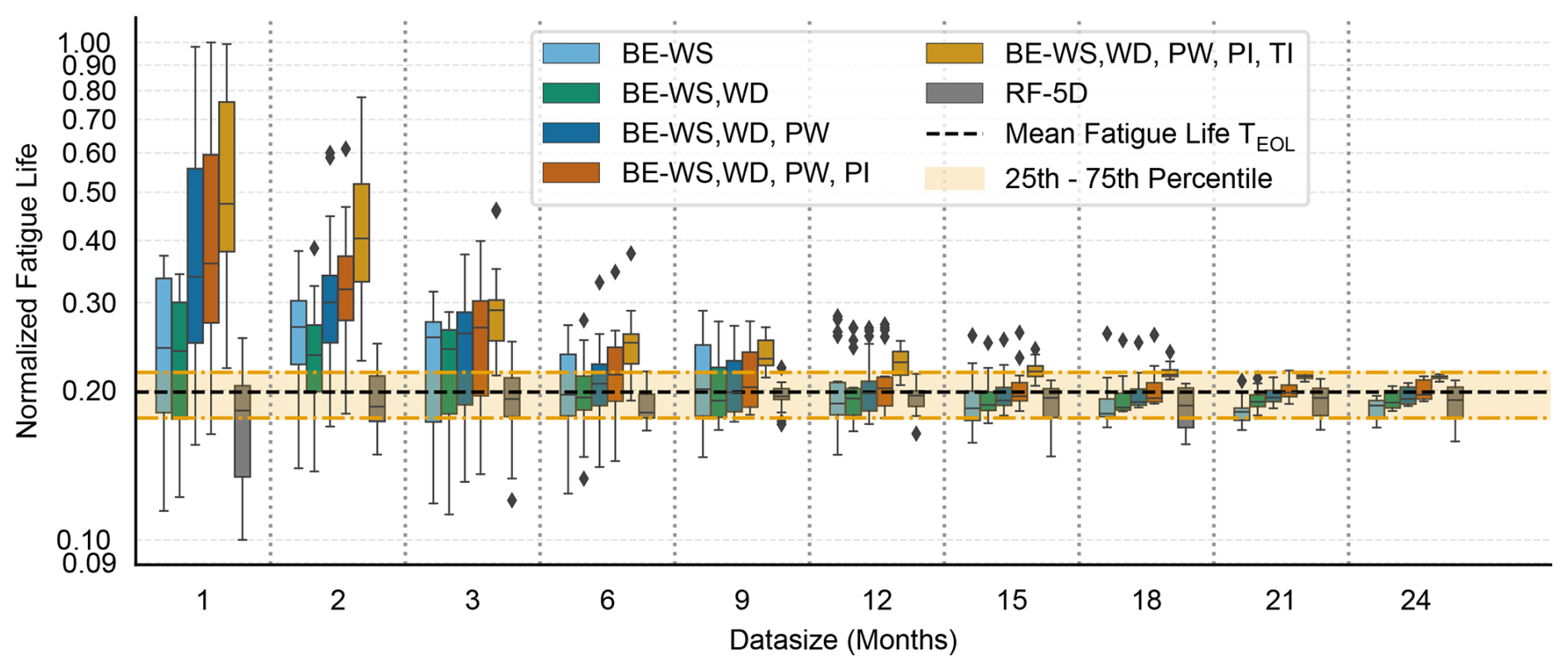
Figure 6 Comparison of binning (1D to 5D) and 5D random forest model for a 3 MW OWT at 205° single sensor.

Across all extrapolation models, a general reduction in prediction scatter is observed as the monitoring period increases, confirming the conclusions of Pacheco et al. (2023), who stated that the uncertainties in extrapolations decrease with increasing monitoring period. Notably, the prediction variability in binning approaches decreases with higher binning dimensions (e.g., from 1D to 5D). However, higher-dimensional binning tends to over-predict fatigue life, primarily due to the presence of empty bins. This sensitivity to the bin-filling strategy highlights a limitation of binning with limited data availability.

In contrast, the RF models consistently show lower scatter in predictions for smaller data sizes of 6–9 months. As data availability increases, predictions from all models begin to converge. Higher-dimensional binning, particularly 5D binning, provides consistently lower scatter in predictions from 9 months onwards, but the mean values of predictions are shifted because of unoptimized bin sizing and bin-filling strategy. The RF-5D model shows higher uncertainty and is outperformed by the binning approaches for data sizes greater than 18 months.

Figure 7 shows similar trends for the 9 MW OWT. Higher-dimensional binning again suffers from the presence of empty bins and heightened sensitivity to the bin-filling strategy, especially at smaller data sizes. The RF model demonstrates superior performance with significantly lower scatter in predictions for data sizes up to 9 months. While the difference in prediction variability between RF and binning models diminishes for larger data sizes of 18–21 months, the higher-dimensional binning methods still tend to overestimate fatigue life.

A comparison of various RF model configurations (including feature sets selected using RFECV on global data), RFECV applied separately to each operational state, and models trained using all available features is provided in Figs. C1 and C2 in Appendix C for both 3 and 9 MW OWTs. The results suggest that using statewise RFECV and individual models per operational state slightly reduces prediction scatter but introduces additional model complexity.

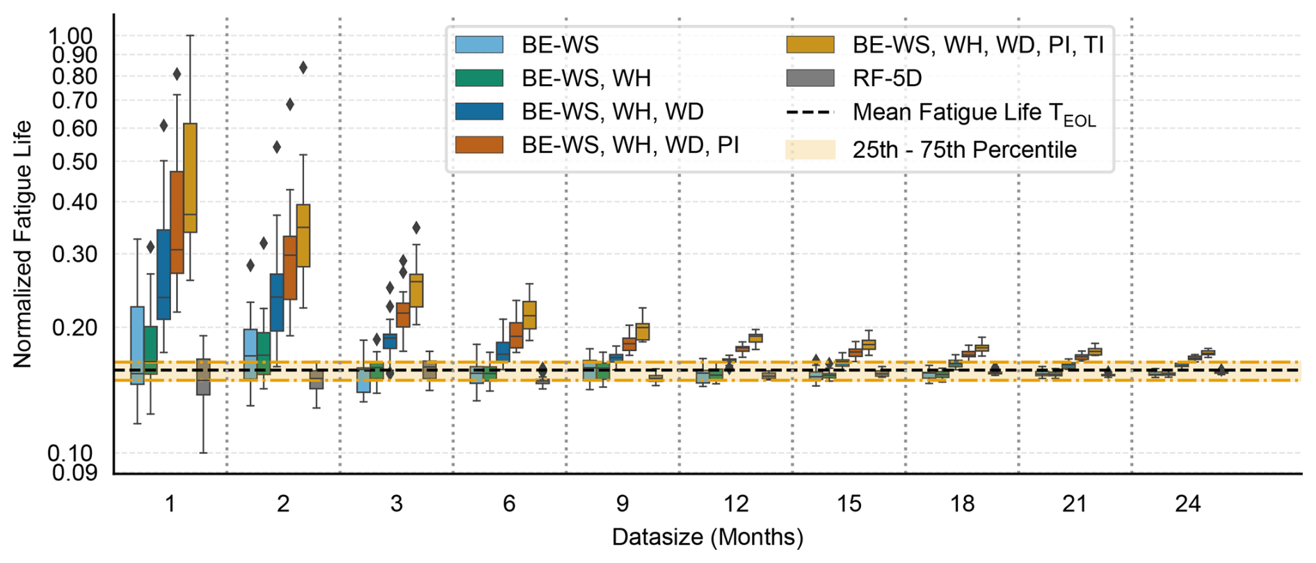
Figure 7 Comparison of binning (1D to 5D) and 5D random forest model for a 9 MW OWT at 230° single sensor.

Figure 8 illustrates the variability in predicted damage across different data sizes and starting points, binned by wind speed intervals, for 1D binning and RF models applied to a 3 MW OWT. As shown in Fig. 8, the mean predicted damage stabilizes after approximately 9–12 months of monitoring data for both the binning and RF models. However, the interquartile range (IQR), representing the spread in predictions, is consistently narrower and converges more rapidly for the RF model, indicating greater robustness to variability in the starting point. As shown in Fig. 8 (right), the IQR in the wind speed bin (21.0, 22.0) is consistently higher for the RF model than for the binning approach once more than 15 months of data are available. This increased scatter reflects the limited data availability in high-wind conditions. Consequently, for data sizes beyond approximately 15 months, the RF-5D model is outperformed by the binning-based approach, consistent with the trends observed in Fig. 6.

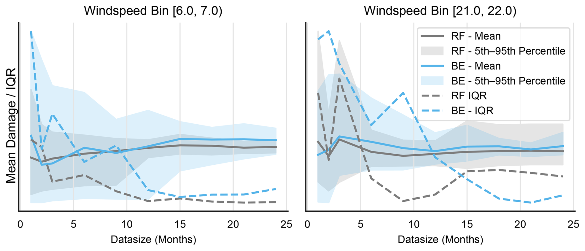
Figure 8 Mean and IQR of predicted damages using 1D binning and the 5D-RF model in wind speed bin of (6.0,7.0) (left) and (21.0,22.0) (right) for a 3 MW OWT single sensor.

Similar trends are observed in the damage predictions for the 9 MW OWT, as illustrated in Fig. 9. For the wind speed bin (7.0, 8.0), the IQR of the RF model predictions converges after approximately 9 months of data. In contrast, the IQR for the binning approach continues to decrease gradually with increasing data size, indicating a slower convergence. As shown in Fig. 9 (right), the IQR in the wind speed bin (25.0, 26.0) fluctuates between the RF-5D model and the binning approach across different data sizes. For 6, 12, and 18 months of data, the binning IQR is lower, whereas for 9 and 15 months, the RF-5D model exhibits slightly lower variability. These minor shifts arise from the very limited data available in this high-wind-speed bin, where low occurrence probability causes this apparent variability.

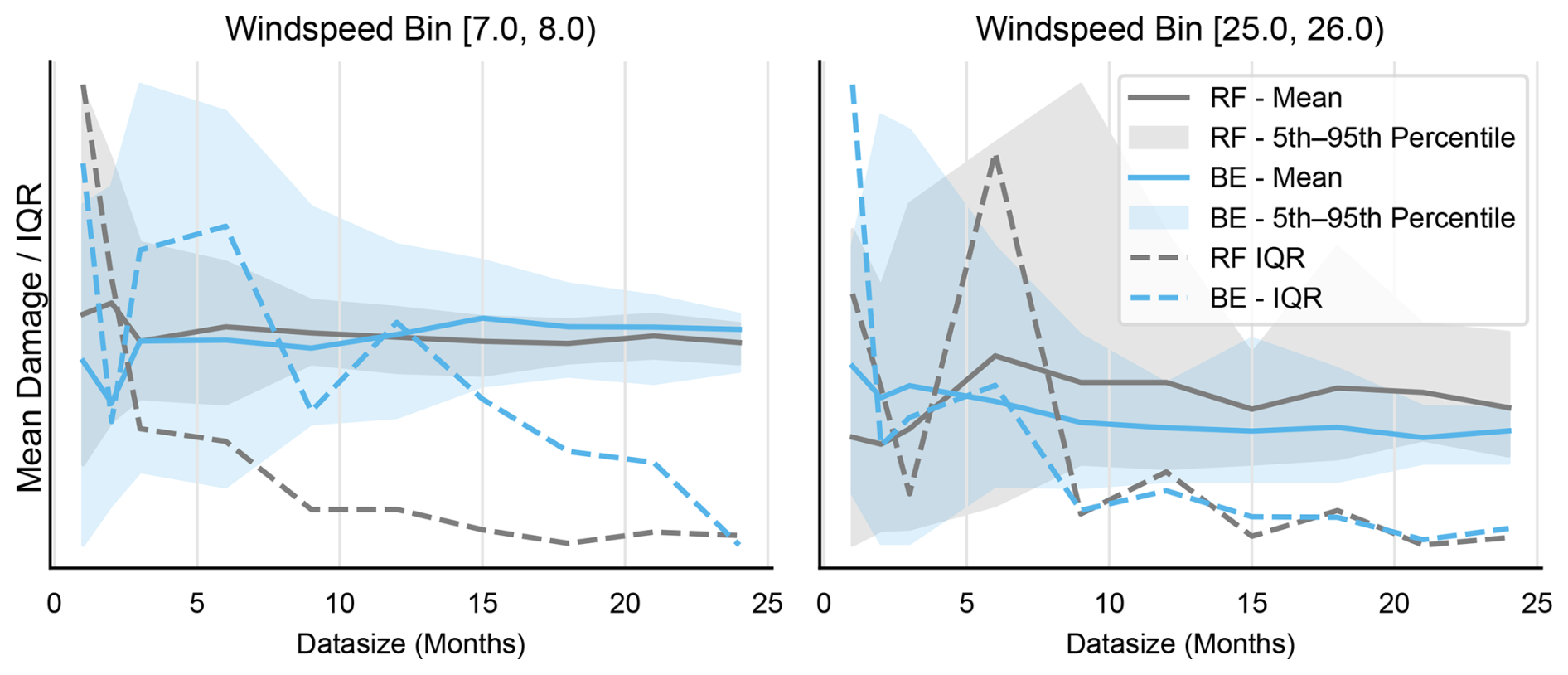
Figure 9 Mean and IQR of predicted damages using 1D binning and the 5D-RF model in the wind speed bin of (7.0,8.0) (left) and (25.0,26.0) (right) for a 9 MW OWT single sensor.

5.3 Fore–aft direction

Figure 10 presents the comparison of fatigue life predictions in the FA direction for the 3 MW OWT. The RF models exhibit a relatively constant scatter in predictions beyond 9 months of training data. For smaller data sizes of 6–9 months, RF models outperform binning methods showing lower scatter. However, for larger data sizes of greater than 12 months, higher-dimensional binning models, particularly 2D and 3D, show reduced scatter compared to RF models, indicating improved performance in fatigue life estimation.

The variability in RF predictions is further minimized by incorporating additional features, either through RFECV or by training separate RF models for each turbine operational state. The results for these alternative RF configurations are provided in Figs. C3 and C4 in Appendix C.

A similar comparison for the 9 MW OWT is illustrated in Fig. 11. In this case, RF models demonstrate superior performance at smaller data sizes, while all extrapolation methods converge to similar prediction accuracy as the data size increases. Looking at 3 months' predictions in Fig. 11, it can be noted that the predictions even for 4D binning are almost within the target region, showing lesser influence of empty bins for the 9 MW OWT in the FA direction, except in the case of 5D binning, which tends to overestimate fatigue life even when larger data sizes are used.

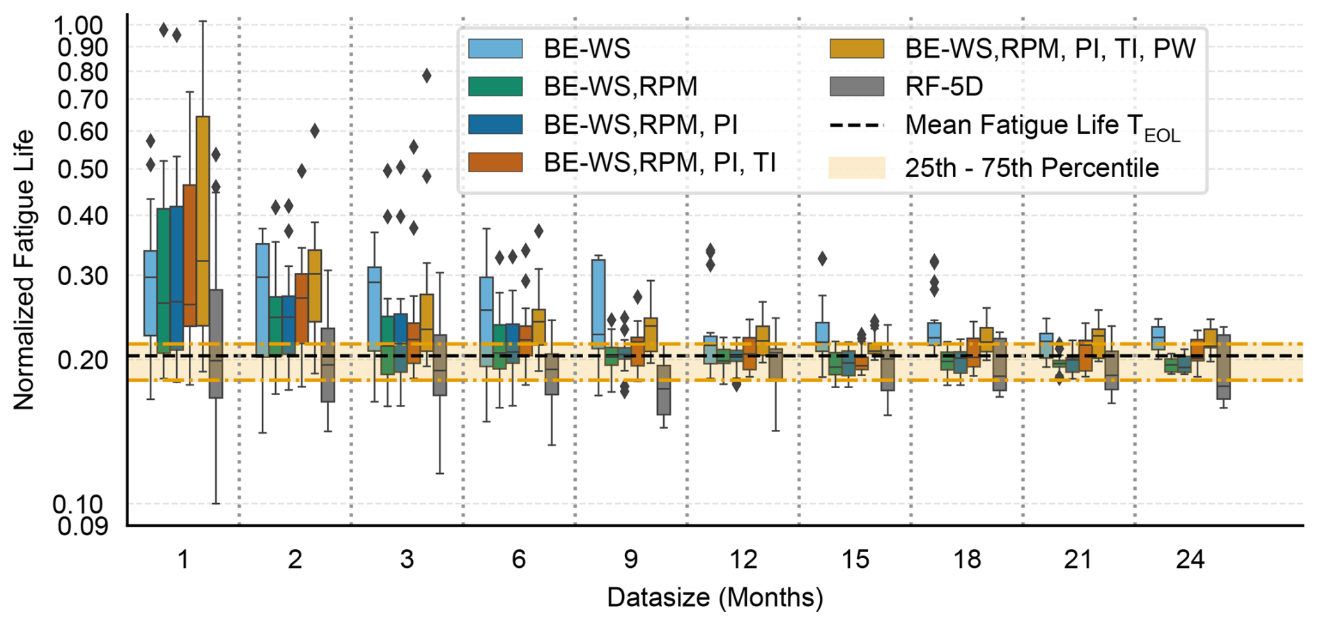
Figure 10 Comparison of binning (1D to 5D) and the 5D random forest model for a 3 MW OWT in the fore–aft direction.

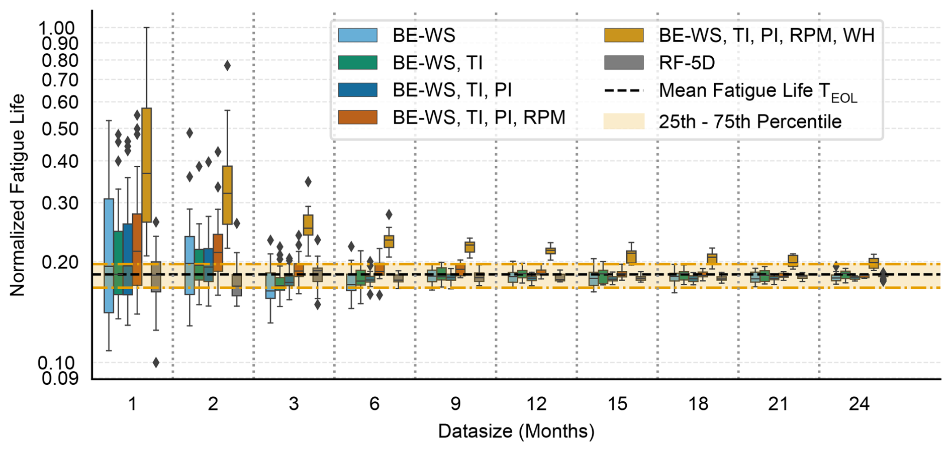
Figure 11 Comparison of binning (1D to 5D) and the 5D random forest model for a 9 MW OWT in the fore–aft direction.

5.4 Side–side direction

Figure 12 illustrates the trends in fatigue life predictions for the SS direction in the 3 MW OWT. Similar to the single sensor and FA direction cases, RF models exhibit reduced scatter at smaller data sizes of 6–9 months, and all models – including binning and RF – converge to comparable performance as the data size increases.

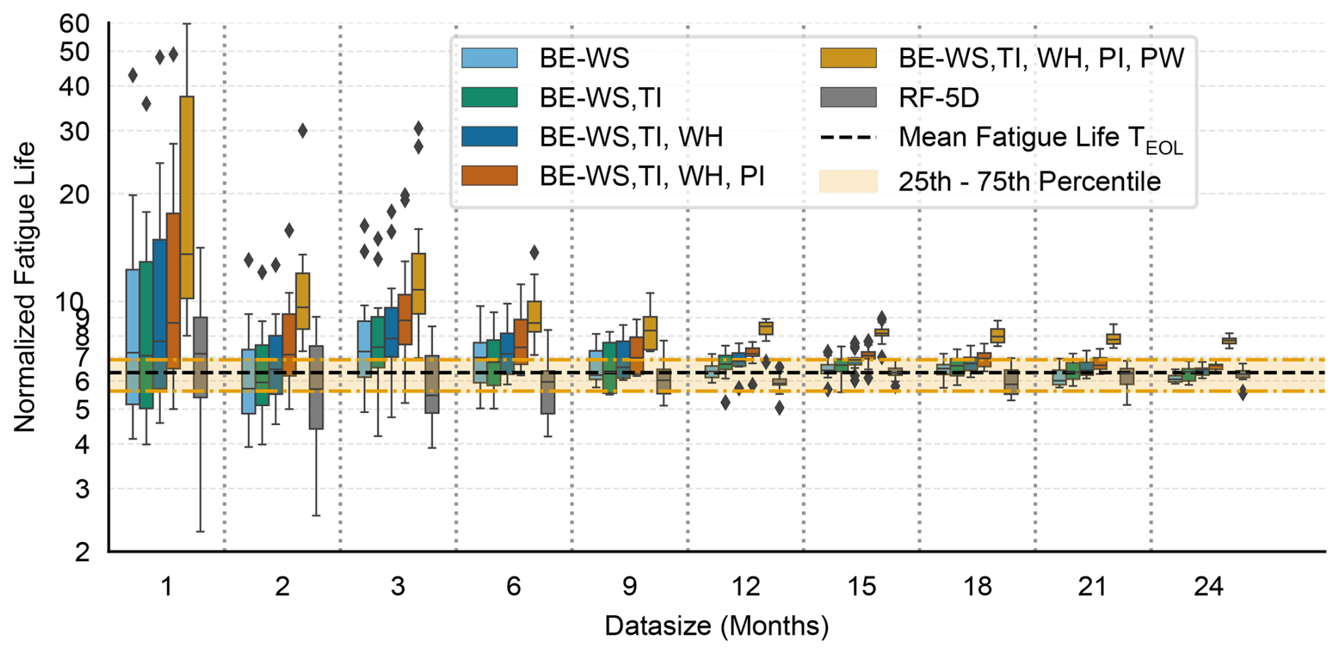
Figure 12 Comparison of binning (1D to 5D) and the 5D random forest model for a 3 MW OWT in the side–side direction.

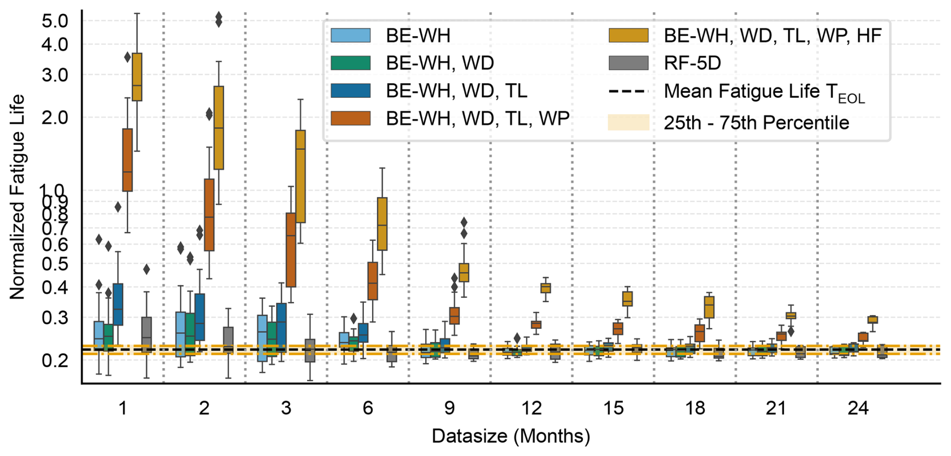
Figure 13 Comparison of binning (1D to 5D) and the 5D random forest model for a 9 MW OWT in the side–side direction.

For the 9 MW OWT, SS direction predictions show noticeable differences across models, as depicted in Fig. 13. Higher-dimensional binning approaches struggle to provide reliable predictions due to the increased sensitivity to empty bins and data sparsity. In contrast, both lower dimensional binning (1D and 2D) and RF models show consistent and comparable performance, particularly for data sizes greater than 6 months.

Notably, no significant improvement in SS direction predictions was observed through the inclusion of additional features, nor by employing RFECV or statewise RF modeling strategies, as summarized in Figs. C5 and C6 in Appendix C.

5.5 Prediction performance for different target parameters

The percentage errors over lifetime are defined as given in Eq. (10), where T_EOL, mean is the mean fatigue life calculated using actual measurement data, as described in Sect. 5.2, and T_EOL is the predicted values of fatigue life.

$$\begin{array}{}\text{(10)}& \mathrm{\text{Percentage error over lifetime}}=\left({\displaystyle \frac{T_{\mathrm{EOL}}-T_{\mathrm{EOL},\mathrm{mean}}}{T_{\mathrm{EOL},\mathrm{mean}}}}\right)\times \mathrm{100}\end{array}$$

The percentage errors over lifetime in fatigue life predictions for different target variables – FA, SS and single sensor – associated with varying training data sizes and starting points, are presented in Fig. 14 for the 3 MW OWT. For both FA and single-sensor targets, the 10th–90th percentile of the prediction errors stabilizes after approximately 9 months of training data. For the SS direction, the 10th–90th percentile of the prediction errors shows a notably low value at 12 months. The SS prediction errors stabilize after approximately 9 months of data size, assuming that the narrow percentile at 12 months is a statistical outlier. With 12 months of data, the FA direction yields prediction errors in the range of $[-\mathrm{22}\mathit{\%},+\mathrm{8}\mathit{\%}]$, while single-sensor predictions remain within a narrower error margin of approximately ±5 %. SS predictions at 12 months show improved accuracy with errors in the range of $[-\mathrm{8}\mathit{\%},\mathrm{0}\mathit{\%}]$, but the error increases to $[-\mathrm{21}\mathit{\%},+\mathrm{7}\mathit{\%}]$ at 15 months, before decreasing again with larger data sizes.

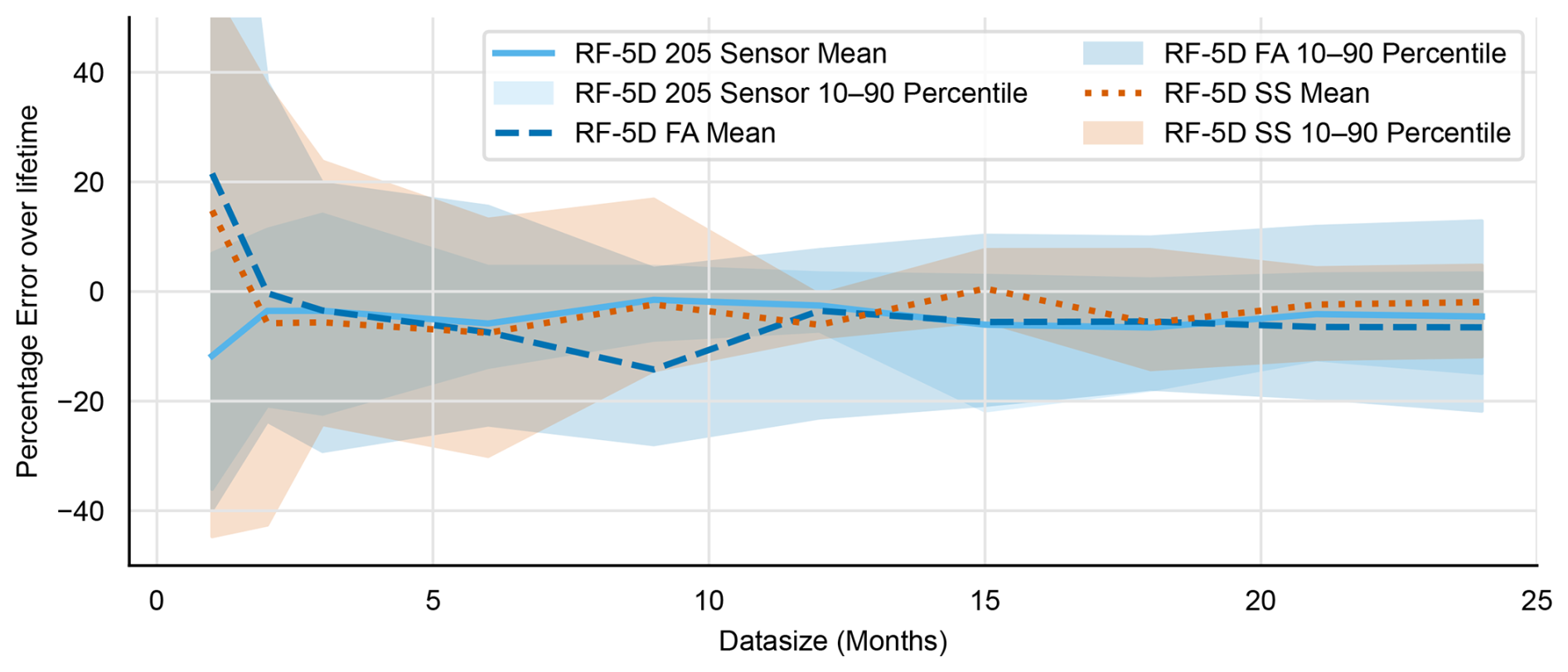
Figure 14 Percentage errors in lifetime estimation for random forest models with single sensor, and FA and SS directions for 3 MW OWT.

Figure 15 shows a similar trend for the 9 MW OWT, where error convergence is observed for all three directions: single sensor, FA, and SS. The overall prediction errors for the 9 MW OWT are lower compared to the 3 MW turbine. Specifically, using 12 months of training data, the RF model predicts lifetime errors for the single-sensor target within $[-\mathrm{10}\mathit{\%},-\mathrm{2}\mathit{\%}]$, for the FA direction within $[-\mathrm{7}\mathit{\%},+\mathrm{2}\mathit{\%}]$, and for the SS direction within approximately ±18 %.

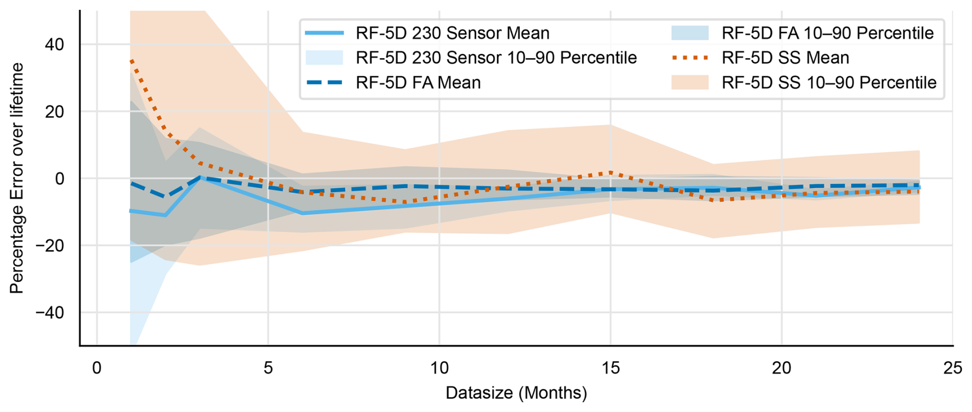
Figure 15 Percentage errors in lifetime estimation for random forest models with single sensor, and FA and SS directions for 9 MW OWT.

6 Discussions

The features selected through the filter-based feature selection method highlight the greater importance of wave parameters for SS direction in both 3 and 9 MW OWTs. Furthermore, the larger 9 MW turbine appears more sensitive to wave-induced fatigue loading compared to the smaller 3 MW turbine.

Analysis of the variation in mean damage values across different wind speed bins for the 3 and 9 MW turbines with increasing data sizes indicates that predictions converge after approximately 9–12 months of monitoring data. Additionally, the scatter in predictions is significantly lower for RF models than for binning-based extrapolation for smaller data sizes. For larger data sizes, for example, in the 3 MW OWT case beyond 18 months, the RF models show comparable or higher scatter and are outperformed by binning-based extrapolation models. A strain monitoring period of 9–10 months is also recommended in the literature (Hübler et al., 2018; Hübler and Rolfes, 2022) to capture critical fatigue-inducing events, such as high wind speeds and seasonal variability, provided that no significant changes occur in the turbine or its EOCs during this time.

The availability of long-term monitoring data enables the investigation of how the randomly varying starting point of the monitoring period influences the variability in fatigue life estimates. A comprehensive comparison between binning and RF model predictions shows that when accurate fatigue life estimates are required in shorter time frames of 6–9 months, RF models yield lower statistical uncertainty than binning approaches. RF models are more effective at capturing the nonlinear relationships between SCADA, and wave parameters and fatigue damage, particularly when limited data are available. For longer data durations, greater than 15 months, both RF and binning methods provide comparable fatigue life predictions. When long-term measurement data are available, binning extrapolation should be preferred as they are more transparent, provide easy control of conservativeness using alternate bin filling strategies, and have a stronger link with design as indicated by their similarity to design load cases (DLCs) (International Electrotechnical Commission, 2019; Freudenreich and Argyriadis, 2007).

Increased dimensionality in binning, especially 4D and 5D, results in reduced performance compared to lower-dimensional – 1D and 2D – binning. This is primarily due to the treatment of empty bins. Alternative strategies for empty bin filling, such as using the 90th percentile, the highest neighboring value, or interpolation methods based on surface fitting (Pacheco et al., 2023; Noppe et al., 2020; Hübler and Rolfes, 2022), could enhance the accuracy of high-dimensional binning. In this study, bin sizes are not explicitly optimized. Future work may involve optimizing bin sizes for different data sizes, similar to hyperparameter tuning in RF models, to further improve binning performance.

From a usability perspective, 1D and 2D binning are computationally efficient and easy to implement. However, higher-dimensional binning – 3D and above – becomes increasingly computationally expensive, especially when combined with complex empty-bin-filling strategies. On the other hand, RF models, while offering improved prediction accuracy, are more complex and require intensive hyperparameter tuning. More advanced RF pipelines, such as those involving different models for different operational states, can further enhance accuracy but at the cost of increased computational effort and reduced interpretability.

RF models using filter-based feature selection offer a good trade-off between complexity and predictive performance. In practical scenarios where a turbine is instrumented later in its lifetime and a fast, reliable fatigue life estimate is required, RF models can be particularly valuable.

While this study evaluates the statistical uncertainty associated with varying the start of the monitoring period, another layer of uncertainty arises when predictions are made using a fixed data size and start point, especially if the training and extrapolation data differ significantly. Both binning and RF models in this work rely on the mean damage within each bin or the mean prediction, without considering the full distribution. Such uncertainties have been explored in the context of binning by Sadeghi et al. (2024). Future work could explore the use of quantile random forests (Rouholahnejad and Gottschall, 2025) to quantify this uncertainty. Additionally, Bayesian neural networks may be employed to flag outliers in fatigue life predictions based on differences between training and extrapolation datasets. These advanced uncertainty quantification techniques are beyond the scope of this paper and are proposed as future work.

Finally, it is important to note that the findings of this study are applicable to the wind farms analyzed and, by extension, are likely relevant to the majority of farms located in the North Sea. However, in locations exhibiting differing levels of environmental variability, the applicability of these recommendations may be limited.

7 Conclusions

This study concludes that a monitoring period of 9–12 months is required to obtain reliable fatigue life estimates for OWTs, based on case studies using long-term monitoring data from both 3 and 9 MW turbines. Feature selection results further demonstrate that the relevance of input parameters depends on the target variable, i.e., single sensor, FA, or SS damage. For the larger 9 MW OWT, wave parameters appear consistently across all target variables, whereas for the smaller 3 MW turbine, only SS fatigue damage includes mean wave height as a key feature. These conclusions specifically apply to offshore wind farms analyzed in the Belgian North Sea and requires re-evaluation for locations exhibiting varying degrees of environmental variability.

Random forest models exhibit better generalization capability compared to binning-based extrapolation methods, as evidenced by their reduced sensitivity to the starting point of the monitoring period. Higher-dimensional binning of 3D and above suffers from issues with empty bins, especially when using smaller datasets. Consequently, RF models are more effective for fatigue life prediction when limited data are available, offering lower statistical uncertainty than binning methods.

The predictive advantage of RF models over binning diminishes as the monitoring period increases, beyond 12–15 months, at which point both approaches yield comparable performance. Furthermore, more complex RF models involving additional features or operational state-specific modeling offer only marginal improvements in accuracy.

Future work may enhance the accuracy of binning methods by optimizing bin sizes and systematically evaluating the effects of various empty bin-filling strategies. These improvements could help to narrow the performance gap between binning- and machine-learning-based approaches, particularly for high-dimensional binning models.

Appendix A: Effect of different bin-filling strategies using 3D binning

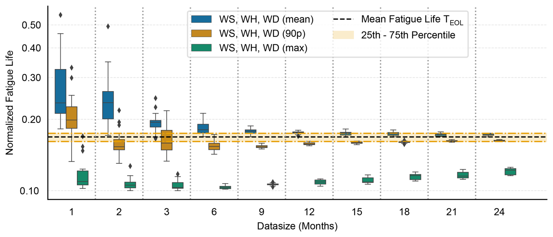
Figure A1 Effect of different bin-filling strategies on lifetime predictions using 3D binning for a 9 MW OWT at 230° single sensor.

Appendix B: Feature selection using RFECV-Global and Statewise

B1 RFECV-Global features

RFECV was applied to 12 months of data to identify the most relevant features for fatigue life prediction. Operational states were incorporated into the feature space using one-hot encoding. The selected features for both the 3 and 9 MW offshore wind turbines are given in Table B1.

Table B1 Selected features for different target variable for 3 and 9 MW OWT using RFECV on 12 months of data.

* Operational state is deliberately included in all models.

B2 RFECV-Statewise features

RFECV was applied to 12 months of data by first filtering the dataset into individual operational states and performing RFECV separately on each subset. The resulting RFECV-Statewise feature sets for both the 3 and 9 MW offshore wind turbines are given in Tables B2 and B3.

Table B2 Operational statewise selected features using RFECV-Statewise on 12 months of data for 3 MW.

1: nominal, 2: idling, 3: high wind, 4: transient. * Operational state is deliberately included in all models.

Table B3 Operational statewise selected features using RFECV-Statewise on 12 months of data for 9 MW.

1: nominal, 2: idling, 3: curtailed, 4: transient. * Operational state is deliberately included in all models.

Appendix C: Comparison of different RF configurations

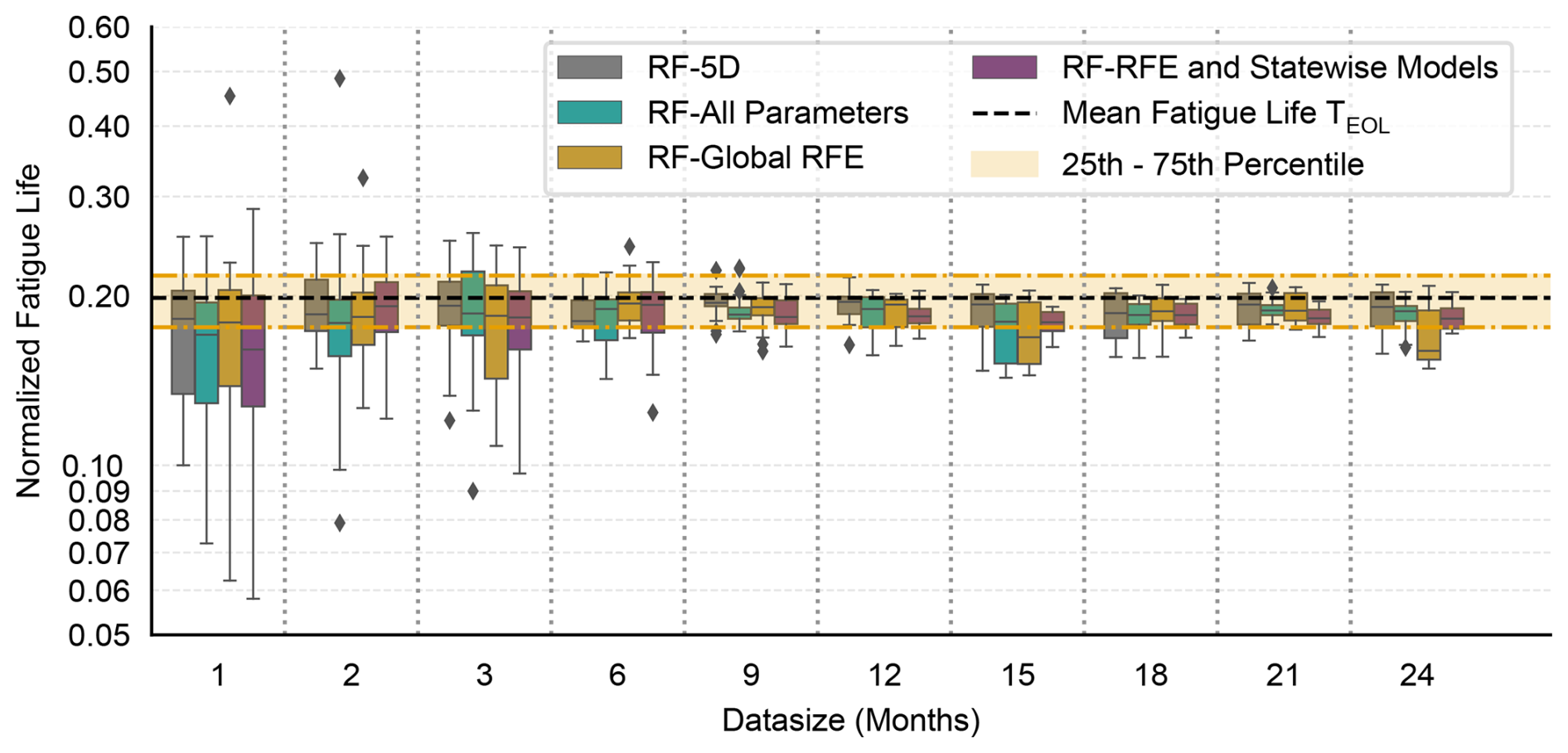
Figure C1 Comparison of different RF model configurations for a 3 MW OWT at 205° single sensor.

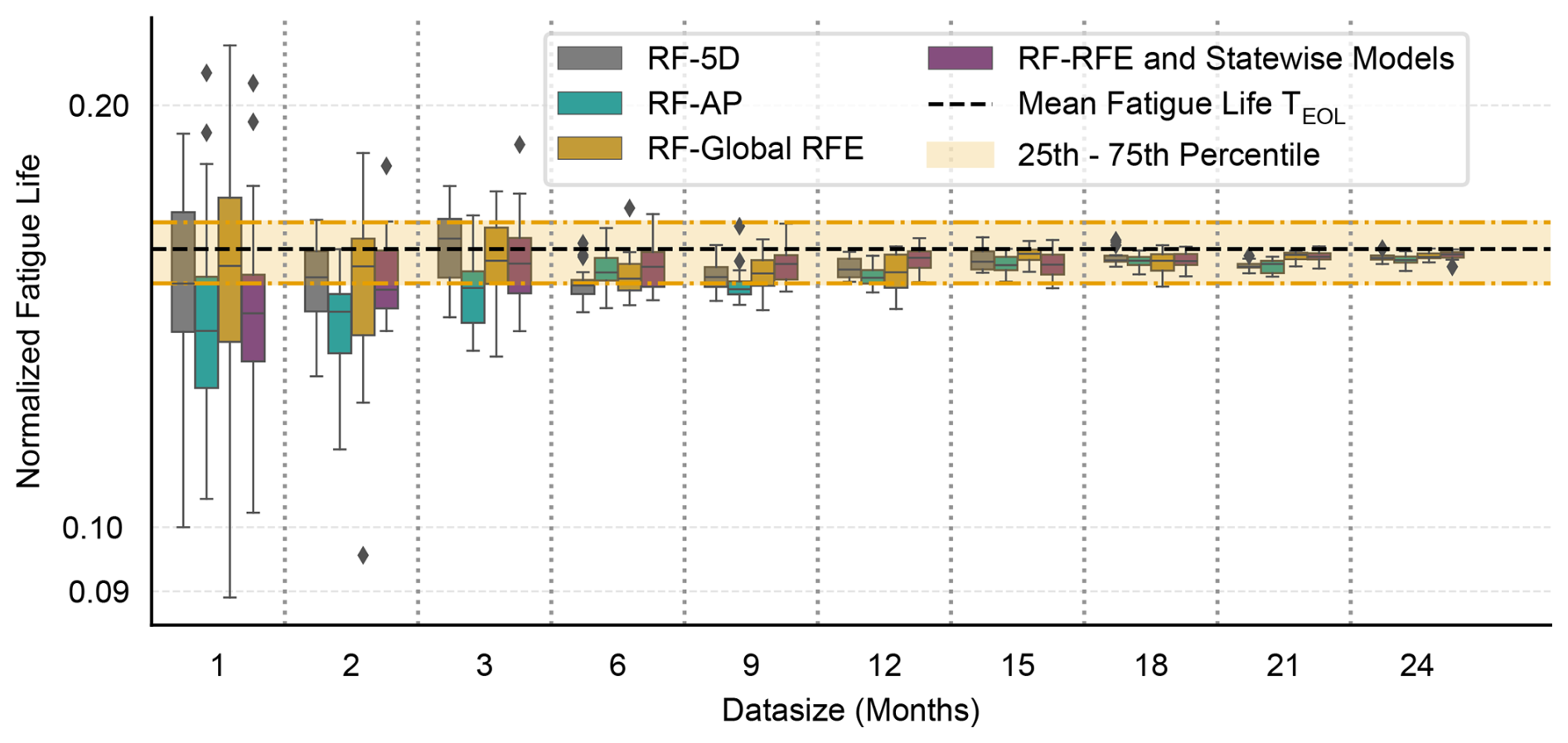
Figure C2 Comparison of different RF model configurations for a 9 MW OWT at 230° single sensor.

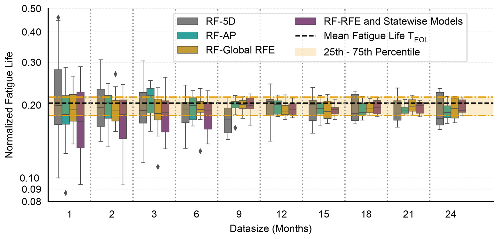
Figure C3 Comparison of different RF model configurations for a 3 MW OWT in the FA direction.

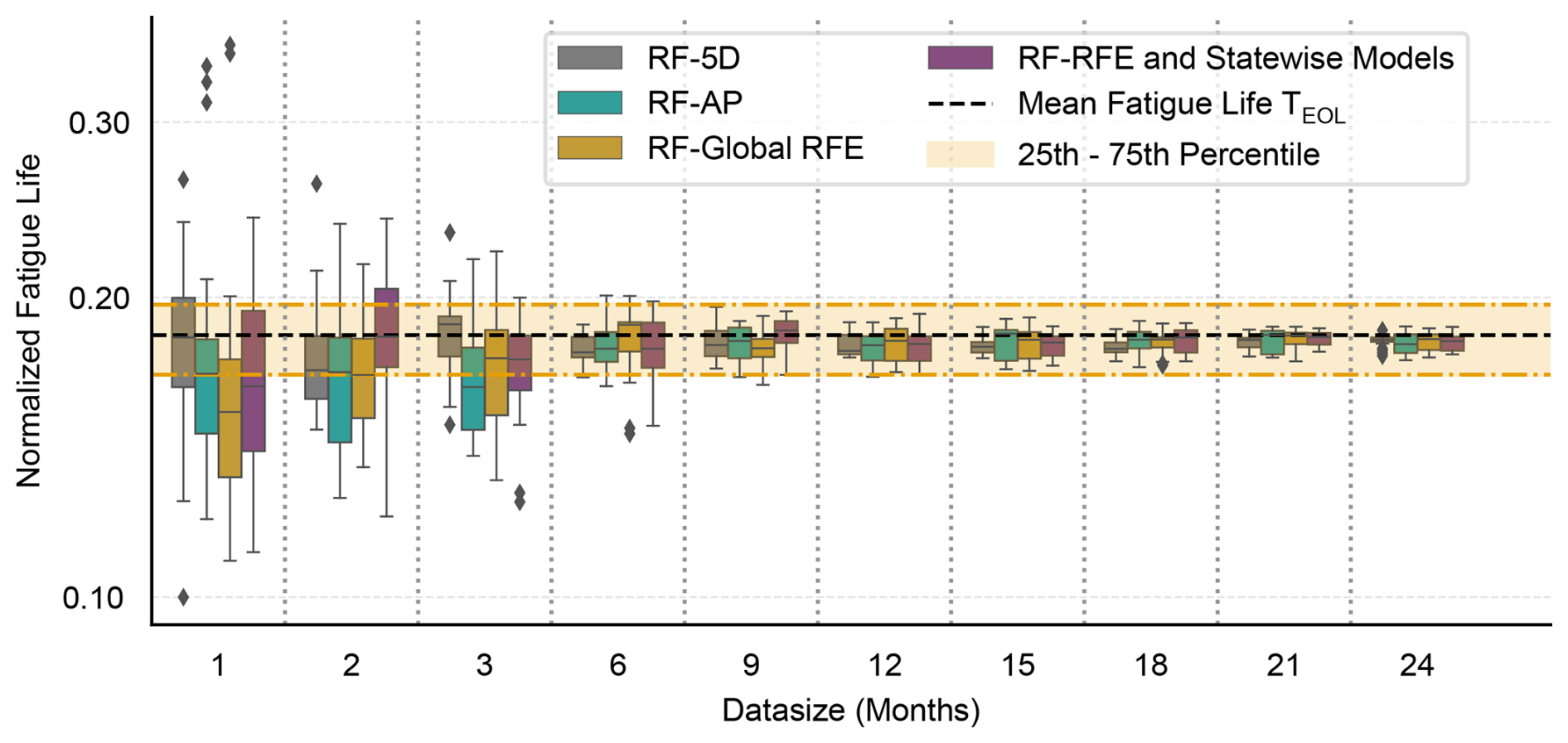
Figure C4 Comparison of different RF model configurations for a 9 MW OWT in the FA direction.

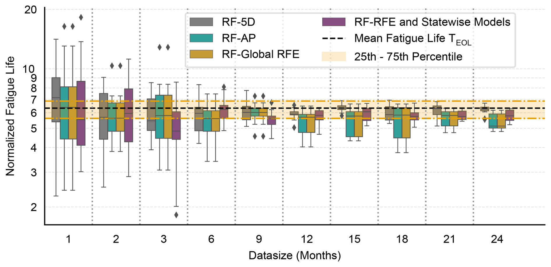
Figure C5 Comparison of different RF model configurations for a 3 MW OWT in the SS direction.

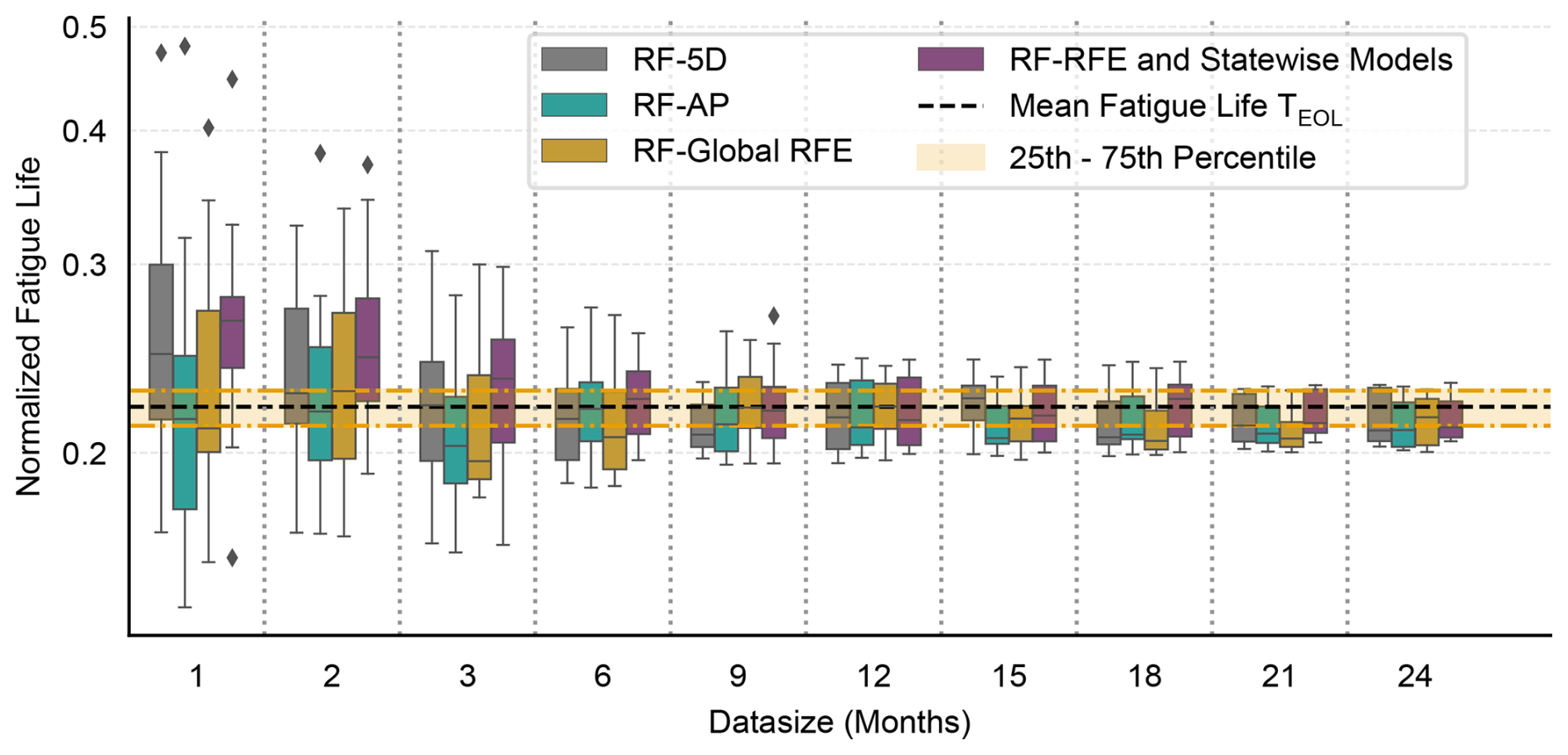
Figure C6 Comparison of different RF model configurations for a 9 MW OWT in the SS direction.

Appendix D: Bin sizes

Table D1 Bin sizes for SCADA and wave parameters.