Added value of site load measurements in probabilistic lifetime extension: a Lillgrund case study

Site-specific fatigue estimation is an essential part of wind turbine lifetime extension, with various methods depending on data availability.

The present study compares probabilistic lifetime extension assessment results for rotor blades with and without load measurements. It also addresses two key questions in such assessments: the applicability of the Frandsen model for estimating waked turbulence under complex and mixed wake conditions and the extrapolation of mid-term data over longer time periods.

The case study wind turbine is SWT-2.3-93, located at the edge of the Lillgrund wind farm, situated in the Øresund Strait between Denmark and Sweden. The turbine is extensively instrumented, with 5 years of data available from its supervisory control and data acquisition (SCADA) system.

Although the Frandsen turbulence estimates deviate in a different manner from measurements at below- and above-rated mean wind speeds, the model remains a conservative approach for fatigue load prediction and reliability.

In the current case study, the site-specific assessment using strain gauge measurements yields a 33 % higher annual fatigue reliability index after 35 years compared to a scenario based on the Frandsen estimation combined with ambient environmental data and a generic aeroelastic model. The results also demonstrate that the sensitivity of fatigue reliability to load uncertainty is negligible when load measurements are used directly but relatively high when relying on the Frandsen model in combination with a generic aeroelastic model. Overall, the high variability of the lifetime extension in different scenarios of data availability and accuracy shows the importance and added value of high-quality measurements combined with wind-farm-level SCADA and a model updated in real time (digital twins).

1 Introduction

Exposure of wind turbines to the wakes within a wind farm increases the fatigue loads they experience (Kim et al., 2015; Lee et al., 2013; Frandsen, 2007). However, the design assumptions in the IEC 61400-1 standard are often conservative enough to allow seeking an extension of the operation time even after experiencing the high fatigue loads caused by wakes in wind farms. Extending the operation time above the design service life (typically 20–25 years), in cases where maintaining safety is possible, is environmentally beneficial and can reduce the levelized cost of energy (Dimitrov and Natarajan, 2020; Natarajan et al., 2020).

When it comes to lifetime extension of wind turbines in a wind farm, one must reassess the service lifetime by replacing the design assumptions with the conditions experienced at the site as the analytical part (DNV-ST-0262, 2016). In such reassessments, fatigue is typically the primary focus, as it represents one of the most critical time-dependent degradation mechanisms. Information about in situ lifetime can be obtained in various ways, depending on data availability. Often, the turbine model is not available and generic models are used. Some of the common scenarios under this condition include the following:

1. Often, high-quality environmental measurements at the turbine's specific location are not available, whereas freestream turbulence measurements are. In such cases, waked turbulence at each turbine location can be estimated using simplified models such as the Frandsen model (Frandsen, 2007; Frandsen and Madsen, 2003), suggested by International Electrotechnical Commission (2019) for site-suitability checks. The resulting estimates are then used to perform aeroelastic simulations with a generic turbine model, from which site-specific lifetime can be assessed.

2. In some cases, structural response measurements (e.g., load or displacement) are available for a limited duration and at specific hotspot locations. Direct use of these measurements for lifetime extension assessment is possible, but it involves challenges, such as spatial extrapolation (from one location in the structure to another) and temporal extrapolation (from one point in time to another).

3. When structural response measurements are complemented by supervisory control and data acquisition (SCADA) data and high-quality environmental measurements, a digital twin can be developed to estimate loads accurately in all components or locations within the turbine.

Often, structural response measurements collected at the site are owned by the turbine manufacturer and are not accessible to the wind farm owner or developer. Moreover, when available, such measurements are typically limited in both duration and spatial coverage. This research compares lifetime extension assessments for two scenarios, using a case study in which both scenarios can be explored. Because of the inaccuracy of the wind measurements from the anemometer – due to the location of the met mast and unavailability of the SCADA of the neighboring wind turbines – the measurements are not directly used in waked directions. Freestream measurements are used for model validation (see Appendix). In addition, the study addresses two common challenges encountered in these scenarios, as outlined below:

1. evaluating the performance of the Frandsen model, a simplified method for estimating wake-induced turbulence, in a compact wind farm layout (scenario 1)

2. developing a method for the statistical extrapolation of mid-term strain gauge data to estimate long-term fatigue loads (scenario 2).

The Frandsen model is based on simplified assumptions and carries inherent uncertainties. The uncertainty associated with fatigue load estimation using this model is discussed in a few examples by Frandsen (2007). Several limitations of the Frandsen model have also been identified. For instance, Bayo and Parro (2015) and Argyle et al. (2018) highlight issues such as the lack of a defined method for accounting for wake interactions among multiple turbines and the potential for under-conservative predictions when the wind farm significantly affects the mean wind speed. Therefore, in wind farms with compact and/or irregular layouts, verifying the Frandsen model's performance for conservative site-suitability assessments is crucial. Although prior studies have examined the model's general performance, its applicability in high-wake-interaction conditions – particularly those resulting from tight turbine spacing (e.g., less than five rotor diameters) and irregular configurations – remains unexplored. The current work compares turbulence estimates from the Frandsen model with actual measurements at the Lillgrund wind farm, as an example of compact layout, to assess the accuracy of the model under various waked flow conditions.

A challenge in scenario 2 for assessing site-specific lifetime is the limitation of available data and the need to extrapolate short-term load measurements to cover longer periods for fatigue damage estimation. Determining turbine-specific fatigue accumulation throughout the operational lifetime under such constraints remains a critical open question. This issue is particularly significant for offshore wind farms, where the high variability and scatter in environmental conditions adds to the complexity of accurate fatigue lifetime assessment. Some studies, including Amiri et al. (2019) and Ziegler and Muskulus (2016), assess lifetime extension by assuming a linear increase in fatigue damage over time. However, this approach can introduce significant errors when the available data are insufficient to accurately estimate the damage equivalent load (DEL). Although DEL is an averaged metric and therefore generally more robust to individual outliers (Mozafari et al., 2023b), it can still exhibit considerable variability depending on the length of the dataset – particularly for components with high fatigue exponents. As an example, the results of Mozafari et al. (2023a) show that the conventional approach of assuming a constant DEL – implying a linear increase in damage accumulation over time – can introduce high bias in long-term fatigue damage assessments, particularly for blades. This is due to the high fatigue exponent associated with composite materials used in blade structures.

Some studies, such as Dimitrov and Natarajan (2019) and Natarajan et al. (2020), have employed machine learning techniques and Monte Carlo simulations to generate long-term fatigue load estimates from mid-term response measurements. Other studies, including Ling et al. (2011), Hübler et al. (2018), and Natarajan (2022), have applied stochastic methods to predict long-term fatigue behavior based on shorter-term load data. Despite different statistical approaches and the guidelines given in International Electrotechnical Commission (2019), the best procedure to statistically extrapolate fatigue loads remains unclear. The current work presents a procedure capturing the multimodality of fatigue load data – as demonstrated to be effective in Mozafari et al. (2023a) – and extrapolates it over the full assessment duration.

The current study assesses the feasibility of extending the operational lifetime of the wind turbine blades by 10 years at the edge of the Lillgrund wind farm while ensuring that acceptable safety margins are maintained. In the current study, the turbulence data in a location close to the wind turbine are available and are utilized for validation purposes and to illustrate the extent of error associated with the generic model used in the study.

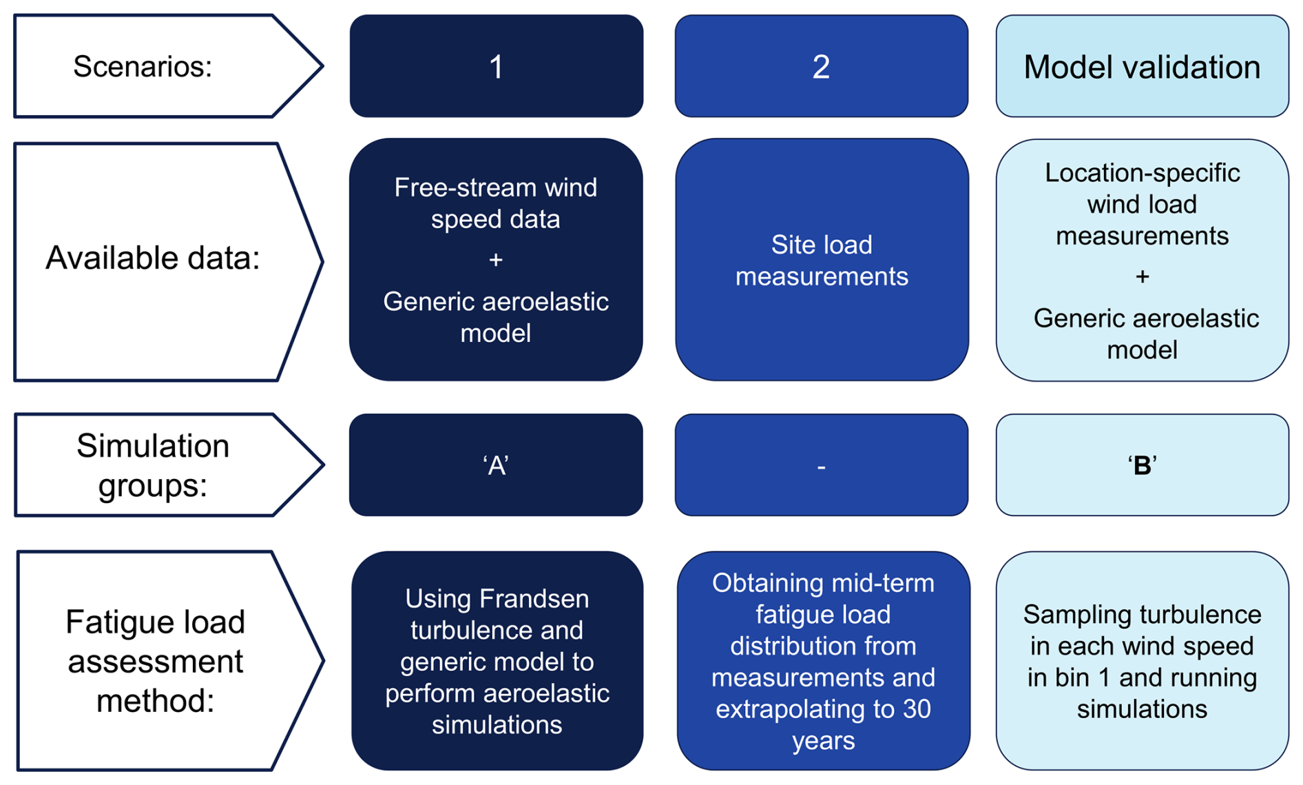
Figure 1 Overview of site-specific assessment scenarios (studied in the present work) with corresponding data availability, simulation approaches, and load estimation methods.

First, demonstrating scenario 1, using the available SCADA data and the generic model of the turbine, we evaluate the performance of the Frandsen model in conservatively estimating fatigue loads at the case study wind farm. To enable a more detailed assessment of the model's turbulence predictions, we classify and bin different wake scenarios affecting the case study wind turbine. Second, demonstrating scenario 2, we employ a gamma mixture model to represent the bi-modally distributed mid-term DEL data, derived from 10 min strain measurements at the blade root, and extrapolates them to a 30-year operational lifetime. Finally, we show the annual fatigue reliability levels of the blade in different scenarios versus design (simulated via the generic model) to highlight potential differences in the lifetime extension feasibility. In addition, the relative influence of three key factors on fatigue reliability estimation across scenarios 1 and 2 is studied: the applied loads, the material's fatigue strength, and the chosen damage accumulation rule. Different scenarios and the corresponding simulations used in the current study are shown in Fig. 1.

Awareness of the effects of different sources of uncertainty on lifetime extension assessment is valuable and can help improve the accuracy and robustness of such evaluations. The presented procedure for extrapolating fatigue loads can help stakeholders and wind farm owners obtain a more accurate assessment of fatigue damage in cases where strain gauge measurements are unavailable or only available for a limited period of the turbine's lifetime. To make the life extension results interesting for this specific example, the material properties are calibrated to achieve a target reliability index of 3.7 (International Electrotechnical Commission, 2019) after 20 years, based on the design class (as would result from applying the recommended safety factors from the standard). Thus, while the comparisons of reliability levels are valid, their absolute magnitudes are not.

In the next sections, first, we present the methods and models we use for modeling and reliability assessment (Sect. 2). Then we present the results and corresponding discussions of the Frandsen performance check and lifetime extension assessments in Sect. 3. Finally, in Sect. 4, we present the conclusions of both studies and suggestions for future work. The main codes used in the study can be accessed through Mozafari (2026).

2 Methodology

First, we introduce the case study wind turbine and the corresponding wind farm in Sect. 2.1 and 2.2, respectively. Then, in Sect. 2.3, we present the setup and features of the aeroelastic simulations and site load measurements. In addition, we introduce the methods we use for assessing and filtering data for the current study. Finally, in Sect. 2.4, we introduce the mathematical formulas and the procedures we use for post-processing the simulation results and load measurements.

2.1 The case study wind turbine

The wind turbine under study in the current research is SWT-2.3-93, manufactured by Siemens Energy. The turbine has a 92.6 m rotor diameter, a hub height of 65 m, and a rated power of 2.3 MW. The cut-in and cut-out mean wind speeds are 3 and 25 m s⁻¹, respectively, reaching the nominal power at approximately 12–13 m s⁻¹. The turbine belongs to class 1A based on the IEC 61400-1 standard's classification. A generic model of this turbine is used for the assessments (Dahlberg , 2009).

2.2 The case study wind farm

The strain gauge and environmental measurements belong to one of the turbines at the edge of the Lillgrund offshore wind farm. Lillgrund wind farm is located about 10 km off the coast of Sweden in the Öresund region and consists of 48 Siemens SWT-2.3 93 wind turbines (total capacity of 110 MW). The turbines are arranged as shown in Fig. 2. The circles in Fig. 2 represent different turbines, and the red circle is the case study wind turbine, denoted as C08 (row c and column 8). We bin the wind directions around the case study wind turbine to roughly distinguish between different wake conditions. The binning facilitates assessing the performance of the Frandsen model and IEC NTM assumptions in characterizing turbulence in different wake scenarios. The dashed lines in Fig. 2 show the bins. For the rest of the study, we refer to the wind direction bins as “wind bins” for simplicity.

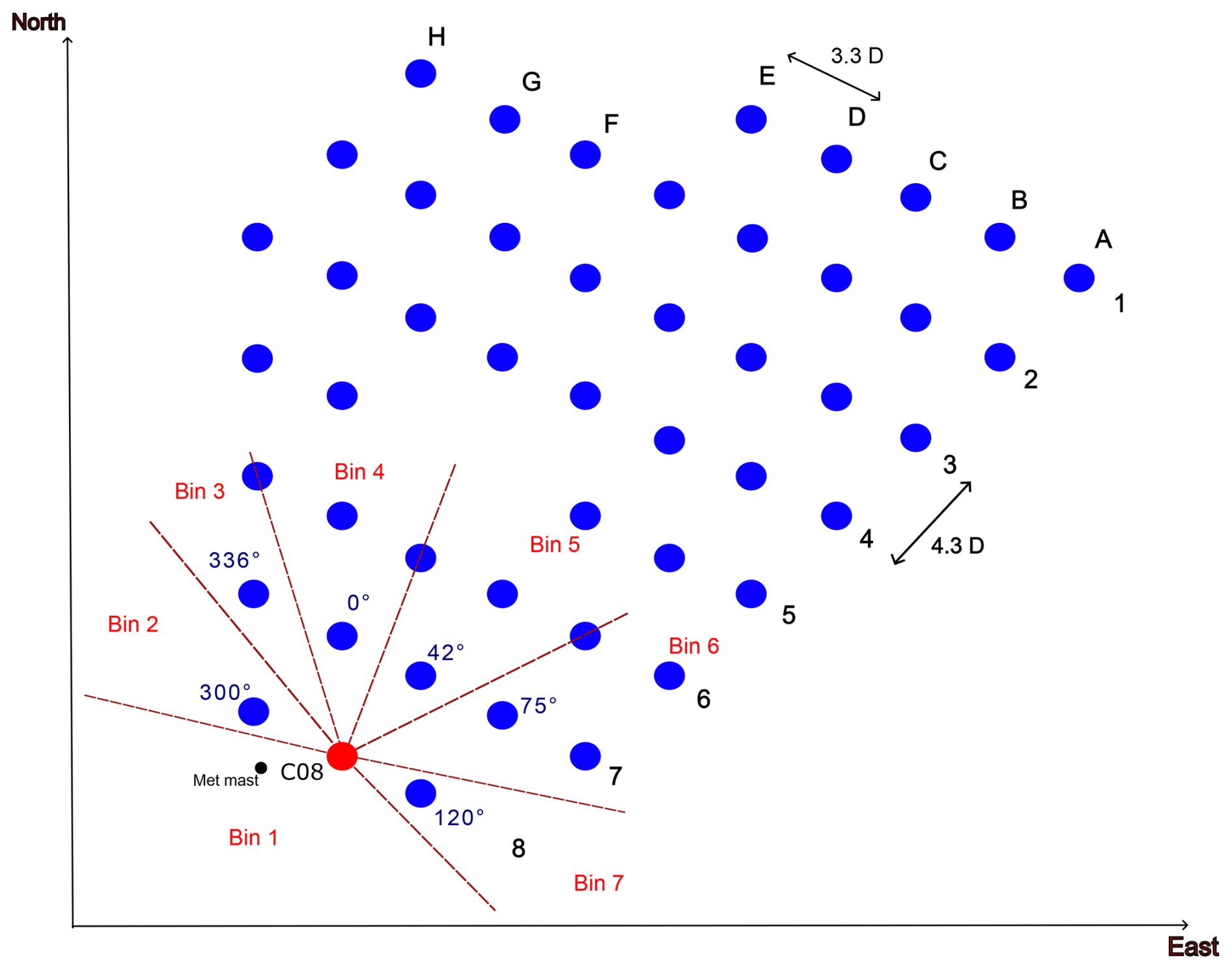
Figure 2 Arrangement of the wind turbines in the Lillgrund wind farm and the wind direction bins around the turbine C08 used in the current study.

As illustrated in Fig. 2, wind bin 1 accounts for non-waked conditions. In wind bins 2, 3, and 7, the stream mainly passes by a single turbine, with bin 3 representing a relatively long distance between the turbine generating the wake and the C08 wind turbine. Wind bin 5 is an intense condition, with the case study turbine being very deep in the row and a very short distance between the closest wind turbine (4.3 times the rotor diameter). Bin 4 is a similar arrangement of a single row with a relatively long distance, and bin 6 is a mixed waked flow condition. One should note that the binning and the corresponding conditions described are qualitative and are only used for general comparison.

2.3 Measurement data and aeroelastic simulations

In the present study, we use SCADA and 10 min DEL evaluations extracted from a strain gauge installed at the blade root. The data represent long-duration measurements over a span of 5 years in the Lillgrund wind farm. We also perform aeroelastic simulations in HAWC2 software (Larsen and Hansen, 2007). In the following, first, we introduce the available measurement data (from the strain gauge and SCADA). Then, we present the specifications of the three groups of aeroelastic simulations used.

2.3.1 Measurement data

The available data include strain gauge measurements and SCADA records, comprising wind speed, wind direction, power output, and rotor speed. The mean and standard deviation of wind are derived based on an anemometer mounted on a meteorological mast located in close proximity to the case study wind turbine (black dot in Fig. 2). The meteorological mast is placed on a pole on top of the tower at a height of 65 m (for more information, see Bergström, 2009). In addition, the strain gauge is installed 1.5 m away from the blade root. All data are measured in time intervals of 10 min during the years 2008 to 2012. The strain gauge measurements are transformed into 10 min DELs using the Palmgren–Miner approach, considering a Wöhler exponent equal to 10 for the composite structure of the blade. The measurement campaign has been running for over 5 years but not continuously. The data span approximately 2 years in total duration. However, the data are distributed across 3 months in 2008 and all months of 2009, 2010, 2011, and 2012. As a result, the measurements may include events with a return period of 5 years. Although the non-operational conditions should also be considered for fatigue assessments, in the current study, we only focus on normal operating conditions in the simulations (DLC 1.2 in the IEC standard). We use the provided DEL data to estimate the site-specific fatigue loads for the comparison study after filtration. We use the power curve of the turbine and utilize the data from SCADA, including mean wind speed, mean rotor speed, and the mean power production for the same points of time to filter the corresponding DEL data. Thus, the wrong measurements and the ones that do not represent the operational conditions are omitted (Fig. A3 in the Appendix shows the power curve after such filtration). A total of 88 031 data points remain after the filtration.

Table 1 shows the normalized number of data available in different wind direction bins around the C08 wind turbine (see the bins in Table 2) after filtration. In addition, Table 1 shows the probability of occurrence of each bin based on the wind rose of the site (Vitulli et al., 2019).

Table 1 Binning of wind directions and their corresponding probability in the Lillgrund wind farm site based on Vitulli et al. (2019).

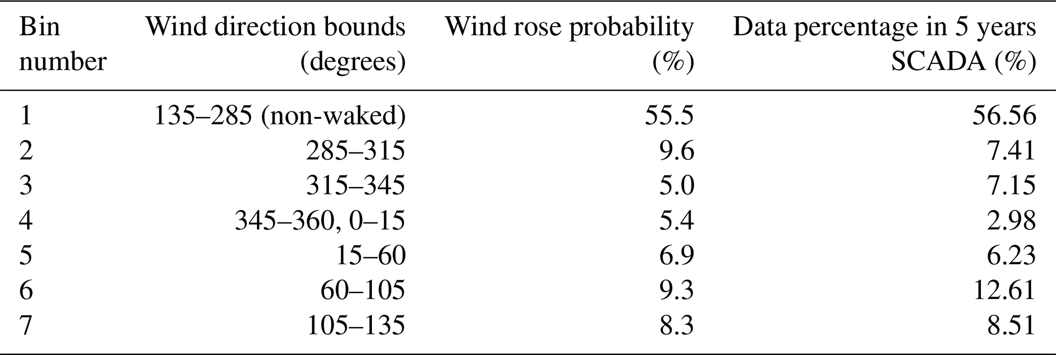
As illustrated in Table 1, the available data percentage after filtration does not fully match the wind direction probabilities. This is partly because in some heavily waked conditions the turbine has been shut down and partly because of the short duration of the data gathering. In the current work, we keep the mentioned observation in mind as a limitation. Thus, we proceed by assessing all DEL data collectively for the purposes of fitting, extrapolation, and bootstrapping. Figure A5 (in the Appendix) shows the separate analysis of the DEL data in each wind direction bin. This analysis ranks each bin based on both the highest observed and the expected DEL values. Such ranking should be considered when performing fatigue assessments per bin to ensure more accurate evaluations. However, in this study, we estimate damage accumulation based on the overall dataset. This limitation is further discussed in Sect. 4.

In the current case, different distributions best describing the turbulence in each wind speed in the freestream are used. However, we do not present the details of those fits to be concise. We sample from the distributions and use them as input for aeroelastic simulations in the second part of the study (see Sect. 2.3.2).

2.3.2 Aeroelastic simulations

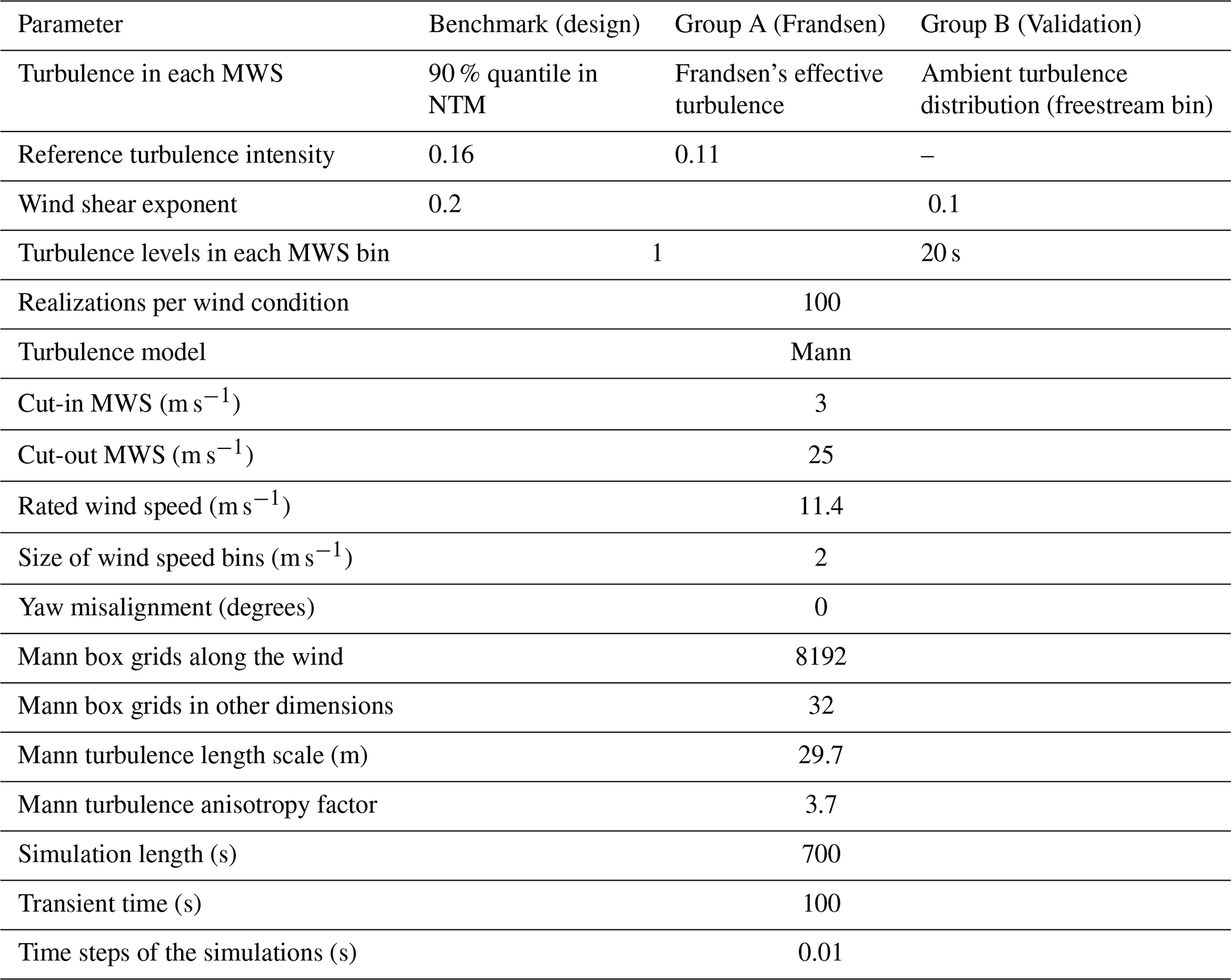
As mentioned before, a generic model of the SWT-2.3 turbine is used in the present study. In this model, the structural and aerodynamic properties were supplied by Siemens Energy, whereas the controller is a tuned version of the DTU 10 MW controller. We conduct all simulations using this model. The benchmark simulations are based on inputs from IEC 61400-1 (International Electrotechnical Commission, 2005) requirements for the design of wind turbine class A. Group “A” is based on the IEC 61400-1 recommendation for site-suitability checks (i.e., the Frandsen model, explained in Sect. 2.4). Group “B” is based on the site-specific inputs in terms of turbulence and wind shear exponents from the freestream (wind bin 1 in Fig. 2). This group of simulations is used solely for the validation of the generic HAWC2 turbine model. The validation results are provided in the Appendix. Groups A and B have 11 mean wind speed bins (from 4 up to 24 m s⁻¹ with 2 m s⁻¹ intervals). Group B only includes the mean wind speeds up to 20 m s⁻¹ as the number of data points and probability of occurrence for the higher mean wind speeds are very low. The first two groups of simulations have one representative turbulence level in each mean wind speed bin. This level equals the 90 % percentile value in group A and the Frandsen waked turbulence level in group B (more details are provided in the next section). We consider 100 seeds for each wind condition to account for the variability of the wind (Mozafari et al., 2023b) and have enough data to fit distributions to the resulting DELs. The third group includes 20 samples from the site-specific turbulence standard deviation distribution in each mean wind speed in the freestream directions (wind bin 1). In this group, having nine mean wind speeds in the related wind directions and 100 turbulence seeds for each turbulence level resulted in a total of 22 000 simulations of 10 min duration for the site-specific aeroelastic simulations (group B). Considering the power law for modeling the wind profile in all simulations, we consider the shear exponent equal to 0.2 in the first two groups and equal to 0.1 in group B as an estimation of the shear exponent in smooth terrain (open water) (Yan et al., 2022). This value is also close to the lidar measurements in the site (Liew et al., 2023). We use the Mann turbulence model (Mann, 1998) to generate the simulation turbulence boxes. The boxes contain 8192 evaluation points alongside the wind direction for higher resolution and 32 points in the other two directions. Table 2 shows the specifications of each group of aeroelastic simulations.

Table 2 Specifications of wind modeling in three groups of HAWC2 simulations, corresponding to three study cases.

It should be noted that group 1 is based on Edition 1 of the IEC standard, which represents the common design framework used for the previous generation of wind turbines – and is therefore particularly relevant for lifetime extension assessments today. Alternatively, when a full lognormal or Weibull distribution is used – corresponding to Editions 3 and 4, respectively – the results of the study differ (see Mozafari et al., 2024, for differences).

The following section outlines the mathematical formulations and procedures used in the present study.

2.4 Mathematical formulations

In the current section, first, we introduce the wind characteristics, and then we briefly present the relations for fatigue load assessment and methods for the reliability and importance ranks. Finally, we explain the procedure for forming the database for statistical extrapolation of DEL measurements via bootstrapping.

2.4.1 Probabilistic modeling of wind

In the current study, we only observe two random parameters of the wind field: the mean wind speed and the wind speeds' standard deviation (i.e., turbulence). Following the IEC standard (International Electrotechnical Commission, 2019), we assume the distribution of the mean wind speed at hub height to be Rayleigh for both cases of design-level assessment and site-suitability check (the Frandsen model). In the latter, the mean wind speed in the waked area is assumed to be the same as the freestream. For site-specific assessments under non-waked conditions, the measured distribution of wind speed is used directly, as it more accurately reflects the actual conditions at the site. In the case of design-based assessment, we use the 90 % quantile of the lognormal distribution as suggested by the normal turbulence model in International Electrotechnical Commission (2005) as the representative turbulence. Equation (1) presents this level.

$$\begin{array}{}\text{(1)}& {\mathit{\sigma }}_{\text{rep. design}}=I_{\mathrm{ref}}(\mathrm{0.75}{v}_{\mathrm{hub}}+\mathrm{5.6})\end{array}$$

In Eq. (1), I_ref is the reference turbulence intensity equal to 0.16 for the standard class 1 wind turbines (the current case study). In addition, V_hub is the hub height wind speed.

In the Frandsen model, the freestream standard deviation is assumed to be the 90 % quantile of a normal distribution, as in Argyle et al. (2018). In the waked conditions, the turbulence is described as a function of the thrust coefficient and the normalized distance of the closest wind turbine. Equations (2) and (3) present the freestream standard deviation formulations and enhanced turbulence due to wakes in the Frandsen model.

$$\begin{array}{}\text{(2)}& {\mathit{\sigma }}_{\text{rep. Frandsen}}={\mathit{\mu }}_{\mathit{\sigma }}+\mathrm{1.28}\times {\mathit{\sigma }}_{\mathit{\sigma }}\end{array}$$

In Eq. (2), σ is a random variable representing the standard deviation of the freestream wind. In addition, μ_σ and σ_σ refer to the mean and standard deviation of the turbulence, respectively. In scenario 1 of the present study, these values are obtained from measurements corresponding to the freestream wind direction bin.

$$\begin{array}{}\text{(3)}& T_{\mathrm{waked}}\left(\mathit{\theta }\right)=\sqrt{{\displaystyle \frac{v_{\mathrm{hub}}^{\mathrm{2}}}{{\left(\mathrm{1.5}+\mathrm{0.8}\left(\frac{d_i\left(\mathit{\theta }\right)}{\sqrt{C_{\mathrm{T}}}}\right)\right)}^{\mathrm{2}}}}+{\mathit{\sigma }}_{\text{rep. Frandsen}}^{\mathrm{2}}}\end{array}$$

In Eq. (3), θ is the (wind) direction in which the waked turbulence is estimated, d_i(θ) is the distance of the closed turbine in that direction normalized by the rotor diameter, and C_T is the characteristic value of the wind turbine thrust coefficient for the corresponding hub height wind velocity (International Electrotechnical Commission, 2019). We use the thrust coefficient data provided in Montavon et al. (2009) for the current study.

The Frandsen model's turbulence is the same in all wind directions (like in IEC design assessments). This independence from wind direction is obtained by effective turbulence. Equation (4) shows the effective turbulence used for site-suitability checks (International Electrotechnical Commission, 2019).

$$\begin{array}{}\text{(4)}& T_{\mathrm{eff}}\left(V_{\mathrm{hub}}\right)={\left(\sum _{\mathit{\theta }=\mathrm{0}}^{\mathrm{2}\mathit{\pi }}{P}_{\mathit{\theta }}\left(V_{\mathrm{hub}}\right)\left(T_{\mathrm{waked}}\right(\mathit{\theta }){)}^m\right)}^{\frac{\mathrm{1}}{m}}\end{array}$$

In Eq. (4), P_θ(V_hub) is the probability of occurrence of the hub height mean wind speed in each direction (θ), and m is the fatigue (Wöhler) exponent (Basquin, 1910).¹

2.4.2 DEL estimation

In the present research, we use the Basquin relation (Basquin, 1910) to model the fatigue resistance of the composite material and Palmgren–Miner's (or Miner's) rule (Palmgren, 1924; Miner, 1945) to model the damage accumulation. These models describe the lifetime and damage as functions of stress, while the outputs of the aeroelastic simulations that we use are flapwise bending moments in the blade root. Since the location of interest (the strain gauge installation location) is close to the root and nearly circular, we use Eq. (5) to obtain the stresses based on the moment time series.

$$\begin{array}{}\text{(5)}& S_i={\displaystyle \frac{M_{x_i}\times c}{I_y}}\end{array}$$

In Eq. (5), $M_{x_i}$ denotes the bending moment corresponding to the stress level S_i. We evaluate the moments (M_x) accounting for flapwise moments in the blade root. The section parameters c and I_y represent the maximum distance from the neutral axis and the second moment of inertia about the axis perpendicular to the moment direction, respectively. Due to confidentiality constraints, the specific values of these parameters are not disclosed.

Using rainflow counting (Endo et al., 1967) of the moments in each 10 min simulation and the models mentioned (Basquin and Palmgren–Miner), we estimate the 10 min fatigue damage via Eq. (6).

$$\begin{array}{}\text{(6)}& D={\left({\displaystyle \frac{c}{I_y}}\right)}^m\sum _{i=\mathrm{1}}^{N_s}{\displaystyle \frac{n_i\times (M_{x_i}{)}^m}{k}}\end{array}$$

In Eq. (6), N_s is the total number of rainflow-counted bins. In addition, m is the fatigue exponent, and k is the Basquin coefficient (see Basquin, 1910). Reformulation of Eq. (6) using the concept of DEL (see Mozafari et al., 2023b, for more information) results in Eq. (7). We use this expression in the current study to simplify the comparisons.

$$\begin{array}{}\text{(7)}& D={\displaystyle \frac{N_{\mathrm{eq}}\left({\mathrm{DEL}}_{\mathrm{lifetime}}^m\right)}{k}}{\left({\displaystyle \frac{c}{I}}\right)}^m\end{array}$$

In Eq. (7), N_eq is the reference number of cycles. We set N_eq equal to 600 cycles, corresponding to an average of 1 Hz cyclic loading. In addition, DEL_lifetime (the expected value of the fatigue damage equivalent load through lifetime) can be derived from 10 min DEL estimations via Eq. (8).

$$\begin{array}{}\text{(8)}& \begin{array}{rl}E\left({\mathrm{DEL}}_{\mathrm{lifetime}}^m\right)& =\sum _{\mathrm{\Theta }={\mathrm{\Theta }}_L}^{{\mathrm{\Theta }}_U}\sum _{V_{\mathrm{\Theta }}=V_L}^{V_U}\sum _{T_{(\mathrm{\Theta },V)}=T_L}^{T_U}\\ & \times \left[\right({\mathrm{DEL}}_{\mathrm{10}\text{min},\mathrm{\Theta }}{)}^m\left]\mathrm{P}\right(T,V\left|\mathrm{\Theta }\right)\mathrm{P}\left(\mathrm{\Theta }\right)\end{array}\end{array}$$

In Eq. (8), the parameters Θ_L and Θ_U represent the lower and upper bounds of wind direction bins, respectively. Similarly, V_L and V_U denote the lower and upper bounds of the mean wind speed, while T_L and T_U correspond to the lower and upper bounds of turbulence intensity within each wind direction bin. Furthermore, $P(T,V|\mathrm{\Theta })$ denotes the joint probability of turbulence intensity and mean wind speed within a given wind direction bin Θ. Since we consider the marginal probability of turbulence conditioned on mean wind speed, P(T|V), and the probability of mean wind speed conditioned on wind direction, P(V|Θ), the joint probability can be expressed as the product of these conditional probabilities.

In assessments where a constant turbulence level is assumed for each mean wind speed (i.e., Frandsen effective turbulence and IEC representative turbulence characterizations), the probability of the single turbulence value is set to 1. In contrast, for group 3 simulations, the probability distribution of turbulence within each wind speed bin is explicitly accounted for, while the probability of the wind direction bin is set to 1, since only wind direction bin 1 is considered for model validation. In measurement-based assessments, the lifetime DEL is estimated using the unweighted average of DEL_10 min, under the assumption that the dataset is sufficiently large for the underlying wind condition probabilities to be implicitly captured. In other words, the distribution of 10 min DEL values inherently reflects the probability distribution of the wind conditions.

Equation (9) defines the relationship between the available n values of DEL_10 min and the corresponding lifetime DEL, DEL_lifetime.

$$\begin{array}{}\text{(9)}& {\mathrm{DEL}}_{\mathrm{lifetime}}^m=\sum _{i=\mathrm{1}}^n{\displaystyle \frac{({\mathrm{DEL}}_{\mathrm{10}{\text{min}}_i}{)}^m}{n}}\end{array}$$

In Eq. (9), in the case of DEL in 1 year, n would be the number of 10 min occurrences within the timeline of 1 year. If enough DEL_10 min data are not available, one has two options: statistical extrapolation (as in the current study) or assuming that the same observations repeat during the longer time spans (for a reference to the importance of statistical extrapolation in the estimation of DEL_lifetime, see Mozafari et al., 2023a, and Mozafari et al., 2023b).

2.4.3 Forming the DEL database based on measurements and statistical extrapolation

For the site-specific (measurement-based) assessment of reliability, we need to obtain the distribution of log (DEL_lifetime) in each year to put in Eq. (14) to be able to estimate the annual reliability level up to year 30 using Eq. (16). We prepare the data for such assessments for up to 30 years. The below steps show the procedure:

1. fitting a distribution to the 10 min DEL measurements

2. extrapolating the fitted distribution from step 1 to estimate higher quantiles representative of a 30-year return period (Eqs. 10 to 12)

3. taking 500 (more than sufficient according to Mozafari et al., 2023b) random samples of size $\mathrm{365}\times \mathrm{24}\times \mathrm{6}\times N$ from the database with replacement, where N accounts for the number of years, and repeating from year 1 to 30

4. calculating the mean of (DEL_10 min)^m in each of the 500 samples and estimating the corresponding DEL_lifetime based on Eq. (9)

5. calculating the logarithm of all generated data and fitting the probability distribution to the 500 realizations of log (DEL_lifetime) in each year.

To form the database (step 2 above), first, we find the probability of exceedance corresponding to the 30-year return period using Eqs. (10) and (11). The extrapolation is used to complete the tail of the DEL_10 min distribution to account for the highest values that might change the weighted mean value (DEL_lifetime) if included. As we are aiming at adding these low-probability high-magnitude occurrences, extreme value theory can be a suitable model to use. These values can have a large effect due to the high fatigue exponent of the composite (Mozafari et al., 2023b).

$$\begin{array}{}\text{(10)}& {\displaystyle }\mathrm{CDF}\left(L_{\mathrm{R}}\right)=\exp \left({\displaystyle \frac{-\mathrm{1}}{T_{L_{\mathrm{R}}}}}\right)\text{(11)}& {\displaystyle }{\mathrm{Pr}}_{\mathrm{exc}.}\left(L_{\mathrm{R}}\right)=(\mathrm{1}-\mathrm{CDF}(L_{\mathrm{R}}\left)\right)\end{array}$$

In Eqs. (10) and (11), CDF accounts for the cumulative distribution function, and L_R accounts for the return load level. Additionally, $T_{L_{\mathrm{R}}}$ in Eq. (10) accounts for the ultimate time of interest for which the corresponding load is estimated. Equation (10) is extracted from the formula of probability of exceeding a threshold level (here the load with a frequency of occurrence of every 30 years), assuming a Poisson process for describing the peak-over-threshold problem (for further information, see de Oliveira, 1984). In the current case, the frequency of exceedance is $\mathrm{1}/T_{L_{\mathrm{R}}}$. It has to be noted that Eq. (10) is correct when $T_{L_{\mathrm{R}}}$ is relatively large (here, equal to the number of 10 min occurrences in 30 years). We set the time in terms of the number of 10 min occurrences because we consider the DEL to be the load, and in this case, each DEL is an occurrence of a 10 min duration. Pr_exc.(L_R) in Eq. (11) is the probability of exceeding such a load, meaning the probability that a load higher than that level occurs. In the case of return loads, this probability is normally very low. We use the CDF corresponding to the return period, obtained from Eq. (10), to find the return load in our case. This load can be derived by finding the inverse CDF of the distribution of our 10 min data (step 1 above). After finding the higher load, we can find the number of occurrences of each DEL level in our database based on Eq. (12). In other words, first, the loads with a certain reference return period are defined, and the frequency of lower loads is derived accordingly.

$$\begin{array}{}\text{(12)}& i={\displaystyle \frac{\mathrm{1}}{\mathrm{Pr}\left(L_{\mathrm{R}}\right)}}\end{array}$$

In Eq. (12), i is the number of occurrences of each 10 min DEL level (${\mathrm{DEL}}_{\mathrm{10}{\text{min}}_i}$*), and Pr(L_R) is the probability of occurrence of the return load based on the distribution of DEL_10 min (distribution in step 1 above). Equation (12) is based on the assumption that the probability density functions of DEL_10 min remain the same when more observations are added to the tail through time. The more data involved in fitting the distribution of DEL_10 min, the more accurate this assumption is.

2.4.4 Fatigue reliability estimation

Fatigue reliability assessment is performed to obtain an estimation of the probability of the survival of a structure. Equation (13) presents a mathematical representation of this concept.

$$\begin{array}{}\text{(13)}& R\left(t\right)=\mathrm{1}-P_{\mathrm{f}}\left(t\right)\end{array}$$

In Eq. (13), P_f(t) is the probability of failure at time t. Commonly, this problem is referred to with a function named limit state function (g(x,t)), and the safe region is where this function is positive. Thus, the probability of failure would be the probability of lying in a region in the space of random variables where the limit state function is negative or equal to zero. We fully follow the methods and procedures used in our previous work (Mozafari et al., 2024) for reliability estimation. Here, we present a brief introduction and the general approach. We recommend that readers check Mozafari et al. (2024) for further details. Following Miner's rule, failure is predicted to happen when damage is higher than a threshold level (commonly 1). This rule contains uncertainty due to simplified assumptions like linear damage accumulation without a sequence effect. To account for the uncertainty in Miner's rule, we assume the threshold (Δ) as a random variable with a mean value equal to 1. Thus, the reliability (being the probability of survival) would be the probability of damage being less than Δ. Equation (14) describes the limit state function considering DEL, K, and Δ as random inputs for the case of flapwise bending moments in the blade root with a circular cross section and structural properties of I_y and c (moment of inertia and radius of the cross section, respectively). The time is omitted from Eq. (14) for simplicity, with the assumption that all variables refer to a certain time (t=lifetime).

$$\begin{array}{}\text{(14)}& \begin{array}{rl}g(X,\mathrm{lifetime})& =\log \left(\mathrm{\Delta }\right)-\log \left(N_{\mathrm{eq}}\right)-m\times \log \left({\displaystyle \frac{c}{I_y}}\right)\\ & +\log \left(K\right)-m\times \log \left({\mathrm{DEL}}_{\mathrm{lifetime}}\right)\end{array}\end{array}$$

The parameters log (N_eq) and $m\times \log \left(\frac{c}{I_y}\right)$ in Eq. (14) are constants. Thus, the above equation consists of three random parameters:

• the linear damage accumulation model (log (Δ))

• material resistance (log (K))

• load (log (DEL_lifetime)).

We perform the probabilistic reliability assessment using a first-order reliability method (FORM) in the current work to find the probability that the function g in Eq. (14) can be positive (fatigue reliability). The same approach also provides the importance rank of the random variables (sensitivity of the reliability to each) and is used here (see Mozafari et al., 2024, for details and formulations). We use the reliability index (shown in Eq. 15) as a commonly used measure of structural reliability.

$$\begin{array}{}\text{(15)}& \mathit{\beta }=-{\mathrm{\Phi }}^{-\mathrm{1}}\left(P_{\mathrm{f}}\right)\end{array}$$

The operator Φ⁻¹, shown in Eq. (15), corresponds to the inverse CDF of the standard normal distribution.

We consider the stress ratio R=10 for fatigue properties (SN curve) of the composite (Mikkelsen, 2020). Although the variability of data is included as the coefficient of variation (CoV) of such a curve, a calibration is added at the end to set the mean value of material strength to a certain level at which the target level of reliability is obtained at year 20.

To apply FORM analysis, first, we fit distributions to the estimations of log (DEL_lifetime) calculated based on 10 min simulations using Eq. (9) for the measurement-based assessment and Eq. (8) for the simulation-based scenarios. To model the uncertainty in the model and material properties in the current study, we gather information regarding the distributions and statistical parameters from the literature. Table 3 shows this information together with the references for the coefficients of variation. The mean of the material resistance is found through calibration. The calibration process entails finding a resistance mean value for which the target reliability is achieved at the end of the design lifetime.

Toft and Sørensen (2011); Toft et al. (2016)Fraisse and Brøndsted (2017)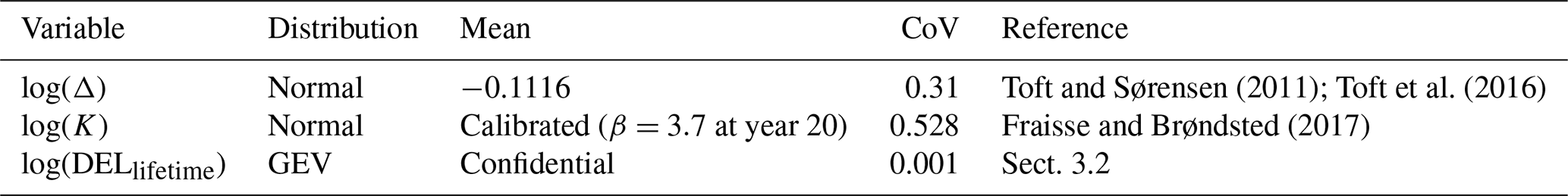

Table 3 Characteristics of the random variables.

Equations (16) and (17) present the formulations for calculating the probability of failure and reliability index at time t (P_f(X,t) and β(X,t), respectively) conditional on survival in the previous point of time (t−Δt) considering a time interval of Δt. The parameter X is a vector of all random variables (the above-mentioned parameters for the current case study). For further information regarding the derivation of Eqs. (16) and (17), see Faber (2012).

$$\begin{array}{}\text{(16)}& {\displaystyle }\mathrm{\Delta }{P}_{\mathrm{f}}(X,t)={\displaystyle \frac{P_{\mathrm{f}}(X,t)-P_{\mathrm{f}}(X,t-\mathrm{\Delta }t)}{(\mathrm{1}-P_{\mathrm{f}}(X,t-\mathrm{\Delta }t\left)\right)}}\text{(17)}& {\displaystyle }\mathrm{\Delta }\mathit{\beta }(X,t)=-{\mathrm{\Phi }}^{-\mathrm{1}}\left(\mathrm{\Delta }{P}_{\mathrm{f}}\right(X,t\left)\right)\end{array}$$

In the current work, we consider Δt to be equal to 1 year, and thus the parameters ΔP_f(X,t) and Δβ(X,t) correspond to the annual probability of failure and annual reliability index and are referred to as such in the continuing discussion. It must be noted that the Frandsen and IEC turbulence models, together with partial safety factors, are intended for semi-deterministic design and not for probabilistic design and reliability analysis. However, since the partial safety factors are calibrated based on achieving a certain reliability level at the end of the design lifetime, the results are comparable. Such comparisons are presented in the next section.

3 Results and discussions

We validate the model of the turbine before performing the study (see the Appendix for validation results). The current section presents the results in three parts: turbulence comparison (Sect. 3.1), fatigue load comparison (Sect. 3.2), and fatigue reliability comparison (Sect. 3.3). The reliability assessment also includes the sensitivity of the reliability level to different random inputs at the target extended life (30 years) in all approaches. Finally, we present the overall discussions on the results in Sect. 3.4.

3.1 Comparison of turbulence levels

Figure 3 presents the comparison between site-specific turbulence based on met-mast anemometer measurements classified in different direction bins, the Frandsen model, and the IEC design class in different wind direction bins. The plot of each direction bin only includes the mean wind speed bins in which there are enough available data to cover the comparison (more than 20 points). The boxes in the whisker plots in Fig. 3 represent the data between the 25th and 75th percentiles, while the dashed black lines indicate the 5th and 95th percentiles. The red plus signs denote data points in the upper and lower tails, as well as potential outliers.

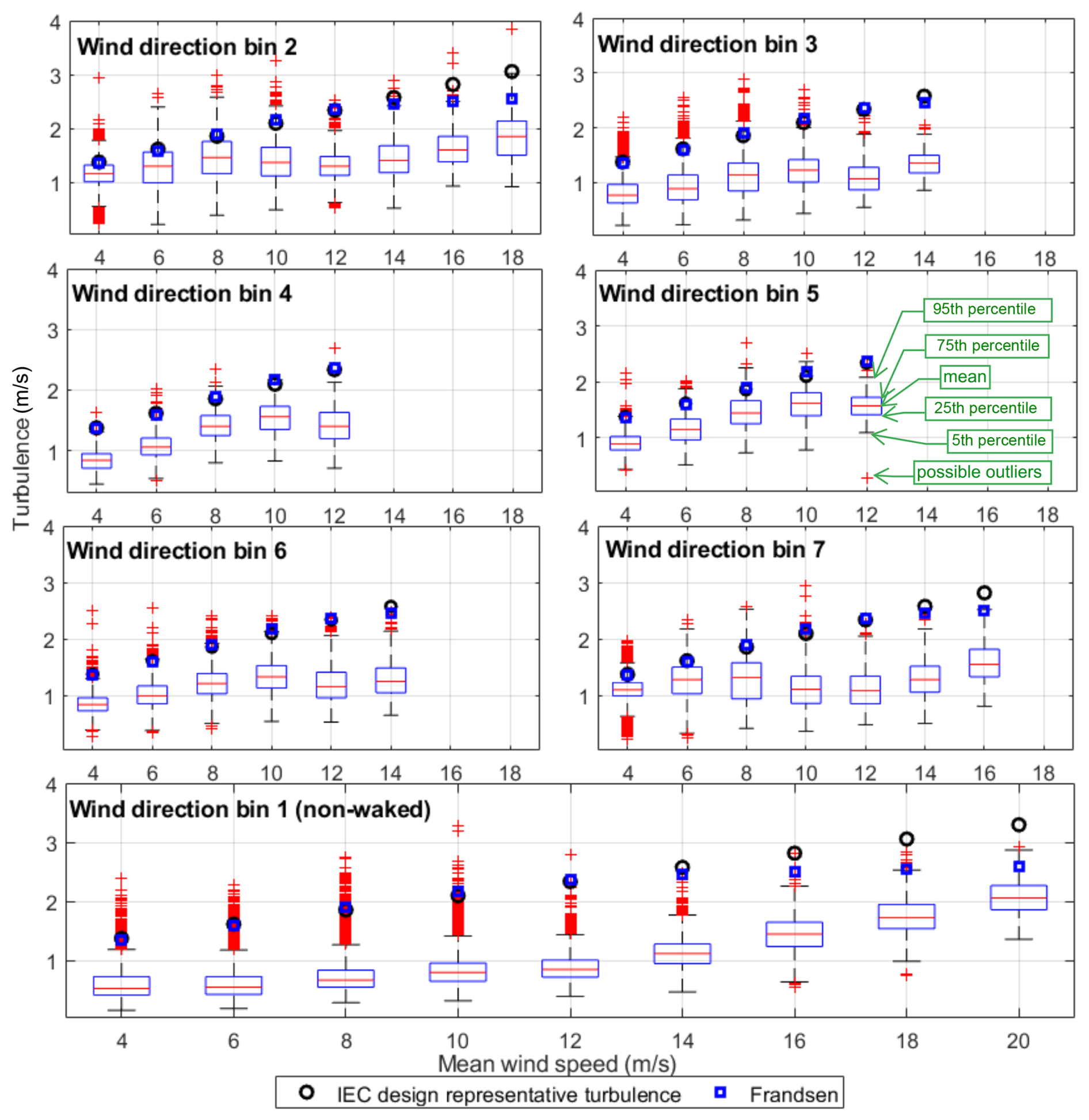
Figure 3 The enhanced turbulence (m s⁻¹) based on Frandsen estimation (blue squares) compared with IEC design representative turbulence (black circles) and the site turbulence measurements (box plots).

The scatter of turbulence versus the corresponding 10 min DEL measurements across different direction bins is provided in the Appendix (see Fig. A4 for an overview of the high-turbulence points relative to the main data clusters). It should be noted that the location of the turbulence measurements differs slightly from the turbine location. Consequently, in some directions, greater deviations may occur between measured turbulence and what the turbine actually experiences due to specific wake effects. Such errors are negligible in freestream directions and higher in other directions. Assuming no outliers in the turbulence measurements and accepting the data as presented, Fig. 3 shows that, in wind bin 1 (freestream conditions), the IEC design turbulence is lower than some of the measurements in low wind speeds but is higher than almost all measurements at higher wind speeds. In addition, Frandsen model estimations are lower than design in high mean wind speeds while being the same as IEC representative values in low mean wind speeds. Emeis (2014) claims the same results for the case of design-level turbulence. This trend remains the same in almost all other wind direction bins. Direction bins 2 and 4 include very high wake effects and high turbulence levels and show less conservative assumptions by the IEC class and the Frandsen model, even in high mean wind speeds. Figure 3 reveals that in some cases, the IEC design turbulence for the class does not lead to much higher levels compared to the Frandsen model. In the following section, we investigate the differences in terms of fatigue loads and fatigue reliability as more accurate parameters to estimate the lifetime extension based on each turbulence estimation approach.

3.2 DEL_lifetime distributions

As shown in Eq. (14), finding the distribution of log (DEL_lifetime) is a necessity for estimating the probability of failure. The current section presents the distribution of DEL_lifetime and log (DEL_lifetime) based on measurement data (DEL_10 min). First, we observe the empirical probability distribution of the 10 min DEL measurements, from which we evaluate DEL_lifetime realizations. Figure 4 shows the empirical probability density of the 10 min damage equivalent flapwise moment from what is measured at the site.

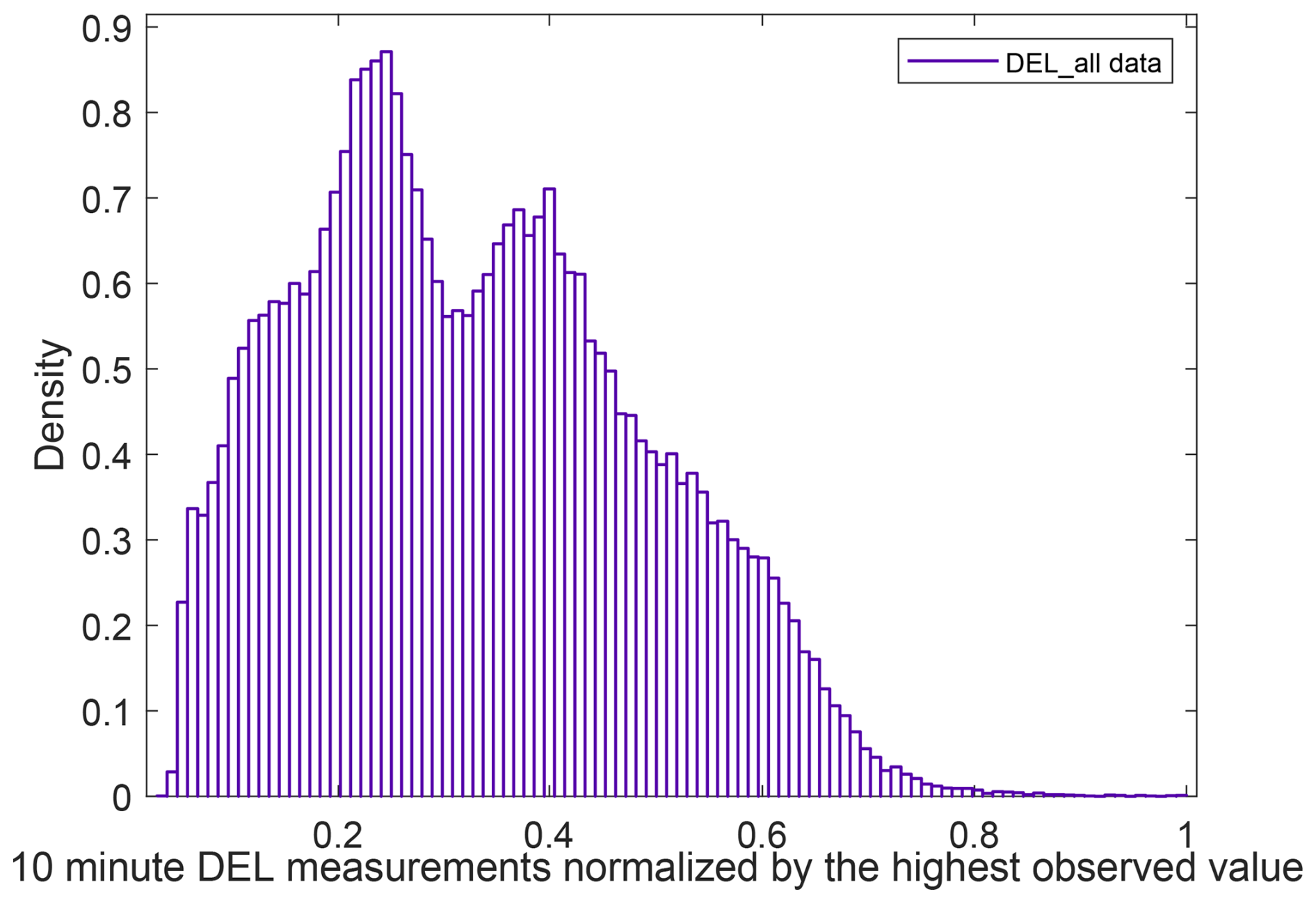
Figure 4 Empirical probability density of the 10 min DEL measurements in all directions combined.

As revealed by Fig. 4, the distribution of the 10 min DEL data is multimodal and cannot be represented fully by unimodal distributions. The multimodality of the DEL can be a result of having both stratified and unstratified winds during the observation time, as the same behavior can be seen in each wind direction bin (see Fig. A5 in the Appendix). We investigate the mixture of two or three gamma distributions, as well as a mixture of two or three Gaussian distributions, as multimodal distributions have shown good candidacy for modeling of fatigue loads (see Mozafari et al., 2023a; Zhang et al., 2022). Among all, the mixture of two gamma distributions appears to be the best fit for describing the statistical behavior of the 10 min damage equivalent flapwise moments in the case study wind turbine's blade root in all direction bins combined. Figure 5 shows this fit on the empirical CDF of data combined.

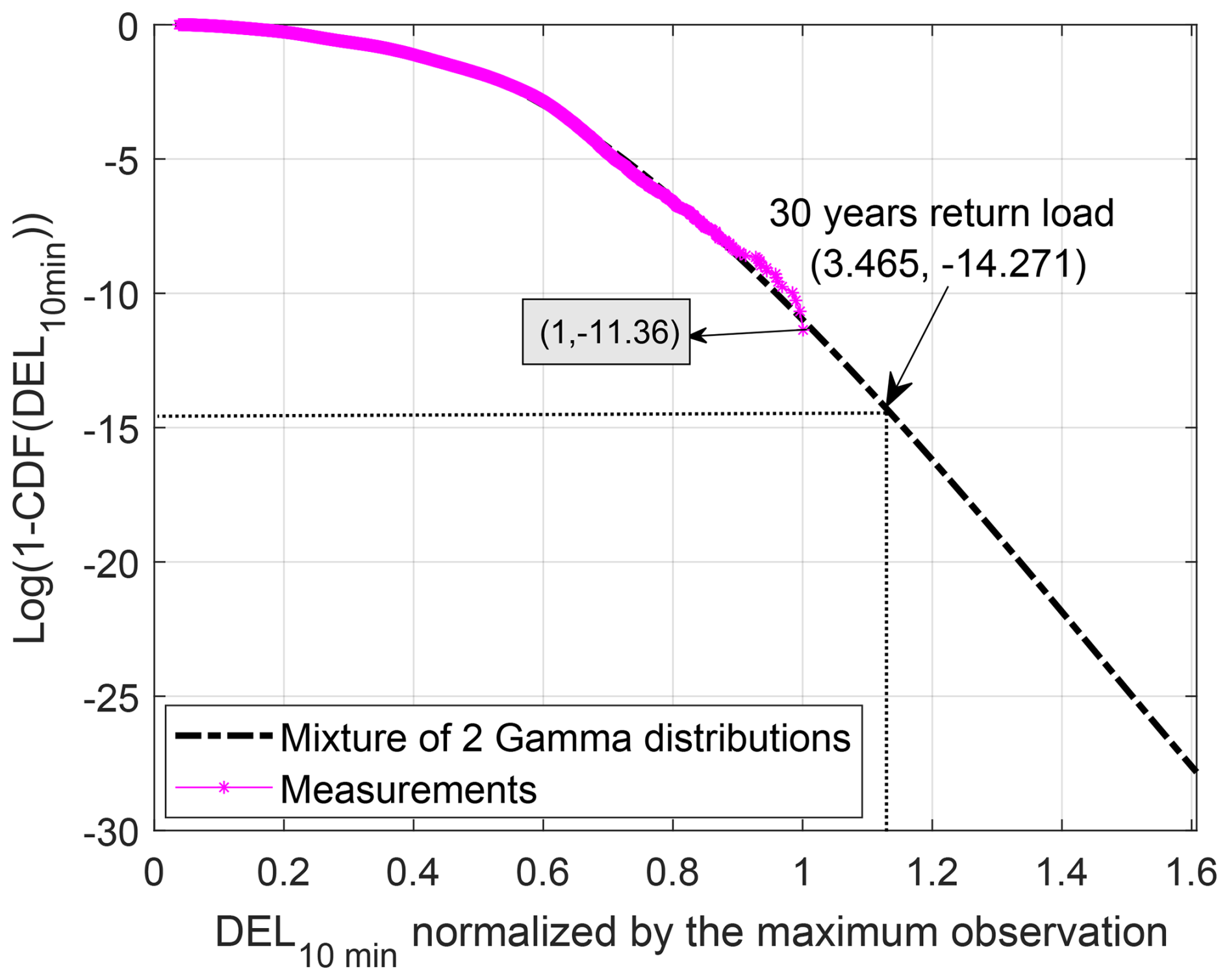
Figure 5 Probability of the exceedance of the DEL based on the empirical cumulative distribution function (purple stars) and based on the best distribution fit to the data (dashed black line).

As presented in Fig. 5, the gamma mixture model fits the data well, with fair accuracy in the higher tail. We use the probability of exceedance from this model and follow the steps presented in Sect. 2.4.3 to find the return load corresponding to 30 years. We use Eqs. (10) and (11) to extrapolate the distribution to the load with a 30-year return period. The slow growth of the tail from year 5 (corresponding to the probability of the largest data point observed) to year 30 shows that the distribution is fairly converged, and a 5-year return period is enough for the main assumption in Sect. 2.4.3 (extreme value theory) to hold. Continuing the procedure with bootstrapping, as outlined in Sect. 2.4.3, the realization of DEL_lifetime in different years is shown in Fig. 6.

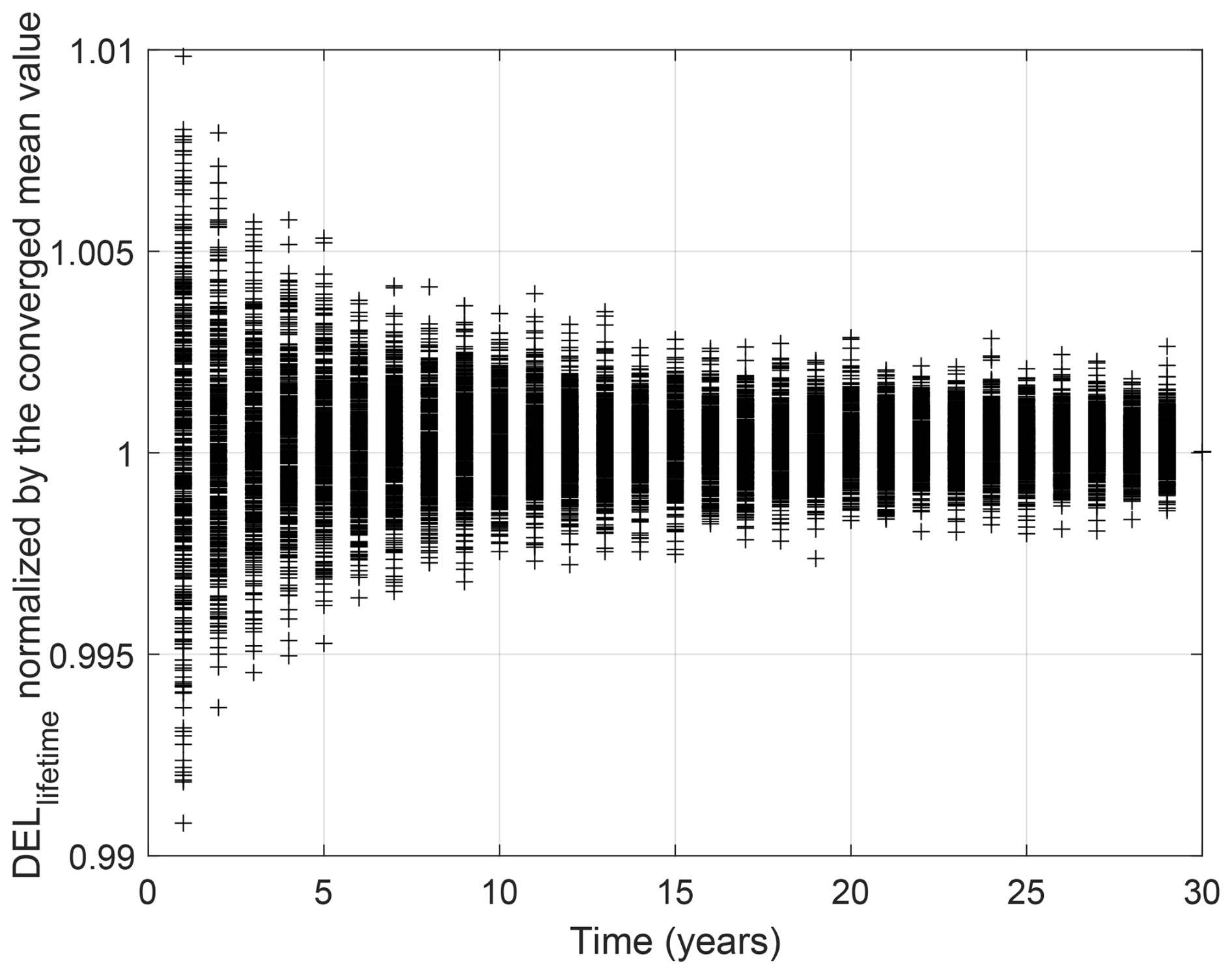
Figure 6 The realizations of DEL_lifetime generated via bootstrapping of available 10 min DEL estimates derived from measurement data.

As shown in Fig. 6, the mean value of the DEL_lifetime realizations converges (with very small changes) as their standard deviation decreases. This complies with our expectation according to the law of large numbers: the mean converges to the “true” expected value of DEL_lifetime as we gather more observations (samples) throughout the years. The change in the standard deviation with a slight change in the mean value allows for the assumption of nonlinear damage accumulation through time (variable DEL through time). We use the converged distribution of DEL_lifetime at year 30 for the estimation of the annual reliability index.

Figure 7 presents the probability density function (PDF) of DEL_lifetime in two different turbulence scenarios of the IEC 61400-1 representative design value and the Frandsen estimation using bootstrapped data among simulations. The uncertainty in log (DEL_lifetime) at the site is modeled by a frequentist approach (maximum likelihood) based on observations and includes all sources of uncertainty. However, in the case of the other two approaches, the uncertainty in this parameter is assessed based on bootstrapping, and thus it only includes epistemic uncertainty. The data in Fig. 7 are normalized by the converged mean of DEL_lifetime obtained above using gathered data.

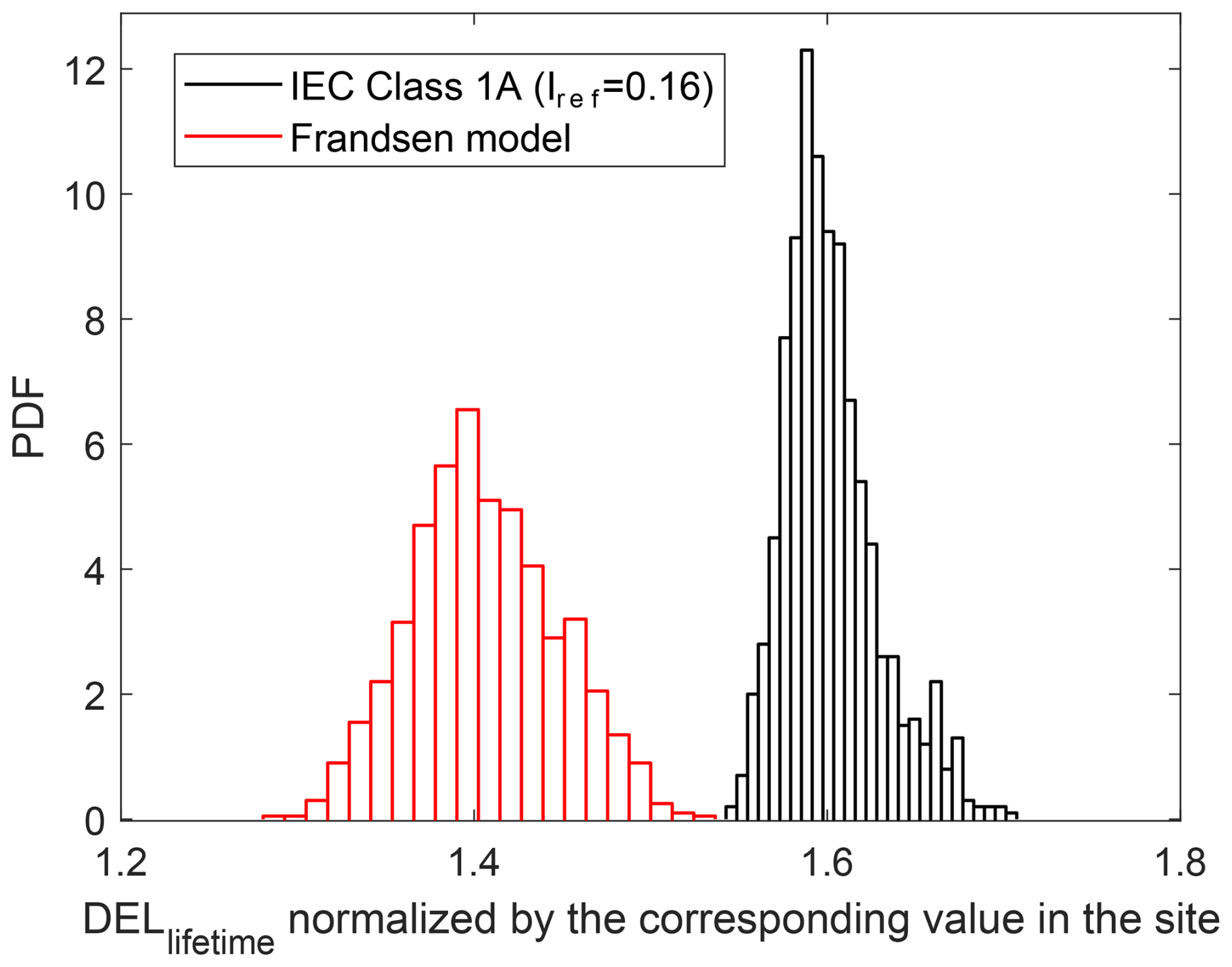
Figure 7 Probability density function (PDF) of DEL_lifetime in two different scenarios of the IEC standard for design and site-suitability checks (based on the Frandsen model) normalized by the mean DEL_lifetime estimation based on the site's measurements.

As shown in Fig. 7, the estimations of DEL_lifetime based on representative design turbulence and the Frandsen method are conservative compared to the site-specific assessment derived from measured turbulence. This is evident from the mean values of the corresponding distributions, which are normalized by the site-specific DEL_lifetime. The Frandsen model, in this case, leads to respectively less conservative fatigue loads than the design-based approach, as expected. In addition, the DEL realizations based on the Frandsen model are more spread out, showing a higher variability. In the following section, we use the DEL_lifetime distribution to assess the fatigue reliability at the end of the design service life and the possible extended life in the above-mentioned scenarios.

As shown in Fig. A2, the resulting 10 min DEL values from simulations in the freestream cover a lower bound of the load measurements at the site. As a consequence, there is bias in lifetime DEL when using the generic aeroelastic model. However, we use the data for estimating the reliability in the next section to illustrate the combined effect of using the Frandsen model and the generic model.

3.3 Reliability and importance ranks

As the turbine model in HAWC2 simulations is generic and the material properties are not defined accurately, we assess the lifetime extension after calibrating the material's mean strength. The calibration is made such that we achieve the target annual reliability index level for a moderate consequence of failure of a structural component (equal to 3.3) (ISO, 2015) at the end of the design life (25 years). Figure 8 presents the annual reliability index for 35 years in all case scenarios based on the calibrated material properties (mean value of strength (K) is multiplied by a factor).

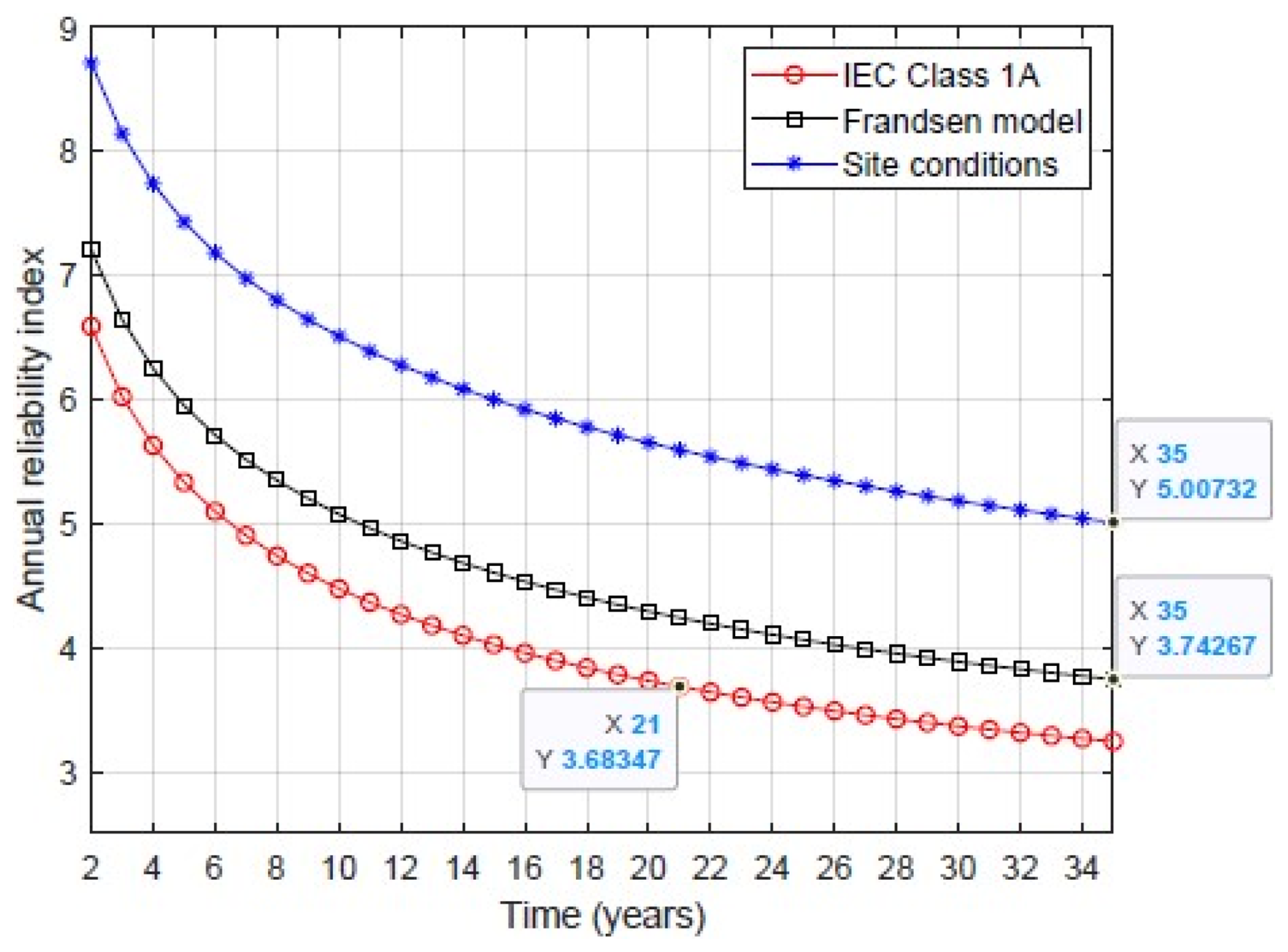
Figure 8 Annual reliability of the case study wind turbine in scenario 1 using the Frandsen model (black square) and in scenario 2 with site load measurements (blue star) versus the IEC design class (red circle).

The difference in the annual reliability levels in different scenarios in Fig. 8 can involve different sources, including the difference in the turbulence (observed in Sect. 3.1), strain gauge calibration, possible missed controlling strategies for the neighboring turbines, and generic model errors. Thus, while the numerical results may not be quantitatively exact, they illustrate an important qualitative principle: with reliable site measurements, the probability of fatigue failure can be continuously updated as operating experience accumulates. The reliability of 3.7 at year 35 for the Frandsen model means that there is a possibility of a lifetime extension of up to 10 years for the turbine under study when using this model. Using the site data, this level is reached in more years, showing the conservative results from the Frandsen model. The steep decline in the design-based annual reliability curve in Fig. 8 represents the high mean value of the design DEL compared to the Frandsen model and site. The big difference between the reliability in the two scenarios is due to the high fatigue exponent of the composite, increasing the effect of the mean of fatigue loads on the reliability. Table 4 shows the importance rank of the random variables in the limit state function (see Eq. 14) based on FORM analysis.

Table 4 The sensitivity of the reliability to different random variables ( %) based on scenario 1 and 3 approaches versus design at year 30.

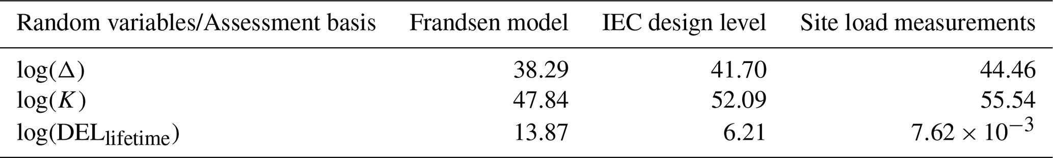
As revealed in Table 4, the relative importance of the load is low in all three scenarios. The relative importance of the fatigue load is higher in the case of the Frandsen model because of the high coefficient of variation of the DEL in this case. Its sensitivity to loads is almost zero when it comes to the site-specific lifetime DEL. The effects of the uncertainty in the material properties are the highest in all cases because of the very high coefficient of variation. In the site assessment, the reliability is highly sensitive firstly to the material uncertainty and secondly to the damage accumulation rule. In other words, the uncertainty in loads almost disappears relative to the other variables when based on measurements on the actual machine.

3.4 Discussion

The data show the conservative estimations of turbulence based on the Frandsen model in high mean wind speeds. The overall DEL estimations using this method are thus conservative when considering the blade's flapwise bending moments. This is despite the aeroelastic model underestimating loads and their variability in freestream conditions (see Table A1). The reliability assessments show the possibility of a lifetime extension for more than 35 years while maintaining safety margins when using the Frandsen method and a generic model.

The difference between the results of the two approaches (Frandsen model and load measurements) stems not only from differences in turbulence inputs, but also from possible generic model errors and strain gauge calibration errors. In this study, the generic model differs from the original only in controller settings, not in structural parameters. Moreover, according to Robertson et al. (2019), the model parameters most relevant to fatigue loads are yaw angle error and certain structural parameters. Therefore, we do not expect generic model uncertainty to account for the majority of the observed error.

The very low sensitivity of the reliability to the fatigue loads in the case of site-specific assessment (using loads measurements) is due to the relatively low coefficient of variation of this variable compared to material strength and Miner's rule. This shows the robustness of DEL_lifetime as an accumulated/averaged random variable. The results comply well with the results shown in Mozafari et al. (2023b), showing how the accumulation decreases the coefficient of variation of DEL_lifetime. Another possible reason for low variation of this parameter is not considering the uncertainty of the fitting in the current work.

There are some limitations and simplifications in the present study that must be considered and improved in future work. As an example, there is a potential difference in the results of the simulation-based approaches if the model was not generic and the simulations were offshore (considering wave loads). The results of the model validation (presented in the Appendix) show that the small differences in load can lead to underestimation of DEL_lifetime in simulation-based scenarios and thus the remaining service life. This is especially important in the assessment based on the Frandsen model and the generic model and as the sensitivity studies show that the reliability of the Frandsen-based approach is sensitive to the loads.

In addition, the results of the current study are performed on the blade flapwise load channel as a case study. However, all the load channels should be investigated when assessing lifetime extension. Specifically, load channels with deterministic behavior (for example blade edgewise moments) often have lower design margins and are thus the critical components deriving the lifetime extension of the wind turbine. The current study does not focus on the actual lifetime of the turbine and but instead focuses on showing the difference between the Frandsen site-suitability assessment and assessments based on site load measurements when it comes to fatigue reliability. Such comparison is more clear on a turbulence-driven fatigue load like flapwise bending moments.

Furthermore, it has to be considered that the data with a return period of 5 years are only referring to the winter season, and thus the tail shape of the distribution might be different if seasonal variability is also included and the data are collected continuously.

Finally, although the turbulence levels from the site and the Frandsen estimation are directly compared, the fatigue load results based on the two are derived differently. The former is based on post-processing of strain gauge data, and the latter is based on aeroelastic simulations. Thus, the possible bias and errors of the turbine model and aeroelastic simulations can affect the DEL and reliability comparison results.

For future work, we recommend the following studies:

1. performing the same study on the performance of the Frandsen model in deeper locations within the wind farm, as they usually include more intense/complicated wake conditions;

2. comparing the use of ambient wind data (using Frandsen) with location-specific measurements of the turbulence considering all the load channels (lifetime extension assessment as a whole) and performing offshore simulations;

3. considering other sources of uncertainty in the reliability assessment framework, e.g., including uncertainty due to range-counting methods or uncertainty in simulations;

4. investigating the reasons behind the multimodality of the 10 min DEL distribution;

5. performing the same study using independent fittings and extrapolations of DEL in each wind bin for higher certainty and accuracy in the assessment;

6. considering the uncertainty of fitting in defining site-specific lifetime DEL and its variability;

7. investigating the sensitivity of the outcome to model parameters under varying environmental conditions (although Robertson et al., 2019, conducted a sensitivity study on how aeroelastic model parameters affect fatigue loads, results for lifetime extension assessments may differ due to their comparative nature);

8. joining the study with inspection and health-monitoring data coupled with risks and cost analysis to obtain a complete set of tools for decision-making regarding lifetime extension.

4 Conclusions

The objective of this study is to demonstrate the significant benefits of collecting and utilizing load/displacement measurements, which can outweigh the challenges of such assessments by extending the project lifetime of wind turbines. The research mainly compares two different data availability scenarios – one with structural response measurements and one without. In addition, it addresses two common challenges in fatigue reliability assessments. First, it evaluates the performance of the Frandsen model in estimating waked turbulence and corresponding fatigue loads at Lillgrund, a compact wind farm with mixed wake conditions. Second, it presents a methodology for extrapolating fatigue loads, showcasing an example application using strain gauge measurements in Lillgrund.

The results indicate that the Frandsen model provides conservative estimates of fatigue loads at the investigated location, despite the compact layout of Lillgrund. This conservatism persists even though the generic model used tends to underestimate fatigue loads relative to the site-specific conditions in the freestream directions.

Additionally, the relative importance of load estimates in assessments based on the Frandsen model is greater than in those based on site load measurements. Due to the way fatigue reliability decreases very slowly over the later years of project lifetime, the reduction in uncertainty created by load measurements at the site can provide the knowledge basis for many additional years of turbine operation within an acceptable reliability target.

The extrapolation approach presented in the current research facilitates the use of data when strain gauge measurements are unavailable for part or all of the turbine's lifespan. The assessment of the Frandsen model in this case study, representing a wind farm with short spacing, contributes valuable insights into ongoing research on the performance of this model in intense and mixed wake conditions. Moreover, the findings on the robustness of reliability based on the load estimation approach are crucial for incorporating uncertainty into lifetime extension assessments.

Above all, the comparison between scenarios with and without load measurement and accurate environmental data shows the importance of having such information coupled with accurate models updating in real time (digital twins).

Appendix A: Model validation

As mentioned in Sect. 2.3.2, simulations in the freestream direction are used for validation of the model. The input is based on site-specific inputs from the non-waked freestream (wind direction bin 1). First, we compare the mean load levels from site measurements in wind bin 1 to the results of the group 3 simulation. Then, we compare the 10 min DEL evaluations and investigate the differences in DEL_lifetime formed via bootstrapping.

Figures A1 and A2 show the comparison of the mean load levels and 10 min DELs in the measurements versus simulations, respectively.

The data shown in Figs. A1 and A2 reveal the high variation in the measured mean load and damage equivalent flapwise moment around rated mean wind speed. The high difference in this area can introduce some errors in the estimations based on simulations (groups 1 and 2) based on dominant (high-probability) wind speeds. However, generally, the data show fair coverage of the site load behaviors.

Figure A3 represents the power production versus mean wind speed compared with the nominal power curve after filtration.

Figure A4 shows that the high tail of turbulence observations mostly belongs to the cluster of data, and the possibility of having a high number of outliers is low. The probability of exceedance of the 10 min DEL measurements within each wind direction bin is shown in Fig. A5 using both the empirical CDF and the best distribution fit to each cluster of data.

Figure A5 shows that the highest DEL observations occur in wind bin 5.

In addition, the data in Table A1 reveal that the load fluctuations in the simulations are very small compared to reality. This is partly because of the integration over turbulence distribution (see Mozafari et al., 2024, for details) and partly due to the variability in the environmental condition (see Sect. 3.1). Although the validations show overestimations of the load and DEL in high mean wind speeds, we proceed with the study using the available HAWC2 model because the differences in the overall DELs shown in Table A1 are less.

Different distributions shown in Table A2 are fitted to the mean wind speed data of the wind turbine. As can be seen, the best fit is the Rayleigh distribution. The maximum likelihood method is used for fitting, and the prediction error is measured by the Akaike information criterion (AIC).

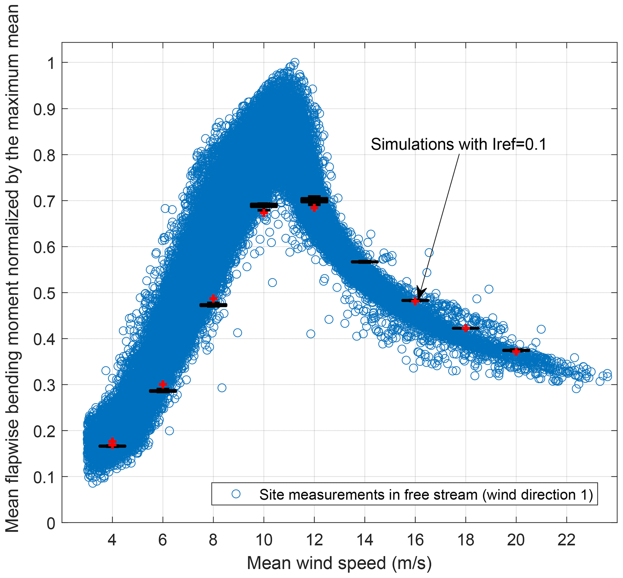
Figure A1 The mean flapwise bending moment in different mean wind speeds (measured by met-mast-mounted anemometers) in non-waked directions from two sources of measurements (blue circles) and simulations (black boxplots).

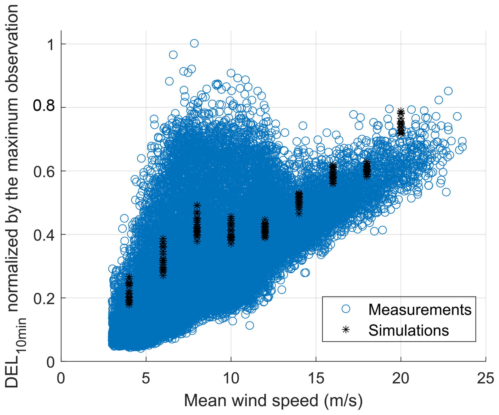
Figure A2 The cluster of 10 min DEL data in the freestream versus the DEL estimations from simulations in each mean wind speed.

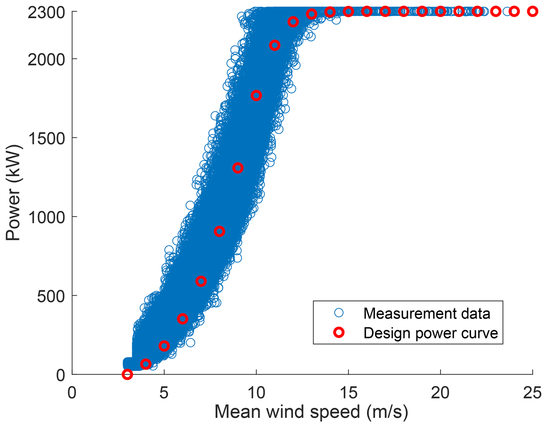
Figure A3 The filtered power production data versus mean wind speed, measured by met-mast-mounted anemometers (blue), compared with the nominal power curve (red).

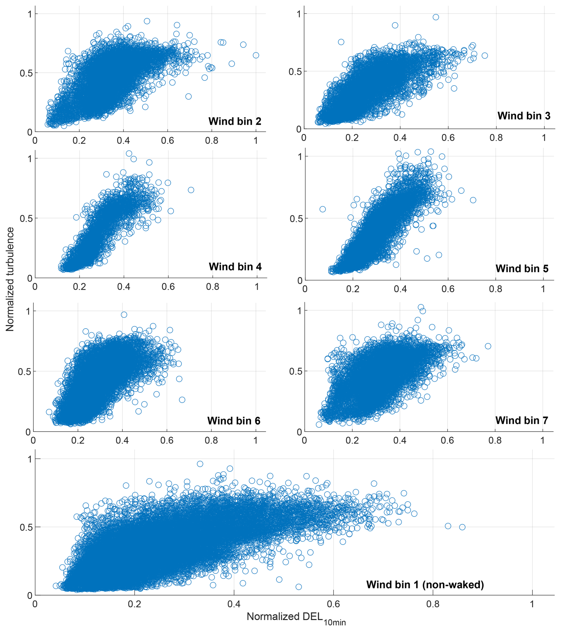
Figure A4 Scatter plot of turbulence data normalized by the highest observations versus corresponding 10 min DEL observations at the same time in different wind direction bins before filtration.

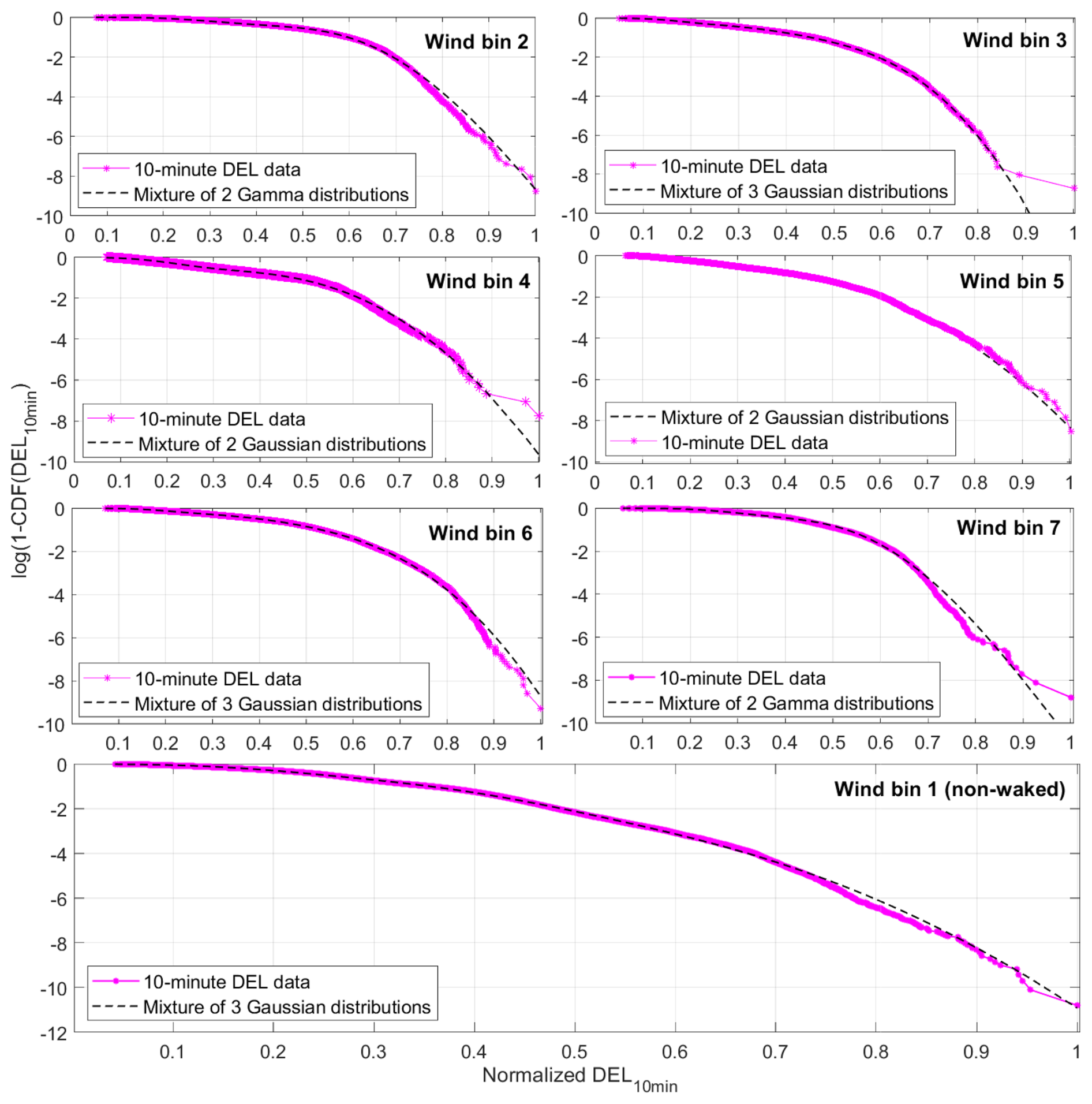
Figure A5 Logarithm of the probability of exceedance of the normalized DEL_10 min in different wind direction bins in the location of the wind turbine (dotted purple line) and the best distribution fits (dashed black line).

Table A1 Statistical parameters of DEL_lifetime according to the non-waked aeroelastic simulations using site-specific turbulence and shear exponent versus the same parameters from measurements.

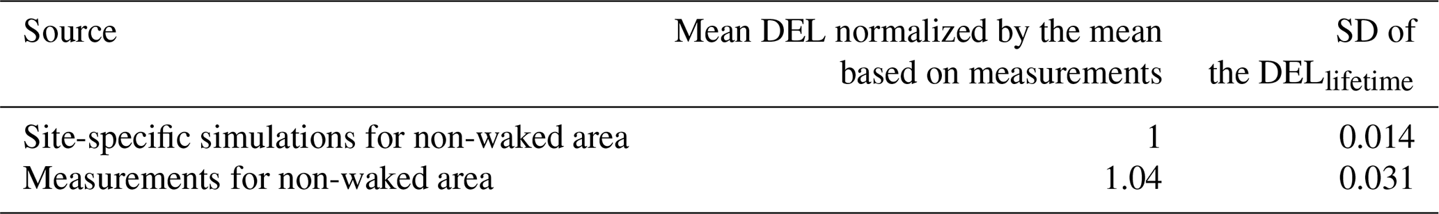
Table A2 Different distributions fitted using the maximum likelihood method to the wind speed measurements, including statistical parameters of the fits (shown as Par1, Par2, and Par3).

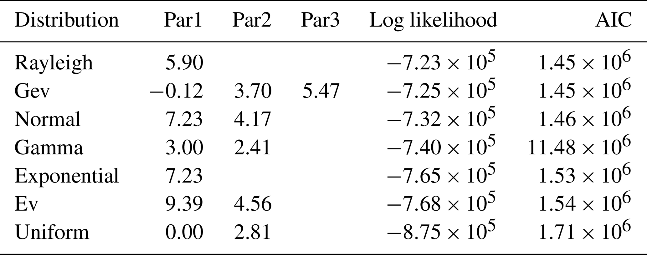
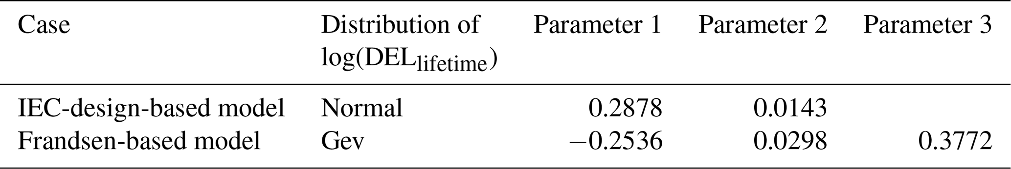
Table A3 The best distribution fits to log (DEL_lifetime) in case scenarios of Frandsen turbulence and the IEC standard's representative turbulence for the freestream direction.