the Creative Commons Attribution 4.0 License.
the Creative Commons Attribution 4.0 License.
 | 24 Sep 2018
Interannual variability of wind climates and wind turbine annual energy production
Tristan J. Shepherd
Rebecca J. Barthelmie
The interannual variability (IAV) of expected annual energy production (AEP) from proposed wind farms plays a key role in dictating project financing. IAV in preconstruction projected AEP and the difference in 50th and 90th percentile (P50 and P90) AEP derive in part from variability in wind climates. However, the magnitude of IAV in wind speeds at or close to wind turbine hub heights is poorly defined and may be overestimated by assuming annual mean wind speeds are Gaussian distributed with a standard deviation (σ) of 6 %, as is widely applied within the wind energy industry. There is a need for improved understanding of the long-term wind resource and the IAV therein in order to generate more robust predictions of the financial value of a wind energy project. Long-term simulations of wind speeds near typical wind turbine hub heights over the eastern USA indicate median gross capacity factors (computed using 10 min wind speeds close to wind turbine hub heights and the power curve of the most common wind turbine deployed in the region) that are in good agreement with values derived from operational wind farms. The IAV of annual mean wind speeds at or near typical wind turbine hub heights in these simulations and AEP computed using the power curve of the most commonly deployed wind turbine is lower than is implied by assuming σ=6 %. Indeed, rather than 9 out of 10 years exhibiting AEP within 0.9 and 1.1 times the long-term mean AEP as implied by assuming a Gaussian distribution with σ of 6 %, the results presented herein indicate that in over 90 % of the area in the eastern USA that currently has operating wind turbines, simulated AEP lies within 0.94 and 1.06 of the long-term average. Further, the IAV of estimated AEP is not substantially larger than IAV in mean wind speeds. These results indicate it may be appropriate to reduce the IAV applied to preconstruction AEP estimates to account for variability in wind climates, which would decrease the cost of capital for wind farm developments.
- Article
(5116 KB) - Full-text XML
- BibTeX
- EndNote


Wind speeds and thus electrical power production from wind turbines (WTs) vary across multiple temporal and spatial scales. Short-term forecasts (hours to days) of wind speeds at or near WT hub heights (and ideally across the swept area of the WT rotor) are key to grid management and electricity pricing (Barthelmie et al., 2008; Orwig et al., 2015) and are exhibiting progressively greater accuracy from direct numerical simulation and statistical post-processing (Pinson et al., 2007; Sperati et al., 2015; Dowell and Pinson, 2016; Wilczak et al., 2015). Monthly to seasonal forecasts are also increasingly available to inform planning for WT and grid maintenance (Yu et al., 2015; Torralba et al., 2017). Variability on intra-annual to decadal timescales (Pryor and Barthelmie, 2011; Pryor et al., 2006) arises primarily due to the action of internal climate modes such as the El Niño–Southern Oscillation (ENSO) (Schoof and Pryor, 2014; Pryor and Ledolter, 2010; Kirchner-Bossi et al., 2015; Bett et al., 2017; Watts et al., 2017) and climate nonstationarity (e.g., climate change due to the rising concentration of heat-trapping gases) (Pryor and Barthelmie, 2010; Pryor et al., 2012a, b; Tobin et al., 2016) and is also key to dictating the electricity produced by WT arrays over their lifetime.
Wind farm developments (i.e., arrays comprising multiple WTs) are highly capital intensive with the fuel being free (Lantz et al., 2012). According to some estimates, capital costs (e.g., purchase of wind turbines, installation of foundations and grid connections) comprise up to 80 % of the total cost of a typical onshore project over its entire lifetime (Blanco, 2009). The ratio of capital expenditure to operational expenditures for wind farms in Germany is approximately 0.69 for onshore and 0.54 for offshore wind farms (Steffen, 2018). While the majority (61 %) of global “conventional” power plants are commissioned by state-owned enterprises, private companies commissioned 53 % of non-hydro-renewable power plants in 2015 (Steffen, 2018). Further, in Germany, wind farms are overwhelmingly funded through project finance (88 % for onshore, 50 % for onshore) rather than corporate finance, again in contrast to traditional power stations (Steffen, 2018). Thus, financing risk is particularly important to wind energy (and other non-hydro-renewables) and to the levelized cost of energy (LCOE). For example, for a project lifespan of 20 years, increasing the cost of capital from 3 % year−1 to 15 % year−1 multiplies the required annual payments by a factor of 2.4 (Krupa and Harvey, 2017).
The cost of capital investments and/or rates of return is determined by the “risk” associated with each wind energy project and hence the annual electricity production and variability therein and the resulting anticipated revenue (Feldman and Bolinger, 2016). The variability of revenue due to meteorological and resource variability is described as a specific risk (Gatzert and Kosub, 2016) and requires a minimum debt service coverage ratio if the financing involves debt. Two metrics are often used to quantify the viability (and risk) of wind projects in terms of the annual energy production (AEP) (i.e., the amount of electricity generated from deployed wind turbines) over the lifetime of existing and planned wind farms.
-
P50: AEP projected to be equalled or exceeded on 50 % of years during wind farm operation (P50(AEP)).
-
P90: AEP that is associated with a 10 % risk of not being reached (P90(AEP)).
Accurate quantification of the wind resource and the P50(AEP) and P90(AEP) presents a significant challenge to current models (Zhang et al., 2015), and even small uncertainties in modeled wind speeds cause major uncertainties in P50(AEP) and P90(AEP) and significantly impact the cost of investment capital in new wind projects (Tindal, 2011; Clifton et al., 2016). Capital investments by the wind energy industry within the United States of America during 2016 are estimated at USD 14.5 billion (Dykes et al., 2017), while estimates of investment in European offshore wind energy are projected to be between USD 90 and 124 billion over the period 2013–2020 (Gatzert and Kosub, 2016). Even small refinements of perceived and actual project risk deriving from the interannual variability of wind speeds may provide tremendous cost efficiencies (i.e., more accurate assessment of financing costs) and contribute to continuing the recent tendency towards reduced LCOE. It has been suggested that the LCOE from wind turbines could be reduced by half to USD 23 per megawatt hour in part due to reductions in financing costs by lowering this long-term production risk (Dykes et al., 2017).
Interannual variability (IAV) is used to describe the year-to-year variability in a given property. According to some estimates, IAV contributes “anywhere between 10 % and 25 %” of the overall uncertainty in project energy yield over a 10-year period (Pullinger et al., 2017). In the wind energy literature IAV is often represented by assuming a Gaussian distribution for annual mean wind speeds and specifying the dispersion of values around that mean in terms of the standard deviation (σ) of annual mean wind speeds to the long-term mean value. IAV is thus often quoted as a percentage of the mean. The IAV for annual mean wind speeds (as described using σ) of 6 % is often quoted within the wind energy industry as a representative estimate (Brower, 2012). Indeed, the website (https://www.wind-energy-the-facts.org/the-annual-variability-of-wind-speed.html, last access: 4 June 2018) states that “the annual variability of long-term mean wind speeds at sites across Europe tends to be similar, and can reasonably be characterized as having a normal distribution with a standard deviation of 6 per cent.” This implies that approximately two-thirds of years will have an annual mean wind speed within ±6 % of the long-term mean. However, much of the research that underpins this assumption is derived from examination of wind speeds at 10 m a.g.l. and employs either data from a limited number of in situ observing stations or relatively coarse-resolution reanalysis output (see the overview of previous research in Table 1). Further, use of the mean and standard deviation to describe the central tendency and dispersion of a sample implicitly makes an assumption that the sample(s) of annual mean wind speeds are Gaussian distributed. In the event that the sample of annual mean wind speeds is not Gaussian distributed, σ is neither a robust nor a resilient measure of dispersion.
Table 1Overview of past research on the IAV of wind climates and a summary of results presented herein. Results from the current study are shown for grid cells that contain areas with currently operating wind farms denoted by the underlining and for all other grid cells; these represent results for 90 % of the grid cells in each class.
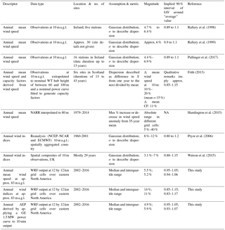
NA: not available
In one of the first published studies on this topic, the IAV of mean wind speeds as described using the σ of annual values around the mean across five surface (i.e., within 10 m of the ground) stations in Ireland ranged from 4.7 % to 6.4 % (Raftery et al., 1998). In a more recent analysis of surface observations from 16 stations, also in Ireland, collected over data periods of up to 13 years, σ was reported to lie between 4.4 % and 6.9 % of the mean (Pullinger et al., 2017). Conversely, an analysis of monthly wind speeds at approximately 80 m over the period 1979–2014 from the North American Regional Reanalysis (NARR) data set found “variations in the wind speed of up to 30 %” at some existing wind turbine locations in the United States (Hamlington et al., 2015).
Wind indices (WIs) have also been used in an attempt to better reflect the IAV of the energy available to be harnessed by wind turbines (Table 1) and are calculated as
where j=1…n, n is the number of years, i…k=normalization period and the mean denotes the spatial average.
The standard deviation of WI integrated over the Scandinavian countries at 10 m of height from both NCEP–NCAR and ECMWF reanalyses during 1960–2001 ranged from 8 %–12 % (Pryor et al., 2006). The σ of WI for the UK computed using observations collected at 10 m varied from 3.1 %–7.0 % depending on the source, number of stations, data period and whether the data were detrended (Watson et al., 2015). Annual WIs generated using Eq. (1) are very sensitive to the frequency of occurrence (and magnitude) of high wind speeds. The actual electrical power derived from wind turbines varies according to the power curves that relate power produced to the wind speed at WT hub height. This power is zero below cut-in wind speeds, increases rapidly as wind speeds increase and is a constant once the wind speed exceeds that necessary to generate the “rated power” (RC) (Fig. 1) until they exceed a cut-out wind speed (of 25 m s−1 for the wind turbine used herein). This nonlinearity in turbine power curves means long-term electricity production is typically dominated by the upper percentiles of the wind speed probability density function, but is relatively insensitive to the occurrence of extremely high wind speeds (i.e., above WT cut-out) assuming that they occur only a small fraction of the time (Pryor and Barthelmie, 2010). In short, the IAV in AEP may not be directly proportional to either the IAV of annual mean wind speeds or WI. Very few studies have quantified the actual IAV in wind farm power output. Power output data from a single individual wind farm in the US over the period 2000–2010 ranged between 0.82 and 1.13 of the long-term mean (Wan, 2012). This range in net AEP naturally includes the impact of other factors such as curtailment and maintenance and does not seek to decompose the variability into the root causes.
Here we investigate IAV in mean wind speeds and WI near typical WT hub heights using purpose-performed numerical simulations with the Weather Research and Forecasting (WRF) model (v3.8.1). We further estimate IAV in likely AEP due to IAV in wind climates by applying the power curve (Fig. 1) from a common wind turbine deployed within the study area to 10 min wind speed output from these simulations. The results are validated and contextualized using net capacity factors (CFs) generated based on power production data from operating wind farms within the simulation domain.

Figure 1Power curve (i.e., expected electrical power production as a function of the hub height inflow wind speed) for the GE 1.5 SLE wind turbine. The three colored bars shown in magenta, grey and green on this figure show the 95 % confidence intervals on the bootstrapped mean annual mean wind speed in the three example grid cells in Texas (TX), Iowa (IA) and New York (NY) state, respectively (see Fig. 2a for the locations of these grid cells).
2.1 Simulations
Herein we present model-based analyses of the IAV in mean wind speeds, WI and estimated AEP using simulations performed with WRF applied at 12 km resolution over the domain shown in Fig. 2a. The domain is extended to the west of the region with the highest numbers of deployed WTs (i.e., the Central Plains) to avoid collocation of the lateral boundaries with a region of strong surface forcing (i.e., the Rocky Mountains). Default settings as specified in the WRF user guide for v3.8 (available at: http://www2.mmm.ucar.edu/wrf/users/docs/user_guide_V3.8/ARWUsersGuideV3.8.pdf, last access: 4 June 2018) are used for the boundary properties (i.e., five cells are added for boundary value nudging, four of which are in the relaxation zone). Further, a buffer zone comprising 19 grid cells along all four edges of the domain are removed from the simulation output (i.e., used as an adjustment zone to the LBC) prior to the analyses conducted herein. Lateral boundary conditions (LBCs) for these simulations are supplied every 6 h from the ERA-Interim reanalysis data (Dee et al., 2011). The NOAA real-time global sea surface temperature (RTG-SST) data set (Gemmill et al., 2007) is used to provide initial SST and Great Lakes conditions and are updated every 24 h. Data from the 30 arcsec Global Multi-resolution Terrain Elevation Data 2010 (GMTED) (Danielson and Gesch, 2011) are used to describe the topography and, for consistency with our use of the Noah land surface scheme, land cover is described using the Noah-modified 21-category IGBP-MODIS land use data set (Friedl et al., 2010).
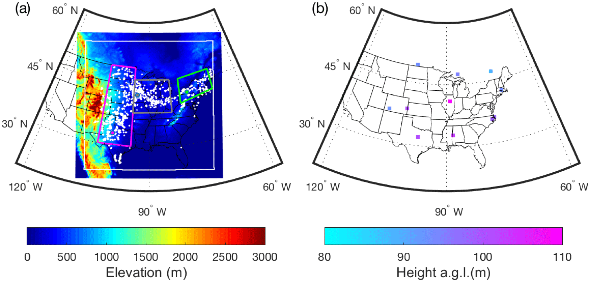
Figure 2(a) Simulation domain showing the terrain elevation in each of the total 101 761 grid cells, each of which is 12 km by 12 km. The white box denotes the edge of the adjustment zone applied and thus delimits the 78961 grid cells (281×281) that are considered herein. The overlaid white dots denote the grid cells in which there were one or more operating WTs as of March 2018. The sub-domains outlined in magenta, grey and green denote the areas referred to herein as the Central Plains, Midwest and Northeast, respectively. The magenta (TX), grey (IA) and green (NY) dots denote the grid cells used as illustrative examples of the simulated wind climate throughout (e.g., in the bootstrapping of the annual mean AEP and power spectral analyses). (b) Mean height of the third model layer above the local grid cell average model elevation for 10 sample locations across the simulation domain.
The time step used for the simulations is 72 s, and there are 41 vertical levels (in sigma hydrostatic pressure coordinate) up to a model top at 50 hPa. A total of 18 of those levels are below 1 km and the lowest 10 levels represent approximate heights (in flat terrain) of 16.7, 50.1, 83.6, 117, 151, 184, 218, 253, 293 and 338 m a.g.l. Wind speeds used herein are derived from the third model layer that represents a height above the ground in flat terrain at mean sea level of approximately 83 m. Variations in the actual height above the local terrain of this layer (Fig. 2b) arise primarily due to topographic variability such as the very high and steep complex terrain of the Rocky Mountains in the west of the simulation domain (where the sigma levels are compressed near the surface). The following physics schemes are employed. Numbering is as in the WRF namelist file.
-
Longwave radiation: 1. rapid radiative transfer model (RRTM; Mlawer et al., 1997)
-
Shortwave radiation: 1. Dudhia (Dudhia, 1989)
-
Microphysics: 5. Eta model (Ferrier et al., 2002)
-
Surface-layer physics: 1. MM5 similarity scheme (Beljaars, 1995)
-
Land surface physics: 2. Noah land surface model (Tewari et al., 2004)
-
Planetary boundary layer: 5. Mellor–Yamada–Nakanishi–Niino 2.5 (Nakanishi and Niino, 2006)
-
Cumulus parameterization: 1. Kain–Fritsch (Kain, 2004)
The simulations start on 15 February 2001 (on the first date for which RTG-SSTs are available) and run through the end of 31 December 2016. Analyses conducted herein are based on output from 1 March 2011 to 31 December 2016 to allow for a 14-day “spin-up”. The period required for “convergence” of interannual variability estimates of annual mean wind speed was previously evaluated by computing the standard deviation of mean annual wind speeds using output from a reanalysis data set of 35 years and comparing that estimate with the estimate derived from truncated samples thereof. That study found σ converges on the long-term estimate to within ±15 % after 11 years (Pullinger et al., 2017), which implies that the simulations presented herein are of sufficient duration to adequately characterize IAV.
Multiple factors impact the IAV of net AEP from operating wind farms, including but not limited to curtailment for system operation and/or WT maintenance (Clifton et al., 2016), WT wake losses (Clifton et al., 2016; Barthelmie et al., 2013) and wind speed variability. Here we focus on this last factor.
2.2 Estimating WI and AEP
Annual mean wind speeds are computed for each grid cell as the arithmetic mean of all 10 min output from the third model layer in each model grid cell. Wind indices (WIs) are computed by applying Eq. (1) to the same WRF output and using a reference time period of 2002–2016. The USGS database of the locations and types of all WTs deployed in the continental USA as of March 2018 indicates that 57 636 WTs were installed in the contiguous USA, of which three-quarters fall within the simulation domain (see Fig. 2a for the locations). The most common WT is a variant of the GE 1.5 SLE that has a hub height (HH) of 80 m, a rotor diameter (D) of 77 m and a rated capacity (RC) of 1.5 MW. Thus, WRF output is post-processed to generate a first-order estimate of AEP in each grid cell by assuming there is a single WT deployed in the center of each WRF grid cell and applying the power curve of a GE 1.5 SLE (Fig. 1) to 10 min wind speeds from the third model level.
2.3 Statistical methods
Output from three example grid cells (located in Texas (TX), Iowa (IA) and New York state (NY); see Fig. 2a) is used throughout to provide illustrative examples of the simulated wind climate. Time series of 10 min output from the third model layer for each calendar year in these grid cells are fitted to Weibull distributions using maximum likelihood methods (Pryor et al., 2004) wherein the probability of a wind speed of a given magnitude is given by
where A is the scale parameter and k is the shape parameter.
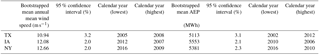
The results are used to demonstrate the year-to-year variability in the probability distribution parameters. These time series from each calendar year are also used with the power curve from the GE 1.5 MW WT to generate empirical estimates of the contribution of wind speed bins to the overall estimated power production in each year. Output from these grid cells over the entire period from 1 January 2002 to 31 December 2016 is also used to illustrate the temporal scales of variability in the entire sample using fast Fourier transform (FFT) applied to compute the variance across a range of frequencies and to present power spectra in the range to 50 day−1. Lastly, time series from these grid cells are also used to consider the question “how long is long enough?” In other words, what duration of time series is sufficient to characterize the overall annual mean wind speed and AEP with a certain level of confidence? Time series of the annual mean wind speed and AEP from the three grid cells highlighted in Fig. 2a (TX, IA and NY) are subject to a bootstrap analysis (Wilks, 2011) in which the annual mean wind speed and AEP estimates are resampled (with replacement) to generate a synthetic resampled data set of 1000 samples. These are used to compute an estimate of 95 % confidence intervals on the long-term mean wind speed AEP and identify the calendar years that differ most profoundly from the bootstrapped mean values in those three locations (Table 2).
Table 2Bootstrapped estimates of the mean wind speed in the third model layer and mean annual energy production (AEP); the associated 95 % confidence interval (i.e., expressed as a percent of the bootstrapped mean values ( Also shown are the years that fall furthest from the bootstrapped mean wind speed and AEP values (highest and lowest) for the three grid cells shown in Fig. 2a. Note: AEP is computed by assuming a single GE 1.5 MW WT is deployed in each 12 km×12 km grid cell and by applying the power curve of that WT to 10 min output from the WRF model.
Although it is common practice to describe the IAV of annual wind speeds using a standard deviation around the mean, the assumption that the samples of annual mean wind speed conform to a Gaussian distribution is not always evaluated. The distributions of the 15 values of annual mean wind speed, WI and AEP from each grid cell considered herein are not normally distributed, rendering the mean and standard deviation poor descriptors of both the central tendency and the dispersion around the central tendency. Indeed, the samples of 15 annual mean wind speed and AEP estimates fail the Anderson–Darling test for normalcy (Wilks, 2011) in 97.7 % and 96.3 % of grid cells (for a 95 % confidence level). Thus, herein we describe the central tendency using the median value (P50) and use the interquartile range (IQR; i.e., 25th to 75th percentile range) to describe the dispersion. We also derive estimates of the 90 % intervals around the median annual mean wind speed and AEP (i.e., the range within which 9 out of 10 years are expected to fall), but emphasize that these are based on a very small sample size (of 15) and thus are subject to relatively large uncertainty. They are presented solely to permit comparison with 90 % intervals around the mean computed using 1.645σ (for normally distributed variables; Wilks, 2011) applied to past literature that has stated variability in terms of the standard deviation around the mean (Table 1).
P50(AEP) and P90(AEP) are computed for individual calendar years and for rolling consecutive 12-month periods. In the former, 10 min output wind speeds from all grid cells for each of the 15 full calendar years (i.e., 2002, 2003 etc.) are subject to the WT power curve and used to compute AEP for each calendar year. In the latter, 10 min output wind speeds from all grid cells for rolling 12-month periods (i.e., March 2001 to February 2002, April 2001 to March 2002) are subject to the WT power curve and used to compute AEP for all consecutive 12-month periods. Output from the rolling 12-month periods is used to identify the 12-month period with the highest and lowest AEP, and those values are evaluated spatially to examine the degree to which that time index and hence the timing of periods with the highest and lowest AEP are spatially coherent. The results are considered in the context of monthly indices of the phase of three important internal climate modes that have previously been shown to influence the intra-annual and interannual variability of wind speeds over the USA (Schoof and Pryor, 2014; Pryor and Ledolter, 2010): the Pacific North American (PNA) (Leathers et al., 1991), North Atlantic Oscillation (NAO) (Hurrell et al., 2003) and Niño Oceanic Index (ONI), which is a 3-month running mean of sea surface temperature anomalies in the Niño 3.4 region (Ren and Jin, 2011).
The mean gross capacity factor (CF) for each grid cell is computed as the amount of electrical power produced in each calendar year by applying the power curve for the GE 1.5 MW machine to output from each 10 min period and comparing the result to the maximum possible as determined by the rated capacity (1.5 MW) multiplied by the number of hours in a year.
The 1612 of the 281×281 (i.e., 78 961) total grid cells (with adjustment zone removed) that contain operating WTs as of March 2018 are the primary focus of the analyses presented herein (and are referred to as WT grids). Results are also compared to output from the other grid cells (without WTs, referred to herein as “no”) to determine whether areas that currently have WTs deployed in them exhibit higher or lower interannual variability than typifies the study domain.
2.4 Observational data
There are a number of “bottlenecks” to improved estimation of IAV in mean wind speeds at WT relevant heights and in AEP from WTs. These include the lack of publicly accessible high-accuracy data at WT relevant heights and high temporal resolution for the evaluation of numerical simulations such as those presented herein (Kusiak, 2016). The National Weather Service (NWS) operates over 900 stations where wind speeds are measured at a height of 10 m a.g.l., but these data are not at or close to WT hub heights and the actual vertical profile of wind speed is strongly dependent on stability, making vertical extrapolation highly uncertain (Badger et al., 2016; Barthelmie et al., 1993; Motta et al., 2005). Additionally, wind speeds as measured by 2-D sonic anemometers at NWS stations are recorded at a resolution of 1 knot (0.514 m s−1) rounded up to the nearest knot when they are archived. The resulting sample is thus systematically biased and pseudo-categorical. Further, in terms of model validation, local topography and obstacles greatly impact near-surface observations of wind speeds, which makes comparison with grid cell mean values as derived from a numerical model challenging. For these and other reasons, herein we contextualize the results of our numerical simulations using observationally derived estimates of the IAV of annual net power production from operating wind farms. Power production data for nearly 1000 operating wind farms as obtained from the US Energy Information Administration (EIA) (downloaded from https://www.eia.gov/electricity/data/eia923/, last access: 4 June 2018) are used to estimate monthly capacity factors for each calendar month; January 2001 to December 2016. Sites with ≥9 years of data with ≥9 months of data availability in each year are used to compute the median annual mean net CF and the normalized IAV therein as represented by the interquartile range of annual net CF divided by the median net CF (IQR(CF) ∕ P50(CF)). A total of 68 sites meet this data completeness criterion. It is important to note that the application of these selection criteria is necessary to ensure that the resulting IQRs in CF estimates are robust, but it biases the resulting sample in two important ways: the overwhelming majority of these wind farms are located in the Central Plains (Fig. 3b) and they tend to represent older-generation wind farms in which WTs may no longer be under warranty and may experience declining performance (Olauson et al., 2017), potentially leading to inflation of the IAV(CF).
3.1 Wind speed variability
Median annual mean wind speeds from the third model level exhibit the expected spatial variability with the highest wind speeds over the Central Plains and in a swath across the upper Midwest into the northeastern states (Fig. 3a). This is consistent with the placement of WTs in the domain (Fig. 2a) and previous resource assessments (Pryor and Barthelmie, 2011; U.S. Department of Energy, 2015; Clifton et al., 2018). Annual gross capacity factors (CFs) for grid cells with WTs currently deployed in them (WT grid) as derived from the approximations used herein are also consistent with direct observations. The median gross CF computed herein is 40.4 % (Fig. 3d), which is higher than the net CF derived from the 68 operating wind farms (shown in Fig. 3c) of 36 % and slightly lower than the value of 42.5 % for WT installations commissioned in 2016 (Wiser and Bolinger, 2017). The median gross CF computed herein for WT grids is higher than the observed net CF from the 68 operating wind farms because the net CF also incorporates reductions in power production due to WT maintenance activities, wind turbine wake effects and curtailment for grid management. Observed levels of curtailment over much of the study domain considered herein were ≤4 % during 2007–2012 (Bird et al., 2014). Wind power plant efficiency reductions due to wind turbine wakes are known to be smaller in onshore wind farms than those offshore due to the irregular layouts, higher ambient turbulence intensity and the typically smaller wind turbine densities. Typical wind-turbine-induced wakes losses for onshore wind farms are often estimated to be ≤5 % (Staid et al., 2018), while those offshore are frequently in excess of 10 % (Barthelmie et al., 2013). Onshore availability typically exceeds 98 % (Carroll et al., 2017), but tends to decrease with WT age (Olauson et al., 2017). Thus gross CF derived from the WRF simulations that assume 100 % WT availability (i.e., no downtime for maintenance or curtailment of production) and no wake losses is inevitably higher than the observed values derived from wind farms that have been in operation for more than 10 years. The estimated median CFs derived herein are lower than observed values for new WT deployments in 2016 because the newer WTs that are currently being installed have higher WT hub heights and larger rotors and RCs than the GE 1.5 MW WT applied herein.
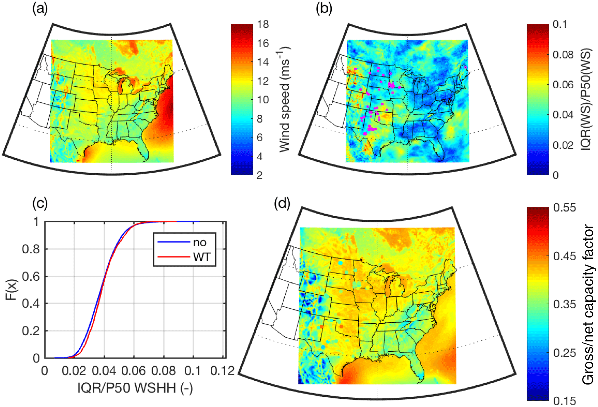
Figure 3(a) Median (i.e., P50) of annual mean wind speeds in the third model layer of each 12 km×12 km grid cell as derived from 10 min output. (b) The normalized interquartile range of annual mean wind speeds (IQR(WS) ∕ P50(WS)). The magenta dots shown in this frame denote the locations of operating wind farms from which median CFs are shown in (d). (c) Cumulative density function of IQR(WS) ∕ P50(WS) in the sample of grid cells containing WTs (shown as WT in the legend) and those that do not (shown as “no” in the legend). (d) Median annual gross capacity factors (CFs) for a single WT deployed in each 12 km×12 km grid cell derived using 10 min output from the WRF model and the power curve from a GE 1.5 MW WT (see Fig. 1). Also shown by the dots in (d) is the median net CF computed directly from the power output of operating wind farms. The same color scale is used for the gross (simulated) and net (observed) CF. If the net and gross capacity factors are equal the wind farm locations (shown in b) will not be visible, implying agreement between observed and simulated values.
Output for each calendar year from the three grid cells (in Texas (TX), Iowa (IA) and New York (NY); see Fig. 2a for locations) conforms to two-parameter Weibull distributions as indicated by narrow 95 % confidence intervals around the distribution parameters and also illustrate relatively high consistency across the calendar years (Fig. 4a). The fraction of power production from each wind speed bin (also plotted in Fig. 4a) highlights the fact that the variability of the tail of the wind speed distribution dominates IAV in power production rather than values below the annual mean. Indeed, wind speeds in excess of the annual mean contribute an average of 69 %, 66 % and 57 % of the estimated annual total power production in these grid cells from TX, IA and NY. This emphasizes important potential disconnects between the variability of the annual mean wind speed and AEP. The bootstrapped estimate of the annual mean wind speed (and 95 % confidence intervals based thereon) in the illustrative grid cells from TX, IA and NY state fall at a place on the power curve that is relatively close to the wind speed at which the GE 1.5 MW WT generates rated power (i.e., the power output ceases to increase with increasing wind speeds). This implies that small changes in annual mean wind speeds may not greatly impact the cumulative power output.
Analyses of time series of 10 min output from these three grid cells in the frequency domain indicate that in all of these grid cells the variance is dominated by the meso-α to synoptic timescale (f≈0.2–0.5 day−1, thus periods of 2–5 days) (Fig. 4b). There is also a clear diurnal peak, particularly in IA and NY, while in TX this local maximum is displaced to periods slightly shorter than 1 day. Power spectra derived from output from all three grid cells also exhibit maxima in the frequency range 2 to day−1 (i.e., on annual timescales). This timescale exhibits the greatest magnitude of variance in the grid cell from New York state and is of lowest magnitude in Iowa. Variability across all these timescales contributes to the variations in power output from WTs, the resulting AEP, and thus both P50(AEP) and P90(AEP). Although the power spectra of wind speeds exhibit a height dependence in the planetary boundary layer and due to the parameterizations used mesoscale model simulations are deficit in high-frequency variability (Larsén et al., 2012, 2016), Fig. 4b further reemphasizes the motivation for this research. As shown, the variance at virtually all frequencies considered herein is highest in output from the NY grid cell. This inevitably leads to the question of whether the use of a constant factor to represent IAV (as in work that has used σ=6 %) on annual mean wind speeds and/or AEP is appropriate everywhere.
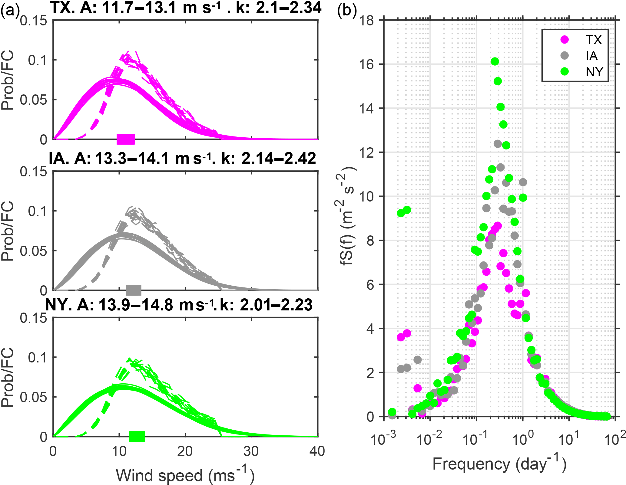
Figure 4(a) Weibull distributions calculated for each year for the third model level wind speeds (solid lines) for three example grid cells in Texas (TA), Iowa (IA) and New York (NY) state (see Fig. 2a for the locations of these grid cells). The dashed lines show empirical distributions of the contribution of wind speeds in 1 m s−1 bins to the overall annual energy production (FC). The solid colored boxes on the x axes indicate the range of mean annual wind speeds in each grid cell. The Weibull parameters for each site are shown above each frame. A is the Weibull scale factor (in m s−1) and k is the shape factor. (b) Power spectra of 10 min disjunct horizontal wind speeds from the third model level from each of these grid cells computed using output every 10 min for 1 January 2002 to 31 December 2016.
The normalized IQR of annual mean wind speeds (IQR(WS) ∕ P50(WS)) is <4 % in nearly 60 % of WT grid cells, <5 % in 83 % of WT grid cells and <6 % in 96 % of WT grid cells (Fig. 3b and c; see summary in Table 1). Recall that a large IQR(X) ∕ P50(X) indicates a site or area with high IAV in parameter X. Thus, this analysis indicates that in 5 out of 10 years the annual mean wind speed will fall within ±4 % of the long-term average in 90 % of the simulation grid cells that contain operating wind turbines. The estimated 90 % confidence interval around the median annual mean wind speed (i.e., 5th to 95th percentile span in values divided by the median, P50) is <8 % in half of all WT grid cells and <11 % in 90 % of WT grid cells. Thus, this implies that in 9 out of 10 years the annual mean wind speed is expected to fall within ±5.5 % of the long-term average in 90 % of the simulation grid cells that contain currently operating wind turbines. Comparative estimates of the range of expected annual mean wind speeds derived assuming a Gaussian distribution and σ of 6 % are considerably larger. They yield 90 % confidence intervals around of mean that span 19 % (i.e., in 9 out of 10 years the annual mean wind speed is expected to fall within ±10 % of the long-term average). Several grid cells in the Southern Great Plains indicate higher IQR(WS) ∕ P50(WS) than the median value of 3.8 %. However, the lowest 50 % of IQR(WS) ∕ P50(WS) of annual mean wind speeds in WT cells is lower than in grid cells without WTs. This indicates that, on average, the locations at which WTs are currently operating are characterized by lower IAV in wind speeds than typifies the eastern half of North America.
3.2 Wind indices and AEP
The spatial mean P90(AEP) from WT grid cells is 5157 MWh yr−1, while P50(AEP) is 5323 MWh yr−1 (Figs. 5c, d and 6). Comparable figures from grid cells that do not contain the locations of currently operating WTs (i.e., no WT grid) are 4893 and 5078 MWh yr−1, indicating that WTs are deployed in locations that have atypically high wind speeds and projected AEP.
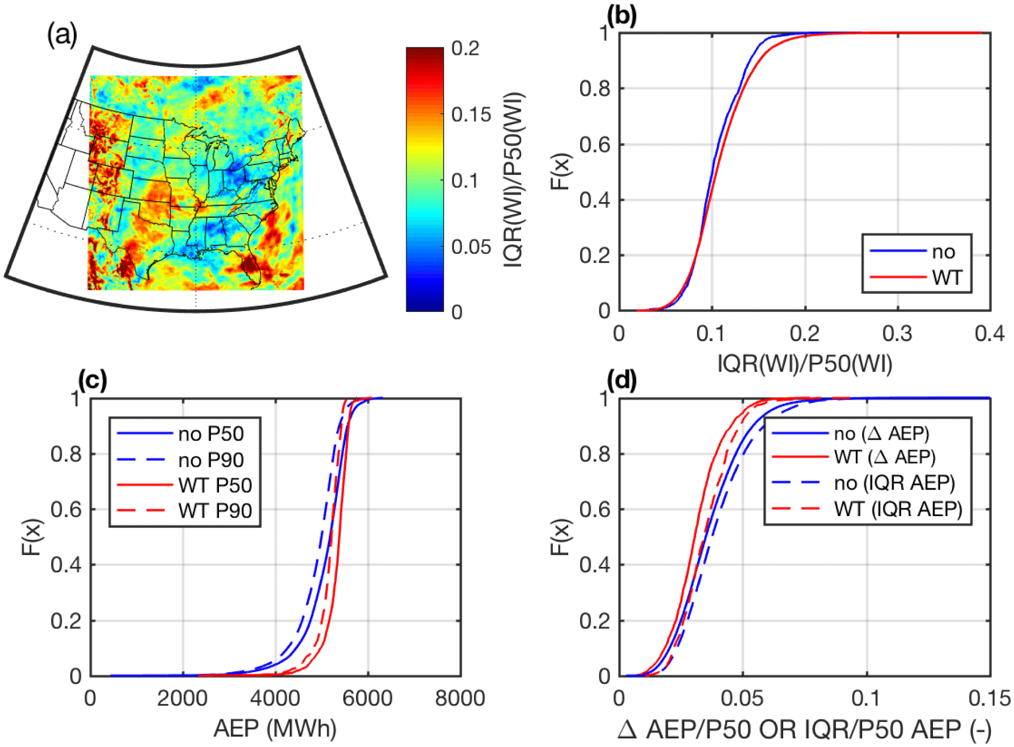
Figure 5(a) Spatial map of normalized IQR wind index and (b) cumulative density plot of the normalized IQR wind index in a sample of grid cells containing WTs (WT) and those that do not (“no”). Cumulative density plots of (c) P50(AEP) and P90(AEP) (in MWh) and the (d) normalized difference between AEP P50, P90 (i.e., and IQR(AEP) ∕ P50(AEP) in the sample of grid cells containing WTs (WT) and those that do not (“no”). AEP is computed by assuming a single GE 1.5 MW WT is deployed in each 12 km×12 km grid cell and by applying the power curve of that WT to 10 min output from the WRF model.
WIs (computed using Eq. 1) naturally exhibit larger normalized IQR than annual mean wind speeds (cf. Figs. 5a and 3b). Normalized IQR of WI (IQR(WI) ∕ P50(WI)) is <11 % in 60 % of WT grid cells, <14 % in 83 % of WT grid cells and <15 % in 95 % of WT grid cells (Fig. 5b; see summary in Table 1). However, a similar inflation of IAV is not anticipated for AEP because of the nature of wind turbine power curves (see example in Fig. 1). This expectation is realized within the estimated AEP values. The spatial median value of normalized IQR of AEP (i.e., IQR(AEP) ∕ P50(AEP)) is 3.4 %, and thus half of all years are estimated to fall within ±3.4 % of the median (P50) AEP for half of all WT grid cells. The 90 % confidence interval tentatively derived as the 5th to 95th percentile of annual median AEP in each grid cell indicates that WT grid cells range from 5.0 % to 13.5 % with a median of 7.9 %. Thus, in half of all simulation grid cells that cover areas where WTs are currently operating, in 9 out of 10 years AEP is expected to fall within ±4 % of the long-term average (Table 1). Comparative estimates of the range of expected AEP derived assuming a Gaussian distribution and σ of 6 % are considerably larger and yield 90 % confidence intervals around the mean that span 19 % (i.e., in 9 out of 10 years the AEP is expected to fall within ±10 % of the long-term average). Thus, it would appear that assuming a standard deviation (σ) of 6 % for the climate-induced interannual variability in AEP is conservative and potentially could be reduced. Under the assumption that the WTs deployed are GE 1.5 SLE and that they are harvesting wind speeds at a height equal to the third model layer, the normalized difference between P90(AEP) and P50(AEP) in WT grid cells is <3.1 % in 50 % of grid cells and is below 4.6 % in 90 % of WT grid cells (Figs. 5c and d and 6c). Indeed, only 1 % of WT grid cells exhibit values in excess of 6.4 %.
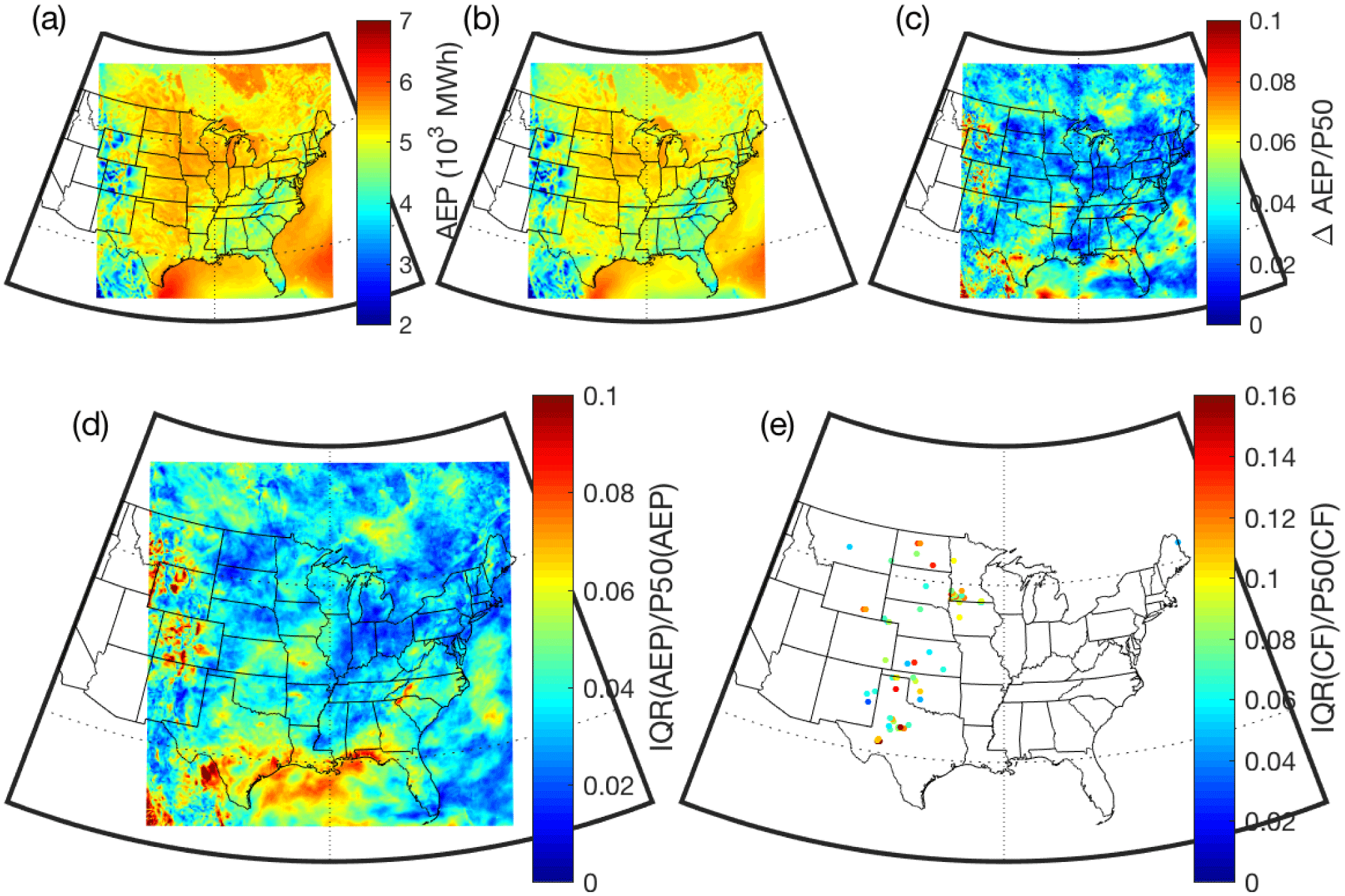
Figure 6(a) P50(AEP) and (b) P90(AEP) (in 103 MWh) from a single 1.5 MW WT in each 12 km×12 km grid cell derived using 10 min output from the WRF model and the power curve from a GE 1.5 MW WT. (c) The difference in P90 and P50 AEP expressed as a fraction of P50 AEP (ΔAEP ∕ P50(AEP)). (d) The normalized interquartile range of AEP (IQR(AEP) ∕ P50(AEP)) in each WRF grid cell and (e) the normalized interquartile range of mean annual capacity factor (IQR(CF) ∕ P50(CF)) from operating wind farms. Note: the scales in (d) and (e) differ in order to best depict the full range of values from each data set.
The mean normalized IQR of gross AEP as derived using output from the WRF simulations and the GE 1.5 MW power curve for grid cells containing the 68 operating wind farms considered herein is 3.5 % (Fig. 6d). The normalized IQR of net CF derived from power production data at these wind farms ranges from 3 % to 18 % and has a median value of 9 % (Fig. 6e). Thus, the power production data from these operating wind farms indicate that in half of them the production during half of all years lies within % of the long-term average (see summary in Table 1). Our simulations imply that the climate-induced variability at these locations is likely to mean that AEP in half of all years should lie within ±2 % of the long-term average, with the remaining variability being derived from other factors such as performance deductions due to WT aging, curtailment and maintenance. These estimates are tentative because the power production data sets are of short duration and contain missing data, and the model simulations are also only 15 years in duration and make a number of assumptions (including the use of a single WT power curve). Nevertheless this analysis highlights the need for further studies designed to decompose the IAV of AEP into the root causes of wind climate variability, curtailment, WT availability and WT performance degradation with age.
3.3 Scales of coherence in wind speed variability
Understanding the spatial scales of coherence at which wind speed variability on different timescales is manifest is important to the integration of wind-energy-generated electricity into the grid. Over much of the US, the variability of wind speeds on seasonal to interannual timescales is determined by the frequency and tracking of midlatitude cyclones as dictated by the phase of internal climate modes (Schoof and Pryor, 2014). The timing of the occurrence of the rolling 12-month period of minimum and maximum AEP as computed from the WRF simulations exhibits relatively complex spatial patterns (Fig. 7). This indicates that at least at the annual scale, the geographic dispersal of wind turbine deployments is such that it extends beyond regions of high coherence in gross AEP. However, there are also regions of coherence consistent with the importance of large-scale climate modes in dictating wind speed anomalies over the contiguous USA (Schoof and Pryor, 2014). Minimum AEP over the upper Midwest (i.e., over Minnesota, Michigan, Illinois, Indiana and Ohio) occurred during 2011 (and early 2012; Fig. 7a) during a weak La Niña period (i.e., negative ONI; see Fig. 7c), while in the lower Central Plains (Fig. 7a) the timing of this minimum was more strongly focused on 2015–2016 during a relatively strong El Niño event (i.e., positive ONI; Fig. 7c). Conversely, the upper Central Great Plains and parts of the southeast exhibit the lowest values for a 12-month period starting in mid-2008 (during a weak la Niña, Fig. 7). The timing of maximum AEP is also consistent across the upper Midwest states and is focused on 2007 (Fig. 7b). Much of the Central Plains indicate maximum AEP for a period centered on 2011, while estimated AEP in the northeastern states is highest close to the start of the simulation period in 2001–2002. Analysis of the years that differ most from the bootstrapped mean AEP from the three sample grid cells (IA, TX and NY; see Table 2) reemphasizes the findings of the analysis presented in Fig. 7. Both indicate that different regions within the eastern USA differ in terms of 12-month period that has the lowest AEP and thus when viewed system-wide (i.e., spatially) there are important compensating variations in the wind climate and derived AEP. For example, although 2010 is indicated as a year of relatively low electricity production in Iowa, it is associated with higher than average AEP from WTs in New York state. Figure 7 further illustrates that the IAV of AEP (and wind speeds) and the occurrence of higher than normal values is a complex function of the state of multiple climate modes (Schoof and Pryor, 2014). For example, late 2006 saw a weak positive ONI and positive PNA and NAO and was associated with relatively high AEP over much of the Midwest, but late 2009 when ONI was also positive but NAO was negative and PNA was closest to zero was not associated with high estimated AEP over the Midwest.

Figure 7Timing of the start of the (a) minimum and (b) maximum 12-month rolling AEP value in each 12 km×12 km grid cell derived using 10 min output from the WRF model and the power curve from a GE 1.5 MW WT. The white dots indicate the locations of operating WTs as of March 2018. As in Figs. 5 and 6 AEP is computed by assuming a single GE 1.5 MW WT is deployed in each 12 km×12 km grid cell and by applying the power curve of that WT to 10 min output from the WRF model. The panels on the right of each map denote the fraction of all grid cells (Frac) that exhibit a minimum or maximum 12-month rolling AEP in each 12-month period. For a random variable the expectation is that this fraction would be 0.0023 in each time period. (c) Monthly indices of the phase of the Pacific North American (PNA), North Atlantic Oscillation (NAO) and Oceanic Niño Index (ONI).
This study addresses a key aspect of uncertainty in wind project financing – the magnitude of the IAV of wind speeds as manifest in AEP. Over the eastern USA under the contemporary climate, the interannual variability of annual mean wind speeds close to typical wind turbine hub heights is smaller than implied by using a standard deviation of 6 %. While the IAV for wind indices is naturally higher than for wind speeds, the IAV of AEP is close to that derived for annual mean wind speeds (see Tables 1 and 2). The difference between P90(AEP) and P50(AEP) in 12 km×12 km simulation grid cells that currently contain WTs is generally below 5 % of P50(AEP) and is <10 % of P50(AEP) for the overwhelming majority of grid cells within the study domain and all grid cells that contain operating WTs. The analyses presented herein indicate that AEP in 9 out of 10 years will lie within ±5 % of the median value in 90 % of grid cells that cover areas that currently contain WTs. Thus, the use of a 6 % standard deviation to represent variability in pre-project estimated mean AEP variability due to contemporary climate variability would appear to be conservative over the overwhelming majority of the eastern USA. The 90 % confidence interval on AEP associated with σ=6 % is ±10 %. It may be more appropriate to assign σ∼4 % to account for climatological variability in the wind resource. However, we caution that implicit assumptions that mean wind speeds and AEP are Gaussian distributed are not warranted, and thus the dispersion (IAV) should not be characterized using parametric statistics such as the standard deviation. In pre-project financing for developments in the eastern half of North America, it may be more appropriate to assume that climatological variability is such that the annual mean wind speed and AEP in 9 out of 10 years will lie within ±6 % of the long-term mean.
Although climate modes (such as ENSO) exert an important control on wind regimes over the eastern USA and coherent sub-domains within the region exist in terms of the timing of the maximum and minimum estimated AEP, these regions of coherence are sufficiently small that, for example, there are compensating effects between Iowa and New York state. Thus, for a strong and well-connected distribution grid the interannual variability in AEP from wind turbines would be small. Indeed, for the current distributed WT network the interquartile range in system-wide AEP computed from the 15 annual total production estimates derived by equally weighting all grid cells with WTs in them is only slightly over 1 %.
Naturally, there are a number of caveats that should be applied to our findings. It is implicitly assumed herein that 2001–2016 is a representative climate period. The magnitude of the interannual variation in wind speeds, wind indices and AEP reported herein is a function of the simulation period (2001–2016), the lateral boundary conditions applied (ERA-Interim) to the simulations and the application of a single WT power curve to compute AEP. It is important to emphasize that simulated wind climate regimes are a function of the physics packages applied within WRF and the resolution at which the model is applied (Draxl et al., 2014); we further reiterate that the research presented herein neglects non-climatic factors that influence AEP such as curtailment for system operation and/or WT maintenance and IAV in reduced power production efficiency of wind farms (due to wake loss variability resulting from changes in the prevailing wind direction). Herein we assume that these effects are secondary to variations in the magnitude of wind speeds. Future work should address the validity of this and the other assumptions employed herein.
This study indicates the urgent need for further research to reduce uncertainty in climate-induced IAV in AEP. Our research suggests the actual IAV in WT-generated electricity (AEP) over the eastern USA may be substantially below the levels that are currently adopted in financing mechanisms within the industry. This finding implies that the cost of capital for wind projects may be too high.
The USGS Wind Turbine Database is available for download from https://eerscmap.usgs.gov/uswtdb/ (last access: 4 June 2018). Monthly values of the Pacific North American, North Atlantic Oscillation and Niño Oceanic Index are available from the NOAA Climate Prediction Center (https://www.esrl.noaa.gov/psd/data/climateindices/list/, last access: 4 June 2018). Power production data for nearly 1000 operating wind farms are available from the US Energy Information Administration (EIA; https://www.eia.gov/electricity/data/eia923/, last access: 4 June 2018). Netcdf files containing the derived variables from our WRF output that underpin each of the analyses and figures presented herein are accessible via the Zenodo repository (Pryor et al., 2018).
SCP and RJB conceived the original concept and obtained the funding for the research. SCP conducted the analyses of the WRF output presented here and drafted the initial paper and all figures. RJB and SCP formulated the scenarios employed and the statistical methodology. TJS performed the WRF simulations. All authors jointly finalized the paper.
The authors declare that they have no conflict of interest.
This research was funded by the US Department of Energy (DE-SC0016438) and
Cornell University's Atkinson Center for a Sustainable Future
(ACSF-sp2279-2016). This research was enabled by access to a range of
computational resources supported by the NSF (ACI-1541215 and those made
available via the NSF Extreme Science and Engineering Discovery Environment, XSEDE; award TG-ATM170024)
and those of the National Energy Research
Scientific Computing Center, a DOE Office of Science user facility supported
by the Office of Science of the US Department of Energy under contract no. DE-AC02-05CH11231.
The authors gratefully acknowledge stimulating
conversations with Ken Westrick and Ken Davies, the work of Peter Cook in
undertaking initial processing of the EIA data, and Brandon Barker and
Bennett Wineholt for maintaining the Aristotle cloud system. We also
gratefully acknowledge the many people who have contributed to the
development of the WRF model and the two reviewers who provided helpful feedback
on our original submission.
Edited by: Joachim Peinke
Reviewed by: David Pullinger and one anonymous referee
Badger, M., Peña, A., Hahmann, A. N., Mouche, A. A., and Hasager, C. B.: Extrapolating satellite winds to turbine operating heights, J. Appl. Meteorol. Clim., 55, 975–991, 2016.
Barthelmie, R. J., Palutikof, J. P., and Davies, T. D.: Estimation of sector roughness and the effect on prediction of the vertical wind speed profile, Bound.-Lay. Meteorol., 66, 19–47, 1993.
Barthelmie, R. J., Murray, F., and Pryor, S. C.: The economic benefit of short-term forecasting for wind energy in the UK electricity market, Energ. Policy, 36, 1687–1696, 2008.
Barthelmie, R. J., Hansen, K. S., and Pryor, S. C.: Meteorological controls on wind turbine wakes, Proc. IEEE, 101, 1010–1019, 2013.
Beljaars, A.: The parametrization of surface fluxes in largescale models under free convection, Q. J. Roy. Meteor. Soc., 121, 255–270, 1995.
Bett, P. E., Thornton, H. E., and Clark, R. T.: Using the Twentieth Century Reanalysis to assess climate variability for the European wind industry, Theor. Appl. Climatol., 127, 61–80, 2017.
Bird, L., Cochran, J., and Wang, X.: Wind and solar energy curtailment: Experience and practices in the United States, National Renewable Energy Laboratory, Colorado, available at: https://www.nrel.gov/docs/fy14osti/60983.pdf (last access: 4 June 2018), 58, 2014.
Blanco, M. I.: The economics of wind energy, Renewable and Sustainable Energy Reviews, 13, 1372–1382, 2009.
Brower, M. C.: Wind Resource Assessment: A Practical Guide to Developing a Wind Project, John Wiley & Sons, Inc., Hoboken, New Jersey, 280 pp., 2012.
Carroll, J., McDonald, A., Dinwoodie, I., McMillan, D., Revie, M., and Lazakis, I.: Availability, operation and maintenance costs of offshore wind turbines with different drive train configurations, Wind Energy, 20, 361–378, 2017.
Clifton, A., Smith, A., and Fields, M.: Wind Plant Preconstruction Energy Estimates. Current Practice and Opportunities, National Renewable Energy Lab.(NREL), Golden, CO (United States), NREL/TP-5000-64735. National Renewable Energy Laboratory (NREL), Golden, CO (US), available at: http://www.nrel.gov/docs/fy16osti/64735.pdf (last access: 4 June 2018), 2016.
Clifton, A., Hodge, B. M., Draxl, C., Badger, J., and Habte, A.: Wind and solar resource data sets, Wires. Energy Environ., 7, e276, https://doi.org/10.1002/wene.276, 2018.
Danielson, J. J. and Gesch, D. B.: Global multi-resolution terrain elevation data 2010 (GMTED2010), U.S. Geological Survey Open-File Report 2011–1073, available at: https://pubs.usgs.gov/of/2011/1073/pdf/of2011-1073.pdf (last access: 4 June 2018), 26, 2011.
Dee, D. P., Uppala, S., Simmons, A., Berrisford, P., Poli, P., Kobayashi, S., Andrae, U., Balmaseda, M., Balsamo, G., and Bauer, P.: The ERAInterim reanalysis: Configuration and performance of the data assimilation system, Q. J. Roy. Meteor. Soc., 137, 553–597, 2011.
Dowell, J. and Pinson, P.: Very-short-term probabilistic wind power forecasts by sparse vector autoregression, IEEE T. Smart Grid, 7, 763–770, 2016.
Draxl, C., Hahmann, A. N., Peña, A., and Giebel, G.: Evaluating winds and vertical wind shear from Weather Research and Forecasting model forecasts using seven planetary boundary layer schemes, Wind Energy, 17, 39–55, 2014.
Dudhia, J.: Numerical study of convection observed during the winter monsoon experiment using a mesoscale two-dimensional model, J. Atmos. Sci., 46, 3077–3107, 1989.
Dykes, K., Hand, M., Stehly, T., Veers, P., Robinson, M., Lantz, E., and Tusing, R.: Enabling the SMART Wind Power Plant of the Future Through Science-Based Innovation, NREL/TP-5000-68123, National Renewable Energy Laboratory, CO, available at: https://www.nrel.gov/docs/fy17osti/68123.pdf (last access: 4 June 2018), 57, 2017.
Feldman, D. and Bolinger, M.: On the Path to SunShot: Emerging Opportunities and Challenges in Financing Solar, National Renewable Energy Laboratory, Golden, CO, NREL/TP-6A20-65638, available at: http://www.nrel.gov/docs/fy16osti/65638.pdf (last access: 4 June 2018), 109, 2016.
Ferrier, B. S., Jin, Y., Lin, Y., Black, T., Rogers, E., and DiMego, G.: Implementation of a new grid-scale cloud and precipitation scheme in the NCEP Eta model, 15th Conf. on Numerical Weather Prediction, 280–283, 2002.
Friedl, M. A., Sulla-Menashe, D., Tan, B., Schneider, A., Ramankutty, N., Sibley, A., and Huang, X.: MODIS Collection 5 global land cover: Algorithm refinements and characterization of new datasets, Remote Sens. Environ., 114, 168–182, https://doi.org/10.1016/j.rse.2009.08.016, 2010.
Früh, W.-G.: Long-term wind resource and uncertainty estimation using wind records from Scotland as example, Renew. Energ., 50, 1014–1026, https://doi.org/10.1016/j.renene.2012.08.047, 2013.
Gatzert, N. and Kosub, T.: Risks and risk management of renewable energy projects: The case of onshore and offshore wind parks, Renewable and Sustainable Energy Reviews, 60, 982–998, https://doi.org/10.1016/j.rser.2016.01.103, 2016.
Gemmill, W., Katz, B., and Li, X.: Daily real-time, global sea surface temperature – High-resolution analysis: RTG_SST_HR, NCEP, EMC Tech. Rep., 260, 39, available at: http://polar.ncep.noaa.gov/mmab/papers/tn260/MMAB260.pdf (last access: 4 June 2018), 2007.
Hamlington, B., Hamlington, P., Collins, S., Alexander, S., and Kim, K. Y.: Effects of climate oscillations on wind resource variability in the United States, Geophys. Res. Lett., 42, 145–152, 2015.
Hurrell, J. W., Kushnir, Y., Ottersen, G., and Visbeck, M.: An overview of the North Atlantic Oscillation, in: The North Atlantic Oscillation: climatic significance and environmental impact, edited by: Hurrell, J. W., Kushnir, Y., Ottersen, G., and Visbeck, M., AGU Geophysical Monograph Series, 1–35, 2003.
Kain, J. S.: The Kain–Fritsch convective parameterization: an update, J. Appl. Meteorol., 43, 170–181, 2004.
KirchnerBossi, N., GarcíaHerrera, R., Prieto, L., and Trigo, R.: A longterm perspective of wind power output variability, Int. J. Climatol., 35, 2635–2646, 2015.
Krupa, J. and Harvey, L. D. D.: Renewable electricity finance in the United States: A state-of-the-art review, Energy, 135, 913–929, https://doi.org/10.1016/j.energy.2017.05.190, 2017.
Kusiak, A.: Share data on wind energy: giving researchers access to information on turbine performance would allow wind farms to be optimized through data mining, Nature, 529, 19–22, 2016.
Lantz, E., Wiser, R., and Hand, M.: The past and future cost of wind energy, National Renewable Energy Laboratory, Golden, CO, Report No. NREL/TP-6A20-53510, available at: https://www.nrel.gov/docs/fy12osti/54526.pdf (last access: 4 June 2018), 2012.
Larsén, X. G., Ott, S., Badger, J., Hahmann, A. N., and Mann, J.: Recipes for correcting the impact of effective mesoscale resolution on the estimation of extreme winds, J. Appl. Meteorol. Clim., 51, 521–533, 2012.
Larsén, X. G., Larsen, S. E., and Petersen, E. L.: Full-scale spectrum of boundary-layer winds, Bound.-Lay. Meteorol., 159, 349–371, 2016.
Leathers, D. J., Yarnal, B., and Palecki, M. A.: The Pacific/North American Teleconnection pattern and the United State Climate. Part I: regional temperature and precipitation associations, J. Climate, 4, 517–528, 1991.
Mlawer, E. J., Taubman, S. J., Brown, P. D., Iacono, M. J., and Clough, S. A.: Radiative transfer for inhomogeneous atmospheres: RRTM, a validated correlatedk model for the longwave, J. Geophys. Res.-Atmos., 102, 16663–16682, 1997.
Motta, M., Barthelmie, R. J., and Vølund, P.: The influence of non-logarithmic wind speed profiles on potential power output at Danish offshore sites, Wind Energy, 8, 219–236, 2005.
Nakanishi, M. and Niino, H.: An improved Mellor–Yamada level-3 model: Its numerical stability and application to a regional prediction of advection fog, Bound.-Lay. Meteorol., 119, 397–407, 2006.
Olauson, J., Edström, P., and Rydén, J.: Wind turbine performance decline in Sweden, Wind Energy, 20, 2049–2053, 2017.
Orwig, K. D., Ahlstrom, M. L., Banunarayanan, V., Sharp, J., Wilczak, J. M., Freedman, J., Haupt, S. E., Cline, J., Bartholomy, O., and Hamann, H. F.: Recent trends in variable generation forecasting and its value to the power system, IEEE T. Sustain. Energ., 6, 924–933, 2015.
Pinson, P., Chevallier, C., and Kariniotakis, G. N.: Trading wind generation from short-term probabilistic forecasts of wind power, Power Systems, IEEE T., 22, 1148–1156, 2007.
Pryor, S. C. and Barthelmie, R. J.: Climate change impacts on wind energy: A review, Renewable and Sustainable Energy Reviews, 14, 430–437, 2010.
Pryor, S. C. and Barthelmie, R. J.: Assessing climate change impacts on the near-term stability of the wind energy resource over the USA, P. Natl. Acad. Sci. USA, 108, 8167–8171, 2011.
Pryor, S. C. and Ledolter, J.: Addendum to: Wind speed trends over the contiguous USA, J. Geophys. Res., 115, D10103, https://doi.org/10.1029/2009JD013281, 2010.
Pryor, S. C., Nielsen, M., Barthelmie, R. J., and Mann, J.: Can satellite sampling of offshore wind speeds realistically represent wind speed distributions? Part II: Quantifying uncertainties associated with sampling strategy and distribution fitting methods, J. Appl. Meteorol., 43, 739–750, 2004.
Pryor, S. C., Barthelmie, R. J., and Schoof, J. T.: Inter-annual variability of wind indices across Europe, Wind Energy, 9, 27–38, 2006.
Pryor, S. C., Barthelmie, R. J., Clausen, N., Drews, M., MacKellar, N., and Kjellström, E.: Analyses of possible changes in intense and extreme wind speeds over northern Europe under climate change scenarios, Clim. Dynam., 38, 189–208, 2012a.
Pryor, S. C., Barthelmie, R. J., and Schoof, J. T.: Past and future wind climates over the contiguous USA based on the NARCCAP model suite, J. Geophys. Res., 117, D19119, https://doi.org/10.1029/2012JD017449, 2012b.
Pryor, S. C., Barthelmie, R. J., and Shepherd, T. J.: WRF output. Resolution: 12 km. Domain: Eastern North America, https://doi.org/10.5281/zenodo.1257144, 2018.
Pullinger, D., Zhang, M., Hill, N., and Crutchley, T.: Improving uncertainty estimates: Inter-annual variability in Ireland, J. Phys. Conf. Ser., 926, 012006, available at: http://iopscience.iop.org/article/10.1088/1742-6596/926/1/012006/pdf, 2017.
Raftery, P., Tindal, A., and Garrad, A.: Understanding the risks of financing wind farms, in: Proceedings of the 1997 European Wind Energy Conference, Dublin, Ireland, Irish Wind Energy Association, Dublin, Ireland, 77–81, 1998.
Raftery, P., Tindal, A., Wallenstein, M., Johns, J., Warren, B., and Vaz, F.: Understanding the risks of financing wind farms, in: Proceedings of the 1999 European Wind Energy Conference: Wind Energy for the Next Millennium, edited by: Petersen, E. L., 496–499, 1999.
Ren, H. L. and Jin, F. F.: Niño indices for two types of ENSO, Geophys. Res. Lett., 38, L04704, https://doi.org/10.1029/2010GL046031, 2011.
Schoof, J. T. and Pryor, S. C.: Assessing the fidelity of AOGCMsimulated relationships between largescale modes of climate variability and wind speeds, J. Geophys. Res., 119, 9719–9734, 2014.
Sperati, S., Alessandrini, S., Pinson, P., and Kariniotakis, G.: The “Weather Intelligence for Renewable Energies” Benchmarking Exercise on Short-Term Forecasting of Wind and Solar Power Generation, Energies, 8, 9594–9619, 2015.
Staid, A., VerHulst, C., and Guikema, S. D.: A comparison of methods for assessing power output in nonuniform onshore wind farms, Wind Energy, 21, 42–52, 2018.
Steffen, B.: The importance of project finance for renewable energy projects, Energ. Econ., 69, 280–294, https://doi.org/10.1016/j.eneco.2017.11.006, 2018.
Tewari, M., Chen, F., Wang, W., Dudhia, J., LeMone, M., Mitchell, K., Ek, M., Gayno, G., Wegiel, J., and Cuenca, R.: Implementation and verification of the unified NOAH land surface model in the WRF model, 20th Conference on Weather Analysis and Forecasting/16th Conference on Numerical Weather Prediction, 1115, 6 pp., 2004.
Tindal, A.: Financing wind farms and the impacts of P90 and P50 yields, EWEA Wind Resource Assessment Workshop, available at: http://www.ewea.org/fileadmin/ewea_documents/documents/events/2011_technology_workshop/presentations/Session_5.1_Andrew_Tindal.pdf (last access: 4 June 2018), 2011.
Tobin, I., Jerez, S., Vautard, R., Thais, F., van Meijgaard, E., Prein, A., Déqué, M., Kotlarski, S., Maule, C. F., and Nikulin, G.: Climate change impacts on the power generation potential of a European mid-century wind farms scenario, Environ. Res. Lett., 11, 034013, https://doi.org/10.1088/1748-9326/11/3/034013, 2016.
Torralba, V., Doblas-Reyes, F. J., MacLeod, D., Christel, I., and Davis, M.: Seasonal climate prediction: A new source of information for the management of wind energy resources, J. Appl. Meteorol. Clim., 56, 1231–1247, 2017.
U.S. Department of Energy: Wind Vision: A new era for wind power in the United States, DOE/GO-102015-4557, U.S. Department of Energy, Washington D.C., availble at: https://www.energy.gov/sites/prod/files/WindVision_Report_final.pdf (last access: 4 June 2018), 348, 2015.
Wan, Y. H.: Long-Term Wind Power Variability, NREL, U.S. Department of Energy, Technical Report NREL/TP-5500-53637, available at: https://www.nrel.gov/docs/fy12osti/53637.pdf (last access: 4 June 2018), 39, 2012.
Watson, S. J., Kritharas, P., and Hodgson, G. J.: Wind speed variability across the UK between 1957 and 2011, Wind Energy, 18, 21–42, https://doi.org/10.1002/we.1679, 2015.
Watts, D., Durán, P., and Flores, Y.: How does El Niño Southern Oscillation impact the wind resource in Chile? A techno-economical assessment of the influence of El Niño and La Niña on the wind power, Renew. Energ., 103, 128–142, 2017.
Wilczak, J., Finley, C., Freedman, J., Cline, J., Bianco, L., Olson, J., Djalalova, I., Sheridan, L., Ahlstrom, M., and Manobianco, J.: The Wind Forecast Improvement Project (WFIP): A public–private partnership addressing wind energy forecast needs, B. Am. Meteorol. Soc., 96, 1699–1718, 2015.
Wilks, D. S.: Statistical methods in the atmospheric sciences, International geophysics series, Academic press, Oxford, UK, 2011.
Wiser, R. and Bolinger, M.: 2016 Wind Technologies Market Report, DOE/GO-102917-5033, U.S. Department of Energy: Office of Energy Efficiency and Renewable Energy, available at: https://www.energy.gov/sites/prod/files/2017/08/f35/2016_Wind_Technologies_Market_Report_0.pdf (last access: 4 June 2018), 94, 2017.
Yu, L., Zhong, S., Bian, X., and Heilman, W. E.: Temporal and spatial variability of wind resources in the United States as derived from the Climate Forecast System Reanalysis, J. Climate, 28, 1166–1183, 2015.
Zhang, J., Draxl, C., Hopson, T., Delle Monache, L., Vanvyve, E., and Hodge, B.-M.: Comparison of numerical weather prediction based deterministic and probabilistic wind resource assessment methods, Appl. Energ., 156, 528–541, 2015.