the Creative Commons Attribution 4.0 License.
the Creative Commons Attribution 4.0 License.
 | 16 Nov 2018
Blind test comparison on the wake behind a yawed wind turbine
Franz Mühle
Jannik Schottler
Jan Bartl
Romain Futrzynski
Steve Evans
Luca Bernini
Paolo Schito
Martín Draper
Andrés Guggeri
Elektra Kleusberg
Dan S. Henningson
Michael Hölling
Joachim Peinke
Muyiwa S. Adaramola
Lars Sætran
This article summarizes the results of the “Blind test 5” workshop, which was held in Visby, Sweden, in May 2017. This study compares the numerical predictions of the wake flow behind a model wind turbine operated in yaw to experimental wind tunnel results. Prior to the workshop, research groups were invited to predict the turbine performance and wake flow properties using computational fluid dynamics (CFD) methods. For this purpose, the power, thrust, and yaw moments for a 30∘ yawed model turbine, as well as the wake's mean and turbulent streamwise and vertical flow components, were measured in the wind tunnel at the Norwegian University of Science and Technology (NTNU). In order to increase the complexity, a non-yawed downstream turbine was added in a second test case, while a third test case challenged the modelers with a new rotor and turbine geometry.
Four participants submitted predictions using different flow solvers, three of which were based on large eddy simulations (LES) while another one used an improved delayed detached eddy simulation (IDDES) model. The performance of a single yawed turbine was fairly well predicted by all simulations, both in the first and third test cases. The scatter in the downstream turbine performance predictions in the second test case, however, was found to be significantly larger. The complex asymmetric shape of the mean streamwise and vertical velocities was generally well predicted by all the simulations for all test cases. The largest improvement with respect to previous blind tests is the good prediction of the levels of TKE in the wake, even for the complex case of yaw misalignment. These very promising results confirm the mature development stage of LES/DES simulations for wind turbine wake modeling, while competitive advantages might be obtained by faster computational methods.
- Article
(9046 KB) - Full-text XML
- BibTeX
- EndNote


Wind turbine wake interaction has become a major topic in wind energy research during the last decades. The power drop between the first and second turbine can be up to 35 % in an offshore installation, when the turbines are aligned with the wind direction, while the averaged losses due to wake interactions are estimated to range between 10 % and 20 % (Barthelmie et al., 2009). Furthermore, wind turbine wakes show increased levels of turbulent kinetic energy (TKE), which potentially affects fatigue loads of downstream turbines. Consequently, the prediction of the wake's mean and turbulent characteristics is highly important in the wind farm planning process in order to optimize farm layout and control. For this purpose, the development of simple analytical wake models started already 40 years ago and is still ongoing. However, these models only give predictions of the mean velocity deficit (Polster et al., 2018). For a more accurate simulation of the wake flow, advanced computational fluid dynamics (CFD) tools based on Navier–Stokes solvers are used. It is necessary to validate these numerical tools against experimental data sets to determine their accuracy. Therefore, a series of blind tests providing detailed flow measurement data was initiated at NTNU in 2011. In Blind test 1 the performance of a single turbine as well as the mean streamwise velocity and TKE in the wake for distances up to 5D behind the turbine was compared, D being the rotor diameter. Eight different research groups participated in the workshop, contributing various types of simulations ranging from Reynolds-averaged Navier–Stokes (RANS) simulations to LESs. The performance predictions showed a considerable spread around the experimental results while the prediction of wake turbulence was scattered by several orders of magnitude, as summarized by Krogstad and Eriksen (2013). For the next blind test the complexity was increased by adding a second turbine operating in the wake of the first turbine. Modelers were asked to simulate the performance of both turbines and the wake formed behind the downstream turbine. For this blind test, nine predictions were submitted by eight organizations. The results reported by Pierella et al. (2014) still showed a large spread in performance and also the predictions of the wake properties varied significantly. To further investigate the difference between experimental results and numerical simulations a third blind test was realized, in which the complexity was again increased by applying a lateral offset of half a rotor diameter to the same turbine array. While the performance was predicted fairly well, the simulations of the asymmetric wake showed large uncertainties in predicting turbulence (Krogstad et al., 2015). The focus of the fourth blind test was the influence of different inflow conditions. Therefore, the wake behind a single turbine was investigated at three different downstream distances for a low-turbulent, a high-turbulent, and a turbulent shear inflow. Furthermore the modelers were asked to predict the performance of an aligned turbine array. This blind test attracted five groups, who all managed to predict the performance of the upstream turbine fairly well. Nevertheless, the scatter in the downstream turbine's performance was still significant. The mean wake properties were generally predicted well, while the turbulence predictions still showed a large spread, as shown by Bartl and Sætran (2017).
During the last years CFD models were constantly improved, both by increasing their accuracy and by reducing computational costs. In order to give the model developers the possibility to test their CFD models in a complex wake flow, a fifth blind test was initiated, challenging the modelers with the dynamic flow situation of a yawed wind turbine. The wakes behind two different turbines and two inline turbines were investigated. Yaw misalignment is currently a widely discussed topic in wind energy research. Intentional yaw misalignment of an upstream turbine in a wind farm is deemed to have a large potential for increasing the farm's efficiency (Fleming et al., 2014). A first comparison of CFD results to experimental data on yawed wind turbines was part of the so-called Mexnext project (Schepers et al., 2014), in which blade loads and wake data were measured on a model wind turbine of D=4.5 m operated in yaw. Even though the analysis investigated numerical flow predictions of a yawed rotor, there is need for a deeper investigation of wake properties behind yawed wind turbines. By increasing the complexity with respect to previous blind tests, the wake behind a yawed wind turbine is considered to be a challenging task for simulations.
The work is organized as follows. Section 2 introduces the experimental setup including a presentation of the model wind turbines and the wind tunnel and inflow conditions as well as a description of the investigated test cases. Section 3 explains the methods used in the study, including descriptions of the measurement technique, the measurement uncertainty, the applied CFD codes, and the methods used for comparison. In Sect. 4 the experimental results and the numerical predictions for power, thrust, yaw moments, and wake characteristics are presented and compared. Section 5 discusses the findings of the study before the conclusions are stated.
2.1 Model wind turbines
In this blind test experiment three different turbine geometries were used. For the purpose of yaw experiments, a new turbine test rig was constructed at NTNU, which is called the Laterally Angled Rotating System 1 (LARS1). It features a shorter nacelle and slimmer tower compared to the turbines used in previous blind tests in order to minimize the effects on the wake, as shown in Fig. 1a. A detailed description and technical drawings of all turbines are presented in the invitation document to the blind test (Sætran et al., 2018). The 3-bladed rotor is milled from aluminum and is based on the NREL S826 airfoil. It has a diameter of DLARS1=0.984 m and is identical to the rotor used in previous blind tests, a detailed description of the rotor can be found in Krogstad and Lund (2012). At its design tip speed ratio λ=6 and uref=10.0 m s−1, the turbine experiences a chord-based Reynolds number at the blade tips of around Re.
NTNU's model wind turbine called T2 was already used in previous blind test experiments. The sketch in Fig. 1b shows that T2 has exactly the same rotor as LARS1, while the nacelle and tower structures are significantly bigger and of a different shape. The turbine is used as a non-yawed downstream turbine in the investigation of an aligned turbine array.
The third turbine used in this blind test is the model wind turbine designed by ForWind at the University of Oldenburg. For the experiments in the NTNU wind tunnel, the turbine's hub height was increased with four cylindrical rods, in order to be operated at a height, comparable to the NTNU turbines. The turbine has a smaller rotor diameter of DForWind=0.580 m and is sketched in Fig. 1c. The rotor is based on the SD7003 airfoil and is manufactured using a synthetic compound. A detailed description can be found in Schottler et al. (2016). It has the same design tip speed ratio λ=6 as the NTNU turbines. For safety reasons, it was operated at a lower inflow velocity of uref=7.5 m s−1, which results in a chord-based Reynolds number at the tips of around Re.
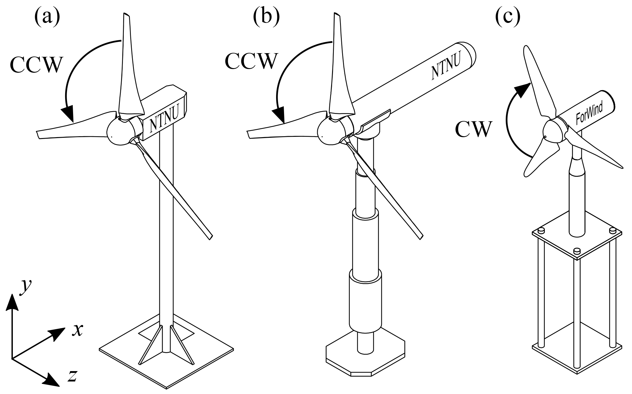
Figure 1Sketches of the model wind turbines with reference coordinate system, (a) NTNU turbine LARS1 rotating in counterclockwise direction (CCW), (b) NTNU turbine T2 rotating in counterclockwise direction (CCW), (c) ForWind turbine rotating in clockwise direction (CW).
The NTNU and ForWind rotors are based on two different airfoils. The NREL S826 airfoil, which is used from root to tip for the NTNU rotor, was originally designed for application in the tip region of full-scale wind turbines, a detailed description can be found in Somers (2005). It is designed for Reynolds numbers of Re, which is around 1 order of magnitude higher as the Reynolds number at the rotor tip in the presented experiments. Nevertheless, experimental data sets for airfoil performance at the lower Reynolds range around Re were measured at Denmark's Technical University (DTU; Sarlak et al., 2018) and NTNU (Bartl et al., 2018c). In Fig. 2 the airfoil polars from the DTU experiments at Re are compared to a standard set of lift and drag coefficients calculated for Re in XFoil, which was provided in the invitation document (Sætran et al., 2018). It can be seen that the drag coefficient CD is very different and the lift coefficient CL is significantly diverging from an angle of attack, α, of approximately 4∘ between the experimental and XFoil data. This difference is very distinct for high angles of attack that may occur close to stall.
The ForWind rotor is based on the SD7003 airfoil that is defined in detail in Selig et al. (1995). It is specifically designed for low Reynolds numbers and is thus well suited for wind tunnel experiments. In Selig et al. (1995) two experimental data sets for Re and Re are presented. They are in good agreement with XFoil data sets for Re and Re that were provided to the participants.
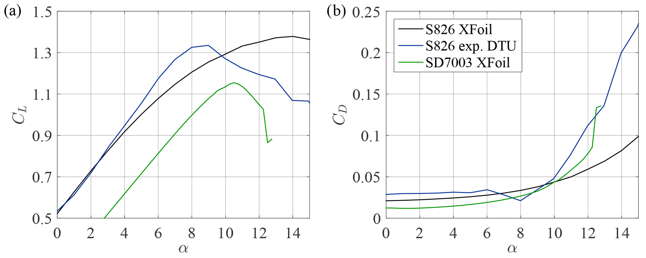
Figure 2(a) Lift coefficient and (b) drag coefficient for Re for NREL S826 from XFoil, NREL S826 from experiments DTU, and SD7003 from XFoil.
2.2 Wind tunnel and inflow condition
All the experimental data were measured in the closed-loop wind tunnel at the Department of Energy and Process Engineering at NTNU in Trondheim. The wind tunnel has a test section length of 11.5 m, a width of 2.7 m, and a height of 1.8 m. The reference coordinate system is pictured in Fig. 3 and a detailed description can be found in Sætran et al. (2018).
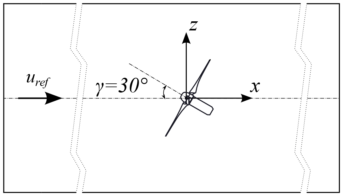
Figure 3Reference coordinate system in the wind tunnel and definition of positive yaw angle γ, top view.
For all test cases a nonuniform shear flow was generated by a grid at the inlet of the test section. The grid is built from wooden bars with a cross section of 0.047 m×0.047 m. In the horizontal direction the bars are evenly distributed with a distance of 0.24 m between the edges of the bars. In the vertical direction the mesh size increases with increasing height from a clearance of 0.016 m close to the floor to an opening of 0.30 m underneath the roof. The grid has a total solidity of about 34 % in the wind tunnel cross section. The shear profile can be described by the power law
The power law describes the wind speed as a function of the height y provided that the reference wind speed uref is known at a reference height yref. The strength of the shear is described by the power law coefficient α. The shear grid used in the experiments was designed to obtain an exponent of α=0.11.
As the velocities of the shear profile vary in height and are nonuniform over the rotor area, the reference wind speed uref is defined at the turbine hub height as shown in Fig. 4a. Furthermore, the velocity profile approximated by Eq. (1) matches well with the measured velocities, having a maximum deviation of ±1.0 %. Figure 4b shows the normalized vertical velocity component of the inflow for the NTNU turbine. It can be seen that the vertical flow component v is negative, which creates a slight downflow in the wind tunnel. The deviations in v from zero were not known at the time the blind test invitation was sent out, in which a zero velocity component for v was assumed. In order to take this into account, in the comparison, v at the inlet is subtracted from the vertical velocity component that is measured in the wake at the same y position.
The turbulence intensity (TI) of the inflow is shown in Fig. 4c. As expected, the turbulence decays with increasing downstream distance. At the position of the NTNU turbine the turbulence intensity is measured to be TI =10.0 % at hub height. The integral length scales Luu are calculated from hot-wire measurements of the streamwise velocity fluctuation u′ and the dissipation rate of the TKE E, by applying , where A≈1, taken from Krogstad and Davidson (2010). This results in Luu=0.097 m at the position of the NTNU turbine. The ForWind turbine was placed 5D (D=DLARS1) behind the shear grid and thus experienced a lower turbulence intensity of TI =5.2 %. The integral length scale, however, increased to Luu=0.167 m at this position. The third investigated streamwise position is 6D behind the NTNU turbine. At this position the turbulence has further decayed to TI =4.1 %. The corresponding integral length scale at this position is Luu=0.271 m.
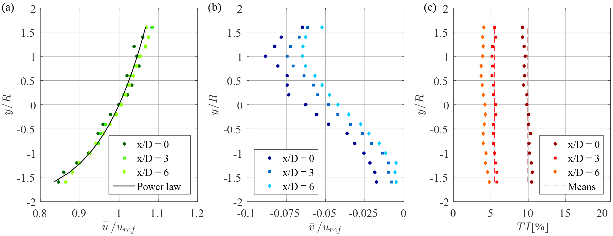
Figure 4Vertical flow profiles in the empty wind tunnel at different positions, in which refers to the position where the NTNU turbine is thereafter located: (a) normalized streamwise velocity u*, (b) normalized vertical velocity v*, and (c) turbulence intensity, TI (%). The radius R and diameter D refer to the NTNU turbine.
2.3 Test cases description
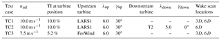
In this blind test experiment the modelers were asked to simulate three test cases. In test case 1 the flow 3D and 6D behind the yawed turbine LARS1 and its performance, thrust force, and yaw moment are investigated. The grid at the inlet is located −2D upstream of the turbine location at . The inflow velocity is adjusted to uref=10.0 m s−1 and the turbulence intensity is TI =10.0 % at the turbine's position. The turbine's hub height is in the center of the wind tunnel at hhub=0.89 m. LARS1 is yawed to and operated at its design tip speed ratio of λLARS1=6 throughout all measurements. In test case 2 a turbine operating in the wake of a yawed upstream turbine is investigated. Therefore, the setup of test case 1 is extended with the turbine T2 located D behind the upstream turbine LARS1. In contrast to LARS1, T2 is not yawed (γT2=0∘). As the downstream turbine is impinged by a partial wake of the upstream turbine, its optimum tip speed ratio is reduced to λT2=5, taking into account that the tip speed ratio is based on the constant reference velocity uref=10.0 m s−1 upstream of the two-turbine array. This test case investigates to what degree a partial wake impact can deflect the wake behind a non-yawed downstream turbine. This has recently been investigated in a LES study by Fleming et al. (2018). In test case 3, similar to test case 1, the flow 3D and 6D (D=DForWind) behind the ForWind turbine is investigated. The turbine is located at x=3D (D=DLARS1), which resulted in a lower turbulence intensity of TI =5.2 % at the turbine position. The hub height is set to hhub=0.89 m and the inflow velocity is reduced to uref=7.5 m s−1. Corresponding to test case 1 the turbine is yawed for γForWind=30∘ and is operated at its optimum tip speed ratio of λForWind=6. All setup parameters for test cases 1–3 are summarized in Table 1 and a detailed description can be found in Sætran et al. (2018).
Table 1Summary of the parameters that are varied for the three investigated test cases, up refers to the upstream and down to the downstream turbine position.
3.1 Measurement techniques
The u- and v-velocity components in the wake were measured using a two-component FiberFlow laser Doppler velocimetry (LDV) system from Dantec Dynamics. The LDV probe was placed inside the wind tunnel on a traverse system. For each measurement point, 5.0×10⁴ samples were recorded. The sampling frequency was adjusted by controlling the particles in the flow, ranging from 1500 to 2000 Hz, which resulted in an average sampling time of approximately 25–33 s.
The thrust force and yaw moments acting on the upstream and downstream turbine were measured separately using a Schencker six-component force balance, which was installed under the wind tunnel floor. The balance also served as a turning table allowing an exact adjustment of the yaw angle. For the rotor thrust only the load cell parallel to the flow was taken into account. The yaw moment was calculated from a moment equilibrium of three measured forces in the horizontal plane (referenced to the rotor center).
The aerodynamic power P of the NTNU rotors was measured using the test rig of turbine T2. This turbine is equipped with an optical RPM sensor (revolutions per minute) and a torque transducer in the hub. Thus, the torque T and the rotational speed ω of the turbine could be simultaneously measured so that .
3.2 Measurement uncertainties
The experimentally measured values feature several uncertainties. The statistical uncertainties in every sample of the mean velocity, power, thrust, and yaw moments are calculated based on a 95 % confidence level according to the procedure described in Wheeler and Ganji (2010). The uncertainty for the power measurements is calculated to be within ±3 %, while the force measurement uncertainty is slightly lower (±2 %). The exact values for all measured points are presented as error bars in the plots for the power coefficients CP, the thrust coefficients CT, and the yaw moments . The uncertainties for the mean streamwise velocities u in the wake are calculated to be smaller than ±1 %. The uncertainties for the vertical velocity component v are slightly higher due to the correction by the inlet component. In order to determine the inaccuracy in the TKE measurements, the method proposed by Benedict and Gould (1996) was applied. The uncertainties for a 95 % confidence level are found to be below ±2 % in the wake. It should be noted that the coarse measurement grid slightly influences the position of the TKE peaks.
3.3 Participants and computational methods
Siemens PLM Software from the United Kingdom (Siemens), the Department of Mechanical Engineering of the Politecnico di Milano in Italy (POLIMI), the Facultad de Ingeniería of the Universidad de la República in Uruguay (UdelaR), and KTH Mechanics Department from the Royal Institute of Technology in Sweden (KTH) participated in the blind test and submitted computational results. For clarity, only the abbreviations will be used in the following. A summary of the simulation methods and mesh properties is presented in Table 2.
Table 2Overview of simulation methods and parameters. Abbreviations: improved delayed detached eddy simulation (IDDES), large eddy simulation (LES), actuator line (ACL), and fully resolved (FR).
3.3.1 Siemens PLM Software (Siemens)
Siemens, who previously participated in blind test experiments as CD-adapco, used the finite volume code STAR-CCM+ v12.04 to mesh and solve all three test cases. Each simulation resolved the rotor, nacelle, and tower structure completely, and used the hybrid method improved delayed detached eddy simulation (IDDES), which resolves the energy-carrying eddies in the free stream and solves the boundary layer flow with RANS. The Spalart–Allmaras model was used for closure of the turbulence equations, and the fluid was considered incompressible. Convective fluxes used a MUSCL third-order scheme (monotonic upwind scheme for conservation laws), while time was discretized using a second-order implicit scheme. Each set of blades and hub was contained inside a cylindrical, rotating volume which was meshed with polyhedral cells, whereas the main domain used trimmed cells, resulting in a hexahedral dominant mesh in which a small proportion of cells was trimmed near the boundaries. Due to the rotation of the cylindrical volumes, the mesh was not conformal at the interface between the two regions, and flow quantities were interpolated from one volume to another. All wall surfaces, including the wind turbine bodies and the wind tunnel walls, were covered in several layers of prismatic cells to improve the resolution of boundary layers. The resulting y+ values were below 1 on the turbine bodies, and around 30 on the wind tunnel walls. The smallest cell size on the surface of the turbine bodies was 0.3 mm, typically found at the leading edge of the blades. The characteristic cell size in the rotating regions was 10 mm, which was also the cell size used in the wake of the rotors. The rest of the domain had a characteristic cell size of 20 mm. This resulted in meshes of 29×106, 35×106, and 17×106 cells for cases 1, 2, and 3 respectively.
While a rigorous mesh dependency study was not performed, the mesh sizes were based on previous experience and expected to perform well with an affordable amount of cells. All simulations were run with a time step of s, which was chosen to strike a balance between accuracy and computational cost. This value satisfies a number of criteria related to the rotation of the rotor regions; namely, that the rotors turn by less than 1∘ per time step, and that the mesh is moved by only half the cell size at the interfaces between rotating regions and the rest of the domain. Furthermore, it was verified a posteriori that the convective Courant number virtually never exceeded 0.3 in the wake of the turbines. Admittedly, given the small cell size used to mesh the blades, the time step causes the blades to move by several cell sizes each time step, and the Courant number to well exceed 1, particularly so near the blade tips. While this limits the ability to accurately resolve the flow at the blades, it was deemed sufficient to produce accurate wake results. The computational domain exactly matched the test section as described in the invitation document, i.e., 11.15 m long and 2.71 m wide and the wind tunnel walls were included as no-slip wall boundaries.
As inflow the given analytical mean velocity profile was used. Furthermore, the synthetic eddy method was used to superpose time-dependent eddies with the characteristic length scale of 10 mm, and a turbulence intensity TI =5 %. All cases were run for 1.6 s to establish the flow prior to sampling, and then mean values were sampled over a period of 2 to 3 s. An example using STAR-CCM+ can be found in Mendonça et al. (2012).
3.3.2 Politecnico di Milano (POLIMI)
POLIMI submitted a LES that was computed using the ALEVM code. It is an aerodynamic turbine simulation tool written in C++ and based on pisoFoam, which is an incompressible transient solver included in the OpenFOAM framework. The standard PISO (Pressure-Implicit with Splitting of Operators) solver was modified to include the effect of the turbine blades that are represented using the lifting line approach. The blade lines are discretized in segments based on the intersections with the numerical mesh grid, in which an actuation point acts on each segment. Each point of the actuator line (ACL) acts as an isolated blade section. More information about the ACL method can be found in Sørensen and Shen (2002). The wind velocity is numerically sampled for every blade point and used to compute the relative wind speed and the angle of attack. Thereafter, the aerodynamic forces are obtained through a look-up table, in which the blades' geometrical and aerodynamic properties are listed. Dynamic stall effects are not considered. In ALEVM the wind velocity is not sampled on a single point but averaged over a line, which is placed upstream of the blade point position with a distance proportional to the mesh cell dimension. The wind velocity is estimated using the mean of the velocity probed across the line. The main purpose of the relative wind speed estimation is in the angle of attack calculation. The wind velocity direction is then corrected to account for the local upwash due to the lifting line force. Based on the lifting line approach, the ALEVM code includes the turbine blade effect as an external momentum source term in the Navier–Stokes equations solved by the PISO algorithm.
ALEVM employs the well-known solution of the regularization kernel, smearing the line forces on the multiple cells following a Gaussian distribution and thus avoiding abrupt variation in the source term strength between adjacent cells. The turbulence in the wake region is modeled using a LES, adopting the Smagorinsky subgrid-scale model. For the time discretization scheme a first-order implicit approximation is used, while the divergence discretization scheme and the gradient discretization scheme are approximated by second order. The simulation is run for a time interval of 20 s, while a time step of s is used. This results in an angular rotation of about 2.4∘ per time step, which conversely means that 150 time steps make a full rotation. The resultant maximum Courant number of 0.21 is well below 1, indicating a sufficient temporal accuracy. The wind tunnel walls are included as no-slip boundaries, while the inlet turbulence grid is also geometrically modeled. The total cell count for the simulations is approximately 4.1×10⁶. Further details about the code can be found in Schito and Zasso (2014).
3.3.3 Universidad de la República (UdelaR)
UdelaR submitted another LES using their in-house developed caffa3d code. It is an open-source, finite volume code, with second-order accuracy in space and time, and parallelized with a message passing interface (MPI), in which the domain is divided into unstructured blocks of structured grids. Complex geometries are represented by a combination of body-fitted grids and the immersed boundary method over both Cartesian and body-fitted grid blocks. The code is F90 and currently runs on CPU, although a CUDA GPU version is currently being developed. The properties of the geometry and the flow are expressed as primitive variables in a Cartesian coordinate system, using a collocated arrangement. An ACL approach is used to discretize the turbine blades in the simulations. The aerodynamic forces on the blade elements are computed using the provided XFoil data, and dynamic stall effects are not considered. The forces, then, are projected onto the computational domain. In order to compute the additional source term, a Gaussian smearing function is used, taking into account one smearing factor for each direction: normal, tangential, and radial to the rotor plane. The domain, representing the wind tunnel (), is uniformly divided into grid cells in the streamwise, spanwise, and vertical directions, resulting in a total cell count of approximately 0.7×10⁶. A zero velocity gradient is imposed at the outlet, while a logarithmic law is used to compute the stress at the bottom wall and the symmetry boundary condition is used at the lateral and top boundaries. An implicit Crank–Nicolson time scheme is used with a time step of s, that corresponds to 0.16 of the rotor period (similar temporal resolution as used before, see for instance Guggeri et al., 2017). Both time step size and spatial resolution were defined based on previous simulations performed by UdelaR, particularly of Blind test 4. The scale-dependent dynamic Smagorinsky model is used to compute the subgrid-scale stress, using a local averaging scheme. The inflow condition is obtained from a precursor simulation with a similar numerical setup, but without model wind turbines and using a periodic boundary condition at the west and east boundaries with a constant pressure gradient as forcing term. The upstream model wind turbine is placed 2DLARS1 from the inlet boundary for test cases 1 and 2, while for test case 3 the model wind turbine is placed 5DLARS1 from the inlet boundary. UdelaR results are obtained after averaging the simulated data over 52.5 s for test cases 1 and 2 and 67.5 s for test case 3. More information about the application of caffa3d for wind energy simulations can be found in Guggeri et al. (2017), Mendina et al. (2014), and Usera et al. (2008).
3.3.4 Royal Institute of Technology (KTH)
A third LES was submitted by KTH. The spectral element code Nek5000 (Fischer et al., 2008), which was developed to solve the dimensionless, incompressible Navier–Stokes equations, was used. Each spectral element is discretized using Gauss–Lobatto–Legendre quadrature points on which the solution is expanded using Legendre polynomials. The LES applies a spatial filtering technique to the two highest modes to remove a part of the energy in the smallest scales and redistribute it to the lower modes thus stabilizing the numerical simulation. The domain is discretized using 7.98×10⁴ uniformly distributed spectral elements with ninth-order polynomials in each element, resulting in a total cell count of approximately 58×106. The numerical domain size corresponds to the dimensions of the wind tunnel. In the case of the NTNU turbine this mesh size corresponds to 45 grid points along each blade, when the blades are aligned with the mesh. The distance between the inlet and the first turbine is 4 rotor radii and the total length of the domain corresponds to 25 rotor radii. The dimensionless time step used to advance the simulation is , which corresponds to 0.1432 % of a rotor revolution and is chosen to satisfy the Courant–Friedrichs–Lewy condition. The wind turbine blade geometry is represented by body forces according to the ACL method with the lift and drag forces being computed using tabulated airfoil data. For the NTNU turbines the experimental airfoil data set from DTU (Sarlak et al., 2018) is used. It provides lift and drag coefficients over a range of Reynolds numbers. The ForWind turbine lift and drag forcing was computed using airfoil polars generated by XFoil that were provided in the invitation. Dynamic stall is not considered in the modeling approach. At the blade tips the Prandtl tip correction is applied. The forces computed at each actuator line are distributed using a three-dimensional Gaussian distribution. The Gaussian width is selected to be 2.5 times the average grid spacing. A mesh independency study of the non-yawed NTNU wind turbine established that using the aforementioned domain resolution combined with this Gaussian width provided a converged averaged wake development. The tower is also modeled using a body force approach. Both an oscillating lift component and a constant and oscillating drag component are included. The lift and drag coefficients for the mean drag and root-mean-squared lift and drag of a cylinder are taken from Summer and Fredsøe (2011). The line forces are then distributed using the three-dimensional Gaussian approximately in the volume occupied by the tower. This setup has been previously validated against experimental data from the NTNU turbine (Kleusberg et al., 2017). In the case of the ForWind turbine only the actual tower of the support structure is included. The turbulence at the inlet is modeled using sinusoidal modes with random phase shifts and they are scaled with a von Kármán energy spectrum. It is superimposed onto the desired uniform inflow condition. The turbulence is calibrated to give a turbulence intensity at hub height of approximately TI =10.0 % at the upstream turbine LARS1 and TI =4.8 % at the downstream turbine T2. At the outlet a zero-stress boundary condition is used while the symmetry boundary condition is imposed laterally to avoid resolving the wall boundary layer. More details about the computational setup can be found in Kleusberg et al. (2017). The velocity and TKE in the wake were temporally averaged over a dimensional time interval Δt= 4–5.3 s, which corresponds to over three flow-throughs of the numerical domain in the NTNU cases.
3.3.5 Wind turbine performance, forces, and moments
The modelers were asked to predict the power coefficients CP (Eq. 2), where P is the mechanical power of the turbine, ρ is the air density, and A the rotor swept area, as well as the thrust coefficients CT (Eq. 3), where T is the thrust force acting on the whole test rig, including rotor and tower, perpendicular to the rotor plane. Furthermore, the normalized yaw moments (Eq. 4) were required, where My is the yaw moment that is calculated by a moment equilibrium of the horizontal forces taking the distances of the load cells according to the center of the rotor plane into account. In test case 1 the power coefficient CP, LARS1, the thrust coefficient CT, LARS1, and the normalized yaw moment are compared. For the aligned turbine array in test case 2, the predictions for the upstream turbine are similar to test case 1. However, additional predictions of CP, T2, CT, T2, and for the downstream turbine were compared. Due to a high uncertainty in the power and thrust force measurements of the ForWind turbine, CP, ForWind, CT, ForWind, and are not compared in test case 3. The performance characteristics of the NTNU turbines are listed in Table 1.
3.3.6 Mean and turbulent wake flow
The modelers were asked to provide predictions of the velocities and TKE in full wake planes in the ranges and , respectively. The grid points are separated by 0.1D resulting in a grid consisting of 357 points, which is sketched in Fig. 5. The time-averaged streamwise and vertical velocities, u and v, for all points are normalized by uref so that and , respectively. The same procedure is applied for the TKE k, which is normalized to . The TKE in a three-dimensional flow is defined as
However, in the experiments only the two velocity components u and v were measured. Comparing u′ and v′ showed that the TKE is not perfectly isotropic. Therefore, additional measurements of the third velocity component w for one wake scan were performed to investigate whether the fluctuations v′ and w′ were in the same range. The results confirmed the assumption, allowing an approximation of the TKE as
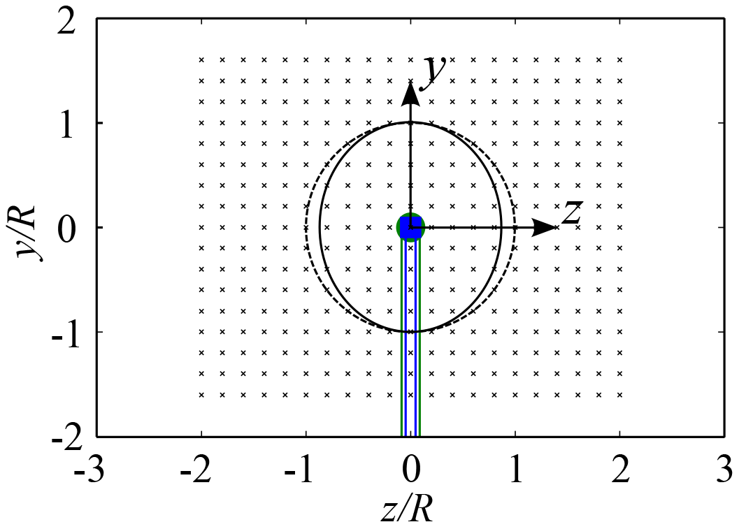
Figure 5Measurement grid in the wake consisting of 357 points, the blue tower and nacelle represents the NTNU turbine LARS1, the green tower and nacelle represents the ForWind turbine, the dashed line corresponds to the projection of the rotor diameter γ=0∘, the solid line corresponds to the projection of the rotor area γ=30∘, and the outline corresponds to the cross section of the wind tunnel with the NTNU turbine installed.
3.4 Comparative methods
Two-dimensional wake contours are difficult to compare quantitatively as they cannot be plotted in the same diagram. However, they provide valuable insight into the shape and position of the wake. Therefore, the wake shapes are in a first iteration compared qualitatively. To obtain quantitative measures of comparison, different methods to compute the wake position, the energy content in the wake, and the magnitudes of the wake parameters are applied. These are described below.
3.4.1 Available power method for wake deflection and energy content
In order to quantify the wake deflection, a method approximating the available power is used, which was previously described by Schottler et al. (2017). This method is deemed to be an appropriate approach to analyze the wake deflection of a yawed wind turbine as it takes the full wake scans into account. To find the wake center deflection, an imaginary rotor is laterally traversed in the wake while the wake center is defined as the position where the available power in the wake is the lowest. To get information about the energy content in the wake, the minimum of available power of the deflected wake is normalized by the available power found in the free stream of the experiment. With the resulting normalized minimum available power (), possible deviations in the location and magnitude of the energy content can be directly quantified.
3.4.2 Statistical methods for wake properties
From the statistical error measures proposed by Chang and Hanna (2004) the normalized mean square error (NMSE) and the correlation coefficient (r) are used to quantify the differences between simulations and experiments regarding u*, v*, and k*. For this purpose, all 357 points in the y–z plane of the CFD predictions are compared to the corresponding measurement points. Perfect predictions would result in NMSE =0.0 and r=1.0. They are calculated according to
where xe represents the experimentally measured values and xs are the simulated values. indicates the average of all 357 points of the full wake scans. The standard deviation of all points of the whole wake scan is given in σx. NMSE is a measure of mean relative scatter and thus reflects both systematic and random errors (Chang and Hanna, 2004); as the difference of every data point is squared, outliers are emphasized, which is not considered to be significant as no major outliers are expected. NMSE is used to analyze the predictions of u* and k*. The method is, however, not suited to evaluate the discrepancy of v*, because v* fluctuates around 0. Consequently the denominator of Eq. (7) also ranges around 0, which results in unrealistically high values for the NMSE. The correlation coefficient r represents a linear relationship between the measurements and predictions. It directly compares the measured and predicted values at a certain point. The predictions of all three investigated wake properties u*, v*, and k* are analyzed using the coefficient r.
4.1 Test case 1
4.1.1 Power, thrust, and yaw moment
The results of CP, LARS1, CT, LARS1, and for test case 1, in which the turbine is operated at , are depicted in Fig. 6. For λ=6 the differences between the experimental and numerical results are summarized in Table 3. Comparing the values of CP, LARS1 in Fig. 6a it can be seen that the simulation results deviate from the measurements by up to 19 %. This is a larger scatter compared to the previous blind tests, e.g., Bartl and Sætran (2017). However, it should be kept in mind that the complexity is increased by the yawed turbine operation. Siemens, who fully resolved the rotor, overpredict CP, LARS1 by 14.2 %, which is almost in the same range as UdelaR and POLIMI who used ACL with the provided polars from XFoil and showed deviations of 18.5 % and 16.8 %, respectively. KTH also applied an ACL model, but used the experimentally generated data set of airfoil polars from DTU (Sarmast and Mikkelsen, 2012). Using these data results in a good agreement with the experimental data with only a slight underprediction of 2.3 %.
The blade element momentum (BEM) tool Ashes (Thomassen et al., 2012) was used to analyze the blade loads. The calculations showed that the angle of attack for the yawed turbine, which is defined similar to two-dimensional conditions as the angle between relative wind direction and the blade chord, is fluctuating approximately 2.0∘ during one rotation in the outer third of the blade, causing very high angles of attack. Note that the definition of the angle of attack is herein based on a simplified two-dimensional analysis, which omits the lateral component in the relative velocity during yaw. From Fig. 2, it can be seen that the lift and drag coefficients from the DTU experiments and XFoil are very different for such high angles of attack. The experimental polars from DTU seem to be more accurate as the polars predicted with XFoil for such high angles of attack, which explains the better predictions of CP by the simulations using the experimental polars.
The thrust coefficients CT, LARS1 for the single yawed turbine LARS1 are presented in Fig. 6b and only show a small scatter of up to 7.0 % around the experimental results and thus are almost all within the measurement uncertainty. Consequently, for CT predictions the experimental polars do not yield better results with respect to the polars generated by XFoil. The yaw moment is presented in Fig. 6c, over a range of yaw angles from ∘ to ∘. All simulations underestimate the experimental value of while the deviations ranging from about 30 % to 80 % are rather large. Nevertheless it should be kept in mind that the values of are very small and thus small deviations result in large differences in percentage.
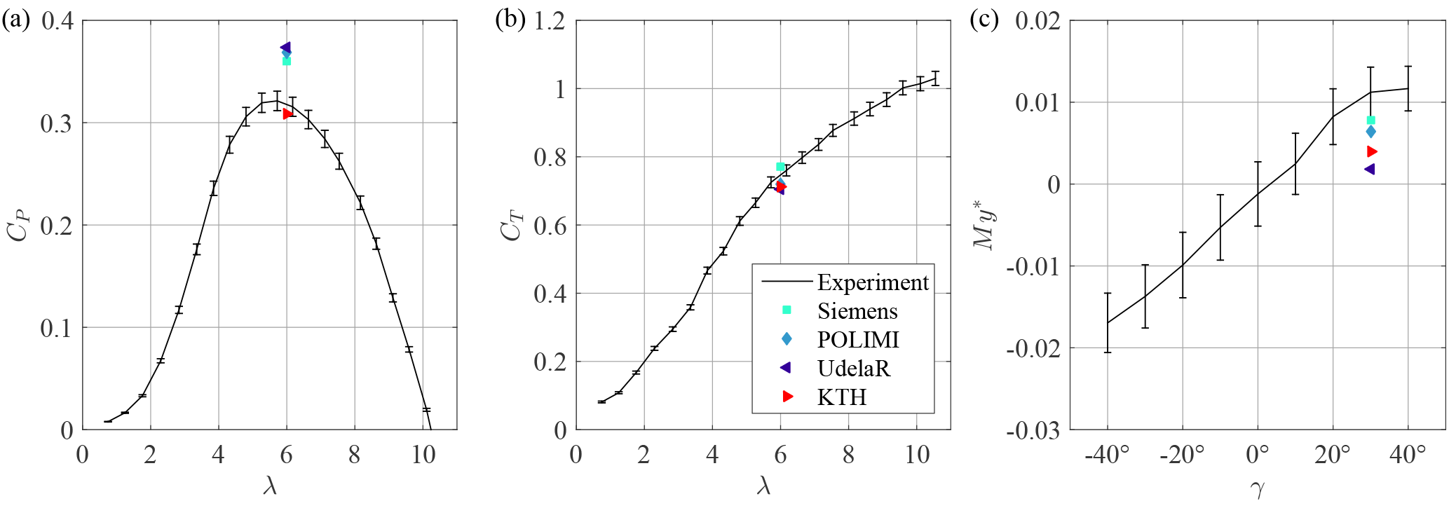
Figure 6Power coefficient CP, LARS1 (a) and thrust coefficient CT, LARS1 (b) for the upstream turbine LARS1 operated at γLARS1=30∘ and normalized yaw moment (c) for the upstream turbine LARS1 operated at λLARS1=6 for ∘ to +40∘.
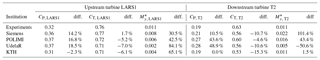
Table 3Numerical values of power coefficient CP, thrust coefficient CT, and normalized yaw moment and deviations of predictions to measurements in percent for test cases 1 and 2.
4.1.2 Wake characteristics
Figure 7 shows a comparison of the predictions of the time-averaged streamwise velocity u* at x=3D, with line profiles at hub height added to the full wake contours. The wake contours as presented in Fig. 7b show a slightly curled wake shape. The curled wake shape was shown to develop from a counter-rotating vortex pair, as discussed in detail by Schottler et al. (2018a) and Bartl et al. (2018b) for the same experimental data set. Similar flow physics behind a yawed turbine were observed in simulations by a full-scale turbine by Howland et al. (2016) and Vollmer et al. (2016). The wake shape is generally well predicted by three of the simulations. Only the wake predicted by UdelaR has a rather oval shape. As expected, the wake is not only curled but also clearly deflected in the negative z direction. This is very well predicted by all the simulations. POLIMI and KTH match the deflection, whereas UdelaR and Siemens slightly underestimate it. This is not consistent with the predictions of CT in which all institutions except Siemens estimate a lower CT. The tower shadow is also clearly visible in all simulations. By fully resolving the rotor and turbine geometry Siemens matches the experimental results almost perfectly. UdelaR and KTH, who both modeled tower and nacelle with a line of drag forces, simulate a fairly accurate tower shadow. Even though POLIMI did not model nacelle and tower, their results show a strong velocity deficit in the area where the tower shadow is expected. This effect is considered to be caused by the flow velocities modeled near the wind tunnel floor, whose influence is pronounced in all simulations by POLIMI. In the free stream, the shear flow can be clearly seen in the experimental results. Siemens, UdelaR, and KTH apply a user-defined shear function at the inlet and thus predict a smooth shear profile, while POLIMI, who fully resolved the turbulence grid at the inlet, simulate a shear profile with a too strong shear and very low velocities close to the floor. Figure 7a shows that POLIMI generally predicts lower velocities in the free stream, as the normalized velocity u* at hub height does not reach 1.0 in the free stream. Nevertheless, the velocities behind the rotor are represented very well, while a poor NMSEu of 0.017 and a ru of 0.878 show the discrepancy in the free stream to the measurements. All in all, it can be seen that u* is predicted well by all simulations. Siemens' results for this test case are almost perfectly in accordance with the experiments, which results in a very low NMSEu of 0.002 and a large ru of 0.964. Good statistical performance values are also achieved by KTH (NMSEu=0.002, ru=0.957), even though the velocity deficit in the wake center is slightly underestimated. An even clearer underprediction of the velocity deficit in the wake center can be observed for the UdelaR simulations, which result in a NMSEu of 0.005 and a ru of 0.914. These observations are confirmed by comparing the available power levels in the wake (Table 4). In the case of Siemens' accurate simulations of u*, only deviates by −2.7 % from the experiments. UdelaR underestimates the velocity deficit in the center significantly, resulting in an overprediction of by 42.7 %. KTH also overestimates by 15.6 %, which confirms the higher velocities observed in the wake center. The available power method shows a good agreement of POLIMI's simulations with the experiments, deviating only 11.2 %. This is because the method takes only the area in the wake center into account and thus is not affected by the deviating velocity levels in the free stream.

Figure 7(a) Line plot at hub height and (b–f) contour plots for normalized streamwise mean velocity u* in the wake 3D behind turbine LARS1, from (b) experiments, (c) Siemens, (d) POLIMI, (e) UdelaR, and (f) KTH. The white lines represent the turbine rotor, nacelle, and tower; solid lines γ=30∘; dashed lines γ=0∘.
Next, Fig. 8 shows the normalized vertical flow component v*. In general the velocity contours are dominated by two major flow patterns: a larger-scale dipole, characterized by flow from the ceiling to the center () and from the bottom to the center (); and a smaller dipole at the rotor edge at , where v* is positive outside the rotor swept area and negative in the rotor swept area featuring strong gradients between the peaks. These structures are generally predicted fairly well. Siemens, POLIMI and KTH match the flow pattern very accurately, which is confirmed by the line plots at hub height (Fig. 8a). High values of the correlation coefficient rv for these three simulations range from 0.819 to 0.866 and confirm the observations. The simulation by UdelaR (Fig. 8e) does not show very strong gradients and thus does not capture the detailed flow patterns. This is assumed to be due to a rather coarse mesh resolution for this simulation and can be seen in the low rv value of 0.383. Nevertheless, the general shape showing the large-scale structures on the right is captured well.
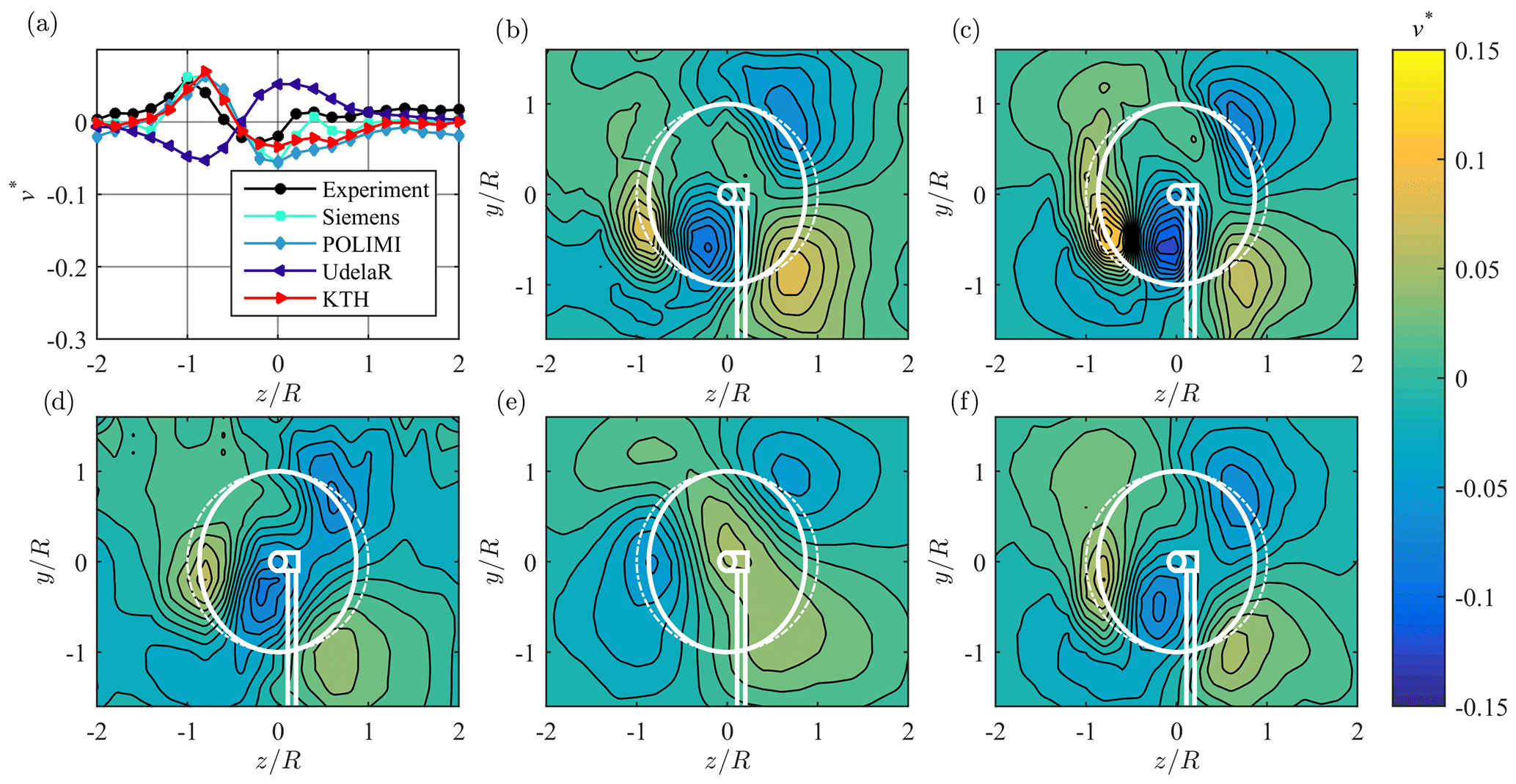
Figure 8(a) Line plot at hub height and (b–f) contour plots for normalized vertical mean velocity v* in the wake 3D behind turbine LARS1, from (b) experiments, (c) Siemens, (d) POLIMI, (e) UdelaR, and (f) KTH. The white lines represent the turbine rotor, nacelle, and tower; solid lines γ=30∘; dashed lines γ=0∘.
The normalized TKE k* is presented in Fig. 9. The contours show a clear ring of turbulence located around the rotor area. Similar to the shape of u* the ring is slightly compressed at the right side. Figure 9a shows that all simulations predict the position and magnitude of the turbulence peaks very well. Larger differences between measurement and simulations can be found outside of the ring. Here, Siemens predicts a very low TKE close to in the free stream and in the wake center. This underprediction of k* is assumed to be due to the rather large cell size in the free stream that is too coarse to sustain the free stream turbulence. It results in a rather large NMSEk of 0.663, whereas rk with 0.873 suggests a good correlation of the shapes. POLIMI's prediction of k* shows a higher background turbulence, especially below the rotor area in the positive z direction. These discrepancies result in poor statistical performance values of NMSEk=0.332 and rk=0.583. UdelaR's results show a clear shear profile of k* with increasing turbulence towards the wind tunnel floor. This is quite different from the experimental results; therefore, the values of NMSEk=1.045 and rk=0.333 are observed to be far off. The simulations of KTH are in very good agreement with the experiments which is confirmed by a low NMSEk of 0.085 and high rk of 0.924.
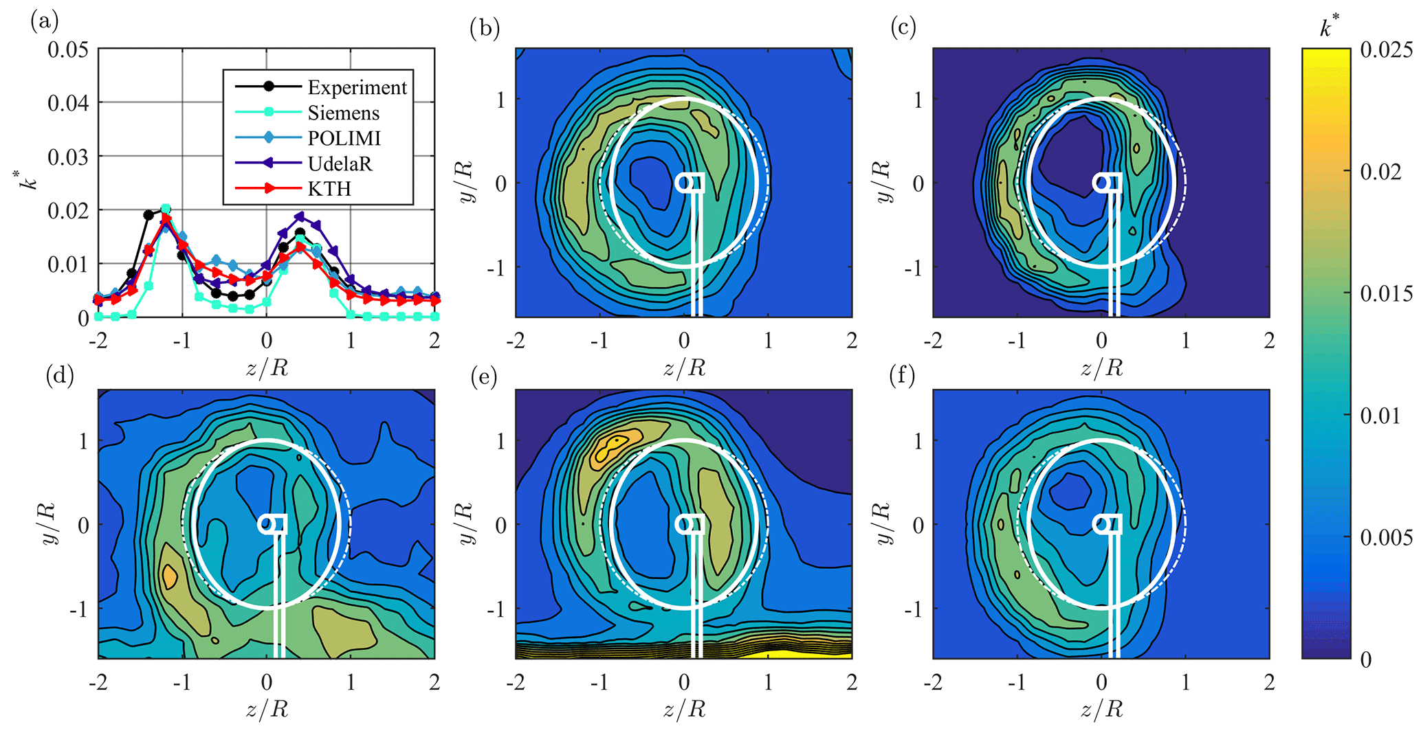
Figure 9(a) Line plot at hub height and (b–f) contour plots for normalized turbulent kinetic energy (TKE) k* in the wake 3D behind turbine LARS1, from (b) experiments, (c) Siemens, (d) POLIMI, (e) UdelaR, and (f) KTH. The white lines represent the turbine rotor, nacelle, and tower; solid lines γ=30∘; dashed lines γ=0∘.
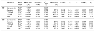
The comparisons of u*, v*, and k* 6D behind LARS1 show similar trends as already observed at a distance of 3D. Therefore, the results at 6D are not shown. The comparison parameters summarized in Table 4 confirm these observations. A major difference to the wake at 3D is a more distinct curled wake shape, which is generally well predicted by all simulations. The wake is further deflected, while the skew angle is lower compared to the observations at x=3D (Table 4). This is expected to be due to the large blockage ratio of the NTNU turbine and the interference of the wake with the wind tunnel walls. The experimental results of the wake at x=6D are also documented by Bartl et al. (2018b).
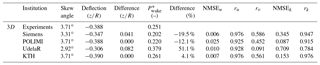
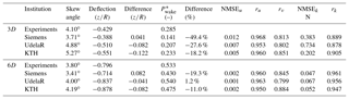
Table 4Comparison parameters: skew angle (ξ), wake deflection (δ) and available power in the wake () and their differences to the measurements. Statistical performance measures: NMSE and r for u*, v* and k* at 3D and 6D behind upstream turbine LARS1.
4.2 Test case 2
4.2.1 Power, thrust, and yaw moment
In test case 2 an aligned turbine array with both NTNU turbines LARS1 and T2 is investigated. The upstream turbine LARS1 is operated at γLARS1=30∘ and λLARS1=6.0. Consequently, CP, LARS1, CT, LARS1, and are identical to test case 1 (Fig. 6, Table 3) and are therefore not further discussed here. The downstream turbine T2 is operated at γT2=0∘ and λT2=5.0. The tip speed ratio λT2=5.0 is computed using the far-upstream reference velocity uref=10.04 m s−1. T2 is located 3D behind the yawed upstream turbine, meaning that the wake flow of test case 1 represents the inflow for T2. Detailed results of power, thrust, and yaw moments for the upstream and downstream turbine operated at different yaw angles, separation distances, and inflow conditions are presented by Bartl et al. (2018a). Previous blind tests discussed the higher spread in prediction results of a downstream turbine's performance. This is confirmed by comparing CP, T2, CT, T2, and of T2, which show a significantly larger spread of performance than for test case 1 (Fig. 10, Table 3). The simulation results of the downstream turbine's power coefficient CP, T2 (Fig. 10a) deviate between 0 % and 48.9 % from the experimental results. KTH matches the experimental value exactly and thus confirms the good forecast from test case 1. Siemens predicts the available power in the wake fairly accurately and thus overestimates CP, T2 by only 10.5 %. POLIMI and UdelaR over estimate CP, T2 significantly by 43.6 % and 48.9 %, respectively. This trend could already be seen for the upstream turbine power coefficient CP, LARS1 and is enhanced by overpredicting the available power in the wake for UdelaR. POLIMI prognosticates less available power in the wake. The simulation results of the downstream turbine thrust coefficient CT, T2 (Fig. 10b) show smaller deviations than those for CP, T2. Nevertheless, they are slightly larger than those of CT, LARS1 in test case 1. All simulations underestimate CT, T2 while KTH's result shows the largest deviation of −15.3 % compared to their accurate prediction of CP, T2. Siemens and UdelaR show a similar thrust that deviates from the experimental value by −10.7 % and −10.6 %, respectively. POLIMI underpredicts CT, T2 by 4.6 %. A larger spread is again observed for the simulations of (Fig. 10c) as the values for are very small and consequently more difficult to predict. Siemens and POLIMI are observed to overestimate by 101.4 % and 43.3 %, respectively. UdelaR underpredicts for 50.6 % while KTH matches the experimental results very accurately with only 1.5 % difference.
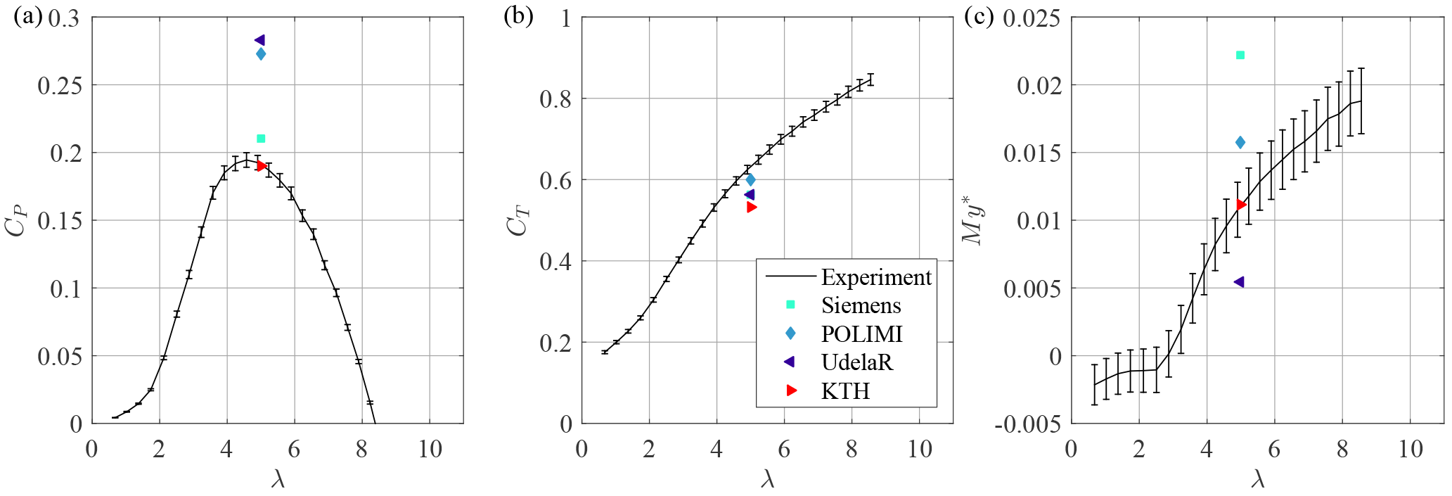
Figure 10Power coefficient CP, T2 (a), thrust coefficient CT, T2 (b) and normalized yaw moment (c) for the T2 downstream turbine operated in the wake of LARS1 at γT2=0∘ for λT2=1 to 12.
4.2.2 Wake characteristics
This section discusses the wake characteristics 3D behind the two-turbine array. The wake is clearly deflected in the negative z direction. However, the deflection is not as big as 6D behind the single yawed turbine, but rather in the same range as 3D behind the single yawed turbine. These results compare well with a recent LES study by Fleming et al. (2018), who simulated a similar wake deflection behind a non-yawed downstream turbine exposed to a partial wake inflow. This suggests that a further wake deflection is restricted by the non-yawed downstream turbine and maintained at approximately the same level at which it hits the downstream turbine. Moreover, the wake shape does not show a curled shape, instead being rather oval (Fig. 11). The tower shadow, which is mainly formed by the T2 downstream turbine tower, is more centered than in test case 1 and is well predicted in all simulations. The shear profile in the free stream is well captured by all simulations. However, all predictions show a slightly lower velocity level than in the experiment. POLIMI's simulations indicate a rather strong velocity gradient again, with very low velocities close to the wind tunnel floor. However, the gradient is better established than in test case 1 as it develops further downstream. The line plot in Fig. 11a confirms that all the simulations underestimate the additional speed-up around the downstream turbine rotor. Siemens overpredicts the velocity deficit in the wake center which is confirmed by the available power that is 19.5 % lower as the one resulting from the experiments. Considering the whole wake scan, the statistical performance parameters NMSEu=0.006 and ru=0.976, on the other hand suggest better agreement. POLIMI predicts the velocities in the wake very accurately and estimates only 12.1 % lower than in the experiments. The statistical measures, however, do not confirm the good match of the energy level, resulting in a NMSEu of 0.025 and a ru of 0.925. The too low velocities in the free stream, which are not considered in , are deemed to impair the correlation coefficients here. The available power of UdelaR exceeds that of the experiments clearly by 51.1 %, which is mainly due to an underprediction of the velocity deficit in the wake center. Nevertheless, the statistical parameters that take the whole measurement grid into account, suggest a good agreement with NMSEu=0.010 and ru=0.928 as the lower velocities in the free stream counterbalance the higher velocities in the wake center. The velocity levels in the wake center are overpredicted by KTH; however, the available power is in good agreement with the experiments and only deviates 4.1 %. This is confirmed by good statistical values of NMSEu=0.007 and ru=0.976. The wake deflection is predicted well by all simulations. POLIMI and KTH match it accurately, whereas Siemens underpredicts it by and UdelaR by .
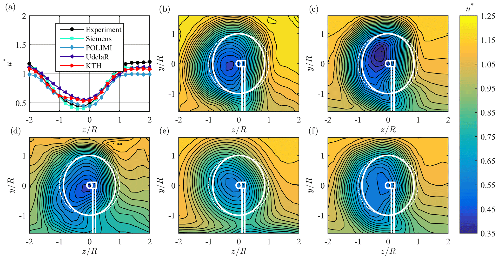
Figure 11(a) Line plot at hub height and (b–f) contour plots for normalized streamwise mean velocity u* in the wake 3D behind downstream turbine T2, from (b) experiments, (c) Siemens, (d) POLIMI, (e) UdelaR, and (f) KTH. The white lines represent the turbine rotor, nacelle, and tower; solid lines γ=30∘; dashed lines γ=0∘.
The contours of the vertical velocity component v* behind the turbine array show a similar flow pattern as the one behind the single yawed turbine (Fig. 12). Nevertheless, the magnitudes of v* are smaller compared to test case 1. The flow pattern is described fairly accurately by all simulations. However, Siemens, POLIMI, and KTH have average correlation values rv ranging from 0.452 to 0.586. The predictions by UdelaR are again rather coarse and thus reveal less details, which results in an even lower linear correlation coefficient of only rv=0.091.
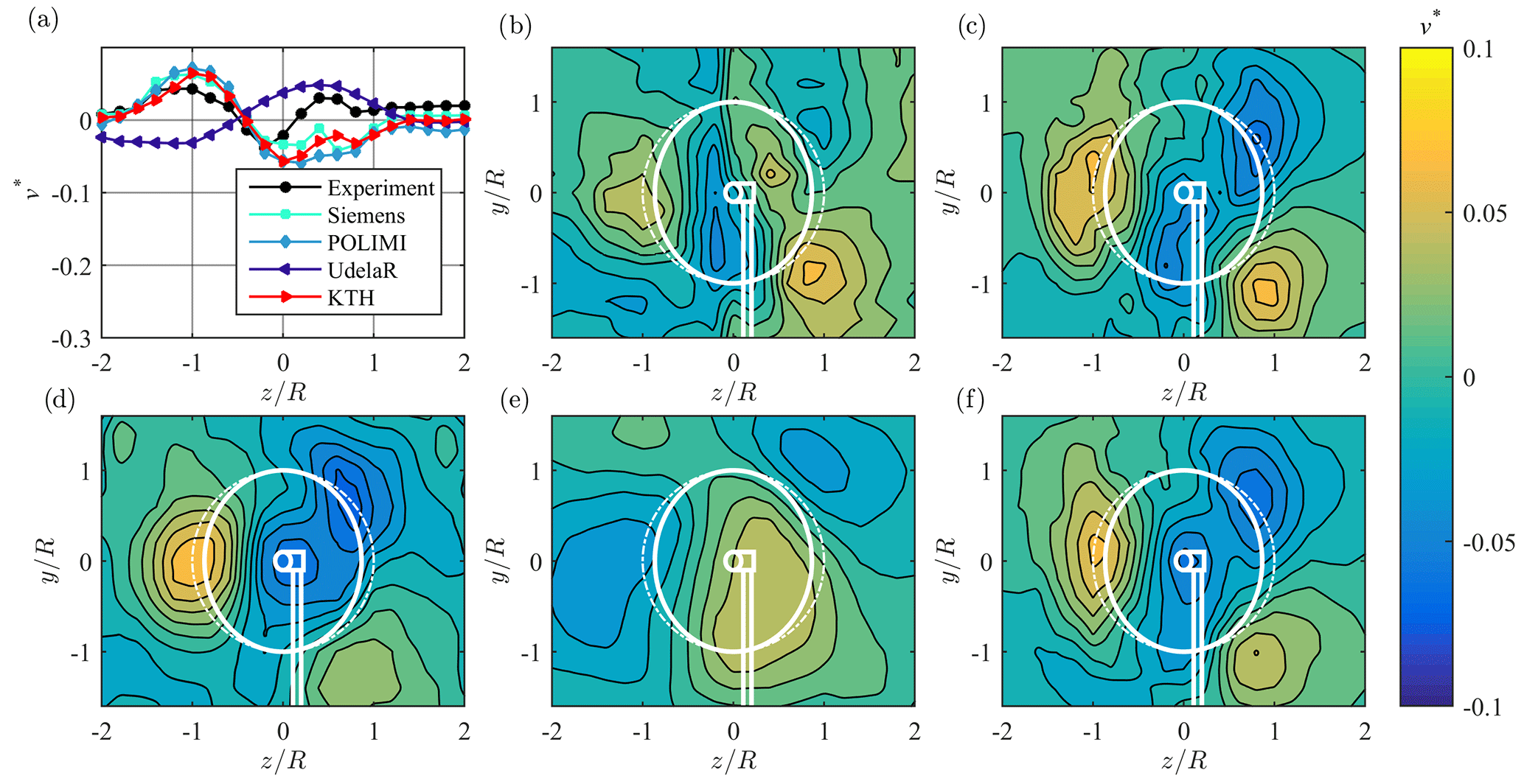
Figure 12(a) Line plot at hub height and (b–f) contour plots for normalized vertical mean velocity v* in the wake D behind downstream turbine T2, from (b) experiments, (c) Siemens, (d) POLIMI, (e) UdelaR, and (f) KTH. The white lines represent the turbine rotor, nacelle, and tower; solid lines γ=30∘; dashed lines γ=0∘.
The TKE k* in the wake behind the turbine array as shown in Fig. 13 is characterized by a ring of higher TKE that is deflected in the same way as u* and thus is similar to test case 1. Compared to the single turbine wake, the ring of high TKE is observed to be broader and flattened out (Fig. 13a). The peak locations are prognosticated very well by all simulations. However, Siemens and KTH underpredict the levels of k*, while UdelaR overpredicts the turbulence in the ring, especially on the right hand side of the wake. POLIMI seems to match the turbulence in the ring fairly accurately which results in a low NMSEk of 0.087 and rk of 0.915. Good rk values are also obtained by Siemens and KTH with rk=0.947 and rk=0.976, respectively. However, their NMSEk values of NMSEk=0.345 and NMSEk=0.153, respectively, suggest some deviations. The overprediction of TKE by UdelaR results in slightly poorer statistical performance values of NMSEk=0.709 and rk=0.784.
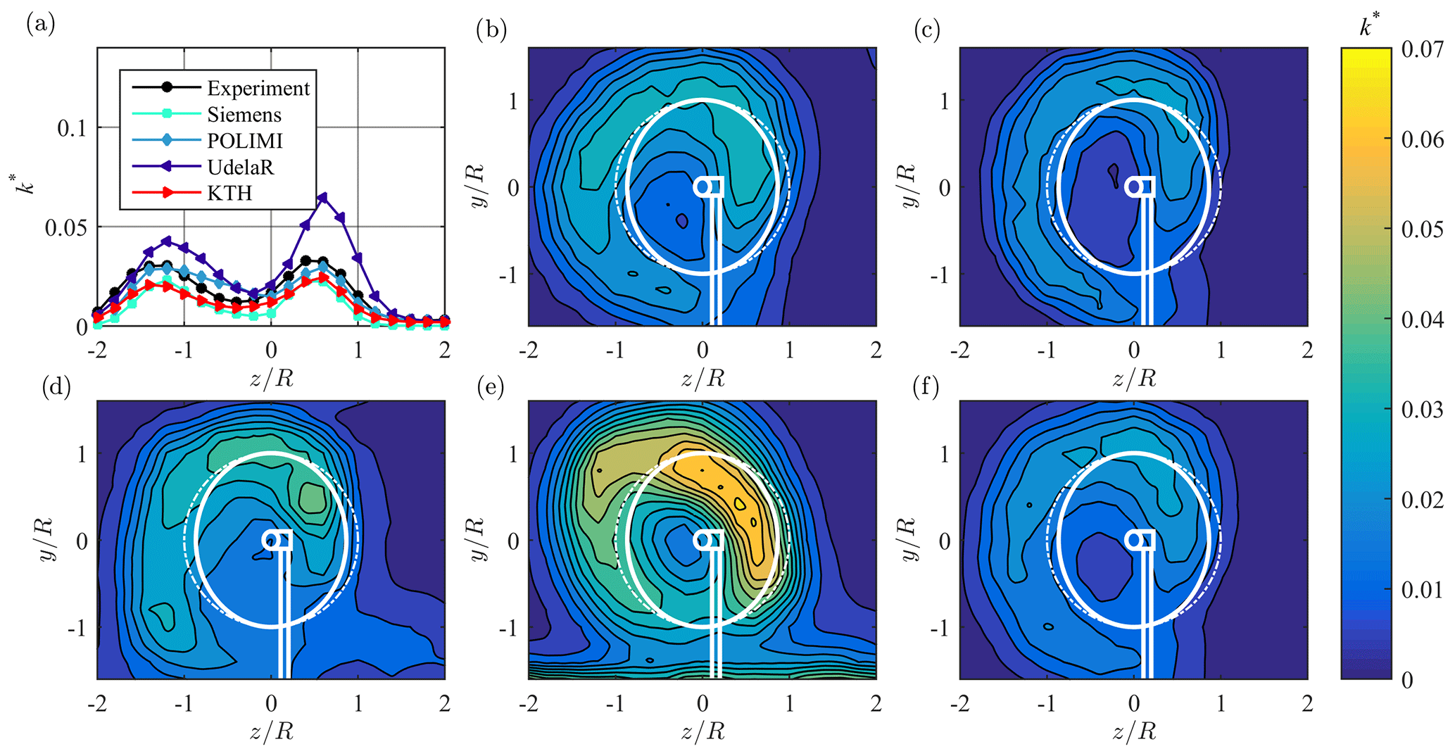
Figure 13(a) Line plot at hub height and (b–f) contour plots for normalized turbulent kinetic energy (TKE) k* in the wake 3D behind downstream turbine T2, from (b) experiments, (c) Siemens, (d) POLIMI, (e) UdelaR, and (f) KTH. The white lines represent the turbine rotor, nacelle, and tower; solid lines γ=30∘; dashed lines γ=0∘.
Table 5Comparison parameters: skew angle (ξ), wake deflection (δ) and available power in the wake (), and their differences to the measurements. Statistical performance measures are NMSE and r for u*, v*, and k* at 3D behind downstream turbine T2.
4.3 Test case 3
4.3.1 Wake characteristics
In the third test case the wake behind the yawed ForWind turbine is investigated. It was simulated by three of the modelers, while POLIMI did not submit predictions for this test case. The contours of the streamwise velocity 3D (D=DForWind) behind the ForWind turbine are presented in Fig. 14b–e. They show a more distinct curled wake shape than that observed for the NTNU turbine. In contrast to the NTNU turbine, the ForWind turbine rotates in a clockwise direction when observed from upstream. A counterclockwise wake rotation deflects the wake center to the lower half behind the rotor as described in detail by Schottler et al. (2018a). Furthermore, it can be seen that due to the smaller rotor diameter there is less blockage which reduces the speedup around the rotor significantly (Fig. 14a). Thus, a smooth shear profile is observed in the free stream. The velocity deficit as well as the curled wake shape are predicted very well by all simulations with only UdelaR's simulations showing a less distinct curl. The position of the largest velocity deficit is consistent for all simulations. Nevertheless, most participants overestimate the magnitude of the velocity deficit. Siemens has the largest deviations from the experiments, which results in an available power that is 49.4 % lower compared to the measurements. However, when not only taking the imaginary rotor area into account but also considering the whole wake scan, the statistical performance values NMSEu=0.012 and ru=0.968 indicate a good agreement. UdelaR predicts velocities that result in only 27.6 % less available power for a potential downstream turbine, but NMSEu=0.007 and ru=0.953 are in the same range as the Siemens predictions and indicate a good match of the whole wake scan. The KTH simulation matches the experimental results best and shows the smallest deviation of available power and with NMSEu=0.005 and ru=0.960 their statistical performance values confirm the good agreement. The wake of the ForWind turbine is slightly more deflected than 3D behind the NTNU turbine (Table 6). Siemens again underpredicts the deflection, whereas UdelaR and especially KTH predict a stronger deflection of the wake than observed in the experiments.
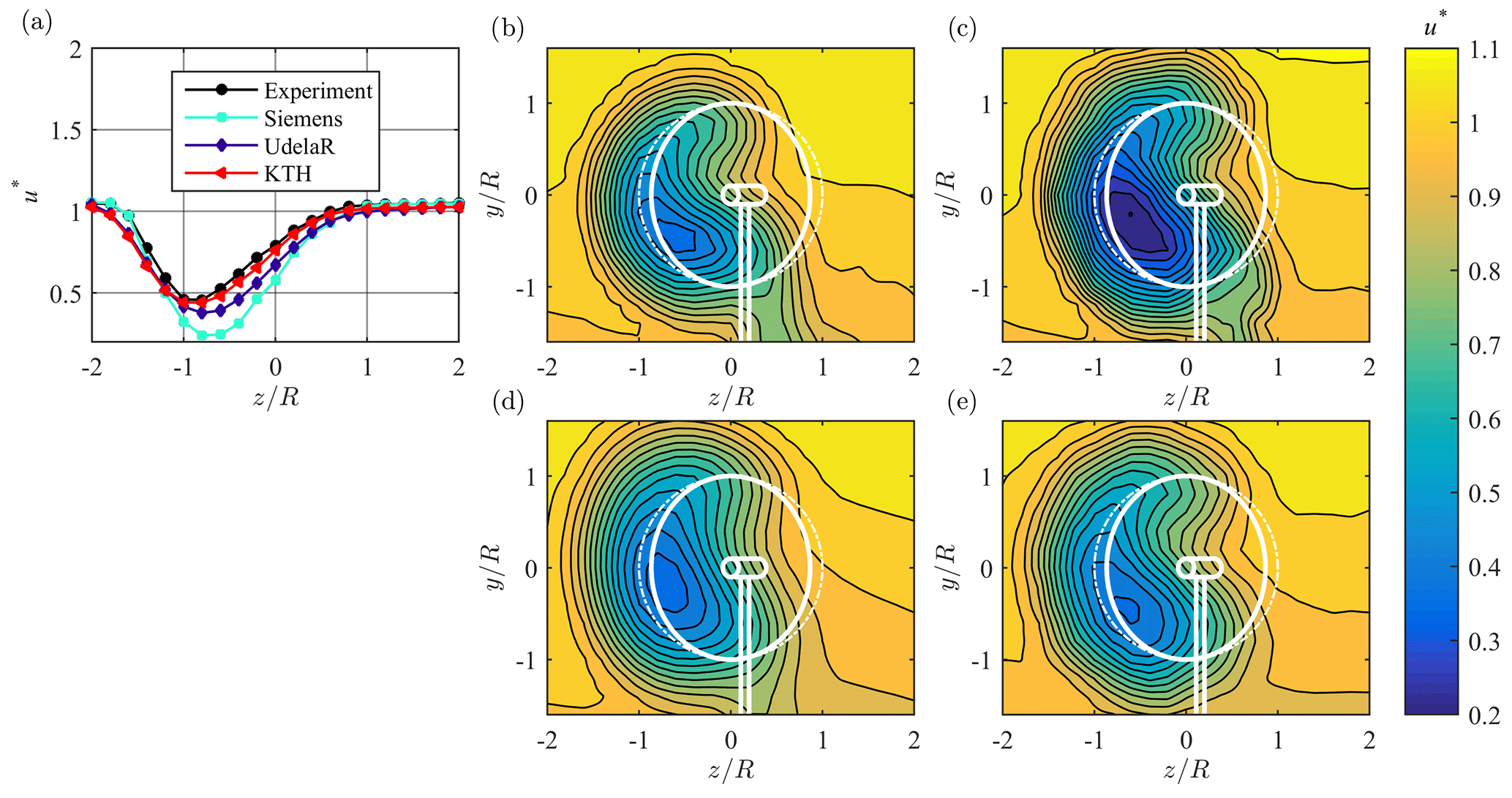
Figure 14(a) Line plot at hub height and (b–e) contour plots for normalized streamwise mean velocity u* in the wake 3D behind ForWind turbine, from (b) experiments, (c) Siemens, (d) UdelaR, and (e) KTH. The white lines represent the turbine rotor, nacelle, and tower; solid lines γ=30∘; dashed lines γ=0∘.
The contours of the normalized vertical velocity v* (Fig. 15b–e) are similar to those observed 3D behind LARS1. The flow field is dominated by the same major flow patterns as already observed in test case 1. The major difference is that the peaks in the positive z direction are more centered and that the dipole at the left rotor edge is not as distinct. All simulations of v* match the experiment fairly accurately, which results in similar rv values ranging from 0.802 to 0.851. Siemens, however, predicts slightly higher positive peaks, but the distribution of v* is captured very well. The same applies for KTH and UdelaR, who again predict smoother gradients due to a coarse mesh resolution.
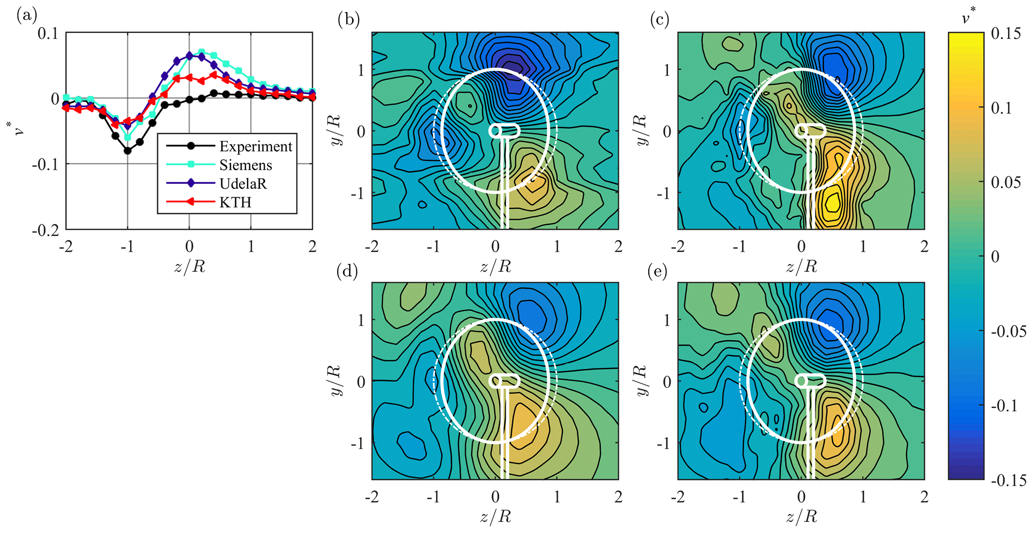
Figure 15(a) Line plot at hub height and (b–e) contour plots for normalized vertical mean velocity v* in the wake 3D behind ForWind turbine, from (b) experiments, (c) Siemens, (d) UdelaR, and (e) KTH. The white lines represent the turbine rotor, nacelle, and tower; solid lines γ=30∘; dashed lines γ=0∘.
The TKE contours presented in Fig. 16b–e also indicate a clear curled shape. The k* values behind the ForWind turbine are observed to result in a significantly wider peak in the positive z direction (Fig. 16a) than observed behind LARS1. In contrast to the previous test cases, k* is distributed more smoothly over the wake which results in higher turbulence levels in the wake center. The shape of the TKE contours is accurately represented by all simulations. Siemens and UdelaR, however, over estimate the peak magnitudes significantly, while Siemens predicts the peak location in the upper half accurately. UdelaR's simulation is observed to result in higher TKE values in the whole ring. The simulations of KTH are in closest agreement with the experiments. The linear correlation coefficients are in the same range (rk=0.878–0.905) for all three predictions. Larger deviations can be observed in NMSEk that range from 0.202 to 0.734.
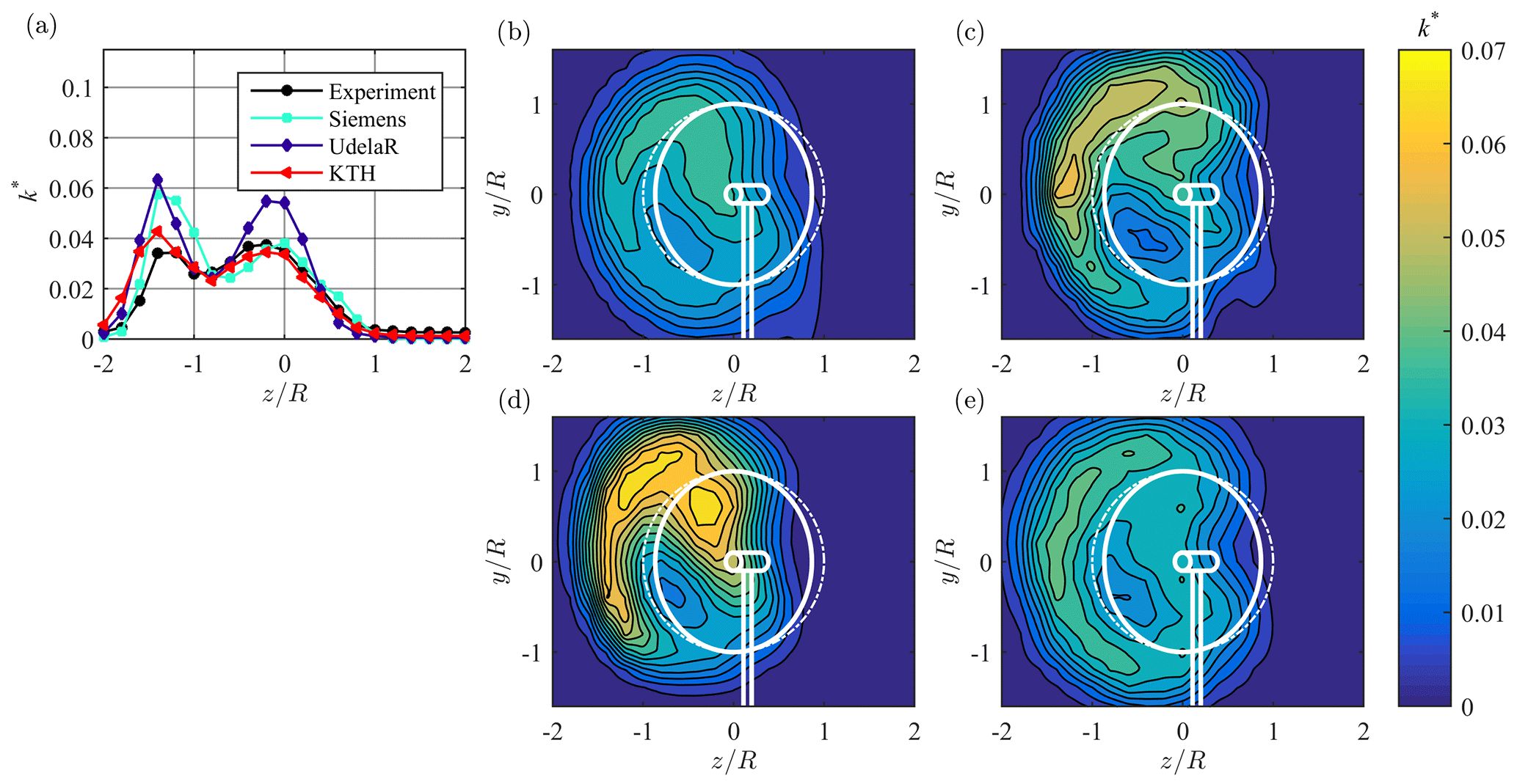
Figure 16(a) Line plot at hub height and (b–e) contour plots for normalized turbulent kinetic energy (TKE) k* in the wake 3D behind ForWind turbine, from (b) experiments, (c) Siemens, (d) UdelaR, and (e) KTH. The white lines represent the turbine rotor, nacelle, and tower; solid lines γ=30∘; dashed lines γ=0∘.
Table 6Comparison parameters: skew angle (ξ), wake deflection (δ), and available power in the wake (), and their differences to the measurements. Statistical performance measures are NMSE and r for u*, v*, and k* at 3D and 6D behind upstream ForWind turbine.
The comparison of the wake characteristics 6D behind the yawed ForWind turbine results in conclusions similar to those at 3D. Therefore, the figures comparing u*, v*, and k* 6D behind the ForWind turbine are not shown here, but the comparison parameters and statistical performance measures are listed in Table 6. The streamwise velocity u* and the vertical velocity v* are generally predicted accurately, which is represented by better comparison parameters and statistical performance values at 6D than at 3D for all simulations.
The results of four different computational contributions were compared to experimental wind tunnel results in this blind test experiment. The modelers submitted predictions for the performance of two single yawed turbine models and an aligned turbine array where only the upstream turbine is yawed. Furthermore, they predicted the mean and turbulent wake flow behind two different model turbines and the turbine array.
The power of a single yawed turbine CP, LARS1 was predicted with a scatter of ±19 %, which was slightly bigger than in the two previous blind test experiments. A bigger scatter of ±49 % is observed in the predictions of the power coefficient CP, T2 for a downstream turbine operating in partial wake conditions of the yawed upstream turbine. This variation is significantly larger than the scatter for an aligned downstream turbine operated in a full wake in the Blind test 4 workshop (Bartl and Sætran, 2017), in which a scatter of only ±15 % was observed for the same distance. For a downstream turbine with a lateral offset operated in a partial wake in Blind test 3 (Krogstad et al., 2015), however, a similar variation in power prediction was observed (±50 %). These results indicate a more difficult prediction of turbine performance for an operation in a partial wake situation, due to the increased complexity of highly unsteady blade loading over the course of a rotation.
The predictions of the thrust coefficients CT, LARS1 and CT, T2 show a smaller scatter of ±7 % and ±15 %, respectively, which is in the same range as observed in the Blind test 4 workshop. Consequently, the thrust predictions are not influenced as strongly by yawing the turbine as the power predictions. Three of the simulations modeled the rotor by an actuator line (AL) approach, two of which used XFoil generated polars while one simulation used an experimentally measured data set. The power, thrust, and yaw moment predictions of the simulations using an experimental data set consistently performed best. As the rotor was operated in yaw (test case 1) or a partial wake inflow (test case 2), the angle of attack varied during one rotor rotation, reaching high values. The experimental airfoil polars might be more realistic for such large angles of attack, which result in better performance predictions. The IDDES model fully resolved the rotor geometry and directly calculated the forces on the rotor. The length of the simulation interval was chosen to be rather short in order to save computational time. This might have influenced the accuracy of the time-averaged blade forces. The parameters of the wake flow, however, were not observed to be impaired by the short averaging interval.
When comparing CFD predictions to experimental measurements it is important to quantify the differences. Therefore, different techniques have been applied to analyze the wake properties. The statistical methods NMSE and r were in good agreement with each other and gave an acceptable indication of how well the simulations performed. However, they analyzed the whole wake scan and did not reveal specific discrepancies. The statistical methods were not always in accordance with the available power method, which only considered an area around the wake center for comparison. The available power method thus provided a good quantification of the wake deflection and the energy content in the wake. However, it only compared a certain section of the wake scan and accordingly could not quantify the overall performance of the simulations. Comparing the wake contours visually resulted in a qualitative comparison, revealing flow patterns and differences in the wake shape for each simulation in comparison to the experiments. Combining the outcome from all methods provided a good overall picture of how well the wake properties from CFD predictions and measurements agree.
The comparison of the mean streamwise velocity u* in the wake generally shows a very good agreement between the experimental data and the numerical predictions. The general features such as the wake shape and deflection were predicted well by all the simulations using IDDES as well as LES. The velocity in the wake was also predicted fairly accurately by all simulations. The high mesh resolution of the IDDES model by Siemens was seen to reveal exact flow details and thus resulted in a high statistical correlation for u*. A similarly high statistical correlation was obtained by KTH's u* predictions using their LES-ACL simulation. The rather coarse mesh of UdelaR saved computational time but also smeared flow details; nevertheless, the velocity and turbulence levels were predicted accurately. Modeling the grid at the inlet as done in POLIMI's simulation was observed to not perfectly predict the inflow, which was not as smooth at the position of the first turbine as in the measurements. Applying a user-defined shear profile at the inlet, as performed by the other institutions, resulted in better predictions of the free stream flow. Despite its low magnitude, the complex patterns in vertical velocity component v* were in general accurately predicted by all simulations. The details of the flow were well captured by both LES and IDDES models. One of the most positive results of this blind test experiment were the very accurate predictions of the TKE in the wake behind a single turbine and the two-turbine array. The prediction of wake turbulence was seen to be difficult in previous blind test comparisons. This workshop, however, confirms the strength of LES and IDDES simulations to accurately predict rotor-generated turbulence.
Furthermore, the good results of the simulations based on a lower cell count indicate a new trend towards CFD codes that are able to perform accurate wake flow predictions at significantly lower computational cost. This becomes especially important for wake predictions of full-scale turbines in which the dimensions and Reynolds numbers exceed those of the experiments. Consequently, simulations with a fine grid may be very hard to realize in such a case. Nevertheless, the good performance of the coarse-grid simulations in the blind test shows that they are a promising tool for full-scale wake predictions.
Overall, the results of this blind test comparison confirm a continuous improvement in performance and wake flow predictions from Blind test 1 to Blind test 5. LES-ACL approaches as well as the hybrid IDDES technique were confirmed to be able to perform accurate predictions, also for complex setups featuring highly unsteady flow in yawed and partial wake operation.
All presented wake data in this paper is available at https://doi.org/10.5281/zenodo.1193656 (Schottler et al., 2018b).
FM, JS and JB planned the carried out the experiments. RF and SE carried out the simulations indicated as “Siemens”. LB and PS carried out the simulations indicated as “Polimi”. MD and AG carried out the simulations indicated as “UdelaR”. EK and DH carried out the simulations indicated as “KTH”. MH, JP, MA and LS initiated and supervised the project. The workshop was initiated and prepared by JB, FM, JS and LS. The data was post-processed and compared by FM. The manuscript was written by FM, and revised by JS and JB. The description of the simulation methods was provided by Siemens, Polimi, UdelaR and KTH. All authors provided critical feedback and contributed to the shape of the manuscript.
The authors declare that they have no conflict of interest.
The authors would like to thank Stefan Ivanell and the staff of the Wind
Energy group from Uppsala University and Campus Gotland for providing the
venue for the workshop.
Edited by: Alessandro Bianchini
Reviewed by: Gerard Schepers and one anonymous referee
Barthelmie, R. J., Hansen, K., Frandsen, S. T., Rathmann, O., Schepers, J. G., Schlez, W., Phillips, J., Rados, K., Zervos, a., Politis, E. S., and Chaviaropoulos, P. K.: Modelling and measuring flow and wind turbine wakes in large wind farms offshore, Wind Energy, 12, 431–444, https://doi.org/10.1002/we.348, 2009. a
Bartl, J. and Sætran, L.: Blind test comparison of the performance and wake flow between two in-line wind turbines exposed to different turbulent inflow conditions, Wind Energ. Sci., 2, 55–76, https://doi.org/10.5194/wes-2-55-2017, 2017. a, b, c
Bartl, J., Mühle, F., and Sætran, L.: Wind tunnel study on power output and yaw moments for two yaw-controlled model wind turbines, Wind Energ. Sci., 3, 489–502, https://doi.org/10.5194/wes-3-489-2018, 2018a. a
Bartl, J., Mühle, F., Schottler, J., Sætran, L., Peinke, J., Adaramola, M., and Hölling, M.: Wind tunnel experiments on wind turbine wakes in yaw: effects of inflow turbulence and shear, Wind Energ. Sci., 3, 329–343, https://doi.org/10.5194/wes-3-329-2018, 2018b. a, b
Bartl, J., Sagmo, K. F., Bracchi, T., and Sætran, L.: Performance of the NREL S826 airfoil at low to moderate Reynolds numbers – A reference experiment for CFD models, Eur. J. Mech. B-Fluid., https://doi.org/10.1016/j.euromechflu.2018.10.002, 2018c. a
Benedict, L. H. and Gould, R. D.: Towards better uncertainty estimates for turbulence statistics, Exp. Fluids, 22, 129–136, https://doi.org/10.1007/s003480050030, 1996. a
Chang, J. C. and Hanna, S. R.: Air quality model performance evaluation, Meteorol. Atmos. Phys., 87, 167–196, https://doi.org/10.1007/s00703-003-0070-7, 2004. a, b
Fischer, P. F., Lottes, J. W., and Kerkemeier, S. G.: Nek5000, available at: http://nek5000.mcs.anl.gov, last access: 9 November 2008. a
Fleming, P., Annoni, J., Churchfield, M., Martinez-Tossas, L. A., Gruchalla, K., Lawson, M., and Moriarty, P.: A simulation study demonstrating the importance of large-scale trailing vortices in wake steering, Wind Energ. Sci., 3, 243–255, https://doi.org/10.5194/wes-3-243-2018, 2018. a, b
Fleming, P. A., Gebraad, P. M. O., Lee, S., van Wingerden, J. W., Johnson, K., Churchfield, M., Michalakes, J., Spalart, P., and Moriarty, P.: Evaluating techniques for redirecting turbine wakes using SOWFA, Renew. Energ., 70, 211–218, https://doi.org/10.1016/j.renene.2014.02.015, 2014. a
Guggeri, A., Draper, M., and Usera, G.: Simulation of a 7.7 MW onshore wind farm with the Actuator Line Model, J. Phys. Conf. Ser., 854, 012018, https://doi.org/10.1088/1742-6596/854/1/012018, 2017. a, b
Howland, M. F., Bossuyt, J., Martínez-Tossas, L. A., Meyers, J., and Meneveau, C.: Wake structure in actuator disk models of wind turbines in yaw under uniform inflow conditions, J. Renew. Sustain. Ener., 8, 043301, https://doi.org/10.1063/1.4955091, 2016. a
Kleusberg, E., Mikkelsen, R. F., Schlatter, P., Ivanell, S., and Henningson, D. S.: High-order numerical simulations of wind turbine wakes, J. Phys. Conf. Ser., 854, 012025, https://doi.org/10.1088-1742-6596-854-1-012025, 2017. a, b
Krogstad, P.-Å. and Davidson, P. A.: Is grid turbulence Saffman turbulence?, J. Fluid Mech., 642, 373–394, https://doi.org/10.1017/S0022112009991807, 2010. a
Krogstad, P.-Å. and Eriksen, P. E.: “Blind test” calculations of the performance and wake development for a model wind turbine, Renew. Energ., 50, 325–333, https://doi.org/10.1016/j.renene.2012.06.044, 2013. a
Krogstad, P. Å. and Lund, J.: An experimental and numerical study of the performance of a model turbine, Wind Energy, 15, 443–457, https://doi.org/10.1002/we.482, 2012. a
Krogstad, P.-Å., Sætran, L., and Adaramola, M. S.: “Blind Test 3” calculations of the performance and wake development behind two in-line and offset model wind turbines, J. Fluid. Struct., 52, 65–80, https://doi.org/10.1016/j.jfluidstructs.2014.10.002, 2015. a, b
Mendina, M., Draper, M., Kelm Soares, A. P., Narancio, G., and Usera, G.: A general purpose parallel block structured open source incompressible flow solver, Cluster Comput., 17, 231–241, https://doi.org/10.1007/s10586-013-0323-2, 2014. a
Mendonça, F., Baris, O., and Capon, G.: Simulation of radial compressor aeroacoustics using CFD, ASME Turbo Expo 2012: Turbine Technical Conference and Exposition, volume 8: Turbomachinery, Parts A, B, and C, 1823–1832, https://doi.org/10.1115/GT2012-70028, 2012. a
Pierella, F., Krogstad, P.-Å., and Sætran, L.: Blind Test 2 calculations for two in-line model wind turbines where the downstream turbine operates at various rotational speeds, Renew. Energ., 70, 62–77, https://doi.org/10.1016/j.renene.2014.03.034, 2014. a
Polster, F., Bartl, J., Mühle, F., Thamsen, P. U., and Sætran, L.: Experimental validation of analytical wake and downstream turbine performance modelling, J. Phys. Conf. Ser., 1104, 012017, https://doi.org/10.1088/1742-6596/1104/1/012017, 2018. a
Sætran, L., Mühle, F., Bartl, J., Schottler, J., Hölling, M., and Adaramola, M. S.: Invitation to the 2017 “Blind test 5” workshop – The wake behind a yawed wind turbine, Zenodo, https://doi.org/10.5281/zenodo.1218555, 2018. a, b, c, d
Sarlak, H., Frère, A., Mikkelsen, R., and Sørensen, J. N.: Experimental Investigation of Static Stall Hysteresis and 3-Dimensional Flow Structures for an NREL S826 Wing Section of Finite Span, Energies, 11, 1448, https://doi.org/10.3390/en11061418, 2018. a, b
Sarmast, S. and Mikkelsen, R. F.: The experimental results of the NREL S826 airfoil at low Reynolds numbers, available at: http://www.diva-portal.org/smash/record.jsf?pid=diva2%3A615785&dswid=-528, (last access: 9 February 2017), 2012. a
Schepers, J. G., Boorsma, K., and Munduate, X.: Final results from Mexnext-I: Analysis of detailed aerodynamic measurements on a 4.5 m diameter rotor placed in the large German Dutch Wind Tunnel DNW, J. Phys. Conf. Ser., 555, 012089, https://doi.org/10.1088/1742-6596-555-1-012089, 2014. a
Schito, P. and Zasso, A.: Actuator forces in CFD: RANS and LES modeling in OpenFOAM, J. Phys. Conf. Ser., 524, 012160, https://doi.org/10.1088/1742-6596/524/1/012160, 2014. a
Schottler, J., Hölling, A., Peinke, J., and Hölling, M.: Design and implementation of a controllable model wind turbine for experimental studies, J. Phys. Conf. Ser., 753, 072030, https://doi.org/10.1088/1742-6596/753/7/072030, 2016. a
Schottler, J., Mühle, F., Bartl, J., Peinke, J., Adaramola, M. S., Sætran, L., and Hölling, M.: Comparative study on the wake deflection behind yawed wind turbine models, J. Phys. Conf. Ser., 854, 012032, https://doi.org/10.1088/1742-6596/854/1/012032, 2017. a
Schottler, J., Bartl, J., Mühle, F., Sætran, L., Peinke, J., and Hölling, M.: Wind tunnel experiments on wind turbine wakes in yaw: redefining the wake width, Wind Energ. Sci., 3, 257–273, https://doi.org/10.5194/wes-3-257-2018, 2018. a, b
Schottler, J., Bartl, J., and Mühle, F.: Wind tunnel experiments on wind turbine wakes in yaw, Data set, Zenodo, https://doi.org/10.5281/zenodo.1193656, 2018. a
Selig, M., Guglielmo, J., Broeren, A., and Giguere, P.: Summary of low-speed airfoil data, SoarTech Publications, available at: http://m-selig.ae.illinois.edu/uiuc_lsat/Low-Speed-Airfoil-Data-V1.pdf (last access: 3 November 2017), 1995. a, b
Somers, D. M.: The S825 and S826 airfoils, Subcontractor Report, National Renewable Energy Laboratory (NREL), NREL/SR-500-36344, 2005. a
Sørensen, J. N. and Shen, W. Z.: Numerical Modeling of Wind Turbine Wakes, J. Fluid. Eng.-T. ASME, 124, 393, https://doi.org/10.1115/1.1471361, 2002. a
Summer, B. M. and Fredsøe, J.: Forces on a cylinder in regular waves, World Scientific, revised edn., 123–209, https://doi.org/10.1142/9789812772770_0004, 2011. a
Thomassen, P. E., Bruheim, P. I., Suja, L., and Frøyd, L.: A novel tool for FEM analysis of offshore wind turbines with innovative visualization techniques, in: The Twenty-second International Offshore and Polar Engineering Conference, Rhodes, Greece, 17–22 June 2012. a
Usera, G., Vernet, A., and Ferré, J. A.: A parallel block-structured finite volume method for flows in complex geometry with sliding interfaces, Flow Turbul. Combust., 81, 471, https://doi.org/10.1007/s10494-008-9153-3, 2008. a
Vollmer, L., Steinfeld, G., Heinemann, D., and Kühn, M.: Estimating the wake deflection downstream of a wind turbine in different atmospheric stabilities: an LES study, Wind Energ. Sci., 1, 129–141, https://doi.org/10.5194/wes-1-129-2016, 2016. a
Wheeler, A. and Ganji, A.: Introduction to Engineering Experimentation, Pearson Education, Upper Saddle River, New Jersey, USA, 3rd edn., 2010. a