Qualitative yaw stability analysis of free-yawing downwind turbines

This article qualitatively shows the yaw stability of a free-yawing downwind turbine and the ability of the turbine to align passively with the wind direction using a model with 2 degrees of freedom. An existing model of a Suzlon S111 upwind 2.1 MW turbine is converted into a downwind configuration with a 5^∘ tilt and a 3.5^∘ downwind cone angle. The analysis shows that the static tilt angle causes a wind-speed-dependent yaw misalignment of up to −19^∘ due to the projection of the torque onto the yaw bearing and the skewed aerodynamic forces caused by wind speed projection. With increased cone angles, the yaw stiffness can be increased for better yaw alignment and the stabilization of the free-yaw motion. The shaft length influences the yaw alignment only for high wind speeds and cannot significantly contribute to the damping of the free-yaw mode within the investigated range. Asymmetric flapwise blade flexibility is seen to significantly decrease the damping of the free-yaw mode, leading to instability at wind speeds higher than 19 m s⁻¹. It is shown that this additional degree of freedom is needed to predict the qualitative yaw behaviour of a free-yawing downwind wind turbine.

1 Introduction

With the increase in wind turbine rotor size and the increase in rotor blade flexibility, downwind concepts where the rotor is placed behind the tower are re-experiencing an increase in research efforts. The downwind concept potentially comes with the option of a passive yaw alignment. A passive yaw concept could save costs on the yaw system, decrease maintenance, and reduce the complexity of the yaw system. In situations where one side of a rotor under yawed inflow is loaded higher than the other, the resulting forces on the blades create a restorative yaw moment and could potentially align the rotor with the wind direction.

These passive yaw systems have been investigated already in the 1980s and the early 1990s. Corrigan and Viterna (1982) studied the free-yaw performance of the two-bladed, stall-controlled MOD-0 100 kW turbine with different blade sets. They observed that the turbine aligns with the wind direction at yaw errors between −45 and −55^∘. The yaw motion was positively damped for short-term wind variations at these positions. The power production was significantly lower compared to the forced yaw alignment. An improvement of the alignment with the wind direction could be achieved by elimination of the tilt of the shaft. Wind shear, on the other hand, was observed to have a negative influence on the yaw alignment.

In further tests on the MOD-0 100 kW turbine, Glasgow and Corrigan (1983) investigated the influence of bend–twist coupling and the airfoil at the tip section for a tip-controlled configuration. Their study showed a strong dependency of the yaw alignment on the wind speed. For the bend–twist coupled rotor the minimum yaw error was observed to be −25^∘. The comparison between two different tip airfoils showed that the alignment could be significantly improved with an airfoil with favourable characteristics.

Olorunsola (1986) investigated the yaw torque for different yaw inflow angles. He emphasized the risk of stall-induced vibrations and increased fatigue loads in cases where the aerodynamically provided yaw torque cannot overcome the frictional torque of the yaw bearing, potentially leading to an operation with high yaw misalignment.

Simple equations of motion for the aerodynamic yaw moment were used by Eggleston and Stoddard (1987) to explain observed yaw stability behaviour of up- and downwind turbines. They identified a yaw tracking error due to gravity and wind shear, resulting in a constant misalignment of the rotor with the wind speed. Wind shear and turbulence were shown to add a variable yaw error to the rotor alignment. They further showed that two restorative moments were present due to the wind speed projection with the yaw angle itself and a projection with a yaw angle combined with a steady cone angle for cantilevered rotors. The later was identified to be most efficient to reduce the yaw error.

In 1986, the University of Utah and the Solar Energy Research Institute in the US started to develop and validate a model for the prediction and understanding of yaw behaviour. In a time domain modelling approach, they coupled the flapwise blade motion to the yaw motion. In several studies (e.g. Hansen and Cui, 1989; Hansen et al., 1990; Hansen, 1992), the resulting YawDyn tool was used to reproduce the results of measurement campaigns and to identify the most influential parameter on the free-yaw behaviour. The researchers emphasized the importance of including dynamic stall effects and a skewed inflow model in the prediction of yaw behaviour. They could further show the influence of blade mass imbalances, tower shadow, rotor tilt, and horizontal and vertical wind shear as the contribution to asymmetry of the rotor loading from flapwise blade root bending moments. While the study showed that the yaw behaviour could be simulated qualitatively, the tool was not able to capture the quantitative yaw dynamics correctly in all test cases.

Other modelling approaches were chosen for example by Madsen and McNerney (1991) who developed a frequency domain model to study the statistics of yaw response and power production of a 100 kW turbine in dependency of a turbulent wind regime. They confirmed that the horizontal wind shear is a major source for yaw errors and the related power loss.

Pesmajoglou and Graham (2000), on the other hand, predicted the yaw moment coefficient for different-sized turbine models with a free vortex lattice model. They showed a good agreement of the mean yaw moment with wind tunnel experiments in cases where airfoil stall does not show a large contribution to the yaw moments. In these cases, their model could successfully predict the variation in the yaw moment coefficient in a turbulent wind field.

Verelst and Larsen (2010) investigated the restoring yaw moment due to yawed inflow on a stall-regulated 140 kW machine with stiff rotor blades and different cone configurations. They showed an increase in the restorative effect on the yaw moment from higher cone angles because the cone angle increases the imbalance of the rotor forces and therefore the restorative yaw moment. However, for negative yaw errors they showed that the mid-span part of the blades contributes to a decrease in the restorative yaw moment, related to the stall effect at rated wind speed. This effect could be reduced, but not eliminated, with the highest tested cone angles.

Picot et al. (2011) studied the effect of swept blades on a coned rotor on a 100 kW stall-regulated turbine. They investigated the restorative yaw moment in a fixed yaw configuration, as well as the yaw alignment in a free-yaw configuration. In their study, they observed yaw oscillations around rated wind speed. The azimuth variation of inflow condition due to wind shear increased the yaw oscillation. They confirmed that the inner part of the blade, being in deep stall, contributes to the reduction of the restorative yaw moment. With backward swept blades, the destabilizing effect of the stall was reduced, but occurred over a larger wind range. Since the blade was passively unloaded at higher wind speeds and the inflow condition due to the position of the blade segments differed along the blade due to deformation, the different blade segments were subject to stall at different wind speeds.

Kress et al. (2015) used a scaled model of a commercial 2 MW downwind turbine to compare the restorative yaw moment in a water tunnel in a downwind and upwind configuration. They compared the influence of different cone angles, different yaw angles, and different tip speed ratios close to optimum tip speed ratio. They observed a restorative yaw moment for all downwind configurations. In the upwind configuration, only configurations with large cone angles showed a restorative yaw moment, which was seen to be significantly smaller than in the downwind configuration.

Verelst et al. (2016) showed measurements of a 280 W downwind turbine in a open jet wind tunnel. They released the rotor yaw from large yaw errors (±35^∘) and measured the angle where the rotor would passively align with the wind direction, as well as the dynamic yaw response. They tested the angle of alignment for a rotor with stiff or flexible blades and swept or non-swept blades. They observed that the equilibrium yaw angle was not exactly zero and they assumed that the yaw moment is too small to overcome the bearing friction and the rotor inertia. They further showed that the steady-state yaw angle found from initially negative yaw errors was higher than for positive yaw errors. They stated that the reason could be an asymmetry in the inflow due to the tower shadow or a non-zero steady-state yaw angle for a zero yaw moment. They further found a different yaw stiffness for positive and negative yaw errors, leading to different system responses with an under-damped response only for positive yaw errors.

In this article the equilibrium yaw position of a free-yawing, pitch-regulated 2.1 MW downwind turbine is investigated. The influence of geometrical parameters such as cone angle, tilt angle, and shaft length on the equilibrium yaw position are considered. Further, a simple model with 2 degrees of freedom with free-yaw and tower side–side motion is developed to calculate the damping of the free-yaw mode. The influence of cone, shaft length, and the centre of gravity position of the nacelle on the damping of the free-yaw mode are regarded. It is shown that a full alignment with the wind direction is only achievable without tilt angle of the turbine and inclination angle of the wind field. It is shown that large cone angles increase the alignment with the wind direction and the damping of the free-yaw mode. Finally, it is shown that flapwise blade flexibility needs to be added to the 2 degree of freedom model, as the flapwise flexibility will significantly reduce the damping and the yaw equilibrium could become unstable.

1.1 Yaw moment, aerodynamic yaw stiffness, and damping mechanisms

The total moment on the yaw bearing is determined by different mechanisms creating the yaw loading around the tower longitudinal axis. The following estimation identifies the main contributors to the total yaw moment M_yaw as a scalar quantity.

$$M_{\text{yaw}}\approx M_{Q,\mathit{\delta }}+M_{W,\mathit{\delta }}+M_a+M_{W,\mathit{\theta }}+M_{W,{\mathit{\gamma }}_{\text{c}},\mathit{\theta }},$$

where the torque projection M_Q,δ and the moment due to wind speed projection from tilt angle M_W,δ are dependent on the tilt angle δ. The moment due to induction variation from the skewed yaw inflow is M_a, the moment due to projection of the wind speed with the yaw angle is M_W,θ, and the moment due to wind speed projections with a combined cone and yaw angle is $M_{W,{\mathit{\gamma }}_{\text{c}},\mathit{\theta }}$.

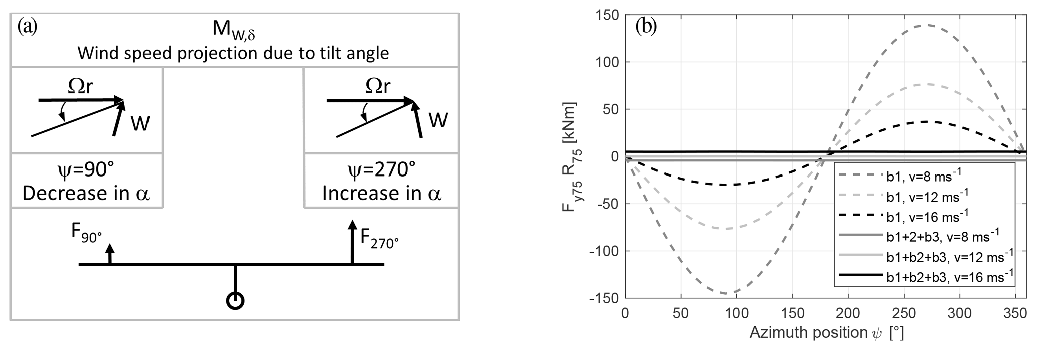
Figure 1 Aerodynamic yaw moment for the tilt angle of a downwind rotor sketched in (a) and the roughly estimated respective variation in yaw moment of the force at 75 % rotor radius with 5^∘ tilt in (b).

There are two yaw moment contributions due to the tilt angle. The first one is a projection of the main shaft torque, M_Q,δ, onto the yaw axis with the sine of the tilt angle (structural effect of tilt). As power production changes with wind speed, W, the yaw moment due to torque changes with wind speed. In the case of a yaw misalignment, the torque is reduced and influences the yaw moment accordingly. The second moment caused by the tilt angle M_W,δ is due to the wind speed projection, illustrated in Fig. 1 (aerodynamic effect of tilt, see Fig. 4 for angle definition). Figure 1a shows that the projection of the incoming wind speed is added to the relative velocity due to rotation ΩR when the blade moves up (azimuth range $\mathit{\psi }=\mathrm{0}{}^{\circ }$ to $\mathit{\psi }=\mathrm{180}{}^{\circ }$, azimuth position of $\mathit{\psi }=\mathrm{90}{}^{\circ }$ shown in Fig. 1) and subtracted from the rotational speed when the blade moves down (azimuth range $\mathit{\psi }=\mathrm{180}{}^{\circ }$ to $\mathit{\psi }=\mathrm{360}{}^{\circ }$, azimuth position of $\mathit{\psi }=\mathrm{270}{}^{\circ }$ shown in Fig. 1). The difference in projected wind speed due to the tilt angle creates a variation in angle of attack α over the azimuth position. Figure 1b shows the variation in the yaw moment over azimuth position for different wind speeds due to the force at 75 % of the rotor radius. It can be seen that the sum of the loading from three blades is not zero. In an attempt to isolate the effect of wind speed projection from tilt angle, the interaction with other effects, e.g. a combination of several angle projection (tilt angle, cone angle, and yaw) or the skewed inflow model for tilted inflow, are not included in the figure. The two tilt-dependent moments, M_Q,δ and M_W,δ, will cause a yaw misalignment for any free-yawing turbine with a structural tilt angle. An inclination angle of the wind field would also cause a moment from projections as M_W,δ.

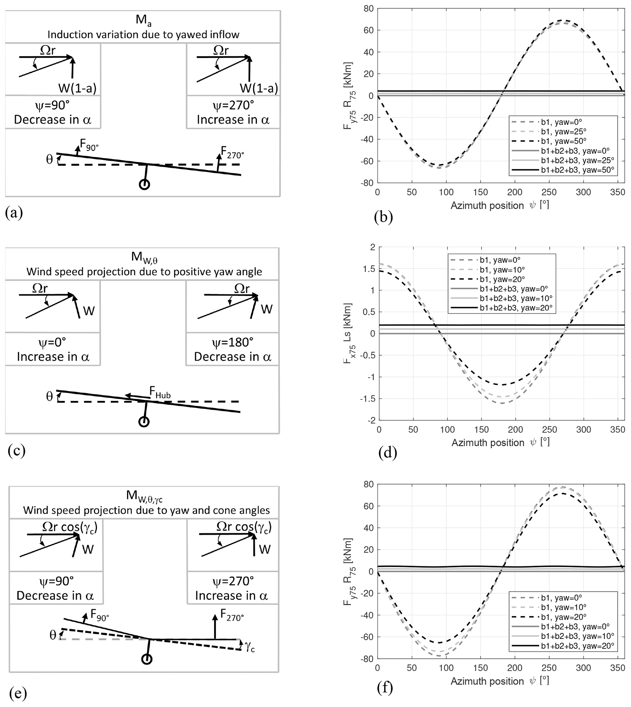
Figure 2 Aerodynamic mechanisms for yaw stiffness of a downwind rotor (a, c, e) and the roughly estimated respective variation in yaw moment of the force at 75 % rotor radius for wind speeds of 12 m s⁻¹ over azimuth position (b, d, f).

The moment due to induction variation over the rotor plane M_a, the moment due do wind speed projections from the a yaw angle M_W,θ, and the moment due to wind speed projections from a combination of yaw and cone angle $M_{W,{\mathit{\gamma }}_{\text{c}},\mathit{\theta }}$ are restorative moments. The restorative moments are creating an aerodynamic yaw stiffness as shown in Fig. 2. A yaw displacement will introduce a variation in induction over the rotor plane, due to the skewed inflow model, as one-half of the rotor is positioned deeper in the wake than the other half. The upstream-pointing blade is therefore loaded higher and a restoring yaw moment is created (Fig. 2a). It can be seen in Fig. 2b that relatively large yaw angles are required to create a significant restorative yaw moment from the variation in induction over the rotor plane compared to other stiffness mechanisms. An induction variation due to a skewed inflow is also created by the tilt angle. For a simple illustration of the main mechanisms, this effect is neglected here.

The positive yaw displacement, as shown in Fig. 2, creates a projection of the incoming wind speed. When the blade is pointing down ($\mathit{\psi }=\mathrm{0}{}^{\circ }$), the projected wind speed component is subtracted from the rotational speed, while it is added to the rotational speed when the blade is pointing up. The resulting variation in angle of attack is the reason for an in-plane force at the hub centre that creates a moment with the arm of the shaft length (Fig. 2c). This effect creates the smallest yaw moment of the discussed effects. However, with higher pitch angles, the contribution becomes larger at higher wind speeds, due to the flapwise force component that is projected to the in-plane forces.

In the case of coning, there is a difference in the projected wind speed between the left and the right side of the rotor when the rotor is yaw misaligned, resulting in a difference in angle of attack. From the difference in loading, a restoring yaw moment is created (Fig. 2e). It can be seen in Fig. 2f that relatively large yaw moments can be created for small yaw angles compared to the other two stiffness mechanisms, which makes the cone angle the most effective design parameter to influence the yaw stiffness.

Compared to the mechanical stiffness of a spring, the aerodynamic stiffness term does not necessarily create a restorative yaw moment. Negative force coefficient slopes over the angle of attack can create a negative stiffness term. In this case, any disturbance from the equilibrium point would increase the force moving the system away from the equilibrium point. An example would be the operation of the turbine during stall.

Figure 3 Aerodynamic mechanism for yaw damping for a downwind rotor.

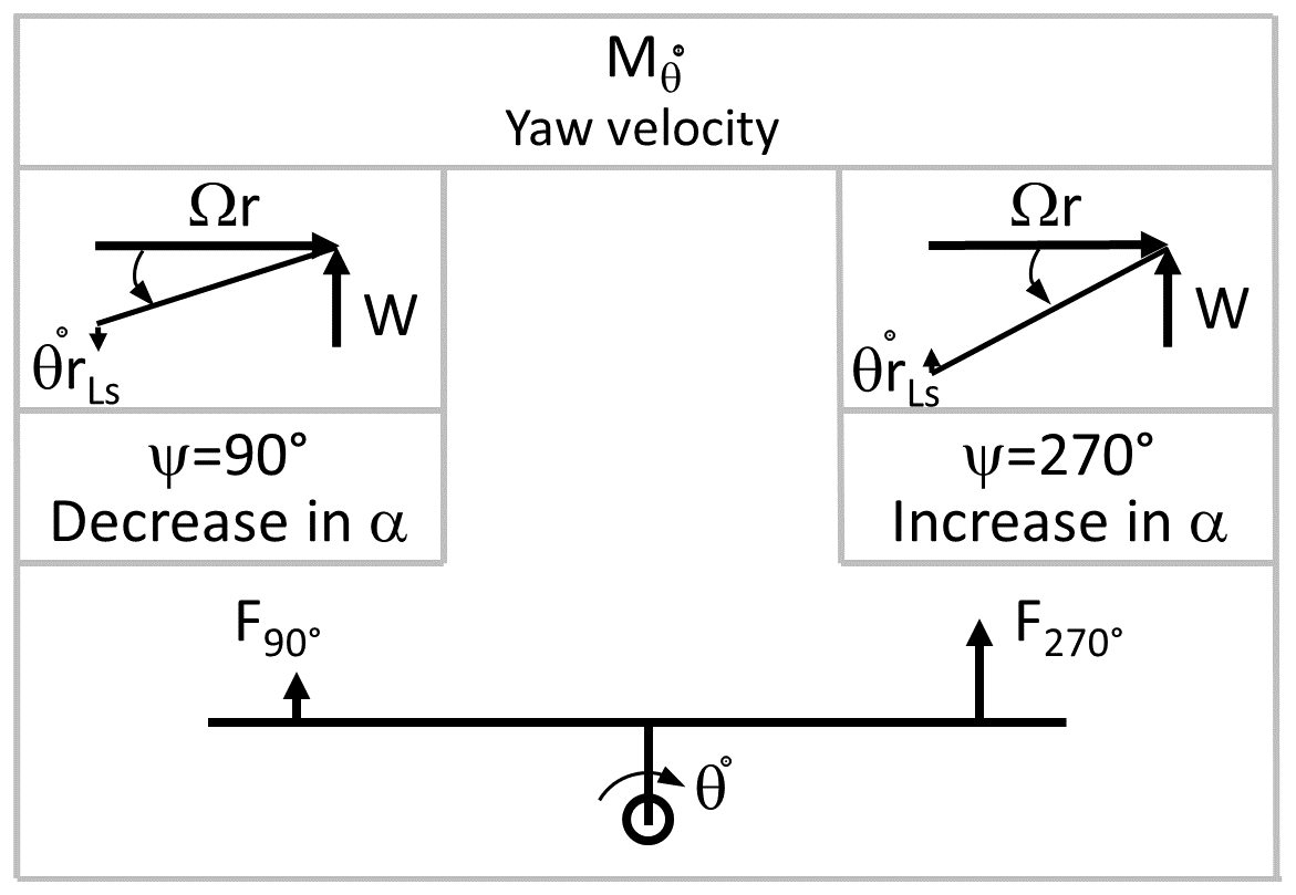
The damping mechanism for the free-yaw motion is shown in Fig. 3. The aerodynamic damping of the yaw motion is created by the rotational velocity due to the yawing motion. The rotational yaw velocity is added to the wind speed on one side of the rotor and subtracted on the other side of the rotor which leads to the change in angle of attack creating an imbalance in the loading that counteracts the yaw motion. Again, the created moment is only counteracting the yaw motion if the the slope of the airfoil coefficient over angle of attack is positive, i. e. operating in attached flow.

The stability of the equilibrium position of the yaw mode can be determined from the eigenvalue analysis of the system matrices. If the resulting real part of the eigenvalue λ is less than zero and the calculated eigenfrequency ω is non-zero, there is a positively damped yaw oscillation. If the real part of the eigenvalue and the eigenfrequency are larger than zero, the yaw equilibrium is unstable and the yaw motion is negatively damped (flutter, not to be confused with classical flutter). If the linear stiffness matrix for small yaw angles away from the equilibrium is negative, the system is driven away from the equilibrium without oscillations (divergence).

Flutter instability is given as

$$\mathrm{\Re }\left(\mathit{\lambda }\right)>\mathrm{0}\text{ and }\left|\mathit{\omega }\right|>\mathrm{0}$$

and divergence instability is given as

$$\mathrm{\Re }\left(\mathit{\lambda }\right)>\mathrm{0}\text{ and }\mathit{\omega }=\mathrm{0}.$$

2 Methods

This study focuses on two aspects. Firstly, the equilibrium yaw angle of a free-yawing turbine model which can align passively with the wind direction, and secondly the dynamic stability of the free-yaw mode. This study uses a simplified model of the Suzlon 2.1 MW turbine S111 (wind class IIIA). The original turbine has a three-bladed upwind rotor with a diameter of 112 m and a tower of 90 m height. The rotor is tilted 5^∘ and coned 3.5^∘. The turbine is operating at variable speed below rated power and is pitch regulated above the rated wind speed of 9.5 m s⁻¹ with a constant power approach. The operational range is between 4 and 21 m s⁻¹. In the investigation, the rotor configuration is changed to a downwind configuration. Thus, the rotor is shifted behind the tower, while nacelle and shaft are yawed by 180^∘. For the study, further simplifications are made. The blade geometry is modified: the prebend is neglected and quarter chord point of each airfoil is aligned on the pitch axis. The shaft intersects with the yaw axis. Figure 4 shows the simplified turbine model with the geometrical parameter shaft length (L_s) and distance to the centre of gravity (L_cg), tilt angle (δ), and cone angle (γ_c). These geometrical parameters will be used for a sensitivity study with regards to the equilibrium yaw angle and the dynamic stability of the free-yaw mode. All angles are sketched as positively defined for figures in this paper. The model is set up with two degrees of freedom (DOF) representing the free-yaw motion θ(t) and the tower side–side motion u_x(t) illustrated in Fig. 4. The ground fixed frame originates in the tower top centre. The distance between the origin and the centre of gravity of the nacelle assembly is L_cg and L_s represents the distance from the origin to the hub centre (shaft length). The hub length is r_h and z_b,k represents the position along the blade number k. The cone angle is denoted γ_c and δ is the tilt angle. The azimuth position of each blade is $\mathit{\psi }(k,t)=\mathrm{\Omega }t+\frac{\mathrm{2}\mathit{\pi }}{\mathrm{3}}(k-\mathrm{1})$, where Ω is the constant rotational speed of the shaft. The stiffness of the tower is represented by a linear spring with stiffness k_x. In Fig. 4d, a cross section of the blade is displayed with the inflow velocity U and the respective U_x and U_y components, the flow angle ϕ_k, and the pitch angle β_p, which includes the global blade pitch as well as the local twist. A steady wind field is assumed without shear, veer, inclination, turbulence, or tower shadow.

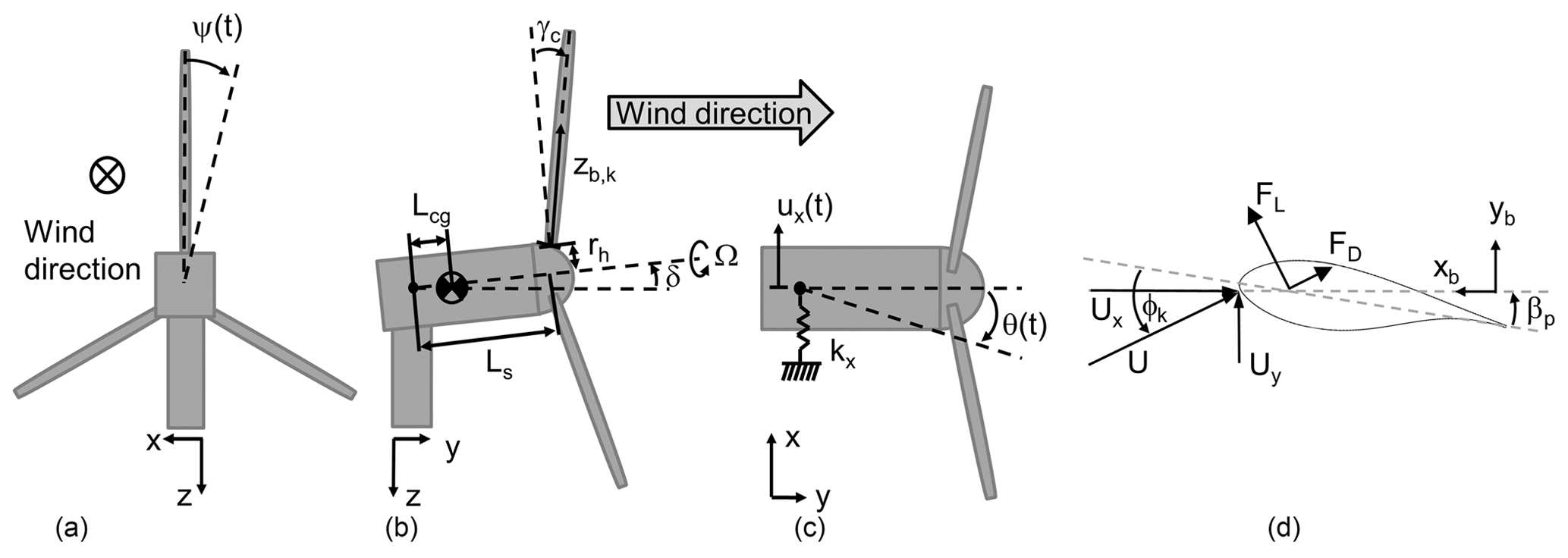
Figure 4 Schematics of turbine model and the according coordinate systems, front view (a), side view (b) and top view (c) and the sketch (d) of the inflow and forces on the airfoil with the coordinate system.

Figure 5 Flow chart for the implemented BEM code to compute the equilibrium yaw angle.

2.1 Equilibrium yaw angle

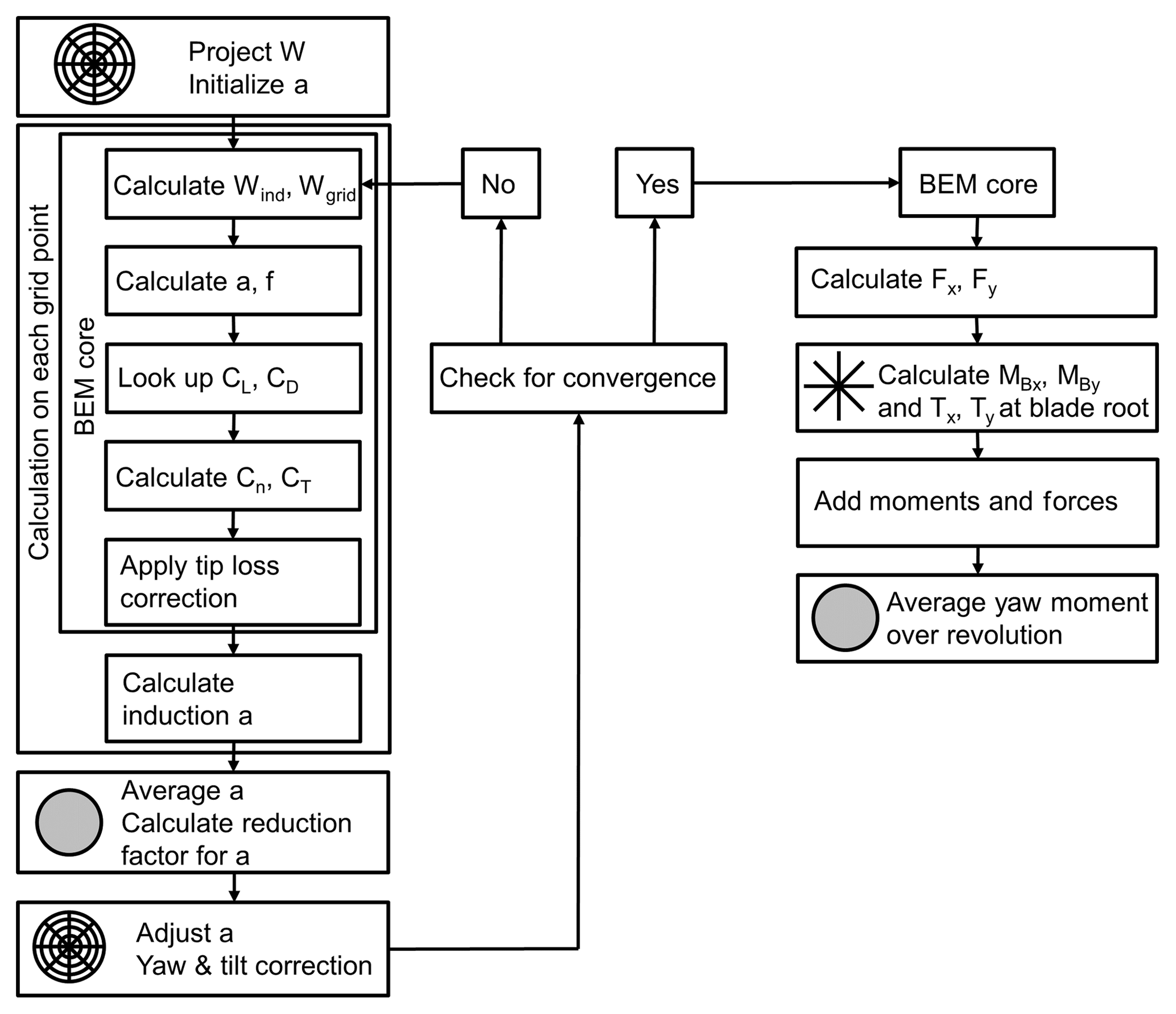
The equilibrium yaw angle, where the aerodynamic forces are in balance, is calculated with MATLAB (version 2018a). From a blade element momentum (BEM) code with yaw and tilt model, the forces on the rotor are calculated and the yaw angle associated with the zero-mean yaw moment on the yaw bearing is interpolated between the loading for different yaw angles, assuming that the effect of inertial terms is negligible. The BEM code is based on the aerodynamic module of the aeroelastic code HAWC2 (Larsen and Hansen, 2014). The basic principle of the induction varying over the rotor plane is briefly described in Madsen et al. (2011). Figure 5 shows the flow chart of the implemented BEM method. As in HAWC2, a polar grid is set up to define the calculation points for the induction. The free wind speed W is projected via a matrix rotation to the grid points, and the induction a is initialized. Within a converging loop the induced velocity W_ind and the actual velocity at each grid point W_grid are calculated. From the velocity the inflow angle ϕ and the angle of attack α are calculated. The lift and drag coefficients C_L and C_D are interpolated within a look-up table. From this the normal force coefficient C_n and the thrust coefficient C_T is calculated and the tip loss correction is applied. From the corrected thrust coefficient the new induction is calculated. The values are saved for each grid point and the average induction over all grid points is calculated. From the average induction a reduction factor is calculated. This factor is applied to each grid point to reduce the average induction according to the reduced thrust from the skewed inflow. Further, the local induction on each grid point is corrected according to the azimuth position of the blade by a yaw and a tilt factor. If the induction is then converged for all grid points within the requested tolerance, one more BEM-core operation is performed to calculate the force coefficients. From the force coefficients, the actual forces F_x and F_y are computed at the grid points. Those forces are integrated along the radial lines of the grid-to-blade-root bending moments $M_{{\text{B}}_x}$ and $M_{{\text{B}}_y}$, as well as to shear forces at the blade root T_x and T_y. The total yaw moment is calculated at the hub for a full revolution, extracting values from the calculation on the grid. The total moment contribution from the out-of-plane bending moments at the hub $M_{{\text{B}}_x,\mathit{\psi },\text{hub},\text{total}}$ is

$$\begin{array}{}\text{(1)}& M_{{\text{B}}_x,\mathit{\psi },\text{hub},\text{total}}=\sum _{k=\mathrm{1}}^{\mathrm{3}}{M}_{{\text{B}}_x,k}\sin \left({\mathit{\psi }}_k\right),\end{array}$$

where ψ_k is the azimuth position of the three individual blades, with ψ=0^∘ pointing downwards. It should be noted that there is a contribution to the yaw moment from the blade root bending moments, as well as from the shear forces, which have the shaft length as a distance to the centre of yaw rotation (see Fig. 2c). The total yaw moment is averaged over the rotor revolution. Finally, via interpolation, the equilibrium position is found. The equilibrium yaw position is the yaw angle where the average yaw moment is zero.

For the original turbine configuration, this method is validated with a HAWC2 simulation with a free-yawing turbine model without bearing friction. Thus, the rotor can align freely with the wind field. The wind field is steady, without shear, veer, inclination angle, or tower shadow model. The dynamic stall effects are neglected. The validated BEM code is then used for a parameter study, investigating the influence of tilt and cone angle, as well as the shaft length onto the equilibrium yaw angle of the turbine over wind speed. The operational conditions of the turbine are purely based on the free wind speed, neglecting any loss in power production due to skewed inflow.

2.2 Dynamic stability of the free-yaw mode

To evaluate the dynamic stability of the free-yaw mode, a simple 2-DOF model is set up in Maple software (MapleSoft, version 2016.2). The 2 degrees of freedom (2-DOF) model is based on an existing 15-DOF model without cone angle, described by Hansen (2003) and Hansen (2016). The 2 degrees of freedom are the tower side–side motion (u_x(t)) and the free-yaw motion (θ(t)). A 2-DOF model is chosen in the attempt to keep the model as simple and fast as possible. The advantage would be that such a model could, in principle, be used to make basic design choices very fast. The tower side–side motion is chosen as the second degree of freedom, as it couples directly to the yaw motion via the shaft length and the rotor mass. The model does not include structural damping or bearing friction. The tilt angle is assumed to be 0^∘ to align the rotor with the wind direction.

The governing equations of motion are set up from the Lagrange equation without structural damping

$$\begin{array}{}\text{(2)}& {\displaystyle \frac{\text{d}}{\text{d}t}}\left({\displaystyle \frac{\partial L}{\partial {\dot{x}}_i}}\right)-{\displaystyle \frac{\partial L}{\partial x_i}}=Q_i\text{for}i=\mathrm{1},\mathrm{2},\end{array}$$

where the Lagrangian $L=T-V$ is the difference between the kinetic energy T and the potential energy V and Q_i are the aerodynamic forces. The total kinetic energy can be written as

$$\begin{array}{ll}\text{(3)}& {\displaystyle }T=& {\displaystyle \frac{\mathrm{1}}{\mathrm{2}}}{m}_{\text{Na}}{\dot{\mathit{r}}}_{\text{cg,Na}}^{\mathrm{2}}+{\displaystyle \frac{\mathrm{1}}{\mathrm{2}}}{I}_z{\dot{\mathit{\theta }}}^{\mathrm{2}}+{\displaystyle \frac{\mathrm{1}}{\mathrm{2}}}\sum _{k=\mathrm{1}}^{\mathrm{3}}{m}_{\text{h}}{\dot{\mathit{r}}}_{\text{h},k}\cdot {\dot{\mathit{r}}}_{\text{h},k}{\displaystyle }& {\displaystyle }+{\displaystyle \frac{\mathrm{1}}{\mathrm{2}}}\sum _{k=\mathrm{1}}^{\mathrm{3}}\underset{\mathrm{0}}{\overset{R}{\int }}{m}_{\text{b}}{\dot{\mathit{r}}}_{\text{cg},k}\cdot {\dot{\mathit{r}}}_{\text{cg},k}\text{d}z,\end{array}$$

where m_Na represents the total mass of the nacelle and shaft; I_z is the total rotational inertia of the nacelle and shaft around the yaw axis; m_h is the total mass of the hub, represented as a point mass; and m_b is the distributed blade mass. The vectors r_cg,Na, r_h,k, and r_cg,k represent the position of the nacelle mass, the hub mass, and the blade centre of gravity, respectively, along the blade axis of the kth blade with the total length R and $\dot{\mathbf{\left(}\mathbf{\right)}}$ denotes their respective time derivative. These position vectors can be represented as

$$\begin{array}{}\text{(4)}& {\displaystyle }& {\displaystyle }{\mathit{r}}_{\text{cg,Na}}=\left[\begin{array}{c}{u}_x-\sin \left(\mathit{\theta }\right)L_{\text{cg}}\\ \cos \left(\mathit{\theta }\right)L_{\text{cg}}\\ \mathrm{0}\end{array}\right],\text{(5)}& {\displaystyle }& {\displaystyle }{\mathit{r}}_{\text{h},k}=\left[\begin{array}{c}{u}_x\\ \mathrm{0}\\ \mathrm{0}\end{array}\right]+{\mathbf{T}}_{\mathit{\theta }}\left(\left[\begin{array}{c}\mathrm{0}\\ L_{\text{s}}\\ \mathrm{0}\end{array}\right]+{\mathbf{T}}_{\mathit{\psi },k}\left[\begin{array}{c}\mathrm{0}\\ \mathrm{0}\\ r_{\text{h}}\end{array}\right]\right)\end{array}$$

and

$$\begin{array}{ll}\text{(6)}& {\displaystyle }{\mathit{r}}_{\text{cg},k}& {\displaystyle }=\left[\begin{array}{c}{u}_x\\ \mathrm{0}\\ \mathrm{0}\end{array}\right]{\displaystyle }& {\displaystyle }+{\mathbf{T}}_{\mathit{\theta }}\left(\left[\begin{array}{c}\mathrm{0}\\ L_{\text{s}}\\ \mathrm{0}\end{array}\right]+{\mathbf{T}}_{\mathit{\psi },k}\left(\left[\begin{array}{c}\mathrm{0}\\ \mathrm{0}\\ r_{\text{h}}\end{array}\right]+{\mathbf{T}}_{{\mathit{\gamma }}_{\text{c}}}\left[\begin{array}{c}\mathrm{0}\\ \mathrm{0}\\ z\end{array}\right]\right)\right).\end{array}$$

It should be noted that the centre of gravity of the blade sections is assumed to be aligned on a straight line for simplicity. The rotation matrices for yaw T_θ, rotor rotation ${\mathbf{T}}_{{\mathit{\psi }}_k}$ and the cone angle ${\mathbf{T}}_{{\mathit{\gamma }}_{\text{c}}}$ are defined according to the right-hand rule, as

$$\begin{array}{ll}\text{(7)}& {\displaystyle }& {\displaystyle }{\mathbf{T}}_{\mathit{\theta }}=\left[\begin{array}{ccc}\cos \left(\mathit{\theta }\right)& -\sin \left(\mathit{\theta }\right)& \mathrm{0}\\ \sin \left(\mathit{\theta }\right)& \cos \left(\mathit{\theta }\right)& \mathrm{0}\\ \mathrm{0}& \mathrm{0}& \mathrm{1}\end{array}\right],{\displaystyle }& {\displaystyle }{\mathbf{T}}_{{\mathit{\psi }}_k}=\left[\begin{array}{ccc}\cos \left({\mathit{\psi }}_k\right)& \mathrm{0}& \sin \left({\mathit{\psi }}_k\right)\\ \mathrm{0}& \mathrm{1}& \mathrm{0}\\ -\sin \left({\mathit{\psi }}_k\right)& \mathrm{0}& \cos \left({\mathit{\psi }}_k\right)\end{array}\right],\\ {\displaystyle }& {\displaystyle }{\mathbf{T}}_{{\mathit{\gamma }}_{\text{c}}}=\left[\begin{array}{ccc}\mathrm{1}& \mathrm{0}& \mathrm{0}\\ \mathrm{0}& \cos \left({\mathit{\gamma }}_{\text{c}}\right)& \sin \left({\mathit{\gamma }}_{\text{c}}\right)\\ \mathrm{0}& -\sin \left({\mathit{\gamma }}_{\text{c}}\right)& \cos \left({\mathit{\gamma }}_{\text{c}}\right)\end{array}\right],\end{array}$$

where the cone angle is a negative rotation for a positive cone angle.

The potential energy V is formulated in the general manner, including a yaw stiffness as

$$\begin{array}{}\text{(8)}& V={\displaystyle \frac{\mathrm{1}}{\mathrm{2}}}{k}_x{u}_x^{\mathrm{2}}+{\displaystyle \frac{\mathrm{1}}{\mathrm{2}}}{G}_z{\mathit{\theta }}^{\mathrm{2}},\end{array}$$

where G_z is the yaw stiffness, which will be set to G_z=0 Nm⁻¹ for the analysis of the free-yawing turbine. Inserting the Lagrangian L into Eq. (2) and linearization about the equilibrium position at the steady state ($\mathit{x}=\dot{\mathit{x}}=\mathrm{0}$) gives the structural part of the linear equation of motion. The linearization around a steady state of x=0 assumes that there exists an equilibrium position where the rotor is fully aligned with the wind direction, as the tilt angle is 0^∘. From the linearized model, the stability due to small angle variations around the equilibrium can be investigated. It can be seen from Fig. 4d that the relative inflow velocity at the blade U_k, the inflow angle ϕ_k, and the angle of attack α_k are

$$\begin{array}{ll}{\displaystyle }& {\displaystyle }{U}_k=\sqrt{U_{x,k}^{\mathrm{2}}+U_{y,k}^{\mathrm{2}}},\\ \text{(9)}& {\displaystyle }& {\displaystyle }{\mathit{\varphi }}_k=\arctan \left({\displaystyle \frac{U_{y,k}}{U_{x,k}}}\right),{\displaystyle }& {\displaystyle }{\mathit{\alpha }}_k={\mathit{\varphi }}_k-{\mathit{\beta }}_{\text{p}},\end{array}$$

where β_p includes the pitch angle and the local twist. For simplicity, it is assumed that the aerodynamic centre r_ac,k is coinciding with the centre of gravity on a straight line, the z_b axis. The vector of the relative velocity is defined as

$$\begin{array}{}\text{(10)}& \mathit{U}={\left({\mathbf{T}}_{\mathit{\theta }}{\mathbf{T}}_{{\mathit{\psi }}_k}{\mathbf{T}}_{{\mathit{\gamma }}_{\text{c}}}\right)}^{-\mathrm{1}}\left({\dot{\mathit{r}}}_{\text{ac},k}-\left[\begin{array}{c}\mathrm{0}\\ W\\ \mathrm{0}\end{array}\right]\right),\end{array}$$

where W is the incoming undisturbed wind to the rotor plane.

The resulting forces in the global coordinate frame can be read as

$$\begin{array}{}\text{(11)}& {\mathit{F}}_{\mathit{k}}(z,\mathit{x},\dot{\mathit{x}})={\mathbf{T}}_{\mathit{\theta }}{\mathbf{T}}_{{\mathit{\psi }}_k}{\mathbf{T}}_{{\mathit{\gamma }}_{\text{c}}}\left[\begin{array}{c}{f}_x(z,\mathit{x},\dot{\mathit{x}})\\ f_y(z,\mathit{x},\dot{\mathit{x}})\\ \mathrm{0}\end{array}\right],\end{array}$$

where the aerodynamic force components f_x and f_y are combined from the lift and drag coefficients as

$$\begin{array}{ll}{\displaystyle }{f}_x=& {\displaystyle \frac{\mathrm{1}}{\mathrm{2}}}\mathit{\rho }c{U}_k^{\mathrm{2}}(z,\mathit{x},\dot{\mathit{x}})\left(C_{\text{L}}\left({\mathit{\alpha }}_k\right(z,\mathit{x},\dot{\mathit{x}}\left)\right)\sin {\mathit{\varphi }}_k(z,\mathit{x},\dot{\mathit{x}})\right.\\ \text{(12)}& {\displaystyle }& {\displaystyle }\left.-C_{\text{D}}\left({\mathit{\alpha }}_k\right(z,\mathit{x},\dot{\mathit{x}}\left)\right)\cos {\mathit{\varphi }}_k(z,\mathit{x},\dot{\mathit{x}})\right),{\displaystyle }{f}_y=& {\displaystyle \frac{\mathrm{1}}{\mathrm{2}}}\mathit{\rho }c{U}_k^{\mathrm{2}}(z,\mathit{x},\dot{\mathit{x}})\left(C_{\text{L}}\left({\mathit{\alpha }}_k\right(z,\mathit{x},\dot{\mathit{x}}\left)\right)\cos {\mathit{\varphi }}_k(z,\mathit{x},\dot{\mathit{x}})\right.\\ {\displaystyle }& {\displaystyle }\left.+C_{\text{D}}\left({\mathit{\alpha }}_k\right(z,\mathit{x},\dot{\mathit{x}}\left)\right)\sin {\mathit{\varphi }}_k(z,\mathit{x},\dot{\mathit{x}})\right),\end{array}$$

where ρ is the air density and C_L and C_D are the lift and drag coefficients, respectively.

Inserting the time derivative of Eq. (6) representative for ${\dot{\mathit{r}}}_{\text{ac}\mathbf{,}\mathit{k}}$ and Eqs. (11) and (9) to Eqs. (10) and (12) and linearization around the steady state gives the linear aerodynamic matrices in the form of

$$\begin{array}{}\text{(13)}& \mathit{Q}=-{\mathbf{C}}_{\text{aero}}\dot{\mathit{x}}-{\mathbf{K}}_{\text{aero}}\mathit{x},\end{array}$$

where the aerodynamic forces Q have no constant component and result in the aerodynamic damping matrix C_aero and the aerodynamic stiffness matrix K_aero.

Here, the velocity triangle in the steady state is inserted with the components of U₀, as shown in Fig. 4d,

$$\begin{array}{}\text{(14)}& U_{\mathrm{0}x}=\mathrm{\Omega }\left(r_{\text{h}}+z\right)\cos \left({\mathit{\gamma }}_{\text{c}}\right),U_{\mathrm{0}y}=W\cos \left({\mathit{\gamma }}_{\text{c}}\right).\end{array}$$

For simplicity in the derivation of the governing model, the induction is neglected in the upper equation. All resulting matrices can be found in Appendix B.

From the upper equations (Eqs. 2, 3, 8, and 13) a system matrix A can be defined as

$$\begin{array}{}\text{(15)}& \mathbf{A}=\left[\begin{array}{cc}\mathbf{0}& \mathbf{I}\\ {\mathbf{M}}^{-\mathrm{1}}\left({\mathbf{K}}_{\text{struc}}+{\mathbf{K}}_{\text{aero}}\right)& {\mathbf{M}}^{-\mathrm{1}}\left({\mathbf{C}}_{\text{aero}}\right)\end{array}\right],\end{array}$$

where M is the mass matrix, K_struc and K_aero are the structural and aerodynamic stiffness matrices, C_aero is the aerodynamic damping matrix, and I is the identity matrix. The real parts of the eigenvalues of the upper system matrix (Eq. 15) determine the damping of the system.

A steady simple BEM code (referred to as the “simple BEM code”) is used in MATLAB (R2018a), to determine the force coefficients along the blade span and to include the induction in the inflow velocity on the airfoil. The simple BEM code does not include skewed inflow models due to yaw or tilt. The induction is calculated along the rotor radius only since there is no dependency of the induction on the azimuth position. The structural stiffness of the tower is tuned to account for the neglected mass distribution of the tower. Eigenanalysis of the system matrix is performed in MATLAB over a range of wind speeds, and the real parts of the eigenvalue of the yaw mode are evaluated.

For the turbine configuration with the original cone, length, and mass distribution, the 2-DOF model is imitated in the aeroelastic modal analysis tool HAWCStab2, described by Hansen (2004). Stiff turbine components are modelled except that the tower side–side bending and the yaw bearing are free to rotate. The real parts of the eigenvalues are compared to validate the results from the 2-DOF model.

The validated model is used for a parameter study to investigate the influence of geometrical turbine parameter on the real part of the yaw mode eigenvalue. The varied parameter are the cone angle, the shaft length, and the position of the centre of gravity of the nacelle along the shaft.

Finally, HAWCStab2 is used to investigate if the stability limit of the yaw mode would occur within the normal operational wind speed range of the turbine and which further degrees of freedom, additional to the tower side–side and yaw, would be needed to predict instability.

3 Results

The following section shows the results for the equilibrium yaw angle and the stability of the yaw mode.

3.1 Equilibrium yaw angle

Figure 6 shows the comparison of the equilibrium yaw angle found by HAWC2 and the equilibrium yaw angle found from the BEM code (Fig. 5) over the wind speed for the original turbine configuration with 5^∘ tilt and 3.5^∘ cone.

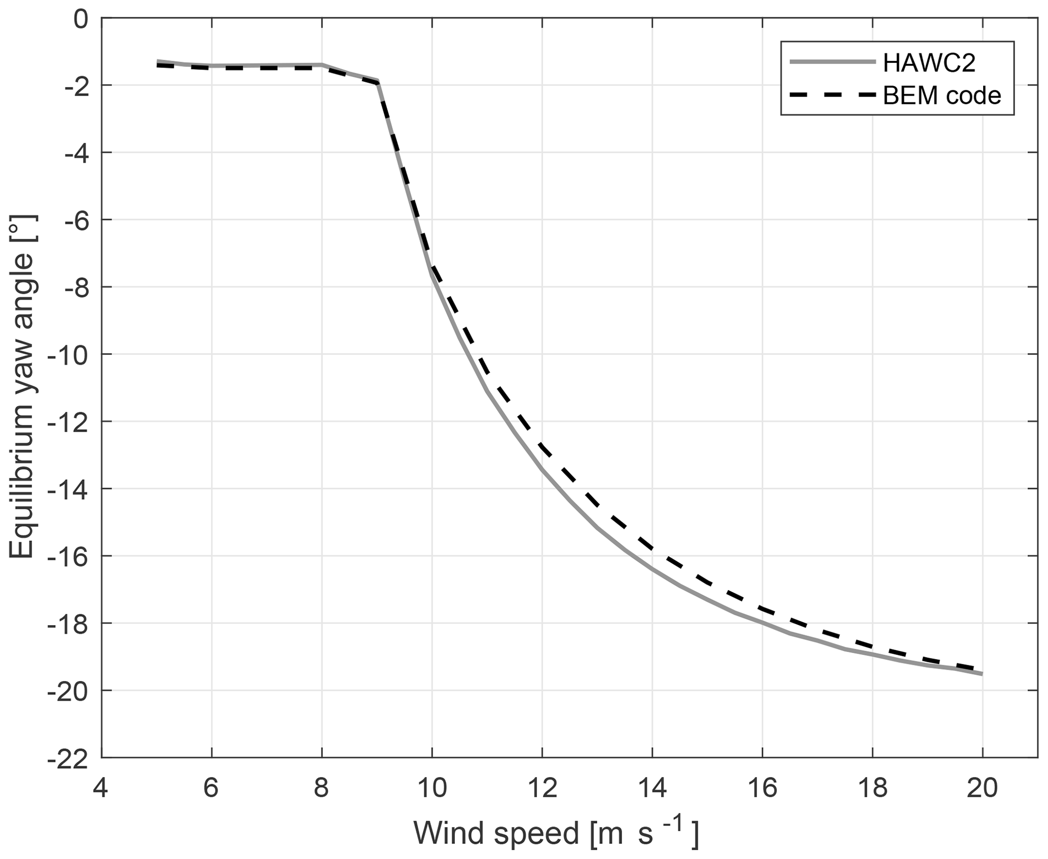
Figure 6 Comparison of the equilibrium yaw angle over wind speed from HAWC2 and the BEM code for the original turbine configuration with 5^∘ tilt and 3.5^∘ cone.

The figure shows that the equilibrium angle is not zero. The equilibrium yaw angle is constant at −1.4^∘ from cut-in wind speed up to 8 m s⁻¹. Between 8 m s⁻¹ and below rated wind speed (9 m s⁻¹) the equilibrium yaw angle decreases slightly to −1.8^∘. For wind speeds higher than the rated wind speed (9.5 m s⁻¹), the equilibrium yaw angle decreases strongly. The slope of the equilibrium yaw angle over wind speed changes so that the equilibrium yaw angle shows a tendency to asymptotically reach a minimum. The lowest observed equilibrium yaw angle of −19.4^∘ is reached at 20 m s⁻¹. The equilibrium yaw angle calculated by HAWC2 and with the BEM code differ with a maximum of 0.6^∘ at around 13 m s⁻¹.

The analysis shows that there will be a yaw moment even with a perfect alignment of the rotor with the wind direction, which drives the rotor to the non-zero equilibrium angle. This yaw moment is due to the tilt angle. Including a tilt angle has two effects. Aerodynamically, the projection of the global wind speed leads to a yaw moment as illustrated in Fig. 1. Structurally, the tilt leads to a yaw moment as the torque axis is not perpendicular to the yaw axis and the torque M_Q is projected to the yaw axis with sin (δ)M_Q. While the structural effect follows the torque curve, the aerodynamic effect is influenced by the rotor speed and increases with the wind speed. When the rotor is free to align with the wind direction, the moment due to tilt pushes the rotor to a non-zero yaw position. At a non-zero yaw position a restorative yaw moment is present due to yaw stiffness (see Fig. 2). The rotor finds a new equilibrium yaw angle. As the equilibrium yaw angle between HAWC2 and the BEM code agree well, the BEM code is therefore used for the parameter study.

Figure 7 shows the equilibrium yaw angle (panel a) and the relative power production (panel b) depending on the tilt angle and wind speed.

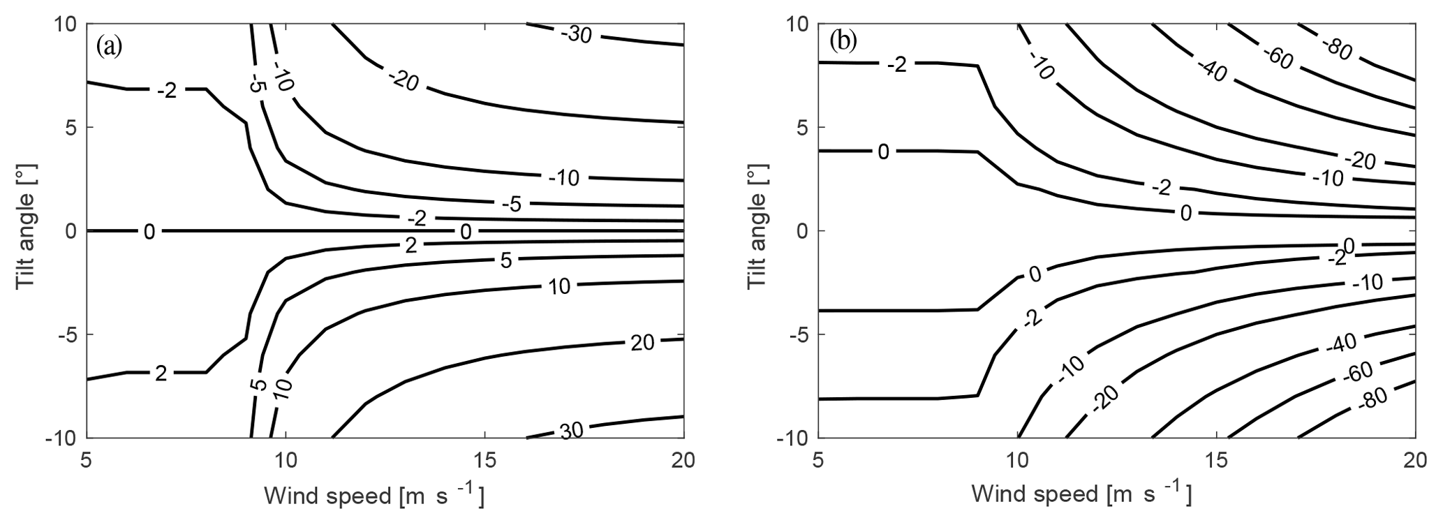
Figure 7 Equilibrium yaw angle (^∘) (a) and the relative difference in power production (%) (b) depending on tilt angle and wind speed variation for a turbine configuration with 3.5^∘ cone. The relative, difference in power is compared at each calculation point relative to the power production of the original turbine, with a forced yaw alignment.

A zero tilt angle will give a zero equilibrium yaw angle, which means a full alignment of the rotor with the wind direction. Negative tilt angles show a positive equilibrium yaw angle and positive tilt angles show a negative equilibrium yaw angle. The dependency of the equilibrium yaw angle on the tilt angle is stronger for higher wind speeds. The relative power difference shows the highest losses for extreme tilt angles and high wind speeds. There is zero relative power difference at zero tilt angle.

There is no yaw moment for yaw alignment of the rotor plane with the wind direction if there is a zero tilt angle. As a yaw moment due to a tilt angle is dependent on the sine of the tilt angle, the equilibrium yaw angle is anti-symmetric around the line of full alignment (0^∘). With larger tilt angles, a larger yaw moment is created aerodynamically and structurally. The larger yaw moment drives the rotor to larger equilibrium yaw angles, where a counteracting yaw moment is created from the imbalance of forces by the induction variation and wind speed projections from yaw and cone angles. The power production shows the expected behaviour for a non-perpendicular inflow to the rotor plane. The higher the equilibrium yaw angle is, the lower the wind speed component perpendicular to the rotor plane, the lower the power production, and the higher the difference to the reference power curve are.

Figure 8 shows the equilibrium yaw angle (panel a) and the relative difference in power production (panel b) for the variation of cone and wind speed. The figure is stitched together at the grey line, as the calculated data showed an inconsistency. Here the angles tend to increase to very large positive and negative angles rather than decrease to zero as a continuous figure would suggest.

Figure 8 Equilibrium yaw angle (^∘) (a) and the relative difference in power production (%) (b) depending on cone angle and wind speed variation for a turbine configuration with 5^∘ tilt. The figure is stitched together from two sub-figures at the grey line.

Figure 8a shows that cone angles higher than 0^∘ give a negative equilibrium yaw angle, while cone angles lower than −2.5^∘ give a positive equilibrium yaw angle. It can also be seen that highly positive, as well as highly negative, cone angles give equilibrium yaw angles closer to zero and a smaller variation in the equilibrium yaw angle over wind speed. The higher the wind speed and the closer the wind speed to the stitching line, the larger and more positive or negative are the calculated equilibrium yaw angles. Figure 8b shows that the extreme equilibrium yaw angles come with an extreme power loss. The negative cone angles combined with the positive equilibrium yaw angles at low wind speed are associated with a higher power loss than the combination of negative equilibrium yaw angles and positive cone angles.

Varying the cone angle for the tilted turbine configuration has an effect on the torque. A larger cone angle reduces the torque, which leads to a reduced projected yaw moment due to the tilt M_Q,δ. The aerodynamic moment M_W,δ due to tilt, on the other hand, is hardly influenced. Further, larger cone angles increase the yaw moment due to yawed inflow on the coned rotor $M_{W,\mathit{\theta },{\mathit{\gamma }}_{\text{c}}}$ (see Fig. 2e). Thus, for larger positive cone angles, a smaller equilibrium angle is found, not just due to the increased stiffness from cone but also due to a smaller moment from the tilt angle M_Q,δ. For larger negative cone angles, the moment due to coned and yawed inflow is only counteracting the moments due to tilt if the rotor is aligned with a yaw error of the opposite sign. Otherwise the stiffness from yawed and coned inflow would be negative and the force would not be restorative (see Fig. 2e). As the stiffness for yawed and coned inflow is becoming very small for small cone angles, the yaw moment due to tilt has to be balanced by the moment due to induction variation M_a (see Fig. 2a) and due to yawed inflow M_W,θ (see Fig. 2c). As the two moments M_a and M_W,θ need larger yaw angles to create a significant yaw moment, the equilibrium yaw angle becomes large for small cone angles (compare Fig. 2b, d, f). Due to three-dimensional effects of the wind speed projection, the aerodynamic yaw moment due to tilt M_W,δ is not symmetric for cone angles around zero. Compared to the estimated yaw moment of the airfoil at R=0.75 % for 16 m s⁻¹ and 5^∘ tilt in Fig. 1, the difference between a positive and a negative cone angle (±0.5^∘) is around 12 %. As a sum the total yaw moment due to tilt is slightly different for negative and positive cone angles, and the asymmetry in Fig. 8 is observed. Since the equilibrium yaw moment is not symmetric around zero, the negative cone angles combine with higher positive equilibrium yaw angles, so there is a higher power loss for negative cone angles than for positive cone angles.

Figure 9 shows the equilibrium yaw angle (panel a) and the relative power difference (panel b) over wind speed and the shaft length factor. This factor is directly multiplied with the shaft length to increase or decrease the absolute shaft length.

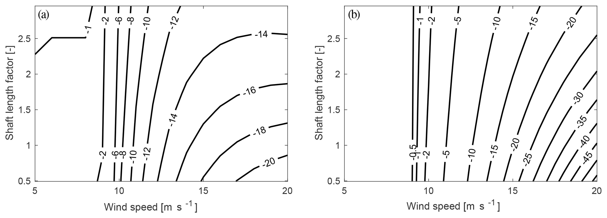
Figure 9 Equilibrium yaw angle (^∘) (a) and the relative difference in power production (%) (b) depending on shaft length and wind speed variation for a turbine configuration with 5^∘ tilt and 3.5^∘ cone. The relative, difference in power is compared at each calculation point relative to the power production of the original turbine, with a forced yaw alignment.

Figure 9a shows that the shaft length factor has nearly no influence on the equilibrium yaw position for low wind speeds. Only for high wind speeds above rated power, the equilibrium yaw angle is higher for smaller shaft length factors than for small shaft length factors. As shown on the right, the relative difference in power is hardly influenced by the shaft length factor. Only for high wind speeds, less power loss is observed for higher shaft length factors than for lower shaft length factors.

As discussed previously the shaft length acts as the moment arm for the summed in-plane shear forces on the hub. For the in-plane shear forces to be significantly large, a large yaw angle and high wind speeds are required to create an imbalance on the angle of attack between the upper and the lower rotor halves (see Fig. 2c). Only in this case the moment created from the force at the hub and the shaft length as the moment arm is large enough to partly counteract the moment created by the tilt angle. However, within the range of investigated wind speeds, the yaw misalignment with the wind direction is still so large that hardly any power difference can be recovered by the investigated increase in shaft length.

3.2 Dynamic stability of the free-yaw mode

The following section discusses the stability of the free-yaw mode of the turbine for a tilt angle of 0 and 3.5^∘ cone angle. The free-yaw motion is stable around the equilibrium point if it is positively damped, which means that the real part of the two eigenvalues for the yaw mode are negative. Figure 10 shows the comparison of the real parts of the eigenvalue of the yaw mode of the analytic 2-DOF model and the imitation in HAWCStab2.

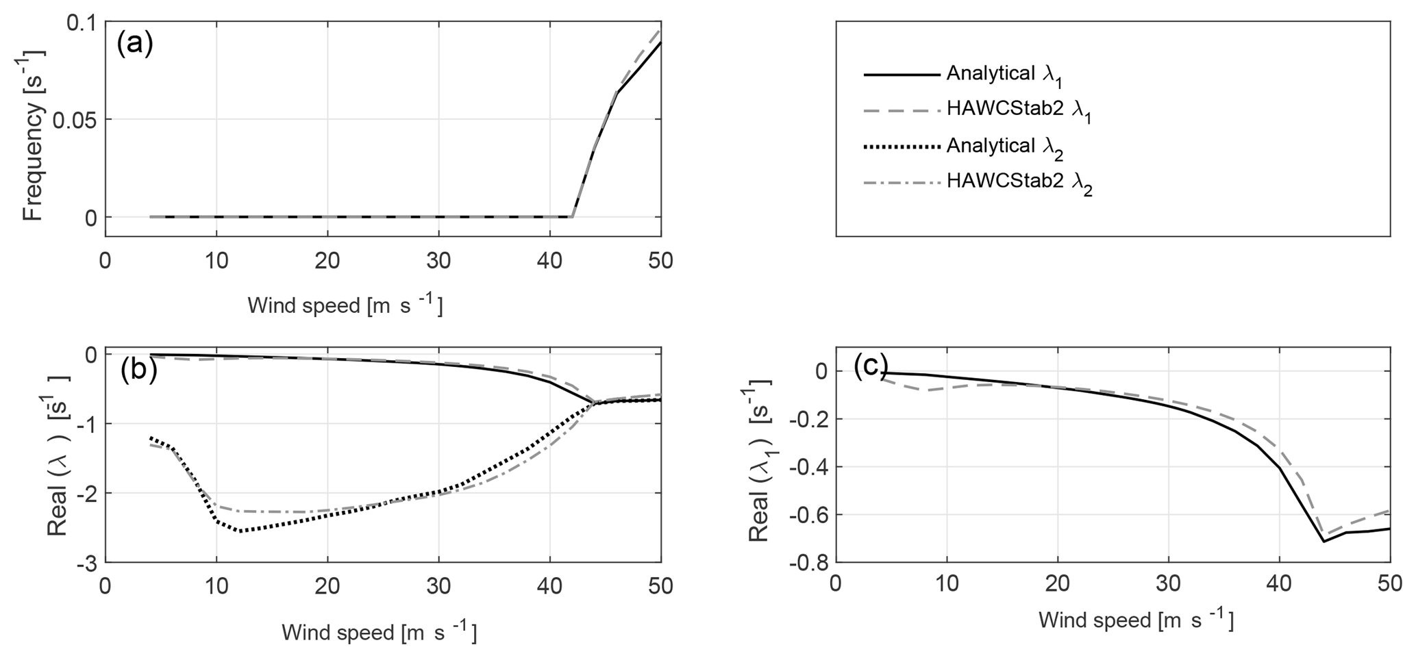
Figure 10 Comparison of the frequency (a), the real part of the two eigenvalues (b) and a zoom into the first eigenvalue (c) of the yaw mode for the 2-DOF model from the analytic solution, and the imitation in HAWCStab2.

It can be seen at the top of the figure that there is a yaw frequency of zero up to a wind speed of 42 m s⁻¹. For higher wind speeds, the frequency is increasing up to 0.9 s⁻¹ at 50 m s⁻¹ for the solution from HAWCStab2. The results of the analytic 2-DOF model and the imitation in HAWCStab2 differ by a maximum of 0.01 s⁻¹ in the computation of the frequency of the free-yaw mode. At the bottom of the figure, the real parts of the complex pair of eigenvalues is displayed in Fig. 10b, and a zoom for the real part of the first eigenvalue is displayed in Fig. 10c. The real part of the first and second eigenvalues are equal only for non-zero frequencies. The first eigenvalue is generally closer to zero than the second eigenvalue for wind speeds below 44 m s⁻¹. The first eigenvalue decreases for wind speeds up to 8 m s⁻¹. The slope of the eigenvalue over wind speed changes for wind speeds above rated power. The second eigenvalue decreases to a minimum at 10 m s⁻¹ for HAWCStab2 and at 12 m s⁻¹ for the analytical 2-DOF model. For higher wind speeds, the second eigenvalue increases. The total eigenvalue increases for wind speeds of 44 m s⁻¹ and higher. For any negative real part of the eigenvalue and zero frequency (wind speeds below 44 m s⁻¹), a small displacement will initiate the motion back to the equilibrium point without oscillation (convergence). For wind speeds of 44 m s⁻¹ and higher, there will be an oscillatory motion that will decrease in amplitude until the rotor aligns at the equilibrium position. The difference between the solution of HAWCStab2 and from the analytical model is up to 0.08 s⁻¹ for the first eigenvalue and up to 0.5 s⁻¹ for the second eigenvalue. The analytical 2-DOF model and the imitation in HAWCStab2 cannot be expected to give the same results, since the HAWCStab2 model includes the rolling motion of the nacelle and the motion of the distributed tower mass instead of a lumped point mass. However, the real parts of the first eigenvalues of the two models are close so that the analytical model can be used for the parameter study. The results of the parameter study will be sufficient to identify the parameters that stabilize or destabilize the free-yawing motion of the turbine.

Including the aerodynamic forces to the mechanical system has two effects. Firstly, there is an aerodynamic stiffness, due to the mechanisms of wind speed projection as shown in Fig. 2. The effect of induction variation is negligible for small yaw angles. Secondly, the yaw motion creates a flow velocity that is added to the wind speed on one side of the rotor and subtracted from the wind speed on the other side of the rotor (Fig. 3), which again changes the angle of attack and therefore the aerodynamic forces create a moment which dampens the yaw motion.

The main influence can be observed from the slope of the lift coefficients if the outputs from the simple BEM code are manually manipulated for the eigenanalysis. As the yaw moment for moderate pitch angles is dominated by the flapwise forces, the drag and the slope of the drag coefficient are of minor influence. As the projection of the forces changes with the pitch angle, a clear dependency on the wind speed can be observed and also the change in the slope of the real part of the eigenvalue can be observed at the rated wind speed. Further, the operational point changes so the force coefficients and their slopes are expected to change the eigenvalues over wind speed.

Figure 11 shows the real parts of the first (panel a) and of the second (panel b) eigenvalue over the variation in cone angle and wind speed.

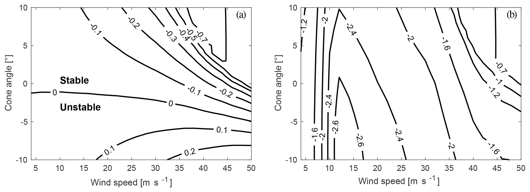
Figure 11 Real part of the first (a) and second (b) eigenvalue of the yaw mode for a variation in cone angle and wind speed from the 2-DOF model.

The figure shows that the real part of the first eigenvalue changes sign and becomes positive for cone angles of −1^∘ at 4 m s⁻¹ and −5^∘ at 50 m s⁻¹. Thus, the zero equilibrium position becomes unstable for these negative cone angles. It can also be seen that large, positive cone angles decrease the real part of the first eigenvalue and therefore increase the damping. The larger the wind speed, the larger the effect of variation in the cone angle on the real part of the first eigenvalue. The real part of the second eigenvalue is influenced less than the real part of the first eigenvalue and varies mainly with wind speed. For very high cone angles, the minimum real part is slightly increased by 0.2 s⁻¹ at around 14 m s⁻¹. Extremely high wind speeds, larger than 40 m s⁻¹, show an increase in the real part of the second eigenvalue for very high cone angles. The imaginary part in the unstable region is zero, indicating a divergence instability. In the stable region, the imaginary part of the eigenvalues is the same for high wind speeds (higher 42 m s⁻¹) and high cone angles, which means that there is a positively damped oscillatory yaw motion (flutter).

The cone angle mainly affects the aerodynamic stiffness, as shown in Fig. 2. The damping is hardly effected. However, as discussed previously, the negative cone angles can create a negative stiffness driving the system away from the equilibrium position. A positive damping coefficient in the damping matrix cannot restore the equilibrium position in this case and the real part of the eigenvalue becomes positive. As high velocities create a positive stiffness component from the in-plane forces and due to the shaft length, the instability does not occur at zero cone angle and can tolerate slightly more negative cone angles at high wind speeds.

Figure 12 shows the real part of the first (panel a) and second (panel b) eigenvalue over a variation in wind speed and shaft length.

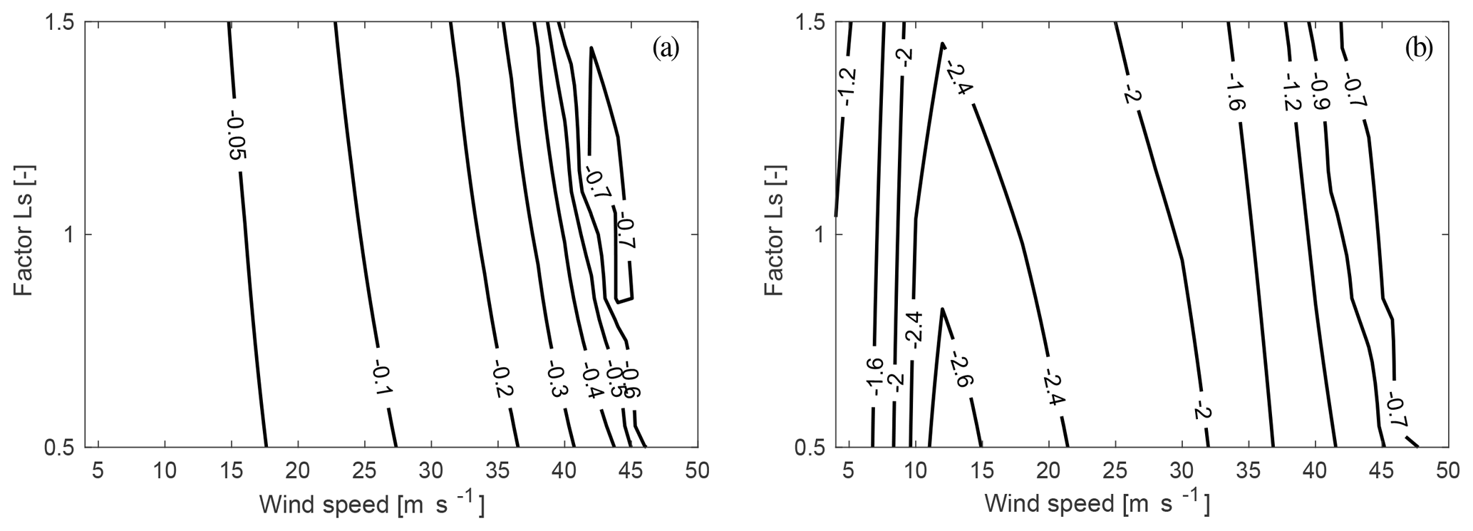
Figure 12 Real part of the first (a) and second (b) eigenvalue of the yaw mode for a variation in shaft length and wind speed from the 2-DOF model.

It can be seen that the real parts of the eigenvalues hardly change with variation in the shaft length. A lower shaft length slightly increases the real part of the eigenvalue. High shaft length slightly decreases the minimum of the second eigenvalue at around 14 m s⁻¹.

Large shaft lengths can increase the projected wind speed for the damping term, as the centre of rotation is far away from the rotor plane. However, as realistic values of the shaft length are always much lower than the blade length, the influence on the damping is very low. Also, the influence on the stiffness can hardly be observed, as the effect of in-plane forces is very small for small yaw angles (linearization point of 0^∘ yaw). Overall, this leads to the fact that the eigenvalue of the yaw mode is hardly influenced by the shaft length within the investigated range.

A figure for the real parts of the eigenvalue changing with the position of the centre of gravity is not shown. The distance of the centre of gravity only effects the rotational inertia for the yaw motion. As the stiffness and damping are not effected, the real part of the eigenvalues are hardly changing from eigenanalysis of the system matrix.

Figure 13 shows the frequency at the top and at the bottom the real part of the first eigenvalue of the free-yaw mode from HAWCStab2 over wind speeds. In the figure, the 2-DOF imitation, the extension of the 2-DOF imitation with flapwise blade flexibility, the extended 2-DOF model with updated steady state (deformed blade including prebend), and the full turbine model are compared.

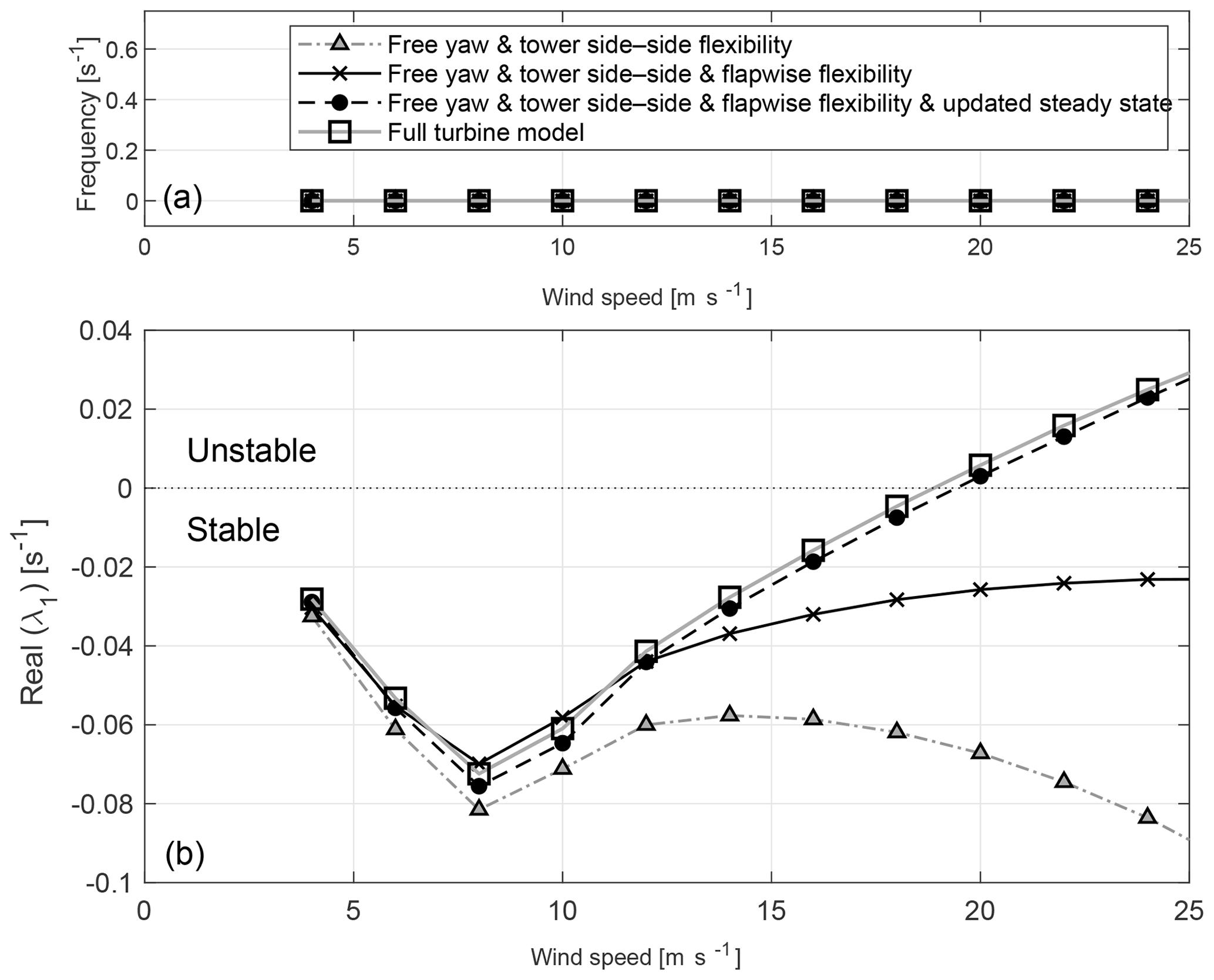
Figure 13 Comparison of the frequency (a) and real part of the first eigenvalue (b) of the yaw mode, for the imitation of the 2-DOF model, the model containing additionally the blade flapwise flexibility, the model with the additional blade flapwise flexibility and the linearization around the deformed steady state and the full turbine model with a linearization around the deformed steady state and updated operational data from HAWCStab2.

The figure shows that the frequency is zero for all models within the investigated wind speed range. The figure shows at the bottom the characteristic behaviour of the real part of the eigenvalue of the 2-DOF model imitation with HAWCStab2, already compared in Fig. 10. It can be seen that including the flapwise flexibility increases the real part of the eigenvalue significantly, especially for high wind speeds. The real part does not become positive for the investigated wind speed range due to the flapwise flexibility, as long as the steady state is not updated. The figure shows further that the real part of the eigenvalue of the yaw mode becomes positive for the 2-DOF model imitation including flapwise flexibility for wind speeds of 19 m s⁻¹ and higher if the linearization is performed around the deformed steady state, including prebend (updated steady state). The real part of the eigenvalue of the free-yaw mode calculated from the full turbine model differs by a maximum of 0.005 s⁻¹ from the real part of the eigenvalue calculated from the extended 2-DOF imitation with updated steady state.

Flapwise flexibility introduces the flapwise motion of the blades. The asymmetric flapwise motion of the forward and backward whirling mode could be stabilizing or destabilizing the yaw equilibrium, depending on the phase difference between the yaw motion and the asymmetric flapwise motion. The phase difference between the flapwise modes and the free-yaw mode is observed to be around 180^∘. As the flapwise motion is counteracting the yaw motion, it will decrease the damping term. Flapwise flexibility further changes the effective static cone of the system (updated steady state). Prebend and bending of the blades towards the tower due to negative lift at high pitch angles decrease the effective cone of the rotor. As the effective cone due to blade deflection becomes negative, a divergence instability of the zero yaw equilibrium is observed. Simulations of time series with HAWC2 show that the turbine finds a new yaw equilibrium angle at a yaw error of around 60^∘. Including the flapwise flexibility and the linearization around the deformed steady state would be sufficient to investigate the dynamics of the free-yawing downwind turbine as the difference in the real part between the full turbine model is negligible.

4 Conclusions

The free-yawing behaviour of the Suzlon S111 2.1 MW turbine in a downwind configuration has been investigated. A BEM code was used to show the equilibrium yaw angle and the parameters creating a yaw loading on the rotor. A small analytical model with only 2 degrees of freedom was developed. It was used for a brief overview and understanding of the parameters influencing the stability of the passive yaw equilibrium position, exemplified on the Suzlon turbine.

It was observed that the original tilt angle of 5^∘ introduces a yaw misalignment of up to −19.4^∘ along with a power loss of more than 20 %. The tilt angle was seen to introduce a structural yaw moment from the torque projection and an aerodynamic yaw moment from the wind speed projection, as also observed by Eggleston and Stoddard (1987), Corrigan and Viterna (1982), and Hansen (1992). Only with a tilt angle of 0^∘ could this be fully eliminated. However, the analysis did not include any inclination angle of the wind field or wind shear, which would also introduce an aerodynamic yaw moment from wind speed projection. A yaw angle due to inclination or shear will introduce a dependency of the yaw alignment on the varying environmental conditions.

The yaw misalignment introduces a restoring yaw moment from the flapwise blade moments due to induction variation over the rotor plane. This restoring yaw moment can be increased with an increasing cone angle, as the combination of cone and yaw angles creates a favourable wind speed projection and therefore increases the yaw stiffness as predicted by Eggleston and Stoddard (1987). This result confirms the observations of the measurements from, for example, Verelst and Larsen (2010) and Kress et al. (2015).

With a significantly large yaw angle, the wind speed projection leads to an in-plane force imbalance that increases the restoring yaw moment. In conclusion, an in-plane force due to load imbalance will also be created from the tower shadow and wind shear. In contrast to the previous effect, this force imbalance will also exist when the rotor is fully aligned with the wind direction and it will vary with varying wind conditions. Such a negative effect from vertical wind shear and tower shadow has already been observed by Hansen (1992), for example.

An eigenanalysis of a 2-DOF model of a turbine without tilt angle was conducted. It was observed that the cone angle can significantly increase the real part of the eigenvalue of the yaw mode and therefore stabilize the yaw equilibrium as it increases to a positive stiffness term. It was further observed that cone angles that are too small can give a negative stiffness term and therefore leads to a positive real part of the eigenvalue and an instability in the yaw mode.

Modelling the free-yawing motion with 2-DOF has been seen to be insufficient as flapwise blade motion changes the stiffness and the damping of the free-yaw mode. The comparison with HAWCStab2 showed that flapwise blade flexibility significantly increases the real part of the eigenvalue and destabilized the yaw equilibrium. The phase difference between yaw and asymmetric flapwise blade mode significantly decreases the damping of the free-yaw mode. The stiffness is mainly influenced by flapwise blade deformation as the steady-state blade deflection decreases the effective cone angle.

Overall, this analysis showed clearly that the S111 turbine in downwind configuration will not align with the wind direction and the power loss is significant. Further, changing wind conditions such as inclination angle or wind shear will lead to a yaw misalignment that will change with the environmental conditions. As the free-yaw mode further becomes unstable for high wind speeds, it will not be possible to run the S111 turbine in a free-yawing downwind configuration. Stabilizing the free-yaw mode and increasing the alignment with high cone angles might be possible. Yaw bearings could potentially be designed for a lower yaw load. Yaw drives will always be needed as a cable unwinding mechanism. Since there will be a power loss associated with either a yaw misalignment or a larger cone angle, it is highly doubtful that the passively free-yawing downwind turbine can be a more cost efficient solution than a yaw-controlled downwind turbine in terms of levelized cost of energy.

Appendix A: List of symbols

Symbol
α	angle of attack
βp	pitch angle
γc	cone angle
δ	tilt angle
θ	yaw angle
λ	eigenvalue
ρ	air density
ϕ	inflow angle
ψ	azimuth position
Ω	rotational speed
ω	eigenfrequency
A	system matrix
a	induction
C	damping matrix
c	chord length
CL, CD,	force coefficients
Cn, CT
F, f	force, force components
K	stiffness matrix
I	rotational inertia
kx	tower side–side stiffness
L	Lagrangian
Lcg, Ls	distances from yaw axis
	(centre of gravity, shaft)
M	mass matrix
Ma, MQ,δ,	yaw moment contributions
MW,δ, $M_{W,{\mathit{\gamma }}_{\text{c}},\mathit{\theta }}$,
MW,θ
MB	bending moment
mNa, mb, mh	mass (nacelle, blade, hub)
Qi	external forces
R	total rotor radius
r	local radius
T	kinetic energy
t	time
Tx, Ty	shear forces
U	inflow velocity
ux	tower displacement
V	potential energy
W	wind speed
Wind, Wgrid	velocity (induced, at grid point)
x	displacement

Appendix B: Matrices for the 2-DOF model

Structural matrices

The mass matrix results in

$$\begin{array}{}\text{(B1)}& \mathbf{M}=\left[\begin{array}{cc}\mathrm{3}\left({\int }_{\mathrm{0}}^R{m}_{\text{b}}\left(z\right)\text{d}z\right)+\mathrm{3}{m}_{\text{h}}+m_{\text{Na}}& M_{\mathrm{12}}\\ M_{\mathrm{21}}& M_{\mathrm{22}}\end{array}\right],\end{array}$$

where the coupling term between the tower side–side motion and the nacelle yaw are

$$\begin{array}{ll}\text{(B2)}& {\displaystyle }& {\displaystyle }{M}_{\mathrm{12}}=M_{\mathrm{21}}={\displaystyle }& {\displaystyle }-\mathrm{3}\left(\underset{\mathrm{0}}{\overset{R}{\int }}{m}_{\text{b}}\left(z\right)(L_{\text{s}}+\sin ({\mathit{\gamma }}_{\text{c}}\left)z\right)\text{d}z\right)-\mathrm{3}{m}_{\text{h}}{L}_{\text{s}}-m_{\text{Na}}{L}_{\text{cg}}\end{array}$$

and the mass element for the yaw motion is

$$\begin{array}{ll}\text{(B3)}& {\displaystyle }{M}_{\mathrm{22}}=& {\displaystyle \frac{\mathrm{3}}{\mathrm{2}}}\underset{\mathrm{0}}{\overset{R}{\int }}{m}_{\text{b}}\left(z\right)\left(-\cos ({\mathit{\gamma }}_{\text{c}}{)}^{\mathrm{2}}{z}^{\mathrm{2}}+\mathrm{4}{L}_{\text{s}}\sin ({\mathit{\gamma }}_{\text{c}})z\right.{\displaystyle }& {\displaystyle }\left.+\mathrm{2}{r}_{\text{h}}\cos \left({\mathit{\gamma }}_{\text{c}}\right)z+\mathrm{2}{L}_{\text{s}}^{\mathrm{2}}+r{h}^{\mathrm{2}}+\mathrm{2}{z}^{\mathrm{2}}\right)\text{d}z+{\displaystyle \frac{\mathrm{3}}{\mathrm{2}}}{m}_{\text{h}}{r}_{\text{h}}^{\mathrm{2}}\\ {\displaystyle }& {\displaystyle }+\mathrm{3}{L}_{\text{s}}^{\mathrm{2}}{m}_{\text{h}}+m_{\text{Na}}{L}_{\text{cg}}^{\mathrm{2}}+I_z.\end{array}$$

The resulting stiffness matrix is

$$\begin{array}{}\text{(B4)}& \mathbf{K}=\left[\begin{array}{cc}{k}_x& \mathrm{0}\\ \mathrm{0}& G_z\end{array}\right].\end{array}$$

In the stiffness matrix, the spring stiffness can be found on the diagonal, while there is no coupling from the stiffness in the off-diagonal elements.

The mass matrix, on the other hand, is fully populated. In the first element is the total mass of the turbine that will be moved with the tower side–side motion. In the second diagonal element there is the mass moment of inertia for the rotation around the yaw centre. This includes the mass moment of inertia of blades, hub and nacelle-shaft assembly, as well as their respective Steiner radii to the centre of rotation. The coupling terms in the off-diagonal are the mass elements times the respective radii to the rotational axis.

Aerodynamic matrices

The resulting stiffness matrix K_aero is only populated in the second column with a coupling term from the tower side–side motion and an aerodynamic stiffness term for the yaw motion.

$$\begin{array}{}\text{(B5)}& {\mathbf{K}}_{\text{aero}}={\displaystyle \frac{\mathrm{1}}{\mathrm{4}}}c\mathit{\rho }{W}^{\mathrm{2}}\underset{\mathrm{0}}{\overset{R}{\int }}\left[\begin{array}{cc}\mathrm{0}& K_{\mathrm{12},\text{aero}}\\ \mathrm{0}& K_{\mathrm{22},\text{aero}}\end{array}\right]\text{d}z\end{array}$$

The coupling coefficient K_12,aero from the tower motion to yaw motion is

$$\begin{array}{ll}\text{(B6)}& {\displaystyle }{K}_{\mathrm{12},\text{aero}}& {\displaystyle }=\mathrm{12}{C}_{y\mathrm{0}}\cos ({\mathit{\gamma }}_{\text{c}}{)}^{\mathrm{3}}+\mathrm{3}\mathit{\lambda }\left({C^{\prime }}_{y\mathrm{0}}-C_{x\mathrm{0}}\right)\cos ({\mathit{\gamma }}_{\text{c}}{)}^{\mathrm{2}}{\displaystyle }& {\displaystyle }+\mathrm{3}\left(\mathrm{2}{\mathit{\lambda }}^{\mathrm{2}}{C}_{y\mathrm{0}}-{C^{\prime }}_{x\mathrm{0}}-\mathrm{3}{C}_{y\mathrm{0}}\right)\cos \left({\mathit{\gamma }}_{\text{c}}\right)\\ {\displaystyle }& {\displaystyle }+\mathrm{3}\mathit{\lambda }\left(\mathrm{3}{C}_{x\mathrm{0}}-{C^{\prime }}_{y\mathrm{0}}\right)\end{array}$$

and the aerodynamic yaw coefficient is

$$\begin{array}{ll}\text{(B7)}& {\displaystyle }{K}_{\mathrm{22},\text{aero}}& {\displaystyle }=-\mathrm{6}{L}_{\text{s}}{C}_{y\mathrm{0}}\cos ({\mathit{\gamma }}_{\text{c}}{)}^{\mathrm{3}}{\displaystyle }& {\displaystyle }+\left[\mathrm{6}{r}_{\text{h}}{C}_{y\mathrm{0}}\sin \left({\mathit{\gamma }}_{\text{c}}\right)+\mathrm{3}\mathit{\lambda }{L}_{\text{s}}\left(C_{x\mathrm{0}}-{C^{\prime }}_{y\mathrm{0}}\right)\right]\cos ({\mathit{\gamma }}_{\text{c}}{)}^{\mathrm{2}}\\ {\displaystyle }& {\displaystyle }+\left[\left(\mathrm{3}\mathit{\lambda }{r}_{\text{h}}\left({C^{\prime }}_{y\mathrm{0}}-C_{x\mathrm{0}}\right)+\mathrm{3}z\left(\mathrm{3}{C}_{y\mathrm{0}}+{C^{\prime }}_{x\mathrm{0}}\right)\right)\sin \left({\mathit{\gamma }}_{\text{c}}\right)\right.\\ {\displaystyle }& {\displaystyle }\left.+\mathrm{3}{L}_{\text{s}}\left(\mathrm{3}{C}_{y\mathrm{0}}+{C^{\prime }}_{x\mathrm{0}}\right)\right]\cos \left({\mathit{\gamma }}_{\text{c}}\right)\\ {\displaystyle }& {\displaystyle }-\mathrm{3}\mathit{\lambda }\left(L_{\text{s}}+\sin \left({\mathit{\gamma }}_{\text{c}}\right)z\right)\left(\mathrm{3}{C}_{x\mathrm{0}}-{C^{\prime }}_{y\mathrm{0}}\right).\end{array}$$

The aerodynamic damping matrix C_aero is symmetric and fully populated.

$$\begin{array}{}\text{(B8)}& {\mathbf{C}}_{\text{aero}}={\displaystyle \frac{\mathrm{1}}{\mathrm{8}}}c\mathit{\rho }W\left[\begin{array}{cc}{C}_{\mathrm{11},\text{aero}}& C_{\mathrm{12},\text{aero}}\\ C_{\mathrm{21},\text{aero}}& C_{\mathrm{22},\text{aero}}\end{array}\right]\end{array}$$

with the aerodynamic tower side–side coefficient

$$\begin{array}{ll}\text{(B9)}& {\displaystyle }{C}_{\mathrm{11},\text{aero}}& {\displaystyle }=-\mathrm{12}{C}_{y\mathrm{0}}\cos ({\mathit{\gamma }}_{\text{c}}{)}^{\mathrm{3}}+\mathrm{6}\mathit{\lambda }\left(C_{x\mathrm{0}}-{C^{\prime }}_{y\mathrm{0}}\right)\cos ({\mathit{\gamma }}_{\text{c}}{)}^{\mathrm{2}}{\displaystyle }& {\displaystyle }+\mathrm{6}\left({C^{\prime }}_{x\mathrm{0}}+\mathrm{3}{C}_{y\mathrm{0}}\right)\cos \left({\mathit{\gamma }}_{\text{c}}\right)+\mathrm{6}\mathit{\lambda }\left({C^{\prime }}_{y\mathrm{0}}-\mathrm{3}{C}_{x\mathrm{0}}\right).\end{array}$$

The aerodynamic coupling coefficients $C_{\mathrm{12},\text{aero}}=C_{\mathrm{21},\text{aero}}$, which is $C_{\mathrm{21},\text{aero}}=-\mathrm{2}{K}_{\mathrm{22},\text{aero}}$,

$$\begin{array}{ll}\text{(B10)}& {\displaystyle }{C}_{\mathrm{12},\text{aero}}& {\displaystyle }=\mathrm{12}{L}_{\text{s}}{C}_{y\mathrm{0}}\cos ({\mathit{\gamma }}_{\text{c}}{)}^{\mathrm{3}}{\displaystyle }& {\displaystyle }+\left[-\mathrm{12}{r}_{\text{h}}{C}_{y\mathrm{0}}\sin \left({\mathit{\gamma }}_{\text{c}}\right)-\mathrm{6}\mathit{\lambda }{L}_{\text{s}}\left(C_{x\mathrm{0}}-{C^{\prime }}_{y\mathrm{0}}\right)\right]\cos ({\mathit{\gamma }}_{\text{c}}{)}^{\mathrm{2}}\\ {\displaystyle }& {\displaystyle }+\left[\left(\mathrm{6}\mathit{\lambda }{r}_{\text{h}}\left(C_{x\mathrm{0}}-{C^{\prime }}_{y\mathrm{0}}\right)-\mathrm{6}z\left(\mathrm{3}{C}_{y\mathrm{0}}+{C^{\prime }}_{x\mathrm{0}}\right)\right)\sin \left({\mathit{\gamma }}_{\text{c}}\right)\right.\\ {\displaystyle }& {\displaystyle }\left.-\mathrm{6}{L}_{\text{s}}\left(\mathrm{3}{C}_{y\mathrm{0}}+{C^{\prime }}_{x\mathrm{0}}\right)\right]\cos \left({\mathit{\gamma }}_{\text{c}}\right)+\mathrm{6}\mathit{\lambda }\left(L_{\text{s}}+z\sin \left({\mathit{\gamma }}_{\text{c}}\right)\right)\\ {\displaystyle }& {\displaystyle }\left(\mathrm{3}{C}_{x\mathrm{0}}-{C^{\prime }}_{y\mathrm{0}}\right).\end{array}$$

The aerodynamic damping coefficient of the yaw motion is

$$\begin{array}{ll}\text{(B11)}& {\displaystyle }& {\displaystyle }{C}_{\mathrm{22},\text{aero}}={\displaystyle }& {\displaystyle }\left(\mathrm{12}\left(r_{\text{h}}^{\mathrm{2}}-L_{\text{s}}^{\mathrm{2}}\right)C_{y\mathrm{0}}-\mathrm{6}{z}^{\mathrm{2}}\left({C^{\prime }}_{x\mathrm{0}}+C_{y\mathrm{0}}\right)\right)\cos ({\mathit{\gamma }}_{\text{c}}{)}^{\mathrm{3}}\\ {\displaystyle }& {\displaystyle }+\left[\mathrm{24}{L}_{\text{s}}{r}_{\text{h}}\sin \left({\mathit{\gamma }}_{\text{c}}\right)C_{y\mathrm{0}}+\left(\mathrm{6}{L}_{\text{s}}^{\mathrm{2}}\left(C_{x\mathrm{0}}-{C^{\prime }}_{y\mathrm{0}}\right)+\mathrm{12}{z}^{\mathrm{2}}{C}_{x\mathrm{0}}\right.\right.\\ {\displaystyle }& {\displaystyle }\left.\left.-\mathrm{6}\mathit{\lambda }{r}_{\text{h}}^{\mathrm{2}}\left(C_{x\mathrm{0}}-C_{y\mathrm{0}}\right)\right)+\mathrm{24}{r}_{\text{h}}z{C}_{y\mathrm{0}}\right]\cos ({\mathit{\gamma }}_{\text{c}}{)}^{\mathrm{2}}\\ {\displaystyle }& {\displaystyle }+\left[\mathrm{12}{L}_{\text{s}}\left(z\left(\mathrm{3}{C}_{y\mathrm{0}}+{C^{\prime }}_{x\mathrm{0}}\right)-\mathit{\lambda }{r}_{\text{h}}\left(C_{x\mathrm{0}}-{C^{\prime }}_{y\mathrm{0}}\right)\right)\sin \left({\mathit{\gamma }}_{\text{c}}\right)\right.\\ {\displaystyle }& {\displaystyle }\left.-\mathrm{12}\mathit{\lambda }{r}_{\text{h}}z\left(C_{x\mathrm{0}}-{C^{\prime }}_{y\mathrm{0}}\right)+\left(\mathrm{6}\left(L_{\text{s}}^{\mathrm{2}}+z^{\mathrm{2}}\right)\left(\mathrm{3}{C}_{y\mathrm{0}}+{C^{\prime }}_{x\mathrm{0}}\right)\right)\right]\cos \left({\mathit{\gamma }}_{\text{c}}\right)\\ {\displaystyle }& {\displaystyle }+\mathrm{6}\mathit{\lambda }\left(L_{\text{s}}^{\mathrm{2}}+\mathrm{2}{L}_{\text{s}}z\sin \left({\mathit{\gamma }}_{\text{c}}\right)+z^{\mathrm{2}}\right)\left({C^{\prime }}_{y\mathrm{0}}-\mathrm{3}{C}_{x\mathrm{0}}\right),\end{array}$$

where the subscript 0 indicates the steady state values. The substitutes in the matrix coefficient have the following definitions for the tangential C_x0 and the normal force C_y0 coefficient:

$$\begin{array}{}\text{(B12)}& C_{x\mathrm{0}}=C_{L\mathrm{0}}\sin \left({\mathit{\varphi }}_{\mathrm{0}}\right)-C_{D\mathrm{0}}\cos \left({\mathit{\varphi }}_{\mathrm{0}}\right)\end{array}$$

and

$$\begin{array}{}\text{(B13)}& C_{y\mathrm{0}}=C_{L\mathrm{0}}\cos \left({\mathit{\varphi }}_{\mathrm{0}}\right)+C_{D\mathrm{0}}\sin \left({\mathit{\varphi }}_{\mathrm{0}}\right)\end{array}$$

derivatives of the force coefficients over alpha denoted b^′ are stated as

$$\begin{array}{}\text{(B14)}& {C^{\prime }}_{x\mathrm{0}}={C^{\prime }}_{L\mathrm{0}}\sin \left({\mathit{\varphi }}_{\mathrm{0}}\right)-{C^{\prime }}_{D\mathrm{0}}\cos \left({\mathit{\varphi }}_{\mathrm{0}}\right)\end{array}$$

and

$$\begin{array}{}\text{(B15)}& {C^{\prime }}_{y\mathrm{0}}={C^{\prime }}_{L\mathrm{0}}\cos \left({\mathit{\varphi }}_{\mathrm{0}}\right)+{C^{\prime }}_{D\mathrm{0}}\sin \left({\mathit{\varphi }}_{\mathrm{0}}\right).\end{array}$$