the Creative Commons Attribution 4.0 License.
the Creative Commons Attribution 4.0 License.
 | 03 Jun 2019
Extreme wind fluctuations: joint statistics, extreme turbulence, and impact on wind turbine loads
Mark Kelly
Nikolay Dimitrov
For measurements taken over a decade at the coastal Danish site Høvsøre, we find the variance associated with wind speed events from the offshore direction to exceed the prescribed extreme turbulence model (ETM) of the International Electrotechnical Commission (IEC) 61400-1 Edition 3 standard for wind turbine safety. The variance of wind velocity fluctuations manifested during these events is not due to extreme turbulence; rather, it is primarily caused by ramp-like increases in wind speed associated with larger-scale meteorological processes. The measurements are both linearly detrended and high-pass filtered in order to investigate how these events – and such commonly used filtering – affect the estimated 50-year return period of turbulence levels. High-pass filtering the measurements with a cutoff frequency of 1∕300 Hz reduces the 50-year turbulence levels below that of IEC ETM class C, whereas linear detrending does not. This is seen as the high-pass filtering more effectively removes variance associated with the ramp-like events. The impact of the observed events on a wind turbine are investigated using aeroelastic simulations that are driven by constrained turbulence simulation fields. Relevant wind turbine component loads from the simulations are compared with the extreme turbulence load case prescribed by the IEC standard. The loads from the event simulations are on average lower for all considered load components, with one exception: ramp-like events at wind speeds between 8 and 16 m s−1, at which the wind speed rises to exceed rated wind speed, can lead to high thrust on the rotor, resulting in extreme tower-base fore–aft loads that exceed the extreme turbulence load case of the IEC standard.
- Article
(7215 KB) - Full-text XML
- BibTeX
- EndNote


The International Electrotechnical Commission (IEC) design standard for wind turbine safety (61400-1 Edition 3; IEC, 2005) outlines requirements that, when followed, offer a specific reliability level that can be expected for a wind turbine. The standard prescribes various operational wind turbine load regimes and extreme wind conditions that the wind turbine must be able to withstand during its operational lifetime. So-called design load cases (DLCs) are described, following these prescribed regimes and conditions. One of the IEC prescriptions is an extreme turbulence model (ETM), which gives the 10 min standard deviation of wind speed, with a 50-year return period, as a function of 10 min mean wind speed at hub height. The ETM takes into account the long-term mean wind speed at hub height and is scaled accordingly through the wind speed parameters of the IEC wind turbine classes. The model is prescribed in a design load case (DLC 1.3) for ultimate load calculations on wind turbine components; this DLC is considered to be important in wind turbine design, particularly for the tower and blades (Bak et al., 2013). For the standard to be effective, it must reflect the expected atmospheric conditions and the extreme events that a wind turbine may be exposed to. Likewise, it is important that DLC 1.3 is representative of observed extreme turbulence conditions.
The IEC standard recommends the uniform-shear spectral turbulence model of Mann (1994, 1998) for the generation of three-dimensional turbulent flow to serve as input to turbine load calculations. Gaussian turbulent velocity component fluctuations are synthesized via the “Mann model” spectra and assumed to be stationary and homogeneous (unless the model is modified, as in de Mare and Mann, 2016). The model requires three input parameters, which have values prescribed by the standard. In Dimitrov et al. (2017) it is shown that the parameters of normal turbulence and extreme turbulence differ and how these differences influence wind turbine loads. It is also shown how numerous 10 min turbulence measurements from the homogeneous land (eastern) sectors exceed the ETM at the Danish Test Centre for Large Wind Turbines at Høvsøre, indicating that the ETM is not necessarily conservative.
A further investigation of 10 min turbulence measurements exceeding the ETM level is needed to identify what kind of flow causes these extreme events and how they influence the estimated turbulence level at a given site. Fluctuations associated with mesoscale meteorological motion can have periods in the range of a minute up to hours (Vincent, 2010). In the shorter end of this range the fluctuations are the main contribution to the 10 min variance estimate (turbulence level). Short-time mesoscale fluctuations have been reported in connection with, e.g., open cellular convection (Vincent et al., 2012), convective rolls (Foster, 2005), and streaks (Foster et al., 2006). The fluctuations are seen in measurements as coherent structures with a ramp-like increase in wind speed (Fesquet et al., 2009). These studies have been made with respect to identification, modeling, forecasting, and wind power generation, but they do not consider the impact on wind turbine loads.
In this paper we aim to find and examine events for which the 10 min variance exceeds the ETM level. However, here we consider them to be nonturbulent events, as they are caused by a ramp-like increase in wind speed associated with larger-scale meteorological processes, which may be observed offshore or high above the surface layer. We use measurements from the measurement site Høvsøre, focusing on the western (offshore) sectors. We demonstrate how these events influence the estimate of 10 min turbulence levels with a 50-year return period. This is done for the raw, linearly detrended, and high-pass-filtered measurements. The observed events are simulated by incorporating measured time series using a constrained simulation approach in order to get a realistic representation of the flow involved. The generated wind field realizations are fed to an aeroelastic model (Larsen and Hansen, 2015) of the DTU 10 MW reference wind turbine (Bak et al., 2013) to investigate how they affect wind turbine loads. Finally, the load simulations with the observed events are compared to simulations corresponding to DLC 1.3 from the IEC 61400-1 standard.
The data analysis and load simulations are based on measurements from the Høvsøre Test Centre for Large Wind Turbines in western Denmark. Located over flat terrain 1.7 km east of the coastline, the site offers low-turbulence, near-coastal wind conditions. The site consists of five wind turbines arranged in a single row along the north–south direction and multiple measurement masts.
The primary data source used in this paper is a light mast1 placed between two of the wind turbines. This mast has cup anemometers and wind vanes at 60, 100, and 160 m heights installed on southward-pointing booms. The measurements span a 10-year period from November 2004 to December 2014, and the recording frequency is 10 Hz. The light-mast data are compared with data from the main Høvsøre meteorological mast, which is located south of all wind turbines and approximately 400 m south of the light mast, as may be seen in Fig. 1. More details on the site, instrumentation, and observations may also be found in Peña Diaz et al. (2016).
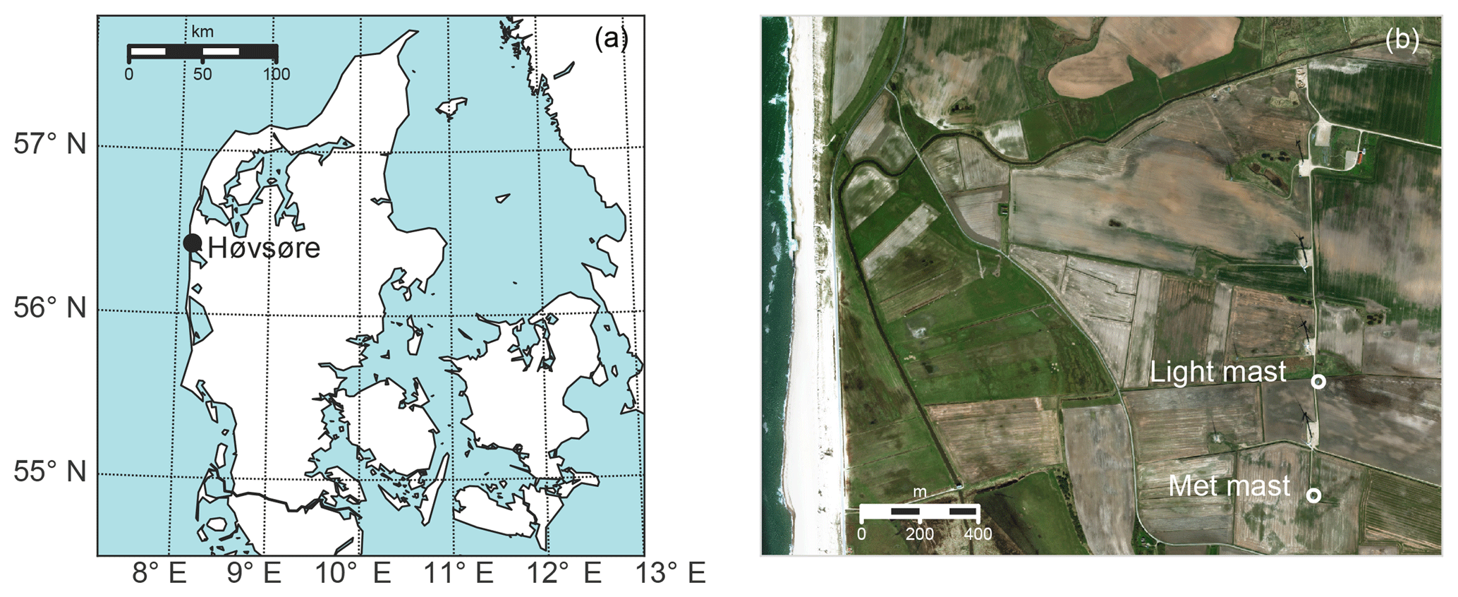
Figure 1(a) Map of Denmark showing the location of Høvsøre. (b) Overview of the Høvsøre test center showing the position of the met mast and the light mast with white circles.
We consider measurements only from the western sector, with 10 min mean wind direction between 225 and 315∘. This range of wind directions is chosen for two reasons: (i) to avoid measurements from the wakes of the wind turbines and flow distortion from the mast; and (ii) data from this sector correspond to coastal and offshore conditions.
2.1 Selection criteria of extreme events
For the selection of the extreme variance events the 10 min standard deviation of the wind speed measurements is compared to the extreme turbulence model in the IEC 61400-1 standard (IEC, 2005), wherein the horizontal turbulence standard deviation is given by
Here c is a constant of 2 m s−1, Iref is the reference turbulence intensity (TI) at 15 m s−1, Vave is the annual average wind speed at hub height, and Vhub is the 10 min mean wind speed at hub height, of which the variable σ1 is a linear function. For the “offshore” westerly directions considered at Høvsøre the long-term (10-year) mean of 10 min average wind speeds at a height of 100 m is U=10.4 m s−1, which corresponds well to class I turbines within the IEC 61400-1 framework with Vave=10 m s−1.
The IEC standard has three turbulence categories: A, B, and C, with A being the highest reference turbulence intensity and C the lowest. The corresponding reference TI for each class may be seen in Table 1. At Høvsøre, the (decade-long) average TI corresponding to the IEC reference wind speed, i.e., 10 min mean wind speeds of m s−1, is below 0.12. This indicates that the reference turbulence class C and Iref of 0.12 will equal or exceed in severity the actual conditions at the site. However, for the selection of events to analyze, a criterion corresponding to the IEC ETM with turbulence class B is used. This is done in order to limit the selection to a representative subset of the most extreme events, while also limiting computational demands. The selected events can be seen in Fig. 2 as blue dots that fall above the blue curve; i.e., these are events that have a high horizontal wind speed variance. The events are selected from measurements at a height of 100 m.
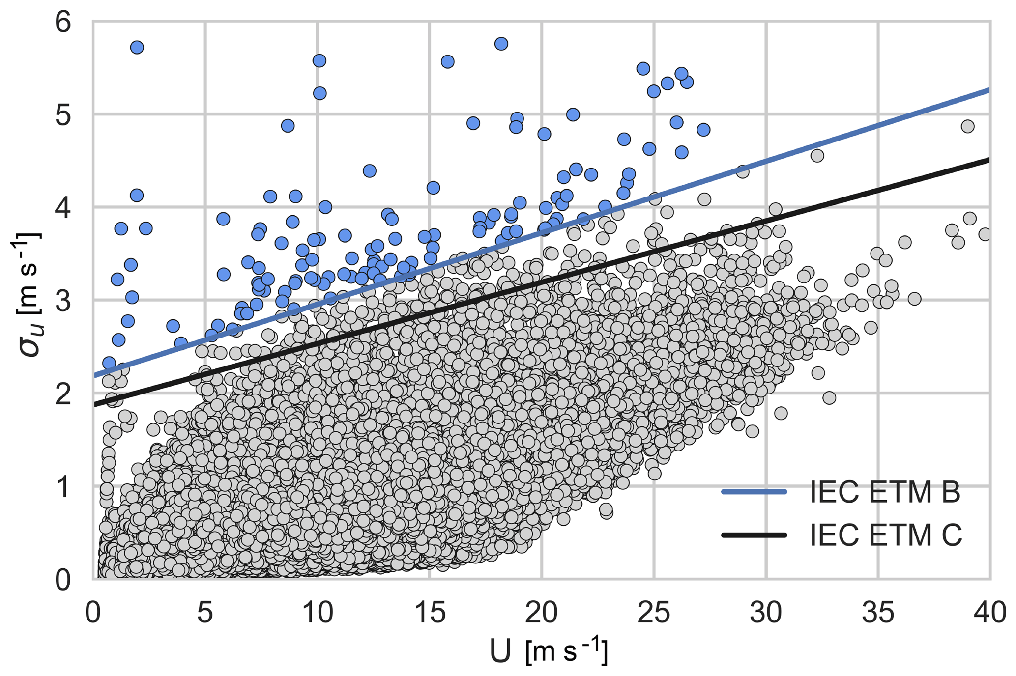
Figure 2The dots correspond to the 10 min standard deviation of the wind speed as a function of U at a height of 100 m over a 10-year period. The black and blue curves show the IEC extreme turbulence model for class C and class B, respectively. The selected events (blue dots) are σu values exceeding the extreme turbulence model class B.
Table 1The IEC turbulence classes and associated turbulence intensities.
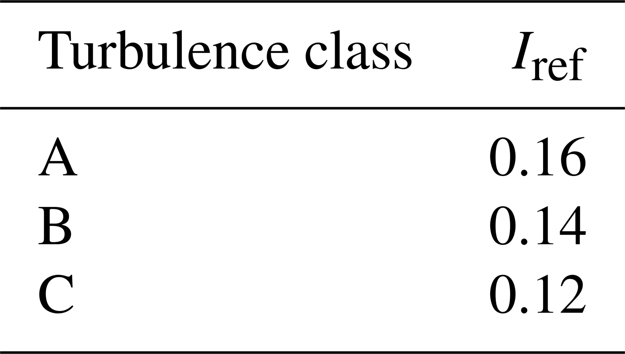
Figure 3 shows the horizontal wind speed at 100 m from the light mast and meteorological mast during six of the selected events. The events typically include a sudden rise in wind speed, which gives the main contribution to the high variance. Note that the sudden wind speed increase occurs approximately simultaneously at the two masts although they are ∼400 m apart (for mean wind direction roughly perpendicular to the line connecting the masts), indicating that the events are due to large coherent structures rather than extreme stationary turbulence.

Figure 3Comparison of horizontal wind speed measurements at the meteorological mast (green curve) and the light mast (blue curve). The measurement height is 100 m at both masts, which are separated by ≈ 400 m. The 10 min averaged wind direction is from the light mast.
The data set used for the data analysis and simulation is composed of the 10 Hz measurements from cup anemometers and wind vanes on the light mast in Høvsøre.
3.1 Estimation of 50-year joint extremes of turbulence and wind speed: IFORM analysis
The measurements shown earlier in Figs. 2 and 3 are raw (not processed or filtered), though it is common procedure to detrend data before estimating turbulence or associated return periods for a given turbulence level. Not all the extreme variance events are expected to be influenced by linear detrending, nor is such detrending necessarily appropriate for nonturbulent events; note, e.g., the event shown in Fig. 3c. Therefore we want to compare the 50-year return period of turbulence with the data detrended in two different ways: linear detrending and high-pass filtering. Detrending is performed by making a linear least-squares fit to the raw 10 min wind speed time series, with the linear component subsequently subtracted from the raw data.
The high-pass filtering is performed with a second-order Butterworth filter (Butterworth, 1930), whereby the magnitude of the frequency response function (the gain) is given by
where fc is the “cutoff” frequency. We perform the filtering using a cutoff frequency of 0.0017 Hz (1∕600 Hz) and also with a higher cutoff frequency of 0.0033 Hz (1∕300 Hz). The higher cutoff frequency chosen for the high-pass filtering corresponds to fluctuations with periods of 300 s (half of the period of the measurements). This choice of cutoff frequency ensures the removal of trends in the range 2.5–10 min (low-frequency transients) and is considered conservative enough to still include fluctuations associated with turbulent eddies.2
Here we use the inverse first-order reliability method (IFORM) to estimate the 50-year return period contour corresponding to the joint description of turbulence (σu) and 10 min mean wind speed (U). This method was developed by Winterstein et al. (1993) and provides a practical way to evaluate joint extreme environmental conditions at a site. The IFORM method is widely used in wind energy to predict extreme environmental conditions or long-term loading on wind turbines for ultimate strength analysis. More information on this method may be found in, e.g., Fitzwater et al. (2003), Saranyasoontorn and Manuel (2006), and Moon et al. (2014).
The first step in the IFORM analysis is to find the joint probability distribution f(U,σu). According to the IEC standard the 10 min mean wind speed is assumed to follow a Weibull distribution 3, and the “strength” (standard deviation) of turbulent stream-wise velocity component fluctuations (σu) is assumed to be lognormally distributed conditional on wind speed. In the standard, the mean of σu is expressed as a function of U,
and the standard deviation of σu is defined as
In Fig. 4, and are shown as functions of 10 min mean wind speed from Høvsøre unprocessed measurements at 100 m (grey dots) and the expressions from the IEC standard (blue lines) with Iref=0.12. The green lines show a third- and a second-order polynomial fit to the binned measurements of and , respectively (bins of 1 m s−1). The IEC expression for is higher than that from the measurements but has a similar slope for mean wind speeds above 15 m s−1. The difference is larger between the data and IEC expression for , for which the assumption of no mean wind speed dependency does not fit well to the data.
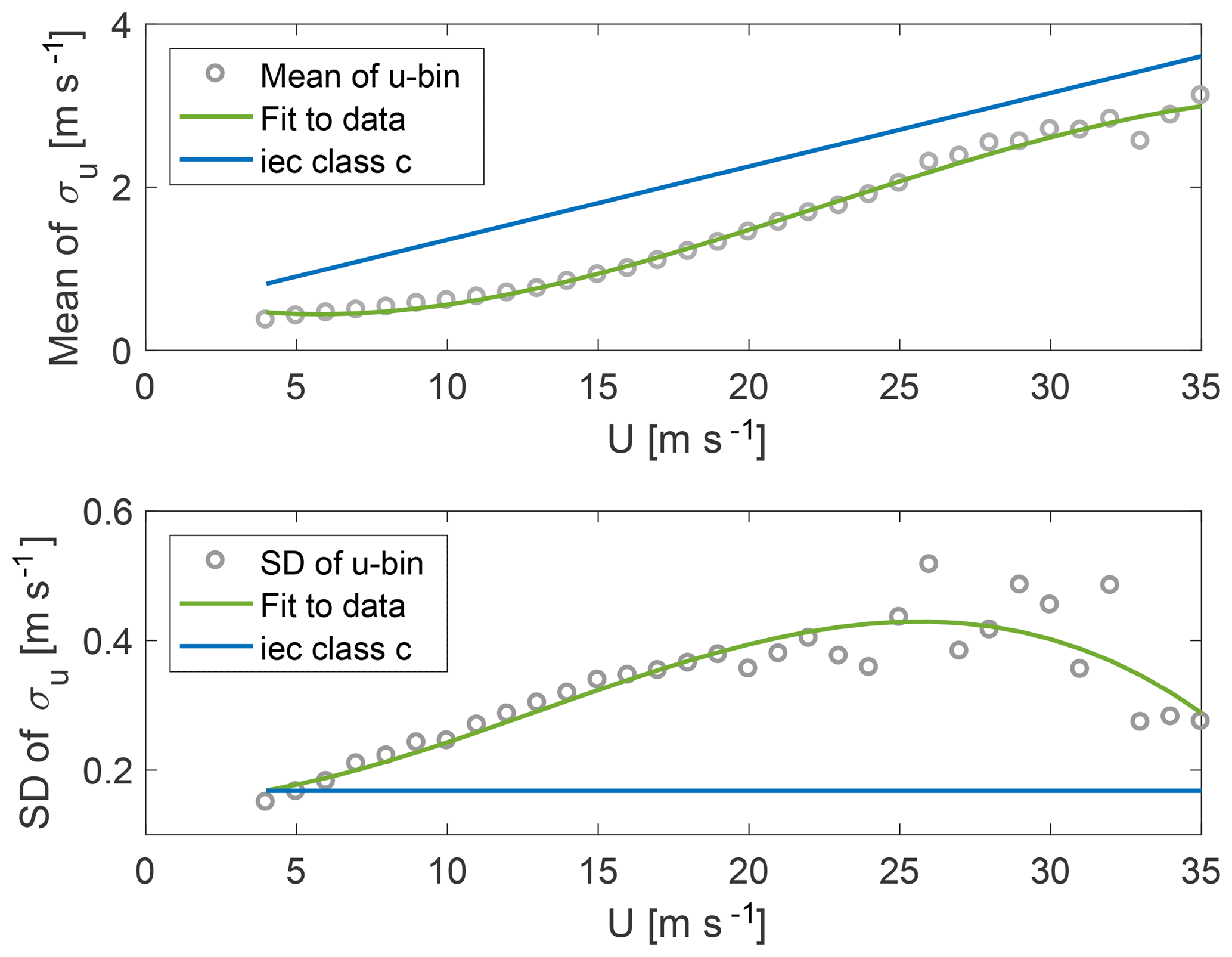
Figure 4The mean and standard deviation of σu as a function of wind speed at 100 m for raw data (not detrended or filtered). The blue curves show the IEC expressions, the grey dots show the measured values, and the green curves show a polynomial fit to the measurements.
The next step in the IFORM analysis is to obtain a utility “reliability index” β, which translates the desired return period Tr (here 50 years) into a normalized measure corresponding to the number of standard deviations of a standard Gaussian distribution:
Here Φ−1 is the inverse Gaussian cumulative distribution function (CDF), Tt is the duration of a turbulence measurement (here 10 min), and nm is the number of 10 min measurements corresponding to a 10-year period (which equals the time span of the data). Thus, the reliability index equals the radius of a circular contour in standard Gaussian space so that
where the standard normal variables u1 and u2 are derived from physical variables using an iso-probabilistic transformation, which takes correlations into account. We invoke the Rosenblatt transformation (Rosenblatt, 1952), which relies on the fact that a multivariate distribution may be expressed as a product of conditional distributions: . In this analysis, only two variables are considered, and the transformation may be performed in the following way:
where FU is the three-parameter Weibull CDF and is the conditional lognormal CDF.
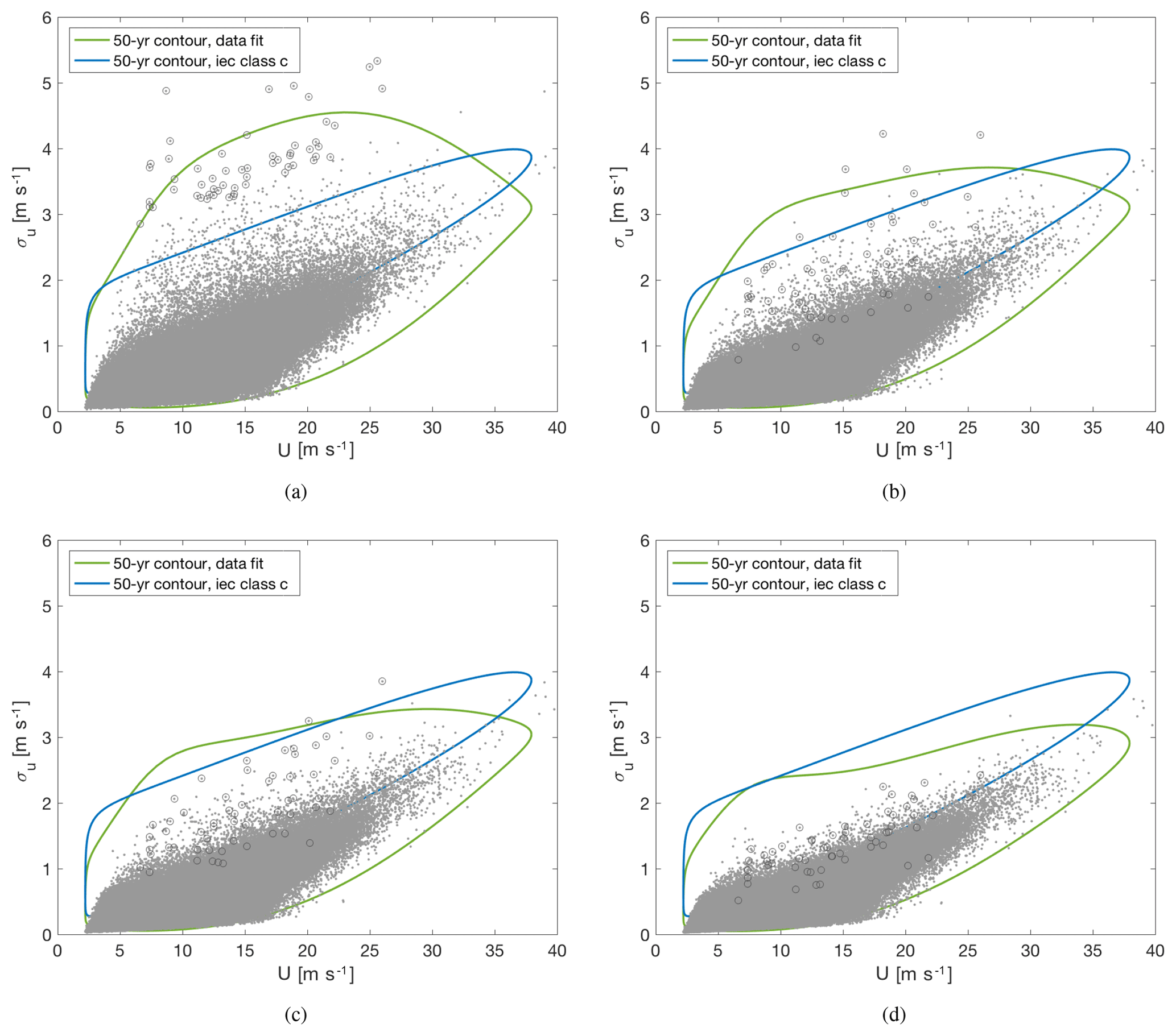
Figure 5The 50-year return period contours based on the measurements (green curves) and the IEC expressions (blue curves). The grey dots show the measurements. (a) Raw measurements. (b) Linearly detrended measurements. (c) High-pass-filtered measurements with a cutoff frequency of 1∕600 Hz. (d) High-pass-filtered measurements with a cutoff frequency of 1∕300 Hz. The dark grey circles indicate the extreme variance events.
Figure 5 shows the joint distribution of mean wind speed and turbulence4, with contours corresponding to the 50-year return period. The contours are calculated based on the measurements (green curves) and the IEC expressions (blue curves) of and , respectively. The parameters of the marginal distribution of the 10 min mean wind speed data were found with maximum likelihood estimation of the three-parameter Weibull distribution (scale parameter: 9.75 m s−1, shape parameter: 2.02, location parameter: 2.20). The parameters for the conditional lognormal distribution were estimated with the first and second moments, conditional on mean wind speed: and , both with the IEC expressions in Eqs. (3) and (4) and the third- and second-order polynomial fit to the binned data. It is seen when comparing Fig. 5a–d that the variance of σu is significantly reduced by the high-pass filtering. The 50-year return period contour estimated with the linearly detrended data (Fig. 5b) exceeds the one estimated with IEC turbulence class C in the whole operational wind speed range. This is because the linear detrending does not affect events like the one seen in Fig. 3c, and these events influence the estimate of the contour. Figure 5c shows the high-pass-filtered measurements with a cutoff frequency of 1∕600 Hz, and here it is seen how the estimated 50-year return period contour exceeds the IEC turbulence class C contour for wind speeds between 6 and 22 m s−1. In Fig. 5d, it is seen how the high-pass filtering with a cutoff frequency of 1∕300 Hz reduces the variance estimates to the extent that the 50-year contour obtained in this way gives turbulence levels lower than ETM IEC class C. These observed changes in turbulence levels indicate that the extreme variance events are not necessarily associated with linear trends. Some events are associated with wind speed fluctuations in a frequency range that may have a substantial impact on wind turbine loads. Therefore, we investigate this impact with constrained turbulence simulations incorporating the raw measurements that have not been detrended in any way.
3.2 Time series for simulation
The peak and the corresponding location of each event are identified in the following way: a moving average is subtracted from the wind speed signal and the maximum value of the differences identified:
where u is the horizontal wind speed signal and is the moving average over 60 s. The peaks are not necessarily the highest value of the signal, but rather the highest value within a sharp wind speed increase.
Applying the selection criteria described in Sect. 2.1 results in 99 identified events. Of these, 30 events are discarded as they include periods of missing measurements. A lower threshold of 4 m s−1 is put on upeak to exclude events mostly consisting of a linear trend or relatively insignificant peaks. Finally, events during which the corresponding directional data fluctuated below 180∘ are discarded, i.e., temporary directional data from the south, to exclude measurements from the wake of the nearby wind turbine. A remaining 44 events are chosen for load simulations. The measured time series including the extreme events are used to generate constrained turbulence simulations (explained in more detail in Sect. 4.4) of 600 s duration. The time series period is selected such that the sharp wind increase, or ramp, occurs approximately in the middle of the time series, i.e., approximately 300 s before and after the peak.
4.1 HAWC2 and the DTU 10 MW
Wind turbine response in the time domain is calculated with HAWC2 (Horizontal Axis Wind turbine simulation Code 2nd generation; Larsen and Hansen, 2015). HAWC2 is based on a multibody formulation for the structural part, whereby each body consists of Timoshenko beam elements. All the main components of a wind turbine are represented by these independent bodies and connected with different kinds of algebraic constraints. The aerodynamic forces are accounted for with blade element momentum theory (see, e.g., Hansen, 2013) with additional correction models: a tip correction model, a skewed inflow correction, and a dynamic inflow correction. HAWC2 additionally includes models that account for dynamic stall, wind shear effects on induction, tower-induced drag, and tower shadow.
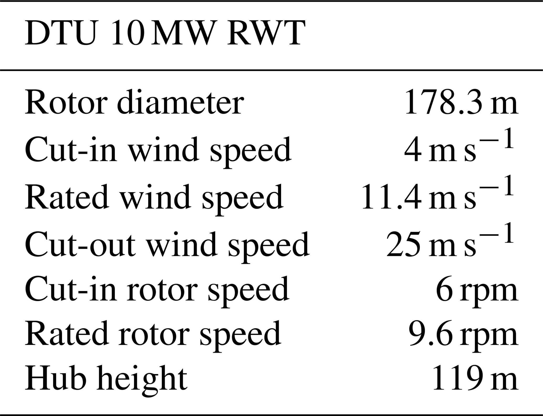
All the load simulations are performed using the DTU 10 MW reference wind turbine (RWT), which is a virtual wind turbine model based on state-of-the-art wind turbine design methodology. The main characteristics of the RWT may be seen in Table 2, and a more detailed description may be found in Bak et al. (2013). The controller used for the RWT is the Basic DTU Wind Energy controller (Hansen and Henriksen, 2013).
Table 2The main characteristics of the reference wind turbine.
4.2 Turbulence simulations in HAWC2
The Mann spectral turbulence model (Mann, 1994, 1998) is fully integrated into HAWC2, whereby a turbulence “box” may be generated for every wind turbine response simulation. The turbulence box is a three-dimensional grid that contains a wind velocity vector at each grid point. The turbulence boxes in this study all have grid points in the x, y, and z directions, respectively. The y–z plane is parallel to the rotor, and the distance between the grid points is typically defined so that the domain extent in the y and z directions becomes a few percent larger than the rotor diameter. The length of the x axis (Lx) is proportional to the mean wind speed at hub height, , where T is the simulation time. The turbulence box is transported with the average wind speed at hub height through the wind turbine rotor.
The Mann model is based on an isotropic von Kármán turbulence spectral tensor, which is distorted by vertical shear caused by surface friction. Assumptions of constant shear and neutral atmospheric conditions in the rapid distortion limit are used to linearize the Navier–Stokes equations, which may then be solved as simple linear differential equations. The solution results in a spectral tensor that may be used in a Fourier simulation to generate a random field with anisotropic turbulent flow. The Mann model contains three parameters, as described below.
-
Γ is an anisotropy parameter; when positive, , which are the variances of the u, v, and w components of the wind speed, respectively. When Γ=0, the generated turbulence is isotropic, .
-
αε2∕3 is the product of the Kolmogorov spectral constant and the rate of turbulent kinetic energy dissipation to the power of 2 ∕ 3. The Fourier amplitudes from the spectral tensor model are proportional to αε2∕3, and hence increasing αε2∕3 gives a proportional increase in the simulated turbulent variances but no change in the shape of the spectrum.
-
L is the length scale representative of the eddy size that contains the most energy.
The IEC-recommended values of the parameters are Γ=3.9 and L=29.4 m (for hub heights above 60 m), and αε2∕3 is set to a positive value to be scaled with . It has been shown in numerous studies that these parameters can change significantly, e.g., with turbulence level (Dimitrov et al., 2017; Kelly, 2018), atmospheric stability (Sathe et al., 2013; Chougule et al., 2017), and site conditions (Kelly, 2018; Chougule et al., 2015). As we do not want to investigate the effect of changing these parameters, all turbulence realizations are chosen to have the same parameters. In the present study, the anisotropy parameter is chosen according to the IEC standard, Γ=3.9. The turbulence length scale is chosen differently because the DTU 10 MW RWT is a relatively large wind turbine, and the turbulence length scale is expected to be of the same order of magnitude as the hub height (Kristensen and Frandsen, 1982). Here the length scale is estimated via
as derived by Kelly (2018). The final 200 s of simulation data, i.e., after the wind speed ramps, are used to estimate the length scale of turbulence and thus exclude the large coherent structure. Here σu from 100 m of height is used, along with dU∕dz estimated between z=160 m and z=60 m. Using Eq. (9) the length scale is found on average to be 〈L〉≈120 m over all events analyzed. The value chosen is therefore L=120 m.
4.3 Design load case 1.3
The DLC is simulated based on the setup described in Hansen et al. (2015), wherein mean wind speeds at hub height of 4–26 m s−1 in steps (bins) of 2 m s−1 are used, and each simulation has a duration of 600 s5. The Mann turbulence model is used to generate Gaussian turbulence boxes, with six different synthesized turbulence seeds per mean wind speed. The simulation time of the turbulence boxes is defined to be 700 s, the first 100 s of which are used for initialization of the wind turbine response simulation and are disregarded for the load analysis.
4.4 Constrained turbulence simulations
The aim here is to generate turbulence simulations resembling the measured wind field of the extreme variance events. This is done by constraining the synthesized turbulence fields. The constraining procedure involves modifying the time series to represent the most likely realization of a random Gaussian field that would satisfy the constraints using an algorithm described in Hoffman and Ribak (1991) and demonstrated with applications to wind energy in Nielsen et al. (2004) and Dimitrov and Natarajan (2017). For the constraining procedure we define three different random Gaussian fields as a function of location, :
-
the constrained field, f(r), which is the generated field of the procedure, modified to resemble the measurements;
-
the source field, , which here is a random realization of the Mann turbulence model; and
-
the residual field, which is the difference between the constrained field and the source field, .
The constraints are a set of M values at given locations, , which the constrained field is subject to, i.e., f(ri)=ci. At the constraint points, the residual field is given by , and for all other locations the values are conditional on the constraints in C. The conditional probability distribution of the residual field is denoted by the multivariate Gaussian distribution function
The conditional probability function of the field may be described as a shifted Gaussian around the conditional ensemble average 〈g(r)|C〉:
where 〈…〉 is the ensemble average, Ri(r)=〈f(r)Ci〉 represents the cross-correlations between the field and constraints, Rij=〈CiCj〉 represents the correlations between the constraints, and represents the values of the source field at the constraint locations.
A realization of the constrained field is generated by adding the conditional ensemble mean of the residual field to the source field:
Here the constraints consist of the u and v components of the wind velocity measurements from the light mast. The constraints are applied at three different heights: 79 m, 119 m (hub height), and 179 m, i.e., shifted up 19 m so the measurements at 100 m represent hub-height wind speed. The constraints are also applied at three different widths (along the y axis): 89.6 m (the middle of the turbulence box) ±70 m. This is done to ensure the coherent structure of the observed flow in the simulations. Every third measurement is applied at each width along the y axis, giving applied constraints at each y location with a 3.33 Hz frequency. This is done to reduce the number of applied constraints and thereby the computational time of the simulations.
In Fig. 6 two turbulence boxes with different random seeds are seen. The u component of the turbulent field is shown with a color scale on slices along the time axis. Figure 6a–b show the unconstrained turbulence boxes, and Fig. 6c–d show the same turbulence boxes with constraints corresponding to measurements from two different extreme variance events.
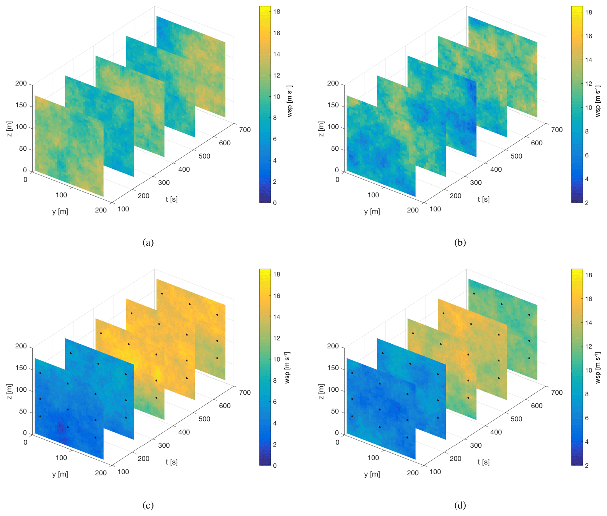
Figure 6Comparison between u velocity components from unconstrained turbulence simulations and from turbulence simulations with velocity jumps included using the constrained simulation. (a) Seed 1003 without constraints. (b) Seed 1005 without constraints. (c) Seed 1003 with constraints. (d) Seed 1005 with constraints. Constraint locations are shown with black dots.
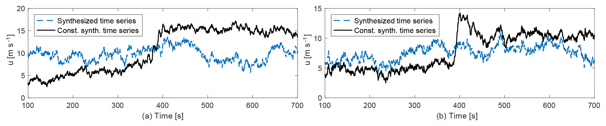
Figure 7Comparison of unconstrained and constrained stream-wise (u) velocity component in the middle of the turbulence box; y=89.6 m, z=119 m. (a) Seed 1003. (b) Seed 1005.
Figure 7 shows two examples of the u velocity time series at hub height with and without applied constraints for the same turbulence seeds as shown in Fig. 6.
For the purpose of load simulations, six different constrained turbulence seeds are generated from each extreme variance event time series. Although applying the constraints makes the turbulence boxes similar in general, there are differences in the parts of the boxes that are far from the constraint locations. As a result, there will be a seed-to-seed variation in loads simulated with constrained turbulence boxes, but they are much smaller than what is seen in the unconstrained case.
In this section we compare the design load levels of the two simulation sets: DLC 1.3 and the constrained simulations with the extreme variance. DLC 1.3 consists of 72 simulations (six seeds per 12 wind speed bins) and the constrained simulations consist of 264 simulations (six seeds per 44 extreme variance events).
5.1 Extreme loads
In Fig. 8 the standard deviation of the simulated hub-height u component wind speed is shown as a function of the mean hub-height u component wind speed. Each dot shows the standard deviation averaged over six turbulence seeds. As the variance is scaled to match the target for both DLC 1.3 and the constrained simulations, the scatter of the mean standard deviation over the six different seeds is small. The standard error of the mean standard deviation is in the range of 0.008–0.013 m s−1, and the standard error of the mean hub-height u component wind speed is equal to or less than 0.015 m s−1. The standard deviation from the constrained turbulence simulations (blue dots) is higher than that of DLC 1.3 with one exception. For this case, some variance was lost as a consequence of changing the time interval selection to span ±300 s around the wind speed peak, and data with a negative trend were cut off.
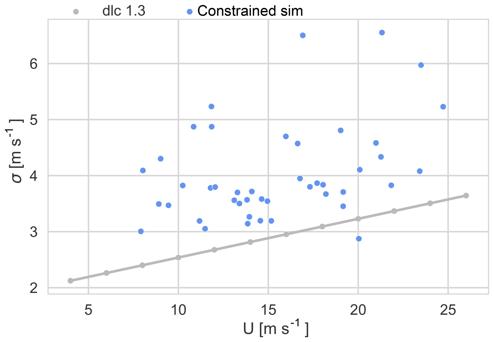
Figure 8The mean standard deviation of the u component of the simulated wind speed at hub height as a function of mean wind speed at hub height. DLC 1.3 (grey dots) and constrained simulations with extreme variance events (blue dots).
In Fig. 9 the characteristic extreme loads from DLC 1.3 and the constrained simulations are compared. The maximum–minimum load values of each 10 min HAWC2 simulation are binned according to wind speed with a bin width of 2 m s−1 and then averaged. For the comparison we omit the wind speed bin at 26 m s−1, as there are no observed events within that wind speed bin. The error bars show the standard deviation of the extreme loads of each wind speed bin. Both maxima and minima are shown for the tower-top moments, but for all other load components only the maximum moments are shown. It should be noted that the in-plane blade root flap moment maxima are negative due to the orientation of the blade coordinate system of the wind turbine model in HAWC2.
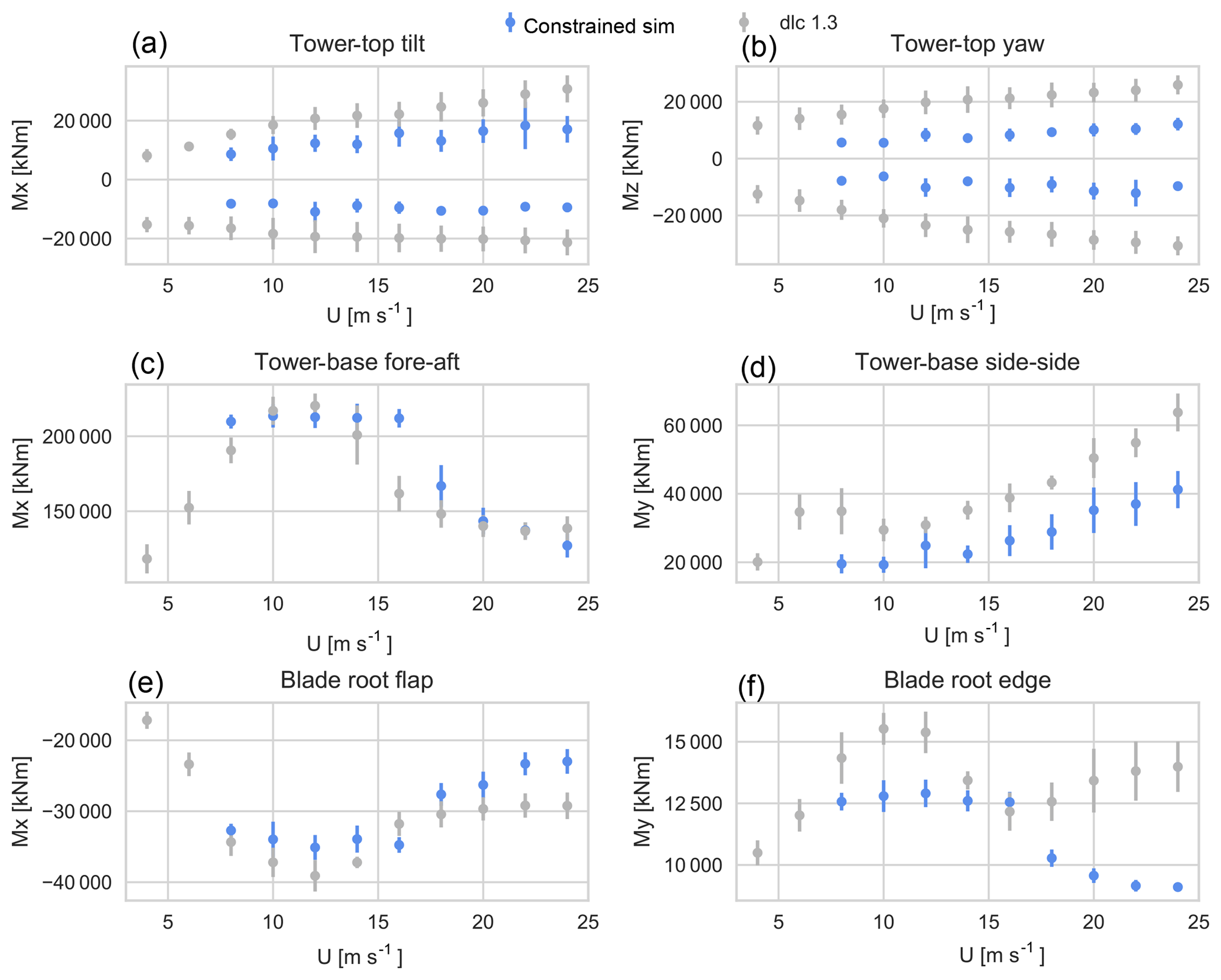
Figure 9The mean extreme moments from IEC DLC 1.3 (grey dots) and the mean extreme loads from the constrained simulations (blue dots).
Figure 9a and b show the extremes of the tower-top tilt and yaw moments, respectively. In the whole wind speed range the mean extreme moments for DLC 1.3 are between 6400 and 21 000 kNm larger than for the constrained simulations.
Figure 9c shows the mean extreme tower-base fore–aft moments. The overall highest mean extreme moment is from the DLC 1.3 simulation set; however, for the constrained turbulence simulations the loads are higher for wind speed bins at 8 m s−1 and between 14 and 20 m s−1. The largest difference is seen for wind speed bin 16 m s−1, wherein the mean extreme moment from the constrained simulation is 50 200 kNm larger than from the DLC 1.3.
Figure 9d shows the mean extreme tower-base side–side moments. In the whole wind speed range the mean extreme moments for the DLC 1.3 are between 6000 and 22 500 kNm larger than for the constrained simulations.
Figure 9e and f show the blade root flap and edge moments, respectively. In the whole wind speed range the mean extreme moments for the DLC 1.3 are between 800 and 6200 kNm larger than for the constrained simulations, with the exception of wind speed bin 16 m s−1, wherein the mean extreme moments from the constrained simulations are respectively 3000 and 400 kNm higher than the DLC 1.3.
The extreme tower-top tilt, yaw, and tower-base side–side moments show a general increase with wind speed. The extreme blade root flap and tower-base fore–aft moments peak around rated wind speed. For the extreme blade root edge moment it is seen that the loads peak around rated wind speed for both simulation sets, but the main difference is that after 16 m s−1 the DLC 1.3 loads and the scatter increase with wind speed.
Table 3The highest mean extreme moments for different load components
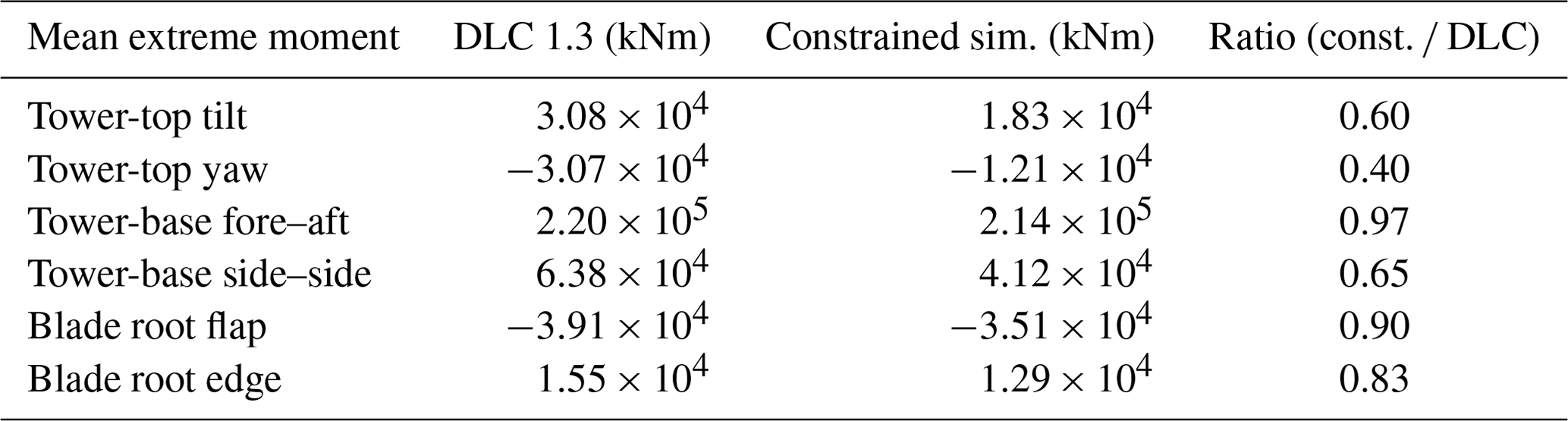
Table 3 lists the overall characteristic loads from each simulation set (the extremes seen in Fig. 9), together with their ratio. The difference between the overall extremes from the two simulation sets is largest for the tower-top yaw moment, wherein the extremes are lower from the constrained simulations. The overall extremes are of similar magnitude for the tower-base fore–aft moment and the blade root flap-wise moment.
5.2 Time series of turbine loads
In the following, examples of 10 min time series from DLC 1.3 and constrained simulation sets are shown side by side for comparison and a demonstration of the differences in the wind turbine response to different types of wind regime. A comparison is made for the tower-base fore–aft moment, wherein the characteristic extreme loads from the different simulation sets are of similar magnitude. We also consider and compare the tower-top tilt and yaw moments, which give the largest differences between the two simulation sets.
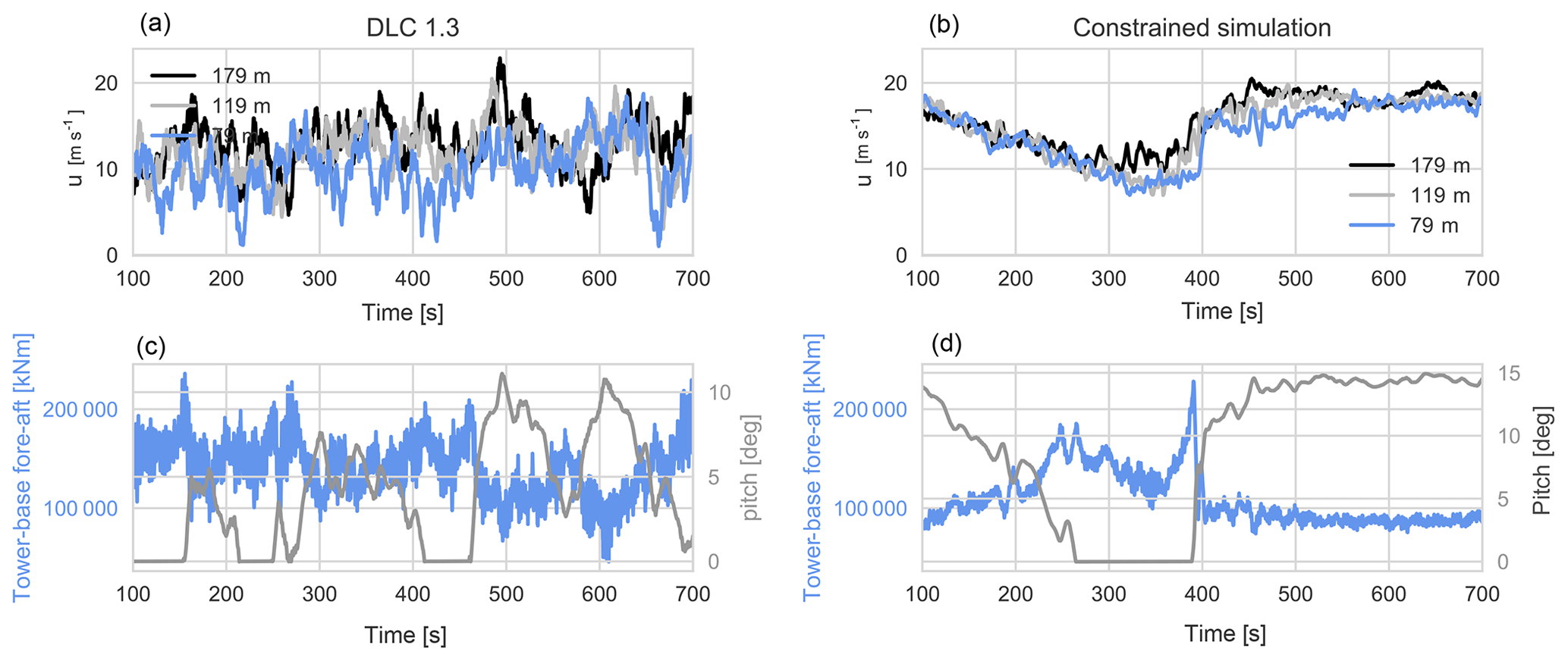
Figure 10Comparison of a DLC 1.3 time series (a, c) and a constrained simulation time series of an extreme event (b, d). (a, b) The u component wind speed. (c, d) Tower-base fore–aft moment (blue) and pitch angle (grey).
First, we compare two time series giving some of the highest extreme tower-base fore–aft moments from each simulation set. For DLC 1.3 in Fig. 10 the mean u component hub-height wind speed is U=12.0 m s−1, with a standard deviation of σu=2.7 m s−1, and the peak tower-base fore–aft moment is 236 000 kNm. For the constrained simulation, U=14.9 m s−1 and σu=3.5 m s−1. The peak tower-base fore–aft moment is 228 000 kNm. The peak tower-base fore–aft moments are of similar magnitude in the simulations, and in both cases this occurs when the pitch angle is zero degrees – right before the wind turbine blades begin to pitch. Also, at the time when the wind speed at hub height reaches rated wind speed, the wind speed at 179 m is above rated wind speed, leading to higher loading on the upper half of the rotor. From the turbulence simulations, the most noticeable difference in the wind turbine response is that in the constrained turbulence simulation the time of the peak tower-base fore–aft moment is very distinguishable at 390 s. While for the stationary turbulence the peak response occurs around 150 s, numerous times it reaches above 200 000 kNm during the simulation. Note that the axes in Fig. 10a and b are the same, as are the axes in Fig. 10c and d. It is seen that although the standard deviation of the wind speed is lower in the stationary turbulence simulation, the wind speed extremes are greater, with instantaneous wind speed reaching below 2 m s−1 and above 22 m s−1.
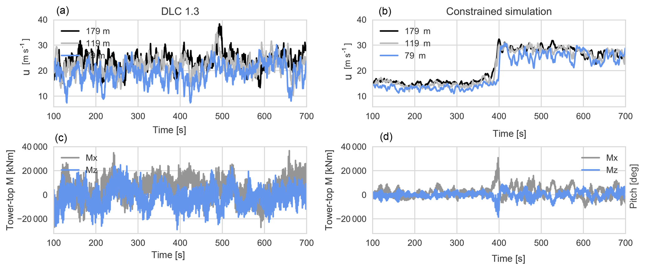
Figure 11Comparison of a DLC 1.3 time series (a, c) and a constrained simulation time series of an extreme event (b, d). (a, b) The u component wind speed. (c, d) Tower-top tilt (grey) and yaw (blue) moments.
In Fig. 11 we compare some of the most extreme tower-top moments from the two simulation sets. The stationary turbulence simulation in Fig. 11 has U=22 m s−1 and σu=3.4 m s−1, with a peak tower-top tilt moment of 36 601 kNm and a peak tower-top yaw moment of −28 900 kNm; in contrast, the constrained turbulence simulation has U=21.3 m s−1 and σu=6.6 m s−1, with a peak tower-top tilt moment of 30800 kNm and a peak tower-top yaw moment of −18 600 kNm. As in the previous example, the time of peak loads is very clearly identified in the constrained turbulence simulation, and the peak value is significantly higher than the response for the remainder of the simulation. For the stationary turbulence simulation, the tower-top yaw and tilt moments often reach high values throughout the simulation. Extreme tower-top moments tend to be observed when there is high shear across the rotor. In stationary turbulent flow the variation in wind speed across the rotor arises as turbulent eddies sweep by, hitting only part of the rotor, leading to high wind shear. The extreme tower-top loads from the constrained simulations are in connection with high vertical wind shear arising during the wind speed increase (ramp event).
In the load time series comparison, the general differences in the wind turbine response of the two simulation sets are visualized; for the constrained simulations the peak loads are distinguishable and occur because of the velocity increase associated with the ramp-like event. The discrepancies between the two simulation sets for the extreme tower-top loads indicate that the short-term wind field variability across the rotor is generally higher in the stationary turbulence simulation than for the constrained simulations. As shown in the time series comparison of Fig. 11, the short-term vertical wind shear can be high in connection with the extreme events, yet the tower-top tilt moment does not exceed that prescribed via DLC 1.3. When nonuniformity in the stationary turbulence fields occurs around rated wind speed, it can also lead to high extreme tower-base fore–aft moments that are connected to high thrust on the rotor. The extreme tower-base fore–aft moments from the constrained simulations are highest for mean wind speed bins between 8 and 16 m s−1. In this wind speed range, the wind speed is typically below rated wind speed at the beginning of the simulation and later increases beyond rated wind speed. When the wind speed starts to rise, it does so coherently across the rotor plane, resulting in high thrust and tower-base fore–aft moments, before the wind turbine controller starts to pitch the blades. The tower-base fore–aft moments for the extreme turbulence case (IEC DLC 1.3) were expected to be lower than those of the extreme variance events; however, this was generally true only (on average) for certain wind speed bins. The overall characteristic tower-base fore–aft moment of DLC 1.3 is 3 % higher than for the extreme events.
The load simulation results show that the extreme turbulence case DLC1.3 indeed covers the load envelope caused by extreme variance events. However, the differences seen in the time series and in the load behavior indicate that extreme variance observations as events are entirely different from situations with stationary, homogeneous turbulence. This questions the basis for the definition of the IEC extreme turbulence model (ETM), which is defined in terms of the statistics of the 10 min standard deviation of wind speed. As most observations of the selected extreme variance events include a short-term ramp event, it would perhaps be more relevant to compare these events with other extreme design load cases in the IEC standard, e.g., the extreme coherent gust with direction change, extreme wind shear, or the extreme operating gust. Since these are the absolute highest variance events observed at Høvsøre during a 10-year period, they would also appear in the site-specific definition of the ETM. Therefore, it may be necessary to exclude or reassign such events to the relevant load case type. The design and cost of a wind turbine may depend on how this consideration is done.
In the current study we generate Gaussian turbulence fields only, though it is known that atmospheric turbulence can exhibit some non-Gaussian character (e.g., Peinke et al., 2004; Wilczek and Friedrich, 2009; Morales et al., 2012). But the extent to which the non-Gaussian aspect impacts the response dynamics of wind turbines is the subject of ongoing debate. Studies have shown non-Gaussian wind fields to impact the loads on and output of wind energy converters; e.g., the torque fluctuations of a numerical wind turbine model (Mücke et al., 2011), the power and torque of a model wind turbine in a wind tunnel experiment (Schottler et al., 2017), and the power of a full-scale 2.5 MW wind turbine (Chamorro et al., 2015). However, a recent study based on large-eddy simulations of atmospheric turbulence shows that Gaussian and non-Gaussian turbulence, as input to wind turbine load simulations, results in insignificant differences (Berg et al., 2016). The conditions under which non-Gaussianity can significantly affect turbines (loads and power) still remain to be determined in ongoing research. The main focus of the current study is nonstationary ramp events and their impact on wind turbine loads, rather than a comparison of the Gaussian and non-Gaussian turbulence fields upon which the ramps are superposed. We use generated Gaussian turbulent fields as they are readily available, recommended by the IEC standard, and restrict the complexity of the study. Further, the loads are dominated by the ramp events and not by the turbulence.
It was seen in the IFORM analysis in Sect. 3.1 that the estimated 50-year return period contour of the linearly detrended data exceeded the 50-year return period contour of normal turbulence (corresponding to the ETM class C). This is consistent with the findings of Dimitrov et al. (2017), who performed a similar analysis of linearly detrended measurements from Høvsøre, though from the easterly (homogeneous farmland) sector. For the high-pass-filtered measurements, the turbulence level was reduced significantly, as was the estimated 50-year return period of turbulence. This is seen as the high-pass filtering effectively removes the variance of low-frequency fluctuations with timescales larger than 300 s, as the chosen cutoff frequency was 1∕300 Hz. This finding suggests that for the typical hub heights considered (z≈100 m) at a coastal site like Høvsøre, extreme variance events are not representative of homogeneous, stationary turbulence and can be filtered out by high-pass filtering. It should be kept in mind, though, that these events may be considered for extreme design load case purposes other than turbulence. In that case it is important not to use detrending of any kind on the measurements, as these extreme fluctuations will then not be identified and characterized correctly.
The main objective of this study is to investigate how extreme variance events influence wind turbine response and how it compares with DLC 1.3 of the IEC 61400-1 standard. The selected extreme events are measurements of the 10 min standard deviation of horizontal wind speed that exceed the values prescribed by the ETM and include a sudden velocity jump (ramp event, transients in the turbulent flow), which is the main cause of the high observed variance. The events were simulated with constrained turbulence simulations in which the measured time series were incorporated into turbulence boxes for load simulations in order to make a realistic representation of the events, including short-term ramps and coherent flow in the lateral direction as was seen in the comparison of measurements between the two masts in Fig. 2. The constraints force the turbulent flow of the simulations to be nonstationary and nonhomogeneous.
Load calculations of the simulated extreme events were made in HAWC2 and compared to load calculations with stationary homogeneous turbulence according to DLC 1.3. To summarize, we have found the following.
-
The extreme variance events are large coherent structures, observed simultaneously at two different masts with a 400 m (lateral) separation.
-
Most extreme variance events include a sharp wind speed increase (short-time ramp), which is the main source of the large observed variance.
-
High-pass filtering with a cutoff frequency of 1∕300 Hz removes most of the variance corresponding to these ramp-like events, to the extent that the estimated 50-year return period of the (remaining) turbulence level is lower than that of IEC ETM class C; linear detrending may remove some of the variance but is not necessarily adequate.
-
Compared with the DLC 1.3 of the IEC standard, the extreme loads are on average lower for the extreme variance events in the coastal and/or offshore climate and heights considered.
-
For 10 min mean wind speeds of 8–16 m s−1, the events typically begin below rated wind speed and increase beyond, leading to high thrust on the rotor; such events lead to high extreme tower-base fore–aft loads that can exceed the DLC 1.3 prescription of the IEC standard.
Future related work includes further analysis and characterization of extreme variance events. In particular, ongoing work involves extreme short-term shear associated with such events and directional change. Load simulations of the events may be compared with other extreme DLCs from the IEC standard.
The high-frequency measurements used for the data processing in Sect. 3 are stored at DTU Wind Energy in a SQL database that is not publicly accessible. The HAWC2 simulation outputs and wind speed inputs (turbulence boxes) are available as binary files upon request to Ásta Hannesdóttir (astah@dtu.dk).
The figure in this Appendix is equivalent to Fig. 4, but it shows the processed measurements.
Comparing the raw data in Fig. 4 to the linearly detrended data and high-pass-filtered data in Fig. A1, it is seen that the detrending and high-pass filtering slightly lowers the values of , while the reduction of is much greater, especially for the high-pass-filtered measurements.
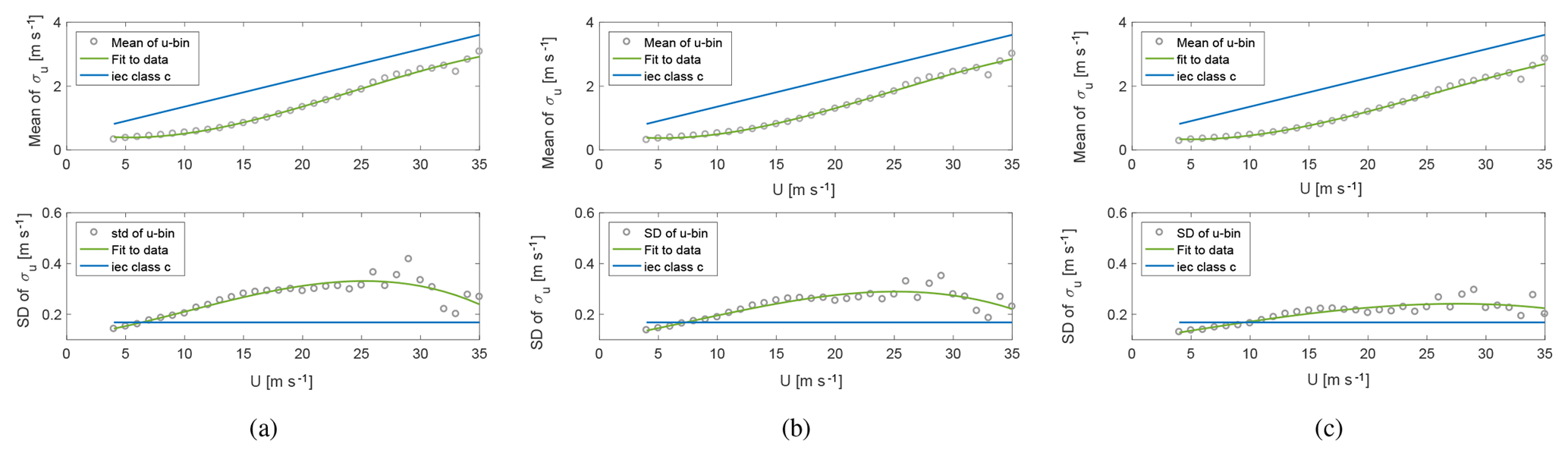
Figure B1 shows extreme moments as a function of the u component of the mean hub-height wind speed. Each dot is either a maximum or a minimum load value of each 10 min HAWC2 simulation for the tower top (top), tower base (middle), and blade root (bottom). The simulations based on a particular extreme variance event may be identified as a cluster of six dots, as they have been simulated with six different turbulence seeds. For DLC 1.3 a cluster of six dots may be seen, as the simulations are performed with six turbulence seeds per mean wind speed step. Figure 9 shows the values from Fig. B1, binned and averaged.
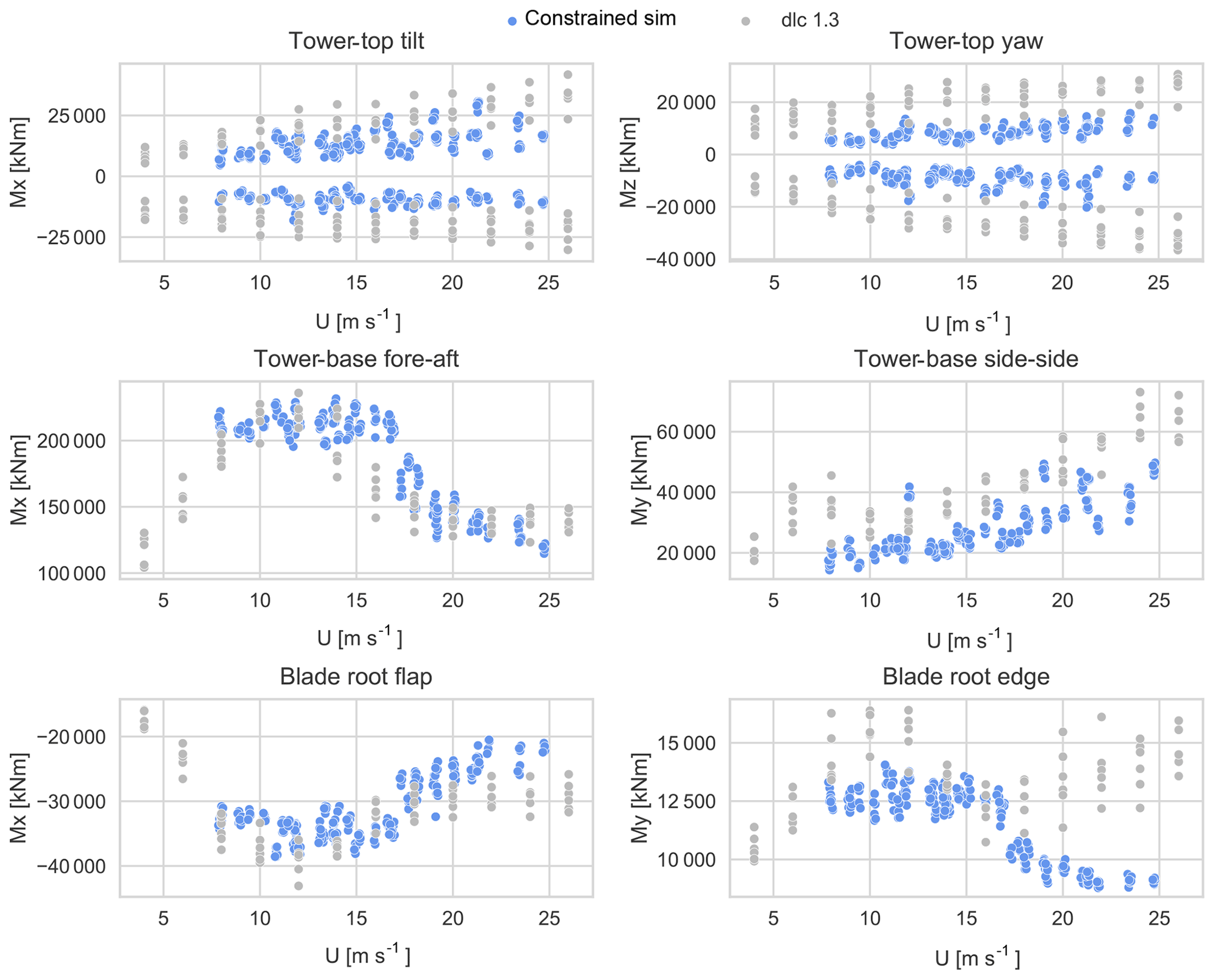
Figure B1The extreme moments from IEC DLC 1.3 (grey dots) and the extreme loads from the constrained simulations (blue dots).
ÁH performed the data analysis and simulations. ÁH made all figures. MK provided guidance and comments. ND developed the code that is used to perform constrained turbulence simulations. ÁH prepared the paper with contributions from the coauthors. This work is part of ÁH's PhD under the supervision of MK.
The authors declare that no competing interests are present in this work.
The authors would like to thank Anand Natarajan and Jakob Mann for constructive comments and discussion. Ásta Hannesdóttir would also like to acknowledge Jenni Rinker and David Verelst for HAWC2 assistance.
This paper was edited by Joachim Peinke and reviewed by three anonymous referees.
Bak, C., Zahle, F., Bitsche, R., Kim, T., Yde, A., Henriksen, L. C., Natarajan, A., and Hansen, M.: Description of the DTU 10 MW Reference Wind Turbine, Tech. rep., DTU Wind Energy, 2013. a, b, c
Berg, J., Natarajan, A., Mann, J., and G. Patton, E.: Gaussian vs non-Gaussian turbulence: Impact on wind turbine loads, Wind Energy, 19, 1975–1989, 2016. a
Butterworth, S.: On the Theory of Filter Amplifiers, Experimental Wireless and the Wireless Engineer, 7, 536–541, 1930. a
Chamorro, L. P., Lee, S.-J., Olsen, D., Milliren, C., Marr, J., Arndt, R., and Sotiropoulos, F.: Turbulence effects on a full-scale 2.5 MW horizontal-axis wind turbine under neutrally stratified conditions, Wind Energy, 18, 339–349, https://doi.org/10.1002/we.1700, 2015. a
Chougule, A., Mann, J., Segalini, A., and Dellwik, E.: Spectral tensor parameters for wind turbine load modeling from forested and agricultural landscapes, Wind Energy, 18, 469–481, https://doi.org/10.1002/we.1709, 2015. a
Chougule, A. S., Mann, J., Kelly, M., and Larsen, G. C.: Modeling Atmospheric Turbulence via Rapid Distortion Theory: Spectral Tensor of Velocity and Buoyancy, J. Atmos. Sci., 74, 949–974, https://doi.org/10.1175/JAS-D-16-0215.1, 2017. a
de Mare, M. T. and Mann, J.: On the Space-Time Structure of Sheared Turbulence, Bound.-Lay. Meteorol., 160, 453–474, https://doi.org/10.1007/s10546-016-0143-z, 2016. a
Dimitrov, N. and Natarajan, A.: Application of simulated lidar scanning patterns to constrained Gaussian turbulence fields, Wind Energy, 20, 79–95, https://doi.org/10.1002/we.1992, 2017. a
Dimitrov, N., Natarajan, A., and Mann, J.: Effects of normal and extreme turbulence spectral parameters on wind turbine loads, Renew. Energ., 101, 1180–1193, https://doi.org/10.1016/j.renene.2016.10.001, 2017. a, b, c, d
Fesquet, C., Drobinski, P., Barthlott, C., and Dubos, T.: Impact of terrain heterogeneity on near-surface turbulence structure, Atmos. Res., 94, 254–269, https://doi.org/10.1016/j.atmosres.2009.06.003, 2009. a
Fitzwater, L., Cornell, A., and Veers, P.: Using Environmental Contours to Predict Extreme Events on Wind Turbines, in: ASME proceedings, ASME 2003 Wind Energy Symposium, 244–258, 2003. a
Foster, R. C.: Why Rolls are Prevalent in the Hurricane Boundary Layer, J. Atmos. Sci., 62, 2647–2661, https://doi.org/10.1175/JAS3475.1, 2005. a
Foster, R. C., Vianey, F., Drobinski, P., and Carlotti, P.: Near-Surface Coherent Structures and The Vertical Momentum Flux in a Large-Eddy Simulation of the Neutrally-Stratified Boundary Layer, Bound.-Lay. Meteorol., 120, 229–255, https://doi.org/10.1007/s10546-006-9054-8, 2006. a
Hansen, M. H. and Henriksen, L. C.: Basic DTU Wind Energy controller, Tech. rep., DTU Wind Energy, Denmark, DTU-Wind-Energy-Report-E-0028, 2013. a
Hansen, M. H., Thomsen, K., Natarajan, A., and Barlas, A.: Design Load Basis for onshore turbines – Revision 00, Tech. rep., DTU Wind Energy, 2015. a, b
Hansen, M. O. L.: Aerodynamics of Wind Turbines, 2nd edn., Routledge, 2013. a
Hoffman, Y. and Ribak, E.: Constrained realizations of Gaussian fields - A simple algorithm, Astrophys. J., 380, L5–L8, https://doi.org/10.1086/186160, 1991. a
IEC: IEC 61400-1 Wind turbines - Part 1: Design requirements, 3rd edn., Standard, International Electrotechnical Commission, Geneva, Switserland, 2005. a, b
Kelly, M.: From standard wind measurements to spectral characterization: turbulence length scale and distribution, Wind Energ. Sci., 3, 533–543, https://doi.org/10.5194/wes-3-533-2018, 2018. a, b, c, d
Kristensen, L. and Frandsen, S. T.: Model for Power Spectra of the Blade of a Wind Turbine Measured from the Moving Frame of Reference, J. Wind Eng. Ind. Aerod., 10, 249–262, https://doi.org/10.1016/0167-6105(82)90067-8, 1982. a
Larsen, T. J. and Hansen, A. M.: How 2 HAWC2, the user's manual, Tech. rep., DTU Wind Energy, 2015. a, b
Mann, J.: The spatial structure of neutral atmospheric surface-layer turbulence, J. Fluid Mech., 273, 141–168, 1994. a, b
Mann, J.: Wind field simulation, Probabilist. Eng. Mech., 13, 269–282, 1998. a, b
Moon, J. S., Sahasakkul, W., Soni, M., and Manuel, L.: On the Use of Site Data to Define Extreme Turbulence Conditions for Wind Turbine Design, J. Sol. Energ.-T. ASME, 136, 044506, https://doi.org/10.1115/1.4028721, 2014. a
Morales, A., Wächter, M., and Peinke, J.: Characterization of wind turbulence by higher-order statistics, Wind Energy, 15, 391–406, https://doi.org/10.1002/we.478, 2012. a
Mücke, T., Kleinhans, D., and Peinke, J.: Atmospheric turbulence and its influence on the alternating loads on wind turbines, Wind Energy, 14, 301–316, https://doi.org/10.1002/we.422, 2011. a
Nielsen, M., Larsen, G., Mann, J., Ott, S., Hansen, K., and Pedersen, B.: Wind Simulation for Extreme and Fatigue Loads, Tech. rep., Risø National Laboratory, Roskilde, Denmark, 2004. a
Peinke, J., Barth, S., Böttcher, F., Heinemann, D., and Lange, B.: Turbulence, a challenging problem for wind energy, Physica A, 338, 187–193, https://doi.org/10.1016/j.physa.2004.02.040, 2004. a
Peña Diaz, A., Floors, R. R., Sathe, A., Gryning, S.-E., Wagner, R., Courtney, M., Larsén, X. G., Hahmann, A. N., and Hasager, C. B.: Ten Years of Boundary-Layer and Wind-Power Meteorology at Høvsøre, Denmark, Bound.-Lay. Meteorol., 158, 1–26, https://doi.org/10.1007/s10546-015-0079-8, 2016. a
Rosenblatt, M.: Remarks on a Multivariate Transformation, Ann. Math. Stat., 23, 470–472, https://doi.org/10.1214/aoms/1177729394, 1952. a
Saranyasoontorn, K. and Manuel, L.: Design Loads for Wind Turbines Using the Environmental Contour Method, J. Sol. Energ.-T. ASME, 128, 554–561, 2006. a
Sathe, A., Mann, J., Barlas, T. K., Bierbooms, W., and van Bussel, G.: Influence of atmospheric stability on wind turbine loads, Wind Energy, 16, 1013–1032, https://doi.org/10.1002/we.1528, 2013. a, b
Schottler, J., Reinke, N., Hölling, A., Whale, J., Peinke, J., and Hölling, M.: On the impact of non-Gaussian wind statistics on wind turbines – an experimental approach, Wind Energ. Sci., 2, 1–13, https://doi.org/10.5194/wes-2-1-2017, 2017. a
Vincent, C.: Mesoscale wind fluctuations over Danish waters, PhD thesis, DTU Wind Energy, 2010. a
Vincent, C., Hahmann, A., and Kelly, M.: Idealized Mesoscale Model Simulations of Open Cellular Convection Over the Sea, Bound.-Lay. Meteorol., 142, 103–121, https://doi.org/10.1007/s10546-011-9664-7, 2012. a
Wilczek, M. and Friedrich, R.: Dynamical origins for non-Gaussian vorticity distributions in turbulent flows, Phys. Rev. E, 80, 1–6, https://doi.org/10.1103/PhysRevE.80.016316, 2009. a
Winterstein, S. R., Ude, T. C., Cornell, C. A., Bjerager, P., and Haver, S.: Environmental parameters for extreme response: inverse FORM with omission factors, in: Proceedings of the 6th international conference on structural safety and reliability (ICOSSAR'93), 551–557, 1993. a
The light mast has aircraft warning lights on the top.
Fluctuations with a period of 300 s at 4–25 m s−1 (the operational wind speed range of a typical wind turbine) correspond to length scales of 1200–7500 m. Length scales in this range are significantly larger than turbulent length scales that have been estimated at the Høvsøre site (e.g., Sathe et al., 2013; Dimitrov et al., 2017; Kelly, 2018).
Here we use a three-parameter Weibull distribution. This is done because after filtering out measurements with errors and missing periods, the lowest mean wind speed is 2.2 m s−1. One could also use a weighted two-parameter Weibull distribution fit with increased weights in the tail to obtain the same result.
Note that some measurement points have been removed due to measurement errors; therefore, the points are fewer than in Fig. 2, which includes 10 min statistics from the whole measurement period.
In contrast with Hansen et al. (2015), here the simulations are performed without yaw misalignment.