A surrogate model approach for associating wind farm load variations with turbine failures

In order to ensure structural reliability, wind turbine design is typically based on the assumption of gradual degradation of material properties (fatigue loading). Nevertheless, the relation between the wake-induced load exposure of turbines and the reliability of their major components has not been sufficiently well defined and demonstrated. This study suggests a methodology that makes it possible to correlate loads with reliability of turbines in wind farms in a computationally efficient way by combining physical modeling with machine learning. It can be used for estimating the current health state of a turbine and enables a more precise prediction of the “load budget”, i.e., the effect of load-induced degradation and faults on the operating costs of wind farms. The suggested approach is demonstrated on an offshore wind farm for comparing performance, loads and lifetime estimations against recorded main bearing failures from maintenance reports. The validation of the estimated power against the 10 min supervisory control and data acquisition (SCADA) power signals shows that the surrogate model is able to capture the power performance relatively well with a 1.5 % average error in the prediction of the annual energy production (AEP). It is found that turbines positioned at the border of the wind farm with a higher expected AEP are estimated to experience earlier main bearing failures. However, a clear connection between the load estimations and failure observations could not be confirmed in this study. Finally, the analysis stresses that more failure data are required in future work to enable statistically significant associations of the observed main bearing lifetimes with load exposures across the wind farm and to validate and generalize the suggested approach and its associated findings.

1 Introduction

1.1 Motivation

For the past decades, wind energy has been one of the world’s fastest-growing sources of renewable energy, and it is expected to show a similar trend of growth in the future. The development of wind energy with increased wind turbine size and rated capacity has a significant influence on the operation and maintenance (O & M) costs (Gonzalez et al., 2016). Together with poor site accessibility as for offshore installations where wind turbines might be inaccessible for 4–5 months per year (Van Bussel and Zaaijer, 2001), failures are causing severe consequences in terms of downtime and maintenance costs (Bangalore and Patriksson, 2018). Therefore, optimizing the wind farm operation by improving performance and reliability in order to minimize the levelized cost of energy (LCoE) is gaining more and more importance. The O & M costs of wind turbines amount to around 25 % of the LCoE for onshore wind turbines and 35 % for offshore wind turbines (Dinwoodie et al., 2012). For reducing the O & M costs, monitoring and predicting the condition of the turbine's components in terms of operational health, material degradation and remaining lifetime plays an important role. Improving the detection rate of a monitoring system for blades, drive train, tower and grout from 60 % to 99 % for instance results in an increase of lifetime levelized savings by 32 % (May et al., 2015).

Most current wind turbine maintenance strategies are time-based and assume a reliability degradation dependent on the system age (Reder and Melero, 2018). Throughout the lifetime of a turbine, its failure rate is assumed to follow a Weibull distribution with a higher failure frequency in the first years of operation, followed by a longer period of a lower constant failure rate. Towards the end of life, an increasing failure rate can be observed again due to wear and damage accumulation caused by fatigue loading (Mudholkar and Srivastava, 1993; Hahn et al., 2007).

However, the relation between the load exposure of turbines in a wind farm and their component reliability has not been sufficiently well defined and demonstrated. Characterizing this relation would enable to assess the current health state of a turbine and help to better understand the effect of load-induced degradation and faults on the operating costs of wind farms. Especially for offshore wind farms where failures can lead to high downtime, this plays an important role for reducing the LCoE.

1.2 Objective

The objective of the present paper is two-fold:

• Firstly, the aim is to suggest a methodology that makes it possible to investigate the correlation between loads and component reliability of turbines in wind farms, by combining data (10 min averages from a supervisory control and data acquisition, SCADA, system) and physical modeling (HAWC2 aeroelastic load simulations) with machine learning.

• Secondly, the suggested approach is demonstrated on a case study to investigate whether the loading conditions can be clearly associated with the observed reliability of the main bearing.

1.3 Background and related work

Information about the turbine reliability can be derived either by modeling structural reliability parameters (e.g., failure frequency, likelihood of observing failure over a reference period) or by using collected data from inspection and maintenance reports (e.g., observed failure rates, observed time to failure). Opposed to the assumption that turbine reliability only decreases with operational time, several studies have demonstrated the effect of meteorological conditions on the turbine reliability, such as Reder and Melero (2016) and Tavner et al. (2006). Also example studies of the influence of wake effects on the turbine reliability can be seen in Kim et al. (2012) and Huang and Chiang (2006). Previous work aimed at defining a relationship between fatigue and extreme loading conditions on a turbine and its reliability can be found in Colone et al. (2018) and Scott et al. (2012). Colone et al. (2018) modeled the impact of turbulence induced loads on the fatigue reliability of offshore wind turbine monopiles. In Scott et al. (2012) the damage effect of extreme and transient loads on the drivetrain reliability is estimated. However, these studies focus on modeling the reliability, rather than investigating observed failure rates from measurement data. Therefore, the present paper aims at suggesting a methodology for modeling various wake-induced loads, performance and estimated lifetime, and comparing it against measured failure rates and times to failure. The suggested approach can be used for modeling various performance and load variables under different operating conditions.

Modeling wake-induced loads in wind farms is a crucial step for fatigue load assessments both in the design process and during the operational phase of a wind farm where load measurements are costly and therefore rarely conducted. Carrying out aeroelastic simulations each time a load assessment is required is impractical. Therefore, various methods have been developed to reduce the number of computations required. A popular approach is the use of so-called surrogate models which are reduced-order models that are trained on a limited number of aeroelastic simulations. Once the surrogate model has been trained, multiple site-specific load assessments at arbitrary sites can be obtained at a low computational cost and without the need of new aeroelastic simulations. Examples are Toft et al. (2016) and Müller et al. (2017), who propose a methodology based on response surface (RS) for site-specific load estimations. Teixeira et al. (2017) demonstrate the use of kriging surfaces for fatigue load estimations of offshore wind turbines.

These approaches focus solely on one surrogate model and use a relatively small variable space. In Dimitrov et al. (2018) the surrogate model framework is expanded with the motivation to fully characterize the wind field conditions, as well as to enable comparing different surrogate models within the framework. Based on this framework, a benchmark of different surrogate models in Schröder et al. (2018) has shown that an artificial neural network (ANN)-based surrogate model outperforms other methods using polynomial chaos expansion and RS in terms of model accuracy, computational time as well as convergence stability.

The abovementioned approaches are only applicable for estimations on single turbines. In Dimitrov (2019) the surrogate modeling framework is extended in order to estimate wake-induced loads for a wind farm with arbitrary layout. In this approach the number of simulations required for modeling different wake conditions is reduced by parametrizing the wake effects. This method has been demonstrated in a case study on the Horns Rev I wind farm (Galinos et al., 2016) and further validated against measurement data in Dimitrov and Natarajan (2019). In the present study, the abovementioned wind farm surrogate modeling framework is expanded for estimating further performance and lifetime parameters under additional operating condition, and its predictions are compared against observed failures.

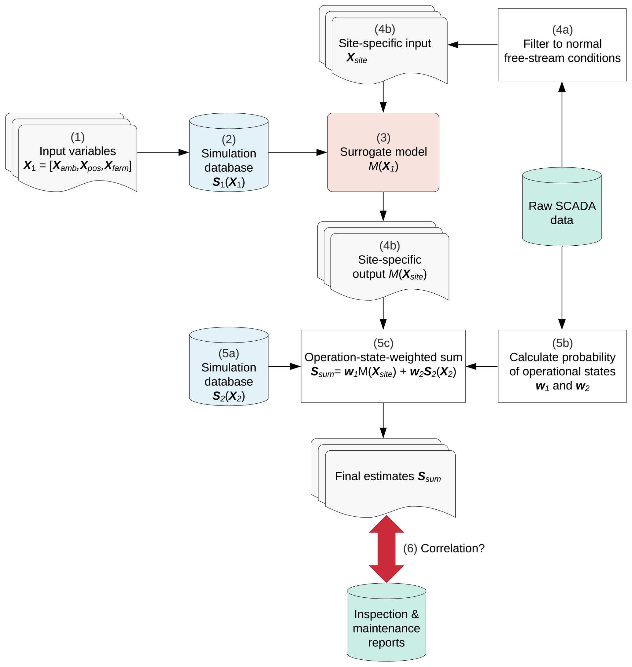
Figure 1 Methodology for estimating performance, loading condition and lifetime characteristics within a wind farm.

2 Methodology

The suggested methodology for comparing wake-induced loads against the component reliability of turbines is illustrated in Fig. 1. It can be used to estimate various performance, loading and lifetime characteristics of a wind farm. The approach can be applied to any wind farm with arbitrary layout and turbine type as long as data recorded from the SCADA system are available together with observed failure events, e.g., from inspection and maintenance reports. The framework can be split into six main steps which are more thoroughly described in the following sections:

1. define variable input space and create samples X₁ from predefined distributions and boundaries;

2. create high-fidelity simulation database for normal operation S₁(X₁), to be used as training inputs for a surrogate model;

3. train a surrogate model M(X) (an ANN) mapping undisturbed environmental conditions to load and power outputs;

4. obtain site-specific load and power estimations under normal operating conditions, M(X_site), by sampling the surrogate model over the joint distribution of site-specific environmental conditions X_site;

   • a.

     establish a site-specific joint probability distribution of undisturbed wind conditions by analyzing measured data;

   • b.

     carry out a Monte Carlo (MC) simulation with the surrogate model, drawing samples X_site from the site-specific joint distribution;

5. add other operational conditions (e.g., transients such as start-ups and shutdowns);

   • a.

     simulate scenarios with the selected (transient) operating conditions S₂(X₂);

   • b.

     analyze SCADA data and fault and event logs to establish the annual frequency of the events;

   • c.

     weight estimates according to the probabilities of the operational states w₁ and w₂ obtained from data;

6. compute a summary statistic S_sum to be considered as a proxy for component reliability and compare estimates against observed failure events.

2.1 Define variable input space and sample from predefined distributions

Selecting the variable input space is a crucial step in the creation of the simulation database. The performance and mechanical load variations of turbines within a wind farm mainly depend on the wake-induced turbulence. In this analysis, the wake-induced turbulence is characterized by variables that can be grouped into ambient conditions X_amb, turbine position X_pos and wake-induced effects X_farm based on the study by Dimitrov (2019):

• X_amb=[u, σ_U, α, H_s, T_p, Δ] (mean wind speed, turbulence, wind shear, significant wave height, wave peak period and wind‐wave misalignment);

• X_pos=[Z_w] (water depth);

• X_farm=[R_D, γ, N_rows] (row spacing, wake incidence angle and number of disturbing turbines).

The environmental variables from X_amb and X_pos include the most relevant factors that affect mechanical loads on both the nacelle and the foundation. The variables from X_farm intend to describe the relative position of the wake source(s) with respect to the disturbed turbine such that the model is generalized for arbitrary wind farm layouts. The choice of the three wake-induced variables of X_farm is explained more in detail in Dimitrov (2019).

To make sure that the model is able to cover a wide range of conditions, the distributions and boundary functions of each variable have to be defined accordingly. Since some of the ambient variables are conditional on each other, the variable space is generated by sampling from their joint probability distribution using a Rosenblatt transformation (Rosenblatt, 1952) that takes into account the predefined distributions and bounding functions (Dimitrov, 2019).

It should be noted that the variable space should be defined specifically for each use case. For instance, if only nacelle load estimates are of interest, the variables for wave-induced loads (H_s, T_p, Δ) can be neglected since they most likely will not effect the final estimates.

2.2 Create aeroelastic simulation database

The set of sampled input variables which can be represented as X=[X_amb, X_pos, X_farm] is then used for simulating the desired output variables S(X) (see Fig. 2). For running aeroelastic time series simulations a wind flow model as well as a wake model that allows the superposition of multiple wake sources N_rows for modeling wake-induced effects is required. Furthermore, a structural model, aerodynamic model and the controller of the turbine need to be included in order to model the structural response. In case this approach is applied to offshore turbines, also a hydrodynamic model and soil model (or alternatively a simplified apparent fixity model) are necessary for including the effects of hydrodynamic and soil forces.

Figure 2 Process of aero-servo-hydro-elastic simulations using sampled input variables.

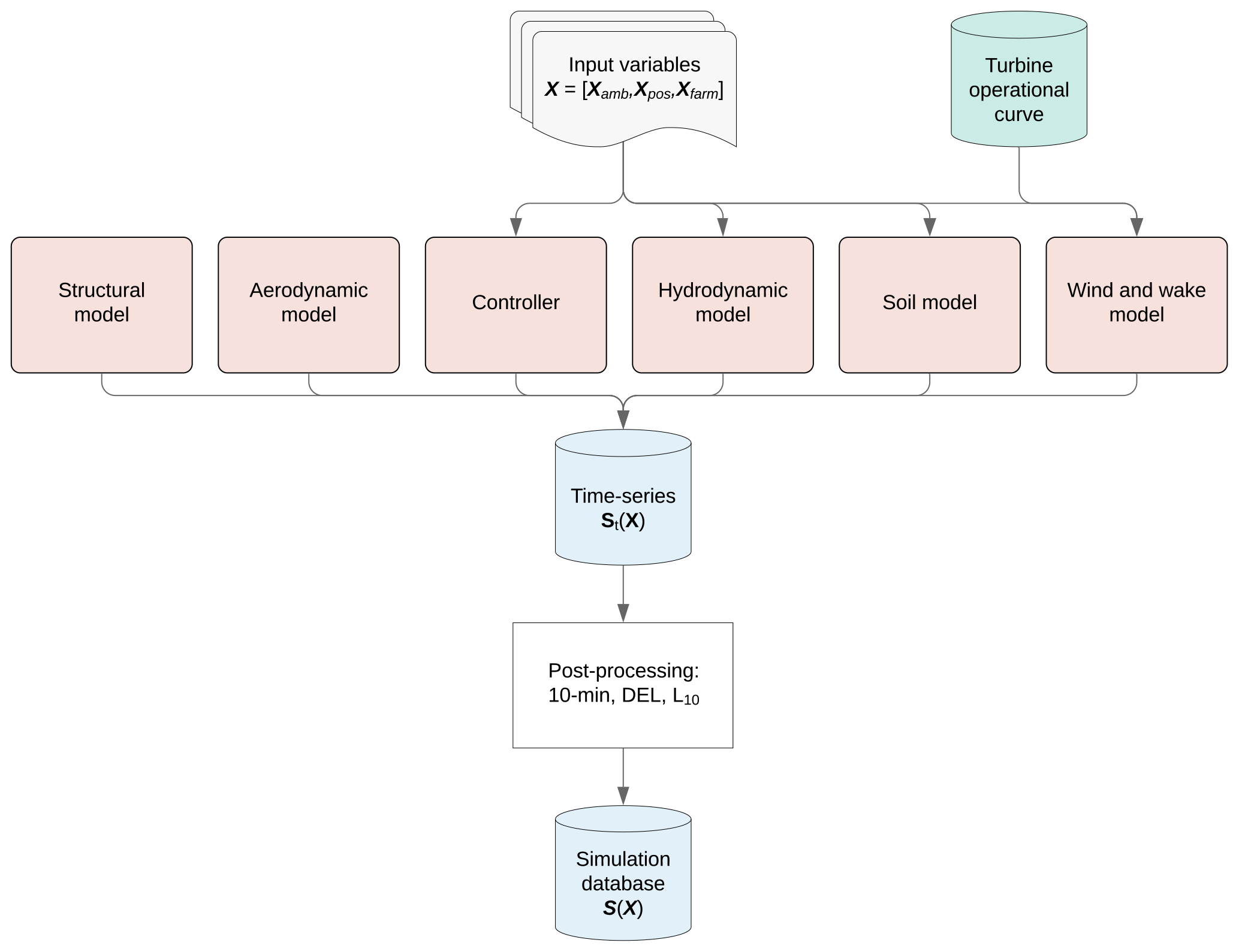
Subsequently, the time series simulations S_t(X) are post-processed in order to obtain 10 min statistics, lifetime indicators and damage-equivalent fatigue loads (DELs) for assessing performance, lifetime or fatigue. By applying the Palmgren–Miner's rule the lifetime DEL can be formulated for a given Wöhler exponent m using the following equation:

$$\begin{array}{}\text{(1)}& \mathrm{DEL}={\left({\displaystyle \frac{\underset{u}{\int }\underset{\mathit{\theta }}{\int }{R}_{\mathrm{eq}}(u,\mathit{\theta }{)}^m{n}_{\mathrm{eq}}p(u,\mathit{\theta })\mathrm{d}u\mathrm{d}\mathit{\theta }}{n_{\mathrm{eq},\mathrm{L}}}}\right)}^{\mathrm{1}/m},\end{array}$$

with the 1 Hz equivalent fatigue load R_eq that is simulated, e.g., for 600 s corresponding to n_eq=1 Hz ⋅ 600 s = 600 equivalent cycles, the joint probability p(u, θ) of the wind speed u and wind direction θ and the number of equivalent cycles n_eq,L corresponding to operation over the intended lifetime of the wind farm.

For assessing the component reliability of a main bearing, the fatigue life indicator L₁₀ for which 10 % of the bearings would not survive (Calderon, 2015) can be calculated:

$$\begin{array}{}\text{(2)}& L_{\mathrm{10}}={\displaystyle \frac{a_{\mathrm{1}}{a}_{\mathrm{2}}{a}_{\mathrm{3}}{\mathrm{10}}^{\mathrm{6}}}{\mathrm{60}n}}{\left({\displaystyle \frac{C}{P_{\mathrm{d}}}}\right)}^p\left[\mathrm{years}\right],\end{array}$$

where n is the rotational speed, a_i, i=1, 2, 3 are life correction coefficients, C is the dynamic bearing rating and $p=\mathrm{10}/\mathrm{3}$ is the life exponent for roller bearings. A high value indicates a longer main bearing lifetime. The dynamic equivalent force P_d is defined as a hypothetical force resulting in the same lifetime as if acting on the bearing center as pure radial load (in case of radial bearing) or pure axial load (in case of thrust bearing) (NTN, 2009). It can be calculated using the radial force F_r and the axial force F_a as follows:

$$\begin{array}{}\text{(3)}& P_{\mathrm{d}}=b_x{F}_{\mathrm{r}}+b_y{F}_{\mathrm{a}},\end{array}$$

with calculation factors b_x and b_y that depend on the specific roller bearing type; i.e., if $\frac{F_{\mathrm{a}}}{F_{\mathrm{r}}}\le \mathrm{0.27}$, then b_x=1 and b_y=2.5. Otherwise if $\frac{F_{\mathrm{a}}}{F_{\mathrm{r}}}>\mathrm{0.27}$, then b_x=0.67 and b_y=3.7.

2.3 Train surrogate model

Once the simulation database is created, the surrogate model can be trained using the set of input variables X and set of target variables S(X) as shown in Fig. 3. As mentioned before, the selection of which variables should be included in the target set S(X) depends on the intention of the specific use case.

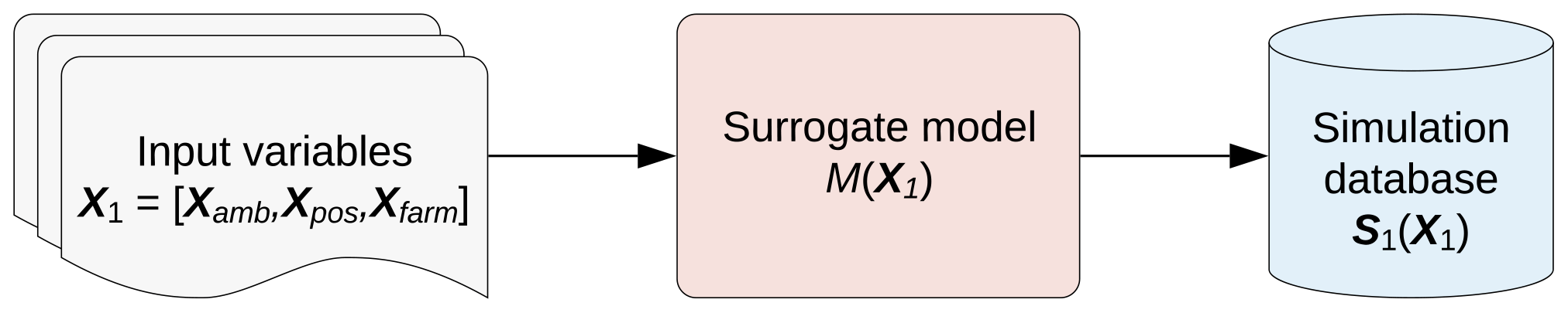
Figure 3 Schematic illustration of site-specific wind farm load estimation using surrogate model.

The transfer function for mapping the input variables to the targets can be any type of regression model. However, this study suggests using feed-forward ANNs, since they were found to be the most suitable method for the task of site-specific load estimations in terms of prediction time, accuracy and convergence robustness with smaller training samples (Schröder et al., 2018).

Feed-forward ANNs (Goodfellow et al., 2016) consist of multiple fully connected layers. In each layer the input x is transformed linearly to $\mathit{z}=\mathbf{W}\mathit{x}+\mathit{b}$ with weight matrix W and bias b. After the result is passed through a non-linear activation function σ(z), it will serve as input to the next layer ${\mathit{x}}^{[i+\mathrm{1}]}=\mathit{\sigma }\left({\mathit{z}}^{\left[i\right]}\right)=\mathit{\sigma }({\mathbf{W}}^{\left[i\right]}{\mathit{x}}^{\left[i\right]}+{\mathit{b}}^{\left[i\right]})$. When training an ANN, the weight parameters W and bias parameters b can be estimated by minimizing the cost function J(W, b). The cost function is a measure of the difference between the model prediction g(W, b, x) and the observed output y. When using a least-squares approach the cost function can be calculated as shown in Fig. 4, where N_e is the number of training samples.

$$\begin{array}{}\text{(4)}& J(\mathbf{W},\mathit{b})=\sum _{i=\mathrm{1}}^{N_{\mathrm{e}}}{\left(y_i-g\left(\mathbf{W},\mathit{b},{\mathit{x}}_i\right)\right)}^{\mathrm{2}}\end{array}$$

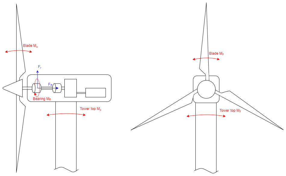
Figure 4 Wind turbine schematic including loads considered in this study: blade-root bending moments M_x and M_y, tower-top bending moments M_x and M_y, bearing torsional moment M_z, main bearing axial force F_a and main bearing radial force F_r.

2.4 Site-specific estimations using surrogate model

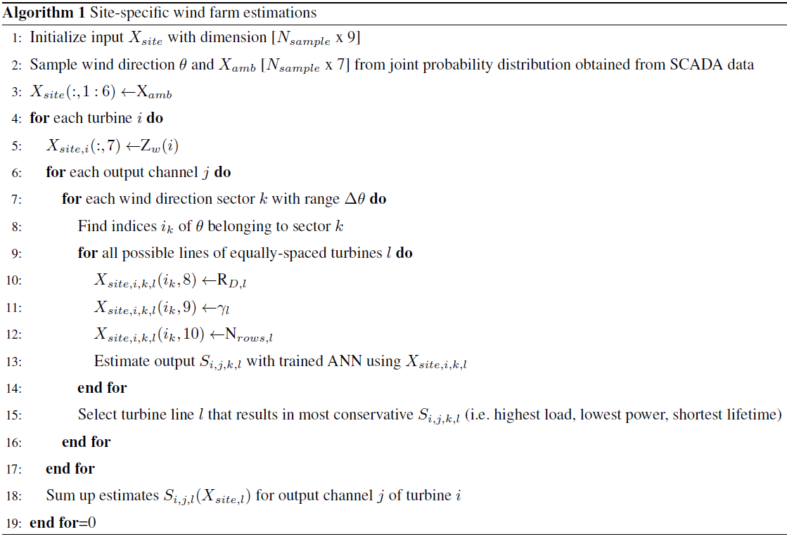
In order to deploy the trained surrogate model to give estimations for the desired offshore wind farm, a new input data set has to be generated that includes the site-specific ambient environmental conditions, as well as farm-related parameters for the specific wind farm. Similarly as in Sect. 2.1, the ambient input variables X_amb are sampled with a Monte Carlo simulation using Rosenblatt transformation in order to construct the site-specific joint probability distributions with the wind direction θ being the first independent variable. The distributions of these ambient conditions can be obtained from any available measured or modeled source, such as SCADA data or a meteorological mast. Since the input variables X_pos and X_farm on the other hand depend on the turbine position within the wind farm, they have to be generated for each turbine separately. Regarding the wake-related input X_farm, the row spacing R_D, wake incident angle γ and number of upstream turbines N_rows have to be collected for each wind direction sector separately. The trained ANN is then applied using these input variables X_amb, X_pos and X_farm for estimating the output S(X_site). In case there are several lines of turbine rows upstream, the output is estimated for each equally spaced turbine line and the most conservative estimate is selected. Algorithm 1 shows the implementation steps required for the abovementioned procedure. For a more detailed explanation of this approach including an implemented example case, see Dimitrov (2019).

The estimations from the ANN are then simply summed up for each turbine. A probability weighting of the samples is not necessary since they are already generated taking into account the probability distributions of the input space. The annual energy production (AEP) of each turbine can be calculated using Eq. (5) with the number of Monte Carlo samples N_sim, estimated electrical power $\widehat{P_i}$ and the number of operating hours per year N_hours,y. The DEL values can be summed up according to Eq. (6). Note that before the summation, the estimations ${\widehat{L}}_i$ need to be inverted to 1 Hz fatigue range sums $L_{\mathrm{inv},i}=\mathrm{600}\cdot {\widehat{L_i}}^m$. Afterwards the sum can be converted back to lifetime DEL using the number of 1 Hz equivalent load cycles corresponding to 25 years N_sec,L.

$$\begin{array}{}\text{(5)}& {\displaystyle }& {\displaystyle }{\mathrm{AEP}}_{\mathrm{sum}}=\sum _{i=\mathrm{1}}^{N_{\mathrm{sim}}}{\displaystyle \frac{N_{\mathrm{hours},y}}{N_{\mathrm{sim}}}}\cdot \widehat{P_i}\text{(6)}& {\displaystyle }& {\displaystyle }{\mathrm{DEL}}_{\mathrm{sum}}={\left({\displaystyle \frac{\sum _{i=\mathrm{1}}^{N_{\mathrm{sim}}}\frac{\mathrm{25}\cdot N_{\mathrm{10}\min ,y}}{N_{\mathrm{sim}}}\cdot {\widehat{L}}_{\mathrm{inv},i}}{N_{\sec ,\mathrm{L}}}}\right)}^{\mathrm{1}/m}\end{array}$$

2.5 Add other operational conditions (e.g., transients)

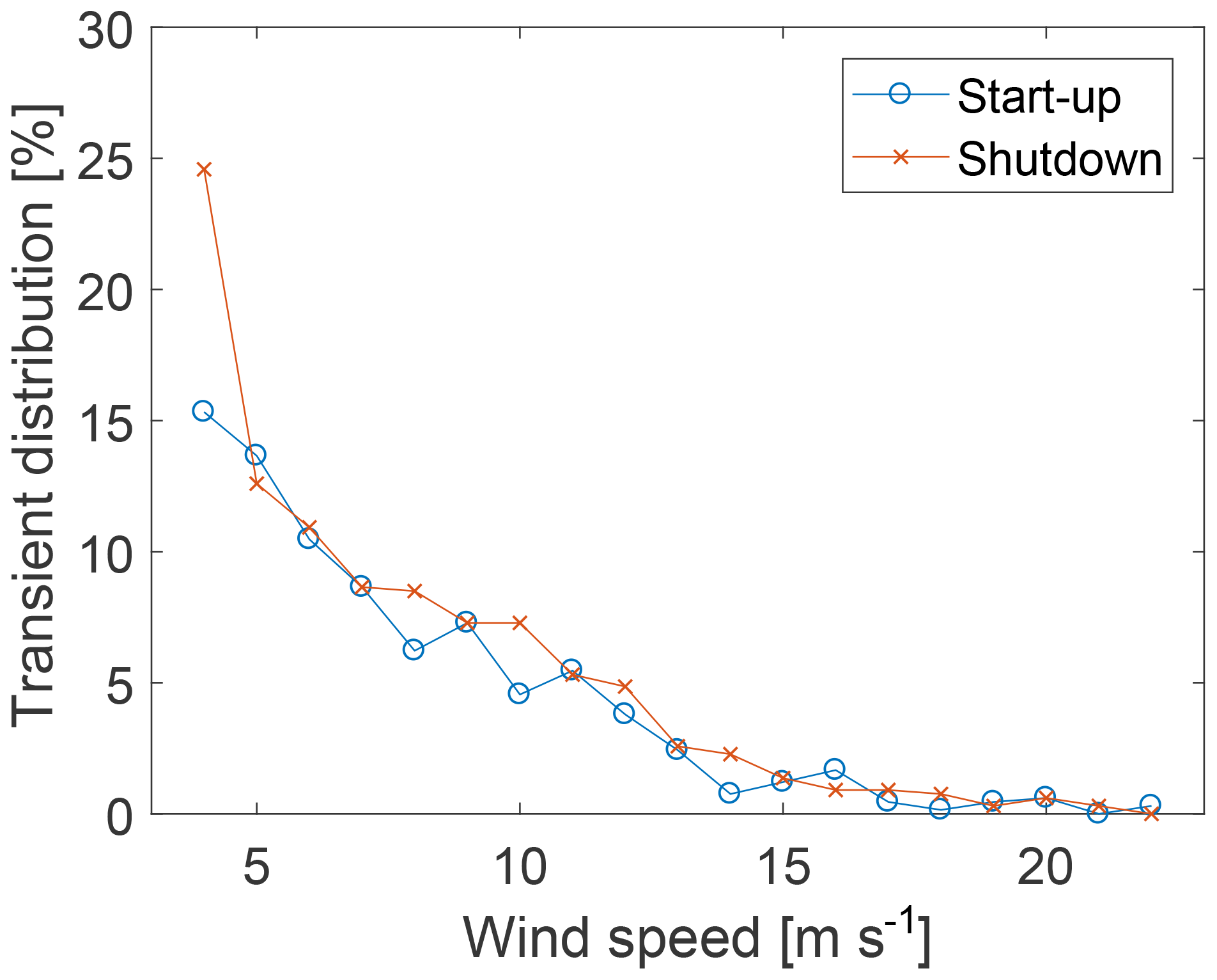
Further scenarios can be included by simulating selected operating conditions (e.g., start-up, shutdown events). When summing up estimations for normal operation with these selected conditions, weights for the probability of the operational state need to be included in Eqs. (5) and (6). The probability of the turbine operating in normal, start-up and shutdown condition varies per wind speed and can be extracted from SCADA data or fault and event logs. For transient events the probability-weighted AEP and DEL can be calculated using the number of transient events per year N_TR,y.

$$\begin{array}{}\text{(7)}& {\displaystyle }& {\displaystyle }{\mathrm{AEP}}_{\mathrm{TR}}=\sum _{i=\mathrm{1}}^{N_{\mathrm{sim}}}{\displaystyle \frac{N_{\mathrm{TR},y}}{N_{\mathrm{sim}}}}\cdot \widehat{P_i}\text{(8)}& {\displaystyle }& {\displaystyle }{\mathrm{DEL}}_{\mathrm{TR}}={\left({\displaystyle \frac{\sum _{i=\mathrm{1}}^{N_{\mathrm{sim}}}\frac{\mathrm{25}\cdot N_{\mathrm{TR},y}}{N_{\mathrm{sim}}}\cdot {\widehat{L}}_{\mathrm{inv},i}}{N_{\sec ,\mathrm{L}}}}\right)}^{\mathrm{1}/m}\end{array}$$

It follows that the probability-weighted AEP and DEL for normal operation can be calculated using Eqs. (9) and (10).

$$\begin{array}{}\text{(9)}& {\displaystyle }& {\displaystyle }{\mathrm{AEP}}_{\mathrm{normal}}=\sum _{i=\mathrm{1}}^{N_{\mathrm{sim}}}{\displaystyle \frac{N_{\mathrm{hours},y}-N_{\mathrm{TR},y}}{N_{\mathrm{sim}}}}\cdot \widehat{P_i}\text{(10)}& {\displaystyle }& {\displaystyle }{\mathrm{DEL}}_{\mathrm{normal}}={\left({\displaystyle \frac{\sum _{i=\mathrm{1}}^{N_{\mathrm{sim}}}\frac{\mathrm{25}\cdot \left(N_{\mathrm{10}\min ,y}-N_{\mathrm{TR},y}\right)}{N_{\mathrm{sim}}}\cdot {\widehat{L}}_{\mathrm{inv},i}}{N_{\sec ,\mathrm{L}}}}\right)}^{\mathrm{1}/m}\end{array}$$

Finally, the weighted AEP and lifetime DELs can simply be added.

$$\begin{array}{}\text{(11)}& {\displaystyle }& {\displaystyle }{\mathrm{AEP}}_{\mathrm{tot}}={\mathrm{AEP}}_{\mathrm{normal}}+{\mathrm{AEP}}_{\mathrm{TR}}\text{(12)}& {\displaystyle }& {\displaystyle }{\mathrm{DEL}}_{\mathrm{tot}}={\mathrm{DEL}}_{\mathrm{normal}}+{\mathrm{DEL}}_{\mathrm{TR}}\end{array}$$

3 Example case

In the following case study the suggested methodology is applied to an offshore wind farm to assess which conditions might be correlated with the component reliability of a main bearing. Main bearings support the rotor shaft, which transfers the aerodynamic torque from the rotor into the gearbox while reducing non-torque loads entering the gearbox (Calderon, 2015). With around USD 150 000 to 300 000 per failure (Dvorak, 2013) unplanned bearing replacement costs are a significant part of the total yearly O & M expenses, which can be approximately USD 645 000 for an offshore 5 MW turbine (Stehly and Beiter, 2020). Figure 4 illustrates the loads considered in this study which are expected to have highest impacts on the main bearing.

The performance, fatigue loads and main bearing lifetime are estimated within the offshore wind farm and compared against the observed failure records. The data used in this study consist of a 5-year SCADA data set with a sampling rate of 10 min. The bearing type observed in this study is a SKF CARB toroidal roller bearing in non-locating position. The main bearing failure records are available from inspection and maintenance reports for the same period. Figure 5 shows the normalized failure rate of the main bearing, i.e., the frequency at which the main bearing has failed. Figure 6 illustrates the inverted time to failure (TTF) $\frac{\mathrm{1}}{\mathrm{TTF}}$, where TTF is defined as the time between start of uptime and start of downtime of the main bearing. A higher inverted TTF therefore indicates earlier failures and shorter lifetimes of the main bearing.

Figure 5 Observed normalized failure rate within wind farm from inspection reports.

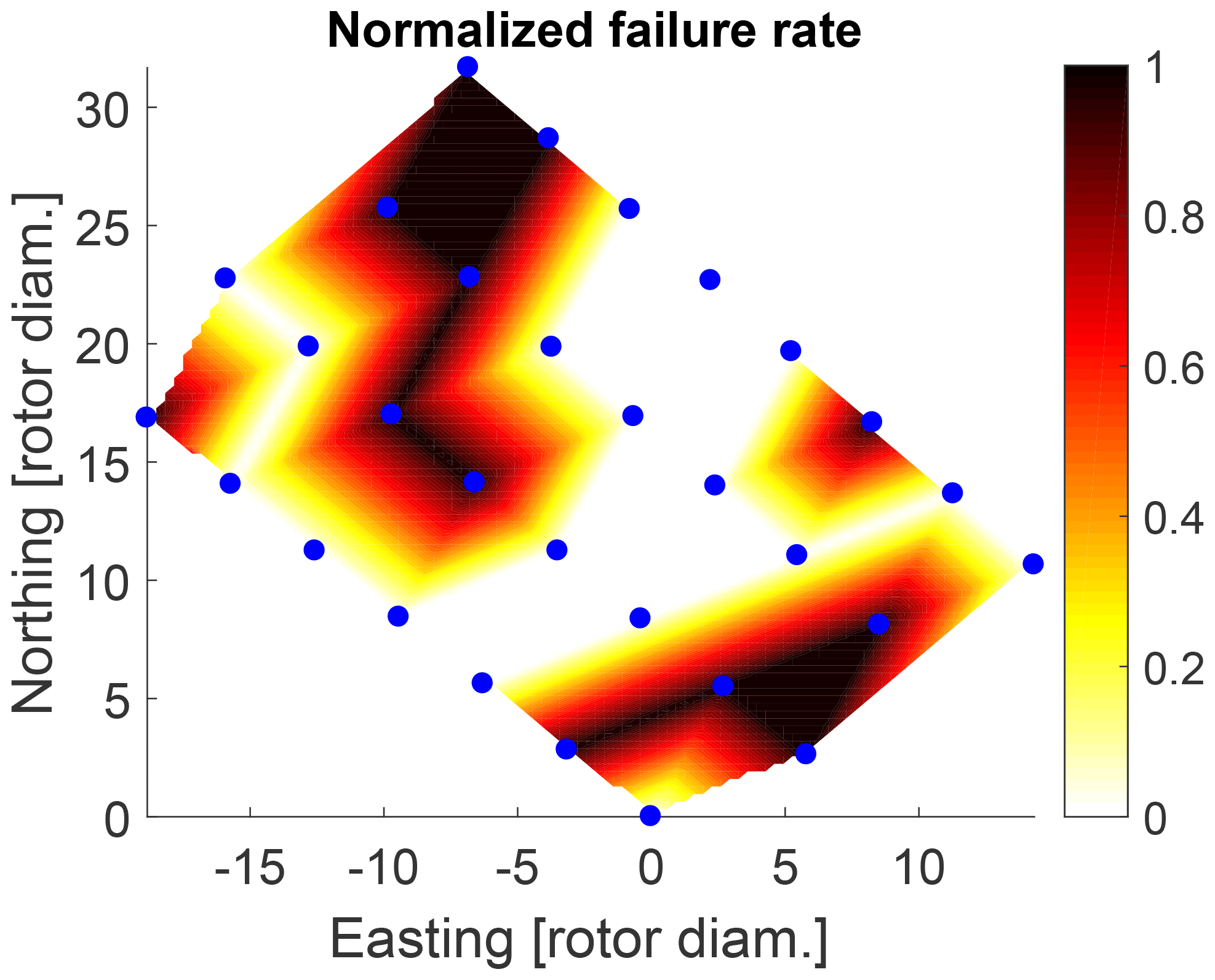
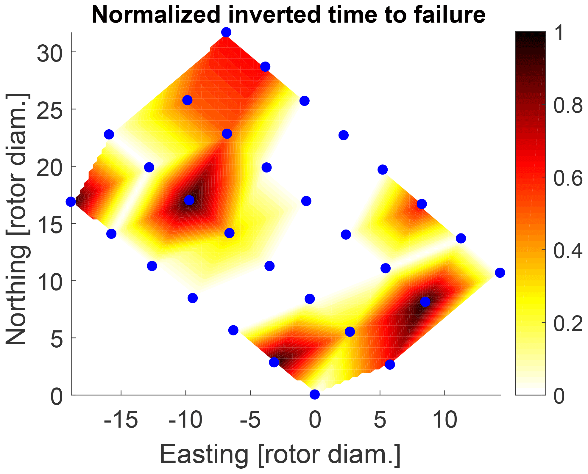
Figure 6 Observed normalized inverted time to failure within wind farm from inspection reports.

3.1 Define variable input space and sample from predefined distributions

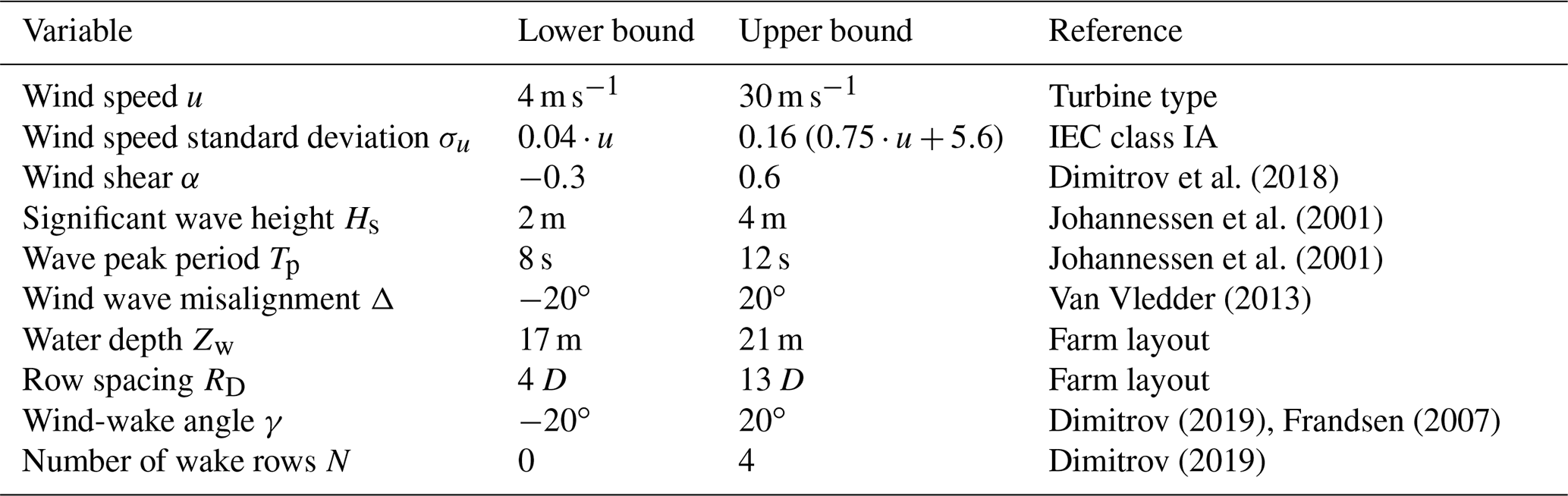
The variable space used for creating the simulation database in this analysis is generated following the approach described in Sect. 2.1. The wind speed is sampled from a uniform distribution ranging between 4 and 30 m s⁻¹ covering the power production range of the wind turbine. For each wind speed sample the remaining variables are drawn from a uniform distribution as well with the selected boundaries as presented in Table 1. It should be noted, however, that the input variables can be sampled following any suitable distribution function without influencing the power and load estimations of the resulting model as the sampling only influences the training process. The boundary functions of the wind speed standard deviation is based on the IEC class IA for offshore conditions and result in a range of 0.16 to 3.89 m s⁻¹. The wind shear boundaries are hard coded based on Dimitrov et al. (2018). Regular waves are modeled as wind-speed-dependent deterministic function for the significant wave height H_s and wave peak period T_p. However, the wind shear and wave conditions are not used as input variables for the surrogate model later on, since the database is simulated using a constant wind shear of 0.14 and the study only observes loads that are expected to not be influenced by waves. The boundaries for the wind wave misalignment Δ are selected based on Van Vledder (2013). The selected boundaries of the water depth and row spacing is based on the wind farm layout. Studies have shown that a turbine does not seem to experience wake condition with wind–wake angles of bigger range than ±25^∘ (Dimitrov, 2019; Frandsen, 2007). Finally, up to four upstream turbines are considered for generating multiple wake conditions based on Dimitrov (2019) showing that including more wake sources does not have a significant effect on the resulting load estimations.

Dimitrov et al. (2018)Johannessen et al. (2001)Johannessen et al. (2001)Van Vledder (2013)Dimitrov (2019)Frandsen (2007)Dimitrov (2019)

Table 1 Sampling conditions of variables considered for creating a simulation database including references used for the selection. D is rotor diameter.

A 2000-point pseudo-Monte Carlo approach based on a low-discrepancy Halton sequence is used to generate the variable space. The resulting samples can be seen in Fig. 7.

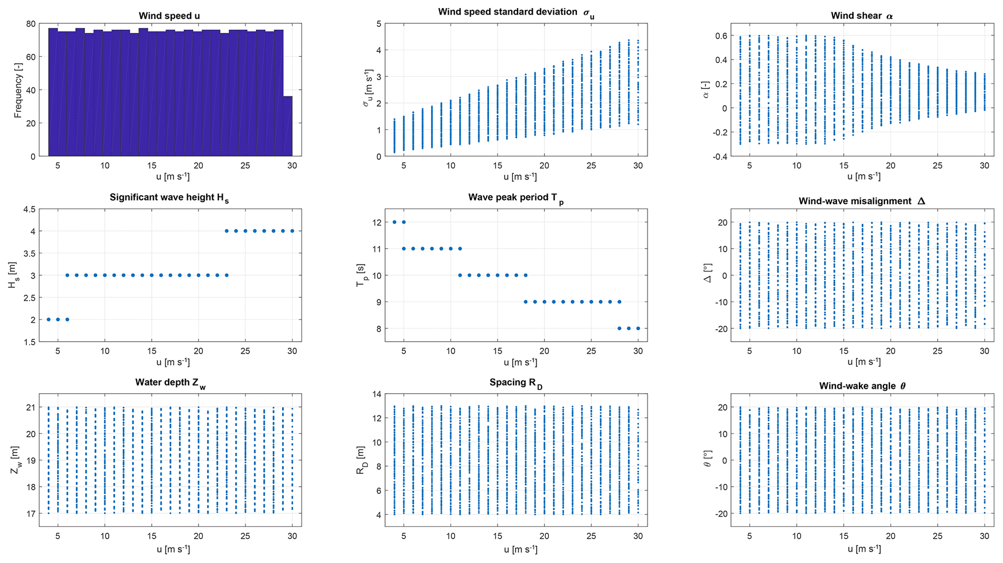
Figure 7 Sample distribution obtained using 2000-point pseudo-Monte Carlo simulation of a 9-dimensional variable space {u, σ_u, α, H_s, T_p, Δ, Z_w, R_D, γ}. All variables are uniformly distributed within defined ranges.

3.2 Aeroelastic simulations for normal operation and transients

A total number of 32 output channels are simulated using the aeroelastic tool HAWC2 (Larsen and Hansen, 2019; Madsen et al., 2020) of the NREL offshore 5 MW reference turbine with a jacket structure (Vorpahl et al., 2011). The simulation settings and turbine model are chosen in order to be representative of the actual wind farm. Turbulence is included with the help of so-called turbulence boxes which are “random realizations of three-dimensional, stationary and homogeneous turbulent wind fields” (Dimitrov, 2019). Under exactly same conditions, the simulated time series will differ from realization to realization due to this effect of the turbulence, which is called the seed-to-seed uncertainty. However, by using a large Monte Carlo sample as in this approach the effect of seed-to-seed uncertainty is reduced (Dimitrov et al., 2018). For simulating the wake effects the dynamic wake meandering (DWM) model (Larsen et al., 2008) is used. It models the wake effects by generating three turbulence boxes for each simulation: the “ambient wind field over the rotor area” (Larsen et al., 2008) is introduced by a standard turbulence box on which the wake deficit, introduced by a micro-turbulence box, is superimposed (Larsen and Hansen, 2019). The relative position of these two turbulence boxes depends on the meandering of the wake which is introduced by a large-scale turbulence field.

The simulations are carried out on each of the 2000 samples and repeated for three different yaw misalignments (−10, 0, +10^∘) including from zero up to four wake sources, which results in a total of 30 000 simulations for each output channel. These time series simulations are carried out for 600 s for normal operation and 250 s for start-up and shutdown operation. A total of 19 start-up simulations are carried out according to the standard DLC 3.1 (IEC, 2019) for each wind speed ranging between 4 and 22 m s⁻¹. Higher wind speeds are not considered as the controller would trigger an emergency shutdown due to an exceedance of the maximum rotor speed. A total of 27 shutdown simulations are carried out according to DLC 4.1 (IEC, 2019) for wind speeds between 4 and 30 m s⁻¹.

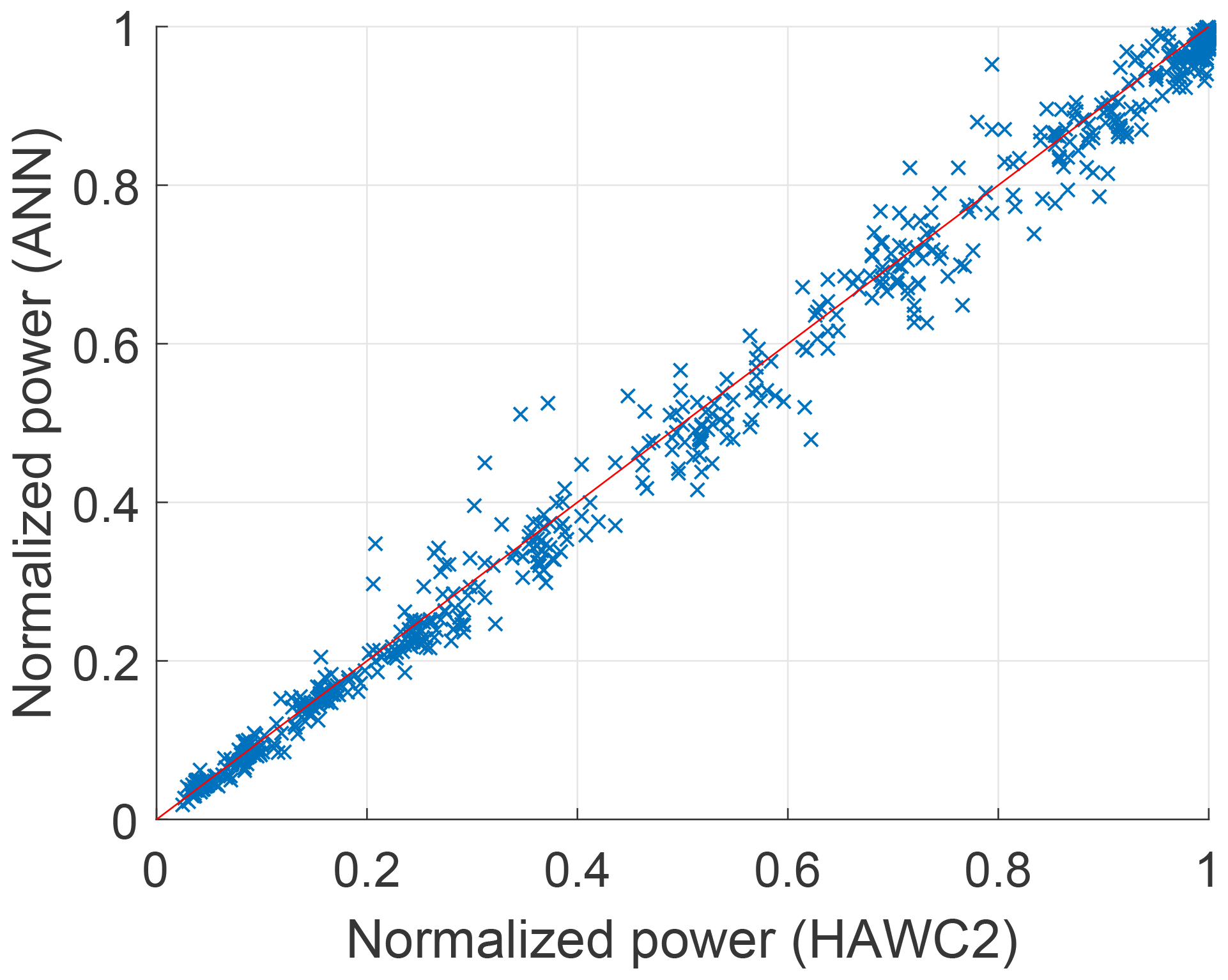
Figure 8 Normalized electrical power P estimated by ANN on test set with respect to normalized power simulated using HAWC2.

Subsequently, the time series are post-processed in order to obtain the desired 10 min statistics, DELs and bearing lifetime. For calculating the DELs of the simulated loads the rainflow counting method (Matsuishi and Endo, 1968) is used with a Wöhler exponent of 4 for the tower top, 8 for the shaft and 10 for the blade root. In order to calculate the lifetime indicator of the main bearing first the time series of the radial force on the main bearing is calculated using the simulated lateral and vertical forces:

$$\begin{array}{}\text{(13)}& F_{\mathrm{r}}=\sqrt{F_{\mathrm{lateral}}^{\mathrm{2}}+F_{\mathrm{vertical}}^{\mathrm{2}}}.\end{array}$$

With the radial force F_r the equivalent dynamic force on the main bearing P_d is calculated using Eq. (3), and next the lifetime L₁₀ is calculated using Eq. (2). A dynamic bearing rating of C=19 600 kN is used, which is the recommended value for the specific bearing type with the specific inner diameter and mass based on the SKF handbook on roller bearings (SKF, 2018). A factor of a₁=0.21 is used corresponding to a 99 % probability of surviving the estimated lifetime. The factor a₂ refers to the bearing material and is set to 1 based on Harris (2001). Finally, the factor a₃ representing the bearing condition, including lubrication and cleanness conditions amongst other things, is set to 1 since the necessary information is not available.

3.3 Train and validate surrogate model (ANN)

The surrogate model is calibrated for estimating 11 output variables S(X) as shown in Fig. 4. However, only estimations for the power, main bearing lifetime, torsional moment at the main bearing and blade-root flapwise bending moment are presented in this paper since the remaining loads show similar resulting patterns.

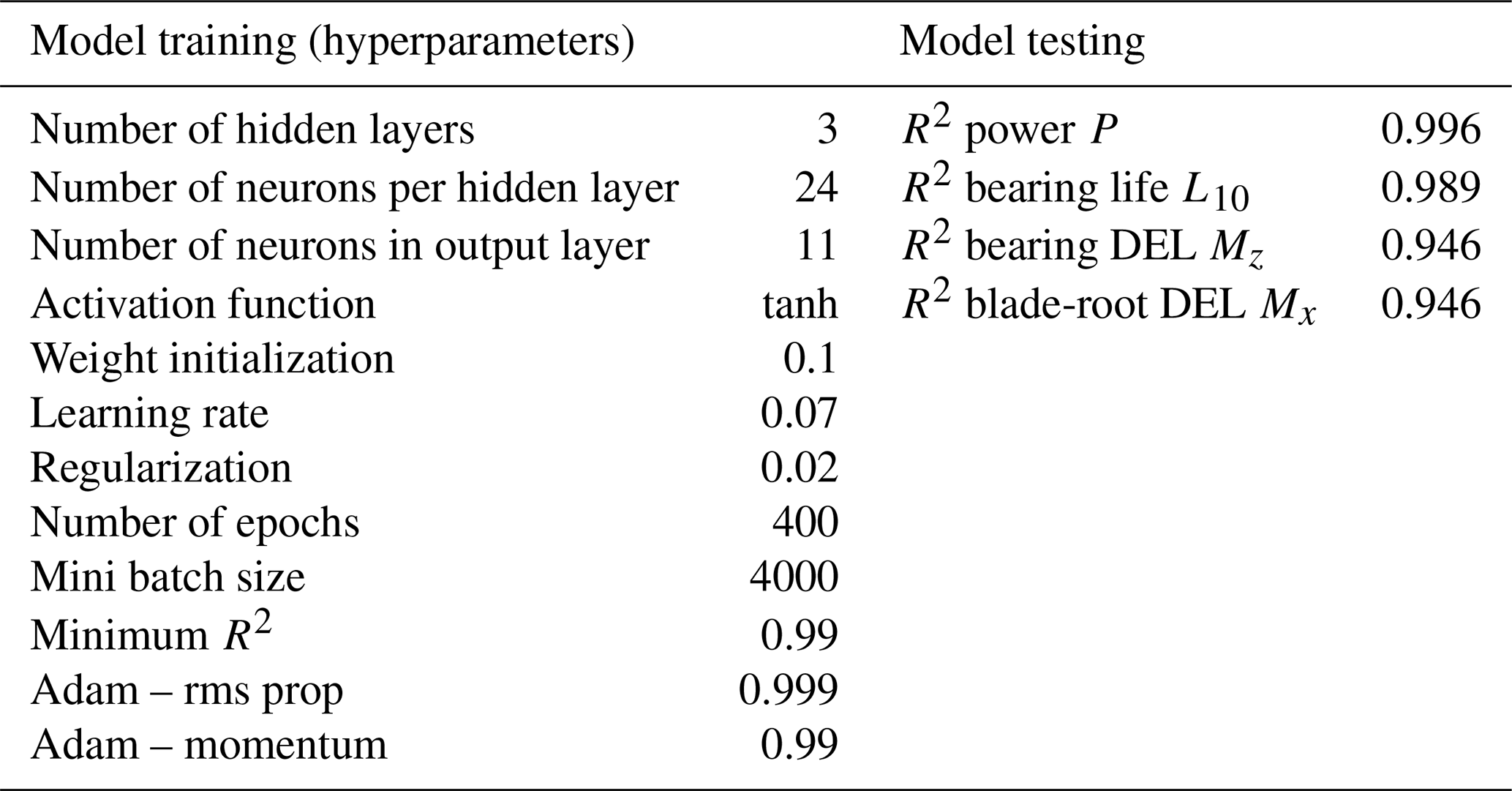
Various ANN architectures have been trained and evaluated on the test set. After hyperparameter tuning the most suitable settings as shown in Table 2 are selected. The data set of 30 000 samples is divided into a 90 % training, 5 % validation and 5 % testing set. Since the number of samples is relatively large, using other ratios for the train–test split did not affect the model performance. The model parameters are estimated with error back-propagation using the adaptive moment estimation (Adam) (Kingma and Ba, 2014) as an adaptive learning rate optimization algorithm for minimizing the cost function J(W, b). Instead of calculating the cost function for the complete data set, at each iteration a mini-batch optimization is used in order to increase computational efficiency and to achieve a more robust convergence. Furthermore, a regularization factor is included in the parameter estimations to avoid overfitting to the training data.

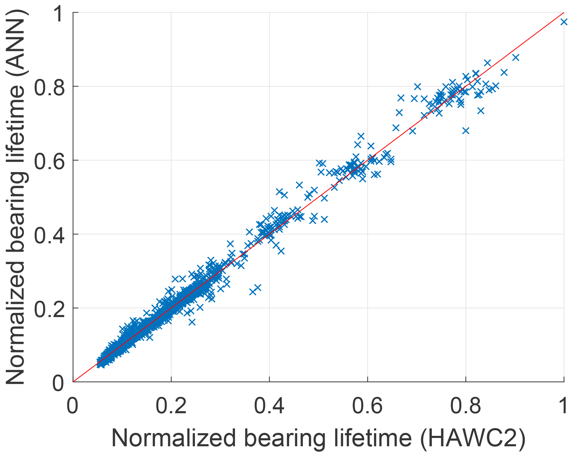
Figure 9 Normalized bearing lifetime L₁₀ estimated by ANN on test set with respect to normalized bearing lifetime simulated using HAWC2.

Figure 10 Site-specific wind rose calculated from free-stream SCADA data.

The model performance is then evaluated by calculating the accuracy of the model predictions on the test set (see Table 2). Figures 8 and 9 show a one-to-one plot for the estimated power P and main bearing lifetime L₁₀ on the test set against the simulation data from HAWC2.

3.4 Site-specific estimations

In order to exclude outliers from the SCADA data, the OpenOA filtering toolkit developed at NREL (Optis et al., 2019) is applied. Figure 10 shows the probability of each wind direction sector that is obtained from the filtered free-stream SCADA data.

Table 2 Hyperparameter of ANN used as surrogate model and accuracy of the model predictions on the test set.

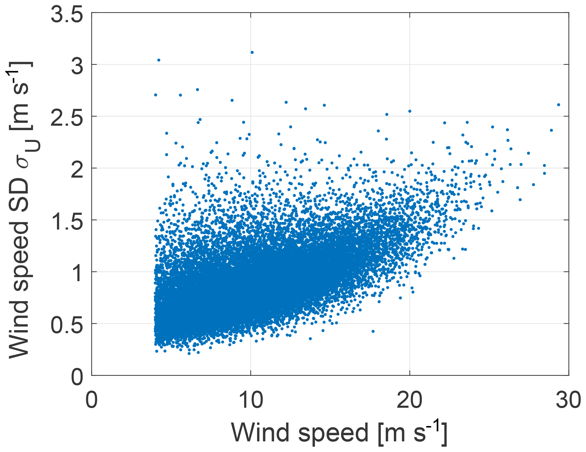
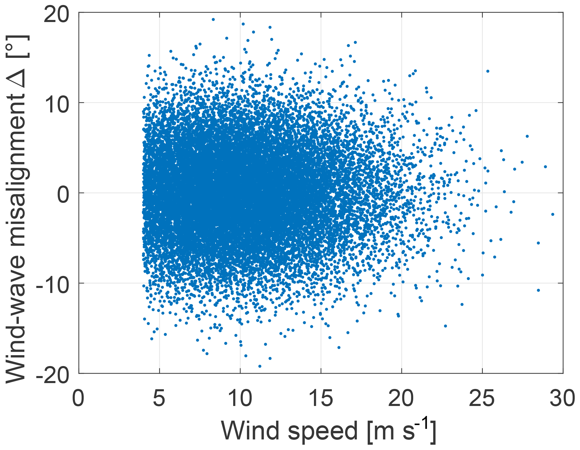
For each wind direction sector a Weibull distribution is fit to the wind speed measurements, and a lognormal distribution is fit per wind speed bin to the wind speed standard deviation measurements. The wind–wave misalignment which describes the difference between wind direction and wave direction of wind-generated wave can depend on the wind speed and significant wave height (Van Vledder, 2013). However, since the bearing in the rotor is almost not affected by the wave conditions the wind–wave misalignment is assumed to be normally distributed with a mean μ=0 and standard deviation σ=5 based on presented distributions in Van Vledder (2013). The three above site-specific input variables of the environmental conditions X_amb are generated using a 20 000-point pseudo-Monte Carlo simulation based on Sobol sequences following the approach described in Sect. 2.4. The final input samples for the surrogate model are shown in Fig. 11 for the wind speed, Fig. 12 for the wind speed standard deviation and Fig. 13 for the wind–wave misalignment.

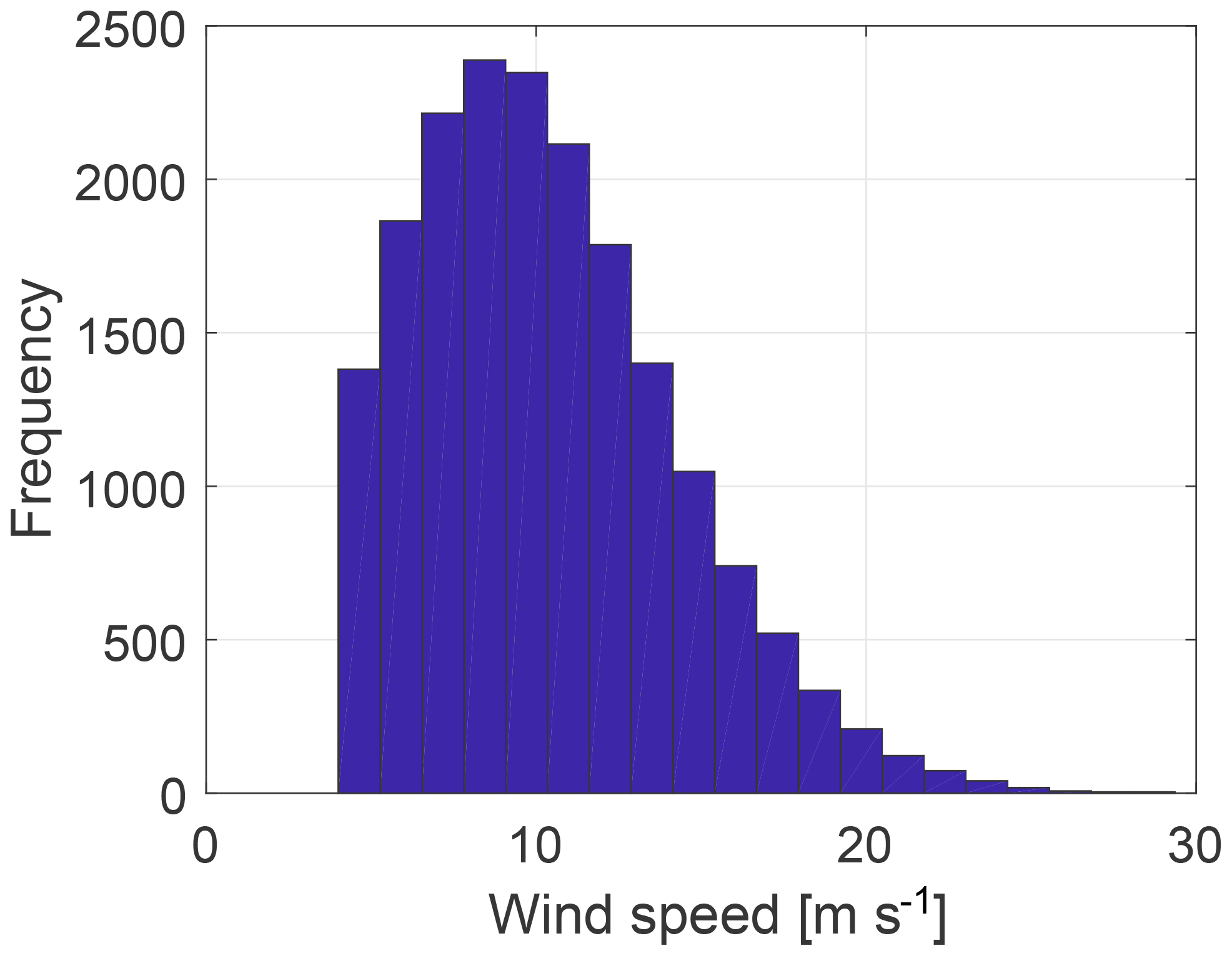
Figure 11 Site-specific wind speed sampled from Weibull distribution from free-stream SCADA data.

Figure 12 Sampled wind speed standard deviation taken from SCADA.

Figure 13 Sampled wind wave misalignment.

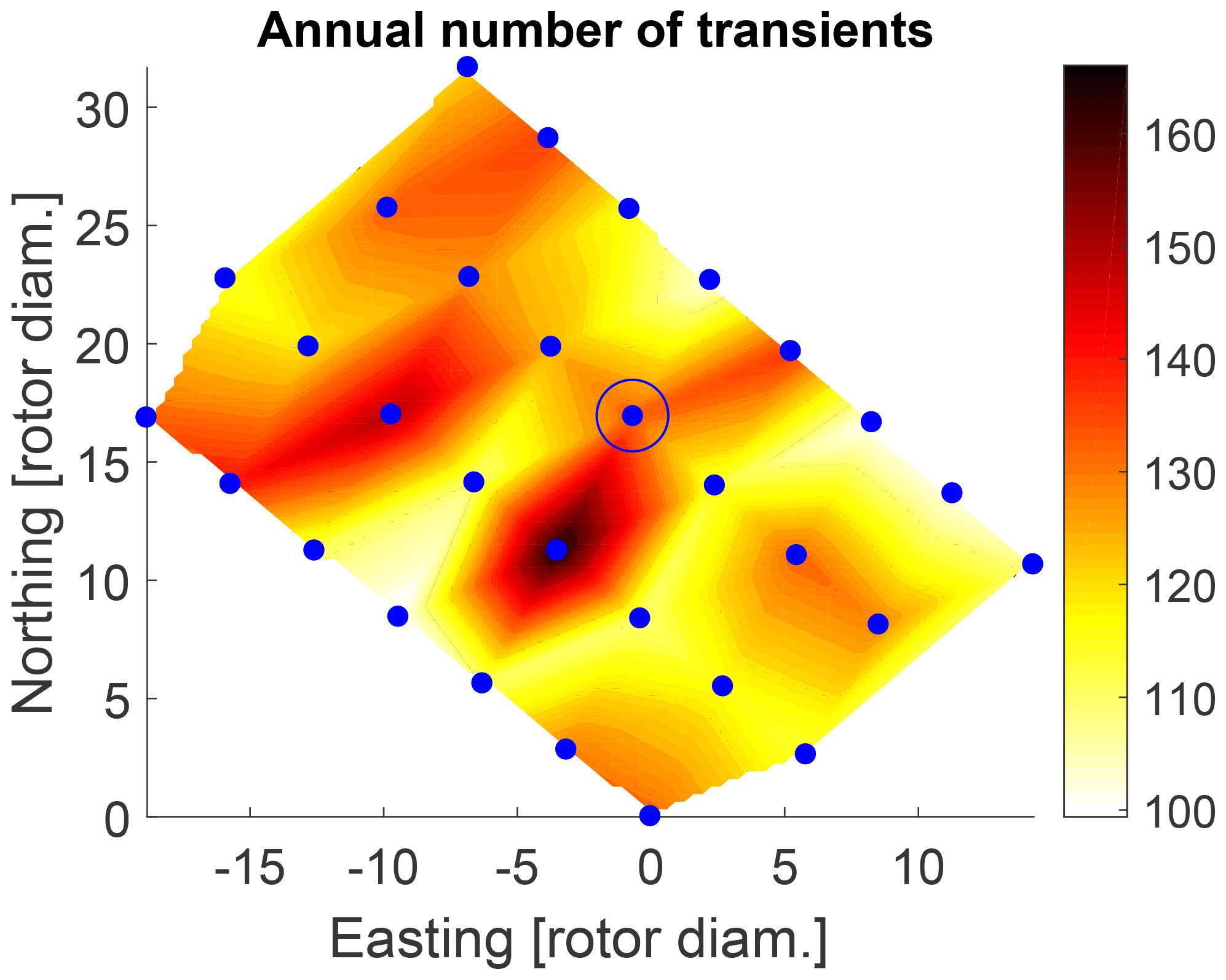
For summing up the model predictions of both normal and transient operation, the model predictions are weighted according to their probability of operational state. Figure 15 shows the probabilities of start-up and shutdown events for an example turbine. The annual number of transients over the whole wind farm can be seen in Fig. 14.

Figure 14 Number of start-up and shutdown events within wind farm from SCADA data.

Figure 15 Example for percentage of start-up and shutdown events per wind speed for Turbine 19 (marked with blue circle in Fig. 14).

3.5 Operation-state weighted sum

The final resulting probability-weighted outputs for the offshore wind farm for the AEP, main bearing lifetime, blade-root flapwise DEL and torsional bearing DEL are shown in Figs. 16 to 19. These results should be analyzed in comparison with Figs. 5 and 6, which show the actual failure maps over the wind farm.

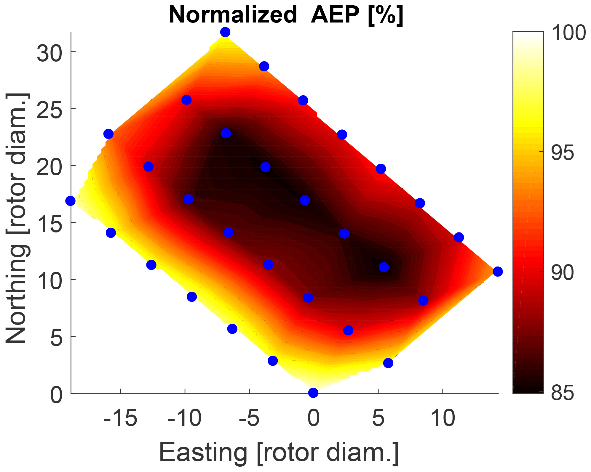
Figure 16 Estimated normalized AEP within wind farm for normal operation including start-up and shutdown events.

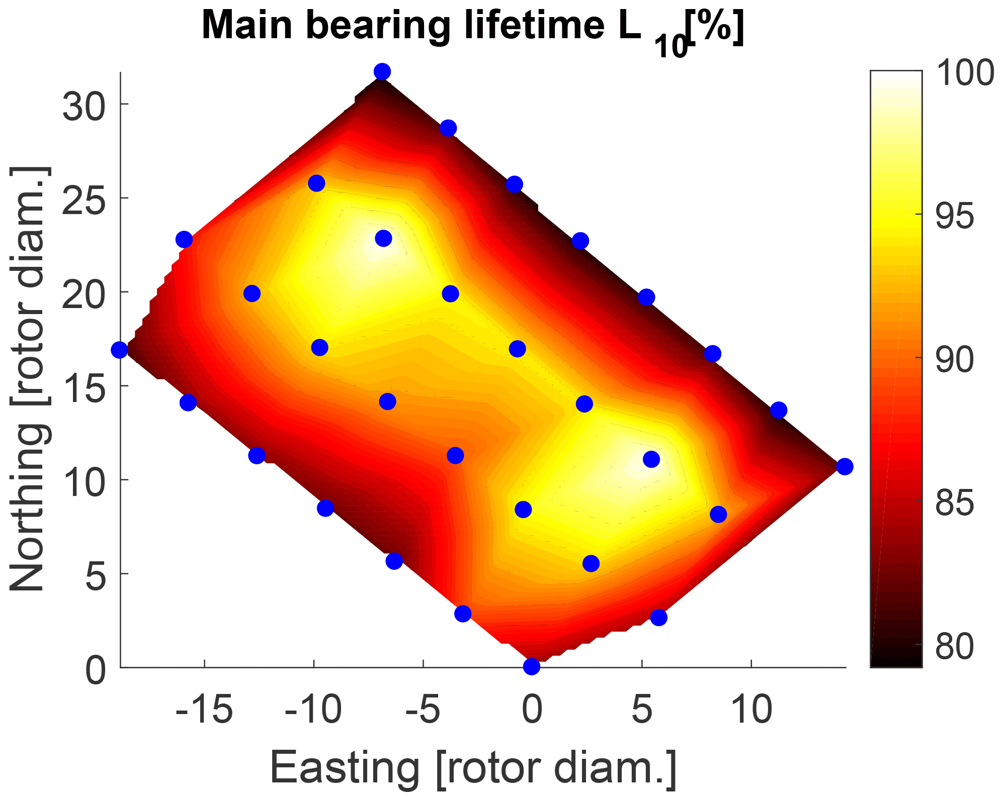
Figure 17 Estimated normalized bearing lifetime within wind farm for normal operation including start-up and shutdown events.

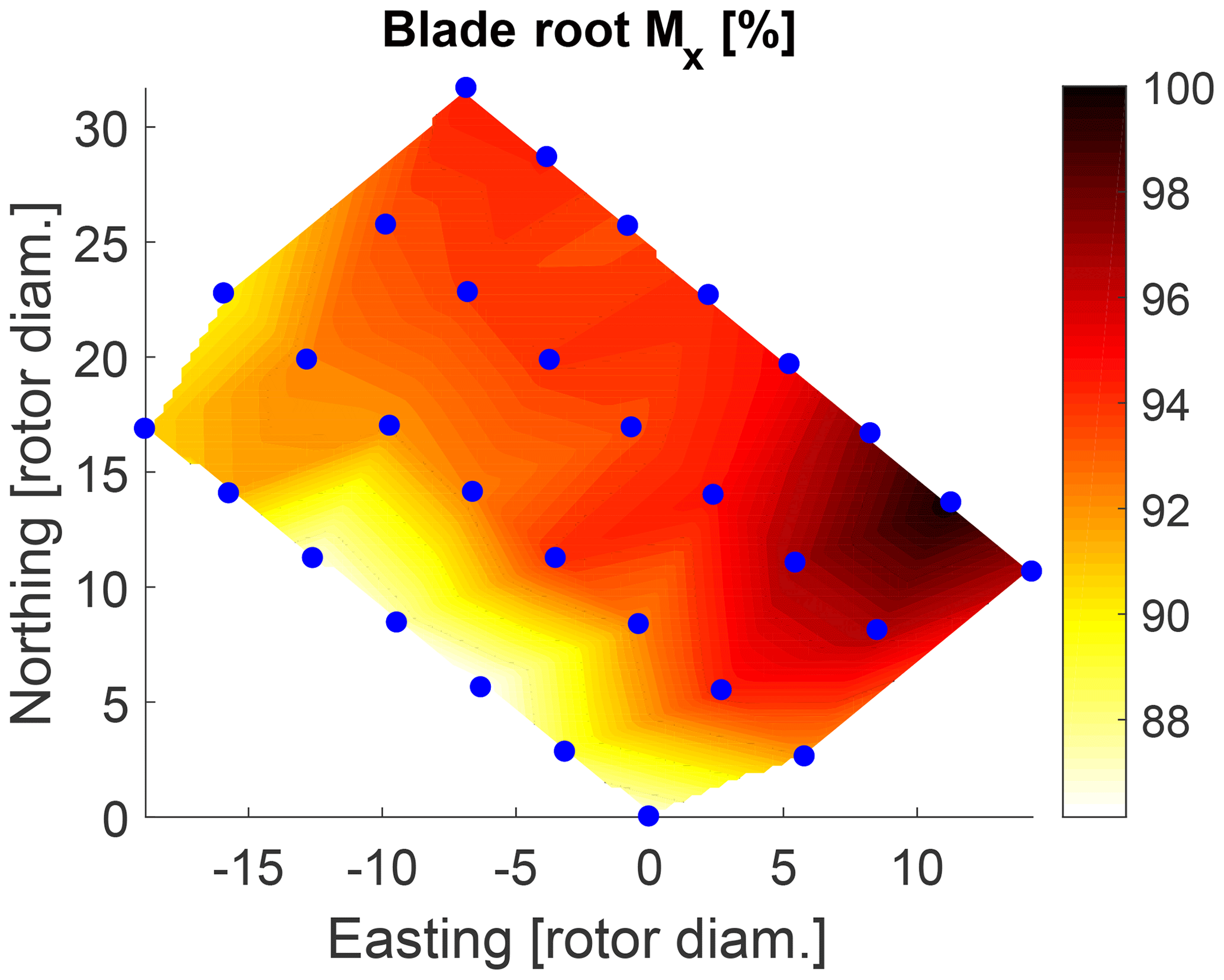
Figure 18 Estimated normalized blade-root flapwise DEL within wind farm for normal operation including start-up and shutdown events.

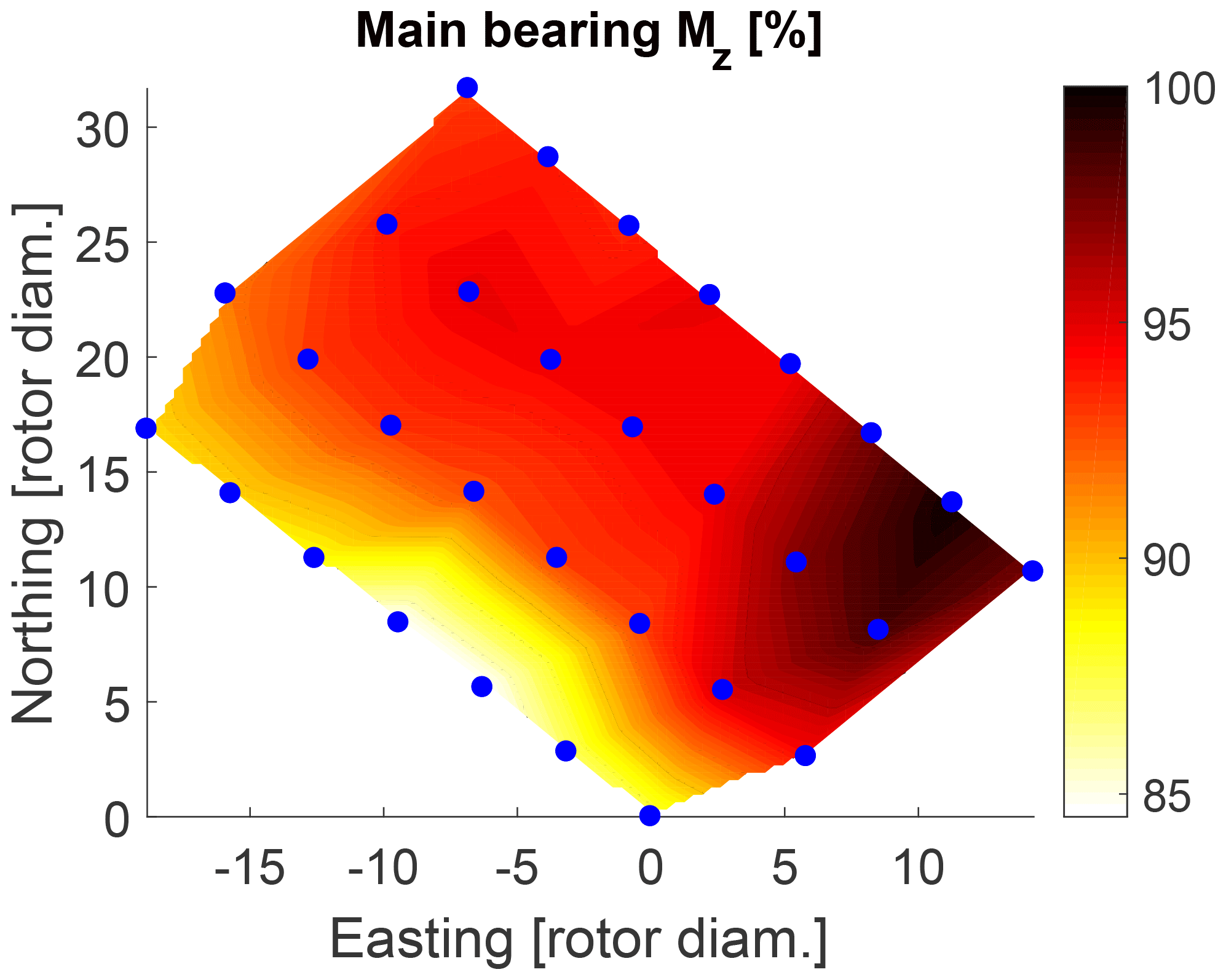
Figure 19 Estimated normalized DEL of torsional moment on main bearing within wind farm for normal operation including start-up and shutdown events.

For validation purposes, the surrogate model is used to estimate the power time series of each turbine for a time period of 1 year under normal operation and compared against the measured power from the SCADA system (see Fig. 20). The coefficient of determination R² of the power predictions for the single turbines ranges between 0.89 and 0.93 (see Fig. 21). The power for the northernmost turbine could not be calculated since its measurement data were not available. The AEP is calculated for each turbine showing a relative error between the measured and the estimated normal behavior AEP between 0.1 % and 3.4 % (see Fig. 22). The mean relative error of the AEP estimation for all 29 turbines is 1.5 %.

Figure 20 Comparison of measured power time series from SCADA data (solid line) and predicted time series from the ANN (dashed line) for an example turbine.

Figure 21 Coefficient of determination R² of power time series prediction under normal operation.

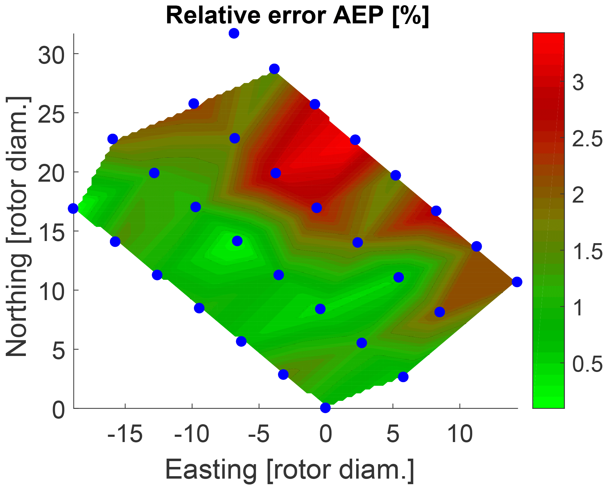
Figure 22 Relative error between measured AEP from SCADA data and estimated AEP within wind farm.

4 Discussion

The results show that the ANN is able to accurately model the simulated power, DEL and L₁₀ with a coefficient of determination R² between 0.95 and 0.99. The validation of the estimated time series against the measured 10 min SCADA statistics shows that the power is modeled with a mean prediction error of 1.5 % and an average R² value of 0.91. The time series predictions show a consistent offset at rated power (see Fig. 20). A reason for the difference might be that a generic model had to be used since the more accurate model by the turbine manufacturer was not available. Furthermore, higher uncertainty can be observed for the eastern turbines, i.e., the turbines which are more often experiencing wake conditions (see Fig. 21).

The surrogate modeling approach discussed in this study includes several assumptions and uncertainties which are propagated to the final predictions. The uncertainties in the final model predictions depend on various matters, such as the defined variable space, the wake model used, the selection of environmental input parameters, assumptions for modeling the wake effects in the surrogate model and the surrogate model performance. Investigating different model setups has shown that the results are sensitive towards the way in which the wake is observed (i.e., size of wind direction sector) and how wake is defined as input variables (i.e., considering upstream turbines resulting in most conservative estimates). Despite these uncertainties and data limitations, the model is able to capture the relative differences in the power and fatigue load accumulation over the wind farm well.

The DEL predictions of the blade-root flapwise bending moment and the torsional bearing moment in Figs. 18 and 19 seem to increase when moving east within the farm. This is expected as those turbines are experiencing multiple wake conditions with prevailing wind from southwest. The model predictions in Fig. 16 show that the highest AEP is observed at turbines positioned in the outer border of the wind farm. This makes sense as well because these turbines are more likely to experience free-stream conditions and therefore higher wind speeds as compared to inner positioned turbines. Comparing the AEP map (Fig. 16) with the main bearing lifetime predictions (Fig. 17), it can be seen that those mentioned outer turbines with increased AEP are estimated to have a shorter main bearing lifetime. This indicates the possible correlation that turbines within a wind farm that are located at positions of higher expected AEP might be prone to experiencing earlier main bearing failures as compared to the rest of the wind farm.

Although the lifetime L₁₀ is a rather simplistic indicator and misses additional condition information (e.g., about the lubrication status), the lifetime estimations (Fig. 17) do not contradict the observed main bearing lifetime (Fig. 6): while turbines at the outer border of the wind farm are estimated to have a shorter main bearing lifetime, most turbines that were observed to have a premature failure already within the first 3 years of operation are positioned on the border as well, with only one exception. A comparison of the observed failure rates (Fig. 5) with the DEL estimations does not show any clear patterns or correlations, except that 2 out of 12 turbines with higher failure rates are positioned in the region of highest estimated blade-root DEL M_x and main bearing DEL M_z. Furthermore, there does not seem to be an obvious connection between the prevailing wind direction of around 240^∘ (Fig. 10) and the failures.

The reference value by SKF for the required L₁₀ lifetime of a wind turbine roller bearing ranges between 30 000 and 100 000 h of operation (SKF, 2018), i.e., that 10 % of a sufficiently large number of identical main bearings under identical conditions are expected to fail within the first 3.4 to 11.4 years of operation. Given that already 40 % of the turbines of the studied wind farm have experienced a main bearing failure by the sixth year of operation, the observations might indicate an unexpectedly high failure rate. However, when interpreting the results and drawing conclusions about possible correlations, it is also important to keep in mind the limitations of the model and data. Since the number of recorded failures is rather limited, it might not be representative of the underlying main bearing failure statistics. More observations are necessary in order to demonstrate a statistically significant difference in the averages of the main bearing lifetime (mean TTF) per turbine or subgroup of turbines. It becomes clear that more failure data from the same wind farm as well as from other wind farms are needed to validate and generalize the possible relationships. Furthermore, the observed main bearing failures are not necessarily fatigue-induced and might have been caused by other factors that are not included in the analysis (e.g., faults during manufacturing process). Finally, the case study shows model estimations for a limited number of operational states, i.e., normal operation and start-up and shutdown behavior. Other operational states or wind conditions could have an impact on the main bearing reliability (i.e., parking, curtailment, wake steering, wind gusts, faults, emergency shutdown).

5 Conclusions

This study presents a procedure that makes it possible to correlate performance and loading conditions within a wind farm with its component reliability in a computationally efficient way. It can be used for assessing the health state of turbines in a wind farm and for getting a better understanding and definition of how fatigue loading can lead to failures. In the demonstration on an offshore wind farm with the focus on observed main bearing failures, the following was found:

• The ANN is able to predict the electrical power, blade-root flapwise DEL, torsional bearing DEL and main bearing lifetime accurately with an R² value of higher than 0.95 compared to the simulated values.

• The validation of the estimated power time series against the 10 min SCADA power signals shows that the surrogate model is able to capture the power performance relatively well with a 1.5 % average error in the AEP prediction.

• Turbines at the border of the wind farm are estimated to have a shorter bearing lifetime. These estimations do not contradict the observed bearing lifetime from inspection and maintenance reports.

• A clear connection between the load estimations and failure observations could not be confirmed.

• Further future work can expand the case study to more operating states which could affect the bearing reliability, such as parking conditions. Also, more valuable insights can be gained by including other types of data sources, e.g., SCADA alarms.

Finally, the analysis stresses that more failure data are needed in order to validate and generalize the suggested approach and its associated findings.