An improved second-order dynamic stall model for wind turbine airfoils

Robust and accurate dynamic stall modeling remains one of the most difficult tasks in wind turbine load calculations despite its long research effort in the past. In the present paper, a new second-order dynamic stall model is developed with the main aim to model the higher harmonics of the vortex shedding while retaining its robustness for various flow conditions and airfoils. Comprehensive investigations and tests are performed at various flow conditions. The occurring physical characteristics for each case are discussed and evaluated in the present studies. The improved model is also tested on four different airfoils with different relative thicknesses. The validation against measurement data demonstrates that the improved model is able to reproduce the dynamic polar accurately without airfoil-specific parameter calibration for each investigated flow condition and airfoil. This can deliver further benefits to industrial applications where experimental/reference data for calibrating the model are not always available.

1 Introduction

An accurate prediction of wind turbine blade loads is influenced by many parameters including 3D and unsteady effects. The first mainly occurs in the root and tip areas of the blade due to radial flow and induced velocity influences, respectively (Bangga, 2018). The latter can occur due to variation in the inflow conditions caused by yaw misalignment, wind turbulence, shear and gusts, tower shadow, and aeroelastic effects of the blade. The abovementioned phenomena may result in dynamic stall (DS). Experimental studies (Martin et al., 1974; Carr et al., 1977; McAlister et al., 1978) showed that the aerodynamic forces can differ significantly in comparison to the static condition. DS is often initiated by the generation of a leading edge vortex (LEV), which increases the positive circulation effect on the airfoil suction side, causing delayed stall (Bangga, 2019). This intense leading edge vortex is convected downstream along the airfoil towards the trailing edge. At the same time, the lift force increases significantly, and the pitching moment becomes more negative compared to the static values. A significant drag increase is observed at large angles of attack. An example is shown in Fig. 1. Afterwards, a trailing edge vortex (TEV) with opposite rotational direction than LEV is formed, which pushes the leading edge vortex towards the wake area. This onset may result in a significant drop of the lift coefficient (C_L) and can be dangerous for the blade structure itself, although dynamic stall also generally enhances aerodynamic damping.

Figure 1 Typical dynamic stall behavior of S801 airfoil. Data obtained from Ramsay et al. (1996).

To model the behavior of the airfoil under these situations, semiempirical models can be used. The models are known to produce reasonable results without any notable increase in computational effort. Despite that, these models usually cannot reproduce higher harmonics of the load fluctuations. Furthermore, the applied constants shall be adjusted according to the flow conditions and airfoils. Leishman and Beddoes (LB) (Leishman and Beddoes, 1989) have developed a model for dynamic stall combining the flow delay effects of attached flow with an approximate representation of the development and effect of separation (Larsen et al., 2007). This model was developed for helicopter applications and therefore includes a fairly elaborate representation of the nonstationary attached flow depending on the Mach number and a rather complex structure of the equations representing the time delays (Larsen et al., 2007). Hansen et al. (2004) simplified the model for wind turbine applications by removing the consideration of compressibility effects and the leading edge separation. The latter was argued because the relative thickness of wind turbine airfoil is typically no less than 15 %. This model was called the Risø model in Larsen et al. (2007). Examples of the other models are given by Øye (Øye, 1991), Tran and Petot (Tran and Petot, 1980) (ONERA model), and Tarzanin (Boeing Vertol model) (Tarzanin, 1972). To better model the vortex shedding characteristics at large angles of attack, second-order dynamic stall models were introduced. An example of this model was given by Snel (1997) which makes use of the difference between the inviscid and viscous static polar data as a main forcing term for the dynamic polar reconstruction, in contrast to the LB model that uses the changes of the angle of attack over the time. An improved version of the Snel model was proposed recently by Adema et al. (2020) to cover for the increased shedding effects in the downstroke phase. All abovementioned models employ the static polar data and dynamic flow parameters as the input needed for the dynamic polar reconstruction. Then, the models compute the dynamic force difference required for the reconstruction process.

Although many studies have been dedicated to dynamic stall modeling (Gupta and Leishman, 2006; Larsen et al., 2007; Adema et al., 2020; Elgammi and Sant, 2016; Wang and Zhao, 2015; Sheng et al., 2006; Galbraith, 2007; Sheng et al., 2008), engineering calculations in the industry are still relying on the very basic classical dynamic stall models such as the Leishman–Beddoes and Snel models. The reason is the simplicity to tune in the models for different airfoils and for different flow conditions. Therefore, one major key for a model to be used in industrial applications is robustness of the model itself; i.e., the model is easy to apply with a small number of well-defined user parameters. One of the purposes of this paper is to document widely used dynamic stall models in research and industries. These include the first-order LB model and the second-order Snel model. A very recently improved Snel model according to Adema et al. (2020) will also be evaluated. The mathematical formulations of these models will be presented in this report. Weaknesses of existing dynamic stall modeling shall be identified, and possible corrections to those limitations will be described. Finally, a new second-order dynamic stall modeling will be proposed that is able to model not only the second-order lift and drag forces, but also the pitching moment along with calculation examples in comparison to experimental data for different airfoils and flow conditions.

The paper is organized as follows. Section 2 describes the mathematical formulation of existing dynamic stall models and the new model developed in this work. Then, in Sect. 3 assessments are carried out on the performance of the second-order dynamic stall models in comparison with measurement data. The new model is further tested at various flow conditions and to examine its robustness on four different airfoils without further calibrating the constants. Finally, all results will be concluded in Sect. 4.

2 Mathematical formulations

In this section the mathematical formulations of each model are described in detail. The reasons are mainly to provide information on how each model was employed and to gain deeper insights for further developing the new model. Note that each existing model was developed by different authors; thus different symbols and formulation methods were adopted in those publications (Beddoes, 1982; Leishman, 1988; Leishman and Beddoes, 1989; Snel, 1997; Adema et al., 2020). In this paper, all models are described in a consistent way for clarity and for an easier interpretation and implementation process.

2.1 Leishman–Beddoes model

The original Leishman–Beddoes model is composed of three main contributions representing various flow regimes: (1) unsteady attached flow, (2) unsteady separated flow and (3) dynamic stall. The present section will elaborate the mathematical description and its physical interpretation of each module. Figure 2 illustrates several main parameters needed for modeling the dynamic stall characteristics.

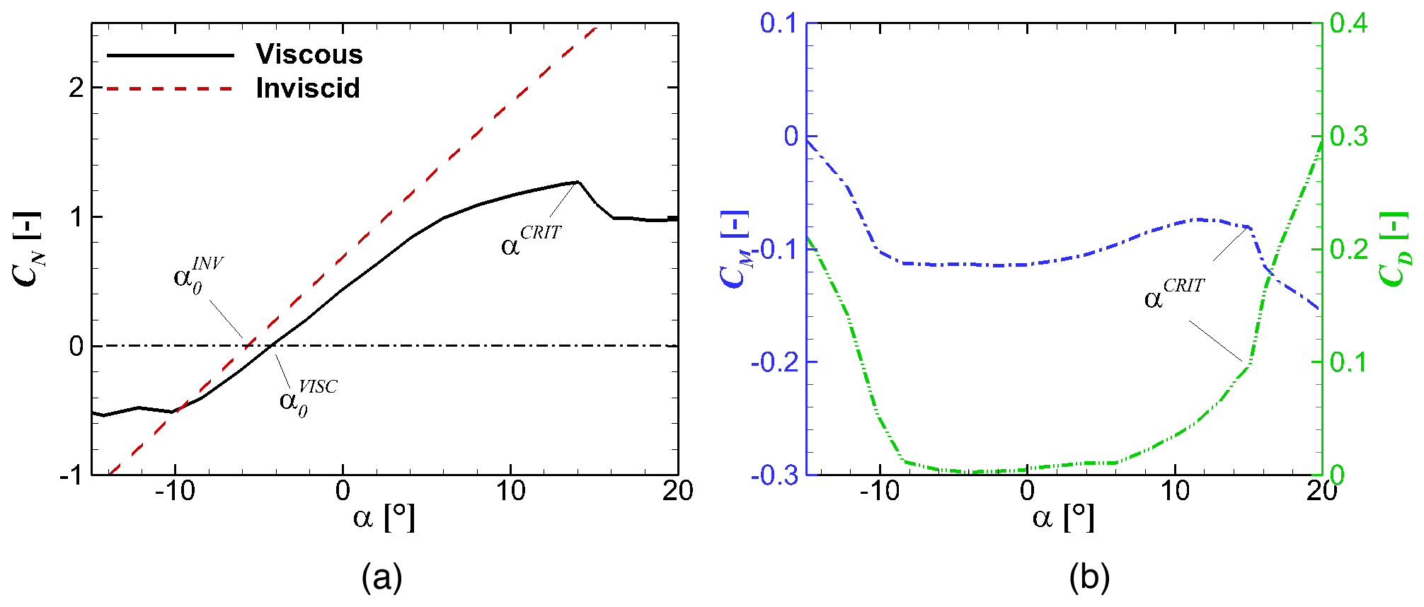
Figure 2 Illustration of the main aerodynamic parameters needed for modeling the dynamic stall characteristics.

2.1.1 Unsteady attached flow

In this module, the unsteady aerodynamic response of the loads is represented by the time delay effects. The indical formulas were constructed based on the work of Beddoes (1982) and have been refined by Leishman (1988). The loads are assumed to originate from two main sources: one for the initial noncirculatory loading from the piston theory and another for the circulatory loading which builds up quickly to the steady-state value (Leishman and Beddoes, 1989). In the formulation, the relative distance traveled by the airfoil in terms of semi-chords is represented by $s=\mathrm{2}Vt/c$, which can also be used to describe the nondimensional time. Note that V, t and c are free-stream wind speed, time and chord length, respectively. For a continuously changing angle of attack α_n, the effective angle of attack (${\mathit{\alpha }}_{{\mathrm{e}}_n}$) can be represented as

$$\begin{array}{}\text{(1)}& {\mathit{\alpha }}_{{\mathrm{e}}_n}={\mathit{\alpha }}_n-X_n-Y_n,\end{array}$$

where n is the current sample time. The last two terms describe the deficiency functions that are given by

$$\begin{array}{}\text{(2)}& {\displaystyle }& {\displaystyle }{X}_n=X_{n-\mathrm{1}}\exp \left(-b_{\mathrm{1}}{\mathit{\beta }}^{\mathrm{2}}\mathrm{\Delta }s\right)+A_{\mathrm{1}}\mathrm{\Delta }{\mathit{\alpha }}_n\exp \left(-b_{\mathrm{1}}{\mathit{\beta }}^{\mathrm{2}}\mathrm{\Delta }s/\mathrm{2}\right),\text{(3)}& {\displaystyle }& {\displaystyle }{Y}_n=Y_{n-\mathrm{1}}\exp \left(-b_{\mathrm{2}}{\mathit{\beta }}^{\mathrm{2}}\mathrm{\Delta }s\right)+A_{\mathrm{2}}\mathrm{\Delta }{\mathit{\alpha }}_n\exp \left(-b_{\mathrm{2}}{\mathit{\beta }}^{\mathrm{2}}\mathrm{\Delta }s/\mathrm{2}\right),\end{array}$$

where

$$\begin{array}{}\text{(4)}& {\displaystyle }& {\displaystyle }\mathrm{\Delta }{\mathit{\alpha }}_n={\mathit{\alpha }}_{n+\mathrm{1}}-{\mathit{\alpha }}_n,\text{(5)}& {\displaystyle }& {\displaystyle }\mathrm{\Delta }s=s_n-s_{n-\mathrm{1}}.\end{array}$$

In these equations, b₁, b₂, A₁ and A₂ are constants. The variable β represents the compressibility effects and is formulated as $\mathit{\beta }=\sqrt{\mathrm{1}-M^{\mathrm{2}}}$. Because information about the previous cycle is needed in the formulations, initializations are required. The solution needs to develop for a certain time until convergence of the resulting unsteady loads is obtained.

The circulatory normal force due to an accumulating series of step inputs in angle of attack can be obtained using

$$\begin{array}{}\text{(6)}& C_{{\mathrm{N}}_n}^{\mathrm{C}}={\displaystyle \frac{\mathrm{d}{C}_{\mathrm{N}}}{\mathrm{d}\mathit{\alpha }}}\left({\mathit{\alpha }}_{{\mathrm{e}}_n}-{\mathit{\alpha }}_{\mathrm{0}}^{\mathrm{INV}}\right).\end{array}$$

The variable ${\mathit{\alpha }}_{{\mathrm{0}}_{\mathrm{INV}}}$ is the angle of attack for zero inviscid normal force. The original formulation of the model disregarded the use of ${\mathit{\alpha }}_{\mathrm{0}}^{\mathrm{INV}}$. However, this term is important when the airfoil has a finite camber. This has been pointed out as well by Hansen et al. (2004).

The noncirculatory (impulsive) normal force is obtained by

$$\begin{array}{}\text{(7)}& C_{{\mathrm{N}}_n}^{\mathrm{I}}={\displaystyle \frac{\mathrm{4}{K}_{\mathit{\alpha }}{T}_{\mathrm{I}}}{M}}\left({\displaystyle \frac{\mathrm{\Delta }{\mathit{\alpha }}_n}{\mathrm{\Delta }t}}-D_n\right),\end{array}$$

where T_I is given by $T_{\mathrm{I}}=Mc/V$. The deficiency function D_n is given by

$$\begin{array}{}\text{(8)}& D_n=D_{n-\mathrm{1}}\exp \left({\displaystyle \frac{-\mathrm{\Delta }t}{K_{\mathit{\alpha }}{T}_{\mathrm{I}}}}\right)+\left({\displaystyle \frac{\mathrm{\Delta }{\mathit{\alpha }}_n-\mathrm{\Delta }{\mathit{\alpha }}_{n-\mathrm{1}}}{\mathrm{\Delta }t}}\right)\exp \left({\displaystyle \frac{-\mathrm{\Delta }t}{\mathrm{2}{K}_{\mathit{\alpha }}{T}_{\mathrm{I}}}}\right)\end{array}$$

and $\mathrm{\Delta }t=t_n-t_{n-\mathrm{1}}$.

The total normal force coefficient under attached flow conditions is given by the sum of circulatory and noncirculatory components as

$$\begin{array}{}\text{(9)}& C_{{\mathrm{N}}_n}^{\mathrm{P}}=C_{{\mathrm{N}}_n}^{\mathrm{C}}+C_{{\mathrm{N}}_n}^{\mathrm{I}}.\end{array}$$

2.1.2 Unsteady separated flow

Leishman and Beddoes (1989) stated that the onset of leading edge separation is the most important aspect in dynamic stall modeling. The condition under which leading edge stall occurs is controlled by a critical leading edge pressure coefficient that is linked into the formulation by defining a lagged normal force coefficient $C_{{\mathrm{N}}_n}^{\mathrm{P}\mathrm{1}}$ as

$$\begin{array}{}\text{(10)}& C_{{\mathrm{N}}_n}^{\mathrm{P}\mathrm{1}}=C_{{\mathrm{N}}_n}^{\mathrm{P}}-D_{{\mathrm{p}}_n},\end{array}$$

where $D_{{\mathrm{p}}_n}$ is given by

$$\begin{array}{}\text{(11)}& D_{{\mathrm{p}}_n}=D_{{\mathrm{p}}_{n-\mathrm{1}}}\exp \left(-{\displaystyle \frac{\mathrm{\Delta }s}{T_{\mathrm{p}}}}\right)+\left(C_{{\mathrm{N}}_n}^{\mathrm{P}}-C_{{\mathrm{N}}_{n-\mathrm{1}}}^{\mathrm{P}}\right)\exp \left(-{\displaystyle \frac{\mathrm{\Delta }s}{\mathrm{2}{T}_{\mathrm{p}}}}\right).\end{array}$$

It has been investigated by Leishman and Beddoes (1989) that the calibration time constant T_p is largely independent of the airfoil shape. The substitute value of the effective angle of attack incorporating the leading edge pressure lag response may be obtained using

$$\begin{array}{}\text{(12)}& {\mathit{\alpha }}_{{\mathrm{f}}_n}={\mathit{\alpha }}_{\mathrm{0}}^{\mathrm{INV}}+\left({\displaystyle \frac{C_{{\mathrm{N}}_n}^{\mathrm{P}\mathrm{1}}}{\mathrm{d}{C}_{\mathrm{N}}/\mathrm{d}\mathit{\alpha }}}\right).\end{array}$$

In most airfoil shapes, the progressive trailing edge separation causes loss of circulation and introduces nonlinear effects on the lift, drag and pitching moment, especially on cambered airfoils. This is even more important for wind turbine airfoils because the relative thickness is large. To derive a correlation between the normal force coefficient and the separation location (f_n), the relation based on the flat plate from Kirchhoff and Helmholtz can be used, which reads

$$\begin{array}{}\text{(13)}& C_{{\mathrm{N}}_n}^{\mathrm{VISC}}={\displaystyle \frac{\mathrm{d}{C}_{\mathrm{N}}}{\mathrm{d}\mathit{\alpha }}}{\left({\displaystyle \frac{\mathrm{1}+\sqrt{f_n}}{\mathrm{2}}}\right)}^{\mathrm{2}}\left({\mathit{\alpha }}_n-{\mathit{\alpha }}_{\mathrm{0}}^{\mathrm{VISC}}\right).\end{array}$$

The location of the separation point is usually obtained by a curve-fitting procedure in literature. For example, Leishman and Beddoes (1989) proposed the following correlation:

$$\begin{array}{}\text{(14)}& f_n=\left\{\begin{array}{ll}\mathrm{1}-\mathrm{0.3}\exp \left(\frac{{\mathit{\alpha }}_n-{\mathit{\alpha }}_{\mathrm{1}}}{S_{\mathrm{1}}}\right);& {\mathit{\alpha }}_{{\mathrm{f}}_n}\le {\mathit{\alpha }}_{\mathrm{1}}\\ \mathrm{0.04}+\mathrm{0.66}\exp \left(\frac{{\mathit{\alpha }}_{\mathrm{1}}-{\mathit{\alpha }}_n}{S_{\mathrm{2}}}\right);& {\mathit{\alpha }}_{{\mathrm{f}}_n}>{\mathit{\alpha }}_{\mathrm{1}}\end{array}\right..\end{array}$$

The coefficients S₁ and S₂ define the static stall characteristic while α₁ defines the static stall angle. The derivation was based on the NACA 0012, HH-02 and SC-1095 airfoils that have a single break point of the static lift force coefficient. Gupta and Leishman (2006) proposed the formulation for the S809 airfoil as

$$\begin{array}{}\text{(15)}& f_n=\left\{\begin{array}{ll}{c}_{\mathrm{1}}+a_{\mathrm{1}}\exp \left(S_{\mathrm{1}}{\mathit{\alpha }}_n\right);& {\mathit{\alpha }}_{f_n}\le {\mathit{\alpha }}_{\mathrm{1}}\\ c_{\mathrm{2}}+a_{\mathrm{2}}\exp \left(S_{\mathrm{2}}{\mathit{\alpha }}_n\right);& {\mathit{\alpha }}_{\mathrm{1}}<{\mathit{\alpha }}_{{\mathrm{f}}_n}<{\mathit{\alpha }}_{\mathrm{2}}\\ c_{\mathrm{3}}+a_{\mathrm{3}}\exp \left(S_{\mathrm{3}}{\mathit{\alpha }}_n\right):& {\mathit{\alpha }}_{{\mathrm{f}}_n}\ge {\mathit{\alpha }}_{\mathrm{2}}\end{array}\right.\end{array}$$

that has two break points (α₁ and α₂) of the static lift force coefficient, where c₁, c₂, c₃, a₁, a₂ and a₃ are constants.

The additional effects of the unsteady boundary layer response may be represented by application of a first-order lag to the value of f_n to produce the final value for the unsteady trailing edge separation point $f_{{\mathrm{2}}_n}$ (Leishman and Beddoes, 1989). This can be represented as

$$\begin{array}{}\text{(16)}& f_{{\mathrm{2}}_n}=f_n-D_{{\mathrm{f}}_n},\end{array}$$

where $D_{{\mathrm{f}}_n}$ is given by

$$\begin{array}{}\text{(17)}& D_{{\mathrm{f}}_n}=D_{{\mathrm{f}}_{n-\mathrm{1}}}\exp \left(-{\displaystyle \frac{\mathrm{\Delta }s}{T_{\mathrm{f}}}}\right)+\left(f_n-f_{n-\mathrm{1}}\right)\exp \left(-{\displaystyle \frac{\mathrm{\Delta }s}{\mathrm{2}{T}_{\mathrm{f}}}}\right),\end{array}$$

and T_f is a constant. Then, the unsteady viscous normal force coefficient for each sample time can be obtained using

$$\begin{array}{}\text{(18)}& C_{{\mathrm{N}}_n}^{\mathrm{f}}={\displaystyle \frac{\mathrm{d}{C}_{\mathrm{N}}}{\mathrm{d}\mathit{\alpha }}}{\left({\displaystyle \frac{\mathrm{1}+\sqrt{f_{{\mathrm{2}}_n}}}{\mathrm{2}}}\right)}^{\mathrm{2}}\left({\mathit{\alpha }}_{{\mathrm{e}}_n}-{\mathit{\alpha }}_{\mathrm{0}}^{\mathrm{VISC}}\right)+C_{{\mathrm{N}}_n}^{\mathrm{I}}.\end{array}$$

The tangential component of the force can be obtained by (Leishman and Beddoes, 1989)

$$\begin{array}{}\text{(19)}& C_{{\mathrm{T}}_n}^{\mathrm{f}}=-\mathit{\eta }{\displaystyle \frac{\mathrm{d}{C}_{\mathrm{N}}}{\mathrm{d}\mathit{\alpha }}}{\mathit{\alpha }}_{{\mathrm{e}}_n}^{\mathrm{2}}\sqrt{f_{{\mathrm{2}}_n}}.\end{array}$$

Note that positive $C_{{\mathrm{T}}_n}^{\mathrm{f}}$ is defined in the direction of the trailing edge while η is a constant.

According to Leishman and Beddoes (1989) and Gupta and Leishman (2006), a general expression for the pitching moment behavior cannot be obtained from Kirchhoff theory, and an alternative empirical relation must be formulated. Gupta and Leishman (2006) proposed the following formulation for the S809 airfoil

$$\begin{array}{}\text{(20)}& \begin{array}{rl}& C_{\mathrm{M}}^{\mathrm{f}}=\\ & \left\{\begin{array}{lc}{C}_{{\mathrm{M}}_{\mathrm{0}}}+\left(K_{\mathrm{0}}+K_{\mathrm{1}}\left(\mathrm{1}-f_{{\mathrm{2}}_n}\right)+K_{\mathrm{2}}\sin \left(\mathit{\pi }{f}_{{\mathrm{2}}_n}^m\right)\right);& {\mathit{\alpha }}_n\le {\mathit{\alpha }}_{\mathrm{2}}\\ C_{{\mathrm{M}}_{\mathrm{0}}}+\left(K_{\mathrm{0}}+K_{\mathrm{3}}\exp \left(K_{\mathrm{4}}{f}_{{\mathrm{2}}_n}^m\right)\right);& {\mathit{\alpha }}_n>{\mathit{\alpha }}_{\mathrm{2}}.\end{array}\right.\end{array}\end{array}$$

where $C_{{\mathrm{M}}_{\mathrm{0}}}$ defines the moment coefficient at zero normal force and K₀ is the mean offset of the aerodynamic center from the quarter chord position. K₁, K₂, K₃, K₄ and m are constants.

2.1.3 Dynamic stall

The third part of the model describes the post-stall characteristics where the vortical disturbances near the leading edge become stronger. The effect of vortex shedding is given by defining the vortex lift as the difference between the linearized value of the unsteady circulatory normal force and the unsteady nonlinear normal force obtained from the Kirchhoff approximation, which reads

$$\begin{array}{}\text{(21)}& C_{{\mathrm{V}}_n}=C_{{\mathrm{N}}_n}^{\mathrm{C}}\left(\mathrm{1}-K_n\right),\end{array}$$

where K_n is given by

$$\begin{array}{}\text{(22)}& K_n={\displaystyle \frac{\mathrm{1}}{\mathrm{4}}}{\left(\mathrm{1}+\sqrt{f_{{\mathrm{2}}_n}}\right)}^{\mathrm{2}}.\end{array}$$

The normal force is allowed to decay, but it is updated with a new increment in the normal force based on prior forcing conditions, which can be defined as

$$\begin{array}{}\text{(23)}& \begin{array}{rl}& C_{{\mathrm{N}}_n}^{\mathrm{V}}=\\ & \left\{\begin{array}{l}{C}_{{\mathrm{N}}_{n-\mathrm{1}}}^{\mathrm{V}}\exp \left(-\frac{\mathrm{\Delta }s}{T_{\mathrm{v}}}\right)+\left(C_{{\mathrm{V}}_n}-C_{{\mathrm{V}}_{n-\mathrm{1}}}\right)\exp \left(-\frac{\mathrm{\Delta }s}{\mathrm{2}{T}_{\mathrm{v}}}\right);\mathrm{if}\mathrm{0}<{\mathit{\tau }}_{{\mathrm{v}}_n}<T_{\mathrm{vl}}\\ C_{{\mathrm{N}}_{n-\mathrm{1}}}^{\mathrm{V}}\exp \left(-\frac{\mathrm{\Delta }s}{T_{\mathrm{v}}}\right);\text{otherwise},\end{array}\right.\end{array}\end{array}$$

where T_v and T_vl are the vortex decay and center of pressure travel time constants, respectively. The nondimensional vortex time is given by (Pereira et al., 2011; Elgammi and Sant, 2016)

$$\begin{array}{}\text{(24)}& {\mathit{\tau }}_{{\mathrm{v}}_n}=\left\{\begin{array}{ll}{\mathit{\tau }}_{{\mathrm{v}}_{n-\mathrm{1}}}+\mathrm{0.45}\frac{\mathrm{\Delta }t}{c}V;& \mathrm{if}{C}_{{\mathrm{N}}_n}^{\mathrm{P}\mathrm{1}}>C_{\mathrm{N}}^{\mathrm{CRIT}}\\ \mathrm{0};& \mathrm{if}{C}_{{\mathrm{N}}_n}^{\mathrm{P}\mathrm{1}}<C_{\mathrm{N}}^{\mathrm{CRIT}}\mathrm{and}\mathrm{\Delta }{\mathit{\alpha }}_n>\mathrm{0},\end{array}\right.\end{array}$$

with $C_{\mathrm{N}}^{\mathrm{CRIT}}$ being the inviscid critical static normal force, usually indicated by the break of the (viscous) moment polar at the critical angle of attack ${\mathit{\alpha }}_n^{\mathrm{CRIT}}$. This can be formulated as

$$\begin{array}{}\text{(25)}& C_{\mathrm{N}}^{\mathrm{CRIT}}={\displaystyle \frac{\mathrm{d}{C}_{\mathrm{N}}}{\mathrm{d}\mathit{\alpha }}}\left({\mathit{\alpha }}_n^{\mathrm{CRIT}}-{\mathit{\alpha }}_{\mathrm{0}}^{\mathrm{INV}}\right).\end{array}$$

The idealized variation in the center of pressure with the convection of the leading edge vortex can be modeled by

$$\begin{array}{}\text{(26)}& C_{{\mathrm{Pv}}_n}=K_{\mathrm{v}}\left(\mathrm{1}-\cos \left({\displaystyle \frac{\mathit{\pi }{\mathit{\tau }}_{\mathrm{v}}}{T_{\mathrm{vl}}}}\right)\right).\end{array}$$

The dynamic moment coefficient can be formulated as

$$\begin{array}{}\text{(27)}& C_{{\mathrm{M}}_n}^{\mathrm{V}}=-C_{{\mathrm{Pv}}_n}{C}_{{\mathrm{N}}_n}^{\mathrm{V}}.\end{array}$$

Therefore, the total dynamic loading on the airfoil from all modules can be written as

$$\begin{array}{}\text{(28)}& {\displaystyle }& {\displaystyle }{C}_{{\mathrm{N}}_n}^{\mathrm{D}}=C_{{\mathrm{N}}_n}^{\mathrm{f}}+C_{{\mathrm{N}}_n}^{\mathrm{V}},\text{(29)}& {\displaystyle }& {\displaystyle }{C}_{{\mathrm{T}}_n}^{\mathrm{D}}=C_{{\mathrm{T}}_n}^{\mathrm{f}},\text{(30)}& {\displaystyle }& {\displaystyle }{C}_{{\mathrm{M}}_n}^{\mathrm{D}}=C_{{\mathrm{M}}_n}^{\mathrm{f}}+C_{{\mathrm{M}}_n}^{\mathrm{V}},\end{array}$$

and by converting these forces into lift and drag, one obtains

$$\begin{array}{}\text{(31)}& {\displaystyle }& {\displaystyle }{C}_{{\mathrm{L}}_n}^{\mathrm{D}}=C_{{\mathrm{N}}_n}^{\mathrm{D}}\cos {\mathit{\alpha }}_n-C_{{\mathrm{T}}_n}^{\mathrm{D}}\sin {\mathit{\alpha }}_n,\text{(32)}& {\displaystyle }& {\displaystyle }{C}_{{\mathrm{D}}_n}^{\mathrm{D}}=C_{{\mathrm{N}}_n}^{\mathrm{D}}\sin {\mathit{\alpha }}_n+C_{{\mathrm{T}}_n}^{\mathrm{D}}\cos {\mathit{\alpha }}_n.\end{array}$$

2.1.4 Note to present implementation

In Eqs. (14) and (15), a curve-fitting procedure is usually adopted in literature. In this sense, the parameters or even the formulation need to be adjusted when the airfoil is different. Therefore, in the present implementation, the separation point is derived directly from the static polar data using the inversion of Eq. (13) as

$$\begin{array}{}\text{(33)}& f_n={\left(\mathrm{2}\sqrt{{\displaystyle \frac{C_{{\mathrm{N}}_n}^{\mathrm{VISC}}}{\frac{\mathrm{d}{C}_{\mathrm{N}}}{\mathrm{d}\mathit{\alpha }}\left({\mathit{\alpha }}_{{\mathrm{f}}_n}-{\mathit{\alpha }}_{\mathrm{0}}^{\mathrm{VISC}}\right)}}}-\mathrm{1.0}\right)}^{\mathrm{2}}.\end{array}$$

The same approach was used for example by Hansen et al. (2004). This way, the user can avoid dealing with curve fitting adjustment (which requires changes on the constants for different airfoils and flow conditions) as long as the static polar data are available.

In the original formulation, the pitching moment is also obtained by a curve-fitting procedure in Eq. (20). Again, this kind of approach is not straightforward as the user needs to perform curve fitting of the polar data. In the present implementation, the moment coefficient is easily obtained from the static viscous polar data by interpolating the value at the effective angle of attack, incorporating the leading edge pressure time lag ${\mathit{\alpha }}_{{\mathrm{f}}_n}$, which reads

$$\begin{array}{}\text{(34)}& C_{{\mathrm{M}}_n}^{\mathrm{f}}=C_{\mathrm{M}}^{\mathrm{VISC}}\left({\mathit{\alpha }}_{{\mathrm{f}}_n}\right).\end{array}$$

In this sense, the moment coefficient can be reconstructed easily without the need to adjust the parameters in advance, minimizing the user error.

Furthermore, to avoid discontinuity in the downstroke phase for Eq. (24), an additional condition is applied in the present implementation as

$$\begin{array}{}\text{(35)}& {\mathit{\tau }}_{{\mathrm{v}}_n}=\left\{\begin{array}{ll}{\mathit{\tau }}_{{\mathrm{v}}_{n-\mathrm{1}}}+\mathrm{0.45}\frac{\mathrm{\Delta }t}{c}V;& \mathrm{if}{C}_{{\mathrm{N}}_n}^{\mathrm{P}\mathrm{1}}>C_{\mathrm{N}}^{\mathrm{CRIT}}\\ \mathrm{0};& \mathrm{if}{C}_{{\mathrm{N}}_n}^{\mathrm{P}\mathrm{1}}<C_{\mathrm{N}}^{\mathrm{CRIT}}\mathrm{and}\mathrm{\Delta }{\mathit{\alpha }}_n\ge \mathrm{0}\\ {\mathit{\tau }}_{{\mathrm{v}}_{n-\mathrm{1}}};& \mathrm{otherwise}\end{array}\right..\end{array}$$

2.2 Snel second-order model

The history of the Snel second-order model (Snel, 1997) dates back to 1993 based on Truong's observation on dynamic lift coefficient characteristics (Truong, 1993). Truong proposed that the difference between the static and dynamic lift can be divided into two terms: the forcing frequency response and the higher-frequency dynamics of a self-excited nature. The total dynamic response of the airfoil is formulated as

$$\begin{array}{}\text{(36)}& {\displaystyle }& {\displaystyle }{C}_{{\mathrm{L}}_n}^{\mathrm{D}}=C_{{\mathrm{L}}_n}^{\mathrm{VISC}}+\mathrm{\Delta }{C}_{{\mathrm{L}}_n}^{\mathrm{D}\mathrm{1}}+\mathrm{\Delta }{C}_{{\mathrm{L}}_n}^{\mathrm{D}\mathrm{2}},\text{(37)}& {\displaystyle }& {\displaystyle }{C}_{{\mathrm{D}}_n}^{\mathrm{D}}=C_{{\mathrm{D}}_n}^{\mathrm{VISC}}+\textcolor{red}{},\text{(38)}& {\displaystyle }& {\displaystyle }{C}_{{\mathrm{M}}_n}^{\mathrm{D}}=C_{{\mathrm{M}}_n}^{\mathrm{VISC}}+\textcolor{red}{},\end{array}$$

with ^D1 and ^D2 being the first- and second-order corrections, respectively. The first correction is modeled using an ordinary differential equation (ODE) by applying a spring-damping like function as

$$\begin{array}{}\text{(39)}& \mathit{\tau }\mathrm{\Delta }{\dot{C}}_{{\mathrm{L}}_n}^{\mathrm{D}\mathrm{1}}+K{f}_{{\mathrm{10}}_n}\mathrm{\Delta }{C}_{{\mathrm{L}}_n}^{\mathrm{D}\mathrm{1}}=F_{{\mathrm{1}}_n}.\end{array}$$

The frequency of the first-order corrected lift follows the frequency of the forcing term F₁. This term is based on the time derivative of the difference between the steady inviscid coefficient $C_{{\mathrm{L}}_n}^{\mathrm{INV}}$ and viscous lift coefficient $C_{{\mathrm{L}}_n}^{\mathrm{VISC}}$ of an airfoil ($\mathrm{\Delta }{C}_{{\mathrm{L}}_n}^{\mathrm{INV}}$) as

$$\begin{array}{}\text{(40)}& {\displaystyle }& {\displaystyle }{F}_{{\mathrm{1}}_n}=\mathit{\tau }{\dot{\mathrm{\Delta }C}}_{{\mathrm{L}}_n}^{\mathrm{INV}},\text{(41)}& {\displaystyle }& {\displaystyle }\mathrm{\Delta }{C}_{{\mathrm{L}}_n}^{\mathrm{INV}}=C_{{\mathrm{L}}_n}^{\mathrm{INV}}-C_{{\mathrm{L}}_n}^{\mathrm{VISC}}={\displaystyle \frac{\mathrm{d}{C}_{\mathrm{L}}}{\mathrm{d}\mathit{\alpha }}}\left({\mathit{\alpha }}_n-{\mathit{\alpha }}_{\mathrm{0}}^{\mathrm{INV}}\right)-C_{{\mathrm{L}}_n}^{\mathrm{VISC}},\end{array}$$

with n and dC_L∕dα as the current sample time and inviscid lift gradient, respectively. The time constant τ in the above equation represents the time required for the flow to travel half a chord distance as

$$\begin{array}{}\text{(42)}& \mathit{\tau }={\displaystyle \frac{c}{\mathrm{2}V}}.\end{array}$$

The “stiffness” coefficient of the first-order term $K{f}_{{\mathrm{10}}_n}$ can be expressed as

$$\begin{array}{}\text{(43)}& K{f}_{{\mathrm{10}}_n}=\left\{\begin{array}{l}\frac{\mathrm{1}+\mathrm{0.5}\mathrm{\Delta }{C}_{{\mathrm{L}}_n}^{\mathrm{INV}}}{\mathrm{8}\left(\mathrm{1}+\mathrm{60}\mathit{\tau }\dot{{\mathit{\alpha }}_n}\right)};\mathrm{if}\dot{{\mathit{\alpha }}_n}{C}_{{\mathrm{L}}_n}^{\mathrm{INV}}\le \mathrm{0}\\ \frac{\mathrm{1}+\mathrm{0.5}\mathrm{\Delta }{C}_{{\mathrm{L}}_n}^{\mathrm{INV}}}{\mathrm{8}\left(\mathrm{1}+\mathrm{80}\mathit{\tau }\dot{{\mathit{\alpha }}_n}\right)};\mathrm{if}\dot{{\mathit{\alpha }}_n}{C}_{{\mathrm{L}}_n}^{\mathrm{INV}}>\mathrm{0}\end{array}\right..\end{array}$$

As shown in Faber (2018), the above equation becomes numerically unstable if $\dot{{\mathit{\alpha }}_n}$ is large (increasing reduced frequency above 0.1) for $\dot{{\mathit{\alpha }}_n}{C}_{{\mathrm{L}}_n}^{\mathrm{INV}}\le \mathrm{0}$. The reason is that the denominator goes to zero and then negative, causing numerical integration instability. Thus, based on pure intuition the denominator value was set to a minimum of 2.0 in Faber (2018). In the present implementation, a similar approach is adopted but the limit differs. Instead, the minimum denominator value is limited to $\mathrm{1}\times {\mathrm{10}}^{-\mathrm{5}}$, because it yields more physical results for several cases tested by the authors.

To incorporate the higher-order frequency dynamics, a second-order ODE is used to describe the second-order correction term. The general form may be written as

$$\begin{array}{}\text{(44)}& {\mathit{\tau }}^{\mathrm{2}}{\ddot{\mathrm{\Delta }C}}_{{\mathrm{L}}_n}^{\mathrm{D}\mathrm{2}}+K{f}_{{\mathrm{21}}_n}{\dot{\mathrm{\Delta }C}}_{{\mathrm{L}}_n}^{\mathrm{D}\mathrm{2}}+K{f}_{{\mathrm{20}}_n}\mathrm{\Delta }{C}_{{\mathrm{L}}_n}^{\mathrm{D}\mathrm{2}}=F_{{\mathrm{2}}_n}\end{array}$$

similar to the first-order correction. The frequency of the higher-order dynamics is determined by the forcing term $F_{{\mathrm{2}}_n}$, defined as

$$\begin{array}{}\text{(45)}& F_{{\mathrm{2}}_n}=\mathrm{0.1}{k}_{\mathrm{s}}\left(-\mathrm{0.15}\mathrm{\Delta }{C}_{{\mathrm{L}}_n}^{\mathrm{INV}}+\mathrm{0.05}{\dot{\mathrm{\Delta }C}}_{{\mathrm{L}}_n}^{\mathrm{INV}}\right).\end{array}$$

It is noted that the value 0.1 as a constant was chosen according to Adema et al. (2020). This is not a fixed value and can be adjusted based on the evaluated cases as seen in literature (Adema et al., 2020; Snel, 1997; Holierhoek et al., 2013; Faber, 2018; Khan, 2018). Variable k_s is a constant with a typical value of 0.2. The spring coefficient is given by

$$\begin{array}{}\text{(46)}& K{f}_{{\mathrm{20}}_n}=k_{\mathrm{s}}^{\mathrm{2}}\left[\mathrm{1}+\mathrm{3}{\left(\mathrm{\Delta }{C}_{{\mathrm{L}}_n}^{\mathrm{D}\mathrm{2}}\right)}^{\mathrm{2}}\right]\left[\mathrm{1}+\mathrm{3}{\dot{{\mathit{\alpha }}_n}}^{\mathrm{2}}\right]\end{array}$$

and the damping coefficient as

$$\begin{array}{}\text{(47)}& \begin{array}{rl}& K{f}_{{\mathrm{21}}_n}=\\ & \left\{\begin{array}{l}\mathrm{60}\mathit{\tau }{k}_{\mathrm{s}}\left[-\mathrm{0.01}\left(\mathrm{\Delta }{C}_{{\mathrm{L}}_n}^{\mathrm{INV}}-\mathrm{0.5}\right)+\mathrm{2}{\left(\mathrm{\Delta }{C}_{{\mathrm{L}}_n}^{\mathrm{D}\mathrm{2}}\right)}^{\mathrm{2}}\right];\mathrm{if}\dot{{\mathit{\alpha }}_n}>\mathrm{0}\\ \mathrm{2}\mathit{\tau }{k}_{\mathrm{s}};\mathrm{if}\dot{{\mathit{\alpha }}_n}\le \mathrm{0}.\end{array}\right.\end{array}\end{array}$$

2.3 Adema–Snel second-order model

The recently developed model of Adema et al. (2020) improves the original Snel model (Snel, 1997) in several aspects. Instead of using the lift coefficient (C_L), the normal force coefficient (C_N) is used, similar to the LB model (Leishman and Beddoes, 1989). The total dynamic response of the airfoil is formulated as follows.

$$\begin{array}{}\text{(48)}& {\displaystyle }& {\displaystyle }{C}_{{\mathrm{N}}_n}^{\mathrm{D}}=C_{{\mathrm{N}}_n}^{\mathrm{VISC}}+\mathrm{\Delta }{C}_{{\mathrm{N}}_n}^{\mathrm{D}\mathrm{1}}+\mathrm{\Delta }{C}_{{\mathrm{N}}_n}^{\mathrm{D}\mathrm{2}}\text{(49)}& {\displaystyle }& {\displaystyle }{C}_{{\mathrm{T}}_n}^{\mathrm{D}}=C_{{\mathrm{T}}_n}^{\mathrm{VISC}}+\textcolor{red}{}\text{(50)}& {\displaystyle }& {\displaystyle }{C}_{{\mathrm{M}}_n}^{\mathrm{D}}=C_{{\mathrm{M}}_n}^{\mathrm{VISC}}+\textcolor{red}{}\end{array}$$

The model introduces some modifications of the original model in terms of (1) projected k_s, (2) the first-order coefficient and (3) the second-order coefficient. The mathematical formulation of the first-order term of the model is listed as

$$\begin{array}{}\text{(51)}& {\displaystyle }& {\displaystyle }\mathit{\tau }\mathrm{\Delta }{\dot{C}}_{{\mathrm{N}}_n}^{\mathrm{D}\mathrm{1}}+K{f}_{{\mathrm{10}}_n}\mathrm{\Delta }{C}_{{\mathrm{N}}_n}^{\mathrm{D}\mathrm{1}}=F_{{\mathrm{1}}_n},\text{(52)}& {\displaystyle }& {\displaystyle }{F}_{{\mathrm{1}}_n}=\mathit{\tau }{\dot{\mathrm{\Delta }C}}_{{\mathrm{N}}_n}^{\mathrm{INV}},\text{(53)}& {\displaystyle }& {\displaystyle }\mathrm{\Delta }{C}_{{\mathrm{N}}_n}^{\mathrm{INV}}=C_{{\mathrm{N}}_n}^{\mathrm{INV}}-C_{{\mathrm{N}}_n}^{\mathrm{VISC}}={\displaystyle \frac{\mathrm{d}{C}_{\mathrm{N}}}{\mathrm{d}\mathit{\alpha }}}\left({\mathit{\alpha }}_n-{\mathit{\alpha }}_{\mathrm{0}}^{\mathrm{INV}}\right)-C_{{\mathrm{N}}_n}^{\mathrm{VISC}},\text{(54)}& {\displaystyle }& {\displaystyle }K{f}_{{\mathrm{10}}_n}=\left\{\begin{array}{l}\frac{\mathrm{1}+\mathrm{0.2}\mathrm{\Delta }{C}_{{\mathrm{N}}_n}^{\mathrm{INV}}}{\mathrm{8}\left(\mathrm{1}+\mathrm{60}\mathit{\tau }\dot{{\mathit{\alpha }}_n}\right)};\mathrm{if}\dot{{\mathit{\alpha }}_n}{C}_{{\mathrm{N}}_n}^{\mathrm{INV}}\le \mathrm{0}\\ \frac{\mathrm{1}+\mathrm{0.2}\mathrm{\Delta }{C}_{{\mathrm{N}}_n}^{\mathrm{INV}}}{\mathrm{8}\left(\mathrm{1}+\mathrm{80}\mathit{\tau }\dot{{\mathit{\alpha }}_n}\right)};\mathrm{if}\dot{{\mathit{\alpha }}_n}{C}_{{\mathrm{N}}_n}^{\mathrm{INV}}>\mathrm{0},\end{array}\right.\end{array}$$

and for the second-order correction term as

$$\begin{array}{}\text{(55)}& {\displaystyle }& {\displaystyle }{\mathit{\tau }}^{\mathrm{2}}{\ddot{\mathrm{\Delta }C}}_{{\mathrm{N}}_n}^{\mathrm{D}\mathrm{2}}+K{f}_{{\mathrm{21}}_n}{\dot{\mathrm{\Delta }C}}_{{\mathrm{N}}_n}^{\mathrm{D}\mathrm{2}}+K{f}_{{\mathrm{20}}_n}\mathrm{\Delta }{C}_{{\mathrm{N}}_n}^{\mathrm{D}\mathrm{2}}=F_{{\mathrm{2}}_n},\text{(56)}& {\displaystyle }& {\displaystyle }{F}_{{\mathrm{2}}_n}=\mathrm{0.01}{k}_{\mathrm{s}}\left(-\mathrm{0.04}\mathrm{\Delta }{C}_{{\mathrm{N}}_n}^{\mathrm{INV}}+\mathrm{1.5}\mathit{\tau }{\dot{\mathrm{\Delta }C}}_{{\mathrm{N}}_n}^{\mathrm{INV}}\right),\text{(57)}& {\displaystyle }& {\displaystyle }K{f}_{{\mathrm{20}}_n}=\mathrm{10}{\left(k_{\mathrm{s}}\sin {\mathit{\alpha }}_n\right)}^{\mathrm{2}}\left[\mathrm{1}+\mathrm{3}{\left(\mathrm{\Delta }{C}_{{\mathrm{N}}_n}^{\mathrm{D}\mathrm{2}}\right)}^{\mathrm{2}}\right]\left[\mathrm{1}+{\mathrm{280}}^{\mathrm{2}}{\mathit{\tau }}^{\mathrm{2}}{\dot{{\mathit{\alpha }}_n}}^{\mathrm{2}}\right],\text{(58)}& {\displaystyle }& {\displaystyle }K{f}_{{\mathrm{21}}_n}=\left\{\begin{array}{l}\mathrm{60}\mathit{\tau }{k}_{\mathrm{s}}\left[-\mathrm{0.01}\left(\mathrm{\Delta }{C}_{{\mathrm{N}}_n}^{\mathrm{INV}}-\mathrm{0.5}\right)+\mathrm{2}{\left(\mathrm{\Delta }{C}_{{\mathrm{N}}_n}^{\mathrm{D}\mathrm{2}}\right)}^{\mathrm{2}}\right];\\ \mathrm{if}\dot{{\mathit{\alpha }}_n}>\mathrm{0}\\ \mathrm{60}\mathit{\tau }{k}_{\mathrm{s}}\left[-\mathrm{0.01}\left(\mathrm{\Delta }{C}_{{\mathrm{N}}_n}^{\mathrm{INV}}-\mathrm{0.5}\right)+\mathrm{14}{\left(\mathrm{\Delta }{C}_{{\mathrm{N}}_n}^{\mathrm{D}\mathrm{2}}\right)}^{\mathrm{2}}\right];\\ \mathrm{if}\dot{{\mathit{\alpha }}_n}\le \mathrm{0}.\end{array}\right.\end{array}$$

One may notice that Eq. (56) contains τ in the second term of the right-hand side (RHS). This is intended to remove the dependency of the model on the velocity as the input parameter. The other main difference with the original model is also observed in Eq. (57), where k_s is projected by sin α_n. At last, the downstroke motion of the second-order term of Eq. (58) is modified to enable vortex shedding effects.

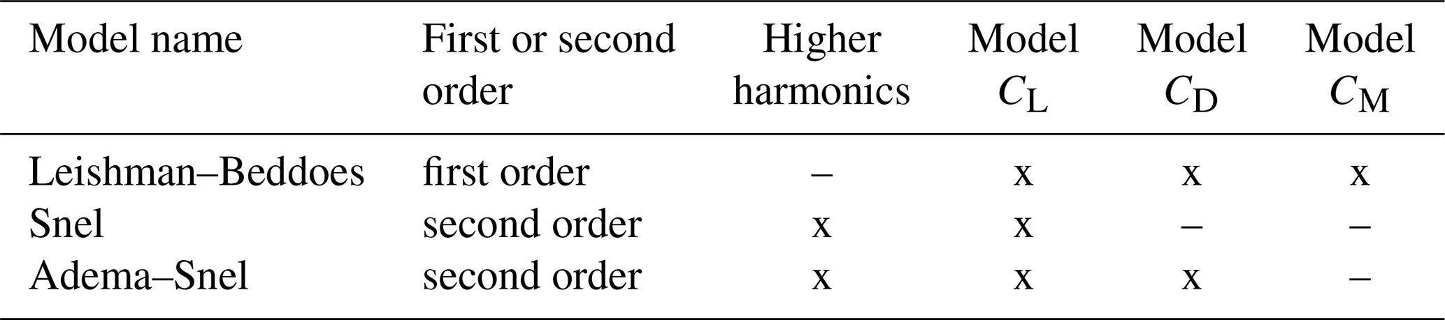
To sum up the characteristics of the above-discussed state-of-the-art dynamic stall models, Table 1 lists the properties of each model and in which aspects the model can be improved further.

Table 1 Properties of the discussed dynamic stall models.

2.4 New second-order IAG model

The proposed IAG model is developed based on knowledge gained from four different models: Leishman–Beddoes, Snel, Adema–Snel and ONERA (Tran and Petot, 1980; Dat and Tran, 1981; Petot, 1989) models with modifications. Similar to the modern models like those from Snel (and ONERA) and its derivatives, the present model is constructed by two main terms: the first-order and second-order corrections. The total dynamic response of the airfoil is formulated as

$$\begin{array}{}\text{(59)}& {\displaystyle }& {\displaystyle }{C}_{{\mathrm{L}}_n}^{\mathrm{D}}=C_{{\mathrm{L}}_n}^{\mathrm{D}\mathrm{1}}+\mathrm{\Delta }{C}_{{\mathrm{L}}_n}^{\mathrm{D}\mathrm{2}},\text{(60)}& {\displaystyle }& {\displaystyle }{C}_{{\mathrm{D}}_n}^{\mathrm{D}}=C_{{\mathrm{D}}_n}^{\mathrm{D}\mathrm{1}}+\mathrm{\Delta }{C}_{{\mathrm{D}}_n}^{\mathrm{D}\mathrm{2}},\text{(61)}& {\displaystyle }& {\displaystyle }{C}_{{\mathrm{M}}_n}^{\mathrm{D}}=C_{{\mathrm{M}}_n}^{\mathrm{D}\mathrm{1}}+\mathrm{\Delta }{C}_{{\mathrm{M}}_n}^{\mathrm{D}\mathrm{2}},\end{array}$$

with ^D1 and ^D2 being the first- and second-order corrections, respectively. Below the description of the modifications made for the new model will be discussed in detail.

2.4.1 First-order correction

Based on the Hopf bifurcation model of Truong (1993) that used the LB model as the starting point of the first-order correction, the present model operates similarly. Despite that, the LB model is not transferred into the state-space formulation, but it is retained as the indical formulation. The model applies the superposition of the solution using a finite-difference approximation to Duhamel's integral to construct the cumulative effect on an arbitrary time history of angle of attack. The LB model described in Sect. 2.1.1 to 2.1.3 will be used with the following modifications.

In the above LB model, predictions for drag are not accurate as will be shown in Sect. 3.1. This inaccuracy lies in the determination of η in Eq. (19) for the tangential force component because drag is more sensitive to tangential force than the lift force is. Also, to maintain simplicity, parameter η is removed, and the tangential force is obtained from the static data at the time-lagged angle of attack ${\mathit{\alpha }}_{{\mathrm{f}}_n}$ by

$$\begin{array}{}\text{(62)}& C_{{\mathrm{T}}_n}^{\mathrm{f}}=C_{\mathrm{T}}^{\mathrm{VISC}}\left({\mathit{\alpha }}_{{\mathrm{f}}_n}\right).\end{array}$$

If one uses this formulation directly, at some point drag still becomes lower than the static drag value by a significant amount. By evaluating the experimental data for several airfoils and various flow conditions, this is not physical at small angles of attack, especially in the downstroke regime, where it usually just returns to the static value. In fact, those experimental data infer that strong drag hysteresis occurs only at high angles of attack beyond stall. Similarly, in the upstroke regime the drag value increases only slightly (approximately only 20 %). In Fig. 3, one can see that drag hysteresis occurs when ζ_n≲ζ_v, with

$$\begin{array}{}\text{(63)}& {\mathit{\zeta }}_n={\displaystyle \frac{\mathrm{1}}{\mathit{\pi }}}{\displaystyle \frac{\mathrm{d}{C}_{\mathrm{N}}}{\mathrm{d}\mathit{\alpha }}}{\left({\displaystyle \frac{\mathrm{1}+\sqrt{f_n}}{\mathrm{2}}}\right)}^{\mathrm{2}},\end{array}$$

and ζ_v is a constant with a value of 0.76. Based on these observations, a simple drag limiting factor is adopted when ζ_n≥0.76 as

$$\begin{array}{}\text{(64)}& C_{{\mathrm{D}}_n}^{\mathrm{D}}=\left\{\begin{array}{l}\mathrm{1.2}{C}_{{\mathrm{D}}_n}^{\mathrm{VISC}};\mathrm{if}{C}_{{\mathrm{D}}_n}^{\mathrm{D}}>\mathrm{1.2}{C}_{{\mathrm{D}}_n}^{\mathrm{VISC}}\\ \mathrm{and}\left(C_{{\mathrm{N}}_n}^{\mathrm{P}}-C_{{\mathrm{N}}_{n-\mathrm{1}}}^{\mathrm{P}}\right)\ge \mathrm{0.0}\\ C_{{\mathrm{D}}_n}^{\mathrm{VISC}};\mathrm{if}\left(C_{{\mathrm{N}}_n}^{\mathrm{P}}-C_{{\mathrm{N}}_{n-\mathrm{1}}}^{\mathrm{P}}\right)<\mathrm{0.0}\\ C_{{\mathrm{D}}_n}^{\mathrm{D}};\mathrm{otherwise}.\end{array}\right.\end{array}$$

Note that for the purpose of numerical implementation, it is always recommended in practice to adopt relaxation to avoid any discontinuity which may present in the above formulation. Furthermore, the value of ζ_v may be chosen differently for different airfoils depending on the vortex lift influence on drag. Further studies on this aspect are encouraged. The effects of these modifications are displayed in Fig. 4.

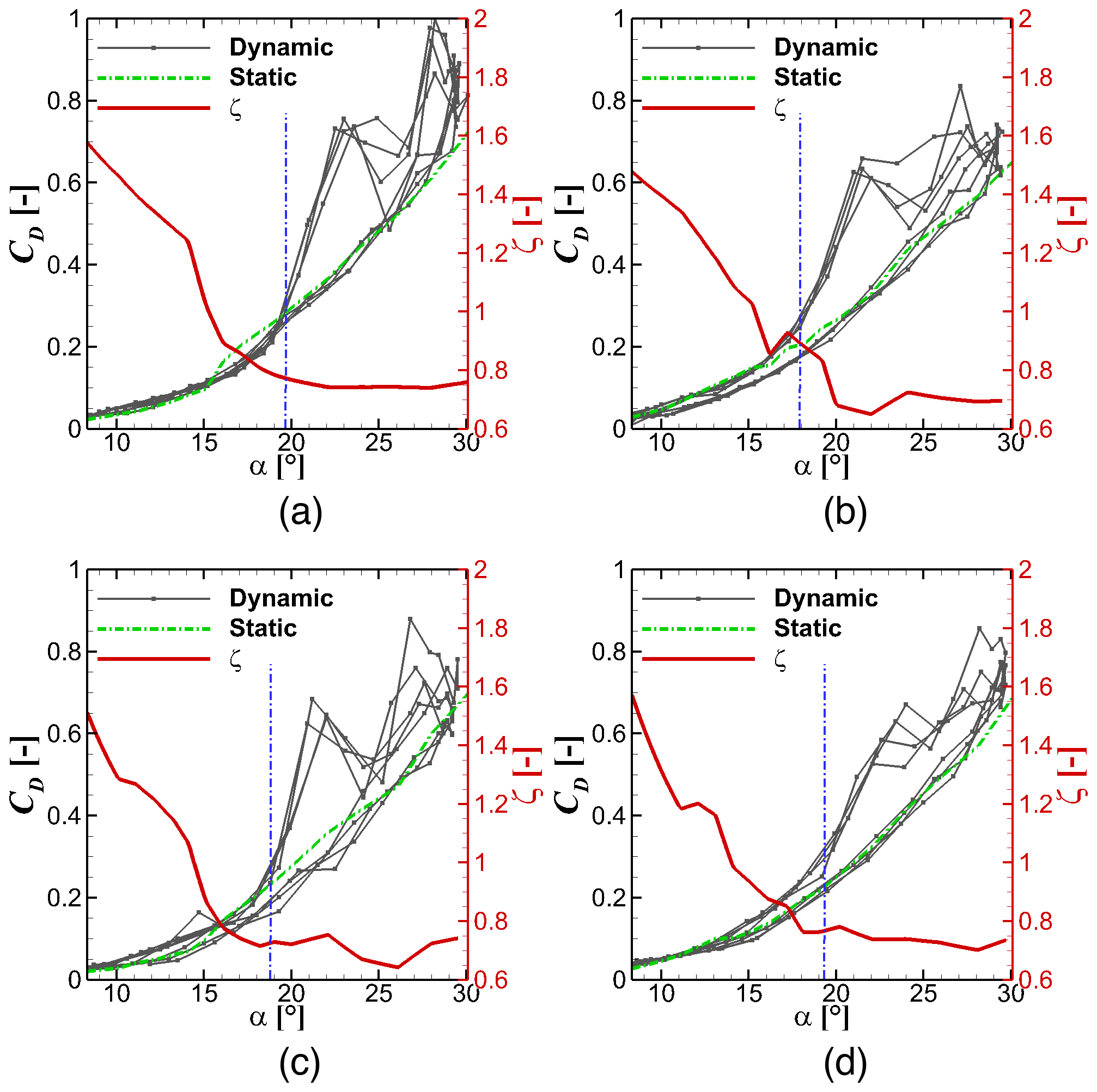
Figure 3 Relation between drag hysteresis in the stall regime with weighted separation parameter ζ for four airfoils. From (a) to (d): S801 (13.5 %), NACA4415 (15 %), S809 (21 %) and S814 (24 %).

It will also be shown in Sect. 3.1 that predicting moment coefficient directly from the static polar data by means of the time-lagged angle of attack has its drawback in the correct damping effect calculation. One may obtain better results by using the “fitting function” as in Eq. (20) instead of using Eq. (34). However, this limits the usability for different airfoils, since the fitting has to be done again for each individual airfoil. For wind turbine simulations, this is fairly impractical because a wind turbine blade is usually constructed by several different airfoils, not to mention the interpolated shapes in between each airfoil position. To solve for this issue, a relatively simple approach is introduced by applying a time delay to the circulatory moment response as

$$\begin{array}{}\text{(65)}& \begin{array}{rl}& C_{{\mathrm{M}}_n}^{\mathrm{C}}=\\ & \left\{\begin{array}{l}{C}_{{\mathrm{M}}_{n-\mathrm{1}}}^{\mathrm{C}}\exp \left(-\frac{\mathrm{\Delta }s}{T_{\mathrm{M}}^{\mathrm{U}}}\right)-C_{\mathrm{P}{f}_n}\left(C_{{\mathrm{V}}_n}-C_{{\mathrm{V}}_{n-\mathrm{1}}}\right)\exp \left(-\frac{\mathrm{\Delta }s}{\mathrm{2}{T}_{\mathrm{M}}^{\mathrm{U}}}\right);\\ \mathrm{if}{\mathit{\tau }}_{{\mathrm{v}}_n}<T_{\mathrm{vl}}\mathrm{and}\mathrm{\Delta }{\mathit{\alpha }}_n\ge \mathrm{0}\\ C_{{\mathrm{M}}_{n-\mathrm{1}}}^{\mathrm{C}}\exp \left(-\frac{\mathrm{\Delta }s}{T_{\mathrm{M}}^{\mathrm{D}}}\right)-C_{\mathrm{P}{f}_n}\left(C_{{\mathrm{V}}_n}-C_{{\mathrm{V}}_{n-\mathrm{1}}}\right)\exp \left(-\frac{\mathrm{\Delta }s}{\mathrm{2}{T}_{\mathrm{M}}^{\mathrm{D}}}\right);\\ \mathrm{if}\mathrm{\Delta }{\mathit{\alpha }}_n<\mathrm{0}\\ C_{{\mathrm{M}}_{n-\mathrm{1}}}^{\mathrm{C}};\mathrm{otherwise}\end{array}\right.\end{array}\end{array}$$

where

$$\begin{array}{}\text{(66)}& C_{\mathrm{P}{f}_n}=K_{\mathrm{f}}^{\mathrm{C}}{\displaystyle \frac{\mathrm{d}{C}_{\mathrm{N}}}{\mathrm{d}\mathit{\alpha }}}\left({\mathit{\alpha }}_n^{\mathrm{CRIT}}-{\mathit{\alpha }}_{\mathrm{0}}^{\mathrm{INV}}\right),\end{array}$$

with $K_{\mathrm{f}}^{\mathrm{C}}$, $T_{\mathrm{M}}^{\mathrm{U}}$ and $T_{\mathrm{M}}^{\mathrm{D}}$ being constants relatively insensitive to airfoils. Furthermore, the second condition of Eq. (35) is modified to avoid discontinuity which occurs at a large reduced frequency (e.g., k=0.2) for any LB-based models without recalibration of the time constant as

$$\begin{array}{}\text{(67)}& {\mathit{\tau }}_{{\mathrm{v}}_n}=\left\{\begin{array}{ll}{\mathit{\tau }}_{{\mathrm{v}}_{n-\mathrm{1}}}+\mathrm{0.45}\frac{\mathrm{\Delta }t}{c}V;& \mathrm{if}{C}_{{\mathrm{N}}_n}^{\mathrm{P}\mathrm{1}}>C_{\mathrm{N}}^{\mathrm{CRIT}}\\ {\mathit{\tau }}_{{\mathrm{v}}_{n-\mathrm{1}}}\exp (-\mathrm{\Delta }s);& \mathrm{if}{C}_{{\mathrm{N}}_n}^{\mathrm{P}\mathrm{1}}<C_{\mathrm{N}}\mathrm{CRIT}\mathrm{and}\mathrm{\Delta }{\mathit{\alpha }}_n\ge \mathrm{0}\\ {\mathit{\tau }}_{{\mathrm{v}}_{n-\mathrm{1}}};& \mathrm{otherwise}.\end{array}\right.\end{array}$$

The effects of these modifications are displayed in Fig. 5.

Figure 4 Drag reconstruction in comparison with the experimental data for the S801 airfoil (Ramsay et al., 1996) applying (a) Eq. (19), (b) Eq. (62), and (c) Eqs. (62) and (64).

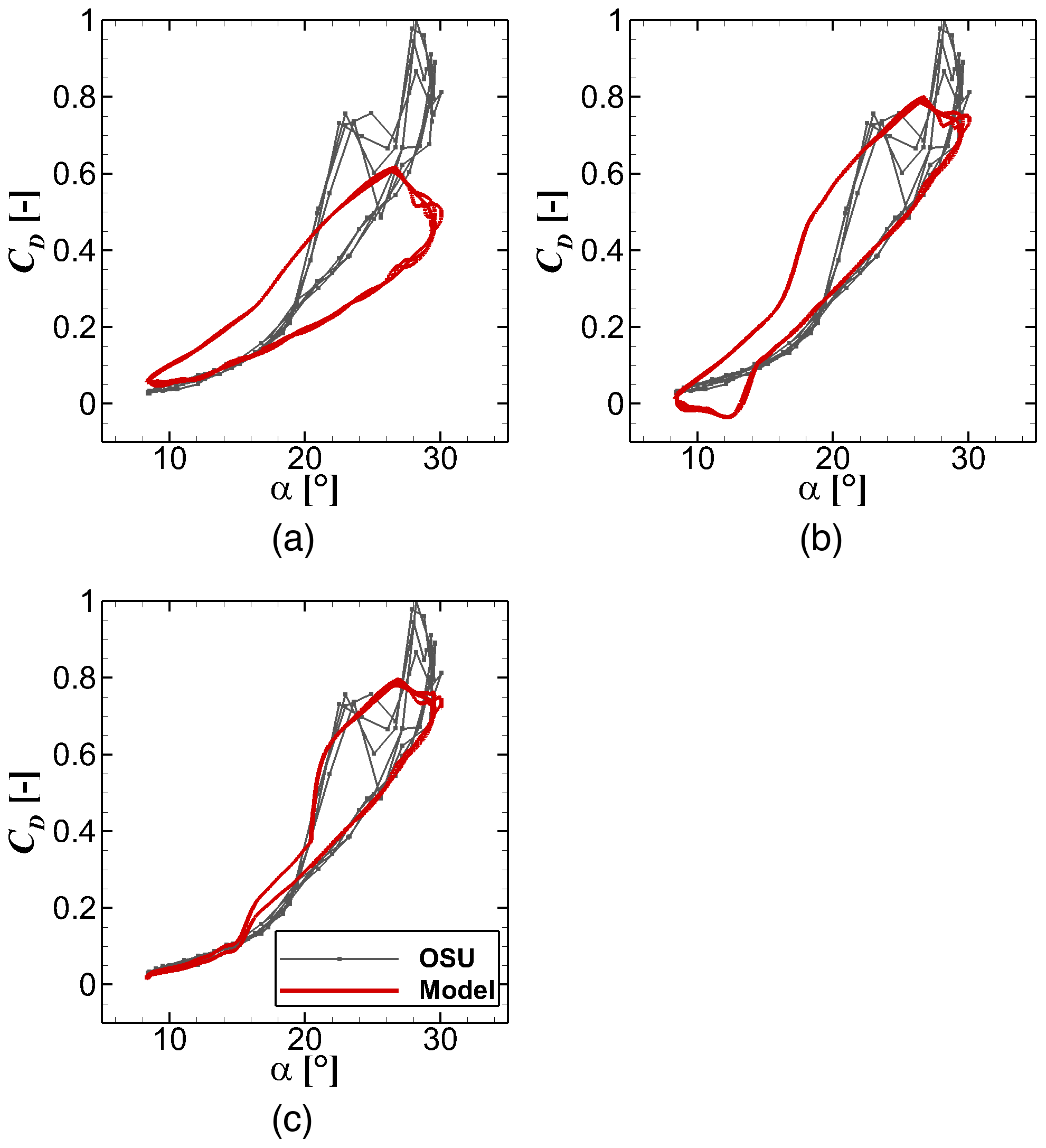
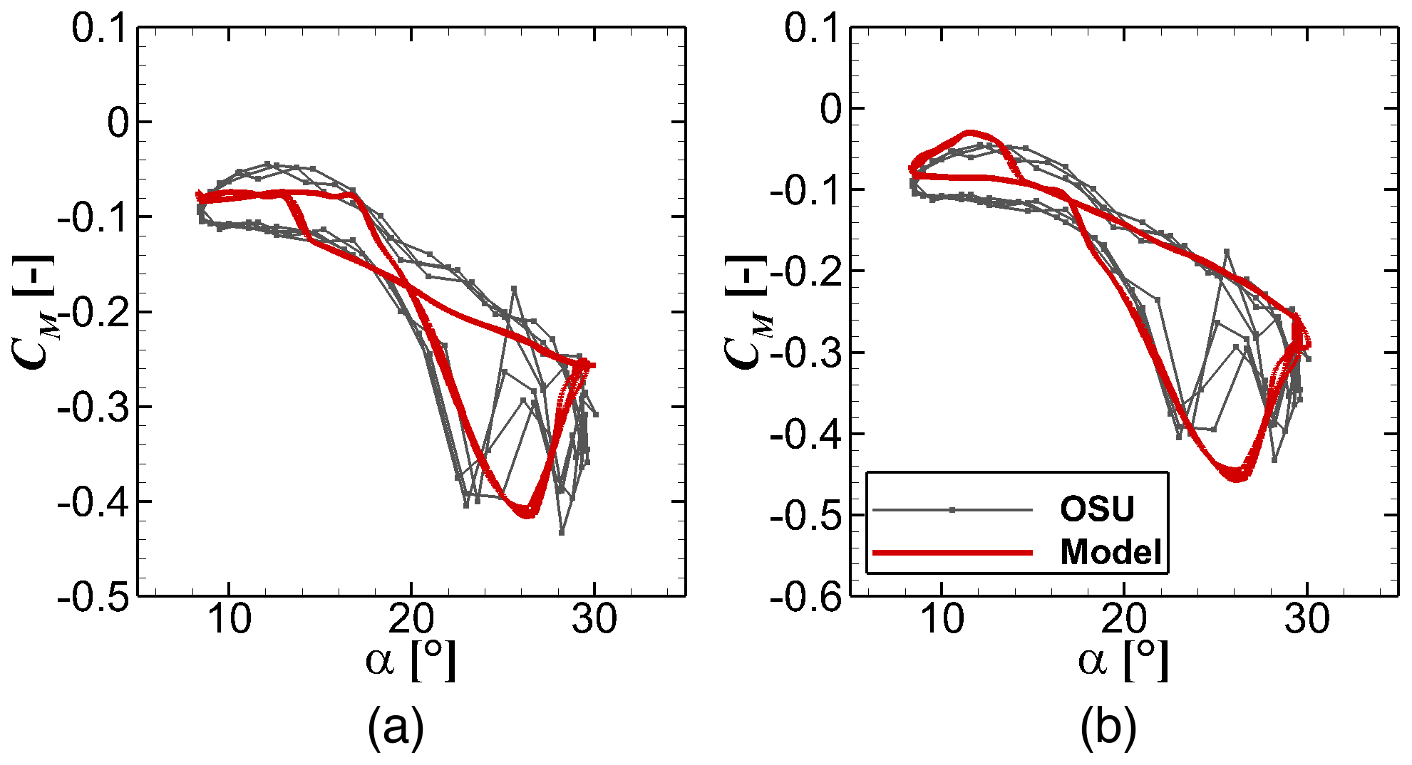
Figure 5 Moment reconstruction in comparison with the experimental data for the S801 airfoil (Ramsay et al., 1996) applying (a) Eq. (34) and (b) Eq. (65).

The total first-order dynamic response of the airfoil is formulated as

$$\begin{array}{}\text{(68)}& {\displaystyle }& {\displaystyle }{C}_{{\mathrm{N}}_n}^{\mathrm{D}\mathrm{1}}=C_{{\mathrm{N}}_n}^{\mathrm{f}}+C_{{\mathrm{N}}_n}^{\mathrm{V}},\text{(69)}& {\displaystyle }& {\displaystyle }{C}_{{\mathrm{T}}_n}^{\mathrm{D}\mathrm{1}}=C_{{\mathrm{T}}_n}^{\mathrm{f}},\text{(70)}& {\displaystyle }& {\displaystyle }{C}_{{\mathrm{M}}_n}^{\mathrm{D}\mathrm{1}}=C_{{\mathrm{M}}_n}^{\mathrm{f}}+C_{{\mathrm{M}}_n}^{\mathrm{V}}+C_{{\mathrm{M}}_n}^{\mathrm{C}},\end{array}$$

where the definition and description of each variable were given in Sect. 2.1 for the LB model. Thus the first-order lift and drag responses can be obtained by

$$\begin{array}{}\text{(71)}& {\displaystyle }& {\displaystyle }{C}_{{\mathrm{L}}_n}^{\mathrm{D}\mathrm{1}}=C_{{\mathrm{N}}_n}^{\mathrm{D}\mathrm{1}}\cos {\mathit{\alpha }}_n-C_{{\mathrm{T}}_n}^{\mathrm{D}\mathrm{1}}\sin {\mathit{\alpha }}_n,\text{(72)}& {\displaystyle }& {\displaystyle }{C}_{{\mathrm{D}}_n}^{\mathrm{D}\mathrm{1}}=C_{{\mathrm{N}}_n}^{\mathrm{D}\mathrm{1}}\sin {\mathit{\alpha }}_n+C_{{\mathrm{T}}_n}^{\mathrm{D}\mathrm{1}}\cos {\mathit{\alpha }}_n.\end{array}$$

2.4.2 Second-order correction

The second-order correction takes the form of the non-linear ordinary differential equation according to the second-order correction of the Snel (Snel, 1997) and Adema–Snel (Adema et al., 2020) models. Generally, the basis of implementation of the present model mostly uses the Adema–Snel (Adema et al., 2020) model where the normal force is used instead of the lift force as for the original Snel model (Snel, 1997) as

$$\begin{array}{}\text{(73)}& {\ddot{\mathrm{\Delta }C}}_{{\mathrm{N}}_n}^{\mathrm{D}\mathrm{2}}+K{f}_{{\mathrm{21}}_n}{\dot{\mathrm{\Delta }C}}_{{\mathrm{N}}_n}^{\mathrm{D}\mathrm{2}}+K{f}_{{\mathrm{20}}_n}\mathrm{\Delta }{C}_{{\mathrm{N}}_n}^{\mathrm{D}\mathrm{2}}=F_{{\mathrm{2}}_n}.\end{array}$$

This way, shedding effects apply not only to the lift force but also to the drag force. Note that τ is not present in Eq. (73) in contrast to the original formulation in Eqs. (44) and (55). The equation is changed because the time derivatives in the above equation are no longer with respect to time but to $s=\mathrm{2}Vt/c$, similar to the ONERA model (Tran and Petot, 1980; Dat and Tran, 1981; Petot, 1989). This is done to nondimensionalize the equations.

In Eq. (57), the k_s was projected as a function of the angle of attack by sin α_n. This modification causes problems when the hysteresis effect takes place in both positive and negative angles because Eq. (57) will be zero and then negative, causing instability of the ODE. Thus, the original form of the Snel model (Snel, 1997) is retained in the present model, but the constant is modified as

$$\begin{array}{}\text{(74)}& K{f}_{{\mathrm{20}}_n}=\mathrm{20}{k}_{\mathrm{s}}^{\mathrm{2}}\left[\mathrm{1}+\mathrm{3}{\left(\mathrm{\Delta }{C}_{{\mathrm{N}}_n}^{\mathrm{D}\mathrm{2}}\right)}^{\mathrm{2}}\right]\left[\mathrm{1}+\mathrm{3}{\dot{{\mathit{\alpha }}_n}}^{\mathrm{2}}\right].\end{array}$$

The idea for the downstroke damping as in Eq. (58) is adopted in the present model; the following form and constants are used:

$$\begin{array}{}\text{(75)}& K{f}_{{\mathrm{21}}_n}=\left\{\begin{array}{l}\mathrm{150}{k}_{\mathrm{s}}\left[-\mathrm{0.01}\left(\mathrm{\Delta }{C}_{{\mathrm{N}}_n}^{\mathrm{INV}}-\mathrm{0.5}\right)+\mathrm{2}{\left(\mathrm{\Delta }{C}_{{\mathrm{N}}_n}^{\mathrm{D}\mathrm{2}}\right)}^{\mathrm{2}}\right];\\ \mathrm{if}\dot{{\mathit{\alpha }}_n}>\mathrm{0}\\ \mathrm{30}{k}_{\mathrm{s}}\left[-\mathrm{0.01}\left(\mathrm{\Delta }{C}_{{\mathrm{N}}_n}^{\mathrm{INV}}-\mathrm{0.5}\right)+\mathrm{14}{\left(\mathrm{\Delta }{C}_{{\mathrm{N}}_n}^{\mathrm{D}\mathrm{2}}\right)}^{\mathrm{2}}\right];\\ \mathrm{if}\dot{{\mathit{\alpha }}_n}\le \mathrm{0}\mathrm{and}{\mathit{\alpha }}_n\ge {\mathit{\alpha }}_n^{\mathrm{CRIT}}\\ \mathrm{0.2}{k}_{\mathrm{s}};\\ \mathrm{if}\dot{{\mathit{\alpha }}_n}\le \mathrm{0}\mathrm{and}{\mathit{\alpha }}_n<{\mathit{\alpha }}_n^{\mathrm{CRIT}}.\end{array}\right.\end{array}$$

Note again that τ is not present in the above equation. The original formulation in Eq. (58) replaces the damped oscillator when $\dot{{\mathit{\alpha }}_n}\le \mathrm{0}$ for a self-excited oscillator of Van der Pol type with more damping. This is in contrast with the implementation done in Truong (2016), where the self-excited oscillator is only replaced by the damped oscillator, when the flow is reattached on the return cycle. Under such circumstances, the oscillatory behavior still subsists in the return cycle, albeit with smaller amplitude. To accommodate this aspect, the last term of Eq. (75) is applied when the angle is smaller than ${\mathit{\alpha }}_n^{\mathrm{CRIT}}$. As for the forcing term, the original form of the Snel model (Snel, 1997) is adopted as

$$\begin{array}{}\text{(76)}& F_{{\mathrm{2}}_n}=\mathrm{0.5}{k}_{\mathrm{s}}\left(-\mathrm{0.15}\mathrm{\Delta }{C}_{{\mathrm{N}}_n}^{\mathrm{INV}}+\mathrm{0.05}{\dot{\mathrm{\Delta }C}}_{{\mathrm{N}}_n}^{\mathrm{INV}}\right).\end{array}$$

To facilitate the inclusion of the higher harmonic effects for the pitching moment, the idealized center of pressure obtained in the first-order correction given in Eq. (26) is passed into the second-order model. Thus, the dynamic moment reaction takes the form

$$\begin{array}{}\text{(77)}& \mathrm{\Delta }{C}_{{\mathrm{M}}_n}^{\mathrm{D}\mathrm{2}}=-C_{{\mathrm{Pv}}_n}\mathrm{\Delta }{C}_{{\mathrm{N}}_n}^{\mathrm{D}\mathrm{2}}.\end{array}$$

Regarding the tangential force, a similar assumption is made as in Eq. (49) where the influence of $\mathrm{\Delta }{C}_{{\mathrm{T}}_n}^{\mathrm{D}\mathrm{2}}$ is neglected in the formulation, but $\mathrm{\Delta }{C}_{{\mathrm{T}}_n}^{\mathrm{D}\mathrm{1}}$ is considered in the first-order term correction described above. Finally, the second-order term of the lift ($\mathrm{\Delta }{C}_{{\mathrm{L}}_n}^{\mathrm{D}\mathrm{2}}$) and drag ($\mathrm{\Delta }{C}_{{\mathrm{D}}_n}^{\mathrm{D}\mathrm{2}}$) can be calculated easily. The effects of the second-order term are displayed in Fig. 6.

Figure 6 Airfoil response reconstruction in comparison with the experimental data for the S801 airfoil (Ramsay et al., 1996) applying only the first-order correction and with inclusion of the second-order term. (a) Lift, (b) drag and (c) pitching moment.

2.5 Constants applied for the investigated dynamic stall models

The following constants are applied in the implemented dynamic stall models. These values are kept constant throughout the paper. The constants for the Leishman–Beddoes model and for the proposed IAG model are given in Tables 2 and 3, respectively. For any model developed based on the Leishman–Beddoes type, the critical angle of attack plays a major role. This can be obtained as the angle where the viscous pitching moment breaks or when the drag increases significantly (or the stall angle). The applied critical angles are given in Table 4. The validation is done by comparing the calculations with experimental data obtained at The Ohio State University for the S801 airfoil (13.5 % relative thickness) (Ramsay et al., 1996), NACA4415 airfoil (15 % relative thickness) (Hoffman et al., 1996), S809 airfoil (21 % relative thickness) (Ramsay et al., 1995) and S814 airfoil (24 % relative thickness) (Janiszewska et al., 1996). All selected test cases for the airfoils are employed with a leading edge grit (turbulator) to enable the “soiled” effects on a wind turbine blade at a Reynolds number of around 750 K. Note that these polar data are different from those used for example by Sheng et al. (2010) where the natural transition cases were taken. Therefore, the critical angles of attack are also different. The results of the studies are presented in the following sections.

Table 2 Constants applied for the Leishman–Beddoes model.

Table 3 Constants applied for the IAG model.

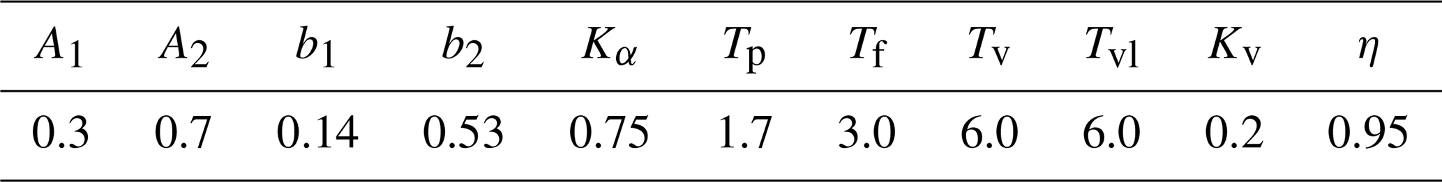
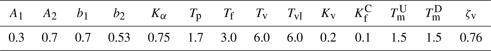
Table 4 Critical angle of attack (${\mathit{\alpha }}_n^{\mathrm{CRIT}}$) applied for the Leishman–Beddoes and IAG models.

3 Results and discussion

The three state-of-the-art dynamic stall models reviewed above (Leishman–Beddoes, Snel, Adema–Snel) have been used as a basis for examining the dynamic loads of four different pitching airfoils at various flow conditions. Experience gained from those models is used to formulate a new second-order dynamic stall model, namely the IAG model, by evaluating the weakness and strength of each model. The presented second-order models need to solve a set of differential equations. For this purpose, the Euler–Heun forward integration method is used.

3.1 Comparison against experimental data

This section compares the predicted dynamic forces and the measurement data. For a fair comparison, all models are assessed with the same time step size of $\mathrm{\Delta }t=T/\mathrm{1440}$, with T being the pitching period. The evaluations are performed on the S801 airfoil at k=0.073. The comparison of each model is shown in Figs. 7 to 9 for the Snel, Adema and IAG models, respectively. Note that the constants of the other existing dynamic stall models are taken directly from literature without further calibration for the S801 airfoil. Therefore, it is already expected that their performance will not be optimal. The main purpose of the comparison is not to study their accuracy but to analyze the robustness of each model for a different airfoil without tuning the constants. On the other hand, the constants for the IAG model in Table 3 were obtained using the S801 airfoil. To enable a fair assessment of the model robustness, the IAG model will also be used to reconstruct the dynamic polar data of four airfoils with different relative thicknesses without changing the constants in Sect. 3.6.

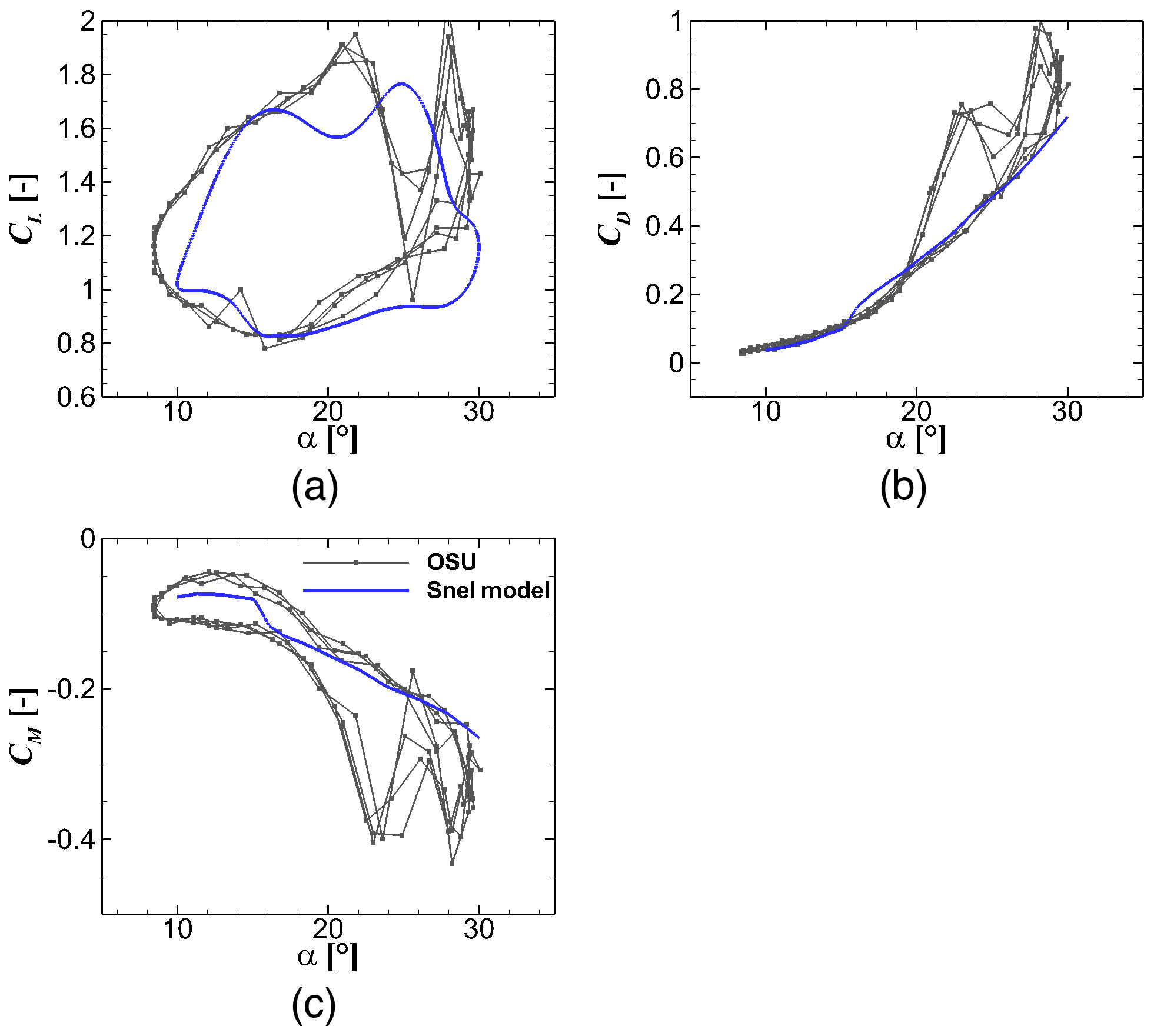
Figure 7 Dynamic force reconstruction using the Snel model in comparison with the measurement data (Ramsay et al., 1996) for $\mathrm{\Delta }t=T/\mathrm{1440}$. S801 airfoil, k=0.073, $\stackrel{\mathrm{‾}}{\mathit{\alpha }}=\mathrm{20}{}^{\circ }$ and $\mathrm{\Delta }\mathit{\alpha }=\mathrm{10}{}^{\circ }$.

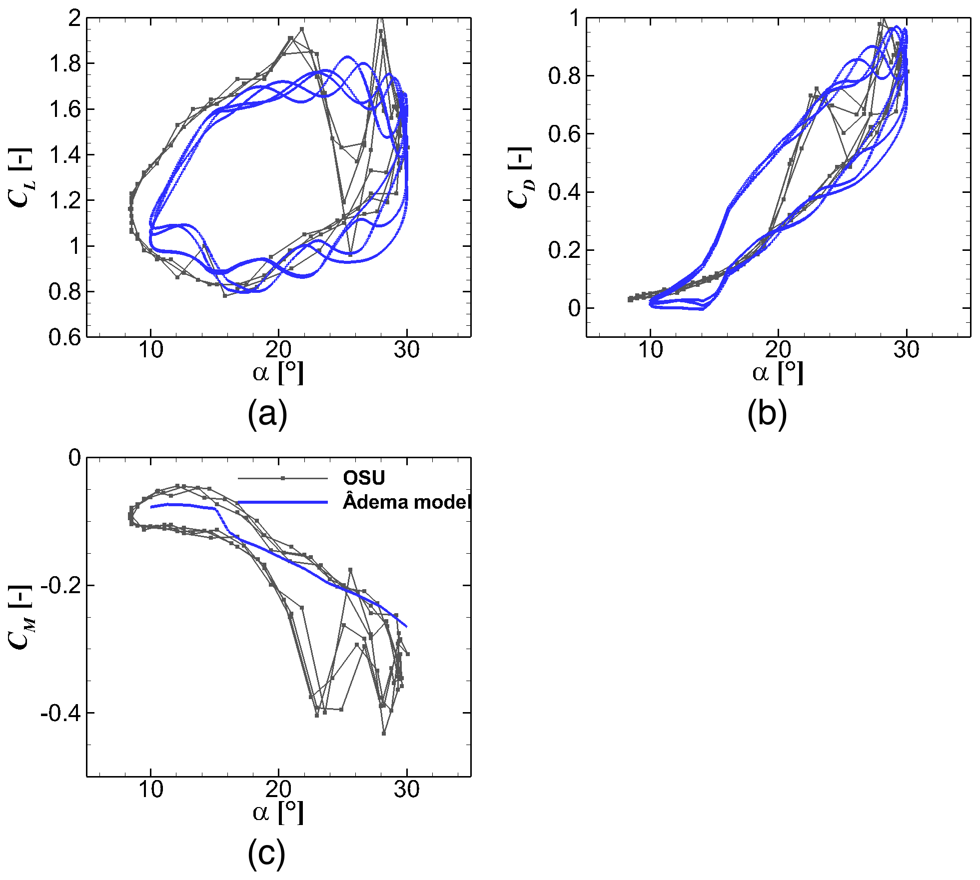
Figure 8 Dynamic force reconstruction using the Adema model in comparison with the measurement data (Ramsay et al., 1996) for $\mathrm{\Delta }t=T/\mathrm{1440}$. S801 airfoil, k=0.073, $\stackrel{\mathrm{‾}}{\mathit{\alpha }}=\mathrm{20}{}^{\circ }$ and $\mathrm{\Delta }\mathit{\alpha }=\mathrm{10}{}^{\circ }$.

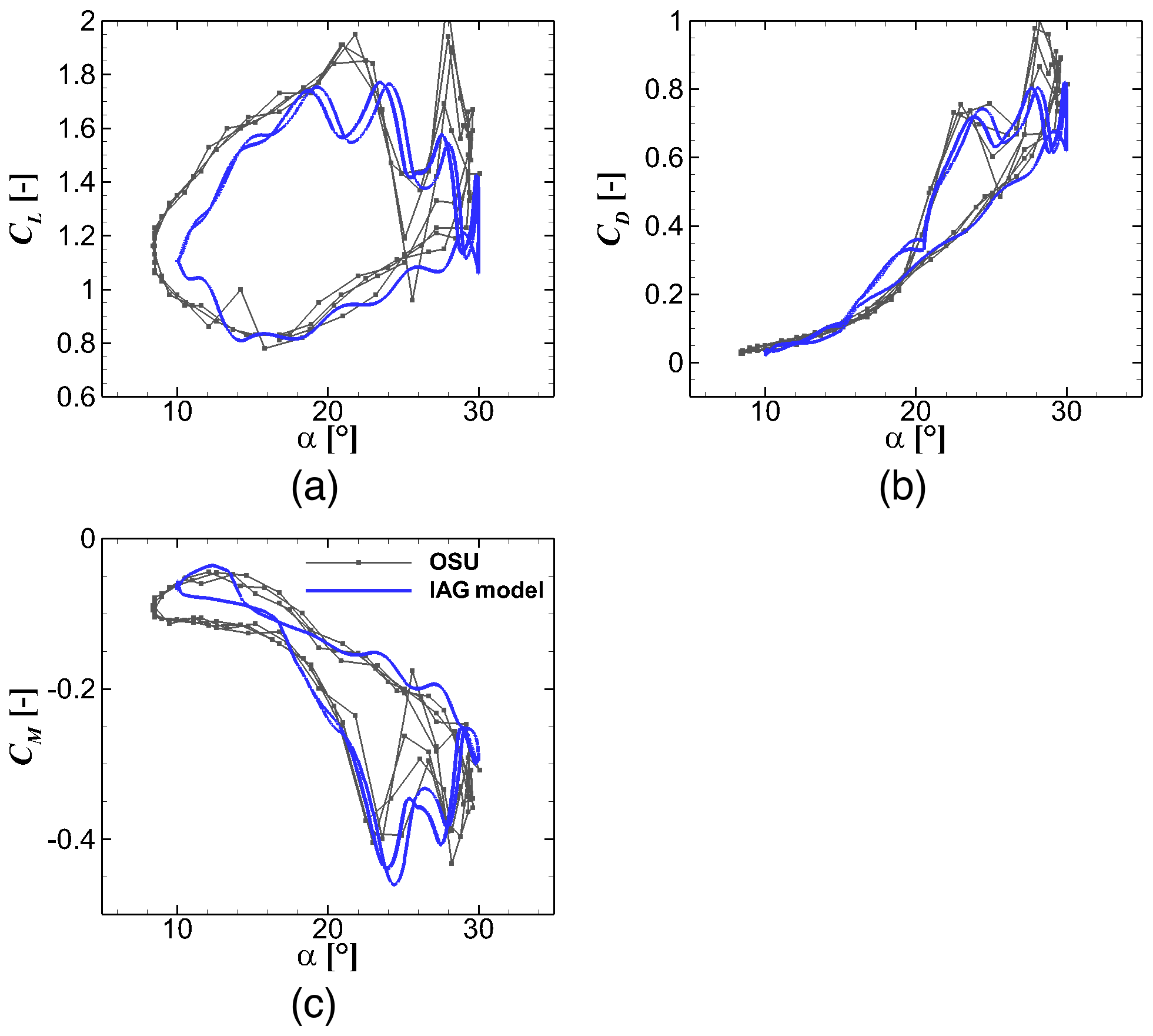
Figure 9 Dynamic force reconstruction using the IAG model in comparison with the measurement data (Ramsay et al., 1996) for $\mathrm{\Delta }t=T/\mathrm{1440}$. S801 airfoil, k=0.073, $\stackrel{\mathrm{‾}}{\mathit{\alpha }}=\mathrm{20}{}^{\circ }$ and $\mathrm{\Delta }\mathit{\alpha }=\mathrm{10}{}^{\circ }$.

The original Snel models cannot predict the drag and moment coefficients in the original formulations. Thus, only the static polar data are shown. The Snel model actually shows an acceptable accuracy even though the constants are taken as found in literature. The higher harmonic effects are unfortunately not captured by this model. This is further refined by the Adema model which was developed as an improvement for the Snel model. The model performs fairly well for the lift and drag predictions, though the drag value at small angles of attack is a bit off. The pitching moment prediction is also not included in its formulations. These disadvantages are better treated in the proposed IAG model. Not only the prediction of the lift coefficient but also the accuracy of drag prediction are improved significantly. The modifications described in Sect. 2.4 result in the improvement at low and high angle-of-attack regimes. The model is also able to reconstruct the pitching moment polar accurately, which is important for aeroelastic calculations of wind turbine blades.

For the following sections, the proposed IAG model will be tested under various flow conditions and for several airfoils at various relative thicknesses in comparison with measurement data. Note that these calculations are performed without changing the constants to assess the robustness of the model at different flow conditions.

3.2 Effects of time signal deviation

The actual pitching motion within The Ohio State University (OSU) measurement differs slightly from the intended motion. The actual time series of the angle of attack is included in the experimental data (Ramsay et al., 1996; Hoffman et al., 1996; Ramsay et al., 1995; Janiszewska et al., 1996). To assess the effects of this time signal deviation on the aerodynamic response, the calculations using these time signal data were performed applying the IAG model. The results are compared with the experimental data and the results of the IAG model presented in Sect. 3.1. Note that these time signal data are fairly coarse and can cause problems for second-order dynamic stall models because the gradient of α change can be extremely large. To cover for this issue, the time signal is interpolated in between each available point using a third-order cubic-spline interpolation. The time signals are discretized by $\mathrm{\Delta }t=T/\mathrm{1440}$ over a single pitching period. The first period of oscillation is used for initialization of the time integration; thus a constant angle of attack is applied as shown in Fig. 10.

Figure 10 Comparison of the time series of the idealized sinusoidal angle of attack to the exact signals in the experimental campaign for the S801 airfoil, k=0.073, $\stackrel{\mathrm{‾}}{\mathit{\alpha }}=\mathrm{20}{}^{\circ }$ and $\mathrm{\Delta }\mathit{\alpha }=\mathrm{10}{}^{\circ }$.

Figure 11 presents the influence of the time signal variation on the aerodynamic performance in terms of C_L, C_D and C_M. TS labels the exact time signals in the experimental campaign. Although the time signal difference has almost no influence on the global prediction characteristics, some deviation from the idealized sinusoidal motion can be noticed clearly. For example, one can see the increased lift buildup in the upstroke regime before stall and the location of the lift stall. Some deviations in the drag and pitching moment coefficients are observed as well. For the rest of the paper, the prediction procedure using the actual time signal from the experimental data is used for the best consistency with the experimental campaign.

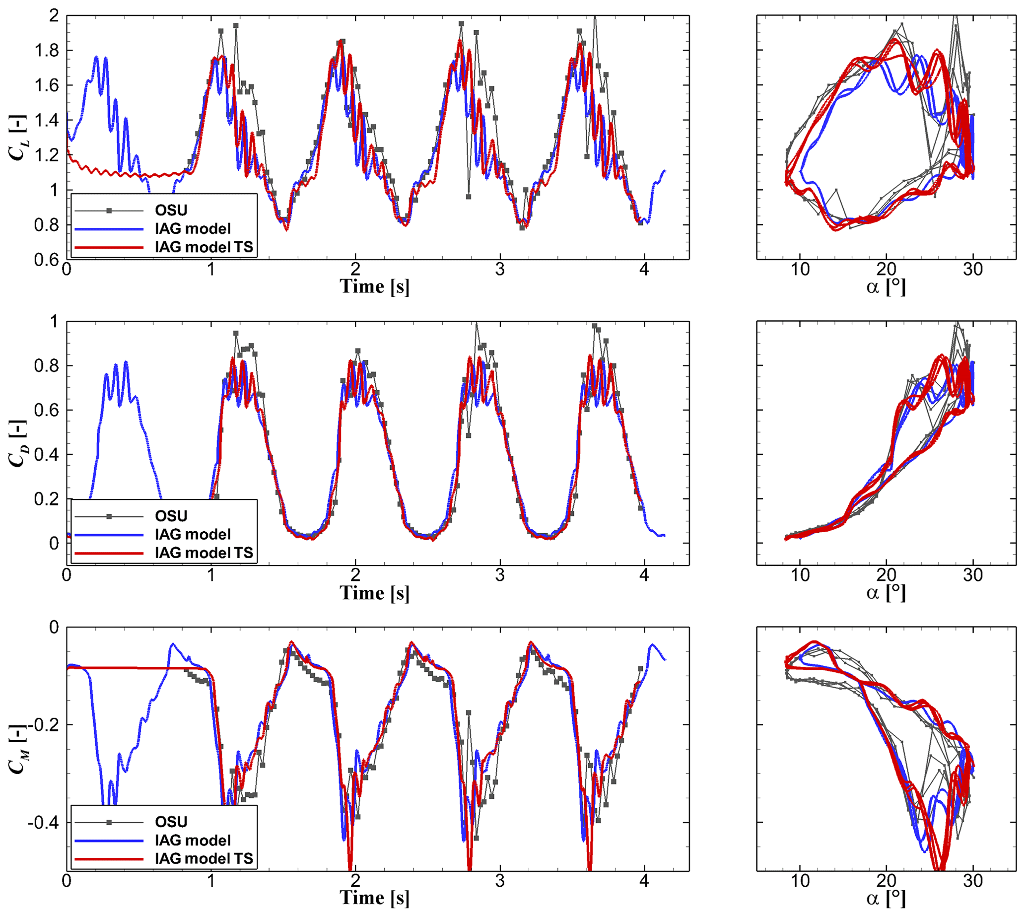
Figure 11 Dynamic force reconstruction by the IAG model in comparison with the measurement data (Ramsay et al., 1996) for $\mathrm{\Delta }t=T/\mathrm{1440}$ using the actual angle of attack in the experimental campaign. TS labels the exact time signals in the experimental campaign. S801 airfoil, k=0.073, $\stackrel{\mathrm{‾}}{\mathit{\alpha }}=\mathrm{20}{}^{\circ }$ and $\mathrm{\Delta }\mathit{\alpha }=\mathrm{10}{}^{\circ }$.

3.3 Performance of the model for different mean angles of incidence

In this section, the effects of the mean angle of attack are evaluated. Three different angles of attack at the same inflow conditions are selected for this purpose. These are $\stackrel{\mathrm{‾}}{\mathit{\alpha }}=\mathrm{8}$, 14 and 20^∘. Note that these mean angles of attack are only approximations since the actual time signal data from the experimental campaign are used. The selected mean angles represent the regime of attached flow, partly separated flow and fully separated flow conditions. These are helpful to assess the model performance under various flow situations.

Figure 12 presents the results for the lift coefficient under these three investigated mean angles of attack. The model performs very well for these different cases. The maximum lift is a bit overestimated in the model for the lowest $\stackrel{\mathrm{‾}}{\mathit{\alpha }}$, but in general all unsteady lift characteristics in the measurement data are reproduced in a sound agreement with the experimental data. A similar behavior is shown for the drag prediction depicted in Fig. 13. The proposed model captures the increased drag effect and its shedding characteristics well. The simple modifications applied in Sect. 2.4 result in a good prediction of the drag coefficient compared with the experimental data. In Fig. 14, the prediction for pitching moment is shown. Here the predicted moment coefficient is in a good agreement with the measured values.

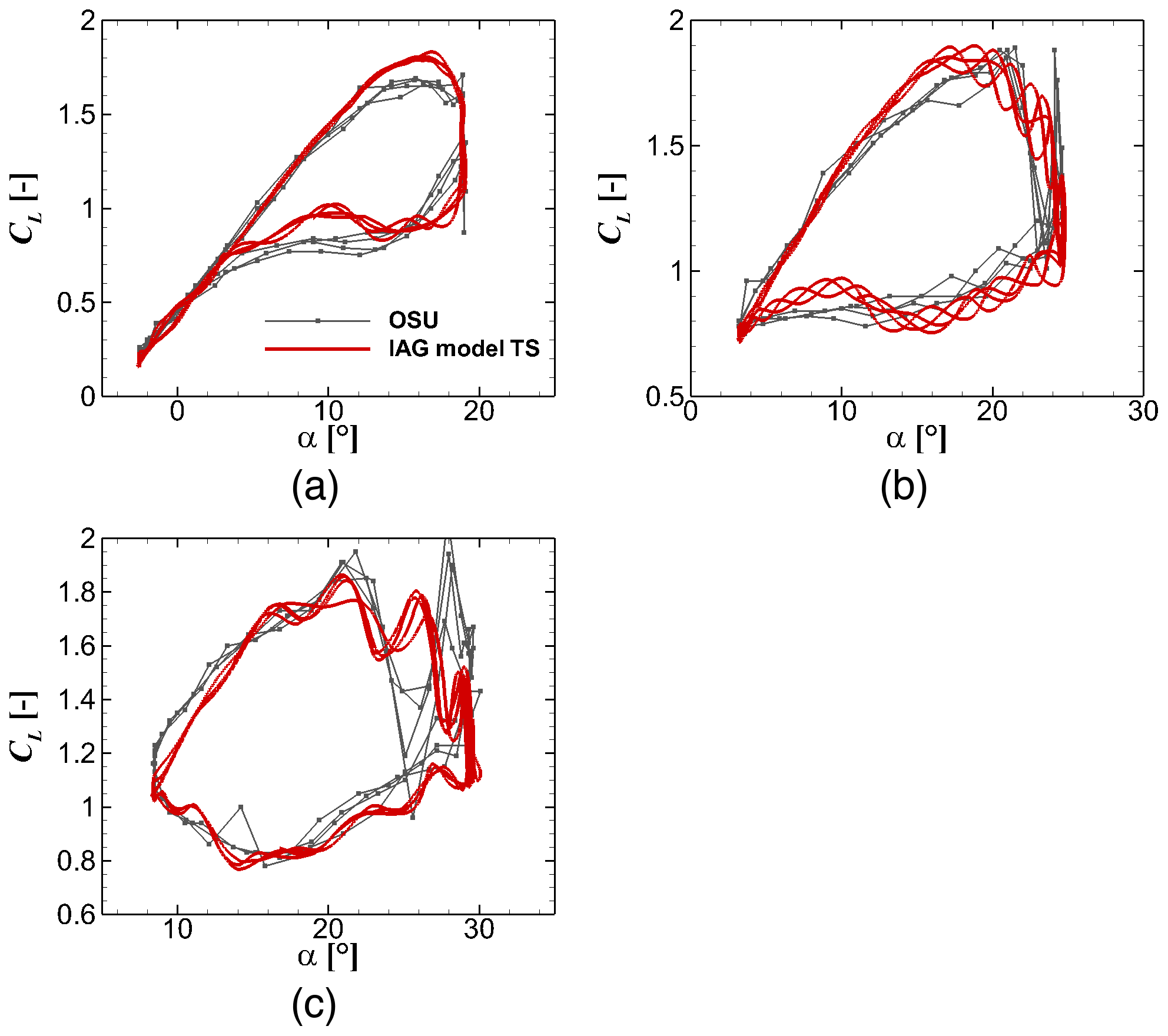
Figure 12 Lift reconstruction by the IAG model in comparison with the measurement data (Ramsay et al., 1996) for $\mathrm{\Delta }t=T/\mathrm{1440}$ using the actual angle of attack in the experimental campaign at various $\stackrel{\mathrm{‾}}{\mathit{\alpha }}$ values. From (a) to (c): $\stackrel{\mathrm{‾}}{\mathit{\alpha }}=\mathrm{8}$, $\stackrel{\mathrm{‾}}{\mathit{\alpha }}=\mathrm{14}$ and $\stackrel{\mathrm{‾}}{\mathit{\alpha }}=\mathrm{20}{}^{\circ }$. S801 airfoil, k=0.073 and $\mathrm{\Delta }\mathit{\alpha }=\mathrm{10}{}^{\circ }$.

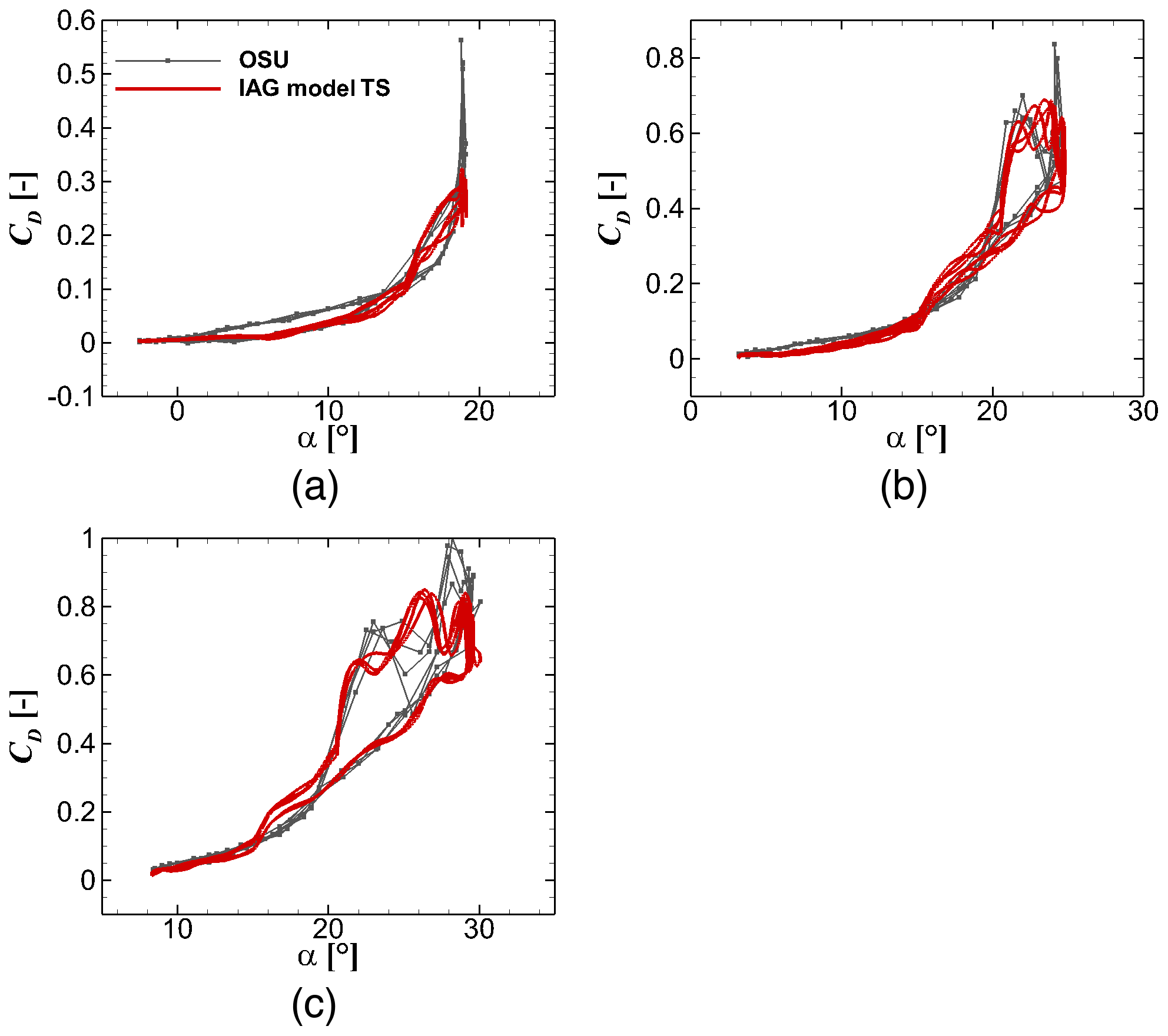
Figure 13 Drag reconstruction by the IAG model in comparison with the measurement data (Ramsay et al., 1996) for $\mathrm{\Delta }t=T/\mathrm{1440}$ using the actual angle of attack in the experimental campaign at various $\stackrel{\mathrm{‾}}{\mathit{\alpha }}$ values. From (a) to (c): $\stackrel{\mathrm{‾}}{\mathit{\alpha }}=\mathrm{8}$, $\stackrel{\mathrm{‾}}{\mathit{\alpha }}=\mathrm{14}$ and $\stackrel{\mathrm{‾}}{\mathit{\alpha }}=\mathrm{20}{}^{\circ }$. S801 airfoil, k=0.073 and $\mathrm{\Delta }\mathit{\alpha }=\mathrm{10}{}^{\circ }$.

Figure 14 Pitching moment reconstruction by the IAG model in comparison with the measurement data (Ramsay et al., 1996) for $\mathrm{\Delta }t=T/\mathrm{1440}$ using the actual angle of attack in the experimental campaign at various $\stackrel{\mathrm{‾}}{\mathit{\alpha }}$ values. From (a) to (c): $\stackrel{\mathrm{‾}}{\mathit{\alpha }}=\mathrm{8}$, $\stackrel{\mathrm{‾}}{\mathit{\alpha }}=\mathrm{14}$ and $\stackrel{\mathrm{‾}}{\mathit{\alpha }}=\mathrm{20}{}^{\circ }$. S801 airfoil, k=0.073 and $\mathrm{\Delta }\mathit{\alpha }=\mathrm{10}{}^{\circ }$.

3.4 Performance of the model for different reduced frequencies

The effects of pitching frequency on the aerodynamic response will be discussed in this section. Three different reduced frequencies are examined, namely k=0.036, 0.073 and 0.111. The stall regime is shown here, where the prediction is the most challenging. The actual time signals as of the measurement campaign are used, following the procedure described in Sect. 3.2.

Figure 15 displays the results for the dynamic lift coefficient response. The lowest reduced frequency of 0.036 is dominated by the viscous effects. It represents the case where the “delayed” angle-of-attack response is the weakest. It can be seen that the maximum attained lift coefficient increases with increasing k. The gradient of the lift polar in the upstroke and downstroke phases also increases as well. These characteristics are present in both experimental data and predictions delivered by the IAG model. A similar behavior is also displayed in drag and pitching moments in Figs. 16 and 17, respectively. It is obvious that stall occurs much earlier for a smaller k value. One can see that the maximum amplitude of all three force components increases with increasing k. This can be dangerous for the structural stability, since the amplitude determines the fatigue loads.

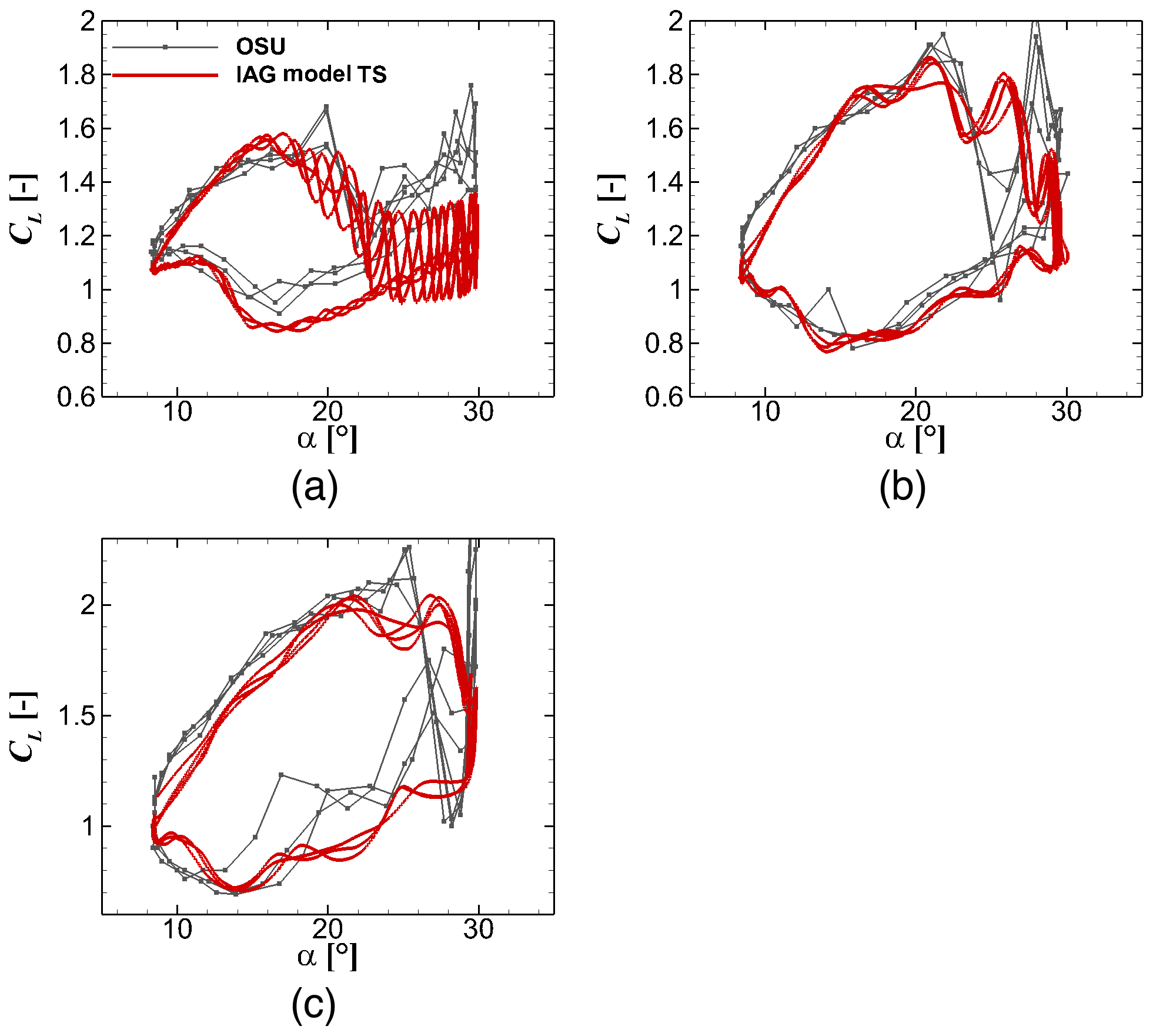
Figure 15 Lift reconstruction by the IAG model in comparison with the measurement data (Ramsay et al., 1996) for $\mathrm{\Delta }t=T/\mathrm{1440}$ using the actual angle of attack in the experimental campaign at various k values. From (a) to (c): k=0.036, k=0.073 and k=0.111. S801 airfoil, $\stackrel{\mathrm{‾}}{\mathit{\alpha }}=\mathrm{20}$ and $\mathrm{\Delta }\mathit{\alpha }=\mathrm{10}{}^{\circ }$.

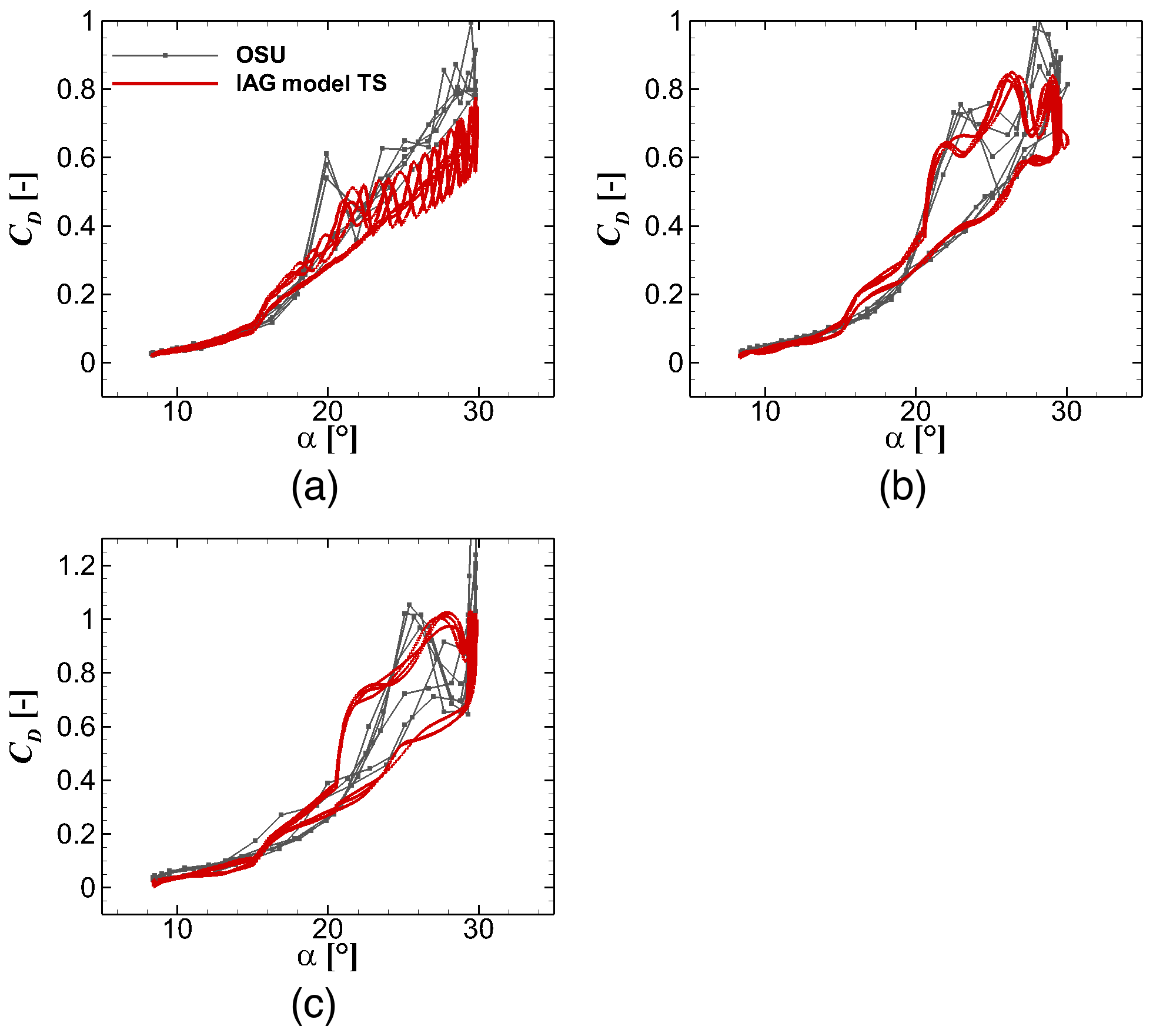
Figure 16 Drag reconstruction by the IAG model in comparison with the measurement data (Ramsay et al., 1996) for $\mathrm{\Delta }t=T/\mathrm{1440}$ using the actual angle of attack in the experimental campaign at various k values. From (a) to (c): k=0.036, k=0.073 and k=0.111. S801 airfoil, $\stackrel{\mathrm{‾}}{\mathit{\alpha }}=\mathrm{20}$ and $\mathrm{\Delta }\mathit{\alpha }=\mathrm{10}{}^{\circ }$.

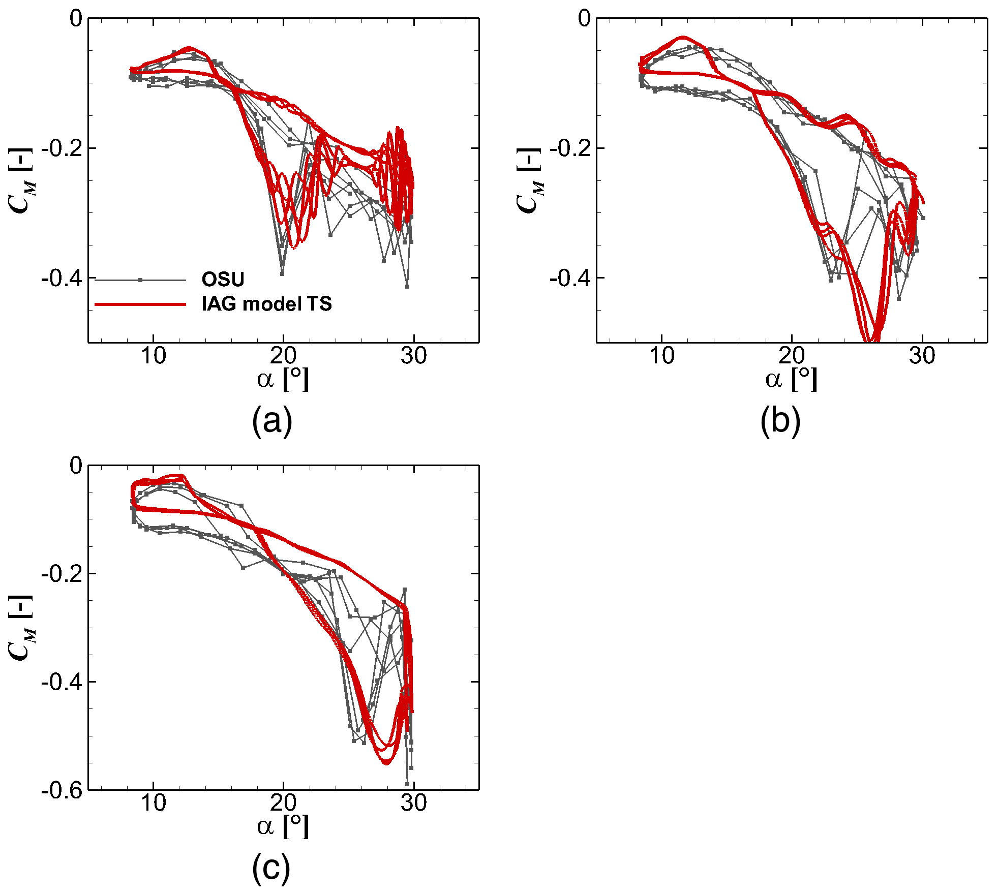
Figure 17 Pitching moment reconstruction by the IAG model in comparison with the measurement data (Ramsay et al., 1996) for $\mathrm{\Delta }t=T/\mathrm{1440}$ using the actual angle of attack in the experimental campaign at various k values. From (a) to (c): k=0.036, k=0.073 and k=0.111. S801 airfoil, $\stackrel{\mathrm{‾}}{\mathit{\alpha }}=\mathrm{20}$ and $\mathrm{\Delta }\mathit{\alpha }=\mathrm{10}{}^{\circ }$.

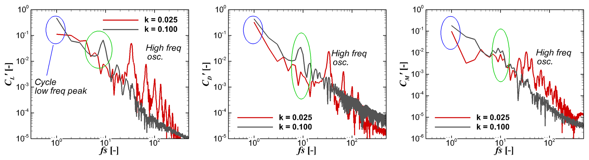
To better investigate the effects of k, the IAG model is used to reconstruct the dynamic polar data at various k values by applying an idealized sinusoidal motion as presented in Fig. 18. Only the last DS cycle is shown for clarity of the observation. While the maximum amplitude of all three force components at low-frequency domains increases with increasing k (blue and green markers), the amplitudes for all three forces at high-frequency domains show different characteristics as shown in the Fourier transformation in Fig. 19, albeit with much smaller values. The higher harmonic amplitudes are attributed to flow separation effects, while for low-frequency domains are driven by the pitching motion (i.e., external unsteadiness or inflow).

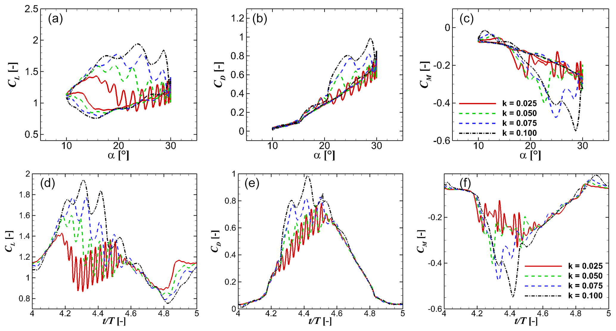
Figure 18 Effects of k on the aerodynamic response by the IAG model for $\mathrm{\Delta }t=T/\mathrm{1440}$. S801 airfoil, $\stackrel{\mathrm{‾}}{\mathit{\alpha }}=\mathrm{20}$ and $\mathrm{\Delta }\mathit{\alpha }=\mathrm{10}{}^{\circ }$. (a–c) Polar; (d–f) time series.

Figure 19 Fourier transformation of the predicted forces presented in Fig. 18. $f_{\mathrm{s}}=f/f_{\mathrm{0}}$ with f₀ being the pitching frequency.

3.5 Performance of the model for different pitching amplitudes

In this section, the effects of pitching amplitude on the aerodynamic response of a pitching airfoil are investigated. The mean angle of attack is fixed at $\stackrel{\mathrm{‾}}{\mathit{\alpha }}=\mathrm{20}{}^{\circ }$. Note again that $\stackrel{\mathrm{‾}}{\mathit{\alpha }}$ is only an approximation because the actual time signal data from the measurement campaign are applied. This large mean angle of attack is purposely selected because the post-stall characteristic is of interest and is well known for its violent vibration, even for the static condition. The small amplitude in this case means that the whole pitch oscillation occurs within the stall regime.

Figures 20 to 22 display the dynamic force responses due to pitching motion of the airfoil predicted by the IAG model in comparison with the experimental data. The model accurately reconstructs the dynamic forces despite the predicted case being challenging within the post-stall regime. Interesting to note is that the small-pitching-amplitude case induces stronger shedding effects for lift than the larger-amplitude case. This can be explained as follows. As described by Leishman in his papers (Beddoes, 1982; Leishman, 1988; Leishman and Beddoes, 1989), the airfoil sees a lagged force response compared to the imposed disturbance. Therefore, in his model, a time-lagged angle of attack is introduced as the “effective” angle actually seen by the airfoil section. When the pitching motion takes place partly within the fully separated region (in the static case) and partly in the attached/partly separated flow region, the airfoil still sees the lower angle (where the flow is still attached) even though the pitching motion already reaches the post-stall regime. This effect stops/decreases when the effective angle is larger than the critical angle defined in Table 4. As the critical angle for the S801 airfoil is defined at 15.1^∘, the lower-amplitude case is fully operating within the stall regime, where the attached flow effect is not present.

Figure 20 Lift reconstruction by the IAG model in comparison with the measurement data (Ramsay et al., 1996) for $\mathrm{\Delta }t=T/\mathrm{1440}$ using the actual angle of attack in the experimental campaign at various Δα values. (a) $\mathrm{\Delta }\mathit{\alpha }=\mathrm{5.5}{}^{\circ }$; (b) $\mathrm{\Delta }\mathit{\alpha }=\mathrm{10}{}^{\circ }$. S801 airfoil, k=0.073 and $\stackrel{\mathrm{‾}}{\mathit{\alpha }}=\mathrm{20}{}^{\circ }$.

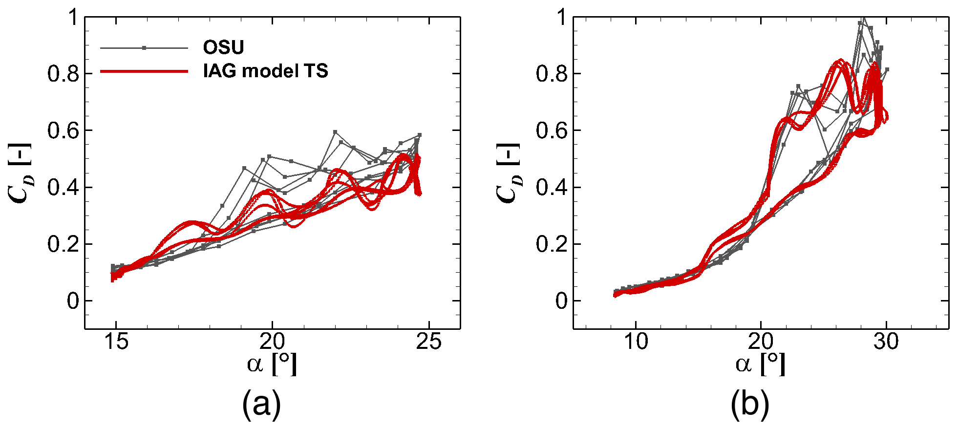
Figure 21 Drag reconstruction by the IAG model in comparison with the measurement data (Ramsay et al., 1996) for $\mathrm{\Delta }t=T/\mathrm{1440}$ using the actual angle of attack in the experimental campaign at various Δα values. (a) $\mathrm{\Delta }\mathit{\alpha }=\mathrm{5.5}{}^{\circ }$; (b) $\mathrm{\Delta }\mathit{\alpha }=\mathrm{10}{}^{\circ }$. S801 airfoil, k=0.073 and $\stackrel{\mathrm{‾}}{\mathit{\alpha }}=\mathrm{20}{}^{\circ }$.

Figure 22 Pitching moment reconstruction by the IAG model in comparison with the measurement data (Ramsay et al., 1996) for $\mathrm{\Delta }t=T/\mathrm{1440}$ using the actual angle of attack in the experimental campaign at various Δα values. (a) $\mathrm{\Delta }\mathit{\alpha }=\mathrm{5.5}{}^{\circ }$; (b) $\mathrm{\Delta }\mathit{\alpha }=\mathrm{10}{}^{\circ }$. S801 airfoil, k=0.073 and $\stackrel{\mathrm{‾}}{\mathit{\alpha }}=\mathrm{20}{}^{\circ }$.

3.6 Performance of the model for different airfoils

In this section, the performance and robustness of the proposed IAG model are assessed for airfoils with different relative thickness. All model constants in Table 3 remain the same for all calculations. The difference from one airfoil calculation to the other lies only in the critical angle of attack value as shown in Table 4. The value was obtained simply by looking at the static polar data where the viscous pitching moment breaks or when the drag increases significantly.

Despite the increased airfoil thickness from 13.5 % to 24 %, Figs. 23 to 25 demonstrate that the reconstructed dynamic forces are in a good agreement with the experimental data, not only for the general trend but also the higher harmonic effects. As is also the case for the Leishman–Beddoes model, it is important to select the appropriate value for the critical angle of attack. The simple approach used in the present paper has shown its usefulness and potentially reduces the complexity of parameter tuning for industrial applications. Elgammi and Sant (2016) for example defined two different critical angles of attack, one for C_N and the other for C_T that were shown to improve the prediction accuracy. Although their attempt might be beneficial, this is not followed in this work because one main aim of the studies is to reduce parameter tuning required for one case to the other cases.

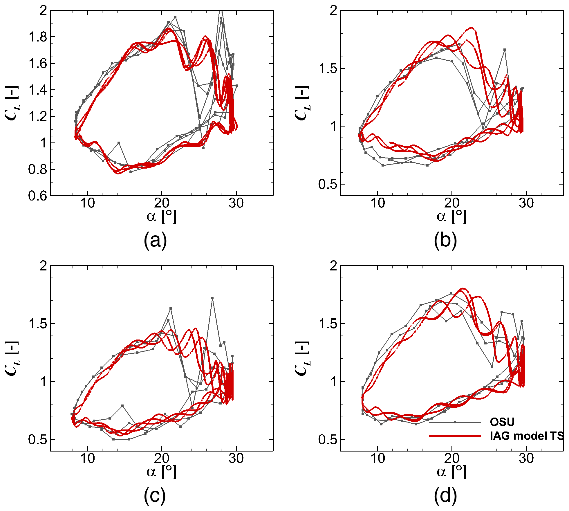
Figure 23 Lift reconstruction by the IAG model in comparison with the measurement data (Ramsay et al., 1996; Hoffman et al., 1996; Ramsay et al., 1995; Janiszewska et al., 1996) for $\mathrm{\Delta }t=T/\mathrm{1440}$ using the actual angle of attack in the experimental campaign for different airfoils. From (a) to (d): S801 (13.5 %), NACA4415 (15 %), S809 (21 %) and S814 (24 %). k=0.073, $\stackrel{\mathrm{‾}}{\mathit{\alpha }}=\mathrm{20}{}^{\circ }$ and $\mathrm{\Delta }\mathit{\alpha }=\mathrm{10}{}^{\circ }$.

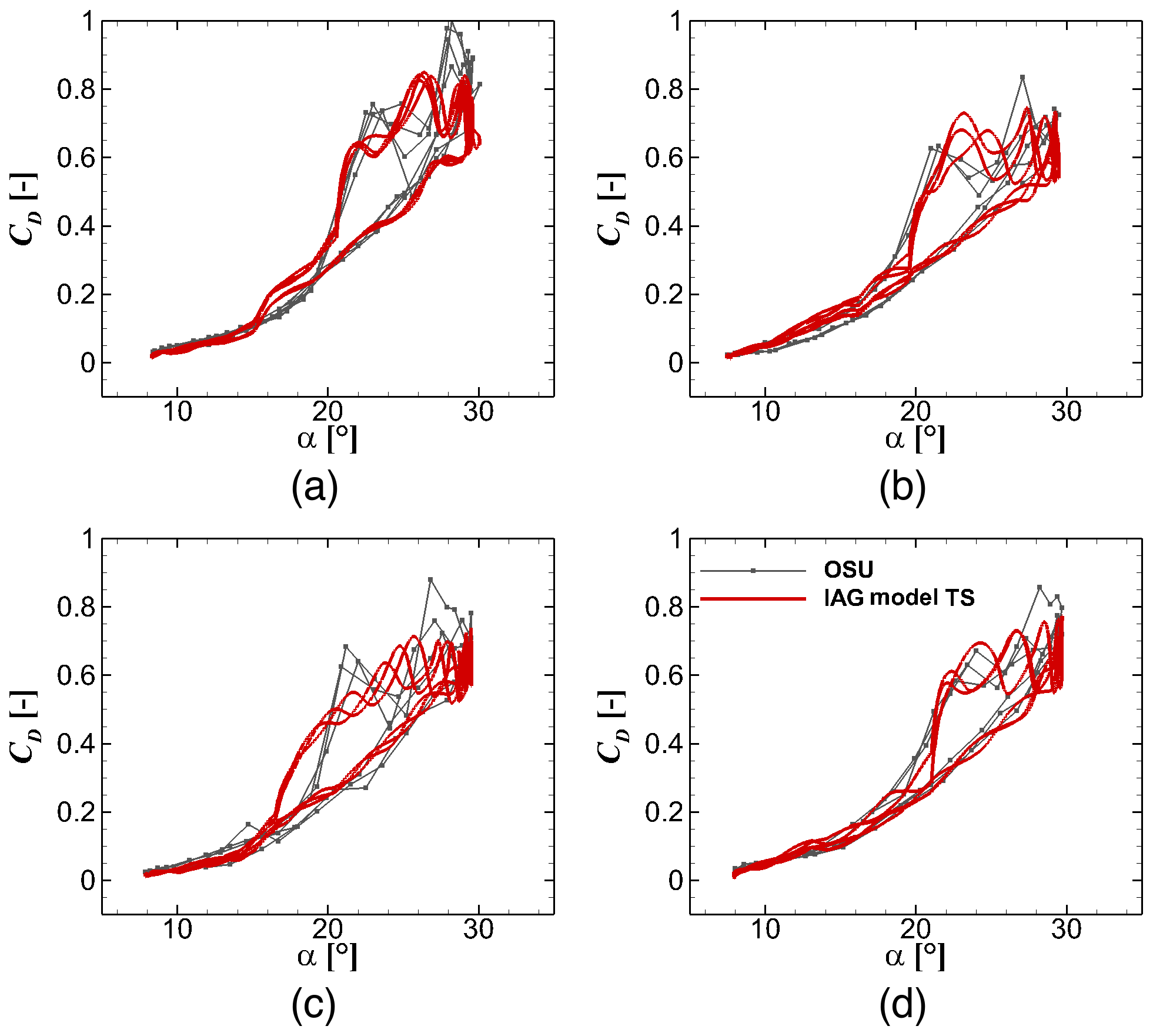
Figure 24 Drag reconstruction by the IAG model in comparison with the measurement data (Ramsay et al., 1996; Hoffman et al., 1996; Ramsay et al., 1995; Janiszewska et al., 1996) for $\mathrm{\Delta }t=T/\mathrm{1440}$ using the actual angle of attack in the experimental campaign for different airfoils. From (a) to (d): S801 (13.5 %), NACA4415 (15 %), S809 (21 %) and S814 (24 %). k=0.073, $\stackrel{\mathrm{‾}}{\mathit{\alpha }}=\mathrm{20}{}^{\circ }$ and $\mathrm{\Delta }\mathit{\alpha }=\mathrm{10}{}^{\circ }$.

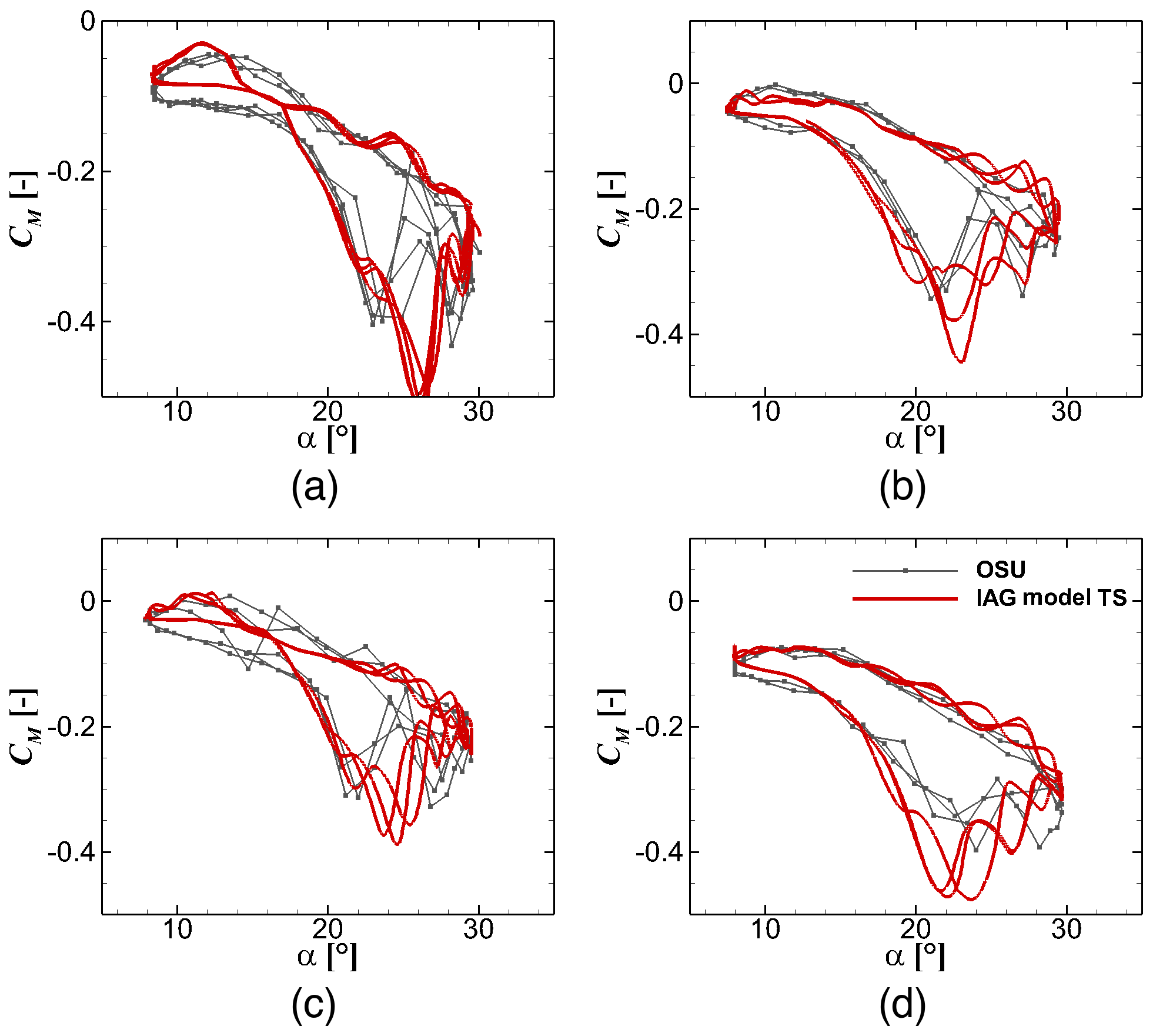
Figure 25 Pitching moment reconstruction by the IAG model in comparison with the measurement data (Ramsay et al., 1996; Hoffman et al., 1996; Ramsay et al., 1995; Janiszewska et al., 1996) for $\mathrm{\Delta }t=T/\mathrm{1440}$ using the actual angle of attack in the experimental campaign for different airfoils. From (a) to (d): S801 (13.5 %), NACA4415 (15 %), S809 (21 %) and S814 (24 %). k=0.073, $\stackrel{\mathrm{‾}}{\mathit{\alpha }}=\mathrm{20}{}^{\circ }$ and $\mathrm{\Delta }\mathit{\alpha }=\mathrm{10}{}^{\circ }$.

3.7 Predictions of the center of pressure

To further complement the analyses conducted in Sect. 3.6, the location of the actual pressure center is calculated in this section as

$$\begin{array}{}\text{(78)}& X_{\mathrm{p}}=-{\displaystyle \frac{C_{\mathrm{M}}}{C_{\mathrm{L}}}},\end{array}$$

which indicates the distance of the pressure point to the quarter chord position where C_M is defined.

A correct location of the pressure point is important for determining the stability on aeroelastic simulations of wind turbine blades. The results of the calculations both for the experimental data and for the proposed IAG model are presented in Fig. 26 for all four investigated airfoils both as time series and as the polar plot. It can be seen clearly that the agreement between the experimental data and the present predictions is excellent for all investigated airfoils.

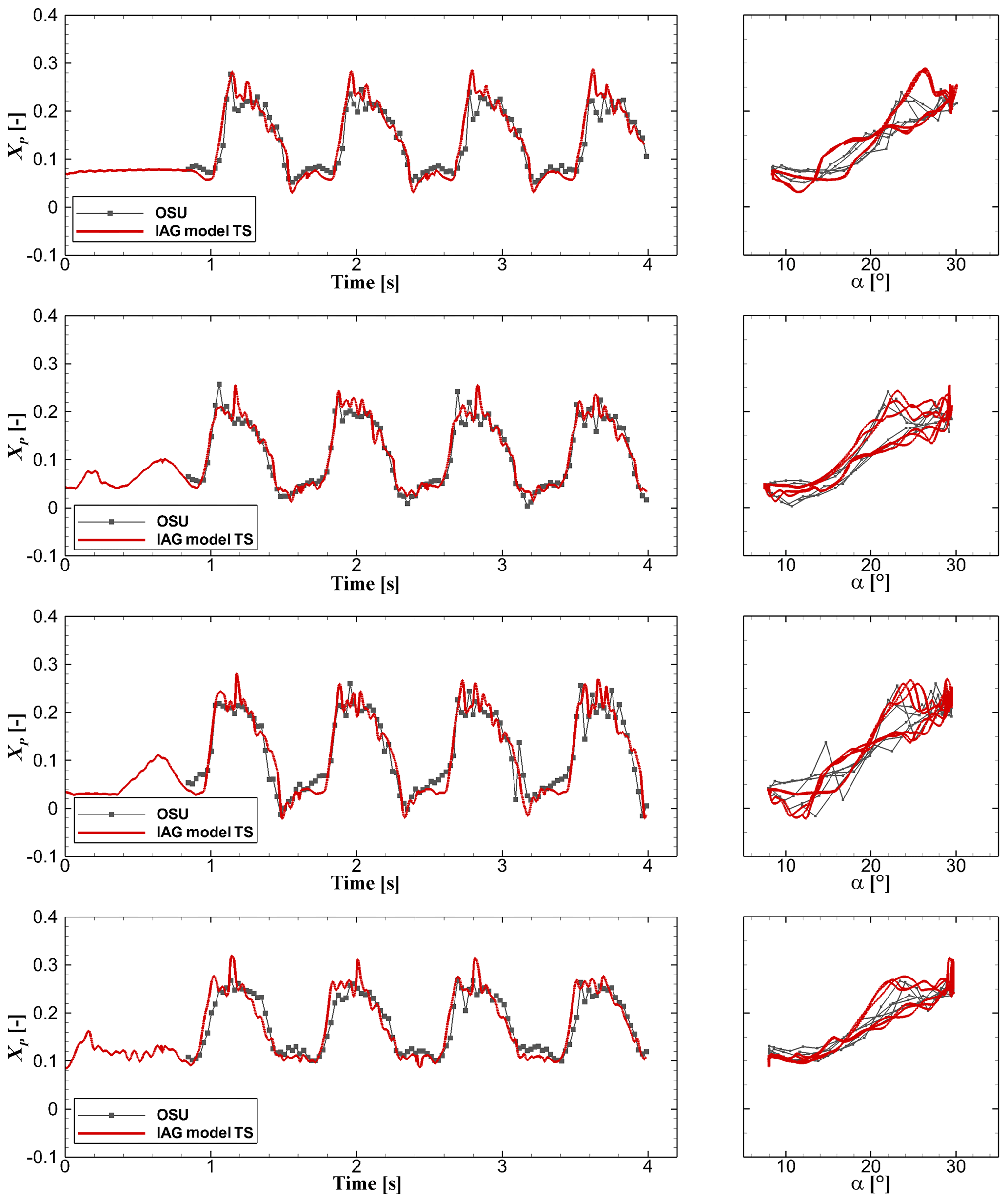
Figure 26 Center of pressure reconstruction in comparison with the measurement data by the IAG model for $\mathrm{\Delta }t=T/\mathrm{1440}$ using the actual angle of attack in the experimental campaign for different airfoils. From top to bottom: S801 (13.5 %), NACA4415 (15 %), S809 (21 %) and S814 (24 %). k=0.073, $\stackrel{\mathrm{‾}}{\mathit{\alpha }}=\mathrm{2}{}^{\circ }\mathrm{0}$ and $\mathrm{\Delta }\mathit{\alpha }=\mathrm{10}{}^{\circ }$.

3.8 L₂ norm of error analyses

Holierhoek et al. (2013) introduced a way of quantifying the absolute error between the experimental data and modeled lift coefficient. The general formulation reads

$$\begin{array}{}\text{(79)}& L_{\mathrm{2}}^{\mathit{\varphi }}=\sqrt{{\displaystyle \frac{\mathrm{1}}{N}}\sum _i^N{\left({\mathit{\varphi }}_i^{\mathrm{mod}}-{\mathit{\varphi }}_i^{\exp }\right)}^{\mathrm{2}}},\end{array}$$

with ϕ being the variable of interest, i the current sample and N the total number of samples. In their paper, however, only lift was considered. Here all three force components will be shown for four different airfoils. Figure 27 displays the quantified error for two different flow categories, attached and deep stall. The time series of the angle of attack was obtained from the measured data by applying a third-order cubic-spline interpolation in between each available point. One can see that generally the attached flow case is predicted very well, while the error increases as the flow condition becomes more complicated. Interestingly, especially for lift, it seems that the error decreases with increasing airfoil thickness. The reason for the larger error obtained for the thinner airfoil is attributed to the complex characteristics of the leading edge stall, causing severe load variations, especially with increasing angle of attack. Thus, it makes the prediction more challenging. Furthermore, the quantification of the error was also performed on two other dynamic stall models, Snel and Adema–Snel. The same approach for the angle of attack signal was applied. One can see that the IAG model shows its improved prediction in particular for the deep-stall case for all three force components.

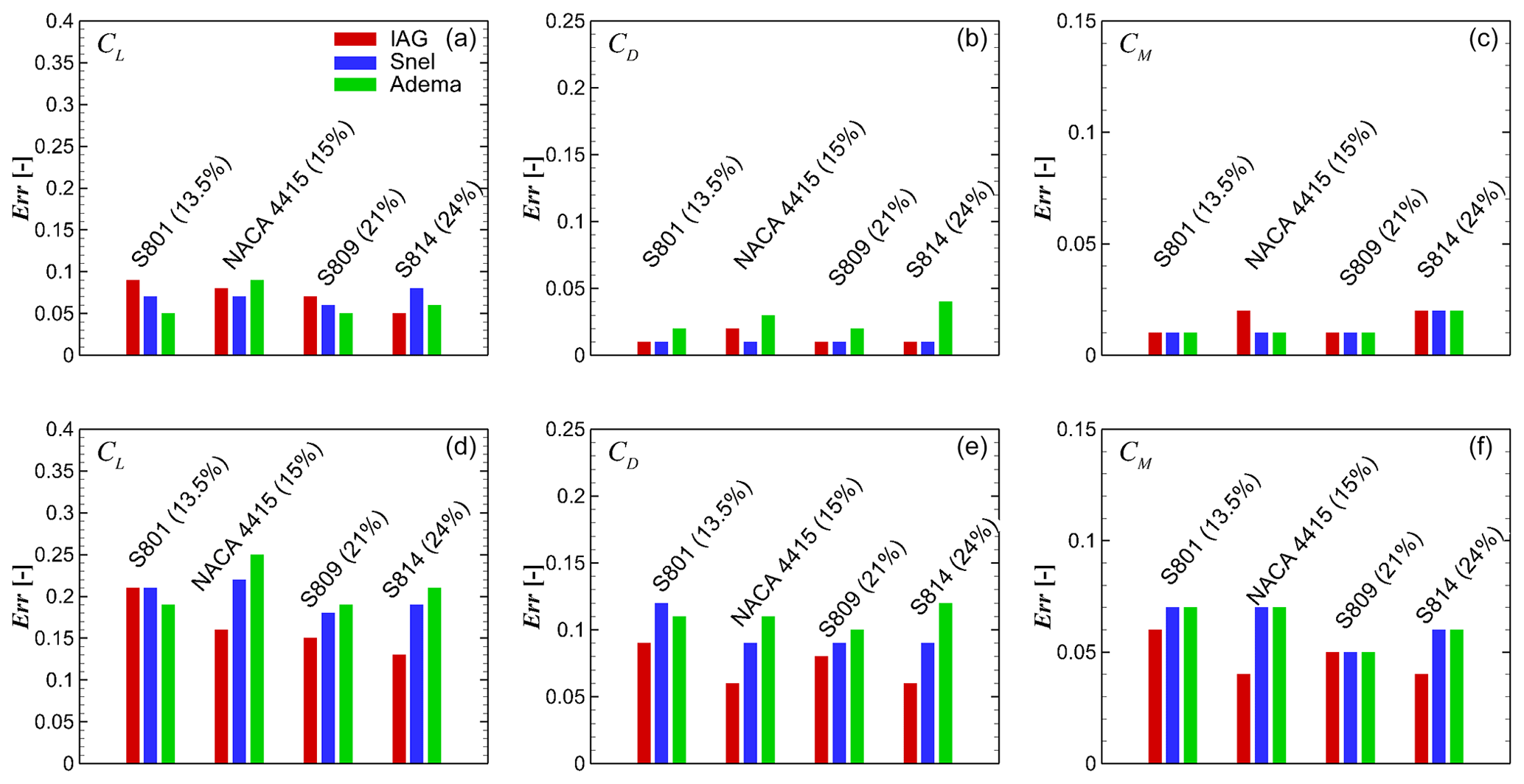
Figure 27 Quantified L₂ norm of error with respect to the measurement data for four airfoils. (a–c) Attached flow case (k=0.073, $\stackrel{\mathrm{‾}}{\mathit{\alpha }}=\mathrm{8}{}^{\circ }$, $\mathrm{\Delta }\mathit{\alpha }=\mathrm{5.5}{}^{\circ }$); (d–f) deep-stall case (k=0.073, $\stackrel{\mathrm{‾}}{\mathit{\alpha }}=\mathrm{20}{}^{\circ }$, $\mathrm{\Delta }\mathit{\alpha }=\mathrm{10}{}^{\circ }$).

4 Conclusions

Comprehensive studies on the accuracy of several state-of-the-art dynamic models to predict the aerodynamic loads of a pitching airfoil have been conducted. From the studies, the strength and weaknesses of each model were highlighted. This information was then transferred to develop a new second-order dynamic stall model proposed in this paper. The new model improves the prediction for the aerodynamic forces and their higher-harmonic effects due to vortex shedding, developed for robustness to improve its usability in practical wind turbine calculations. Details on the model characteristics, modifications and treatment for numerical implementation were summarized in the present paper. The studies were conducted by examining the influence of the time step size, time signal deviation, mean angle of attack, reduced frequency, pitching amplitude and variation in the airfoil thickness. Several main conclusions can be drawn from the work.

• The general characteristics of the polar data can be predicted by all investigated dynamic stall models. Despite that, only the Adema model and the present IAG model are able to demonstrate the higher harmonic effects among the three investigated models.

• The exact time signal imposed based on the measurement campaign improves the prediction accuracy of the IAG model in comparison with the idealized sinusoidal motion.

• The dynamic forces reconstructed by the IAG model are in a sound agreement with the experimental data under various flow conditions by variation in $\stackrel{\mathrm{‾}}{\mathit{\alpha }}$, k and Δα and for four different airfoils by changing only the values of the critical angle of attack.

• The amplitudes at low-frequency domains increase with increasing k and can be attributed to the effects of inflow/external unsteadiness. The amplitudes at high-frequency domains decrease with increasing k values, which are driven by flow separation effects.

• When the airfoil operates at a high $\stackrel{\mathrm{‾}}{\mathit{\alpha }}$ within the stall regime, a small Δα leads to increased vibrations for lift. The opposite is true for the pitching moment.

5 Recommendations for future work

The present paper evaluates the newly developed IAG model under various flow conditions for four different airfoils. The following aspects are encouraged for future work.

• In the present studies, the assessment was mainly carried out for the S801 airfoil having a relative thickness of 13.5 %. This airfoil is mainly characterized by leading edge separation, which is very challenging for validating the accuracy of a dynamic stall model. However, typical modern wind turbine blades usually employ airfoils with no less than 18 % relative thickness and a much higher Reynolds number. Therefore, future investigations shall be done for thicker airfoils at various flow conditions as well.

• The above statement is also true for the current available experimental data. Therefore, experiments on dynamic stall for thick airfoils at a much higher Reynolds number are encouraged.

• Three-dimensional effects (Himmelskamp or tip loss effects) for a rotating blade can alter the loads significantly even under a steady inflow condition. Further consideration and examination of the model under this condition shall be carried out.

• Further tests and recalibration of the model for deep-stall conditions at extremely large angles of attack are encouraged, which can be relevant for a turbine in standstill.

Appendix A: List of symbols

Variables
s	Nondimensional time (s)
V	Incoming wind speed (m s−1)
t	Time (s)
c	Chord (m)
CN	Normal force coefficient (–)
CT	Tangential force coefficient (–)
CL	Lift force coefficient (–)
CD	Drag force coefficient (–)
CM	Pitching moment coefficient (–)
$C_{\mathrm{N}}^{\mathrm{P}}$	Total inviscid CN (–)
$C_{\mathrm{N}}^{\mathrm{P}\mathrm{1}}$	Time-lagged total inviscid CN (–)
$C_{\mathrm{N}}^{\mathrm{I}}$	Impulsive inviscid CN (–)
$C_{\mathrm{N}}^{\mathrm{C}}$	Circulatory inviscid CN (–)
$C_{\mathrm{N}}^{\mathrm{f}}$	Viscous CN (–)
$C_{\mathrm{T}}^{\mathrm{f}}$	Viscous tangential force coefficient (–)
$C_{\mathrm{M}}^{\mathrm{f}}$	Viscous pitching moment coefficient (–)
$C_{\mathrm{M}}^{\mathrm{C}}$	Circulatory pitching moment coefficient (–)
$C_{\mathrm{N}}^{\mathrm{V}}$	Vortex lift CN (–)
$C_{\mathrm{N}}^{\mathrm{CRIT}}$	Critical CN (–)
CPf	Stepping parameter moment (–)
f	Frequency (Hz)
f0	Pitching frequency (Hz)
fn, f1, f2	Separation factor (–)
F1, F2	First- and second-order forcing term (–)
k	Reduced frequency ($k=\mathit{\pi }{f}_{\mathrm{0}}c/V$) (–)
Kf	Stiffness coefficient (–)
ks	Constant close to Strouhal number (–)
M	Mach number (–)
X, Y, D	Deficiency functions (–)
c1, c2, c3	Curve-fitting constants (–)
a1, a2, a3	Curve-fitting constants (–)
S1, S2, S3, α1	Curve-fitting constants (–)
A1, A2, b1, b2	Model constants (–)
Kα, Tp, Tf, Tv, Tvl	Model constants (–)
Kv, η, $K_{\mathrm{f}}^{\mathrm{C}}$, $T_{\mathrm{m}}^{\mathrm{U}}$, $T_{\mathrm{m}}^{\mathrm{D}}$	Model constants (–)
Greek letters
α	Angle of attack (rad (unless stated otherwise))
α0	Zero lift α (rad (unless stated otherwise))
αe	Effective α (rad (unless stated otherwise))
αf	Time-lagged αe (rad (unless stated otherwise))
αCRIT	Critical α (rad (unless stated otherwise))
β	Mach-number-dependent parameter (–)
τv	Nondimensional vortex time (–)
τ	Time constant (–)
ζv	Vortex lift drag limiting factor (–)
Subscripts
n	Present sampling time (–)
f	Viscous lagged value (–)
v	Vortex lift affected value (–)

Superscripts
INV	Static inviscid (–)
VISC	Static viscous (–)
I	Impulsive (–)
CRIT	Critical (–)
D	Dynamic loading (–)
D1	First-order correction (–)
D2	Second-order correction (–)