the Creative Commons Attribution 4.0 License.
the Creative Commons Attribution 4.0 License.
 | 23 Sep 2020
Multipoint reconstruction of wind speeds
Christian Behnken
Matthias Wächter
The most intermittent behaviour of atmospheric turbulence is found for very short timescales. Based on a concatenation of conditional probability density functions (cpdf's) of nested wind speed increments, inspired by a Markov process in scale, we derive a short-time predictor for wind speed fluctuations around a non-stationary mean value and with a corresponding non-stationary variance. As a new quality this short-time predictor enables a multipoint reconstruction of wind data. The used cpdf's are (1) directly estimated from historical data from the offshore research platform FINO1 and (2) obtained from numerical solutions of a family of Fokker–Planck equations in the scale domain. The explicit forms of the Fokker–Planck equations are estimated from the given wind data. A good agreement between the statistics of the generated and measured synthetic wind speed fluctuations is found even on timescales below 1 s. This shows that our approach captures the short-time dynamics of real wind speed fluctuations very well. Our method is extended by taking the non-stationarity of the mean wind speed and its non-stationary variance into account.
- Article
(3311 KB) - Full-text XML
- BibTeX
- EndNote


The transition of our energy system, formerly strongly relying on gas and coal, to a decarbonised one, mainly based on wind, solar and hydropower, is still ongoing work, but great progress has been made. From 2005 to 2017 the share in installed capacity of wind (solar) has been increased from 6 % (0.3 %) to 18 % (11.5 %) in the European Union (WindEurope, 2018). The downside of this increasing share of fluctuating renewable energy sources is their integration into the power grid. By analysing measurements of fed-in wind and solar power, it could be shown that their fluctuations strongly deviate from Gaussian behaviour on timescales ranging from hours to seconds (Anvari et al., 2016) and for wind power even for scales below 1 s (Haehne et al., 2018). This survival of the atmospheric intermittency in the power grid poses the grid operators with the great challenge to ensure stable power supply, even under highly volatile conditions. Within this context the term intermittency is used in the spirit of Kolmogorov (1962) to describe the characteristic heavy-tailed shape of pdf's often found at small scales in time series of turbulent systems (Frisch, 2004).
To aid the design of our future energy systems, for example to size the needed energy storage or the power generation capacity of conventional power plants, much work has been done in the field of long-term wind speed and power modelling, utilising Markov chain models. Whereas simple first-order Markov chain models cannot grasp the characteristics of long-term correlations of wind speeds (Brokish and Kirtley, 2009), higher-order Markov chain models perform better, but will require more input data for estimating the transition matrices or some simplifications (Pesch et al., 2015; Brokish and Kirtley, 2009; Papaefthymiou and Klockl, 2008; Weber et al., 2018).
Despite their dramatic effect of long-range correlation and fluctuations of wind speeds on the power generation (and thus the grid stability), wind speed fluctuations are known to be most intermittent on short timescales (Boettcher et al., 2003). With short timescales we refer to timescales in the range of seconds to minutes. As can be seen in Boettcher et al. (2003), the effect of intermittency is most prominent at timescales <1 s, but as the timescales increase, the pdf's broaden. Models considering time steps ranging from minutes to seconds or even below are of course not suited for energy system analysis on national levels, but they are useful tools for wind turbine operators. For a time step of 10 min Carpinone et al. (2010) presented a higher-order Markov chain model for wind power, and Milan et al. (2013) showed a stochastic power model based on a conditional Langevin equation to work even in the range of seconds.
The knowledge of full three-dimensional wind fields for all three velocity components and the pressure in all details would be desirable. The lack of basic understanding, the impracticability of handling such huge data sets and the complexity of the wind energy conversion process often lead to the demand for simplified models for wind speed. Common approaches for the design of wind turbines are the so-called Mann uniform shear and the Kaimal spectral and exponential coherence model (IEC, 2005). Both models take spectral and coherence aspects of turbulent velocity fluctuations into account, thus handling the fluctuations as Gaussian distributed and stationary. Higher-order statistical effects like the prominent intermittency effect of turbulence and non-stationarities are not taken into account; see for example Mücke et al. (2011). Another approach is to use one-dimensional effective wind speed time series, representing for example the wind field together with the rotor aerodynamics as it impacts the drivetrain or can be used to model the above-discussed energy conversion process (Wächter et al., 2011).
Within this work we propose a novel stochastic generator of one-dimensional wind speed fluctuations with a sampling interval of 0.1 s. One main novelty is that we show how to grasp by this model multipoint statistics of wind structures in time. While commonly applied methods, like spectral analysis and two-point correlations, limit themselves to two-point statistics, here we extend the methodology to more than two points in time. We obtain generalised correlations between multiple points in time, in terms of probability density functions (pdf's), for the occurrence of a whole sequence of wind speeds. Those pdf's we denote multipoint pdf's, and they constitute the basic concept of our approach. Such a stochastic multipoint approach should in principle be able to grasp wind structures like gusts as well as clustering of wind fluctuations. The method was initially developed by Nawroth and Peinke (2006) in the context of homogeneous isotropic turbulence and later on applied to the modelling of log-return rates of current exchange rates (Nawroth et al., 2010) and velocity increments of idealised homogeneous isotropic turbulence (Stresing and Peinke, 2010). The successful application to ocean gravity waves (Hadjihosseini et al., 2016) showed that structures of monster waves can be grasped by this approach correctly (Hadjihoseini et al., 2018). For a recent review see (Peinke et al., 2019). Finally we want to point out that we also show how to handle the aspect of non-stationary wind conditions.
We will continue as follows. In the first part we discuss the method for a subset of wind data characterised by its mean wind speed and its standard deviation. For such data it is shown how, arising from a Langevin process in scale, a predictor for the upcoming wind speed fluctuation around a mean value can be derived by a nesting of conditional probability density functions. Afterwards we check for Markovian properties of the wind speed fluctuations in scale and set up a Fokker–Planck equation, corresponding to the Langevin process in scale, and we show how it contributes to the improvement of our stochastic prediction method. Finally, in the second part, the non-stationary mean wind speed and its non-stationary variance are incorporated into our approach to achieve more realistic wind speed time series.
In this section we present the stochastic framework used for our multipoint reconstruction scheme. As a simplification we start this discussion for blocks of wind data U(t), with the time t, which share the same mean wind speed and the same standard deviation σU, as suggested in Morales et al. (2012). Fixing and σU one would generate quasi-stationary subsets of data. We follow this idea, but instead of creating quasi-stationary subsets, we aim at creating quasi-stationary time series. With U(t) we refer to the resulting wind speed from the horizontal components. The quasi-stationary wind speed u(t) is then obtained from U(t) by normalising it with the mean and standard deviation σU within blocks of 1 min length. We use measured data from the offshore research platform FINO1: the data were recorded at a sampling frequency of 1 Hz between calendar weeks 1 and 10 in 2007 with an ultrasonic anemometer, mounted at 80 m height, resulting in approximately 6×10⁶ samples. The use of our method for non-stationary time series is outlined in Sect. 3.
2.1 Multipoint statistics
Since we assume wind speeds to emerge from a turbulent cascade, increments will play a key role in our method. Having a time series of wind speeds u(t), the corresponding increment time series Δu(τ), depending on a certain scale τ, is given by
This is the definition of so-called right-sided increments. Note that the calculation of Δu(τ) after this definition depends on the current wind speed u(t) and a past value u(t−τ), whereas the use of left-sided increments would premise the knowledge of future values u(t+τ), creating a contradiction as we aim at producing synthetic wind speed time series. To ease readability we use the shorthand notations and with () in the following.
As a further remark we note that although we consider in this work time series of wind speed, we often talk of multipoint statistics. Δu(τ) is considered to be a statistical two-point quantity, which more correctly could be denoted as a two-time quantity. Based on the commonly used hypotheses on frozen turbulence by Taylor, for short-time fluctuations time and space statistics are related linearly by the mean wind speed (see also Peinke et al., 2019).
Our idea is to predict a wind speed only by knowledge of its N past values . The probability of an event u* to happen at time t* can then be expressed by the conditional probability density function (cpdf)
using the definition of conditional probabilities. Note this cpdf is the key quantity to estimate a new wind speed value u*, and it can be used iteratively to generate new time series, as we show below.
Now we link Eq. (2) to the idea of an underlying turbulent cascade, which can be described by means of a Markov process. Thus we assume that there exists a scale separation (j>i), after which the Markov condition is fulfilled for all greater scales. This scale separation ΔτME is often called the Markov–Einstein length (Einstein, 1905). It enables us to express the multiple cpdf by a multiplication of a simpler double cpdf and marginal pdf's:
with with the timescale τi−τ1. For details we refer the reader to Appendix A.
It is known that the evolution of cpdf's of a Markov process can be described by the famous Kramers–Moyal expansion (Risken, 1996), which notes for our stochastic process in scale Δui
requiring and with the Kramers–Moyal coefficients D(n) being defined as
In contrast to the Kramers–Moyal expansion in time domain, a minus sign on the left-hand side (lhs) of Eq. (4) has to be added for scale processes, since during evolution of the process the scale τ is decreasing. According to the Pawula theorem, the Kramers–Moyal coefficients vanish for n≥3, if D(4)=0 (Risken, 1996); thus the Kramers–Moyal expansion reduces to the Fokker–Planck equation (FPE):
with the drift function D(1) accounting for the deterministic evolution of the stochastic process, whereas the so-called diffusion function D(2) scales the amplitude of the noise term of the corresponding Langevin equation
with the Gaussian noise Γ(τ), fulfilling 〈Γ(τ)〉=0 and also . This equation directly describes the evolution of a single trajectory along the scale τ.
As can be seen, the FPE can be used to determine the factorised pdf's from Eq. (3) if the process is Markovian and higher-order Kramers–Moyal coefficients are zero. This equivalence between a cpdf with N conditions and a nested chain of several cpdf's with only two conditions, stemming from the three-point closure of a cascade process, is extremely helpful if one aims at estimating the pdf's from measurements, since the high-dimensional pdf's in Eq. (2) would require a tremendous number of realisations in order to be estimated well. For a more detailed discussion of this multipoint approach we refer to Peinke et al. (2019).
2.2 Preliminary analysis of wind speed data
Next we check if wind speed data are suitable for the reconstruction method just described. According to the right-hand side (rhs) of Eq. (3) the estimation of the double cpdf's is necessary. However, to reduce computational costs or the number of data points, it would be much more convenient to use the single cpdf's by excluding the condition on the wind speed u* to be predicted (Nawroth et al., 2010; Peinke et al., 2019). Thus the equality
must hold. As can be seen from Fig. 1, Eq. (8) holds for but shows a significant shift for . From this we reason that the equality in Eq. (8) cannot generally be assumed, so we have to stick to the double cpdf's . Similar results have been reported for idealised turbulence (Stresing and Peinke, 2010) and sea waves (Hadjihosseini et al., 2016). On derivation of our final formula for the reconstruction of time series (see Eq. 3) an essential step was to premise the underlying scale process to be Markovian. Thus it has to be shown that for
is a valid assumption. As the verification of this expression is not feasible in its generality, we limit ourselves by reducing the number of dimensions involved and just check the equality of
To check this we utilise the Chapman–Kolmogorov equation (CKE) (Friedrich et al., 2011). The cpdf is estimated directly from observational data and afterwards compared with the cpdf obtained numerically by use of the CKE
whereas the two cpdf's within the integral on the rhs are also directly estimated from data. Figure 2 shows that Eq. (11) only holds for Δτ≥ΔτME. We find a Markov–Einstein length of ΔτME≤0.1 s, which we are going to use henceforth.
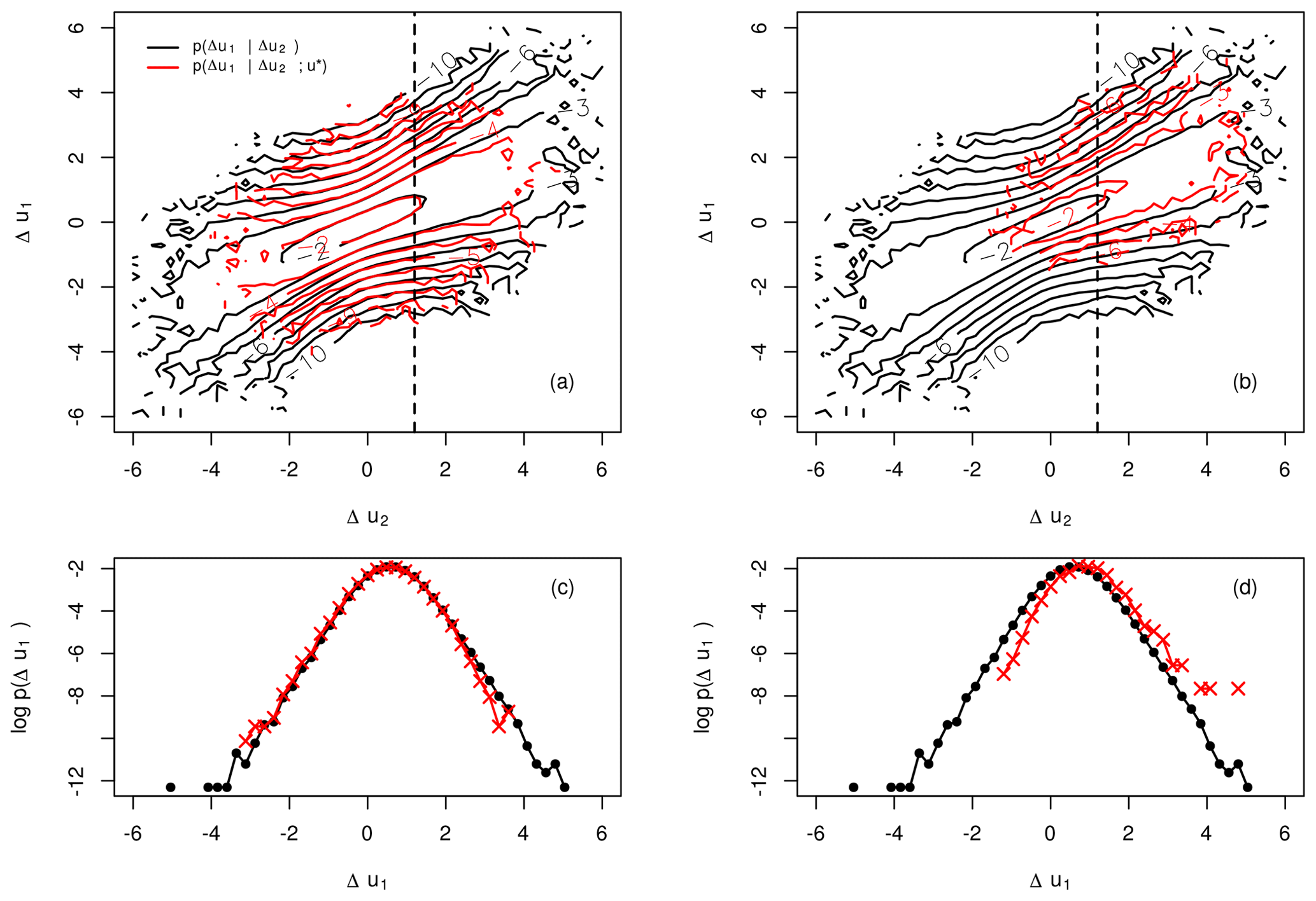
Figure 1Comparison of single cpdf's p(Δu1|Δu2) (black) and double cpdf's (red) for (a, c), (b, d), τ1=1 s and τ2=2τ1. Dashed lines indicate cuts through the cpdf's at Δu2≈1.2. The levels of the contour plots are given in natural logarithmic scale.
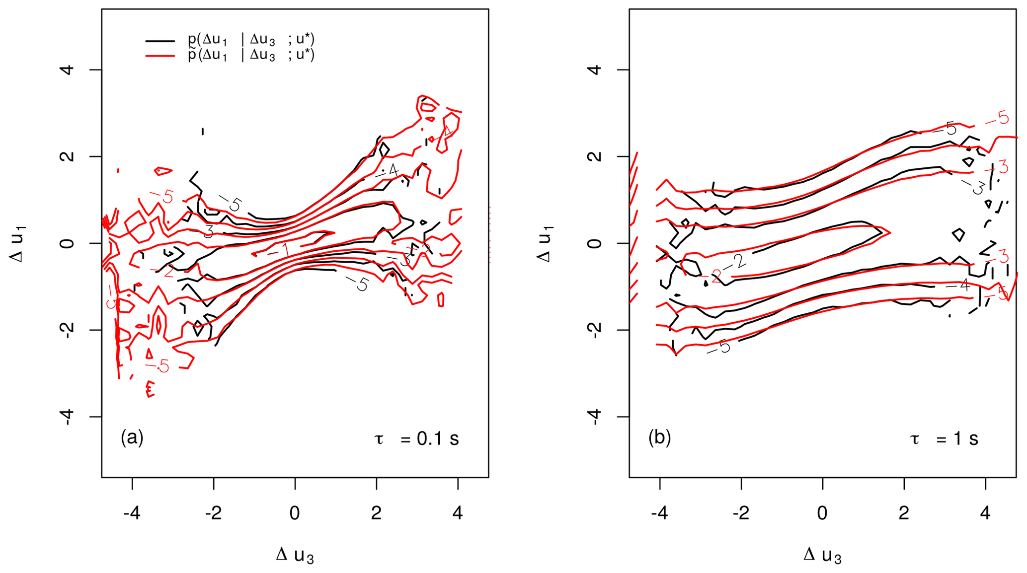
Figure 2Comparison of the double cpdf's (estimated from data) and (obtained from CKE) for τ1=0.1 s (a) or 1 s (b) and τ2=2τ1, τ3=3τ1, and .
2.3 Parameterisation of the Fokker–Planck equation
As was mentioned in Sect. 2.1 the FPE may be used to generate solutions for the needed cpdf's in Eq. (1). Aiming for this, one needs a parameterisation of the FPE reflecting the scale process of the real-world wind speed data. No general, physical formulation for a FPE describing the scale process of wind speeds is known; thus we use the possibility to estimate a parameterisation directly from the given data (compare Eq. 5 and Reinke et al., 2018; Peinke et al., 2019).
This way we obtain estimations of the drift and diffusion functions , along the scale τi and for every wind speed value u*. From these estimations one then usually finds parameterisations of the FPE by fitting appropriate polynomial surfaces to the estimated functions, which then may be used to obtain numerical solutions of the FPE.
To match the functional shape of the estimated and (see Fig. 3), we require the polynomials to be of the order of 3 and 2 respectively. We find a significant shift, denoted with , depending on u* and τi for the drift along all scales τi which has to be taken into account for a parameterisation suitable to the given data.
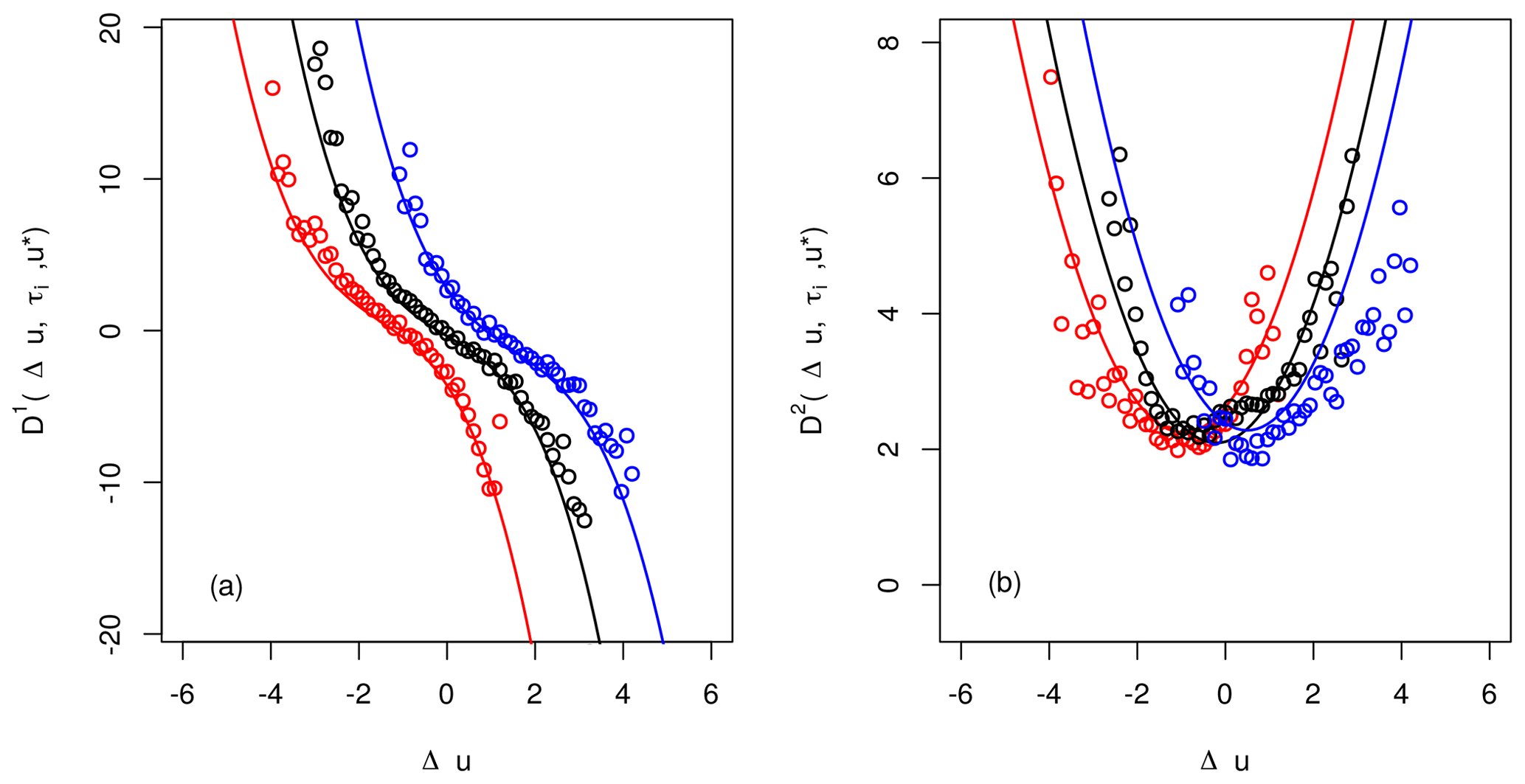
We set for
and for
Similar findings were obtained for other systems (Hadjihosseini et al., 2016; Stresing and Peinke, 2010), where the dependence on u* was limited only to the drift function . For wind speed data the contribution of u* is clearly more complex.
Furthermore we check the validity of the Pawula theorem, requiring D(4)=0. As one can see in Fig. 4, the fourth Kramers–Moyal coefficient is slightly larger than zero, but negligible compared to the magnitude of the diffusion function D(2).
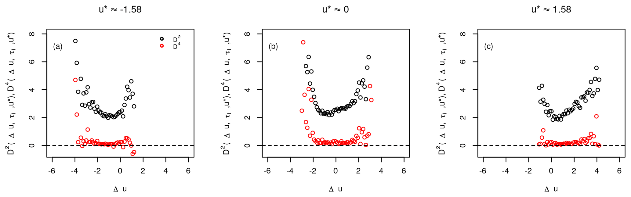
Figure 4Exemplary estimations of the second and fourth Kramers–Moyal coefficients and for τ=65 s.
Next, we check if the parameterisation of the FPE, given by Eqs. (12) and (13), performs well in describing the underlying scale process, before one uses it for the reconstruction scheme presented in Sect. 2.1. This can easily be done by comparing cpdf's estimated directly from the data and the ones obtained from numerical solutions of the FPE. The latter one is not carried out by common finite-difference schemes but by an iterative approach (for first works see Renner et al., 2001; Wächter et al., 2003). For a (very) small step size in scale Δτ the functions and can be assumed to be constant in τ, leading to an exact solution (see Risken, 1996) for the cpdf
describing the transition between wind speed increments of a larger scale τi and a smaller scale τi−Δτ. By iteratively combining this so-called short-time propagator (STP) with the CKE (see Eq. 11), one is able to obtain cpdf's for arbitrary large-scale differences . In theory this procedure would lead to exact solutions of the FPE, but since one is limited to finite step sizes Δτ, this method of course only provides numerical approximations of the true cpdf's.
Comparing cpdf's estimated directly from the data and from the numerical solution, we see (Fig. 5) that our proposed estimation in terms of and is well suited to describe the underlying scale process. Thus we use this parameterisation for the reconstruction scheme.
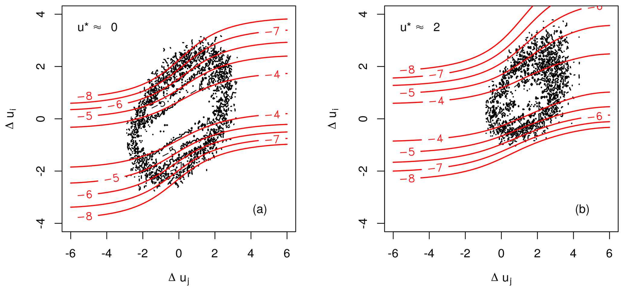
Figure 5Isoline plots of a cpdf estimated from the data (black) and from the numerical solution of the FPE (red) for τi=1.6 s and τj=3.2 s and for and .
2.4 Results of the multiscale reconstruction
Alternatively to the presented approach to obtain the cpdf's from numerical solutions of the FPE, it is of course possible and much less cumbersome to estimate them directly from observational data. (Note that due to the use of the FPE, the obtained pdf's are less noisy and extend to large values as seen in Fig. 5.) In this section we will present the results for the multipoint reconstruction achieved for u*, yielded from both approaches.
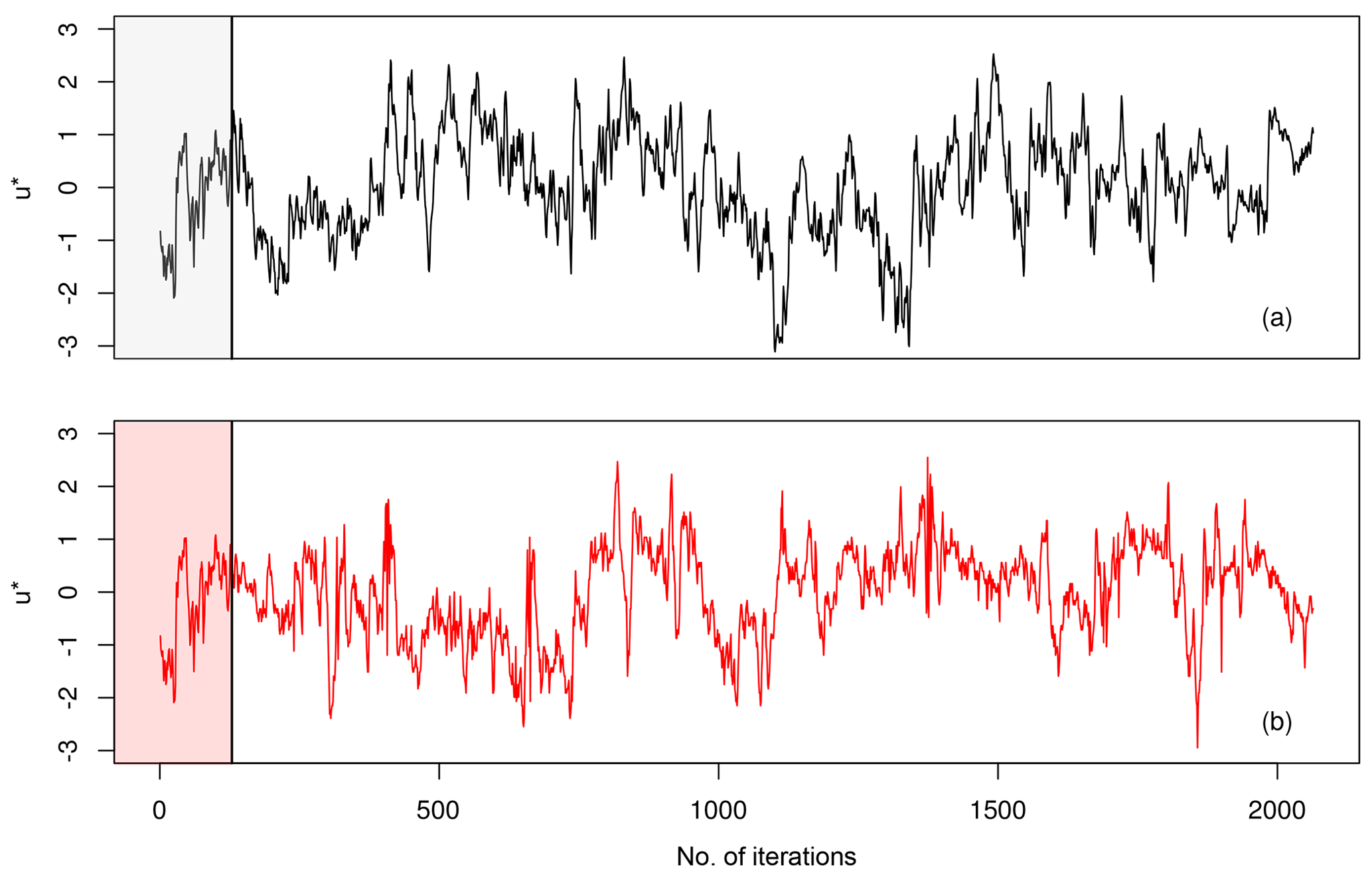
Figure 6Comparison of original wind speed time series u* (black, a) with the reconstructed one using Eq. (8) (red, b). The vertical line marks the transition from the N=128 starting values to the simulated wind speeds.
To start the reconstruction scheme, we provided a short piece of the original time series of N wind speeds to the algorithm to compute the pdf , from which the first point of our simulation can be drawn. The reconstruction scheme is then shifted by one time step τ and applied again. By iteratively applying our method a new artificial time series of arbitrary length can be generated. After N iterations of the reconstruction scheme no data from measurements are required any more to generate new values of u*. From visual comparison in Fig. 6 one finds a realistic looking simulated time series of u*, retaining the characteristics of dynamics on the smaller scales as well as the ones of the larger scales.
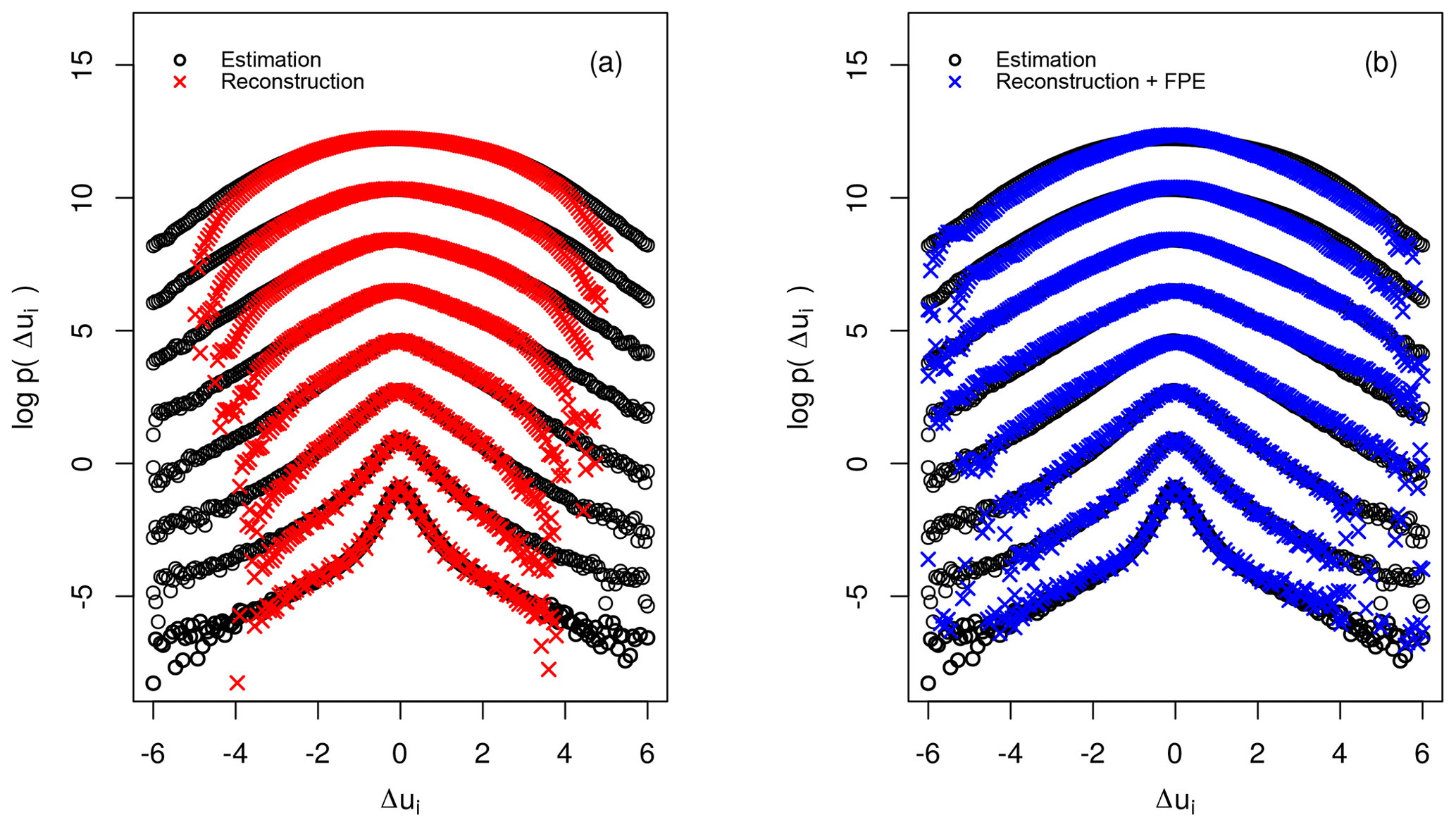
Figure 7Comparison of the marginal increment pdf's computed from the empirical data (black), the simulated data using the directly estimated pdf's (red) and the simulated data using the cpdf's obtained from numerical solution of the FPE (blue). The scales range from ΔτME to N⋅τME; they are explicitly: 2i⋅ΔτME with and ΔτME=0.1 s. For better visualisation the pdf's were shifted along the vertical axis.
To confirm this visual impression in a quantitative way, we compare the increment pdf's p(Δui,τi) obtained from the reconstructed and the measured time series. The synthetic time series were generated by using the cpdf's estimated directly both from data and from numerical solutions of the FPE.
As shown in Fig. 7 the increment pdf's yielded from both stochastic simulations nicely coincide with the pdf's from observations. This attests that the presented reconstruction scheme is able to capture the complex dynamics of wind speeds, characterised by a gradual shift of increment pdf's of a Gaussian-like shape (larger scales) to increment pdf's of a heavy-tailed shape (smaller scales).
A striking difference between the increment pdf's from the stochastic simulation can be noted. Whereas the tails of the original pdf's are systematically underestimated by the reconstruction using the directly estimated pdf's, the reconstruction from the numerically obtained cpdf's is able to keep track of the tails of the original pdf. This stems from the fact, mentioned above, that by estimating a pdf from observational data one in general underestimates the outer tails, since there are only a few measured points available. Considering the estimation of cpdf's, the estimation error of course worsens, which is even more severe when additional conditioning is applied, like in our case in terms of the additional condition on u*.
The tails of cpdf's computed from the family of FPEs can be extrapolated to areas where no measurement points are available. This effect is a direct consequence of the CKE (Eq. 11), as the tails are the product of quite well-estimated less probable but not rare events.
Certainly this approach indirectly suffers from the limited number of observations as well, as the estimation of the functions and is based on observational data, too (see Eq. 5). Furthermore the parameterisation of these functions is always only a approximation of the real drift and diffusion functions, introducing deviations from the real-world system.
But we see from Fig. 7 that the majority of increments are well grasped; only the occurrence of a few rare events are underpredicted. A more detailed investigation of the pdf's shows the pdf's obtained by the FPE deviate from the original shape for the largest scale but performs better in the outer wings of the pdf.
From Fig. 8 a better understanding of the reconstruction method can be gained. The pdf used for the simulation is not stationary, even though it is computed from completely stationary cpdf's (see Eq. 8) and changes sensitively with respect to the N past values. While the snapshot pdf (shown as black circles) at the time marked by the black vertical line has a rather clear shape, it undergoes a change, becoming broader (red line and red circles). Due to the spreading of the wings of the pdf, values of u* of larger magnitude become more likely to be drawn. This may lead to a distinct shift of the wind speed values to as seen in this example. After this transition the broadness decreases (blue line and circles) again and a tendency to relax back to can be seen. Furthermore the increased broadness of the red pdf (red line) can be seen as an early warning signal that the wind speed is prone to fluctuate in a stronger way.
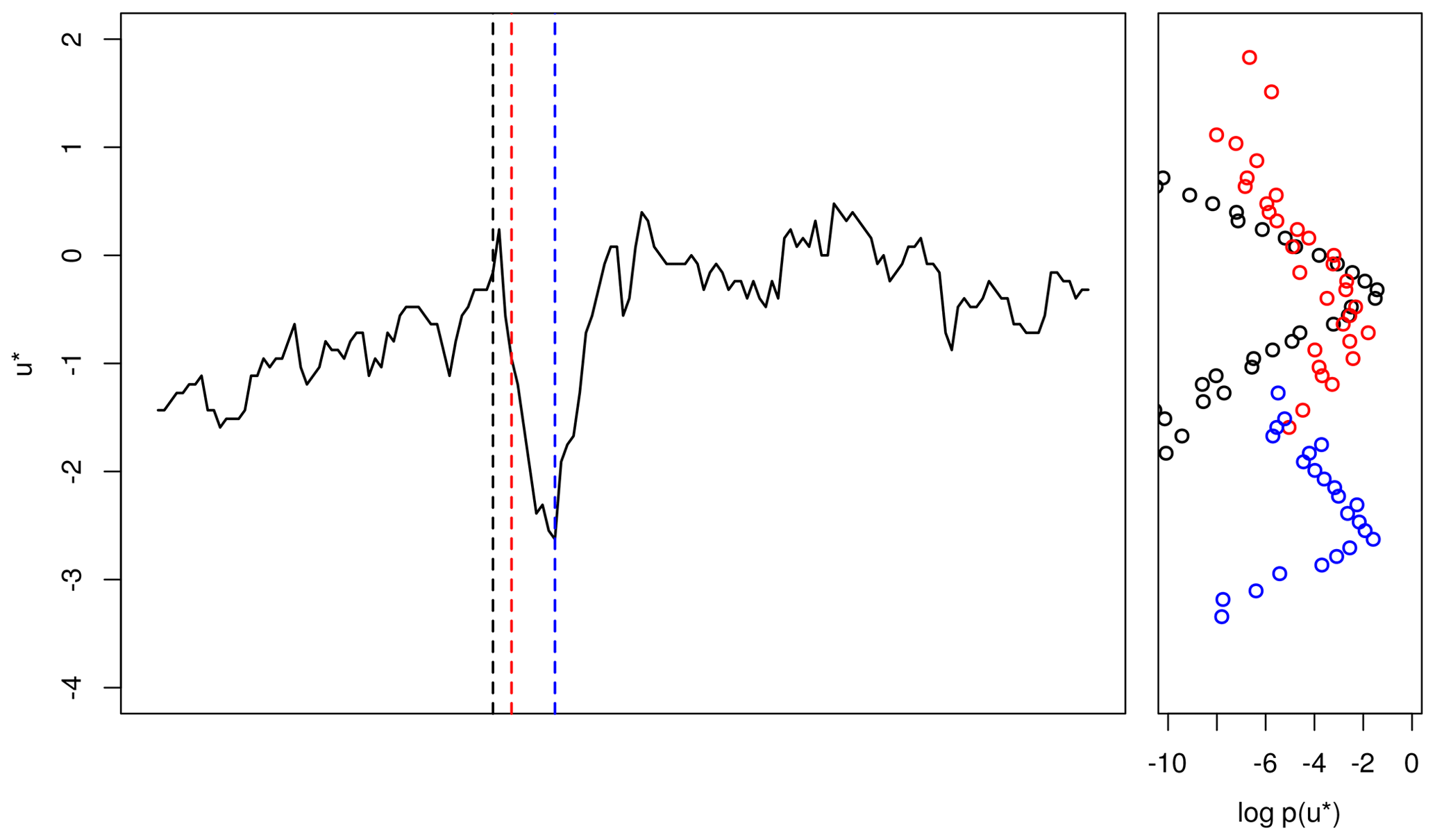
Figure 8Evolution of during reconstruction. Horizontal lines indicate snapshots of the pdf used for drawing the next sample of u*. The colours of the horizontal lines correspond to the snapshot pdf's.
In the preceding part for the reconstruction scheme, block-wise normalised wind speeds with a window length of 1 min were used. These blocks were defined by common mean wind speed and standard deviation σU. For the normalised wind speed u, we showed how to generate new time series; see Fig. 9.
There are different methods to generate more general non-stationary wind data. Knowing the slow variation in and σU(t), the drift and diffusion coefficients D(i) are taken as a slowly changing function of . If due to the normalisation of U to u the coefficients D(i) are in a good approximation independent of and σU, the slow variation in the real wind conditions can be incorporated over the back-transformation of the newly estimated values . The slow dynamics of and σU(t) may be given from measured data, meteorological simulations or other modelling.
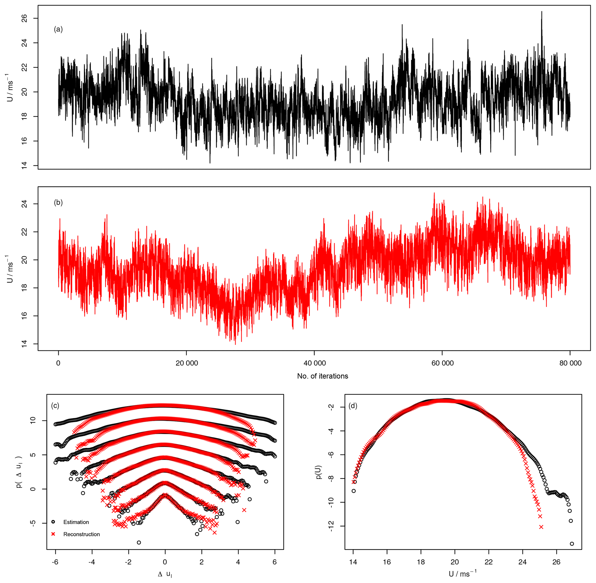
Figure 9(a, b) Comparison between measured non-stationary speeds U and reconstructed non-stationary wind speeds. (c, d) Increment and one point pdf's of original and reconstructed U.
A third possibility is a self-adaptive procedure which we show here. Instead of using given values of and σU(t), the intrinsic fluctuation of these quantities are used. Given an initial pair estimated over 1 min from measured data, a time series of non-stationary wind speeds U*(t) is obtained by applying the above-mentioned back-transformation to the generated wind speeds u* from our algorithm. For the upcoming simulation window of 1 min length, a new pair is estimated from the just generated block of wind speed data U*(t). This procedure is carried out until a time series of non-stationary wind speeds of desired length is obtained. In Fig. 9 such a time series is shown together with the statistical analysis of the increment pdf's and the marginal pdf of the non-stationary wind speed U. We observe that the pdf's of the reconstructed time series match the shape of the empirical pdf's for both the increments and the wind speeds. At this point we would like to emphasise that we do not aim to create copies of historical wind speeds, but rather to be able to generate stochastically equivalent time series.
We presented a stochastic approach based on multipoint statistics to generate surrogate short-time wind speed fluctuations with stochastic processes. Note these stochastic processes can be estimated self-consistently from given data. By using the normalised wind speeds u* and wind speed increments Δu(τi), Δu(τj) from two separate scales τi and τj, a three-point closure to the complex systems of wind speeds was achieved.
It was shown that our method works well in describing the dynamics of block-wise normalised wind speeds u* along scales τi in terms of a stochastic scale process, governed by a family of Fokker–Planck equations. This separation of the fluctuations from the mean values is similar to the Reynolds-averaged Navier–Stokes (RANS) approach widely used in fluid dynamics (Frisch, 2004), with the difference that we have a description of the underlying stochastic process of the fluctuation and “only” lack the mean values. With the modified reconstruction (see Sect. 3) we are able to generate mean values on the basis of past values of the reconstructed time series, yielding realistic non-stationary wind speed time series U*. As the typical response times of wind turbines and their control systems have duration of seconds to minutes, our reconstructed wind data are suitable for investigation of many dynamical effects of the wind energy conversion process. Note for these times the wind energy system may be driven into non-stationary response dynamics. Thus for these timescales it is important to have to maximal information on all statistical details of the driving wind source. The stochastic model presented here is based on multipoint statistics and is able to capture small-scale intermittency effects, extreme events and clustering of fluctuations, up to now not addressed in wind energy research.
For timescales larger than the response times of wind turbines, the turbines operate with fully adapted control systems in a stationary state. To estimate effects, like loads, of such stationary states, the temporal order of the states becomes unimportant. It is sufficient to know how often which wind situation emerges. Thus the knowledge of the valid Weibull distribution should be sufficient. Note our result here indicates that it would be better to extend the Weibull distribution to the joint probability .
Finally we emphasise that the presented stochastic multipoint approach to small-scale wind speed fluctuations should encompass automatically extreme short-term wind fluctuations, commonly added to wind investigations in terms of standard or multi-year gusts. These methods can be applied easily to other wind quantities like the temporal behaviour of shears, or wind veers, eventually combined in higher-dimensional stochastic processes (Siefert and Peinke, 2006). The results reported in Ali et al. (2019) show that such a stochastic modelling can also be used for wake flows.
To link Eq. (2) to the idea of an underlying turbulent cascade, we identify the conditional pdf on the left-hand side (lhs) with the cpdf . Thus the numerator of the right-hand side (rhs of Eq. 2) can be rewritten as
and the nominator as
The identity of the expressions in Eqs. (A1) and (A2) can mathematically rigorously be shown, as done in Nawroth et al. (2010), but intuitively speaking the sequences on the lhs and rhs must yield the same joint pdf, since the increments on the rhs have a common reference point u* or u1. Next we factorise the joint pdf's from Eqs. (A1) and (A2) by iteratively using cpdf's
and with with the timescale τi−τ1:
A further step in reducing the dimensionality of the involved pdf's can be performed upon assuming the scale process to be Markovian; i.e. there exists a timescale separation (j>i), where
holds. The timescale separation ΔτME is often called the Markov–Einstein length (Einstein, 1905), and for various systems its existence could be shown empirically, ranging from jet streams in laboratory experiments (Renner et al., 2001), (Reinke et al., 2018) to large geophysical systems such as ocean gravity waves (Hadjihosseini et al., 2016).
Data sets are available upon request by contacting the correspondence author.
CB did the preliminary analysis of the data, implemented the algorithms for the multiscale reconstruction and parametrization of the FPE, conducted all simulations, and wrote the main part of the manuscript. JP had the initial idea, and JP and MW supervised the work and helped in preparing the manuscript.
The authors declare that they have no conflict of interest.
The authors acknowledge helpful discussions with André Fuchs and Hauke Hähne.
This research has been supported by the VolkswagenStiftung (grant no. 8482) and by the Ministry for Science and Culture of the German Federal State of Lower Saxony (grant no. ZN3024, nieders. Vorab to M. W.).
This paper was edited by Horia Hangan and reviewed by two anonymous referees.
IEC: IEC 61400-1 Wind turbines Part 1: Design requirements, 2005. a
Ali, N., Fuchs, A., Neunaber, I., Peinke, J., and Cal, R. B.: Multi-scale/fractal processes in the wake of a wind turbine array boundary layer, J. Turbul., 20, 93–120, https://doi.org/10.1080/14685248.2019.1590584, 2019. a
Anvari, M., Lohmann, G., Wächter, M., Milan, P., Lorenz, E., Heinemann, D., Tabar, M. R. R., and Peinke, J.: Short term fluctuations of wind and solar power systems, New J. Phys., 18, 063027, https://doi.org/10.1088/1367-2630/18/6/063027, 2016. a
Boettcher, F., Renner, C., Waldl, H.-P., and Peinke, J.: On the statistics of wind gusts, Bound.-Lay. Meteorol., 108, 163–173, https://doi.org/10.1023/A:1023009722736, 2003. a, b
Brokish, K. and Kirtley, J. L.: Pitfalls of modeling wind power using Markov chains, in: 2009 IEEE/PES Power Systems Conference and 320 Exposition, 1–6, https://doi.org/10.1109/PSCE.2009.4840265, 2009. a, b
Carpinone, A., Langella, R., Testa, A., and Giorgio, M.: Very short-term probabilistic wind power forecasting based on Markov chain models, in: 2010 IEEE 11th International Conference on Probabilistic Methods Applied to Power Systems, 107–112, https://doi.org/10.1109/PMAPS.2010.5528983, 2010. a
Einstein, A.: Über die von der molekularkinetischen Theorie der Wärme geforderte Bewegung von in ruhenden Flüssigkeiten suspendierten Teilchen, Ann. Phys., 322, 549–560, https://doi.org/10.1002/andp.19053220806, 1905. a, b
Friedrich, R., Peinke, J., Sahimi, M., and Tabar, M. R. R.: Approaching complexity by stochastic methods: From biological systems to turbulence, Phys. Rep., 506, 87–162, https://doi.org/10.1016/j.physrep.2011.05.003, 2011. a
Frisch, U.: Turbulence: The Legacy of A. N. Kolmogorov, Cambridge University Press, Cambridge, https://doi.org/10.1017/CBO9781139170666, 1995. a, b
Hadjihoseini, A., Lind, P. G., Mori, N., Hoffmann, N. P., and Peinke, J.: Rogue waves and entropy consumption, EPL, 120, 30008, https://doi.org/10.1209/0295-5075/120/30008, 2018. a
Hadjihosseini, A., Wächter, M., P.Hoffmann, N., and Peinke, J.: Capturing rogue waves by multi-point statistics, New J. Phys., 18, 013017, https://doi.org/10.1088/1367-2630/18/1/013017, 2016. a, b, c, d
Haehne, H., Schottler, J., Waechter, M., Peinke, J., and Kamps, O.: The footprint of atmospheric turbulence in power grid frequency measurements, EPL, 121, 30001, https://doi.org/10.1209/0295-5075/121/30001, 2018. a
Kolmogorov, A. N.: A refinement of previous hypotheses concerning the local structure of turbulence in a viscous incompressible fluid at high Reynolds number, J. Fluid Mech., 13, 82–85, https://doi.org/10.1017/S0022112062000518, 1962. a
Milan, P., Wächter, M., and Peinke, J.: Turbulent Character of Wind Energy, Phys. Rev. Lett., 110, 138701, https://doi.org/10.1103/PhysRevLett.110.138701, 2013. a
Morales, A., Waechter, M., and Peinke, J.: Characterization of wind turbulence by higher-order statistics, Wind Energy, 15, 391–406, https://doi.org/10.1002/we.478, 2012. a
Mücke, T., Kleinhans, D., and Peinke, J.: Atmospheric turbulence and its influence on the alternating loads on wind turbines, Wind Energy, 14, 301–316, https://doi.org/10.1002/we.422, 2011. a
Nawroth, A. P. and Peinke, J.: Multiscale reconstruction of time series, Phys. Lett. A, 360, 234–237, https://doi.org/10.1016/j.physleta.2006.08.024, 2006. a
Nawroth, A. P., Friedrich, R., and Peinke, J.: Multi-scale description and prediction of financial time series, New J. Phys., 12, 083021, https://doi.org/10.1088/1367-2630/12/8/083021, 2010. a, b, c
Papaefthymiou, G. and Klockl, B.: MCMC for Wind Power Simulation, IEEE T. Energ. Convers., 23, 234–240, https://doi.org/10.1109/TEC.2007.914174, 2008. a
Peinke, J., Tabar, M. R., and Wächter, M.: The Fokker–Planck Approach to Complex Spatiotemporal Disordered Systems, Annu. Rev. Conden. Ma. P., 10, 107–132, https://doi.org/10.1146/annurev-conmatphys-033117-054252, 2019. a, b, c, d, e
Pesch, T., Schröders, S., Allelein, H. J., and Hake, J. F.: A new Markov-chain-related statistical approach for modelling synthetic wind power time series, New J. Phys., 17, 055001, https://doi.org/10.1088/1367-2630/17/5/055001, 2015. a
Reinke, N., Fuchs, A., Nickelsen, D., and Peinke, J.: On universal features of the turbulent cascade in terms of non-equilibrium thermodynamics, J. Fluid Mech., 848, 117–153, https://doi.org/10.1017/jfm.2018.360, 2018. a, b
Renner, C., Friedrich, R., and Peinke, J.: Experimental indications for Markov properties of small-scale turbulence, J. Fluid Mech., 433, 383–409, https://doi.org/10.1017/S0022112001003597, 2001. a, b
Risken, H.: The Fokker-Planck-Equation: Methods of Solution and Application, vol. 2 of Springer series in synergetics, Berlin, Springer, 1996. a, b, c
Siefert, M. and Peinke, J.: Joint multi-scale statistics of longitudinal and transversal increments in small-scale wake turbulence, J. Turbul., 7, N50, https://doi.org/10.1080/14685240600677673a, 2006. a
Stresing, R. and Peinke, J.: Towards a stochastic multi-point description of turbulence, New J. Phys., 12, 103046, https://doi.org/10.1088/1367-2630/12/10/103046, 2010. a, b, c
Wächter, M., Riess, F., Kantz, H., and Peinke, J.: Stochastic analysis of surface roughness, EPL, 64, 579–585, https://doi.org/10.1209/epl/i2003-00616-4, 2003. a
Wächter, M., Milan, P., Mücke, T., and Peinke, J.: Power performance of wind energy converters characterized as stochastic process: applications of the Langevin power curve, Wind Energy, 14, 711–717, https://doi.org/10.1002/we.453, 2011. a
Weber, J., Zachow, C., and Witthaut, D.: Modeling long correlation times using additive binary Markov chains: Applications to wind generation time series, Phys. Rev. E, 97, 032138, https://doi.org/10.1103/PhysRevE.97.032138, 2018. a
WindEurope: Wind in power 2017, available at: https://windeurope.org/wp-content/uploads/files/about-wind/statistics/WindEurope-Annual-Statistics-2017.pdf (last accessed: 18 August 2020), 2018. a