the Creative Commons Attribution 4.0 License.
the Creative Commons Attribution 4.0 License.
 | 08 Oct 2020
Lidar measurements of yawed-wind-turbine wakes: characterization and validation of analytical models
Mithu Debnath
Andrew Scholbrock
Paul Fleming
Patrick Moriarty
Eric Simley
David Jager
Jason Roadman
Mark Murphy
Haohua Zong
Fernando Porté-Agel
Wake measurements of a scanning Doppler lidar mounted on the nacelle of a full-scale wind turbine during a wake-steering experiment were used for the characterization of the wake flow, the evaluation of the wake-steering set-up, and the validation of analytical wake models. Inflow-scanning Doppler lidars, a meteorological mast, and the supervisory control and data acquisition (SCADA) system of the wind turbine complemented the set-up. Results from the wake-scanning Doppler lidar showed an increase in the wake deflection with the yaw angle and that the wake deflection was not in all cases beneficial for the power output of a downstream turbine due to a bias of the inflow wind direction perceived by the yawed wind turbine and the wake-steering design implemented. Both observations could be reproduced with an analytical model that was initialized with the inflow measurements. Error propagation from the inflow measurements that were used as model input and the power coefficient of a waked wind turbine contributed significantly to the model uncertainty. Lastly, the span-wise cross section of the wake was strongly affected by wind veer, masking the effects of the yawed wind turbine on the wake cross sections.
- Article
(7383 KB) - Full-text XML
- BibTeX
- EndNote


Wind turbines in wind farms can influence other turbines downstream and impact their performance. The interaction of the turbine rotor blades and the wind field creates a spatial volume of reduced wind speed and increased turbulence levels downstream of a wind turbine that can extend for several rotor diameters (Vermeer et al., 2003). This region is called the wake and affects downwind turbines negatively by decreasing power production and increasing fatigue loads (Thomsen and Sørensen, 1999). The spatial proximity of wind turbines in a wind farm and the wake effects on downwind turbines are important sources of power losses (Barthelmie et al., 2010). The magnitude of the power loss depends on wind direction, turbine spacing, wind speed, turbulence levels, and atmospheric stability (Stevens and Meneveau, 2017). In case of a fully waked wind turbine, losses around 40 % compared to a wind turbine in free flow have been observed (Barthelmie et al., 2010; Simley et al., 2020b).
Mitigating these wake effects on downwind turbines is an ongoing focus of research. Strategies that have been proposed are adjusting the blade pitch angle and the generator torque (Bitar and Seiler, 2013), counterrotating rows of wind turbines in wind farms (Vasel-Be-Hagh and Archer, 2017), optimizing the placement of the turbines within the wind farm based on terrain and wind climate (e.g. Shakoor et al., 2016; Kuo et al., 2016), or deflecting the wake away from the downwind turbine by introducing a yaw offset to the upwind turbine (Medici and Dahlberg, 2003). The latter approach, called wake steering or active yaw control, is the focus of this paper. It utilizes the thrust force that the rotor imposes on the flow, and, by offsetting the rotor from the flow direction, a transverse component of the thrust force is generated that displaces the wake from the line of the wind direction with the goal of deflecting it away from the downwind turbine. While the power production of the yawed turbine is reduced, this loss is potentially overcompensated for by the power gains of the downwind turbine (Bastankhah and Porté-Agel, 2015), and the strategy can be extended to a full wind farm (Gebraad et al., 2016). Wind tunnel studies of wake steering showed an increase in power for the combined upstream–downstream turbine pair between 3.5 % and 11 %, depending on inflow turbulence level and turbine separation distance (Bartl et al., 2018), and a field test at two commercial wind turbines showed an increase of 4 % (Fleming et al., 2019).
Analytical models describe the wake of a yawed wind turbine based on a set of turbine and inflow parameters (Jiménez et al., 2009; Bastankhah and Porté-Agel, 2016; Qian and Ishihara, 2018). These models are computationally cheap compared to numerical simulations and therefore can be used to find a set of yaw angles that maximizes the power output (Gebraad et al., 2016; Fleming et al., 2019). Validation of the analytical models for yawed-wind-turbine wakes and studies on the effectiveness of the wake steering have been done with wind tunnel experiments (e.g. Bastankhah and Porté-Agel, 2016) and numerical simulations (e.g. Vollmer et al., 2016). However, studies of yawed wind turbines using field data are rare: Fleming et al. (2017a) and Annoni et al. (2018) analysed the wake deflection, the wake recovery, and the power output for an isolated yawed turbine; Fleming et al. (2017b) investigated the effects of wake steering on the power production for a yawed upwind and a waked downwind turbine at a land-based site; Bromm et al. (2018) investigated the wake deflection of a yawed turbine with remote-sensing instruments with detailed error analysis; most recently Simley et al. (2020b) investigated the influence of the wind direction variability on the achieved yaw offsets and power gains based on the supervisory control and data acquisition (SCADA) data.
In this paper, field measurements, including inflow and wake measurements as well as SCADA data from a wake-steering upwind turbine and a waked downwind turbine, are used to (i) characterize the wake flow in terms of deflection, velocity deficit, and width; (ii) validate the wake deflection and power predicted from analytical models with the field measurements; and (iii) evaluate the wake-steering set-up implemented at this site.
This section introduces the measurement site, the instruments, the analytical models, and the data processing used to obtain the results. Indices are used to distinguish quantities measured by different instruments.
2.1 Research site and measurement set-up
The measurement site is a large wind farm in north-eastern Colorado, United States. Measurements were conducted at an isolated cluster of five turbines at the north-western edge of the wind farm from 23 December 2018 until 6 May 2019 with the set-up shown in Fig. 1. The area north of the turbines is flat grassland, and to the south and south-east is a downward-terrain step of approximately 150 m followed by flat grassland. The instruments measuring the inflow and the wake are introduced in Sect. 2.2. This article focuses on conditions with northern wind directions with flat grassland upwind and no structures or turbines affecting the inflow.
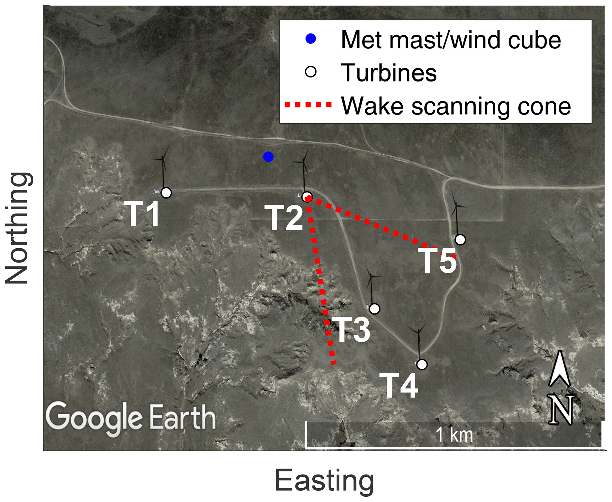
Figure 1Overview of the measurement site and set-up (© Google Earth). Shown in white are the five turbines of the local cluster, with the remainder of the wind park to the east. Turbine 2 (T2) was programmed to introduce a yaw offset if turbine 3 (T3) was downwind. The distance between T2 and T3 is approximately 390 m. T2 had two Doppler lidars installed on the nacelle to scan the inflow and the wake (Sect. 2.2.2 and 2.2.4). Shown in red is the scanning cone of the wake-scanning Doppler lidar for a case with the wind direction aligned with the direction to T3 and a yaw angle of 20∘. Shown in blue is the location of the meteorological mast and the WindCube (Sect. 2.2.3 and 2.2.1).
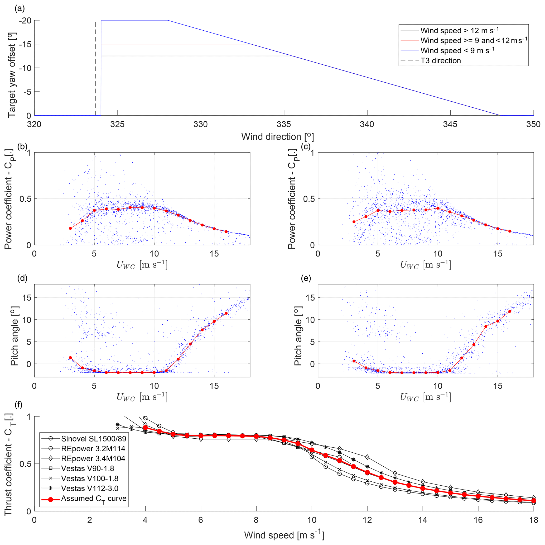
Figure 2Characteristics of the wind turbines used in the wake-steering experiment. Panel (a) shows the target yaw offset as a function of the wind speed and wind direction for T2. Panels (b) and (d) show the 30 min mean values (blue) and bin average (red) of the power coefficient and the blade pitch angle from the SCADA data of T2 as a function of the wind speed measured by the WindCube (Sect. 2.2.1). Panels (c) and (e) show the same for T3. Data from 6 January until 9 April 2019 are used in consistency with the results presented in Sect. 3. Panel (f) shows in black the thrust coefficient curves of six wind turbines from manufacturer data (first compiled by Abdulrahman, 2017) and in red the ensemble average assumed as the CT curve for T2.
The wind turbines were of the type 1.5sle from General Electric Energy, with active blade pitch control and a rated capacity of 1500 kW. Their hub height zhub is 80 m, and the rotor diameter D is 77 m. The SCADA data of T2 and T3 were provided by the wind park operator. T2 was equipped with a yaw controller to introduce a wind-speed-dependent yaw offset for wind direction between 324 and 348∘ to deflect the wake from T3 (Fig. 2a). The target yaw offset was pre-computed based on an optimization with an engineering model of wake steering as described in Fleming et al. (2019). A negative yaw offset is an anticlockwise rotation of the nacelle viewed from above. The power curve and pitch control of T2 are shown in Fig. 2b and d and for T3 in Fig. 2c and e. In absence of manufacturer information or measurement data for the thrust coefficient and due to the similarity of the thrust coefficient for most commercial wind turbines, the assumed thrust coefficient curve of the wind turbine follows the ensemble average shown in Fig. 2d. For a yawed turbine, the thrust coefficient is adapted with (Bastankhah and Porté-Agel, 2017), and the power coefficient is modified with (Adaramola and Krogstad, 2011), which includes the reduction in the rotor-swept area. The readings of the nacelle position in the SCADA data of T2 were incremented by 4∘ on 17 January 2019 without affecting the true nacelle position to remove a bias between the wind direction perceived by T2 and the WindCube. If the nacelle position of T2 is used to compute the position of T3 within the field of view of the wake-scanning lidar, this manipulation is reversed.
2.2 Measurement instruments
The instruments for the inflow and the wake measurements are introduced.
2.2.1 WindCube
A WindCube-V2 profiling Doppler lidar (manufactured by Leosphere and NRG Systems, Inc.) was located north-west of T2 and measured vertical profiles of the wind speed and the wind direction of the inflow (Fig. 1). The lidar uses a laser wavelength of 1.54 µm and internally computes the wind speed (UWC) and wind direction (dirWC) from a plan position indicator (PPI) scan with an azimuth step of 90∘ and an elevation angle of 62∘ followed by a vertical beam with the Doppler beam-swinging technique, assuming horizontal homogeneity (similar to the lidar in Lundquist et al., 2017). The measurement data were filtered with a signal-to-noise ratio (SNR) threshold of −22 dB. The WindCube was set-up to provide the vertical profiles from 40 to 260 m a.g.l. with a height resolution of 20 m and a sampling frequency of 1 Hz. The WindCube data are available from 6 January until 9 March 2019. Further, the yaw angle (γWC) can be computed from the difference between the wind direction at hub height and the nacelle position of T2.
2.2.2 WindIris
A WindIris Doppler lidar (manufactured by Avent Lidar Technology) was mounted on the nacelle of T2 and scans the inflow. The WindIris uses a four-beam geometry, with measurements at ±15∘ from the rotor axis in the horizontal direction and ±12.5∘ in the vertical direction. The WindIris provides the wind direction relative to the rotor axis (γWI), the wind speed (UWI), and the longitudinal turbulence intensity (TIWI) for an upwind distance of 50 to 200 m from the turbine and heights of 45 to 125 m a.g.l. Its measurements are within the induction zone of the turbine, and only vertically averaged measurements from an upwind distance of 90 m are used as a compromise between good data availability and a large upwind distance. The WindIris had problems that led to data loss during the campaign, which limits data availability to 12, 16, and 19 January and a long period from 24 January until 7 April 2019.
2.2.3 Meteorological mast
A meteorological mast was located north-west of T2, next to the WindCube. The wind direction from the wind vanes at 38 m a.g.l. (dirMM,38 m) and 56 m a.g.l. (dirMM,56 m), the wind speed of the ultrasonic anemometer at 50 m a.g.l. (USonic), and the wind speed of the cup anemometer at 60 m a.g.l. (UMM) are used. The wind vanes had an alignment issue until the week of 11 February 2019, when they were replaced with freshly calibrated units, and the cup anemometer had periods of suspicious measurements that might be connected to icing of the instrument. Further, the measurement data are not available for five periods during the campaign. For those reasons, the wind measurements from the meteorological mast are only used for validation of the WindCube. Further, the meteorological mast measured air temperature and air pressure near the surface, from which the density of dry air ρMM is computed.
2.2.4 Stream Line
A Stream Line Doppler lidar (manufactured by Halo Photonics Ltd.) was mounted on the nacelle of T2, scanning the wake downwind of the turbine. It performed an hourly scan schedule consisting of 2D and 3D scans of the wind field downwind. The 2D scans were horizontal swipes at an elevation of 0∘ and covering an azimuth range from 160 to 220∘, with an azimuth step of 1.5∘ (Fig. 3a). These swipes were repeated 53 times back and forth within a 28 min period. The 3D scans consisted of PPI swipes at nine elevation angles, which were repeated between 20 and 22 times within a 31 min period. The 3D scan pattern was iterated throughout the campaign with changes to the covered azimuth range and positions of the elevation levels (compare Fig. 3b and c). These changes were made to capture the wake at short downwind distances but have little effect on the measurements of the wake flow at the position of the downwind turbine. Further, other scan patterns were introduced to the scan schedule during the campaign, but those are not used in this study. The Stream Line system had an azimuth misalignment from the rotor axis of −0.15∘ after installation on the nacelle. Levelling of the instrument is affected by tower movements, but their effects on the beam positions are mitigated by a grid-based post-processing of the measurement data introduced in the following section.
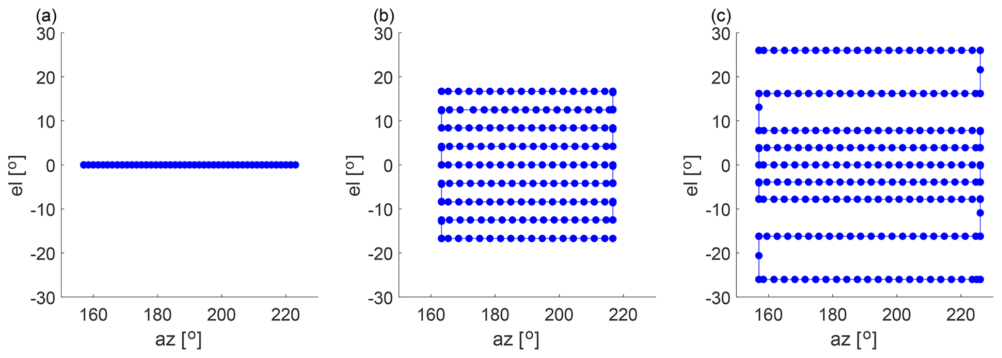
Figure 3The scan pattern of the 2D (a) and the 3D scans with equally spaced elevation levels (b) and elevation levels with larger spacing at the top and bottom (c). The path of the scanner is shown as a blue line, with measurement points indicated as blue points.
2.3 Data processing
The processing of the measurement data is introduced in the order in which it was done to obtain the results.
2.3.1 Inflow measurements and data selection
The 10 and 30 min mean values and standard deviations of the wind speed, wind direction, and yaw angle were computed from the data of the WindCube, WindIris, meteorological mast, and SCADA data. A filter was used to identify suitable intervals for further processing of the wake-scanning lidar. The filter criteria are as follows:
-
Data are available for the WindCube, the WindIris, and the SCADA data of T2 and T3.
-
Wind speed from the WindCube and WindIris is between 4 and 15 m s−1.
-
Neither T2 nor T3 had a downtime, and the rotor was turning.
-
The 10 min period comprising a 30 min period had changes of less than 3 m s−1 for the wind speed and less than 5∘ for the wind direction
Further, the 30 min periods had to satisfy one of the two following conditions to be classified as either a wake-steering case or a control case.
-
Wake-steering cases: north-western inflow with the WindCube wind direction between 320 and 350∘, active yaw control of T2 (compare Fig. 2a), and the mean yaw angle between 3 and 30∘ for both WindIris and WindCube;
-
Control cases: north to north-eastern inflow with the WindCube wind direction between 0 and 75∘ and the yaw angle between −3 and 3∘ for both WindIris and WindCube
The processing of the wake-scanning Stream Line Doppler lidar described in the next section was carried out for periods that satisfied the above filtering criteria. Periods were rejected at later stages if the measurements of the Stream Line system were not available or if the SNR filter rejected measurements in the investigated scan area. Because the selection of suitable periods described here is based on 30 min periods, but the 2D and the 3D scans of the Stream Line Doppler lidar were 28 and 31 min long, respectively, the final inflow parameters used for the results were recomputed for the precise scan durations at a later stage.
2.3.2 Processing of wake-scanning Doppler lidar data
For the suitable periods identified in the previous section, the data of the wake-scanning Stream Line system were processed according to the following steps:
-
An SNR filter with a threshold of −17 dB was applied to remove low-quality data points. If the mean SNR at hub height was too low at a distance of 4 D, the scan was rejected altogether (e.g. periods with aerosol-free air or fog).
-
The azimuth angle of each lidar beam was adjusted so that the measurements were fixed in space relative to the ground by removing changes in the nacelle position recorded in the SCADA data. The transformation is given by
where azwsl,i is the azimuth angle of the ith beam during the scan, azSC,i is the nacelle position of T2 at the time of the measurement, and is the angular mean nacelle position for the scan duration. A rejection of periods with excessive nacelle position changes was not necessary because the stationariness criterion of the wind direction in the previous section already removed periods with large changes in the nacelle position.
-
The measurements were rotated into the mean wind direction such that it aligned with az=180∘ of the wake-scanning lidar with
-
The radial velocity measured by the Doppler lidar was transformed to the longitudinal velocity based on elevation and azimuth angles, sorted into a regular spherical coordinate system, and interpolated on a Cartesian coordinate system with 10 m resolution. These procedures are described in Fuertes et al. (2018) for the 2D scans and in Brugger et al. (2019) for the 3D scans.
The above steps provided the longitudinal mean velocity field u2D(x, y) and u3D(x, y, z) in a Cartesian right-hand system with its origin at the nacelle of T2 and the x axis pointing in the wind direction and the z axis pointing upward. The corresponding velocity deficits are then given by
and
with uWC(z) interpolated to the grid heights.
2.3.3 Wake deflection from the wake-scanning Doppler lidar
The wake was characterized by fitting a Gaussian function given by
to , y) and , y, zhub) at each downwind distance. The fit used a Gaussian weighting function with a width of 1.5σ. The position of the peak given by δ(x) is equivalent to the wake deflection because the coordinate system was rotated into the wind direction (Eq. 2). To remove cases where the Gaussian fit was influenced by the wakes or the hard targets of neighbouring turbines and to ensure that only results within the far wake are used, the result was rejected if the correlation coefficient of the Gaussian fit and the measurement data were below 0.99 at (a visual verification showed that all instances of this problem were detected).
2.3.4 Power and rotor-averaged velocity from the Doppler lidars
The power of the upwind turbine (T2) was computed from the inflow measurements of the WindCube with the assumption that the inflow is horizontally homogeneous across the rotor area. It is then given by
with the rotor area A defined by D, and CP,T2 was interpolated from the power curve of T2 shown in Fig. 2 based on the UWC(zhub). For the downwind turbine (T3), the power was computed from the longitudinal velocity field of the wake-scanning lidar by integration over the rotor area. It is given by
with D and yT3 the transverse position of T3 in the coordinate system aligned with the wind direction. The integrals were approximated by sums according to the grid resolution of the measurement data. The power coefficient was interpolated from the power curve of T3 based on the average velocity across the rotor area for T3 given by
with D and the bar indicating a mean value. The power that T3 would have produced for a non-yawed T2, , is estimated from the wake-scanning lidar with Eq. (7) and D under the assumption that yawing affects primarily the spatial position of the wake, and effects on the shape of the wake are minor.
2.4 Analytical models
Three analytical models are compared with the field measurements for validation of the models themselves and to investigate the efficiency of the wake-steering set-up. The analytical models were introduced by Jiménez et al. (2009), Bastankhah and Porté-Agel (2016), and Qian and Ishihara (2018), respectively, and their equations are presented in Appendix A. All three models use the longitudinal turbulence intensity of the WindIris, the average yaw angle of the WindIris and the WindCube, and the thrust coefficient as input variables and predict the longitudinal velocity deficit field Δumod(x, y, z) of the wake. The thrust coefficient is interpolated from the assumed thrust curve in Fig. 2f with the wind speed of the WindCube. The models are computed for each investigated 30 min period separately with the same 10 m resolution Cartesian coordinate system as the velocity fields of the wake-scanning lidar for consistency. Together with the inflow measurements of the WindCube, the longitudinal velocity field is computed with
where uWC(z) is interpolated to the grid levels. The model prediction for the rotor-averaged velocity and the turbine power of T3, Pmod and Umod, is then computed from the model analogous to Eqs. (7) and (8) but with the predicted longitudinal velocity field of the analytical model instead of the velocity field from the lidar measurements. The power of T3 for a hypothetically non-yawed T3, , is estimated by computing the model with γ=0∘. However, umod(x, y, z) cannot be evaluated at downstream distances shorter than the predicted onset of the far wake. This can become a problem with the short turbine spacing of the measurement site for cases with very low turbulence intensities of the inflow, and these cases are discarded from the results where appropriate.
The analysed time frame is from 6 January until 9 April 2019 because, outside of that time frame, data of either the WindIris or the WindCube were missing. The synoptic conditions were characterized by the winter season with daily mean temperatures mostly between −10 and 5 ∘C. The main wind directions were north-west and south-east, with wind speeds up to 25 m s−1 (Fig. 4).
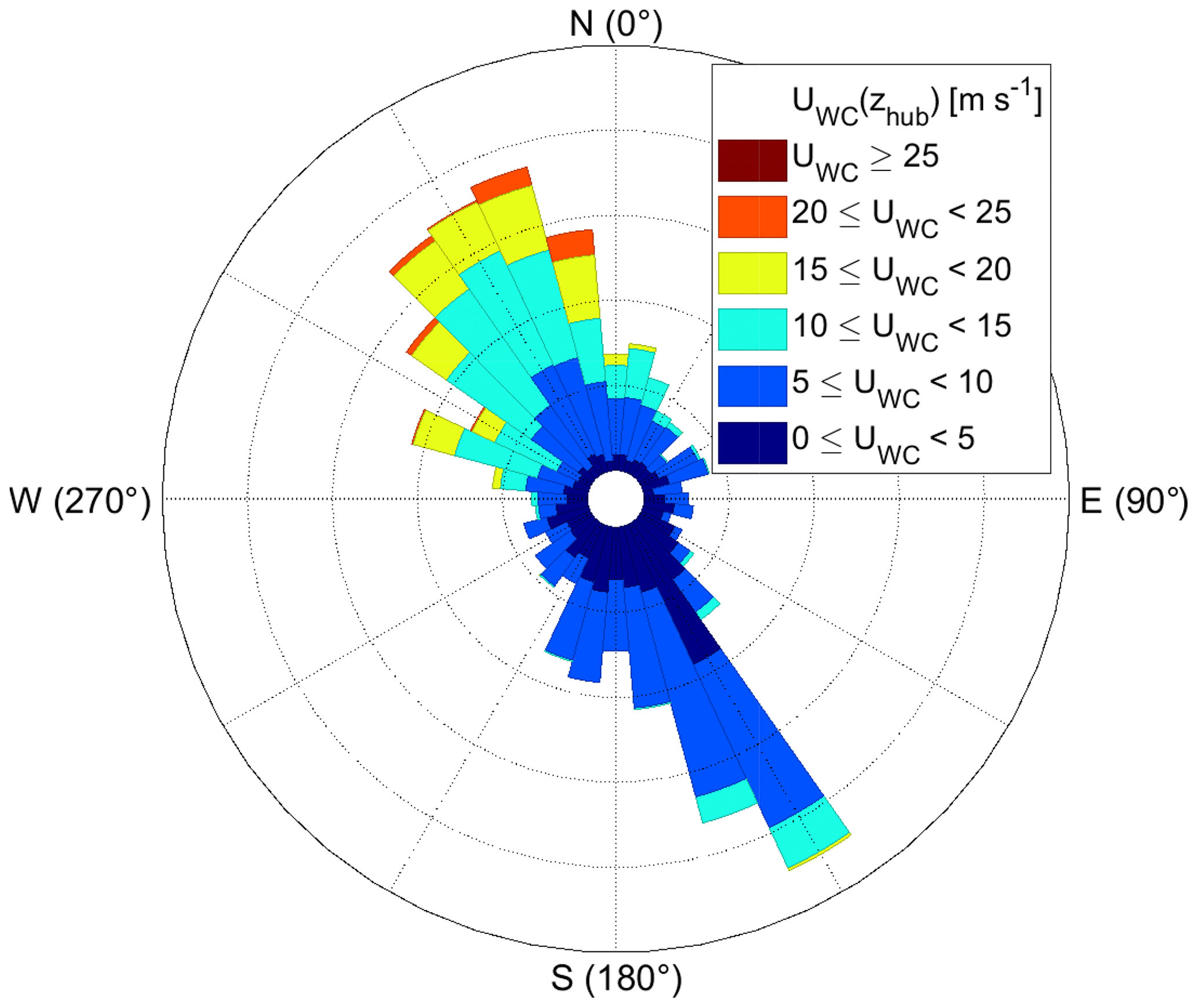
Figure 4Wind rose based on the uWC and dirWC at hub height using the full data set from 6 January until 9 April 2019. Software written by Daniel Pereira was used to create the wind rose (https://www.mathworks.com/matlabcentral/fileexchange/47248-wind-rose, last access: 11 December 2019, MATLAB Central File Exchange).
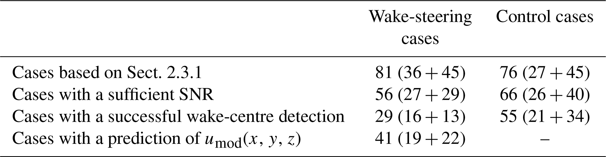
The results presented in the following are based on the wake-steering cases and the control cases as defined in Sect. 2.3.1 (with the exception of Sect 3.4.1). Table 1 presents a summary of the available cases. Periods of clear air and snow or fog events reduced the SNR of the wake-scanning lidar and its data availability. Further, the detection of the wake deflection or the prediction of umod(x, y, z) failed for some cases, which are discarded where necessary.
Table 1Overview of wake-steering cases (middle column) and control cases (right column). From top to bottom: the number of 30 min periods that met the requirements of Sect. 2.3.1, the number of cases with a sufficient SNR of the wake-scanning lidar, the number of cases with a successful detection of the wake centre based on the correlation threshold (Sect. 2.3.3), and the number of cases for which the model prediction of umod(x, y, z) was possible (Sect. 2.4). The numbers outside of the brackets are the total cases, and the numbers inside the brackets are the 2D scans and 3D scans of the wake-scanning lidar, respectively.
3.1 Inflow
The inflow measurements, especially of the yaw angle, are essential for the quality of the results presented in the following sections. Therefore, an inter-comparison of the inflow measurements for wind speed, wind direction, and yaw angle are presented.
The wind speeds from the WindCube, ultrasonic anemometer, cup anemometer, and WindIris are compared in Fig. 5. The WindCube shows good agreement to the ultrasonic anemometer, with a slight underestimation by the ultrasonic anemometer at high wind speeds, which might be explained by the height difference (Fig. 5a). The agreement between the WindCube and the cup anemometer is also good, with a slope near unity and a small underestimation by the cup anemometer (Fig. 5b). The WindCube and the WindIris show systematic deviations due to the induction zone of the wind turbine (Fig. 5c). Based on this comparison, the wind speed of the WindCube is used in the following because it is available at hub height, not influenced by the induction zone, and compares well with the ultrasonic and cup anemometer.
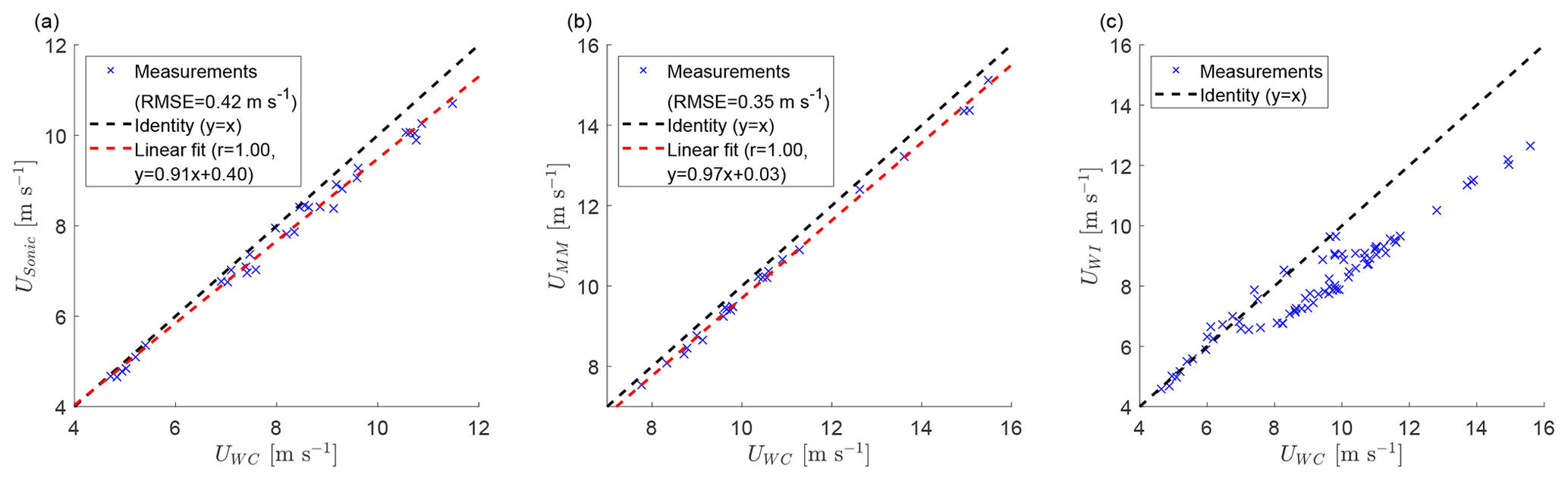
Figure 5Inter-comparison of the inflow wind speed measurements between the ultrasonic anemometer at 50 m and the WindCube at 60 m (a), the meteorological mast at 60 m and the WindCube at 60 m (b), and the WindIris and the WindCube at hub height (c) using the wake-steering and the control cases. Measurement data of the ultrasonic anemometer and the cup anemometer were not available for all cases. The dashed black line shows the identity x=y, and a linear fit is shown as a dashed red line together with the correlation coefficient r.
The wind direction from the WindCube and the two wind vanes of the meteorological mast have a large offset to each other until a 5 d maintenance starting on 11 February 2019. Therefore, only the wake-steering and the control cases after 16 February 2019 are used for the wind direction comparison (Fig. 6). The RMSEs of 1.36∘ for the lower wind vane and 2.64∘ for the upper wind vane include contributions from a remaining bias between WindCube and wind vanes. If the bias is removed, the RMSE reduces to 1.23 and 1.61∘, respectively. The findings for the yaw angle shown in the next paragraph suggest that the WindCube has a correct north alignment. As for the wind speed, the WindCube is used as reference for the wind direction because it agrees with the meteorological mast after its maintenance, so it was presumably also correct before.
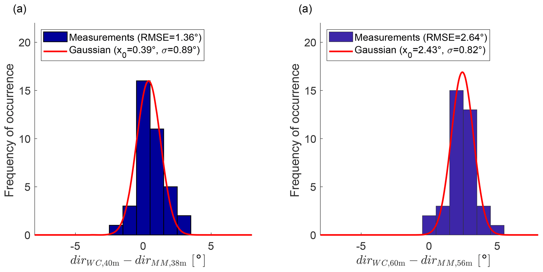
Figure 6Histogram of the wind direction difference between the WindCube and the meteorological mast for 40 m a.g.l. (a) and 60 m a.g.l. (b) using the wake-steering and the control cases after 16 February 2019 (the wind vanes on the meteorological mast were misaligned before 16 February 2019). The red line shows a Gaussian fit to the histogram.
The yaw angle from the WindIris, the SCADA data, and the WindCube are compared (Fig. 7). The data-filtering criteria of Sect. 2.3.1 were applied without the yaw angle restriction for the control cases because it would artificially reduce the measurement errors. For the non-yawed control cases, the yaw angle of the SCADA data and the WindCube have a similar RMSE with the WindIris and a bias of less than 1∘ (Fig. 7a and c). For the wake-steering cases, a large bias between the WindIris and the SCADA data can be seen for ∘ (Fig. 7b) that is not present between the WindCube and the WindIris (Fig. 7d). This is reflected in a doubling of the RMSE between the WindIris and the SCADA data from the control cases to the wake-steering cases, while the RMSE between the WindCube and the WindIris increased only slightly. This observation suggests that yawing of the wind turbine affects the measurements of the wind vane on top of the nacelle.
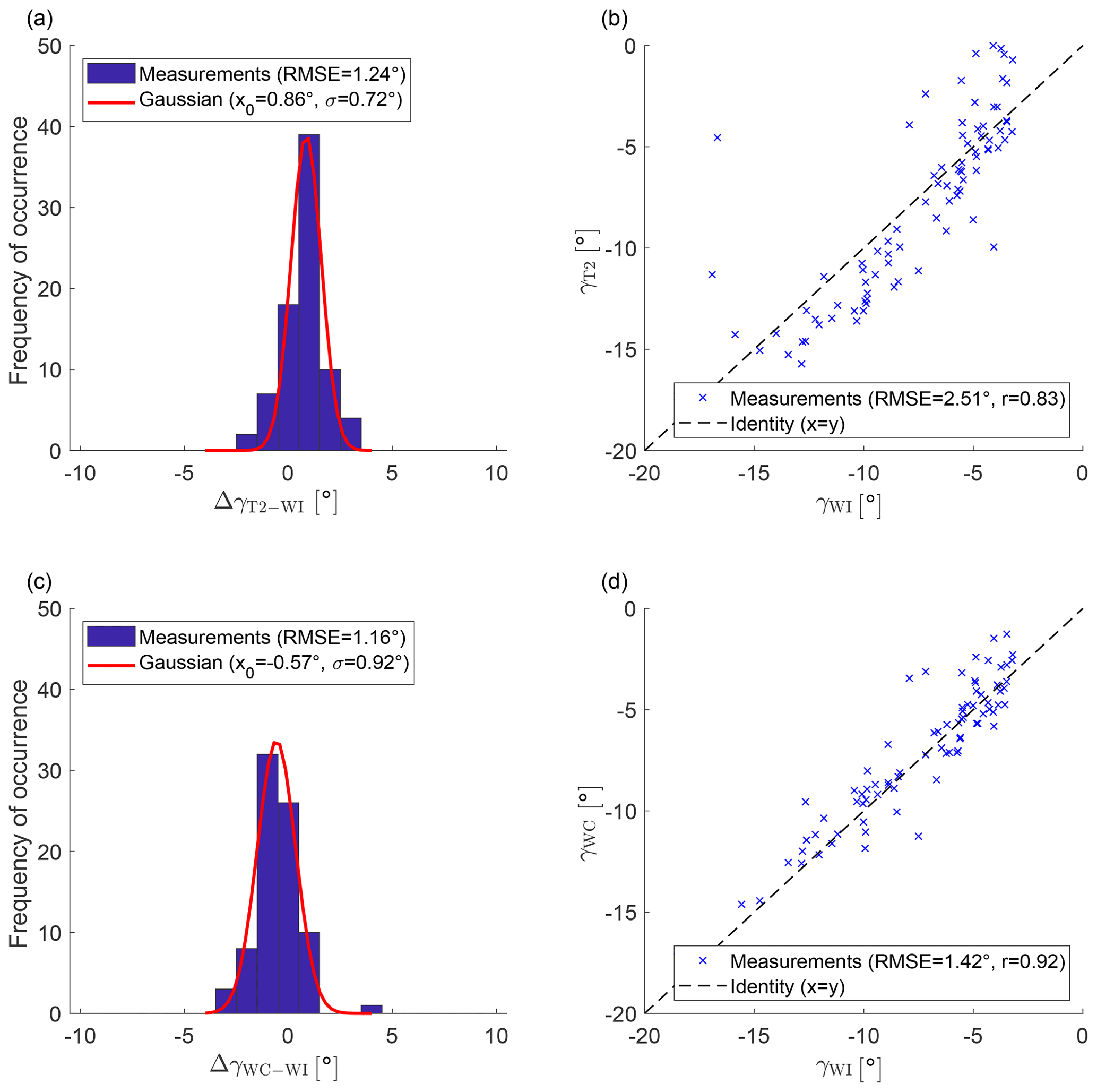
Figure 7Inter-comparison of the yaw angle measurements. Panel (a) shows a histogram of the yaw angle difference between the WindIris and the SCADA data of T2 for the control cases. Panel (b) shows the yaw angle from the SCADA data of T2 and the WindIris for wake-steering cases. Panel (c) shows a histogram of the yaw angle difference between the WindCube and the WindIris for the control cases. Panel (d) shows the yaw angle from the SCADA data of T2 and the WindIris for wake-steering cases. The red line shows a Gaussian fit to the histogram, and the dashed black line is the identity. The data were filtered according to Sect. 2.3.1, but for (a) and (c) the yaw angle limitation was omitted.
3.2 Wake deflection
Before investigating the wake deflection caused by the wake steering, the wake deflection is verified for the non-yawed control cases, where no wake deflection is expected (Fig. 8). Based on the RMSE found for the yaw angle (Fig. 7c and d), the expected RMSE of the wake deflection should be between and . This is the case for the for the WindIris (Fig. 8a) and the WindCube (Fig. 8b). Further, both distributions have a mean value that is not significantly different from 0. The consistency between the yaw angle errors and the wake deflection distribution shows that the wake scanning and its spatial positioning were working well. The absence of a bias shows that the alignment of the wake-scanning lidar with the rotor axis is correct (the measured offset of 0.15∘ during the installation was taken into account in the processing). Because the yaw angle and the wake deflection provided by the WindIris and the WindCube are of comparable quality, the yaw angle, γ, used in the remainder of the article is the average of both.

Figure 8Histograms of the normalized wake deflection δ∕D at for the control cases with a successful wake-centre detection. Panel (a) shows the normalized wake deflection based on the yaw angle from the WindIris (γWI) and (b) for the yaw angle of the WindCube (γWC). Both 2D and 3D scans of wake-scanning lidar for control cases with a successfully detected wake centre are used.
The deflection of the wake centre from the downwind direction due to wake steering is investigated next, starting with a discussion of the example case shown in Fig. 9a. This case was selected because it has the largest yaw offset of all wake-steering cases, which makes the wake deflection easy to visually observe in the mean longitudinal velocity field. The wake-centre detection was successful around , but the non-Gaussian shape of the near wake and neighbouring wind turbine wakes led to problems at other downwind distances, which were detected and rejected with the correlation threshold (Sect. 2.3.3). The analytical models were computed from the inflow measurements taken at the same time as the example case as described in Sect. 2.4 and are also shown in Fig. 9a. The Bastankhah and Porté-Agel (2016) model and Qian and Ishihara (2018) model show visually good agreement with the observed wake deflection, but the Jiménez et al. (2009) model overestimates it. These qualitative observations from this example case are extended to all wake-steering cases in the following.
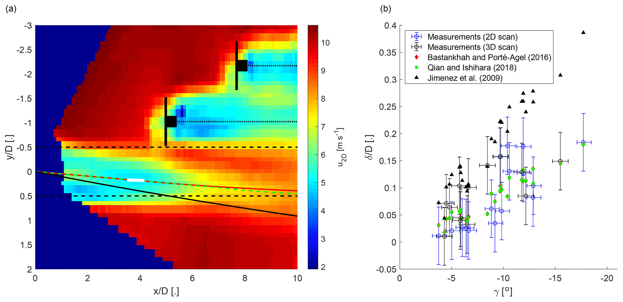
Figure 9Panel (a) shows an example from the wake-steering cases with a mean yaw offset of γ=18∘. The mean longitudinal velocity field is shown as a colour image. The predicted wake deflection of the Bastankhah and Porté-Agel (2016) model is shown as a solid red line, the Qian and Ishihara (2018) model is shown as a dashed green line, and the Jiménez et al. (2009) model is shown as a solid black line. The solid white line shows the result of the wake-centre detection with a correlation coefficient larger than 0.99 (see Sect. 2.3.3). The dashed black line indicates the rotor area of T2. Turbines 3 and 4 are stylized in black, and a dotted black line is a visual aid to indicate the downwind direction. Panel (b) shows the normalized wake deflection at as a function of the yaw angle for the wake-steering cases with a successful wake detection and a model prediction at . The measurements are shown in blue for the 2D scans and in black for the 3D scans. The error bars are based on the errors found between WindIris and WindCube (Sect. 3.1). The analytical models of Jiménez et al. (2009; black triangles, Eq. A25), Bastankhah and Porté-Agel et al. (2016; red diamonds, Eq. A7), and Qian and Ishihara (2018; green squares, Eq. A18) are plotted for each case.
The wake deflection at a downwind distance of is shown in Fig. 9b for all wake-steering cases with a successful wake-centre detection. The observed wake deflection increases with the yaw angle as expected from wind tunnel experiments (Bastankhah and Porté-Agel, 2016) and numerical simulations (Lin and Porté-Agel, 2019). The analytical model of Jiménez et al. (2009) overestimates the wake deflection, and the models by Bastankhah and Porté-Agel (2016) and Qian and Ishihara (2018) better match the wake deflection from the field measurements. The overestimation of the Jiménez et al. (2009) model was also observed by Bastankhah and Porté-Agel (2016) with wind tunnel experiments and by Lin and Porté-Agel (2019) with numerical simulations. The measurement data show considerably larger scattering than the model predictions, which is likely a consequence of the remaining non-stationarity of the atmospheric boundary layer in the data set and the measurement errors of the yaw angle. It should be noted that the short downwind distance of at which the models are evaluated is heavily influenced by the wake skew angle assumed for the near wake, which is used to provide an initial condition for the far wake. The similar wake deflections for the Bastankhah and Porté-Agel (2016) model and the Qian and Ishihara (2018) model are then explained by the identical wake skew angle used by both models (Eqs. 10 and 22), and noticeable differences of the wake deflection between these two models only appear at larger x∕D.
3.3 Power
The velocity fields predicted by the analytical models and measured by the Doppler lidars are used to estimate the power of the wind turbines. First, the power estimated from the Doppler lidars is compared with the SCADA data. Afterwards, the predictions of the three analytical models are validated against the SCADA data and the measurements of the wake-scanning lidar. The investigation is carried out for the wake-steering cases with a 3D scan of the wake-scanning lidar and a model prediction at (Table 1).
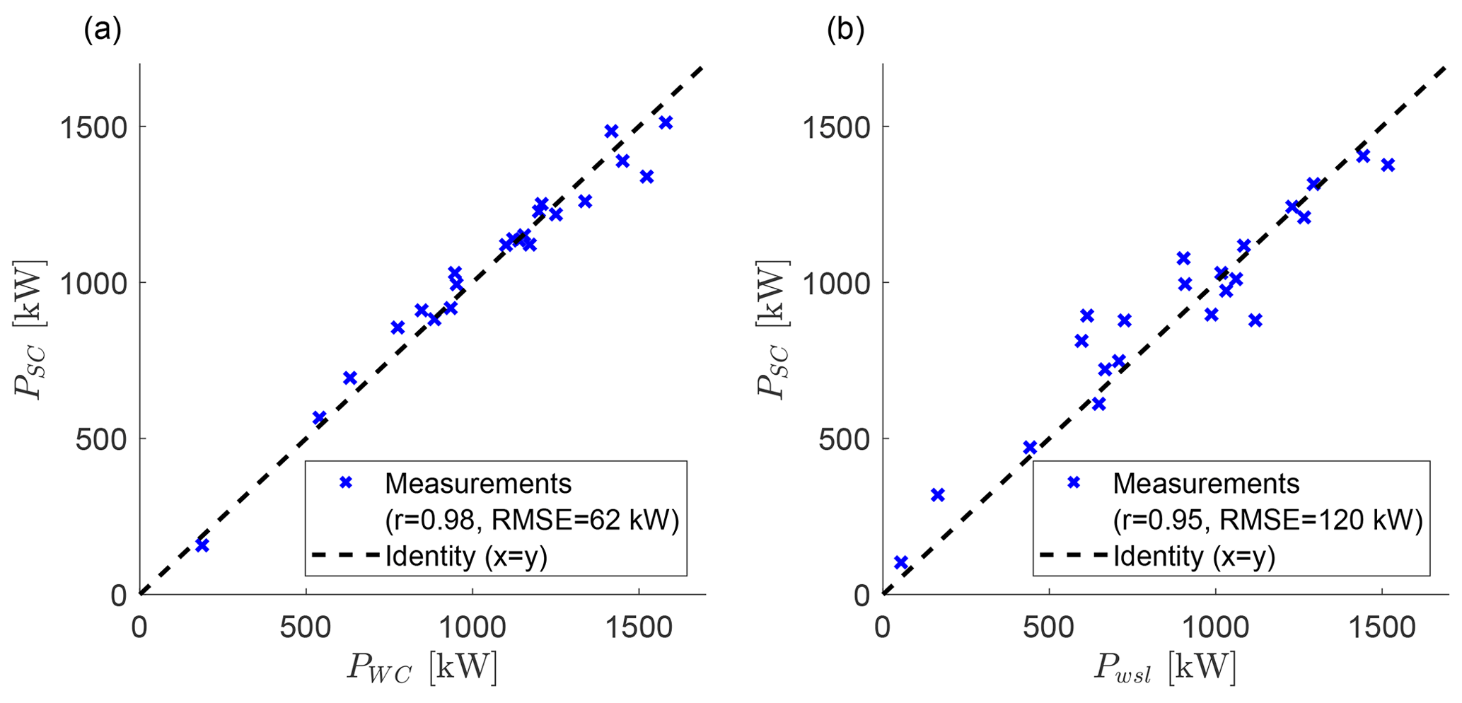
Figure 10Comparison of the power from the SCADA data and the power estimated from the Doppler lidar measurements for T2 (a) and T3 (b) using the wake-steering cases with a 3D scan of wake-scanning lidar and a model prediction at . Blue crosses show the measurement data, and the dashed black line is the identity (y=x).
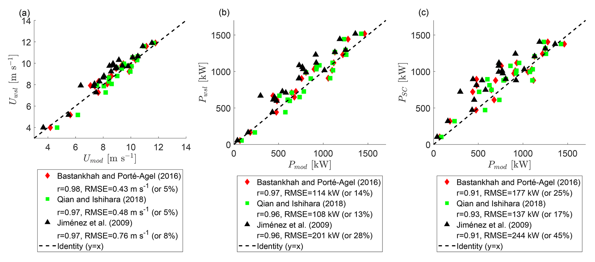
Figure 11The rotor-averaged velocity prediction of the analytical models for T3 compared with the measurements by wake-scanning lidar (a). The power prediction of the analytical models for T3 compared with the wake-scanning lidar (b) and the SCADA data (c). Data of the wake-steering cases with a 3D scan of wake-scanning lidar and a model prediction at are used. Red diamonds show the Bastankhah and Porté-Agel (2016) model, green squares show the Qian and Ishihara (2018) model, black triangles show the Jiménez et al. (2009) model, and the dashed black line is the identity.
3.3.1 Estimated power from the Doppler lidars
The power estimated from the measurements of the Doppler lidars (Eqs. 6 and 7) is compared with the SCADA data. The power of T2 from the WindCube and the SCADA data (Fig. 10a) has better agreement than the power of T3 from the wake-scanning lidar and the SCADA data (Fig. 10b). A possible reason for the larger errors for T3 could be that the specification of the power coefficient is problematic for a waked wind turbine because T3 is usually waked by T2 for the wake-steering cases. The differences between the wake-scanning lidar and the WindCube are less likely to be an explanation because the wake-scanning lidar has a higher measurement density across the rotor area and a more favourable scan geometry. The power differences between the WindCube and the SCADA data show no relationship to the yaw angle (not shown), indicating that the adjustment of the power coefficient of a yawed turbine with cos 3γ holds for the field data.
3.3.2 Model validation for the power
The model validation is carried out in three steps to distinguish various error contributions, starting with a comparison of the rotor-averaged velocity of T3 from the Bastankhah and Porté-Agel (2016) model, the Qian and Ishihara (2018) model, and the Jiménez et al. (2009) model with the measurements of the wake-scanning lidar (Fig. 11a). The Qian and Ishihara (2018) model and the Bastankhah and Porté-Agel (2016) model both have an error of 5 %. The Jiménez et al. (2009) model has a considerably larger error than the other two models because it assumes a top-hat velocity deficit that overestimated the velocity deficit at the edges of the wake, which resulted in an underestimation of the rotor-averaged velocity for a partially waked downwind turbine. The Gaussian velocity deficits of the other two models better matched the Doppler lidar observations in this respect. The model input values are subject to measurement errors, which propagated into an uncertainty of the model error. This uncertainty is estimated by varying the model input values based on the errors found in Sect. 3.1. The error propagation of γ and TIWI introduces an uncertainty of less than 0.5 %, while the error propagation of uWC and dirWC had an effect of 2 % and 1 %, respectively.
A comparison of the power of T3 from the analytical models with the wake-scanning lidar is shown in Fig. 11b. The increased error percentages compared to the rotor-averaged velocity in Fig. 11a are explained by the error magnification due to the cubed velocity in the computation of the power.
A further increase in the error is observed if the analytical models are combined with the power curve of the wind turbine for comparison with the SCADA data (Fig. 11c). This is in line with the assumption from the previous section that the specification of the power coefficient is problematic for waked wind turbines. Using different methods to estimate the power coefficient does not affect the overall findings (e.g. using the velocity in front of the nacelle instead of averaging the rotor area or switching between the model prediction and the lidar measurement). The average error propagation from the WindCube measurements is estimated to be 52 kW, which roughly agrees with the error between the power estimated from the WindCube and the SCADA data of T2 (Fig. 10a) and highlights the fact that the found errors are not only due to the models but include significant contributions from the measurement errors.
3.4 Effect of wake steering on the power
The effect of wake steering on the power of the downwind turbine (T3) and the full system of upwind and downwind turbines (T2 + T3) is first investigated with a case study and afterwards using the wake-steering cases with a 3D scan of the wake-scanning lidar and a model prediction at (Table 1).
3.4.1 Case study of the wake steering
The data set is searched for pairs of 30 min periods with T3 downwind of T2 and similar inflow conditions but one being yawed and the other not. All periods where the wind direction was aligned with the downwind turbine within 1∘ were ordered by the wind speed, and two suitable pairs were identified (Fig. 12a and b). In the case of the second pair, the turbulence intensity was too low for the analytical model to make a prediction at , and therefore only the first pair is discussed in the following.

Figure 12The inflow wind speed (a), the yaw angle of T2 (b), and the power (c) for all 30 min periods with the wind direction aligned with the downwind turbine within 1∘ sorted by wind speed (data filtering of Sect. 2.3.1 not applied). Highlighted with circles are the two pairs with similar wind speed and wind direction and all measurement data available but different yaw angles. The two bottom panels show the mean longitudinal velocity fields at hub height from the wake-scanning Doppler lidar for the first pair with the non-yawed case (d) and the yawed case (e). The rotor area shadow of T2 is indicated as a dashed black line, and the position of T3 is stylized in black.
The inflow measurements and the power output of the turbines of the example case are summarized in Table 2a, and the longitudinal mean velocity fields of the wake-scanning lidar are shown in Fig. 12d and e. The increase in wind speed together with the power losses of the yawed turbine could explain the power increase for T2 from the yawed to the non-yawed case seen in the SCADA data. For T3, the SCADA data report higher power for the case with wake steering compared to the case without wake steering, which could be explained by the deflection of the wake.
Table 2Inflow and power output for the yawed case (left column) and non-yawed case (right column) shown in Fig. 12d and e. The upper part (a) presents the inflow measurement from the Doppler lidars and power from the SCADA data. The lower three parts show the power estimated from the inflow-profiling lidar for T2 and the prediction of the Qian and Ishihara (2018) model for T3 based on the inflow values (b), the averaged inflow values only varying γ (c) and the inflow values with γ=0 (d).
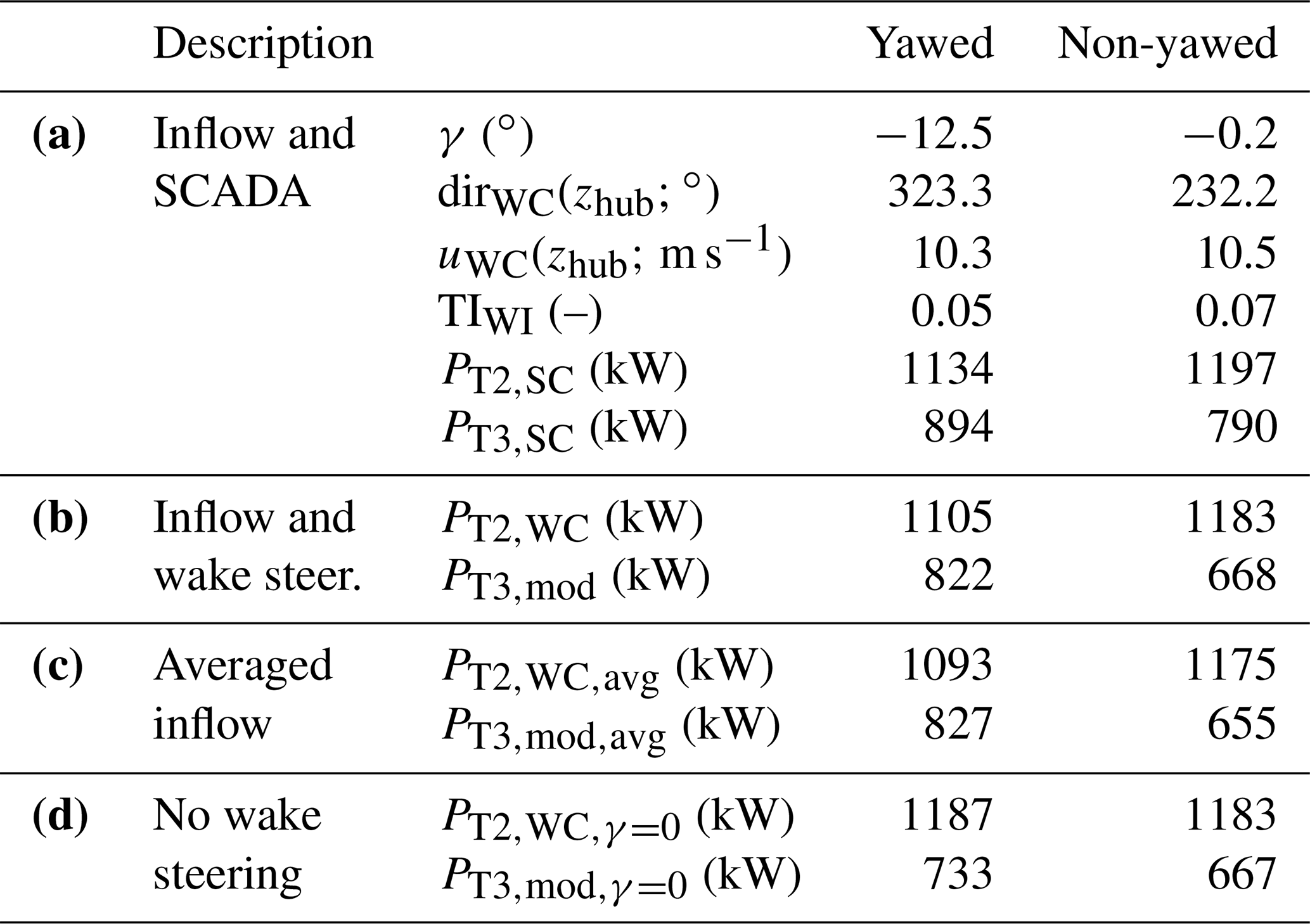
Using the Qian and Ishihara (2018) model and the inflow measurements to predict the power of the turbines captures the tendencies but underestimates the power for T3 (Table 2b). The effect of the wake steering can be isolated by averaging TIWI and uWC(z) for both cases and only varying γ (Table 2c). Conversely, the effect of the inflow conditions can be isolated by setting γ=0∘ and using TIWI and uWC(z) as measured (Table 2d). The results show that the wake steering had an effect on the power of T3, and changes in the inflow alone cannot explain the power differences between the yawed and the non-yawed case. Based on the analytical model and the SCADA data, the yawed T2 lost 60–80 kW, and T3 gained 90–170 kW by the wake steering. As a side note, it was observed that wake steering is not necessary at high wind speeds because the wake has enough available power for the downwind turbine to run at its rated capacity (Fig. 12c).
Using yawed and non-yawed cases with similar inflow conditions as above to investigate the effect of wake steering for a wider part of the data set is not feasible due to the limited number of suitable pairs. However, this example case illustrated that using an analytical model to artificially remove the wake steering captures the power changes and can be used to investigate the effect of wake steering on the power.
3.4.2 Wake-steering evaluation
The effect of wake steering on the power is investigated using the periods classified as wake-steering cases. The data for 12 and 24 January 2019 have been excluded from this part of the analysis because the yaw controller had toggling issues. The data set is divided into two groups based on the wind direction following a visual inspection of the volumetric lidar measurements, which showed two categories of wake-steering cases:
-
successful wake steering, where the wake of the yawed T2 was partially or completely deflected away from T3 (Fig. 13a and b);
-
unnecessary or harmful wake steering, where the wake of the yawed T2 would have missed T3 even if T2 would not have yawed (Fig. 13c and d) or where the wake of the yawed T2 was deflected towards T3 instead of away (Fig. 13e and f).
Geometrical considerations of the rotor area shadow of T2 in the wind direction can explain the unnecessary cases. The harmful wake-steering cases were observed for wind directions very close to or smaller than the direction toward T3 and might be explained by the bias of the wind direction perceived by the wind turbine under yawed conditions (Fig. 7b) or the variability of the wind direction during the scan period (Simley et al., 2020a). Therefore, the effect of wake steering is investigated separately for a subgroup with a narrow inflow sector from 325 to 335∘ in addition to all wake-steering cases.
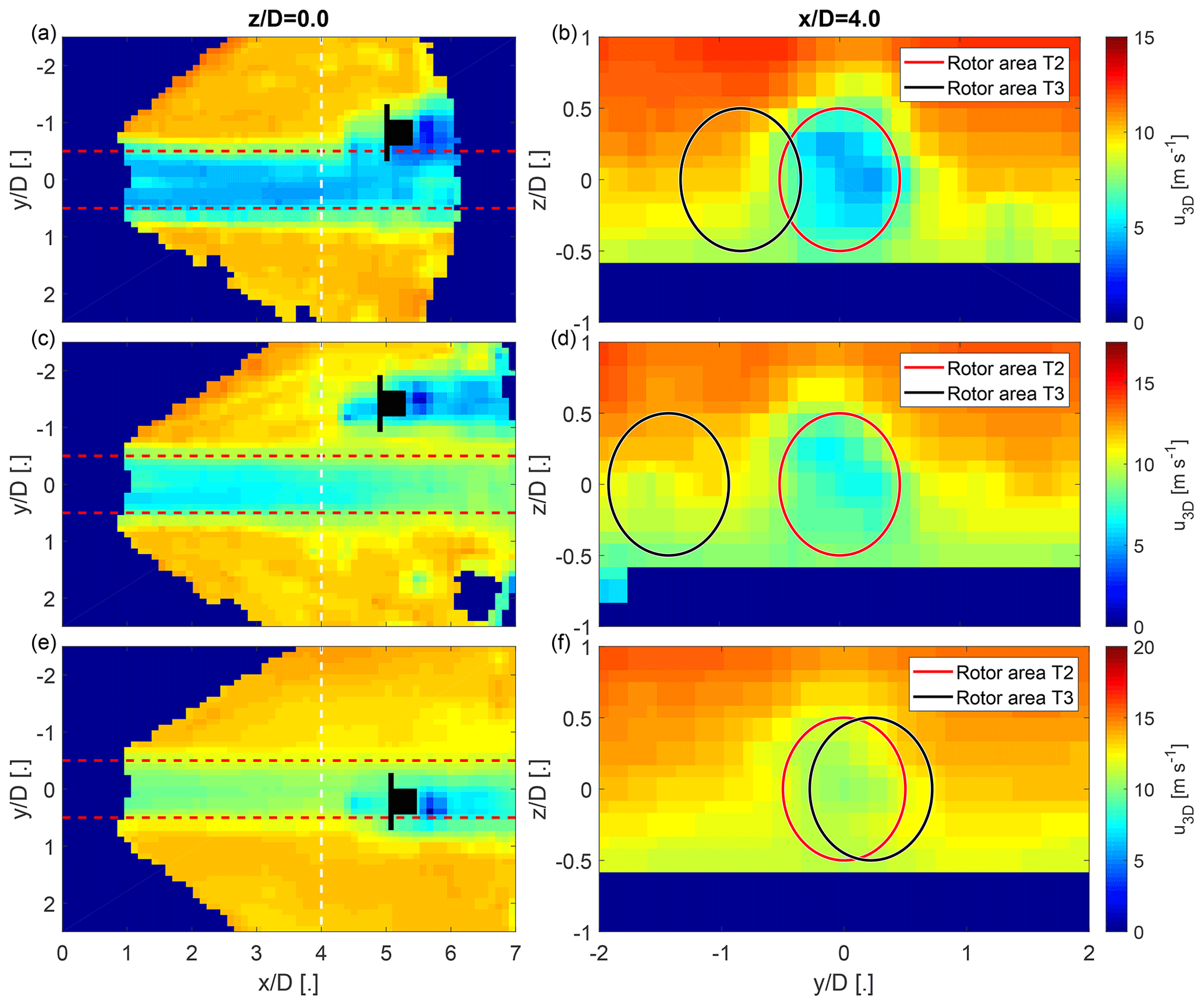
Figure 13Three examples selected from the wake-steering cases to illustrate successful and detrimental cases of wake-steering. Panels (a) and (b) show a successful wake-steering case. Panels (c) and (d) show an unnecessary wake-steering case. Panels (e) and (f) show a harmful wake-steering case. The colour scale shows the longitudinal velocity of the wake-scanning Doppler lidar. The left column shows a horizontal cross section of the longitudinal velocity at hub height. The right column shows span-wise cross sections of the longitudinal velocity at a downwind distance of 4 D. The dashed red lines and solid red circles show the outline of the rotor area of T2 in wind direction. The position of T3 is stylized in black, and the solid black circle shows the rotor area of T3.
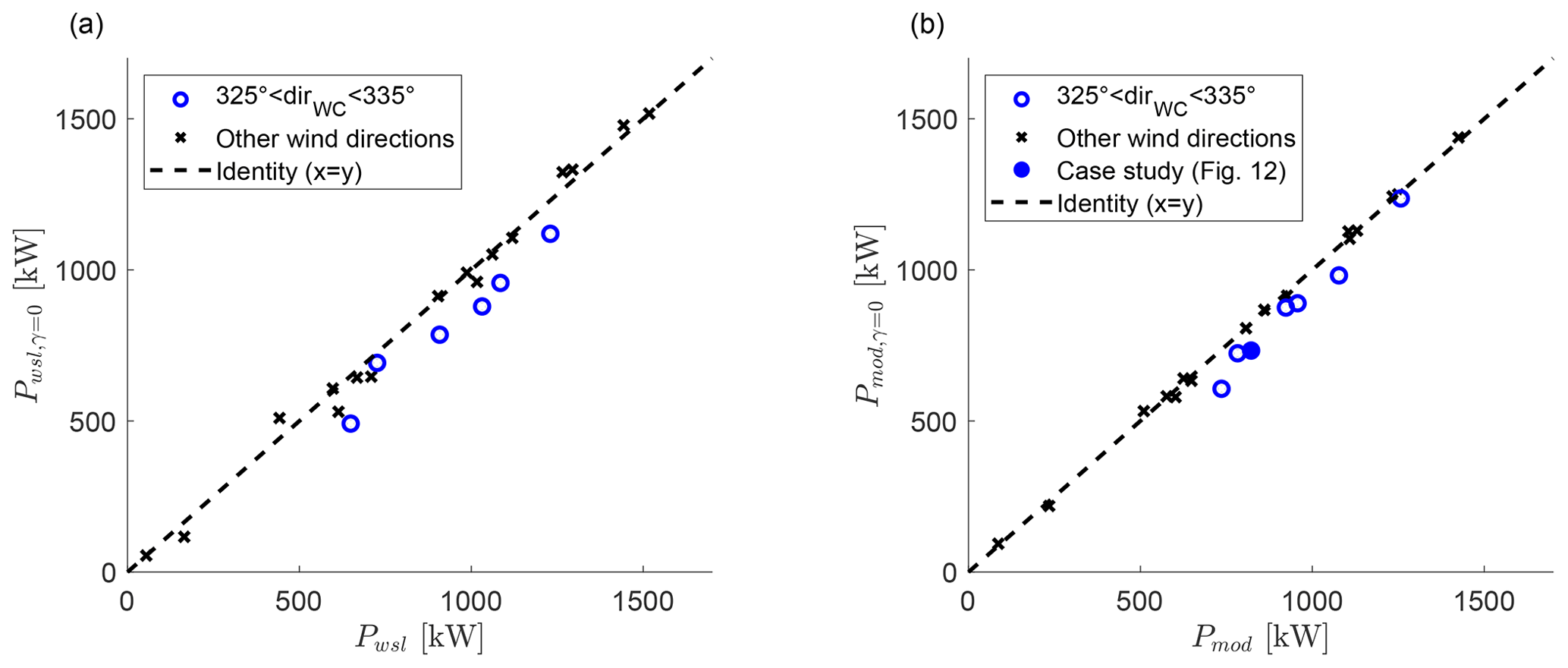
Figure 14The effect of wake steering on the power of the downstream turbine (T3) based on the wake-scanning lidar (a) and the Qian and Ishihara (2018) model (b). Data of the wake-steering cases with a 3D scan of wake-scanning lidar and a model prediction at are used. The hollow blue circles indicate data points from the narrow inflow sector, the black crosses are data points outside of the narrow inflow sector, and the solid blue circle is the yawed example case from Fig. 12.
Table 3Maximum and average power gains and losses due to wake steering for the subgroup with wind directions between 325 and 335∘ and considering all wind directions. The two left columns show the power changes based on the wake-scanning lidar; the two right columns show the power changes based on the Qian and Ishihara (2018) model. The results of the downwind turbine (T3) and the combined system of upwind and downwind turbines (T2 + T3) are shown for both. The percentage values are based on the power of the yawed case. Data of the wake-steering cases with a 3D scan of wake-scanning lidar and a model prediction at are used.
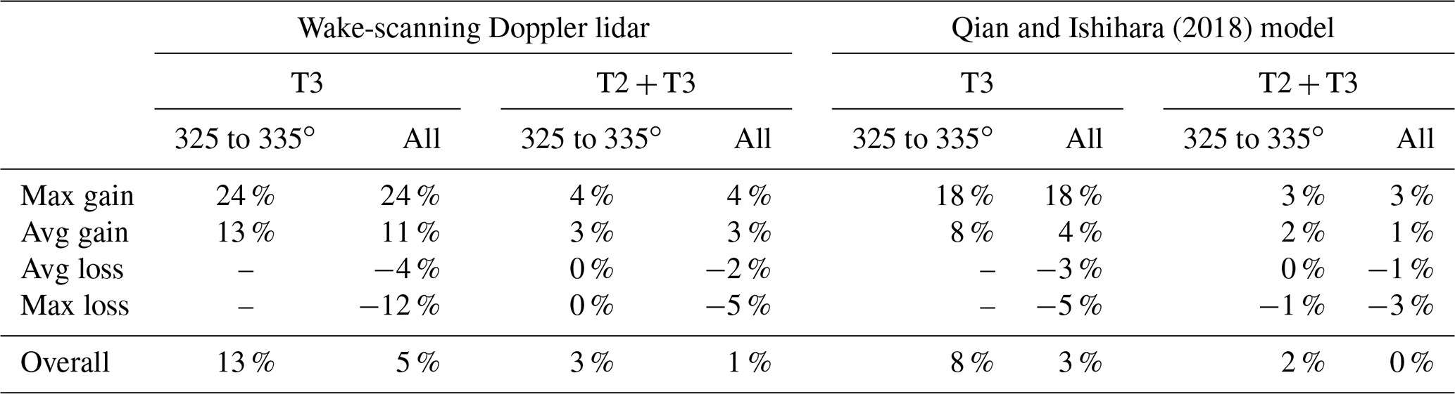
The effect of wake steering on the power of the downstream turbine (T3) is investigated based on the wake-scanning lidar (Sect. 2.3.4) and based on the Qian and Ishihara (2018) model (Sect. 2.4). The results in Fig. 14 show a power increase for T3 for the cases with a wind direction between 325 and 335∘, but the cases outside of this wind direction range have very small power gains or even power losses. Table 3 summarizes these findings and also includes the power gains of the combined system of upstream and downstream turbines. The combined system that includes the power losses of the yawed upstream turbine (T2) has a power improvement of 2 %–3 % for the narrow wind direction sector but shows virtually no improvement for the wider wind direction sector. The harmful or unnecessary wake-steering cases were reducing the power gains significantly for the wake-steering set-up in this study. These findings are in line with the findings of Simley et al. (2020b) using a SCADA data-driven approach.
Field measurements of yawed-wind-turbine wakes were performed with a nacelle-mounted scanning Doppler lidar. The wake was characterized in terms of depth, width, and deflection from planar and volumetric scans of the Doppler lidar. Together with the inflow measurements, these data were used for validation of three analytical wake models and evaluation of the wake-steering set-up.
The observed wake deflection increased with the yaw angle, and the comparison to the analytical models showed an overestimation by the Jiménez et al. (2009) model, while the Bastankhah and Porté-Agel (2016) model and the Qian and Ishihara (2018) model matched the measurement data better. The predictions of the Qian and Ishihara (2018) model and the Bastankhah and Porté-Agel (2016) model for the rotor-averaged velocity of the downstream turbine had errors of 5 %, while the Jiménez et al. (2009) model had considerably larger errors. These model errors include the error propagation from the inflow measurements that are used as input for the analytical models. Power predictions using the analytical models had an error magnification due to the cubed velocity in the computation of the power. Further, the specification of the power coefficient for the calculation of the power output from the waked wind turbine was shown to be a problematic issue.
The wake steering in this set-up was not working optimally, with some cases even being detrimental to the power output. The wake-scanning lidar and the Qian and Ishihara (2018) model both showed that the wake was not always deflected away from the downwind turbine. The combination of the bias of the wind vane on top of the nacelle when the turbine was yawed, the variability of the wind direction within the averaging period, and the implemented wake-steering design could explain those cases. Narrowing the wind direction range for which a yaw offset is applied mitigated those problems to some extent but is not an optimal solution. Especially the bias of the wind vane when the turbine is yawed should receive further attention because it could result from a flow distortion in the proximity of the nacelle during yawed operation, which would point to a problem of the standard wind turbine instrumentation providing the input measurements for the wake steering with the needed quality. It might be possible to correct this bias in the yaw controller with a turbine-specific correction function if it only depends on the yaw angle and the wind speed. A forward-facing Doppler lidar could solve this problem, and it could also open up the possibility for measurements of the incoming turbulence level. Using an external wind direction measurement like the WindCube in this study is problematic for large wind farms due to the horizontal homogeneity assumption.
Application of analytical models to predict the power of waked downstream turbines would benefit from a power coefficient adapted to an inhomogeneous wind field across the rotor area and an improved description of the near wake for better handling of short turbine spacing or low turbulence intensities. A kidney shape of the wake cross section was not observed, which is likely explained by the dominant effect of the wind veer on the span-wise shape of the wake (Appendix B). Non-stationarity of the boundary layer, which cannot be handled by the analytical model, was the most limiting factor in the selection of suitable periods for the validation.
The equations of the three analytical models compared in this article are summarized from their respective publication for convenience.
A1 Bastankhah and Porté-Agel (2016)
The analytical model from Bastankhah and Porté-Agel (2016) is based on the conservation of momentum and assumes a Gaussian distribution of the velocity deficit. The wake skew angle in the near wake is given by
with γ given in radians. The length of the near wake is given by
with α=2.32 and β=0.154. The width of the wake in the far wake (x≥x0) is given by
for the vertical direction and by
for the transversal direction. The wake growth rate is assumed to be isotropic in the span-wise plane and proportional to the turbulence intensity with
following the results of a field campaign (Fuertes et al., 2018). For TIx<0.06, the wake growth rates are set to 0.021 to account for the turbulence induced by the turbine itself. The wake deflection from the line of wind direction at the onset of the far wake is given by
and for the far wake (x≥x0) by
with
and
Lastly, the velocity deficit is computed with
A2 Qian and Ishihara (2018)
The model of Qian and Ishihara (2018) also uses a Gaussian distribution of the velocity deficit. The different definition of the thrust coefficient used in Qian and Ishihara (2018) is related to the definition employed here by . The wake growth rate is given by
and the potential wake width at the rotor plane is given by
The wake skew angle in the near wake is given by
and the wake width at the onset of the far wake is given by
with the near wake length given by
The wake growth in the far wake is given by
and the wake deflection at the onset of the far wake is given by
The deflection of the wake centre from the line of wind direction is given by integration of the wake skew angle in the downwind direction (Howland et al., 2016) with
with
and
The normalized velocity deficit is given by
with
and
A3 Jimenez et al. (2009)
The analytical model of Jiménez et al. (2009) is also based on the conversation of momentum but assumes a top-hat distribution of the longitudinal velocity deficit. The wake growth rate is given by Eq. (A11), and the wake skew angle is given by
Integration of the wake skew angle in a downwind direction provides the wake deflection, which is given by
The normalized velocity deficit is given by
for and 0 outside. Other methods to compute the velocity deficit based on a top-hat distribution found in the literature were tested but resulted in larger errors (Peña et al., 2016; Frandsen et al., 2006).
The kidney-shaped span-wise cross sections of yawed-turbine wakes observed in wind tunnel experiments (Bastankhah and Porté-Agel, 2016) and numerical simulations (Howland et al., 2016; Lin and Porté-Agel, 2019) were not observed in the data from the field measurements. Using the point vortex transportation model introduced by Zong and Porté-Agel (2020), it is shown that the effect of wind veer, which is frequently present in the atmospheric boundary layer, has a dominant effect on the shape of the wake. Even without wind veer, yaw angles smaller than 20∘ have a small effect on the shape of the wake that could be missed with the wake-scanning lidar. The strong effect of wind veer is in line with a simple assessment of the wake displacement based on the transversal advection due to the wind veer with
with a wind veer of ∘ across the rotor area. It provides for the bottom and top tips at (Abkar et al., 2018). The effect of wind veer is not further analysed here because it has already been studied from field measurements in Bodini et al. (2017) and Brugger et al. (2019).
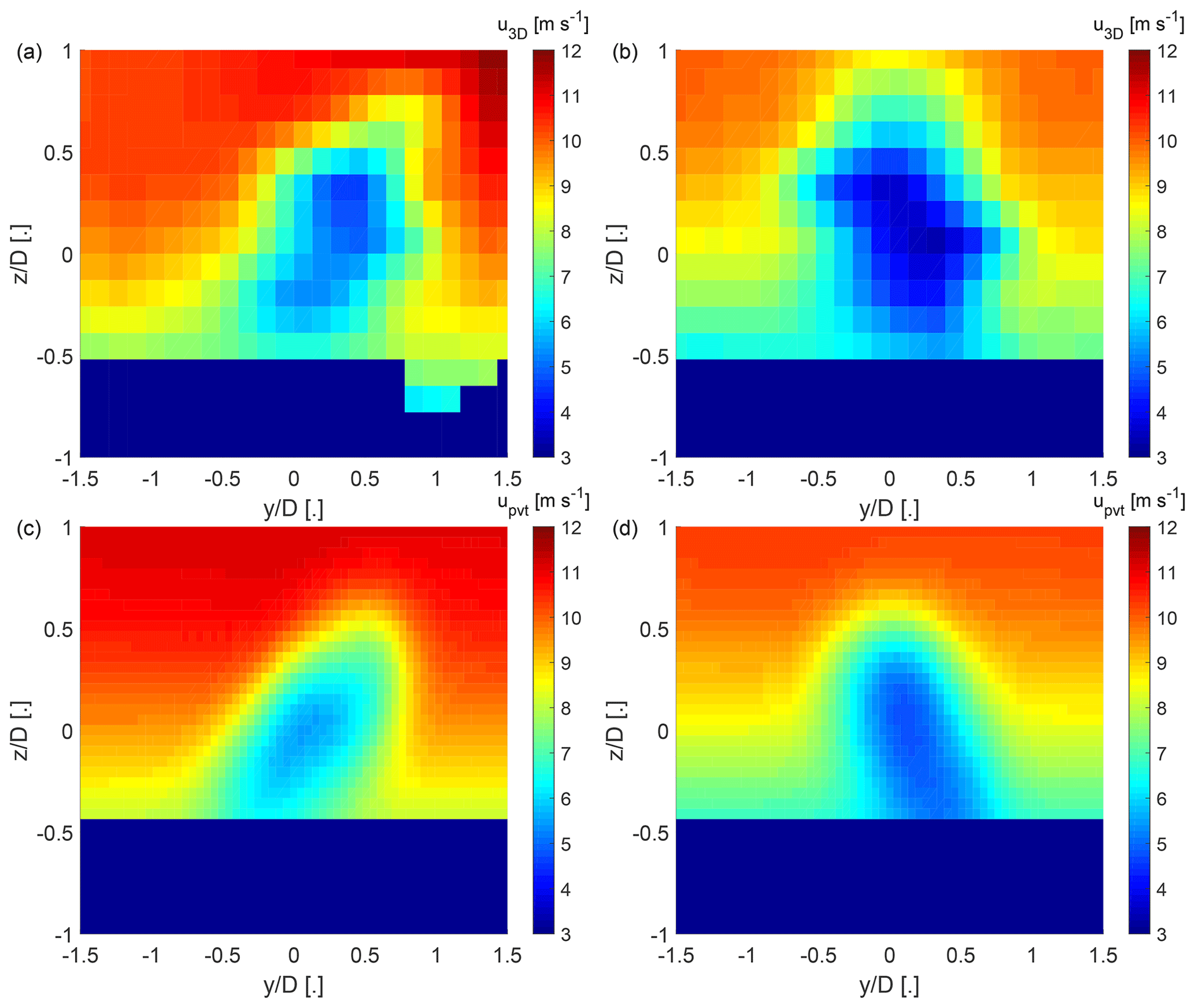
Figure B1Span-wise cross sections of the longitudinal velocity field at . Panels (a) and (b) show the velocity deficit from 3D scans of the wake-scanning Doppler lidar, and panels (c) and (d) show the results from the model of Zong and Porté-Agel (2020). Panels (a) and (c) are a case with a positive wind veer of 0.09∘ m−1, and panels (b) and (d) are a case with a negative wind veer of −0.06∘ m−1.
The data are not publicly available due to a non-disclosure agreement with the wind farm operator.
The research direction was conceptualized by FPA. Investigations were carried out by AS, PB, PF, JR, and MM. Curation of the measurement data was done by ES, DJ, PB, PF, and MD. Software written by PB and HZ was used for the research. Development of the methodology, the formal analysis, visualization, and writing of the original manuscript draft was done by PB. Reviewing and editing of the manuscript was done by PB, FPA, MD, AS, PM, and DJ. Funding acquisition and project management was handled by FPA and PM.
The authors declare that they have no conflict of interest.
Fernando Porté-Agel, Haohua Zong, and Peter Brugger received funding from the Swiss National Science Foundation (grant no. 200021_172538), the Swiss Federal Office of Energy, and the Swiss Centre for Competence in Energy Research on the Future Swiss Electrical Infrastructure (SCCER-FURIES) with the financial support of the Swiss Innovation Agency (Innosuisse – SCCER program). This work was authored in part by the National Renewable Energy Laboratory, operated by the Alliance for Sustainable Energy, LLC, for the US Department of Energy (DOE) under contract no. DE-AC36-08GO28308. Funding was provided by the US Department of Energy, Office of Energy Efficiency and Renewable Energy Wind Energy Technologies Office. The views expressed in the article do not necessarily represent the views of the DOE or the US Government. The US Government retains and the publisher, by accepting the article for publication, acknowledges that the US Government retains a non-exclusive, paid-up, irrevocable, worldwide license to publish or reproduce the published form of this work or allow others to do so for US Government purposes.
This research has been supported by the Swiss National Science Foundation (grant no. 200021_172538); the Swiss Federal Office of Energy (grant no. SI/501337-01); the US Department of Energy, Office of Energy Efficiency and Renewable Energy (grant no. DE-AC36-08GO28308); and the Swiss Innovation Agency (Innosuisse – SCCER program; contract no. 1155002544).
This paper was edited by Jakob Mann and reviewed by Rebecca Barthelmie and Marijn Floris van Dooren.
Abdulrahman, M. A.: Wind Farm Layout Optimization Considering Commercial Turbine Selection and Hub Height Variation, PhD thesis, University of Calgary, Calgary, Canada, https://doi.org/10.11575/PRISM/28711, 2017. a
Abkar, M., Sørensen, J. N., and Porté-Agel, F.: An Analytical Model for the Effect of Vertical Wind Veer on Wind Turbine Wakes, Energies, 11, 7, https://doi.org/10.3390/en11071838, 2018. a
Adaramola, M. and Krogstad, P.-Ã.: Experimental investigation of wake effects on wind turbine performance, Renew. Energ., 36, 2078–2086, https://doi.org/10.1016/j.renene.2011.01.024, 2011. a
Annoni, J., Fleming, P., Scholbrock, A., Roadman, J., Dana, S., Adcock, C., Porte-Agel, F., Raach, S., Haizmann, F., and Schlipf, D.: Analysis of control-oriented wake modeling tools using lidar field results, Wind Energ. Sci., 3, 819–831, https://doi.org/10.5194/wes-3-819-2018, 2018. a
Barthelmie, R. J., Pryor, S. C., Frandsen, S. T., Hansen, K. S., Schepers, J. G., Rados, K., Schlez, W., Neubert, A., Jensen, L. E., and Neckelmann, S.: Quantifying the Impact of Wind Turbine Wakes on Power Output at Offshore Wind Farms, J. Atmos. Ocean. Tech., 27, 1302–1317, https://doi.org/10.1175/2010JTECHA1398.1, 2010. a, b
Bartl, J., Mühle, F., and Sætran, L.: Wind tunnel study on power output and yaw moments for two yaw-controlled model wind turbines, Wind Energ. Sci., 3, 489–502, https://doi.org/10.5194/wes-3-489-2018, 2018. a
Bastankhah, M. and Porté-Agel, F.: A wind-tunnel investigation of wind-turbine wakes in yawed conditions, J. Phys. Conf. Ser., 625, 012014, https://doi.org/10.1088/1742-6596/625/1/012014, 2015. a
Bastankhah, M. and Porté-Agel, F.: Experimental and theoretical study of wind turbine wakes in yawed conditions, J. Fluid Mech., 806, 506–541, https://doi.org/10.1017/jfm.2016.595, 2016. a, b, c, d, e, f, g, h, i, j, k, l, m, n, o, p
Bastankhah, M. and Porté-Agel, F.: Wind tunnel study of the wind turbine interaction with a boundary-layer flow: Upwind region, turbine performance, and wake region, Phys. Fluids, 29, 065105, https://doi.org/10.1063/1.4984078, 2017. a
Bitar, E. and Seiler, P.: Coordinated control of a wind turbine array for power maximization, in: 2013 American Control Conference, 17–19 June 2013, Washington, D.C., USA, 2898–2904, https://doi.org/10.1109/ACC.2013.6580274, 2013. a
Bodini, N., Zardi, D., and Lundquist, J. K.: Three-dimensional structure of wind turbine wakes as measured by scanning lidar, Atmos. Meas. Tech., 10, 2881–2896, https://doi.org/10.5194/amt-10-2881-2017, 2017. a
Bromm, M., Rott, A., Beck, H., Vollmer, L., Steinfeld, G., and Kühn, M.: Field investigation on the influence of yaw misalignment on the propagation of wind turbine wakes, Wind Energy, 21, 1011–1028, https://doi.org/10.1002/we.2210, 2018. a
Brugger, P., Fuertes, F. C., Vahidzadeh, M., Markfort, C. D., and Porté-Agel, F.: Characterization of Wind Turbine Wakes with Nacelle-Mounted Doppler LiDARs and Model Validation in the Presence of Wind Veer, Remote Sens., 11, 2247, https://doi.org/10.3390/rs11192247, 2019. a, b
Fleming, P., Annoni, J., Scholbrock, A., Quon, E., Dana, S., Schreck, S., Raach, S., Haizmann, F., and Schlipf, D.: Full-Scale Field Test of Wake Steering, J. Phys. Conf. Ser., 854, 012013, https://doi.org/10.1088/1742-6596/854/1/012013, 2017a. a
Fleming, P., Annoni, J., Shah, J. J., Wang, L., Ananthan, S., Zhang, Z., Hutchings, K., Wang, P., Chen, W., and Chen, L.: Field test of wake steering at an offshore wind farm, Wind Energ. Sci., 2, 229–239, https://doi.org/10.5194/wes-2-229-2017, 2017b. a
Fleming, P., King, J., Dykes, K., Simley, E., Roadman, J., Scholbrock, A., Murphy, P., Lundquist, J. K., Moriarty, P., Fleming, K., van Dam, J., Bay, C., Mudafort, R., Lopez, H., Skopek, J., Scott, M., Ryan, B., Guernsey, C., and Brake, D.: Initial results from a field campaign of wake steering applied at a commercial wind farm – Part 1, Wind Energ. Sci., 4, 273–285, https://doi.org/10.5194/wes-4-273-2019, 2019. a, b, c
Frandsen, S., Barthelmie, R., Pryor, S., Rathmann, O., Larsen, S., Højstrup, J., and Thøgersen, M.: Analytical modelling of wind speed deficit in large offshore wind farms, Wind Energy, 9, 39–53, https://doi.org/10.1002/we.189, 2006. a
Fuertes, F. C., Markfort, C. D., and Porté-Agel, F.: Wind Turbine Wake Characterization with Nacelle-Mounted Wind Lidars for Analytical Wake Model Validation, Remote Sens., 10, 668, https://doi.org/10.3390/rs10050668, 2018. a, b
Gebraad, P. M. O., Teeuwisse, F. W., van Wingerden, J. W., Fleming, P. A., Ruben, S. D., Marden, J. R., and Pao, L. Y.: Wind plant power optimization through yaw control using a parametric model for wake effects – a CFD simulation study, Wind Energy, 19, 95–114, https://doi.org/10.1002/we.1822, 2016. a, b
Howland, M. F., Bossuyt, J., Martínez-Tossas, L. A., Meyers, J., and Meneveau, C.: Wake structure in actuator disk models of wind turbines in yaw under uniform inflow conditions, J. Renew. Sustain. Energ., 8, 043301, https://doi.org/10.1063/1.4955091, 2016. a, b
Jiménez, Ã., Crespo, A., and Migoya, E.: Application of a LES technique to characterize the wake deflection of a wind turbine in yaw, Wind Energy, 13, 559–572, https://doi.org/10.1002/we.380, 2009. a, b, c, d, e, f, g, h, i, j, k, l
Kuo, J. Y., Romero, D. A., Beck, J. C., and Amon, C. H.: Wind farm layout optimization on complex terrains – Integrating a CFD wake model with mixed-integer programming, Appl. Energ., 178, 404–414, https://doi.org/10.1016/j.apenergy.2016.06.085, 2016. a
Lin, M. and Porté-Agel, F.: Large-Eddy Simulation of Yawed Wind-Turbine Wakes: Comparisons with Wind Tunnel Measurements and Analytical Wake Models, Energies, 12, 4574, https://doi.org/10.3390/en12234574, 2019. a, b, c
Lundquist, J. K., Wilczak, J. M., Ashton, R., Bianco, L., Brewer, W. A., Choukulkar, A., Clifton, A., Debnath, M., Delgado, R., Friedrich, K., Gunter, S., Hamidi, A., Iungo, G. V., Kaushik, A., Kosović, B., Langan, P., Lass, A., Lavin, E., Lee, J. C.-Y., McCaffrey, K. L., Newsom, R. K., Noone, D. C., Oncley, S. P., Quelet, P. T., Sandberg, S. P., Schroeder, J. L., Shaw, W. J., Sparling, L., Martin, C. S., Pe, A. S., Strobach, E., Tay, K., Vanderwende, B. J., Weickmann, A., Wolfe, D., and Worsnop, R.: Assessing State-of-the-Art Capabilities for Probing the Atmospheric Boundary Layer: The XPIA Field Campaign, B. Am. Meteorol. Soc., 98, 289–314, https://doi.org/10.1175/BAMS-D-15-00151.1, 2017. a
Medici, D. and Dahlberg, J. Å.: Potential improvement of wind turbine array efficiency by active wake control (AWC), in: Proc. European Wind Energy Conference and Exhibition, 16–19 June 2003, Madrid, Spain, 65–84, 2003. a
Peña, A., Réthoré, P.-E., and van der Laan, M. P.: On the application of the Jensen wake model using a turbulence-dependent wake decay coefficient: the Sexbierum case, Wind Energy, 19, 763–776, https://doi.org/10.1002/we.1863, 2016. a
Qian, G.-W. and Ishihara, T.: A New Analytical Wake Model for Yawed Wind Turbines, Energies, 11, 665, https://doi.org/10.3390/en11030665, 2018. a, b, c, d, e, f, g, h, i, j, k, l, m, n, o, p, q, r, s, t
Shakoor, R., Hassan, M. Y., Raheem, A., and Wu, Y.-K.: Wake effect modeling: A review of wind farm layout optimization using Jensen's model, Renew. Sust. Energ. Rev., 58, 1048–1059, https://doi.org/10.1016/j.rser.2015.12.229, 2016. a
Simley, E., Fleming, P., and King, J.: Design and analysis of a wake steering controller with wind direction variability, Wind Energ. Sci., 5, 451–468, https://doi.org/10.5194/wes-5-451-2020, 2020a. a
Simley, E., Fleming, P., and King, J.: Field Validation of Wake Steering Control with Wind Direction Variability, J. Phys. Conf. Ser., 1452, 012012, https://doi.org/10.1088/1742-6596/1452/1/012012, 2020b. a, b, c
Stevens, R. J. and Meneveau, C.: Flow Structure and Turbulence in Wind Farms, Annu. Rev. Fluid Mech., 49, 311–339, https://doi.org/10.1146/annurev-fluid-010816-060206, 2017. a
Thomsen, K. and Sørensen, P.: Fatigue loads for wind turbines operating in wakes, J. Wind Eng. Ind. Aerod., 80, 121–136, https://doi.org/10.1016/S0167-6105(98)00194-9, 1999. a
Vasel-Be-Hagh, A. and Archer, C. L.: Wind farms with counter-rotating wind turbines – Energy and Water – The Quintessence of Our Future, Sustain. Energ. Technol. Assess., 24, 19–30, https://doi.org/10.1016/j.seta.2016.10.004, 2017. a
Vermeer, L., Sørensen, J., and Crespo, A.: Wind turbine wake aerodynamics, Prog. Aerosp. Sci., 39, 467–510, https://doi.org/10.1016/S0376-0421(03)00078-2, 2003. a
Vollmer, L., Steinfeld, G., Heinemann, D., and Kühn, M.: Estimating the wake deflection downstream of a wind turbine in different atmospheric stabilities: an LES study, Wind Energ. Sci., 1, 129–141, https://doi.org/10.5194/wes-1-129-2016, 2016. a
Zong, H. and Porté-Agel, F.: A point vortex transportation model for yawed wind turbine wakes, J. Fluid Mech., 890, A8, https://doi.org/10.1017/jfm.2020.123, 2020. a, b