Global trends in the performance of large wind farms based on high-fidelity simulations

A total of 18 high-fidelity simulations of large wind farms have been performed by three different institutions using various inflow conditions and simulation setups. The setups differ in how the atmospheric turbulence, wind shear and wind turbine rotors are modeled, encompassing a wide range of commonly used modeling methods within the large eddy simulation (LES) framework. Various turbine spacings, atmospheric turbulence intensity levels and incoming wind velocities are considered. The work performed is part of the International Energy Agency (IEA) wind task Wakebench and is a continuation of previously published results on the subject. This work aims at providing a methodology for studying the general flow behavior in large wind farms in a systematic way. It seeks to investigate and further understand the global trends in wind farm performance, with a focus on variability.

Parametric studies first map the effect of various parameters on large aligned wind farms, including wind turbine spacing, wind shear and atmospheric turbulence intensity. The results are then aggregated and compared to engineering models as well as LES results from other investigations to provide an overall picture of how much power can be extracted from large wind farms operating below the rated level. The simple engineering models, although they cannot capture the variability features, capture the general trends well. Response surfaces are constructed based on the large number of aggregated LES data corresponding to a wide range of large wind farm layouts. The response surfaces form a basis for mapping the inherently varying power characteristics inside very large wind farms, including how much the turbines are able to exploit the turbulent fluctuations within the wind farms and estimating the associated uncertainty, which is valuable information useful for risk mitigation.

1 Introduction

As renewable energies are expected to take an increasing share of future electricity production, wind energy is progressing where wind farms are being built in ever increasing sizes, especially offshore. Wind turbines operating far downstream in very large farms are subject to complex flow conditions, comprising the combined interaction between the atmosphere and the complex wake dynamics introduced by the wind turbines. Several factors come into play and contribute to the complexity of wind farm flow. These factors can be grouped into atmospheric conditions (e.g., stability, shear, veer and turbulence intensity), wind farm conditions (turbine size, farm layout) and combined effects as the turbines affect the atmospheric flow. A better understanding of how the flow develops in large wind farms is crucial in order to better plan and control the wind farms and to optimize their production.

A decade ago, Barthelmie et al. (2009) observed that several computational fluid dynamics (CFD) wake models performed adequately in predicting wake losses in small wind farms, whereas they seemed to underpredict wake losses in very large wind farms. The latter was also observed shortly after by Rathmann et al. (2010). This was explained in both cases by a lack of capability in these models to account for the effect that large wind farms are expected to have on the atmospheric boundary layer, which can lead for example to a modification of the vertical wind profile. The development of the flow is indeed very different for small wind farms when compared to large ones. As pointed out by Calaf et al. (2010), the difference between the upstream and downstream kinetic energy fluxes determines the power extracted by a single turbine, while for a turbine operating in a so-called fully developed wind turbine array boundary layer, the kinetic energy has to be entrained from the flow above. Under such conditions, in a regime that can be defined as asymptotic, the important exchanges occur in the vertical direction. The fully developed flow regime is obtained for wind farms whose lengths exceed the height of the atmospheric boundary layer by an order of magnitude, according to Calaf et al. (2010), who studied this issue considering neutral atmospheric stability. The conditions surrounding atmospheric stability have been shown to have an important effect on the flow development; see e.g., Dörenkämper et al. (2015) and Wu and Porté-Agel (2017). The latter for example found, using large eddy simulation (LES), that much greater distances were needed to reach the fully developed flow regime for large wind farms operating in the specific case of a conventionally neutral atmospheric boundary layer, characterized by the presence of a so-called thin capping inversion layer between the neutral boundary layer and the stable free atmosphere aloft (Allaerts and Meyers, 2015). Johnstone and Coleman (2012) define the coupling of the wind turbine arrays with the atmospheric boundary layer as a two-way process, arguing that an understanding of the behavior of the arrays depends on a complementary understanding of the associated atmospheric boundary layer. Examples of the two-way interaction include the farm blockage effect, see Meyer Forsting and Troldborg (2015), Bleeg et al. (2018), and Segalini and Dahlberg (2020), and gravity waves as described by Allaerts and Meyers (2018).

This complex wake problem has attracted the interest of numerous researchers for many years, with work being performed using several numerical methods, including both engineering type models, such as those by Jensen (1983) and Frandsen and Madsen (2003), and high-fidelity large eddy simulation (LES), as well as measurements, on both the model and the full scale. Duckworth and Barthelmie (2008) and Stevens and Meneveau (2017) have provided validations of various engineering models, and the recent review by Porté-Agel et al. (2020) gives a comprehensive overview of the developments across all fidelities and scales, from the tip vortices to infinitely large wind farms and effects on local meteorological conditions.

Stevens et al. (2015b) used LES to study the effect of turbine spacing on the power output of large wind farms. They showed that the power output in the fully developed regime for a staggered wind farm depends mostly on the geometric mean of the streamwise and spanwise turbine spacings, while it depends mostly on the streamwise spacing for an aligned wind farm. They also mentioned that the assumptions associated with models of effective roughness height are more adapted to staggered wind farms than aligned ones. Wu et al. (2019) also found increased efficiency for staggered wind farms and investigated both horizontal and vertical staggering. The power output in the farms was further found by Stevens et al. (2015b) to be well correlated with the vertical kinetic flux, in accordance with what was obtained by Calaf et al. (2010), who used LES of large wind farms to quantify the vertical transport of momentum and kinetic energy across the boundary layer. Stevens et al. (2015a), in a different work, also developed a so-called coupled wake boundary layer model of wind farms to predict the power output in large wind farms. The model coupled a wake model for the turbines with a top-down boundary layer model. The coupled model is much simpler and faster than LES and was shown to compare well with averaged LES results. LES was further used by Stevens (2016) to study how the optimal wind turbine spacing depends on the wind farm length. They found that it is remarkably larger for large wind farms when compared to smaller, conventional wind farms. LES was also used by Wu and Porté-Agel (2013) to study turbulent flow inside and above large wind farms considering a neutral boundary layer, with both an aligned and a staggered layout, where the staggered configuration was shown to be the more efficient for extracting momentum from the flow. Subsequently, Breton et al. (2014) performed LES to study the influence of imposing turbulence on the asymptotic wake deficit along a row of 10 turbines modeled as rotating actuator discs. An asymptotic wake state appeared to be reached near the end of the 10-turbine row when looking at for example the average of the standard deviation of the velocity components, turbulent kinetic energy and mean power that then became more or less independent of the downstream position. Higher turbulence intensity levels made changes towards this state happen faster. Andersen et al. (2016) found that the asymptotic state is reached by the fifth or sixth turbine in a row. Andersen et al. (2015) focused on quantifying the inherent variability in LES of very large wind farms modeled as actuator discs or actuator lines, pointing out that simple averages of the various physical quantities do not capture the dynamics, which can lead to misleading interpretations when comparing various LES models with each other or with experimental results.

The effect of the streamwise and spanwise turbine spacing on power output and turbulence intensity in the case of infinite aligned wind farms was for its part investigated, using LES, by Yang et al. (2012). They reached the same conclusion as Stevens et al. (2015b), i.e., that using a larger streamwise spacing is more efficient than using a larger spanwise one in increasing the power extraction of an aligned wind farm. Based on their study, they suggested an improved model of effective roughness height taking into account the various effects of the spacings in these two directions. Yang and Sotiropoulos (2014) studied infinite staggered wind turbine arrays using the same method. The wake behavior, which was found to be significantly different from the aligned cases, was classified into three wake patterns depending on how a given turbine wake interacts with the turbine wakes downstream.

On the experimental side, work by Cal et al. (2010) based on particle image velocimetry (PIV) on an array of scaled model wind turbines showed that the power extracted by the wind turbines is of the same order of magnitude as the fluxes of kinetic energy that are related to the Reynolds shear stresses. This serves as an experimental proof of the importance of vertical transport in the boundary layer, as this is also obtained in various LES works mentioned above. Newman et al. (2014) also employed PIV on a scaled model wind farm and found that the majority of the entrainment originates from scales larger than the turbine size. The analysis was extended in the numerical work by Andersen et al. (2017b), who showed that the largest dominant length scales are associated with and limited by the turbine spacing.

The aim of the present article is to present a methodology that can be used in a systematic way to further understand the general flow behavior in large wind farms. As outlined above, a number of research groups are today frequently simulating the flow in large wind farms using high-fidelity methods to further understand basic flow features. However, since there is a large variety of parameters, e.g., flow directions, choice of verification cases with different turbine spacings, atmospheric conditions, it is often very difficult to draw general conclusions through direct comparisons. The aim with the developed methodology is to capture key parameters from different setups to be able to investigate the global trends in wind farm performance. Here, results from high-fidelity simulations are combined and systematically analyzed. As will be shown in this article, the quality of the conclusions that can be drawn depends on the extent of data that can be used. By quantifying the variability for different situations, the uncertainty can be estimated.

In the present work, data derived from LES will be used, as these kind of high-fidelity data have been shown to produce very reliable results as regards the development of the flow within wind farms; see e.g., Breton et al. (2017). In the present work, three different research groups contribute with input, namely ForWind, Uppsala University and the Technical University of Denmark. This results in an improved understanding of the big picture and how production depends on turbine separation, flow angles and atmospheric conditions.

The work is a continuation of previous work that studied the variability in the flow statistics in LES performed on large wind farms by Andersen et al. (2015). A more general analysis is performed here, where a greater quantity of results obtained under different configurations are considered. The focus is still on variability, with an emphasis on wind power, through which the effect of various parameters like turbulence intensity and wind turbine spacing is studied. While only aligned wind farms have been simulated for this study, results obtained from staggered cases already published by other researchers are included for completion. Furthermore, the large number of turbine spacings and farm configurations considered in this work is believed to cover the conditions associated with both staggered and aligned cases as the simulated wind farms do not only have rectangular layouts.

The paper is arranged as follows: in Sect. 2, the methodology used to perform this work in terms of numerical methods is outlined, followed by the simulation setups considered to run each of these methods in Sect. 3. Results are then presented and discussed in Sect. 4, where works from other researchers are also included, before the main conclusions from the work are summarized and discussed in Sect. 5.

2 Methodology

In this section, an overview of the main differences as regards the methodology used by the different participants is provided. Detailed information on the theoretical background associated with each method can be found in the publications that are referred to.

2.1 Numerical solvers

Results from two different CFD codes are used.

2.1.1 EllipSys3D

EllipSys3D is a 3D flow solver that was developed at DTU (Michelsen, 1992) and the former Risø National Laboratory (Sørensen, 1995). It solves the discretized incompressible Navier–Stokes equations in general curvilinear coordinates using a block-structured finite-volume approach. It is formulated in primitive variables (pressure–velocity) in a collocated grid arrangement. Additional details about this code can be found in Mikkelsen (2003) and Troldborg (2008).

2.1.2 PALM

PALM (the Parallelized LES Model) was developed at Leibniz University Hannover and has been applied for several years for the simulation of a variety of atmospheric and oceanic boundary layers. Recently, it has been enhanced by a wind turbine model; see Witha et al. (2014). It is an open-source, highly parallelized LES model which solves the filtered, incompressible, nonhydrostatic Navier–Stokes equations under the Boussinesq approximation on an equidistant Cartesian grid. The sub-grid-scale turbulence is parameterized by a 1.5th-order closure after Deardorff (1980). Further details about this code can be found in Maronga et al. (2015).

2.2 Turbine modeling

2.2.1 EllipSys3D

The wind turbines are modeled by DTU and Uppsala University (UU) by using the actuator line (AL) and actuator disc (AD), respectively. In the former, body forces are distributed along rotating lines, while they are distributed along a rotating disc in the latter. Details about the implementation of the AD and AL in EllipSys3D can be found in Mikkelsen (2003) and Sørensen and Shen (2002), respectively. Local blade forces are determined using tabulated airfoil data and the local inflow conditions. In the DTU-AL model, the 2D airfoil data are corrected for 3D effects; see e.g., Hansen et al. (2006). The body forces in the DTU implementation of the AL are further calculated through a coupling with Flex5, which is a full aeroelastic code used for calculating deflections and loads on wind turbines; see Øye (1996) for details on Flex5. The body forces are determined using local velocities along the rotating and potentially deflecting lines, which are transferred from EllipSys3D to Flex5; see Sørensen et al. (2015) for additional details.

2.2.2 PALM

The PALM implementation considers an AD model with rotation (FW-AD-R) in which local body forces are derived from airfoil data. The PALM simulations were performed by ForWind (FW). In contrast to the AL method, the forces are distributed across the rotor plane. This model also includes tower and nacelle effects that are modeled by a drag force approach. See Dörenkämper et al. (2015) for details of the PALM implementation.

2.2.3 Turbine controller

The three models used in this work include a turbine controller. This causes the applied body forces to be governed by the inflow conditions, meaning that the turbines are not constantly loaded but operate as “real turbines”. Larsen and Hanson (2007) or Hansen et al. (2005) provide a general description of such controllers.

2.2.4 Turbine data

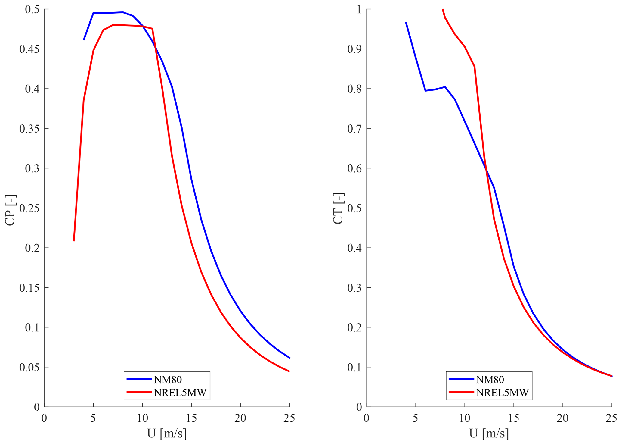
Two different three-bladed horizontal-axis wind turbines have been considered in the simulations, i.e., the NM80 and the NREL 5 MW. The NM80 turbine, see e.g., Aagaard Madsen et al. (2010), has a radius R of 40 m, a hub height z_hub of 80 m and a rated power of P₀=2.75 MW at a nominal hub height velocity of 14 m s⁻¹. The radius of the NREL 5 MW turbine is 63 m; its hub height is 90 m, and its rated power is P₀=5 MW at 11.4 m s⁻¹; see Jonkman et al. (2009). Figure 1 compares the C_P and C_T of the two turbines, which are comparable although the C_T is higher for the NREL 5 MW than for the NM80 for below rated power.

Figure 1 C_P and C_T curves for the NM80 and NREL 5 MW turbines.

3 Simulation setup

In the coordinate system used in this work, x, y and z correspond, respectively, to the streamwise, crosswise and vertical directions. The grids used for the simulations are Cartesian, and they are equidistant in the horizontal direction in all cases. The grids are usually stretched in the vertical direction from a significant distance above the wind turbines.

3.1 Atmospheric boundary layer and turbulence

All participants simulated a neutrally stratified atmospheric boundary layer (ABL). Details about the methods used to model the ABL and associated turbulence in, respectively, EllipSys3D and PALM are provided below.

3.1.1 EllipSys3D

EllipSys3D uses the prescribed boundary layer (PBL) method, in which body forces are used to impose any arbitrary vertical wind shear profile; see Mikkelsen et al. (2007) and Troldborg et al. (2014). A comparison of the PBL approach with a wall model approach was performed by Sarlak et al. (2015). This study showed that these two approaches yield very comparable vertical profiles of mean streamwise velocity, shear stress and streamwise velocity fluctuations in the rotor region when large wind farms are modeled. The present simulations use a combined parabolic and power law profile as defined in Andersen et al. (2015) and given by

$${\displaystyle }{U}_{\text{pbl}}\left(z\right)=\left\{\begin{array}{ll}{U}_{\mathrm{0}}\cdot (c_{\mathrm{2}}{z}^{\mathrm{2}}+c_{\mathrm{1}}z)& z\le {\mathrm{\Delta }}_{\text{PBL}}\\ U_{\mathrm{0}}\cdot {\left(\frac{z}{H_{\text{hub}}}\right)}^{{\mathit{\alpha }}_{\text{PBL}}}& z>{\mathrm{\Delta }}_{\text{PBL}}\end{array},\right.$$

where Δ_PBL is the height, with profile transitions from the parabolic to power law profile. H_hub is the hub height of the turbine; c₁ and c₂ are shape parameters determined to ensure a smooth transition between the parabolic and the power law expression. α_PBL is the shear exponent of the PBL.

Ambient turbulence is modeled by introducing pregenerated synthetic ambient turbulence using the Mann model; see Mann (1998). Turbulence planes are imposed at an axial position of 6 and 13R in the DTU and UU simulations, while the first simulated turbine is located at 10 and 30R from the inlet, respectively.

3.1.2 PALM

PALM uses a no-slip bottom boundary condition and the Monin–Obukhov similarity theory between the surface and the first grid level to model the atmospheric boundary layer. Random perturbations are initially imposed on the velocity fields until atmospheric turbulence has developed in a precursor simulation. The latter is performed on a smaller domain with periodic boundary conditions in the streamwise and lateral directions. The precursor results are used to initialize the full simulations with nonperiodic boundary conditions in the streamwise direction. Turbulence recycling is also applied; see Maronga et al. (2015) for details.

3.1.3 Summary of numerical methods

An overview of the numerical methods described in the previous sections are summarized in Table 1 for each of the three contributions. The performed simulations require substantial computational resources. The AL methodology typically uses 𝒪(10⁵) CPU hours for each case. The AD methodology in general requires a factor of 10–20 less due to the increased time step and decreased resolution.

Table 1 Summary of methods. The participating institutes are ForWind (FW), Uppsala University (UU) and the Technical University of Denmark (DTU).

3.2 Overview of simulations considered

A total of 18 large wind farms have been simulated and analyzed. A majority of the simulations are performed for below rated conditions at approximately 8 m s⁻¹ for a range of ambient turbulence intensities (0 %–15 %) and turbine spacings (12–20R) in the streamwise and lateral direction. Additionally, two simulations with 15 m s⁻¹ are included, which corresponds to just above rated. The simulations are summarized in Tables 2–4 for the contributions from DTU, UU and FW, respectively. The tables give the freestream wind speed at hub height U₀, ambient turbulence intensity at hub height TI, the corresponding shear exponent for a power law fit to the velocity profile in the ABL and the turbine resolution corresponding to the grid size in the vicinity of the turbines. Noticeably, the simulation differences are particularly related to the difference in modeling the atmospheric boundary layer, which gives different shear velocity profiles. The DTU simulations have previously been analyzed in terms of flow statistics and distribution in Andersen et al. (2016).

Table 2 Overview of simulations performed by DTU. The simulations include 16 turbines and 60 min of data.

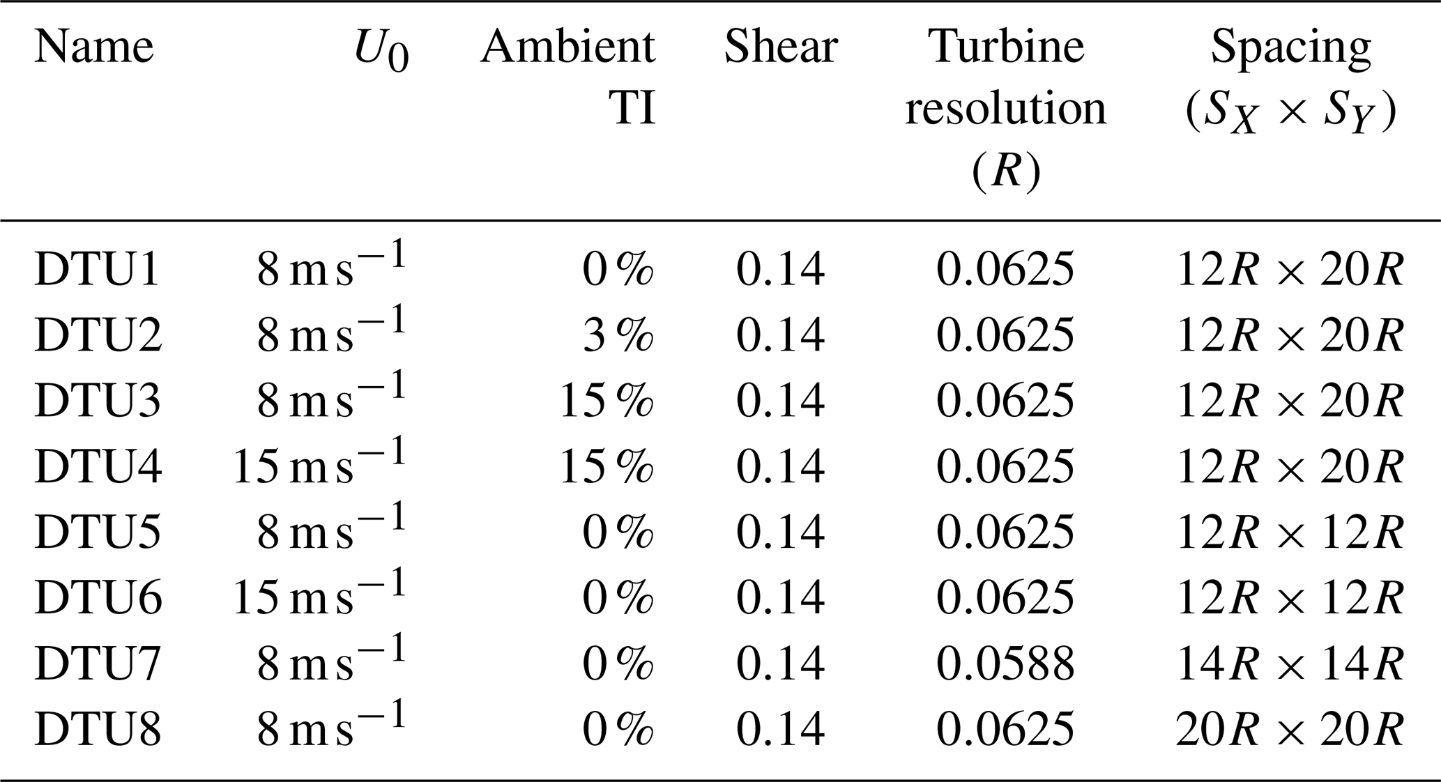
Table 3 Overview of simulations performed by UU. The simulations include 16 turbines and 30 min of data. The vertical shear profile imposed within the PBL method is determined using the same equivalent roughness as the one used in the Mann algorithm to generate turbulence (Mann, 1998).

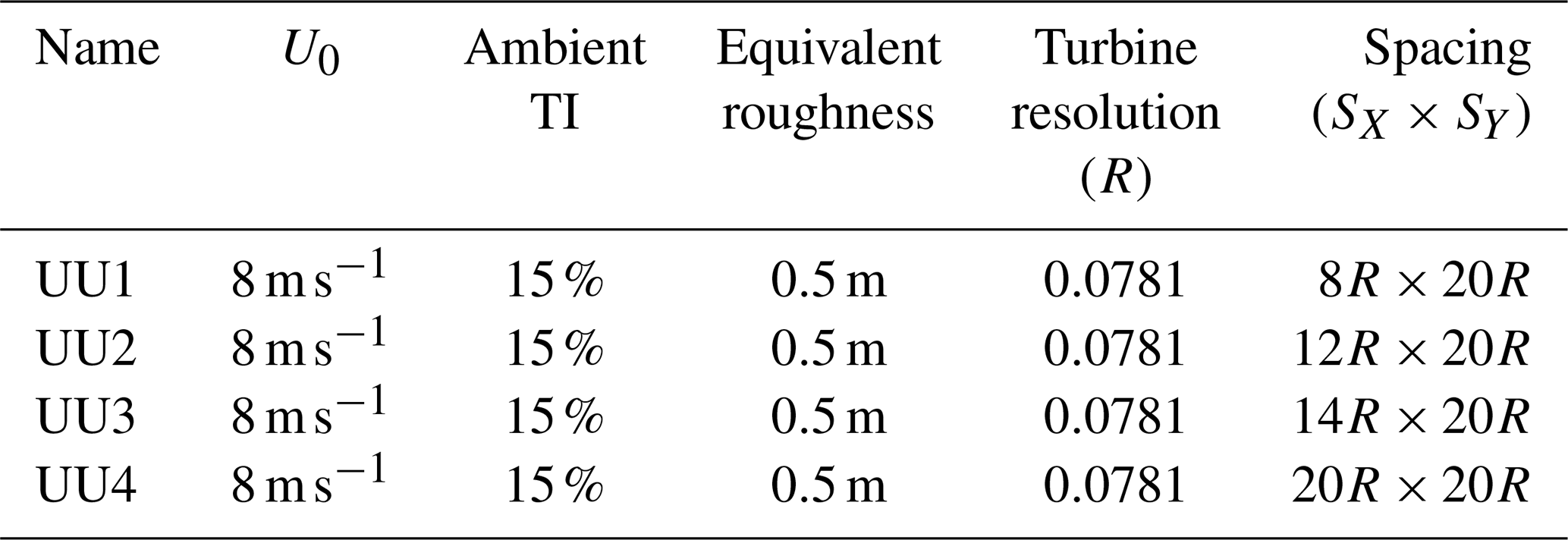
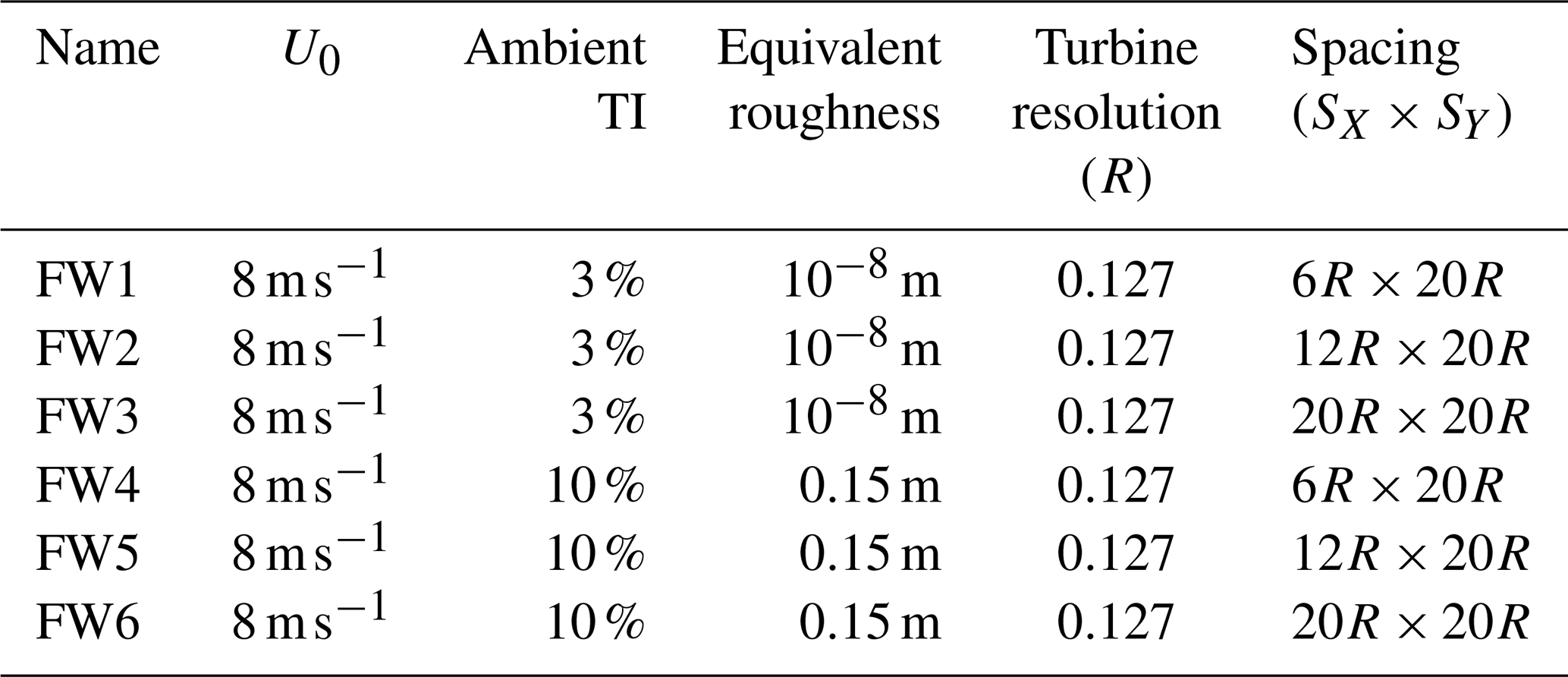
Table 4 Overview of simulations performed by FW. The simulations included two rows of 50 turbines and 60 min of data, but only data from one row of 50 turbines are used.

4 Results and discussion

The present analysis is an extension of the previous work on the inherent variability in the flow statistics in LES as presented by Andersen et al. (2015). The long-term average velocity within large wind farms is expected to converge towards a constant level deep inside the wind farm, where a balance between the extracted energy and the entrained energy is reached. However, as shown by Andersen et al. (2015) the distributions of instantaneous and even 10 min average velocities show significant variability within the same simulation. Here, the focus of the present study is on mechanical power, as opposed to the electrical power which requires estimation of the electrical losses in for instance the generator. Hence, the power production calculated as

$$P_{\text{mech}}=T\cdot \mathit{\omega },$$

where T is the torque and ω is the angular velocity.

First, the inherent variability in LES is described, before the effects of freestream turbulence intensity and of turbulence and shear combined, as well as of turbine spacing, are investigated using the different numerical setups. Finally, the large number of data are aggregated, and a more generalized analysis is performed on mechanical power production and variability within large wind farms.

4.1 Variability in LES

Simulations DTU3, UU2 and FW5 (cf. Tables 2–4) are comparable in terms of turbine spacing as well as freestream velocity and turbulence intensity at hub height, although the difference in methods yields difference in the vertical profiles of velocity and turbulence intensity. Box plots based on the 10 min average mechanical power production normalized by rated power P₀ of the first 16 turbines are given in Fig. 2. Box plots are a compact way to visualize the distribution in terms of the median and the upper and lower quartiles. The 10 min averages have been calculated for the entire time series by shifting the averaging window by 1 min to increase the number of samples, i.e., a total of 51 samples from 60 min simulation time and 21 samples from 30 min simulation time. This approach yields more samples and hence a first, albeit not statistically independent, indication of the distribution.

The results from DTU and UU are very comparable in terms of level of mechanical power production, while the FW results are approximately 40 % lower. This is consistent with the flow results presented in Andersen et al. (2015) and presumably mainly due to lower turbulence in the FW results as well as difference in shear and Coriolis effect. The figure endorses the previous findings of large variability within LES of large wind farms, although the spatial filtering effect of the turbines themselves reduces the variability in power compared to velocity. Here, the mechanical power production can vary by ±10 % or more around the median. However, there are distinct regions within the farm where the variability is higher. This is particularly evident for turbines 8–11 in the UU results. Another interesting spatial effect is seen in the results from both DTU and FW, where the median peaks at the 7th and 12th turbine. This “anomaly” was first reported by Andersen et al. (2017a) based on analysis of the same simulations, where it was shown not to be related to the atmospheric turbulence. Given the difference in numerical setup, this corroborates that the anomaly is a physical feature related to large-scale physics dependent on turbine spacing, as also discussed by Andersen et al. (2017b). These findings are furthermore corroborated by the recent experimental study by Turner V and Wosnik (2020), which identified resonance related to the turbine spacing. The simulations performed by FW included 50 turbines, so the full spatial extent of the wind farm is given in Fig. 3. The anomaly appears throughout the wind farm with distinct peaks at turbines 7, 12, 16, 23, 30, 39, 42 and 45. Furthermore, the variability clearly increases towards the end of the wind farm, where the power production ranges from 0.13 to 0.20 of rated power for the NREL 5 MW turbine.

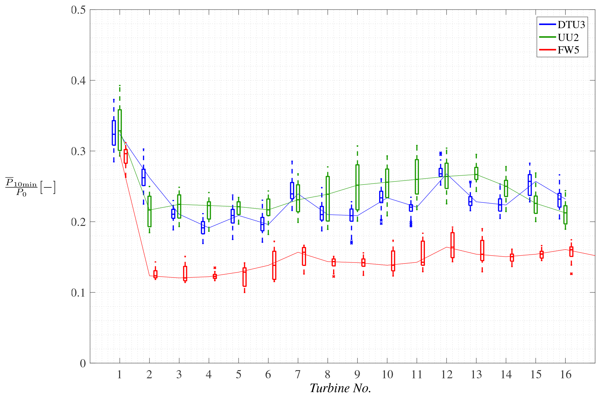
Figure 2 Box plots of the 10 min averaged mechanical power production normalized by rated power P₀ of the first 16 turbines in DTU3, UU2 and FW5. All simulations have U₀=8 m s⁻¹, S_X=12R and S_Y=20R. The turbulence intensity is TI≈15 % for DTU3 and UU2, while it is TI≈10 % for FW5. Lines connect median values of all turbines. Outliers not shown for clarity.

The variability is investigated more specifically in terms of the turbulence intensity, shear and turbulence intensity, as well as the turbine spacing, in the following.

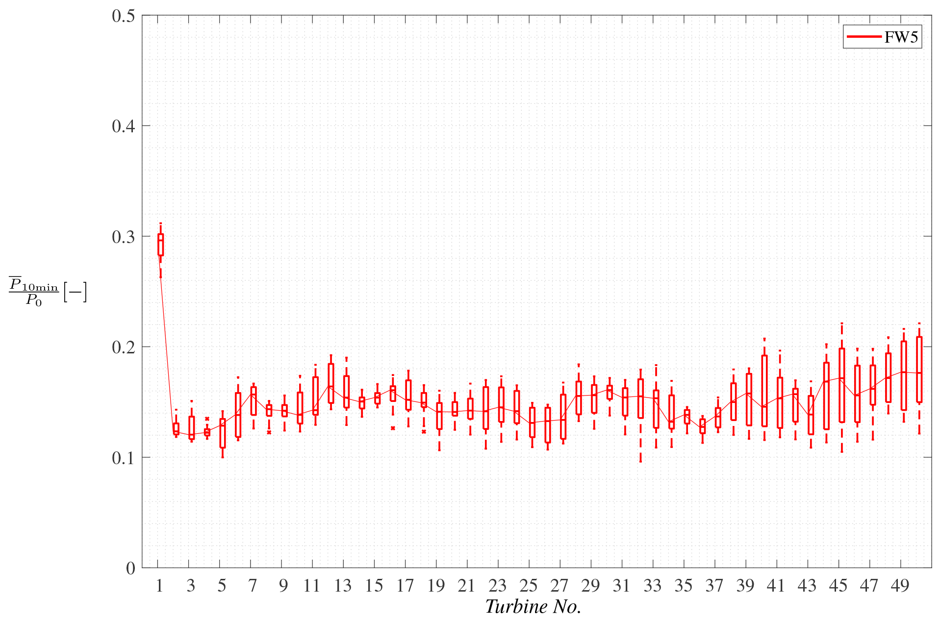
Figure 3 Box plots of all 50 turbines for FW5 with TI=10 % and $S_X\times S_Y=\mathrm{12}R\times \mathrm{20}R$. Outliers not shown for clarity.

4.1.1 Effect of turbulence intensity

The simulations from DTU and UU utilize body forces to introduce ambient turbulence into the flow. This enables direct investigation of the isolated effects of changing the ambient turbulence by changing the forcing.

Here, the distributions of instantaneous power production of the 16 turbines are compared directly in violin plots in Fig. 4 for DTU2 and DTU3, i.e., with an identical setup except an approximate freestream turbulence of 3 % and 15 %, respectively. The differences in the distributions are clear. An increase in freestream turbulence increases the mean level of power production due to increased energy entrainment. Initially, the distributions are also broader for the high-turbulence case than for the low-turbulence case, which appears Gaussian, in particular for the second turbine. The widths of the distributions become more similar further into the farm, but the difference in median level is maintained. Similar trends were reported by Andersen et al. (2016). The effect of the controller is also clearly seen as the distributions are capped around $\frac{P}{P_{\mathrm{0}}}\approx \mathrm{0.33}$, corresponding to the turbine reaching the maximum rotational speed.

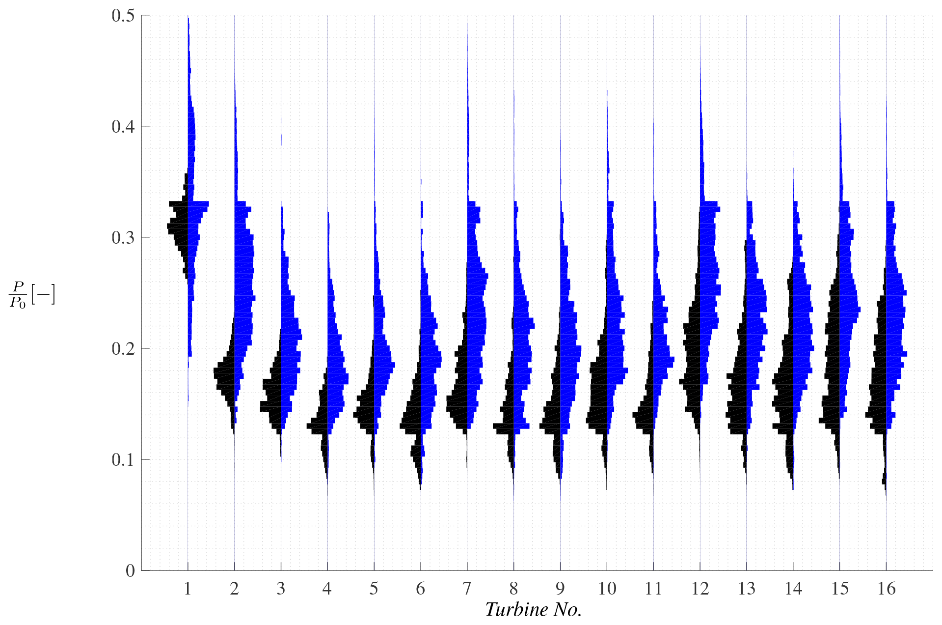
Figure 4 Violin plots comparing the influence of turbulence intensity on the instantaneous power production in DTU2 (black) with TI=3 % and DTU3 (blue) with TI=15 % for turbine spacings of $S_X\times S_Y=\mathrm{12}R\times \mathrm{20}R$.

4.1.2 Effect of shear and turbulence intensity

Turbulence intensity and shear are inherently linked in the simulations performed by FW, as a change in equivalent roughness yields different shear and turbulence profiles. Figure 5 shows violin plots of the instantaneous mechanical power production in FW2 (TI=3 %) compared to FW5 (TI=10 %) for the first 16 turbines normalized by rated power. The distribution is once again significantly broader for the high-turbulence case, and the distribution for the second turbine in the lower-turbulence case is close to Gaussian. However, the median level appears to be very similar for the following turbines (3–6) with infrequent higher tails. Further into the farm, the distributions become broader for the high-turbulence case with a slight increase in the median level. However, the increase in the median level is not as pronounced as in Fig. 4, which indicates that high shear decreases the effects of an otherwise high turbulence intensity.

Figure 5 Violin plots comparing the influence of turbulence intensity and shear on the instantaneous power production in FW2 (black) with TI=3 % and FW5 (red) with TI=10 % for turbine spacings of $S_X\times S_Y=\mathrm{12}R\times \mathrm{20}R$.

4.1.3 Effect of spacing

The initial turbulence intensity and shear discussed in the previous sections develops through wind farms, and the flow development is closely related to the turbine spacing. Figure 6 shows violin plots of the instantaneous mechanical power production in DTU5 compared to DTU7 for the first 16 turbines normalized by rated power. This allows comparing spacings of, respectively, 12R×12R and 14R×14R. This does however also relate to the turbulence intensity and shear inside the farm; see Sect. 4.1.1 and 4.1.2. The fact that these simulations consider a zero level of incoming turbulence intensity explains the small spread of power values around the mean for the first turbines in the farm. The distributions broaden as the turbulence produced by the turbines themselves dominates further into the farm. As expected, a larger spacing is associated with greater values of mean power, as it allows more time for the wake flow to mix with the outside flow in between the turbines and to recover. The power distributions associated with the greater spacing appear Gaussian for the most part, while the one related to the shorter spacing of 12R×12R is more irregular and seems to consist in two distinct parts, presumably due to how the turbine controller reacts to being in the near wake.

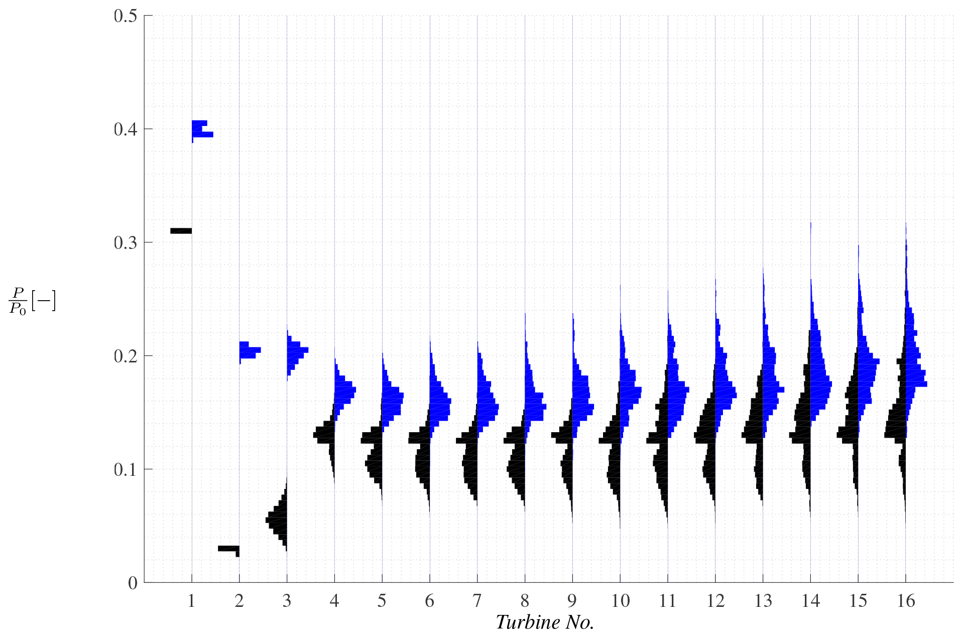
Figure 6 Violin plots comparing the influence of turbine spacing on the instantaneous power production in DTU5 (black) with $S_X\times S_Y=\mathrm{12}R\times \mathrm{12}R$ and DTU7 (blue) with $S_X\times S_Y=\mathrm{14}R\times \mathrm{14}R$, where no ambient turbulence intensity has been applied.

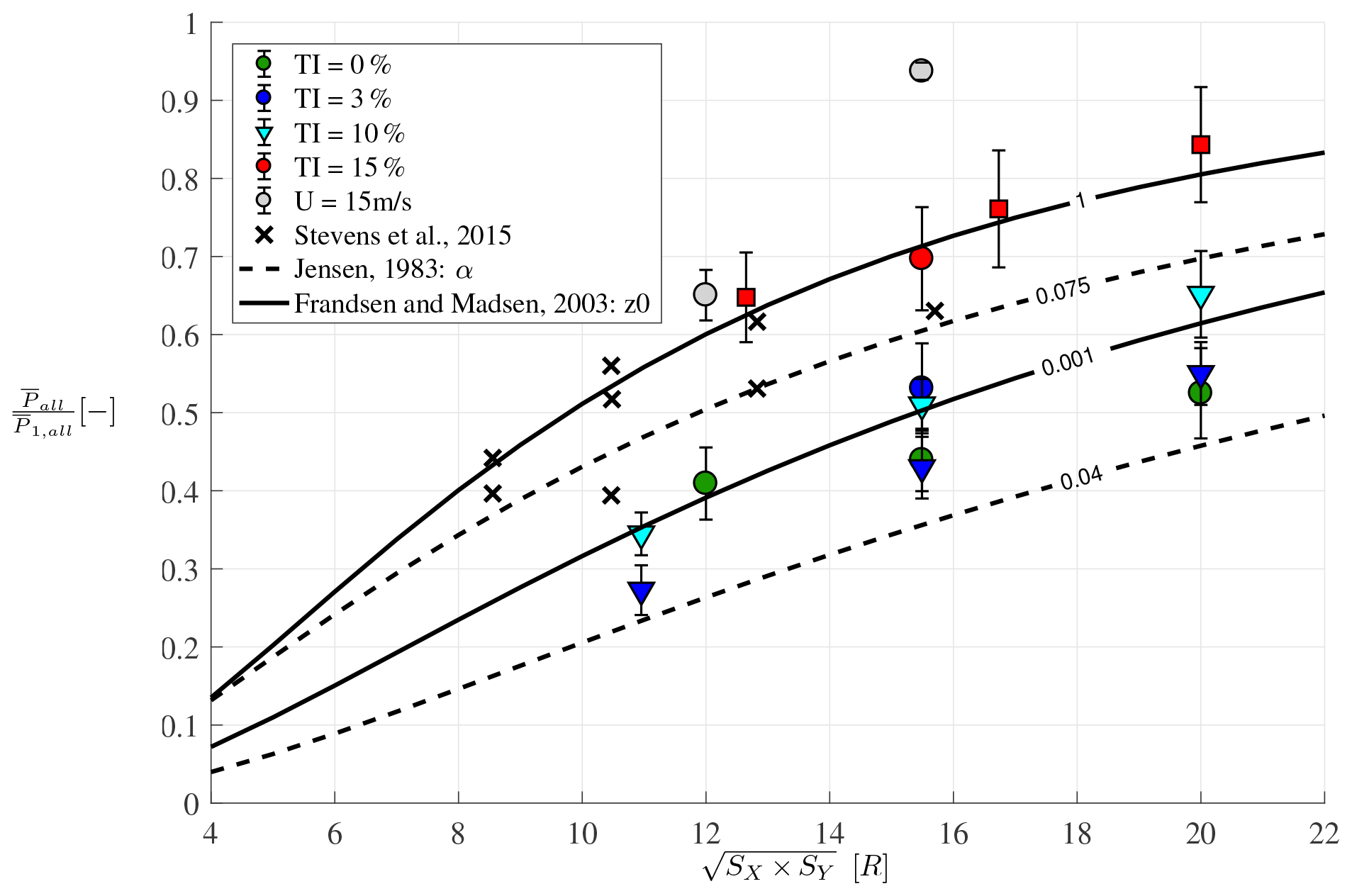
Figure 7 Mean power production of all turbines from the sixth to the end of the row for all simulations as function of representative turbine spacing. The mean power productions have been normalized by the mean power production of first wind turbine. Error bars show standard deviation of all the 10 min periods. Simulations with turbulence intensity of 0 %, 3 %, 10 % and 15 % are shown in green, blue, cyan, and red, respectively. Two simulations with $U_{\mathrm{0}}=\mathrm{15}\mathrm{m}{\mathrm{s}}^{-\mathrm{1}}$ are shown in gray, which have turbulence intensities of 0 % and 15 %. DTU results are plotted with circles, FW with triangles and UU with squares. Data from Stevens et al. (2015a), which used a constant C_T=0.75, are included for comparison. The underlying dashed contours indicate the asymptotic expression (Eq. 12) from Jensen (1983) for two different α parameters, while the full lines are contours from Frandsen and Madsen (2003) for two different z₀ values.

4.2 Aggregated data

4.2.1 Comparison to simple engineering models

The simulation data are aggregated in terms of 10 min statistics for each operating turbine. Aggregating the statistics from different simulations and numerical setups essentially assumes that all simulations are physically correct and correspond to different farms or turbines operating under different atmospheric conditions. The distributions have generally converged after the sixth turbine, despite the large variability, so the mean 10 min power production of all turbines from the sixth to the end of the row of all the 18 simulations are aggregated as representative of operating in “deep-wind-farm” conditions. The aggregated data are plotted in Fig. 7 as a function of a representative turbine spacing, $\sqrt{S_X\times S_Y}$, as suggested by Stevens et al. (2015a). The mean power production is normalized by the long-term mean power production of the first turbine to enable a direct comparison with results taken from Stevens et al. (2015a). The data are colored according to inflow turbulence intensity, and the symbols indicate if the results are from DTU, UU or FW. The standard deviations for the different 10 min periods and turbines of the current simulations have been included as error bars.

It is clear how the 18 simulations follow the same trends as the data derived from Stevens et al. (2015a) that were obtained for both aligned and staggered configurations. Stevens et al. (2015a) only present long-term averaged values without the variability. The results are generally encompassed by the results of DTU and FW. All results fall within a clear limit showing how much power can be extracted from a wind farm operating below rated wind speed depending on representative turbine spacing. An upper limit is indicated by DTU4 and DTU6 (in gray), which have a freestream velocity above rated conditions (15 m s⁻¹) but with different turbulence intensities. The power productions deep inside the farm result in below rated conditions for DTU6 due to no freestream turbulence, while the turbines in DTU4 also experience above rated velocities deep inside the farm due to the increased entrainment from the large atmospheric turbulence. Hence, it shows the transition from below rated to above rated conditions.

The effect of atmospheric turbulence is also clear, both when comparing the general trends in the plot and when comparing the DTU and FW results for different turbulent intensities. A higher atmospheric turbulence yields a higher production deep inside the farms, while low or even no atmospheric turbulence results in a lower boundary in terms of production.

Finally, the figure includes the resulting power production based on two asymptotic expressions derived by Jensen (1983) and by Frandsen (1992), respectively. The Jensen model is widely used, also by the industry, although it is less physical as it is not based on a proper momentum analysis. The model yields a velocity ratio given by

$$\begin{array}{}\text{(1)}& {{\displaystyle \frac{U_{\mathrm{\infty }}}{U_{\mathrm{0}}}}}_{\text{NOJ}}=\mathrm{1}-{\displaystyle \frac{\mathrm{2}x}{\mathrm{1}-x}},\text{ \hspace{0.17em}where\hspace{0.17em} }x={\displaystyle \frac{\mathrm{1}}{\mathrm{3}}}{\left({\displaystyle \frac{r_{\mathrm{0}}}{r_{\mathrm{0}}+\mathit{\alpha }{x}_{\mathrm{0}}}}\right)}^{\mathrm{2}}.\end{array}$$

Here, r₀ is the turbine radius and x₀ is turbine spacing, and hence, the original Jensen model only has a single input parameter, α, which governs the wake decay and expansion. The recommended values of α≈0.04 for offshore wind farms, see e.g.,  (), and α≈0.075 for onshore, see e.g., Pena Diaz et al. (2016), are also plotted for reference. The model has previously been compared to CFD simulations in Andersen et al. (2014). The power is computed from the cube of the converged velocity ratio.

The model developed by Frandsen (1992) and extended in Frandsen and Madsen (2003) is on the other hand more physical and involves more parameters, which are interlinked. Here, the expression given in Frandsen and Madsen (2003) is used, which gives the converged velocity at hub height

$$\begin{array}{}\text{(2)}& U_{h,\text{Frandsen}}={\displaystyle \frac{G}{\mathrm{1}+\ln \left(\frac{G}{f^{\prime }\cdot h}\right)\frac{\sqrt{c_t+(\mathit{\kappa }/\ln (h./z_{\mathrm{0}}){)}^{\mathrm{2}}}}{\mathit{\kappa }}}}.\end{array}$$

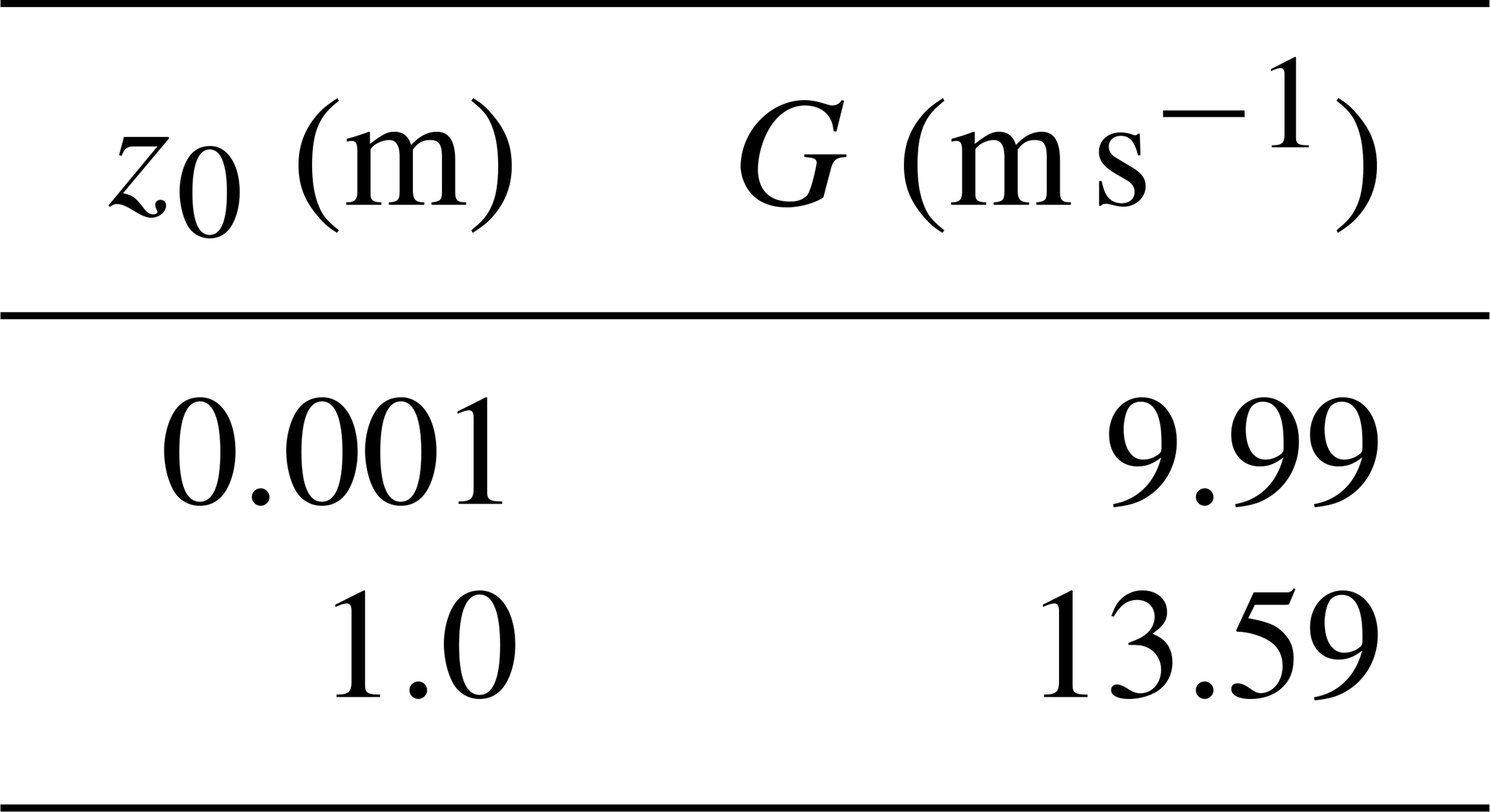
The geostrophic wind (G) and the roughness length (z₀) have an impact on the velocity at a given height. Hence, the geostrophic wind has been calibrated to give a mean wind speed of 8 m s⁻¹ at a hub height of 90 m for two realistic roughness lengths corresponding to turbulence intensities of 3 % and 15 %. A latitude of 55^∘ is assumed, and a modified parameter of $A_{*}=\mathrm{4}$ is used to compute $f^{\prime }=\mathrm{1.2}\cdot {\mathrm{10}}^{-\mathrm{4}}\cdot \exp \left(A_{*}\right)$. The geostrophic wind and roughness lengths are summarized in Table 5. The converged velocity is then found using C_T=0.8 for various distances. The mean power production ratio is then computed using the cube of the converged velocity ratio and assuming constant C_T.

Table 5 Calibrated geostrophic wind speeds (G) and corresponding roughness length (z₀), which yield a wind speed of 8 m s⁻¹ at a hub height of 90 m.

Both models capture the general trends very well, although the Jensen model underestimates the actual power production for the recommended values. The Frandsen model performs very well and captures both the high and low turbulence intensity levels as well as the gradual change for the lower turbine spacings where the data by Stevens et al. (2015a) are located. The simpler models give a good first estimate of the converged mean power production, but the simpler models do not capture the inherent variability in the power production, as the models are merely steady state. The continued importance of developing and testing such analytical models to provide accurate estimates of both mean velocity and variability was discussed in detail by Meneveau (2019).

4.2.2 Response surfaces

The total number of aggregated data in Fig. 7 comprises 12 016 different, albeit overlapping, 10 min realizations, which include the variability, both within a given 10 min realization and between different 10 min realizations as shown previously.

The power per ground area, or power density, compared to the standard deviation of power normalized by the mean power for different relative spacings is shown in Fig. 8, where each dot is a 10 min realization. The green dots show results with low atmospheric turbulence (TI=0 %–3 %), while the red dots show results for high turbulence (TI=10 %–15 %). The bin-averaged data are shown in black with the standard error plotted as error bars. The standard error is here defined as

$$\begin{array}{}\text{(3)}& {\mathit{ϵ}}_{\text{std}}={\displaystyle \frac{\mathit{\sigma }\left(\frac{{\stackrel{\mathrm{‾}}{P}}_{\mathrm{10}\text{min}}}{S_X\times S_Y}\right)}{\sqrt{N}}},\end{array}$$

i.e., the standard deviation of the power density within a given bin normalized by the square root of the number of observations.

The data show significant spread in both power per area and standard deviation of the power although all simulation results generally cluster together. The binned values are generally very consistent except at low standard deviations, in particular Fig. 8a and e, where the binned values jump. The standard error is usually small as the limited number of samples are located in small clusters, except in Fig. 8a, which shows large standard deviations of the binned data. Furthermore, it appears that the power production per ground area is not very influenced by the standard deviation normalized by mean power. The high-atmospheric-turbulence realizations (in red) generally result in a larger power density, as expected. Interestingly, the low-atmospheric-turbulence realizations yield larger standard deviations of the power within the realization; see Fig. 8a, e and g.

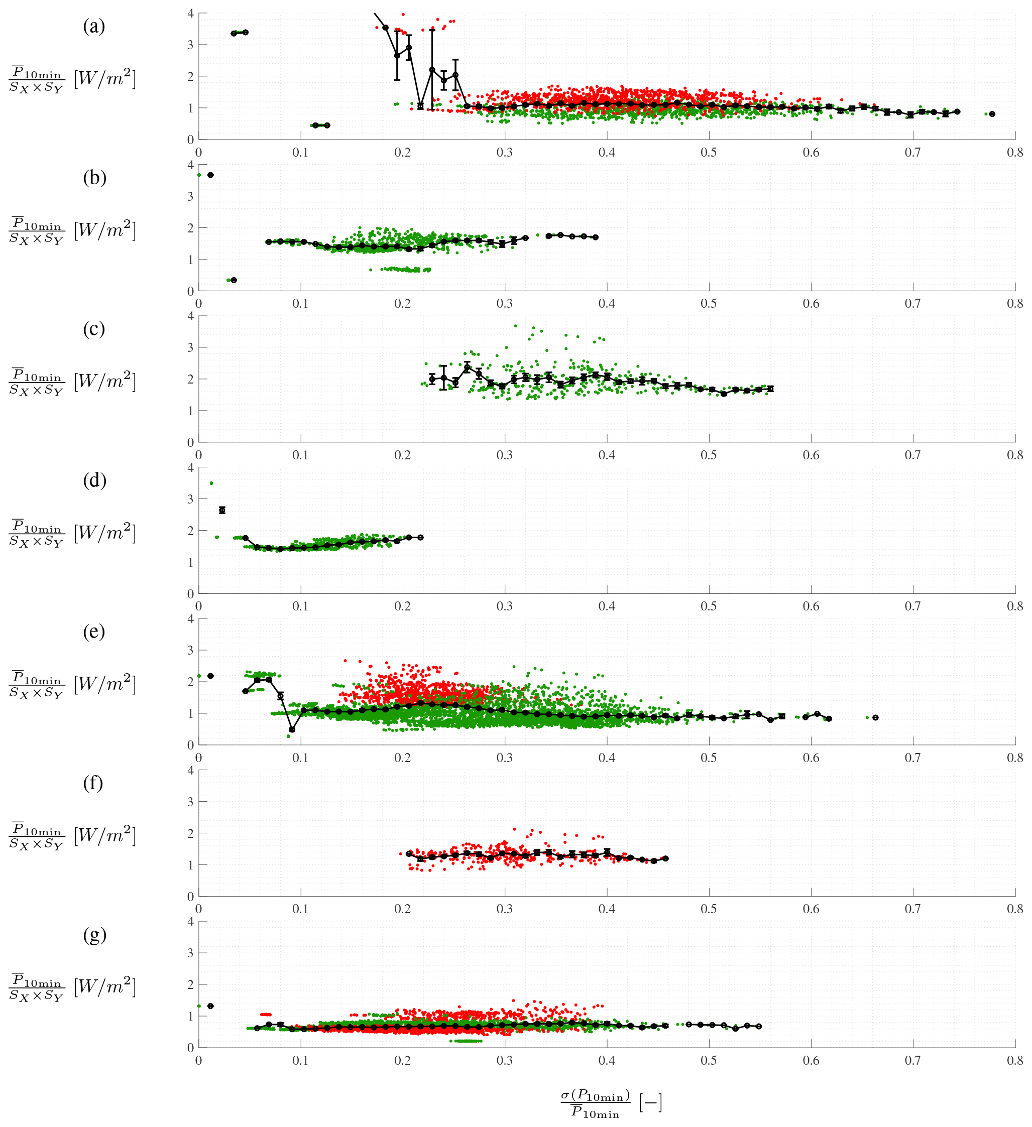
Figure 8 Power per ground area plotted against standard deviation of power normalized by mean power for (a) $\sqrt{(S_X\times S_Y)}=\mathrm{10.95}R$, (b) $\sqrt{(S_X\times S_Y)}=\mathrm{12.00}R$, (c) $\sqrt{(S_X\times S_Y)}=\mathrm{12.65}R$, (d) $\sqrt{(S_X\times S_Y)}=\mathrm{14.00}R$, (e) $\sqrt{(S_X\times S_Y)}=\mathrm{15.49}R$, (f) $\sqrt{(S_X\times S_Y)}=\mathrm{16.73}R$ and (g) $\sqrt{(S_X\times S_Y)}=\mathrm{20.00}R$. The green dots indicate results with low atmospheric turbulence (TI=0–3 %), while the red dots indicate results for high turbulence (TI=10–15 %). The black dots show bin-averaged values including the standard error plotted as error bars.

Figure 9 Contours based on multiple linear regression fit of bin-averaged power production per area to the standard deviation of power production normalized by mean power production and relative turbine spacing. Points mark the binned data, where blue and red shades indicates whether the fit underestimates or overestimates, respectively, the binned averaged values.

A multiple linear regression is applied to the full set of bin-averaged data with a freestream velocity of 8 m s⁻¹ from Fig. 8, i.e., aggregating all data with comparable C_T. The regression is fitted in a least-squares sense using the MATLAB function “regress”¹. The regression fits the bin-averaged power production per area to the normalized standard deviation of the power production and the relative turbine spacing. The fit is performed to second order, i.e., for combinations of ${\mathbf{S}}^{*}=\sqrt{{\mathit{S}}_X\times {\mathit{S}}_Y}$ and ${\mathit{\sigma }}^{\mathbf{*}}=\frac{{\stackrel{\mathrm{‾}}{P}}_{\mathrm{10}\min }}{{\mathit{S}}_X\times {\mathit{S}}_Y}$ of the following matrix:

$$\begin{array}{ll}\text{(4)}& {\displaystyle }\stackrel{\mathrm{̃}}{A}& {\displaystyle }=\underset{\mathrm{¯}}{b}\left(\mathrm{1}\right)+\underset{\mathrm{¯}}{b}\left(\mathrm{2}\right)\cdot {\mathbf{S}}^{*}+\underset{\mathrm{¯}}{b}\left(\mathrm{3}\right)\cdot {\mathit{\sigma }}^{\mathbf{*}}+\underset{\mathrm{¯}}{b}\left(\mathrm{4}\right)\cdot {\mathbf{S}}^{*}\cdot {\mathit{\sigma }}^{\mathbf{*}}{\displaystyle }& {\displaystyle }+\underset{\mathrm{¯}}{b}\left(\mathrm{5}\right)\cdot {{\mathbf{S}}^{*}}^{\mathrm{2}}+\underset{\mathrm{¯}}{b}\left(\mathrm{6}\right)\cdot {{\mathit{\sigma }}^{\mathbf{*}}}^{\mathrm{2}}.\end{array}$$

The fit gives the coefficients $\underset{\mathrm{¯}}{b}$, and the combined set yields a response surface of the fit.

Figure 9 shows a contour plot of the response surface. The power density found here for a freestream velocity of 8 m s⁻¹ is in the range of 0.5–2.0 W m⁻², which is comparable to the general range of 1–11 W m⁻² reported by Denholm et al. (2009). The power density clearly decreases when the relative turbine spacing increases, as expected, because although the power production increases for larger spacing, the area increases faster and hence dominates the ratio. However, it is also clear how the power density varies with the standard deviation of the power production, i.e., how much power the turbines are able to exploit and extract from the turbulent fluctuations. For large spacing, the power density is not influenced significantly by the standard deviation of the power production, cf. Fig. 8g. For smaller spacing, there is an increased power density for small standard deviations in the power production, albeit related to the aforementioned small clusters of increased power density for small spacing, particularly seen in Fig. 8a.

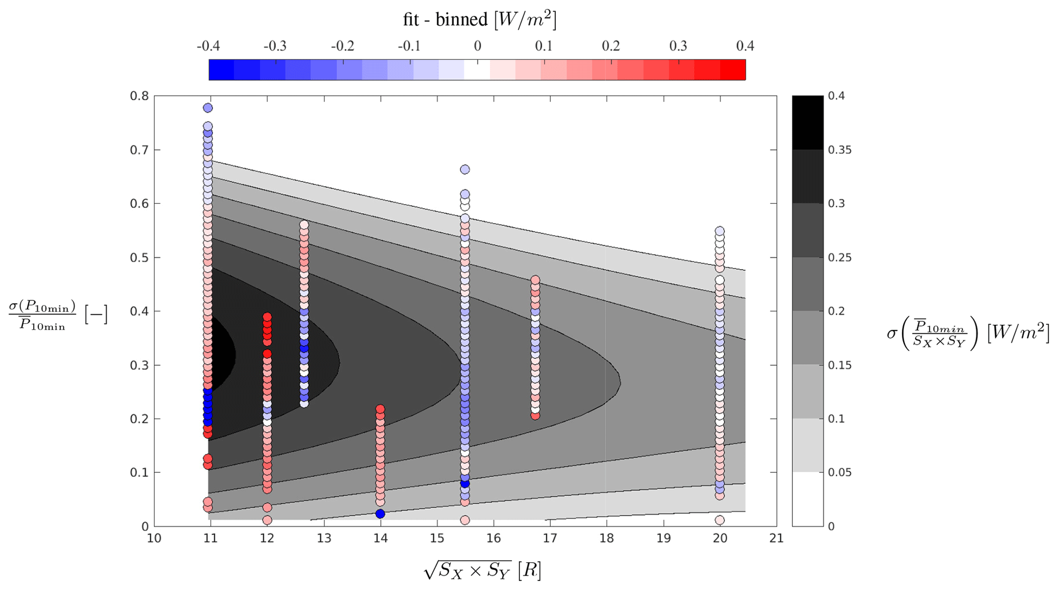
Figure 10 Contours based on multiple linear regression fit of standard deviation of the bin-averaged power production per area to the standard deviation of power production normalized by mean power production and relative turbine spacing. Points mark the binned data, where blue and red shades indicate whether the fit underestimates or overestimates, respectively, the binned averaged values.

Figure 9 also includes circles indicating the binned data used for the fit. The circles are colored according to the difference between the fit and the binned data. The difference is generally (87 % of the binned data points) less than ±0.5 W m⁻² and alternating between a positive and negative difference for different relative spacings. The fit is particularly good for larger spacings, but it struggles for smaller spacings with large outliers. The sensitivity of the fit is examined by performing a 10-fold cross-validation. The mean squared error (MSE) is estimated between the fitted response surface and the actual input data. The resulting MSE is 0.0732±0.0011 indicating that the fit is consistent across the data but that an improved response surface could be created. However, this would presumably also require a larger number of data.

As shown previously, the simple engineering model by Frandsen (2007) is capable of capturing the average trends, similar to the response surface. However, the inherent variability in LES is important for farm performance and for improving risk assessment during the design phase. Hence, a similar response surface can be fitted to the standard deviation and the standard error in the bin-averaged values in Fig. 8. The corresponding response surfaces are shown in Figs. 10 and 11, which can be interpreted as the variability and the uncertainty associated with the response surface of mean power density.

The variability around the mean is up to 0.4 W m⁻² for small relative spacings, which is comparable to the difference in the fit and bin-averaged data as shown before. The variability is higher for shorter spacings, where the number of outliers affects the fit. The outliers can be related to the significant nonlinearities in the near wake before the wake breaks down into small-scale turbulence; see Sørensen et al. (2015). The 10-fold cross-validation on the variability yields $\text{MSE}=\mathrm{0.0276}\pm \mathrm{0.0014}$, which indicates a significant uncertainty in the fit but again very small variation within the given dataset.

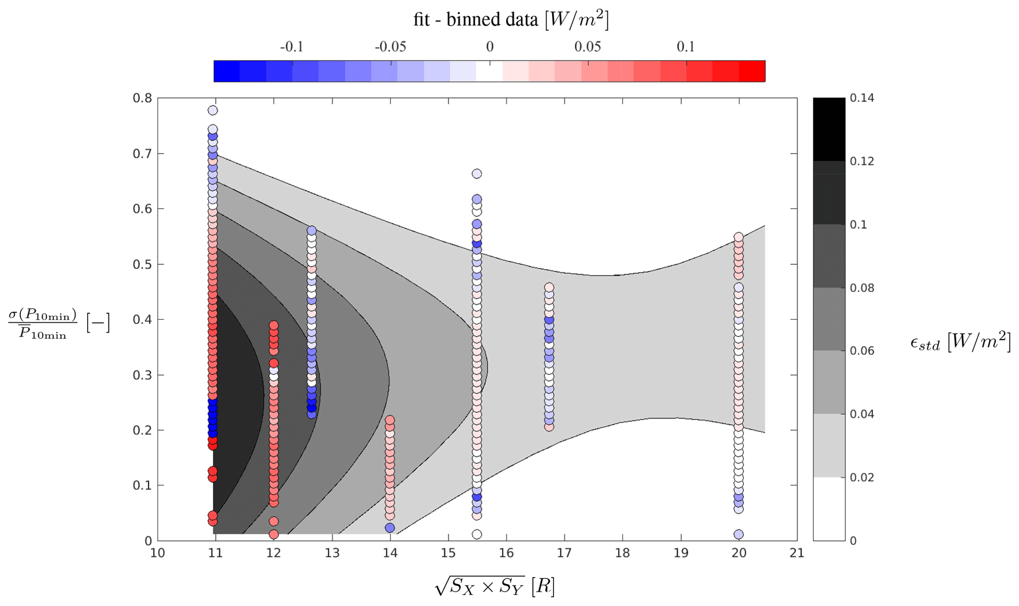
Figure 11 Contours based on multiple linear regression fit of the standard error in the bin-averaged power production per area to the standard deviation of power production normalized by mean power production and relative turbine spacing. Points mark the binned data, where blue and red shades indicate whether the fit underestimates or overestimates, respectively, the binned averaged values.

The increased variability for smaller spacing also comes with an increased uncertainty as shown in Fig. 11. The standard error decreases for increasing spacing, where the fit is very good, while the discrepancy is larger for the very short distance. The fit tends to overestimate the standard error for the shortest spacings. Again, a 10-fold cross-validation is performed on the response surface for the uncertainty, which gives $\text{MSE}=\mathrm{0.0085}\pm \mathrm{0.0015}$. This is, again, a very small variation within the given dataset but indicates that the chosen response surface could be improved.

The response surfaces are only fitted to second order, because the aim here is merely to provide general insights into the global trends and hence to avoid overfitting. It should be strongly emphasized that this is a rather crude approach. However, the response surfaces yield a first attempt at constructing global response surfaces of the power density including the inherent variability based on significant numbers of LES data for a wide range of wind farm layouts operating at 8 m s⁻¹, which show physical trends.

Figure 12 shows a heatmap of how the 10 min realizations are distributed for the standard deviation of power production within each 10 min period normalized by the corresponding power production versus the relative turbine spacing. Clearly, a majority of 10 min realizations are in the range of $\frac{\mathit{\sigma }\left(P_{\mathrm{10}\min }\right)}{{\stackrel{\mathrm{‾}}{P}}_{\mathrm{10}\min }}=[\mathrm{0.1}$, 0.5] for $\sqrt{S_X\times S_Y}=\mathrm{15.49}R$ and $\sqrt{S_X\times S_Y}=\mathrm{20}R$. The presented response surfaces are directly dependent on the data availability and hence most representative in this range, and care should therefore be taken in the ranges with few realizations. However, Fig. 12 can be used to guide which scenarios should be computed next essentially to fill the gaps. As such, additional LES computations should be focused around $\sqrt{S_X\times S_Y}=\mathrm{16}R$, 18–19R, where there is no data, and $\sqrt{S_X\times S_Y}<\mathrm{14}R$, where the uncertainty is large. The response surfaces can therefore continuously be improved by adding more data, and a more sophisticated response surface or surrogate can be constructed once the entire parameter space is full.

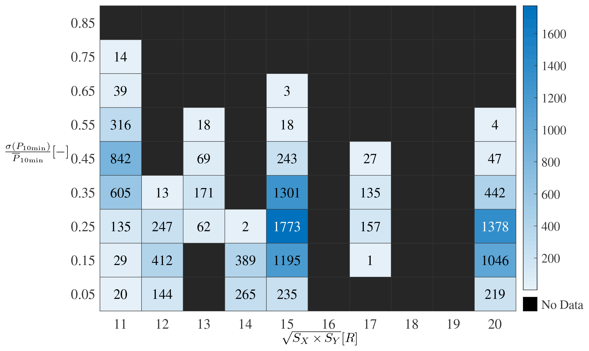
Figure 12 Heatmap showing number of 10 min realizations for different bins of relative spacing and standard deviation of power production based on a total of 12 016 realizations. Values on axes show center value.

The response surfaces could also be made dependent on more parameters by adding more LES data. Currently, the turbine spacings in the lateral and streamwise direction have been collapsed to a single dimension, but the dependency could be unfolded. Similarly, the dependency on a number of additional parameters could be investigated, for instance,

• free wind speed,

• turbulence level,

• atmospheric stability,

• shear,

• turbine size.

However, this would obviously require substantial amounts of computing resources.

One way to circumvent the large computational costs would be to utilize supervisory control and data acquisition (SCADA) data in combination with the LES. Similar response surfaces could be constructed based on SCADA data from operating wind farms, which would enable a more global verification of LES and the actuator disc and line methods on a wind farm scale. Such a verification would be valuable as direct comparison of time series of specific events between LES and actual wind farms is extremely difficult, if not impossible, to achieve given the complexity and amount of information required on the atmospheric conditions to enable such a comparison.

A successful verification would facilitate the direct integration of LES data and SCADA data to construct more certain response surfaces covering a larger range of scenarios and parameters. It could act as a lodestar and inform researchers about in which regions of turbine spacing and turbulence intensity to perform the expensive LES in order to fill the gaps and explain physical trends not captured by the simpler models.

Finally, the response surface could be extended to include e.g., fatigue loads for turbines operating in wind farms. Such a surrogate model for fatigue loads on a single wind turbine was developed by Dimitrov et al. (2018), who compared the accuracy and performance of six different methods.

5 Conclusions

This work aimed at providing a general overview of the global trends in power performance for large wind farms, with a focus on variability. This was done through the analysis of large eddy simulation (LES) performed on large wind farms from the three institutions behind this work. LES results of large wind farms obtained from other researchers as well as simulations performed using simpler engineering models were also included to provide a more complete envelope for the results.

As LES requires large amounts of computational resource, emphasis was placed on extracting as much information as possible from the existing set of simulations performed using different setups and incoming flow conditions. As such, emphasis is not put on comparing the simulations to each other but rather on using as many results as possible to cover a wide range of possible scenarios that can provide a global picture of the power characteristics within large wind farms.

Parametric studies were first performed to inform about the effect of atmospheric conditions as well as turbine spacing on production and its variability. An increase in atmospheric turbulence intensity, by increasing energy entrainment, was shown to raise the mean level of power production. It was also associated with wider distributions of the production values. A larger spacing between the turbines was also associated with greater levels of production, as expected.

The analysis was extended further by aggregating the large number of LES runs performed under various conditions. This was carried out in terms of 10 min statistics for each turbine operating in deep-farm conditions. LES works from other researchers as well as simulations performed with simpler engineering models were also included in a first step when looking at the power produced deep inside the farm as a function of a representative spacing. All results were shown to fall within a clear limit showing how much power can be extracted from a wind farm operating below rated wind speed, as a function of representative turbine spacing. Whereas higher turbulence levels lead to larger production levels deep inside the farms, cases without incoming turbulence were shown to provide lower power production. While LES provides more information in terms of variability, simple engineering models were shown to produce a reasonable envelope for the results obtained using the high-fidelity methods.

As a second step, response surfaces encompassing the total number of aggregated LES data, i.e., 12 016 different albeit overlapping 10 min realizations, were created. They revealed information regarding various aspects of the power production within large wind farms, including the amount of power the turbines are able to extract from the turbulent fluctuations, as well as the variability and uncertainty associated with the mean power densities.

The work presented in this paper serves to provide valuable information regarding power and its variability deep inside large wind farms. Nonetheless, the response surfaces presented here would gain from being complemented with more LES results to provide an even more complete picture. This could be done by considering further turbine spacings to fill existing gaps. The dependency of response surfaces on more parameters could also be investigated, including individually considered spanwise and streamwise spacings and the freestream velocity as well as the atmospheric stability. As LES is known to be very computationally demanding, SCADA data could also be used to provide more complete response surfaces. Future work could also go one step further by investigating the behavior of turbine loads in similar terms to what was performed here regarding power production.