the Creative Commons Attribution 4.0 License.
the Creative Commons Attribution 4.0 License.
 | 29 Jan 2020
Reliability-based design optimization of offshore wind turbine support structures using analytical sensitivities and factorized uncertainty modeling
Michael Muskulus
The need for cost-effective support structure designs for offshore wind turbines has led to continued interest in the development of design optimization methods. So far, almost no studies have considered the effect of uncertainty, and hence probabilistic constraints, on the support structure design optimization problem. In this work, we present a general methodology that implements recent developments in gradient-based design optimization, in particular the use of analytical gradients, within the context of reliability-based design optimization methods. Gradient-based optimization is typically more efficient and has more well-defined convergence properties than gradient-free methods, making this the preferred paradigm for reliability-based optimization where possible. By an assumed factorization of the uncertain response into a design-independent, probabilistic part and a design-dependent but completely deterministic part, it is possible to computationally decouple the reliability analysis from the design optimization. Furthermore, this decoupling makes no further assumption about the functional nature of the stochastic response, meaning that high-fidelity surrogate modeling through Gaussian process regression of the probabilistic part can be performed while using analytical gradient-based methods for the design optimization. We apply this methodology to several different cases based around a uniform cantilever beam and the OC3 Monopile and different loading and constraint scenarios. The results demonstrate the viability of the approach in terms of obtaining reliable, optimal support structure designs and furthermore show that in practice only a limited amount of additional computational effort is required compared to deterministic design optimization. While there are some limitations in the applied cases, and some further refinement might be necessary for applications to high-fidelity design scenarios, the demonstrated capabilities of the proposed methodology show that efficient reliability-based optimization for offshore wind turbine support structures is feasible.
- Article
(3745 KB) - Full-text XML
-
Supplement
(312 KB) - BibTeX
- EndNote


Offshore wind energy is becoming an increasingly competitive alternative to the traditional land-based wind farms. However, there remains a level of additional cost which, together with some practical challenges, ensures that offshore wind is still a secondary consideration in many markets. Hence, the reduction of this cost is a primary objective in current research and development. Cost reduction is generally a multidisciplinary issue, including turbine components like rotor blades and the drivetrain, wind farm layout, the electrical grid and the design of the support structure (including the tower). Methods to derive cost-effective, optimal support structure designs – balancing minimal use of materials (and potentially other cost-driving design aspects) with the ability to safely withstand the loads required by design standards – have been an active area of research for many years. However, very few studies have taken into account the probabilistic, fundamentally uncertain aspects of the design process. This includes, for example, uncertainties in the environment and the modeling of the environment, affecting the loads experienced by the structure, as well as uncertainties about the details of the design itself, affecting the response to the applied loads. Taking such uncertainties into account generally requires the use of probabilistic mathematical methods that severely complicate the design optimization problem that needs to be solved, both formally and numerically. Hence, deterministic safety factors tend to be used. This is also true even for single design assessments. The present study aims to address these issues by proposing a methodology that allows the use of both state-of-the-art optimization methods recently developed for support structure design and probabilistic assessments of the structural response to both fatigue and extreme loads.
Design optimization of structures subject to probabilistic problem variables and parameters, sometimes called optimization under uncertainty, is in general a large field of research at the intersection of two larger fields, optimization and probabilistic design. One main distinction is between robust design optimization (RBO) (Ben-Tal et al., 2009; Zang et al., 2005) and reliability-based design optimization (RBDO) (Choi et al., 2007; Valdebenito and Schuëller, 2010a). The main difference between the two methods is that in RBDO the design is optimized normally but under specific probabilistic limits on structural performance (probability of failure), whereas in RBO the basic idea is to minimize the variance of a probabilistic objective function in order that the obtained (mean) solution is robust with respect to the uncertainties. We will generally restrict our discussion to RBDO and reliability methods but refer to studies on RBO and robust methods where necessary or appropriate. Furthermore, given the extensive research on more general applications of reliability analysis, optimization and RBDO (or optimization under uncertainty more generally), we will focus on previous studies concerning wind turbines. For a more expansive overview of structural reliability and RBDO applied to wind turbines than the one following below, the interested reader is referred to Jiang et al. (2017), Leimeister and Kolios (2018), Hübler (2019) and Hu (2018).
A substantial amount of the literature for both structural reliability analyses and RBDO of offshore wind turbines (OWTs) has focused on aspects other than support structure design. Areas such as blade design (Ronold et al., 1999; Toft and Sørensen, 2011; Dimitrov, 2013; Hu et al., 2016; Caboni et al., 2018), foundation design (Yoon et al., 2014; Carswell et al., 2015; Depina et al., 2016, 2017; Haj et al., 2019; Velarde et al., 2019), component design (Kostandyan and Sørensen, 2011; Rafsanjani et al., 2017; Lee et al., 2014; Li et al., 2017), system/wind farm aspects (Sørensen et al., 2008), inspection and maintenance planning, and probabilistic tuning/optimization of safety factors (Sørensen and Tarp-Johansen, 2005; Márquez-Domínguez and Sørensen, 2012; Veldkamp, 2008) have all been studied. As for support structure design specifically, though most structural analyses of OWTs remain deterministic, there has been a number of studies incorporating reliability-based (or otherwise probabilistic) approaches. For the most part, the reliability-based analyses can be divided into two categories. Firstly, there are studies using simplified probabilistic models where the uncertainty in the response is assumed to be a product of the underlying stochastic variables and the deterministic response variable (e.g., Thöns et al., 2010; Sørensen and Toft, 2010; Wandji et al., 2016; Yeter et al., 2016, as well as several of the previously cited studies). Note that the basis for this kind of factorization can be justified partially or entirely depending on both the type of response variable and the type of stochastic variable. For example, in the case of Yeter et al. (2016), the stochastic variables are mostly either modeling or simulation errors, or directly originating within the analytical expressions for the response variable. Hence, the level of approximation involved in this kind of probabilistic modeling varies. While not strictly in the same category, studies where the fatigue calculation is based on crack propagation models and an assumption that the stress cycles follow a Weibull distribution, allowing exact limit state expressions to be derived, should be mentioned (e.g., Dong et al., 2012). Generally, these simplifications are done in order to be able to solve the reliability problem using first-/second-order reliability methods (FORMs/SORMs) in a computationally feasible way. In the second category of studies, the response itself is simplified, while generally no particular assumptions about the stochastic nature of the response are made. This has been done through static response modeling (e.g., Wei et al., 2014; Kim and Lee, 2015), but usually the response is replaced by surrogate models of some kind (e.g., Kolios, 2010; Teixeira et al., 2017; Morató et al., 2019). The use of surrogate models is often done in order to be able to solve the reliability problem by sampling methods, generally requiring a large number of response evaluations, but surrogate models also make FORM/SORM more computationally practical. Note that this division of reliability methodology is not strict – Thöns et al. (2010) also makes use of surrogate modeling, for example – nor does it cover all approaches, but it is useful as an indicator for one of the fundamental struggles that all the aforementioned studies have reckoned with: the fidelity of the probabilistic modeling vs. the fidelity of the underlying structural analysis.
Only a limited number of studies applying RBDO to OWT support structure design have been made. In a series of studies, Yang and collaborators investigated optimization of a tripod support structure with probabilistic constraints. In Yang et al. (2015), RBDO was performed, and in Yang and Zhu (2015), RBO was performed. In both cases, a Gaussian process (kriging) surrogate model was used for the response and Monte Carlo sampling was used for the reliability calculation. In Yang et al. (2018), RBDO was once again performed with a Gaussian process surrogate model, but in this case the reliability calculation was done using a fractional moment method in order to reduce the number of system evaluations required. All three studies used the heuristic optimization method called the multi-island genetic algorithm, and the reliability calculations were done for each step in the optimization loop, creating a nested two-loop structure. As one might expect from a heuristic method, the number of iterations required to solve even the deterministic optimization problem (around 300 iterations) is rather large given the small number of design variables used, and this is much more pronounced in the case of the stochastic optimization (around 3000 iterations). This means that the method is rather computationally inefficient, especially considering the number of system evaluations required by the reliability calculation and the genetic algorithm at each iteration. However, due to the use of the surrogate model, this practical issue is overcome, if still apparent. Though not an application to OWTs, it is also worth mentioning the study of RBDO applied to offshore monopod towers in Karadeniz et al. (2010b) and applied to jacket structures in Karadeniz et al. (2010a). Here, the limit state functions are formulated analytically, and a nested two-loop approach using gradient-based optimization (in this case sequential quadratic programming, SQP) and FORM is used.
The previous work on RBDO for OWTs (for both support structures and otherwise) demonstrates that these methods can obtain optimal designs that are both more robust/safe with respect to uncertainties than designs optimized under deterministic criteria and more tailored to specific design conditions than deterministic designs using safety factors. However, so far (and this is particularly true for support structure designs), no studies have taken advantage of recent advances in deterministic structural optimization methodology. Optimization methods in general can be divided into gradient-based and gradient-free (often heuristic) methods. Both approaches have been applied to support structure design and other wind turbine components (both on- and offshore). With some exceptions (e.g., Negm and Maalawi, 2000 using an interior penalty method), gradient-free methods were the most common among earlier studies. Examples include Yoshida (2006) using a genetic algorithm, Uys et al. (2007) with a Rosenbrock search and Zwick et al. (2012) with a local scaling of sectional members. The advantages of these approaches are that no gradient information is needed for the optimization, which simplifies the calculations that need to be performed for each iteration and avoids the reliance on finite difference methods, which can be unstable in some implementations. On the other hand, these methods, at least when done at a similar level of detail, generally converge much slower than gradient-based alternatives, where the search for optimal designs can be more specifically guided by the information provided by the gradients. With this disadvantage of gradient-free methods in mind, and seeking to avoid the issues related to finite difference methods, some recent studies have demonstrated the viability and, in most cases, advantages of analytical sensitivities in gradient-based formulations. This has been shown for static (Sandal et al., 2018), quasi-static (Oest et al., 2017) and dynamic (Chew et al., 2016) loading conditions (see also Oest et al., 2018 for a comparison of these three approaches and a more thorough review of support structure optimization). In general, these approaches make the design optimization problem more efficient and stable, though, because of the added conceptual complications, these methods have yet to be applied in studies considering a more realistic and comprehensive set of loading conditions. A study founded on gradient-based optimization that does consider a more comprehensive set of loading conditions but does not utilize analytical sensitivities was performed by Häfele et al. (2019). They used a Gaussian process surrogate model to simplify the response, thus making the analysis computationally feasible. This study also used a more complicated and (arguably) more realistic objective function, modeling the cost of the support structure in a more detailed way than the strictly steel mass-/volume-based approaches that are otherwise commonly used. However, it was seen that, at least with the particular cost formulations used, the solution was more or less the same as when a simpler mass-based objective function was used. Another recent study regarding deterministic support structure optimization was done in Couceiro et al. (2019). Like the previous study, completely analytical sensitivities were not used. The plausibility of more comprehensive code checks for design optimization under dynamic loading was in this case demonstrated by a simplified fatigue extrapolation procedure and an aggregation of time-dependent stress constraints (for ultimate limit state analysis) into a single constraint per stress time series. All these studies have been focused on bottom-fixed structures (jackets in particular, though the methodologies are easily transferable to monopiles) and it is unclear what level of adaptation is necessary to extend these formulations to floating structures.
As seen in several of the cited studies above, the use of surrogate modeling to simplify the response analysis has become more common recently. For optimization and reliability analysis, and all the more so for RBDO, this is a natural way to make the problems more computationally tractable when faced with having to perform a large number of time-consuming simulations. However, surrogate modeling is increasingly also proposed for basic structural analysis due to the large number of environmental states that need to be checked for certification according to design standards (e.g., International Electrotechnical Commission, 2009). For example, Toft et al. (2016a) used a response surface based on Taylor expansions, and Gaussian process regression was used by Huchet et al. (2019) and Teixeira et al. (2019) for fatigue design and by Abdallah et al. (2019) for ultimate limit state (ULS) design. Though there are some challenges regarding the number of samples required to build an accurate model, this can be alleviated by efficient design of experiment and/or adaptive methods. The overall indication seems to be that surrogate modeling, and particularly Gaussian process regression, provides a viable strategy for simplifying the structural analysis in design problems.
In summary, while considerable work has gone into improving the various analyses and methods involved in RBDO for support structures, there is a very limited amount of studies that connect these pieces together. In particular, the work on analytical design sensitivities has not been implemented into RBDO, nor has it been combined with surrogate modeling approaches that make more comprehensive structural analysis and/or reliability analysis computationally feasible. These gaps are what we intend to explore in the present study. By a very particular formulation of the probabilistic constraints (limit state functions) used for the support structure design optimization, we demonstrate how these constraints can remain analytically differentiable with respect to the design variables while at the same time using a surrogate model for the stochastic variation of the response. By doing so, we retain the advantages of the state-of-the-art deterministic optimization formulations while ensuring that the uncertainties are propagated through the system in a way that makes less simplifications than the commonly used factorization approaches and without incurring substantial additional computational effort. By assuming that some kind of factorization of the response is valid locally in design space, a standard double-loop RBDO formulation can be applied together with a design-independent Gaussian process surrogate model that makes the inner loop used to solve the reliability problem computationally insignificant. Retraining the surrogate model and repeating the optimization a few additional times then leads to convergence and an optimal design that is feasible with respect to uncertainties in both the loads and the structural modeling. In addition to incorporating more advanced optimization methods to the RBDO problem than has been done previously for OWT support structure design, the current approach can also be seen as a natural middle ground between, on the one hand, the simplified analytical limit state formulations and, on the other hand, the completely surrogate-model-based limit state formulations, the two most commonly used approaches in reliability analysis and RBDO for OWTs previously.
The structure of the paper from this point on is as follows. In the first section (methodology), the general theoretical background is presented first, with focus on optimization, reliability analysis and RBDO, but some details about surrogate modeling are also included. The section is concluded with a motivation and presentation of the proposed method from a general point of view. The next section (testing and implementation details) describes the setup for how we have chosen to test the method in practice. This includes specific models and what kinds of loads are included, the type of constraints included in the optimization, sensitivity analysis and uncertainty modeling. Additionally, some particular practical details of how the method has been implemented are discussed. The remaining sections of the paper include a presentation and discussion of the results, in the results section; more detailed treatment of a few points of interest, in the further discussion section; and a summary and final thoughts, in the conclusions.
In the following, we present the basic framework of (deterministic) design optimization for OWT support structures. Then, some aspects of RBDO and surrogate modeling are explained. Finally, the synthesis of these aspects resulting in the proposed RBDO methodology is motivated and presented.
2.1 Design optimization of offshore wind turbine support structures
For the task of finding the minimum structural mass fmass of a topologically fixed design consisting of N circular cross sections, the following optimization problem can be formulated:
Here, x are the design variables, Alin and b give rise to a system of linear inequality constraints, xu and xl are upper and lower bounds, respectively, and cj represents a non-linear constraint function indexed according to some set 𝒥. The design variables for this problem will be the diameters Di and thicknesses ti of each cross section . The total mass of all N cross sections is calculated as
where Li represents the (constant) length of each structural element with cross sections given by Di and ti, and ρ is the material density (assuming a uniform density throughout the structure). Examples of the type of linear constraints that can be represented by Alinx≤b are limits on the ratio of each Di to each ti (the D−t ratio). The non-linear constraint cj typically corresponds to safety criteria for ULS and the fatigue limit state (FLS) but often also includes constraints on the first eigenfrequency of the structure.
The optimization problem in Eq. (1) can be solved either by gradient-based or gradient-free (heuristic) methods. All gradient-based methods require, as the name suggests, the calculation of the gradients of the problem. In a constrained problem like Eq. (1), that means estimating the gradients of both the objective function fmass and all the constraints. For an objective function like the one stated in Eq. (2) and for any linear constraints, this is a trivial problem. For non-linear constraints, the calculation of gradients (often called sensitivities in the optimization field) can be very difficult, especially when the value of these constraints depends on output from simulations, as is generally the case for support structure optimization. This difficulty can in principle be accommodated by the use of finite difference methods, where the function values around the current design point are used to get an estimate of the gradient. However, the use of finite difference methods can lead to inaccurate solutions or failure to converge, or will at least often require a larger number of function evaluations (computationally costly when simulations are needed for each such evaluation) to obtain the same solution as one would using the exact gradients (see, e.g., Chew et al., 2016). Additionally, the accuracy of finite difference estimates depends strongly on the chosen step size, the optimal value of which again depends strongly on the (possibly local) properties of the function in question (see, e.g., Press et al., 2007 for a general discussion and Oest et al., 2017 for a demonstration of this effect for support structure design). Hence, it is desirable to use analytical sensitivities whenever possible. Examples of common heuristic methods are genetic algorithms, particle swarm algorithms and random search. The reason that these methods might be used over gradient-based methods is that no estimation of sensitivities is necessary in that case, seemingly avoiding the problem described above related to gradient estimation. However, as a trade-off, these gradient-free methods generally require a much larger number of iterations to convergence to the solution, since the methodology is typically founded on some kind of loosely guided (possibly random) search of the parameter space. While being able to overcome some of the weaknesses of gradient-based optimization, for simulation-based problems, the resulting added computational expense of heuristic methods might not be acceptable in practice. Since the gradient-based methods using analytical sensitivities are able to avoid the numerical issues associated with finite differences and obtain accurate gradient information, these methods are consequently preferable. Hence, we shall focus our attention on gradient-based methods from this point onwards.
It is a well-known result (see, e.g., Kang et al., 2006) that when the displacements u(t) of the structural system under dynamic loading S(t) are found by time integration of the equation of motion, given as
for mass matrix M, damping matrix C and stiffness matrix K, then the sensitivities of the displacements can be found by time integration of the following equation:
Hence, if the non-linear constraints can be expressed as analytical functions of the displacements, the sensitivities are obtainable via (possibly repeated) application of the chain rule and finally the solution of Eq. (4). It is presently assumed that the system matrices (M, C and K) are known analytical functions of the design variables, as is the case when the structural analysis is based on finite element modeling with beam elements defined according to Euler or Timoschenko beam theory. If this is not the case, the use of semi-analytical methods (where the gradients of the system matrices are estimated with finite differences) must be used. For OWT support structures, it was shown in Chew et al. (2016) how the sensitivities of both ULS and FLS constraints could be obtained using the analytical approach described above.
2.2 RBDO
The main distinguishing feature, with respect to the problem structure defined in Eq. (1), of optimization under uncertainty, is the addition of a new set of stochastic variables θ that in general can enter both the objective function and the constraints. In fact, some or all of the design variables in x could be replaced (or depend on) variables in θ. However, in our case, we shall restrict the discussion to cases where all the design variables are deterministic. It follows that the only θ dependence must then be in the so far to be determined non-linear constraints cj. In RBDO, the main idea is that we seek to constrain (and/or, in some formulations, optimize) the reliability of the system. The reliability of a structural system is a probabilistic measure of its ability to resist loads. In the most straightforward mathematical representation, this is expressed as the extent to which the load effect Q (usually depending on the response) does not exceed the resistance R (usually depending on the capacity or structural strength). In a probabilistic setting, this is quantified by the probability of failure Pf, defined as
Formally, the reliability is the probability of non-failure, 1−Pf, though commonly one tends to use Pf rather than the actual reliability in analysis and calculations. Furthermore, since the analogy of load effect and resistance is not always applicable, the notion of failure is usually represented by a limit state function g, encoding failure as positive function values, with the probability of failure as
In general, g is a function of both x and θ, and to calculate Pf requires knowledge of the joint probability distribution hθ of all the stochastic variables in θ. An exact estimate of Pf is then given by the integral of hθ over the part of its domain where g>0, i.e.,
The general RBDO problem may then be formalized as
where 𝒥det and 𝒥prob represent the indices of deterministic and probabilistic constraints, respectively, and are the desired upper bounds on the probabilities of failure Pf,j.
However, for any but the most trivial limit state functions, the determination of the values of x and θ giving g>0, and hence the determination of the integral in Eq. (7), cannot be done exactly. The most straightforward and robust way to accommodate this is through the use of sampling methods. In particular, the family of Monte Carlo and quasi-Monte Carlo methods is typically used. These methods generally have the property that for a large enough sample size, the resulting estimate tends towards the exact value of Pf. Unfortunately, large enough can be an intractable requirement. While the use of variance reduction techniques can speed up the convergence, as the dimensionality and complexity of the problem grows, the number of samples does too. This can be particularly problematic when one or more simulations are required for each sample. Furthermore, sampling methods do not naturally lend themselves well to gradient-based optimization due to the additional effort involved in the calculation of the gradients of a quantity estimated by sampling. In some cases, when the design variables are stochastic, the use of what is called score functions for the estimation of design sensitivity is possible, in which case no additional samples are needed (see, e.g., Hu, 2018). At the very least, no analytical gradients can be obtained. Hence, it is common to make use of first- and second-order approximations of the limit state function, making integration over the g>0 region feasible.
2.2.1 FORM
The objective of FORM is to approximate the non-linear failure surface, the set of points such that g>0, by a linear function of independent standard normal variables v, derived from the original set of stochastic variables θ. Historically, there have been several versions of FORM and related methods (see, e.g., Choi et al., 2007 and Enevoldsen and Sørensen, 1994, where also more details about FORM in general can be found), but we shall restrict the discussion to the one most commonly used. The main idea is as follows: construct the set of independent standard normal variables v={vi} by applying the transformations
where Φ−1 is the inverse of the standard normal cumulative distribution function (CDF), is the CDF of θi, and ℐ is the set of all the indices for the stochastic variables in θ. This particular transformation assumes that the variables in θ are independent, which is not always the case. For non-independent stochastic variables, a slightly more involved transformation (e.g., the Rosenblatt transformation; Rosenblatt, 1952) must be used. By substituting v for θ in g, we obtain g(x,v). We want to linearize this function at the point on the boundary between failure and non-failure, g=0, that is closest to the origin in standard normal space, the most probable point (MPP) on the failure surface. This can be found by solving the following optimization problem:
We denote the optimal point solving the above v*, and the corresponding minimal distance to the origin is called the reliability index. The probability of failure is then estimated as . Some care must be taken in the application of FORM methods, since this representation is only exact in the case that g is a linear function. For a non-linear g, FORM is an approximation, but it is often good enough for many engineering applications. Beyond merely offering a tractable solution to Eq. (7), there are several properties that make FORM desirable for RBDO. Consider, for example, the behavior of the probabilistic constraints in Eq. (8). Pf will tend to vary over many orders of magnitude, which can be detrimental to the behavior of many algorithms for gradient-based optimization. The introduction of the reliability index means that we can replace the constraints involving Pf with equivalent ones involving β, i.e.,
This substitution has a further advantage when calculating sensitivities. Even without an explicit expression for the derivative of Pf with respect to x, we can make the following observation. In the two cases where the design x is such that the region g>0 is either very small (very safe designs) or very large (very unsafe designs), the change in Pf due to a small change in x is virtually zero. Hence, in these design configurations, the sensitivity vanishes, which has a detrimental effect on the optimization since most algorithms will struggle to find new candidate points that lead to measurable changes in the constraints. Using β as the constraint function instead gives the following, generally non-vanishing, expression (Enevoldsen and Sørensen, 1994):
However, one problem with the definition of FORM given in Eq. (10), typically called the reliability index approach (RIA), is that it is not always possible to find a configuration v such that g=0 (within a sufficiently small tolerance). This can lead to slower convergence of the RBDO problem or in the worst cases a lack of convergence at all. To resolve this issue, it is possible to formulate an inverse problem where instead of calculating the reliability index for a given design, one finds the configuration of v giving the smallest exceedance of g>0 for a given (fixed) reliability index. This is called the performance measure approach (PMA) and will be explicated below.
2.2.2 PMA
The main idea of PMA is to reverse the role of objective and constraint in Eq. (10). If we demand that as a constraint, we can instead find the largest possible value of g for which that constraint is satisfied. In other words,
If we again call the solution point v* and term the corresponding value of g as g*, then, under the assumptions of the validity of FORM, it follows that . Hence, by further demanding that , we can guarantee that . The optimization problem in Eq. (13) always has a solution. Aside from the robustness provided by this, PMA has a few other advantages. For example, it can be shown that (see, e.g., Frangopol and Maute, 2005)
which simplifies the sensitivity analysis. More generally, for applications to RBDO, PMA tends to perform better (Tu et al., 1999; Youn and Choi, 2003; Lee et al., 2002). An illustration of the difference between RIA and PMA is made in Fig. 1.
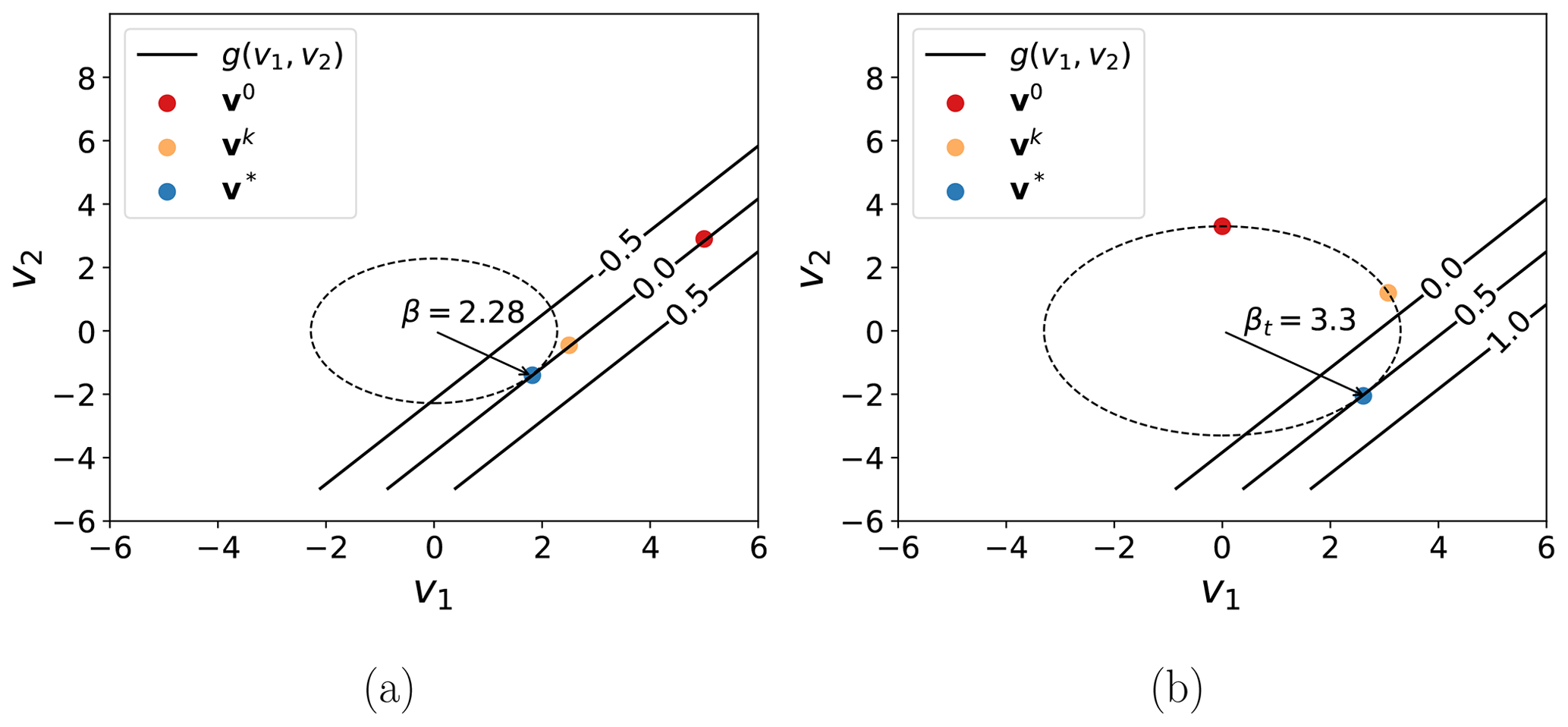
Figure 1The difference between the solutions provided by RIA (a) and PMA (b) for a linear limit state function g with two variables, , in standard normal space. The target reliability index for PMA (βt=3.3) is higher here than the RIA solution (β=2.28), so the PMA solution finds . Also indicated are examples of points visited during the respective optimizations (initial, v0, intermediate, vk, and solution points, v*; different for the two methods), where the displayed points before the solution are feasible but not optimal.
The RBDO problem using PMA can be stated as
where each gj solves Eq. (13) with . One potential downside of PMA is that it does not provide a direct estimate of the probability of failure. This is fine for optimization, where being below the threshold is sufficient and where at least one constraint should be at the boundary where for the final solution. However, if one wishes to compare the probability of failure of such an optimized design with the corresponding initial design or a design optimized by deterministic methods, then PMA does not immediately provide a quantitative answer. It only provides a qualitative assessment of whether or not the probability of failure is above or below the given threshold. To get a quantitative assessment in these cases, we can exploit the approximate linearity of g*, especially close to . If we have solved the PMA problem in Eq. (13) once for a target reliability βt, obtaining the solution g*, we can then use the secant method to construct an estimate of as
where is the solution of a PMA problem for a target reliability . If the initial g* is sufficiently small (close to 0) and/or sufficiently linear, then the above will provide a good estimate β0 and hence an estimate of the probability of failure as . Otherwise, this procedure can be iterated (setting and ). In such cases, unless the initial g* is very far away from zero and/or g is highly non-linear, only a few more iterations (1–3) should suffice to get at least two digits of accuracy for Pf.
2.2.3 Two-loop RBDO vs. single-loop RBDO
As is evident from Eq. (15), the current formulation of the RBDO problem consists of two nested loops. One outer optimization problem that solves the design optimization problem under the given constraints and one inner optimization that solves the (PMA) reliability problem to obtain the probabilistic constraints for each iteration. This can be computationally demanding, even when the convergence of the PMA subproblem is accelerated by the use of improved optimization methods like the hybrid mean-value algorithm (Youn et al., 2003). For this reason, several alternative solution strategies for RBDO have been proposed (Valdebenito and Schuëller, 2010b). This usually involves either decoupling the two loops into a sequence of deterministic optimization and reliability analysis, most prominently in the sequential optimization and reliability analysis (SORA) method (Du and Chen, 2004), or the use of reformulated single-loop approaches, most prominently in the aptly named single-loop approach (SLA) (Chen et al., 1997). All these methods involve some kind of approximation of the FORM-based constraint. While speeding up the convergence significantly compared to conventional two-loop strategies, this can also lead to lack of convergence for some problems (Aoues and Chateauneuf, 2010). On the other hand, SORA seems to be fairly robust, due in large to the fact that its reliability-based constraint is locally equivalent to the two-loop approach, meaning that as the changes in the design become small from one round of deterministic optimization to the next, the error in the approximation when using a fixed reliability estimate during the design optimization tends to zero.
2.3 Surrogate modeling
Surrogate modeling is generally a vast topic and the interested reader is referred to Wang and Shan (2006) and Marsland (2015) for more general overviews, as well as to Tunga and Demiralp (2005) for the high-dimensional model representation approach and Rasmussen and Williams (2006) and Santner et al. (2018) for more detailed looks at Gaussian process regression (GPR). For applications to RBDO in general, Dubourg (2011) and Jin et al. (2003) are instructive.
Focusing our attention to wind turbine applications, it has been common for quite some time to use surrogate modeling due to the computationally demanding simulations required for time-domain analysis. This is especially true for reliability analysis, optimization and RBDO, due to the drastically increased computational effort involved. The most commonly applied types of surrogate models in wind energy have been response surface models (typically second-order polynomials), Taylor expansions and (especially more recently) GPR. GPR has many advantages, including the ability to capture non-linearities with higher fidelity and providing an estimate of its own uncertainty by default but generally requires a larger number of samples to gain a significant advantage over response surface methods (Kaymaz, 2005). We note that GPR is often referred to as kriging in the engineering literature. Although, for most practical purposes, the two terms can be used interchangeably, GPR is more general. Hence, to avoid specificity where it is not needed, we will use the term GPR.
2.3.1 GPR
The essentials of GPR are quite similar to conventional regression methods. We wish to construct a model y(x) for the response y to some input x. However, instead of considering, for example, a multi-linear or polynomial model plus a simple noise term, one instead considers a more general expansion of the input in some basis B (which could be constant, linear, polynomial or otherwise) plus a realization of a zero-mean Gaussian process (GP):
where γ is a set of basis coefficients. The Gaussian process is determined by its covariance function, which is the product of the noise parameter σ and a kernel function. The kernel function gives the covariance function its main structure by determining the correlation between points . Usually, these kernel functions are exponentially decaying with the Euclidean distance between the points. In addition to σ, the covariance function is parameterized by one or more hyperparameters. All in all, GPR consists of fitting γ, σ and all the kernel parameters based on a set of training data {yi,xi}, where in general each input xi can be multi-dimensional. These parameters are fit using maximum likelihood estimation, though finding optimal parameters often requires the use of global optimization methods in order to fully consider the range of possible parameter values. The fitted covariance function of the GPR model, in particular the value of σ, provides a natural estimate of the inherent uncertainty (or expected error) of the surrogate model, which can then be used to establish confidence/prediction intervals for predicted model responses to new inputs. An illustration of GPR is given in Fig. 2.
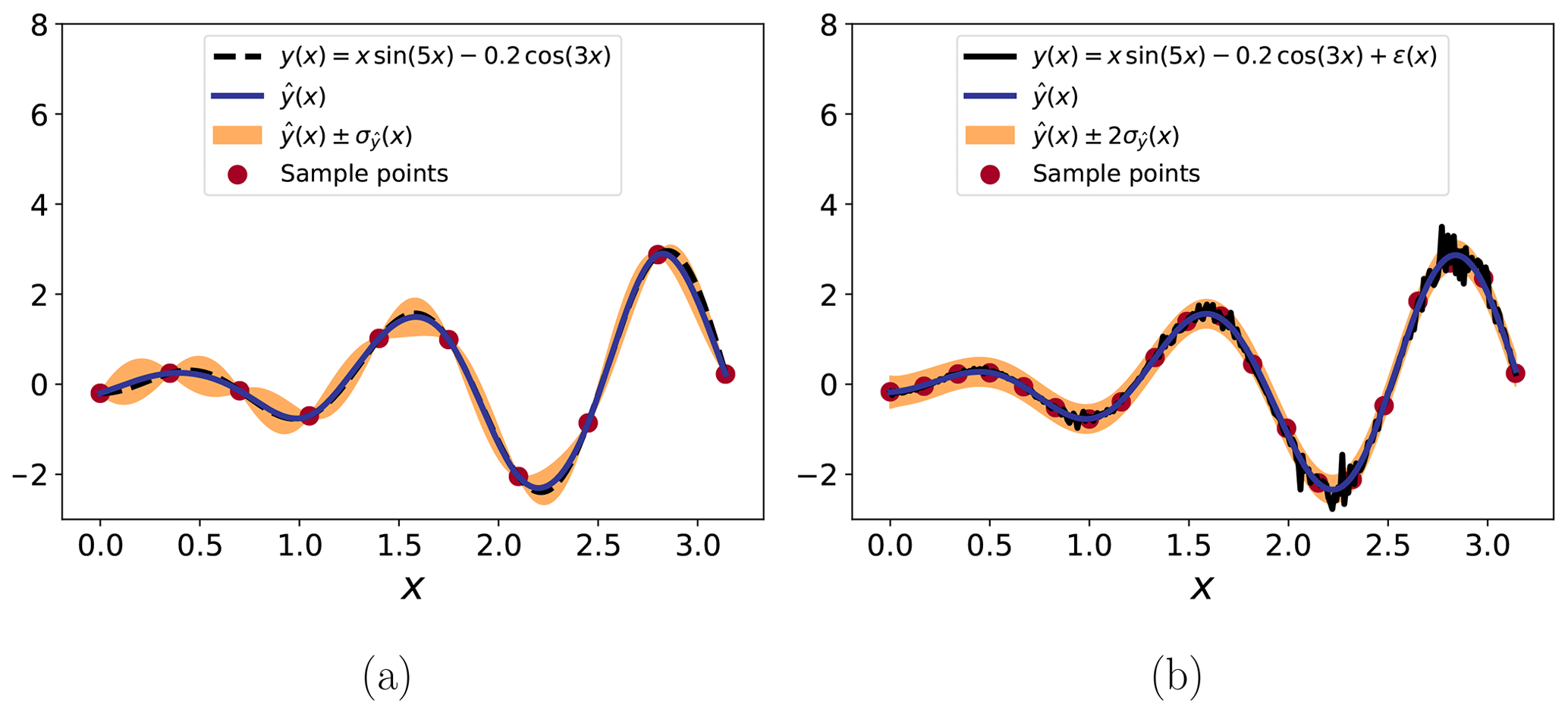
Figure 2GPR demonstrated on two related test functions: one with no noise (a) and one with noise (b). In the former case, 10 sample points are enough for a very good estimate (the real function, y, being within 1 standard deviation of the estimate, , throughout). Note also how the uncertainty decreases around the sample points in this case due to the lack of noise. In the second case, more samples are needed for a good estimate. The noisy function does at one point exceed even 2 standard deviations away from the estimate, but the underlying (non-noisy) function is well estimated. Note also how the uncertainty level, while more or less constant, is not higher than it was away from the sample points of the non-noisy case.
2.3.2 Design of experiment
As noted previously, GPR can require a large number of samples to attain its desired fidelity. For this reason, it is common to apply specialized sampling techniques, together usually referred to as the design of experiment (DOE), that sample the input space more efficiently and thereby require less samples than, e.g., uniform random sampling. Depending on the desired outcome, one could, for instance, opt for importance sampling (most useful in this case if it is known that only a certain region of the input space is of interest, e.g., for a reliability analysis where one mainly wishes to use the surrogate model around the failure surface) or a space-filling approach like Latin hypercube sampling or quasi-Monte Carlo sampling (these are most useful when as wide coverage of the input space as possible is needed, e.g., for optimization where the region of interest is likely to shift dynamically). A comparison between Latin hypercube sampling and quasi-Monte Carlo sampling was performed in Kucherenko et al. (2015), where it was found that Latin hypercube sampling can give better or more efficient results for certain types of problems but that quasi-Monte Carlo sampling was otherwise equal or superior and generally more robust when the problem could not be classified a priori. Latin hypercube sampling has been more common for wind energy applications, but a quasi-Monte Carlo sampling method based on the Sobol sequence was used in Müller and Cheng (2018).
2.4 Proposed RBDO framework
In the following, we will explain the details of our proposed framework for RBDO of OWT support structures. However, we begin with a few remarks that serve to motivate this approach.
2.4.1 Motivation
Considering the state of the art for reliability analysis and RBDO for OWTs more generally, we can make a few summary observations based on the previous discussion. Firstly, the vast majority of studies make use of either simplified analytical limit state functions (allowing more easily the use of FORM and making the probabilistic constraints easier to combine with design optimization) or surrogate models that completely replace simulation output (usually combined with sampling-based reliability analysis). Secondly, when not based on heuristic optimization methods (as has been the case for all RBDO studies concerning the design of support structures specifically), gradient-based design optimization as part of RBDO has not utilized analytical sensitivities. Thirdly, little to no use of PMA for reliability analysis or more advanced RBDO methods like SORA or SLA has been made, despite their notable advantages.
What can be concluded from this? Simply put, considerable progress could be made by making the state of the art for OWT RBDO, and for support structure design in particular, more in line with the general state of the art. However, this should be done in a way that maintains some of the OWT-specific developments made in previous optimization studies. Furthermore, by combining elements from all these sources, it could be possible to obtain a synthesized methodology that retains many of the individual advantages. However, this requires a new approach because of the ways in which the previous methods seem incompatible. It is, e.g., seemingly not possible to use analytical sensitivities if the simulation output is replaced by surrogate models.
2.4.2 Key simplification
Suppose that all relevant limit state functions gj can be written in the form , which is generally the case for support structure design, with Q and R being the load effect and resistance as before. Furthermore, for simplicity (and since this is usually the case), assume that while both Q and R are functions of the design x and the stochastic variables θ, only Q is determined by simulations. We then make the following simplification:
where Y is some arbitrary unknown function with the property that , with as the mean values of θ, and is the mean response at the specific design x. A simple example of how such a factorization makes sense locally is shown in Fig. 3. What are the implications of this assumption? Firstly, note that this assumption is consistent with the common simplified limit state functions where the stochastic response is modeled as the product of the stochastic variables θ and the design-dependent mean response. However, in our case, we make no assumption about the functional representation of this factorization. Hence, this should allow for a higher-fidelity representation of how stochastic variables input to the system are propagated through the response estimation. Secondly, while this is indeed a simplification which cannot in general be assumed valid, previous studies detailing how the fatigue damage distribution of OWT support structures changes when the design is modified (Stieng and Muskulus, 2018, 2019) indicate that this kind of proportional scaling is a reasonable assumption as long as the design does not change too much. Furthermore, it is not unreasonable to make a similar assumption for extreme loads. Thirdly, this factorization makes it possible to fit a surrogate model of the response to variations in the stochastic variables only, while the design-dependent part of the response remains as in a deterministic setting. On the one hand, this means that we can fix the design and fit our surrogate model as
where for each sampled point θs we estimate the total response Q and then factor out the design-dependent mean response. This greatly reduces the dimensionality of the surrogate modeling problem, since we do not have to also sample different values of x. Since the fit is design independent given the underlying simplifications, we may then say that we obtain a quasi-global (in design space) surrogate model that can be used throughout a design optimization procedure, greatly reducing the computational effort of any reliability calculation. On the other hand, the separation of stochastic and deterministic response means that for the estimation of design sensitivities we have the property that
Hence, the use of analytical design sensitivities becomes possible. Finally, note that while the simplification is expected to lose accuracy as the design moves further and further away from the initial configuration where the surrogate model was fit, the mean response remains exact. This is not the case when a surrogate model fit replaces the simulated response entirely. Hence, for use in RBDO, the factorization in Eq. (18) is going to behave at worst like a deterministic optimization that includes some simplified reliability estimate (based on Y) that modifies both the constraint value and the constraint gradients, in a way not too different from SORA and SLA.
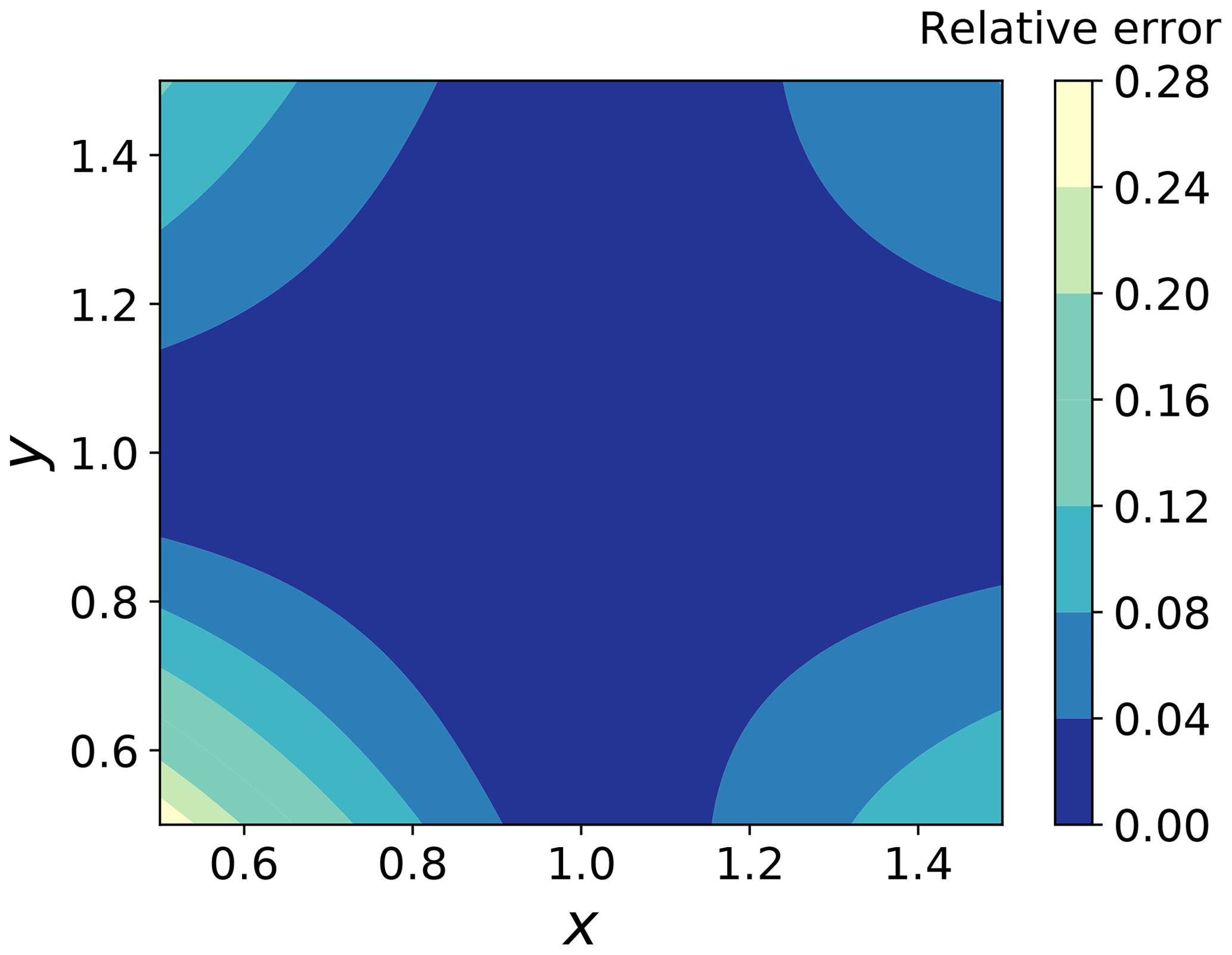
Figure 3An example of factoring out the dependence of one variable from a non-separable expression by using GPR to fit this unknown factor. The figure shows the relative error when approximating (x+y)2 as f(y)(x+1)2, around x=1, with f(1)=1 and otherwise unknown. Note the accuracy of this representation around (1,1) and in general the moderate error level as we move away from this region.
2.4.3 Formal statement
Our overall proposed framework is based on the previously stated PMA-based RBDO problem in Eq. (15), restated here for convenience:
gj is now defined as
with yj as a surrogate model defined and fit according to Eqs. (18) and
(19), and θq and θr are the stochastic parameters in θ for the load effect
and the resistance, respectively. Note that we can obtain , so that even though
the solution of the reliability subproblem resulting in v* is performed in standard normal space, it is
never necessary to obtain yj as a function of v. To ensure that the RBDO problem is solved with sufficient
accuracy, specifically that the final design is actually feasible with respect to the probabilistic constraints, the
procedure can be repeated several times, fitting a new surrogate model at the solution of the previous RBDO loop and
starting a new RBDO loop from this design point. The overall method is compactly stated as Algorithm 1
and illustrated in Fig. 4.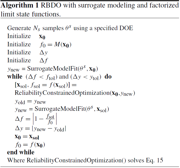

The design optimization performed in this study will in all cases be based on output from time-domain simulations of finite element models. These have been implemented in an in-house, MATLAB finite element code as assembled Timoschenko beam elements with 6 degrees of freedom at each end of each element. The analysis is based on Newmark integration and uses a consistent mass matrix and a Rayleigh damping matrix with mass and stiffness proportionality scaled according to the first two eigenmodes. A typical finite element, including variables, is shown in Fig. 5a and a more general representation of the OWT system is shown in Fig. 5b.
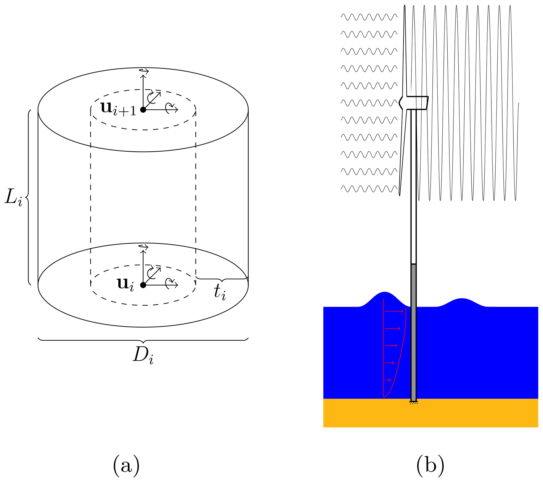
Figure 5Beam element with design variables (Di,ti), length Li, nodal coordinates u and coordinate systems indicated (a) and the offshore wind turbine system and environment (b).
3.1 Models and loads
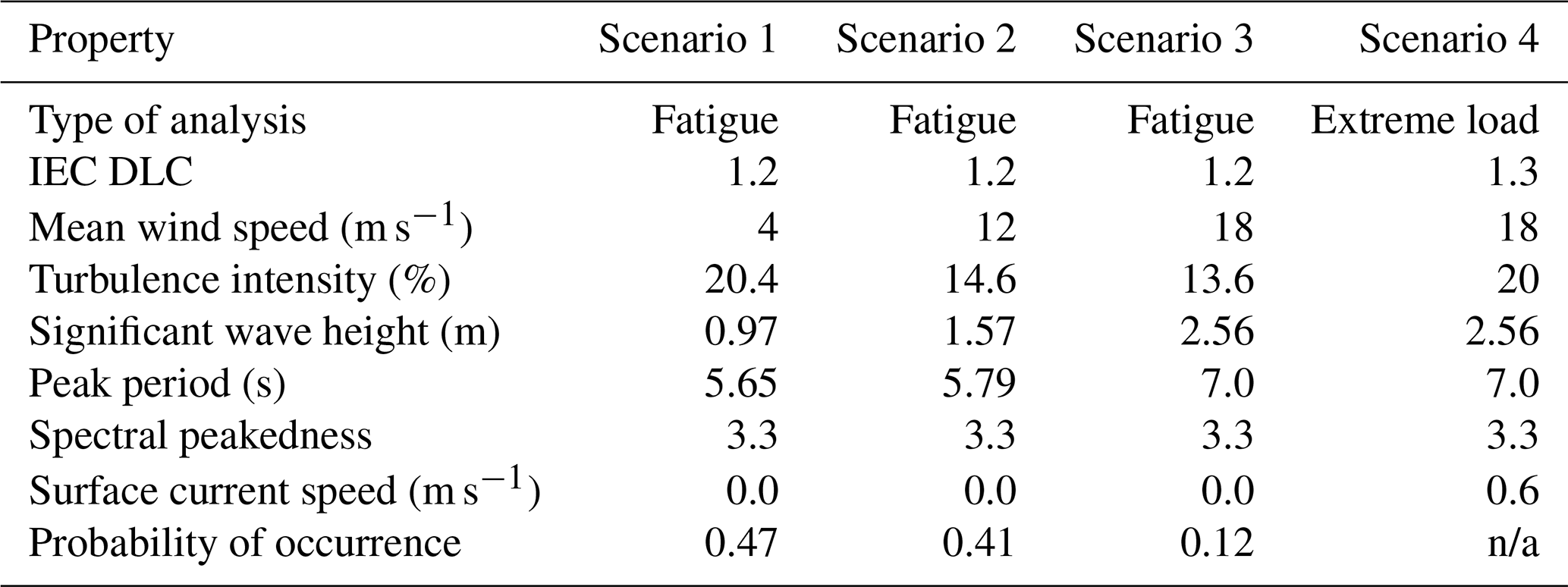
To test the proposed methodology, two main cases will be used. The first of these cases is a simplified model based on a uniform section of a monopile support structure, initially uniform in its cross-sectional dimensions and with uniform lengths for each element. This is meant to demonstrate the basic idea of the method without having to consider realistic designs. This model will be referred to below as the “Simple Beam”. The second case is a simplified but reasonably realistic representation of the OC3 Monopile (Jonkman and Musial, 2010) with the cross-sectional dimensions of each segment initially corresponding to the OC3 design, i.e., with a uniform monopile segment and a linearly tapered tower segment. The element lengths are consistent within each major segment but differ between the tower and monopile. Furthermore, this model also includes a point mass on the top of the tower, with mass and inertia properties meant to represent the National Renewable Energy Laboratory (NREL) 5 MW turbine (Jonkman et al., 2009). This model will be referred to as the “OC3 Monopile”. Some of the basic properties of these two models are listed in Table 1, and the material properties are consistent with the ones in Jonkman and Musial (2010). The models are fixed (clamped) at one end (at a location that corresponds to the mudline for the OC3 Monopile); i.e., there is no modeling of soil included. This will affect the global stiffness and change the dynamics of the structural models somewhat but is not expected to have a large effect on how these models function in terms of testing the RBDO method. Both models are loaded at the top with force and moment time series extracted from fixed rotor simulations of the NREL 5 MW turbine subject to turbulent wind fields within the aeroelastic Fedem Windpower software (Fedem Technology, 2016). Note that the externally input rotor loads are only calculated once and are taken as design independent, though the response to these loads is calculated for every design. These forces and moments are input into the dynamic simulation as loads on each of the 6 degrees of freedom on the top node of the tower. Wave loads are represented by a horizontal force time series, applied at a location corresponding to the bottom of the tower in the OC3 Monopile and at an analog location for the Simple Beam. In the dynamic simulation, this is input as a load on the degree of freedom corresponding to displacement in the mean wind direction, but no other degrees of freedom are loaded by this force. This force has been tuned to give an equivalent moment at the lower end of the structures as the integrated contribution of all horizontal wave forces along the height of the water column at each instant in time. These forces are calculated from the Morison equation, based on wave kinematics sampled from the Joint North Sea Wave Project (JONSWAP) spectrum and including Wheeler stretching. The inertia and drag coefficients are 2.0 and 0.8, respectively. Since the wave loads depend on the diameter of the relevant members, these loads are recalculated for every design before being input to the dynamic simulation. The duration of the applied loads is 600 s after the removal of initial transients. Up to four different loading scenarios are included in the analysis, with environmental data based on the Ijmuiden Shallow Water Site (Fischer et al., 2010) and using different random seeds for each realization of wind and wave conditions. The probabilities of occurrence for fatigue estimation have been renormalized so that they sum to 1 for the reduced set of cases. These loading scenarios are summarized in Table 2.
Table 1Properties of the two models used in the study.
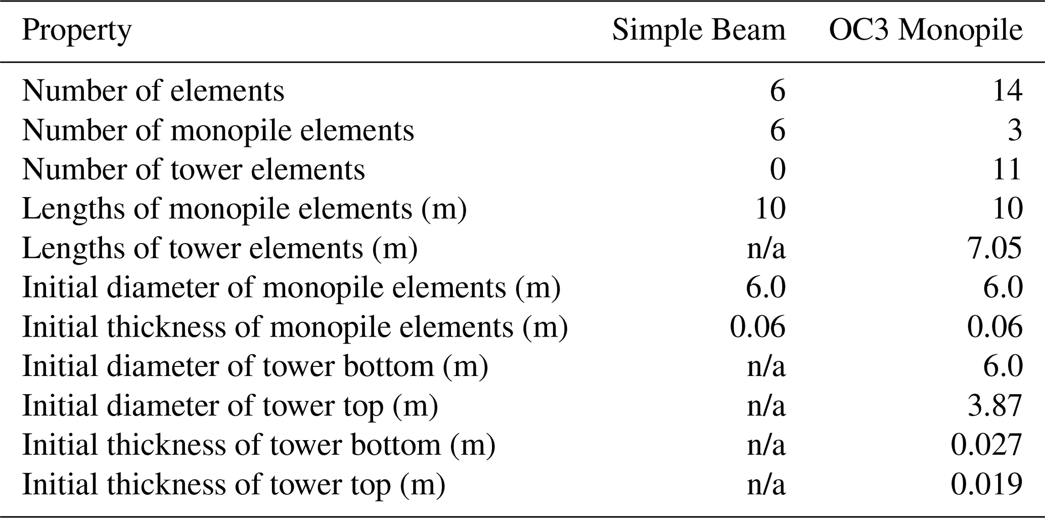
n/a – not applicable.
Table 2Properties of the loading scenarios. International Electrotechnical Commission (IEC) design load cases (DLCs) refer to International Electrotechnical Commission (2009).
3.2 Constraints
As indicated in Eq. (15), the optimization is constrained with upper and lower bounds on the design variables. This is done from a theoretical point of view in order for the final designs to be somewhat realistic with respect to practical constraints related to manufacturing, transportation and installation that are not specifically accounted for in the modeling. From a more practical point of view, some decreased numerical performance was observed, during initial testing, once the design variables went outside a certain range, especially for certain combinations of values for some variables. For this reason, the upper and lower bounds were set stricter than normal practice would dictate. In particular, the lower bounds are for both models set at 70 % of the smallest initial diameter and thickness, respectively; the upper bounds are set at 150 % of the largest diameter and thickness, respectively. We refer to Table 1 for the smallest and largest values for each model. While these bounds do not directly correspond to any specific real limits, the restriction is not expected to rule out any design of practical interest. As for linear constraints, we will in some cases include an upper limit on the D−t ratio of 120, consistent with the NORSOK standard (Standards Norway, 2013). In terms of non-linear constraints, we consider limits on the accumulated 20-year fatigue damage and on the maximum bending moment, to be detailed below. Fatigue calculations are done as follows. From the displacements obtained as the solutions to Eq. (3), the internal forces and moments Sin are obtained by multiplication with the element stiffness matrices Ke as
From the components of Sin corresponding to the axial force Sax, in-plane and out-of-plane moments Sip and Sop, the normal stress σn is then identified as
where is the cross-sectional area and is the second moment of area. Rainflow counting (Rychlik, 1987) is then applied to the normal stress time series, resulting in a set of amplitudes Δσi that correspond to the differences between stresses at particular times (a stress cycle), encoded in the vectors tpeak and tvalley, i.e.,
Unlike what is otherwise common practice, these amplitudes are not binned. This is in order to facilitate the sensitivity analysis. The incurred fatigue damage F is then estimated by use of the Palmgren–Miner linear summation rule, where the contribution from each stress cycle is given by application of the appropriate SN curves and thickness correction (Det Norske Veritas, 2016):
where ni is either 0.5 or 1.0 depending on whether the given cycle is a half or full cycle, ai is a constant, wi is the Wöhler exponent, tref is the reference thickness below which no correction is necessary, and k is the thickness correction exponent. The constants ai, wi, tref and k are set using the SN curves for welds in tubular joints (in air and in water with corrosion protection, respectively, depending on the element) found in Det Norske Veritas (2016). The total lifetime fatigue damage, Ftot, from all considered environmental states, E, is then
where Tlf is a factor scaling up from simulation time to a 20-year lifetime, F(E) evaluates Eq. (25) for each state, E and Pocc are the corresponding probabilities of occurrence for these states. The limit state function for fatigue, measuring the extent to which the lifetime fatigue damage exceeds the fatigue resistance ΔF (usually set to 1), used as a constraint in the deterministic optimization problem, is hence
For the maximum bending moment, the calculation is based on Sip as obtained from Eq. (22). However, since the use of global maxima can cause problems with smoothness (the global maximum may not always change smoothly) and since checking the bending moment at every time step would be very time consuming, a compromise is made. In particular, the Kreisselmeier–Steinhauser function (Kreisselmeier and Steinhauser, 1979) is used to smoothly aggregate the bending moment time series into an upper envelope of the maximum:
where the subscript max denotes the global maximum, and r is a constant controlling the accuracy of the approximation. The above expression approaches Sip,max from above as r approaches infinity. For computations, r is typically taken to be 50–200 (set to 200 here) depending on desired accuracy (see Couceiro et al., 2019 for a discussion of this for OWT applications). Note that, algebraically speaking, Sip,max cancels out1. Taking Eq. (28) as an estimate of the maximum bending moment, we then compare this with the NORSOK design criterion for tubular members subject to bending (Standards Norway, 2013). The calculation for the bending resistance uses the one for a D−t ratio of 120 (for realistic D−t ratios exceeding this value, the changes are negligible). The resulting limit state is
where is the plastic section modulus, γM is the material factor and fy is the yield strength of the material. The material factor is fixed at 1.45.
In principle, many other types of constraints should be included in order to ensure that the structure adheres to safety standards (e.g., buckling) and having constraints on eigenfrequency (to avoid dynamic amplification) is also common. However, in order to focus our attention on how the basic support structure optimization problem is affected by the presence of probabilistic constraints, and see the effect of each probabilistic constraint more clearly, these other safety checks have been left out.
3.3 Sensitivity
The estimation of gradients for the objective function as given in Eq. (2) and the linear constraints is trivial. For the non-linear constraints, it is mainly a question of repeated application of the chain rule as well as the rule of total derivatives for multivariate functions. See, e.g., Chew et al. (2016) for details of how this can be done (the only modification in our case being the additional level added by Eq. 28, which is easily differentiated). However, note that, due to how the displacement sensitivity is calculated in Eq. (4), regardless of location in the structure, there is always a dependence on each design variable for every non-linear constraint. Hence, none of these derivatives are zero in general.
3.4 Probabilistic aspects and uncertainty modeling
For the RBDO formulation based on PMA, the limit state functions represented by Eqs. (27) and (29) can be directly used, with the understanding that Ftot, Δf, MKS and fy become probabilistic quantities. Using the notation in Eq. (21), we have
where, for simplicity, we define and . The sensitivities then follow from Eqs. (14), (20) and the above discussion. In this study, a target reliability index of βmax=3.3, corresponding to , will be used for the solution of the PMA subproblem in Eq. (13) as part of Algorithm 1. The uncertainties that are included in the response are global stiffness, global damping and turbulence intensity. The uncertainty modeling will be detailed below.
3.4.1 Global stiffness
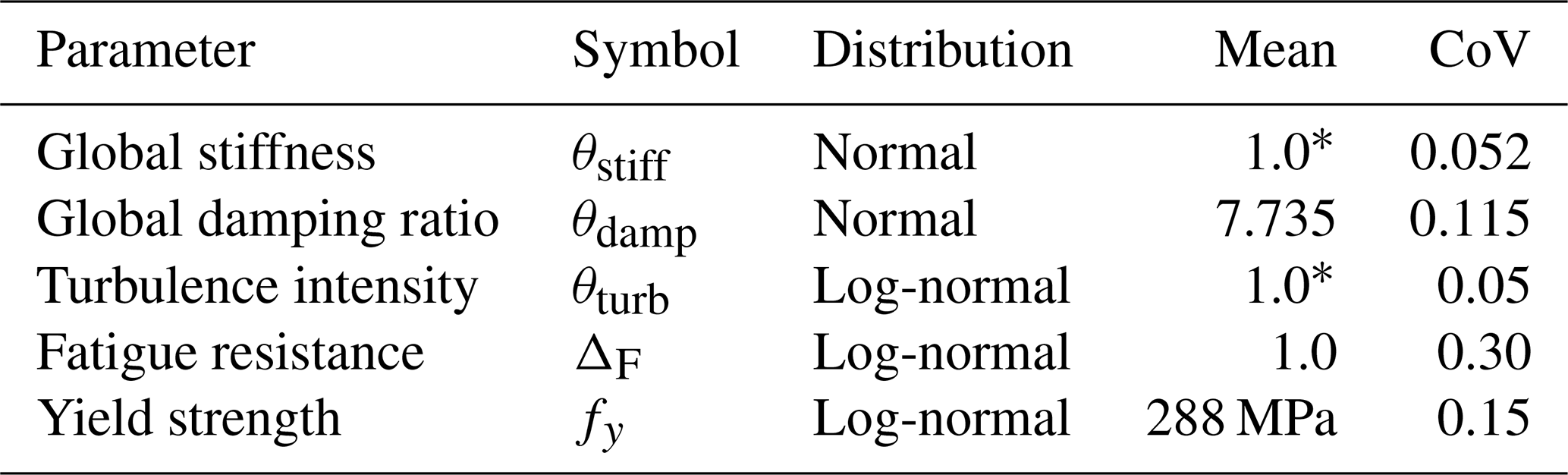
The uncertainty in stiffness is assumed to come from uncertainty in soil stiffness. Though no soil modeling is included in the present analysis, this mainly introduces a shift of the mean stiffness, and hence one may still consider the impact of a stochastic uncertainty in the soil stiffness. The effect of soil pile stiffness on the fundamental eigenfrequency of a monopile was discussed in Kallehave et al. (2015). The expected range of the fundamental frequency was found to be [0.937,1.045] as a ratio of its mean value. If we symmetrize this as [0.94,1.06] and use the fact that global stiffness of a monopile is proportional to the square of the fundamental eigenfrequency, we can then obtain the expected range of global stiffness as [0.88,1.12] as a ratio of its mean value. Taking this to be a 98 % confidence interval and, for lack of other information, assuming that the uncertainty in global stiffness follows a normal distribution, we obtain that , i.e., a coefficient of variation (CoV) of 0.052. As an independent confirmation, this is close to, if a bit higher, than what would be obtained from Andersen et al. (2012) and Damgaard et al. (2015) (each giving a coefficient of variation of about 0.04).
3.4.2 Global damping
For the uncertainty in global damping, the two main contributions are assumed to come from aerodynamic damping and soil damping. Expected ranges of the damping coefficients corresponding to these two sources can be obtained from Chen and Duffour (2018) as [4.0,8.0] for aerodynamic damping (in the fore–aft direction for operational conditions) and [0.17,1.30] for soil damping, both given as percentages of critical damping. Assuming, as above, that these ranges correspond to 98 % confidence intervals and that the uncertainty can be modeled (for lack of better knowledge) as following a normal distribution, then we obtain and . Summing these contributions and adding also a constant (deterministic) structural damping of 1.0, the final result is , a CoV of 0.115. The soil uncertainty obtained here is about the same as would be derived from Damgaard et al. (2015). The aerodynamic damping is harder to verify with additional sources, and in principle the level of uncertainty is expected to be wind speed dependent. For lack of more detailed knowledge, the present values are used in this study.
As a small comment, we have so far assumed both stiffness and damping to follow normal distributions. It has been common practice in previous studies to model uncertainties related to soil and aerodynamic damping as log-normally distributed (sometimes other skewed distributions). However, at a CoV of 0.05, there is almost no difference between the corresponding normal and log-normal distributions. Even with a CoV of 0.12, the differences are fairly small. See Fig. 6 for details. Hence, the impact of this simplification is minor.

Figure 6Normal distribution vs. log-normal distribution sharing mean and standard deviation: mean 1.0 and standard deviation 0.05 (a); mean 1.0 and standard deviation 0.12 (b).
3.4.3 Turbulence intensity
The turbulence intensity is modeled as log-normally distributed with a wind speed-dependent mean and a CoV of 0.05, i.e., , with m derived from Table 2. This is consistent with, e.g., Sørensen and Tarp-Johansen (2005), Veldkamp (2008) and Toft and Sørensen (2011). The particular value is based on the expected uncertainty in turbulence intensity as derived from the uncertainty of cup anemometer measurements. If including also the uncertainty from wake modeling in a wind farm, which is not done here, the CoV will be higher (Toft et al., 2016b).
3.4.4 Fatigue resistance and yield strength
The fatigue resistance is modeled as log-normally distributed with a mean of 1.0 and a CoV of 0.3, consistent with, e.g., Márquez-Domínguez and Sørensen (2012) and Toft et al. (2016b), i.e., .
The yield strength is modeled as log-normally distributed with a mean of 288 MPa and a CoV of 0.1, consistent with, e.g., Melchers (1999). To account for some of the effects of the simplifications used to arrive at Eq. (29), the CoV is increased to 0.15. Hence, .
The uncertainty modeling is summarized in Table 3.
Table 3Uncertainty modeling details. Quantities marked with * are expressed relative to the respective deterministic values.
3.5 Implementation details
So far, some of the details of the proposed methodology have been left unspecified in order to suggest an overall framework for RBDO rather than a very specific set of methods. The literature contains a large amount of choice in regards to optimization algorithms (both at the design optimization level and in the inner optimization loop solving the reliability problem), surrogate modeling and DOE. While these details have to be fixed in order to demonstrate the method in practice, the optimal selection of algorithms is not considered within the scope of the present study. Such optimality will in any case be both application specific and depend on the personal preferences of the designer.
With regards to both levels of the optimization, we use a combination of SQP and interior-point methods (Nocedal and Wright, 2006), both of which are common examples of gradient-based non-linear constrained optimization algorithms. In principle, the PMA-based reliability problem can be solved more efficiently by use of the hybrid mean-value method (Youn et al., 2003) or related approaches, but due to the use of the surrogate model, this is not deemed necessary for the current application. Convergence of the optimization is based on fairly standard criteria, with termination of the algorithms when either relative first-order optimality (see, e.g., Nocedal and Wright, 2006) is achieved with a tolerance of 10−6 or the relative changes in the design variables are less than 10−6. Solutions are required to be feasible with a tolerance of 10−6.
For the surrogate modeling, we have chosen GPR due to the benefits stated previously. After some initial trial and error, the Matérn class kernel with was chosen, including the use of individual length scale hyperparameters for each input variable (this implements what is known as automatic relevance determination, in principle de-emphasizing less relevant input variables in the regression problem; see, e.g., Rasmussen and Williams, 2006). Overall, this was found to be the most robust for the regression problem in this study, especially when considering repeated regression for additional iterations of the outer loop in Algorithm 1. The Matérn class of kernels was also used for OWT support structures in Häfele et al. (2019). We also note here that in order to simplify the simultaneous regression with respect to all of the three parameters in θq, these parameters were input to the fitting problem in such a way that the surrogate model became co-monotonic in every variable (an increase in one or more variables giving always an increase in the output). In this case, that meant inputting the inverse (1∕θi) of the parameters controlling damping and stiffness. Furthermore, these parameters were implemented as scaling variables with means of 1.0, such that the actual variables as input to the simulations were a product of the deterministic values and the respective stochastic scaling parameters in θq. The hyperparameters of the Gaussian process model were fit using Bayesian global optimization methods (expected improvement) (Mockus, 1975; Jones et al., 1998; Brochu et al., 2010). The noise standard deviation was taken to be non-zero and also fit during this procedure, even though the simulation outputs used in the fitting are in a certain sense noise-free. This was done because it was seen to give more robust surrogates with respect to changes in the design.
The DOE was done using Sobol sequences, a quasi-Monte Carlo method. This has the advantage of being more space-filling, covering a larger range of the space while still having some clustering to account for local variations, compared to many ordinary Monte Carlo methods. While not made use of here, Sobol sequences also have the advantage compared to the commonly used Latin hypercube sampling method that it is much easier to interactively add new samples to the old set. To this last point, the use of an adaptive DOE was not used here, despite this increasingly becoming the common approach for GPR. The main reason why was a practical one, having to do with the way the loading input was sampled, which made interactively adding samples during a fitting procedure difficult for our implementation. A total number of 500 samples were pre-generated, with the number of samples actually used increasing for each iteration of the outer loop in the following way. For the initial surrogate model, 50 samples were used. The new model at the solution of the first RBDO procedure was then trained with 100 samples and compared with the old model using 25 additional samples, for a total of 125 samples used. All subsequent iterations use the full set of 500 samples, with 400 used for training and 100 for comparing the current model with the previous one. In a sense, the DOE is thus somewhat dynamic, even if it is not adaptive.
Finally, the outer loop needs termination criteria, as indicated in Algorithm 1. One such criterion was chosen to be simply the convergence of the objective function value. Once this value changes less than a certain small tolerance, the outer loop was halted. However, it is possible to terminate slightly earlier if the surrogate model is seen to converge, since in that case the objective function will not change significantly or at all during the next iteration. As implied above, the new surrogate models trained at the solution of the current RBDO loop were thus compared with the models used during that loop. Due to the use of noisy regression models, the surrogate models will in practice never converge entirely (or will at least do so very slowly) as long as there are small changes in the design (and small changes in the surrogate model give further small changes in the design, etc.). Hence, a more relaxed convergence criterion was developed for the surrogate models. Specifically, if we denote by and , the mean prediction of the new and old surrogate models, respectively, and by σy,old, the predicted standard deviation of the old model, then if
for every test sample point, the surrogate model is not updated. If no surrogate models are updated after an outer iteration, the procedure terminates. In order for this relaxed tolerance not to give infeasible results with respect to the new surrogate model (which is not used when it is within the above tolerance), the surrogate predictions for y(θq), used to compute the numerical values for the limit state functions in Eqs. (30) and (31), are based on the mean plus the standard deviation, , rather than just the mean. This guarantees that when is used instead of the updated model, the derived results remain strictly feasible with respect to mean of the more accurate prediction (which would otherwise have been used). Since the standard deviations tend to be , this does not have a large impact on the results.
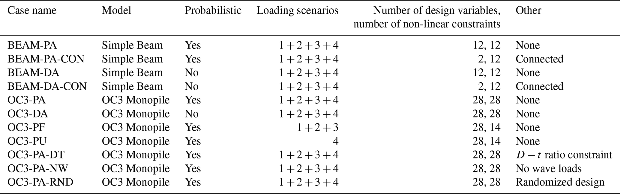
To illustrate both the basic workings of the RBDO method and the effect of certain modeling choices and constraints, a number of different cases are studied. For easy reference, these have been given names and will be referred to as such from now on. The names and properties of each of these cases are listed in Table 4. Note that for cases marked with “connected”, only one set of values for diameters and thicknesses is used throughout the structure, meaning there are only two design variables. In all other cases, there is one diameter and thickness per element (giving 12 design variables for the Simple Beam model and 28 for the OC3 Monopile). There is also one set of non-linear constraints (fatigue, extreme load or both) per element. To make comparisons between deterministic and probabilistic optimization more clear, the deterministic non-linear constraint limits have been tuned to match more closely their probabilistic counterparts. In particular, the deterministic versions of the resistance variables ΔF and fy have been set to for and , respectively. This can be considered a form of simplified safety factor scaling.
Table 4Testing cases for RBDO. Loading scenario numbers refer to the values in Table 2.
4.1 Simple Beam
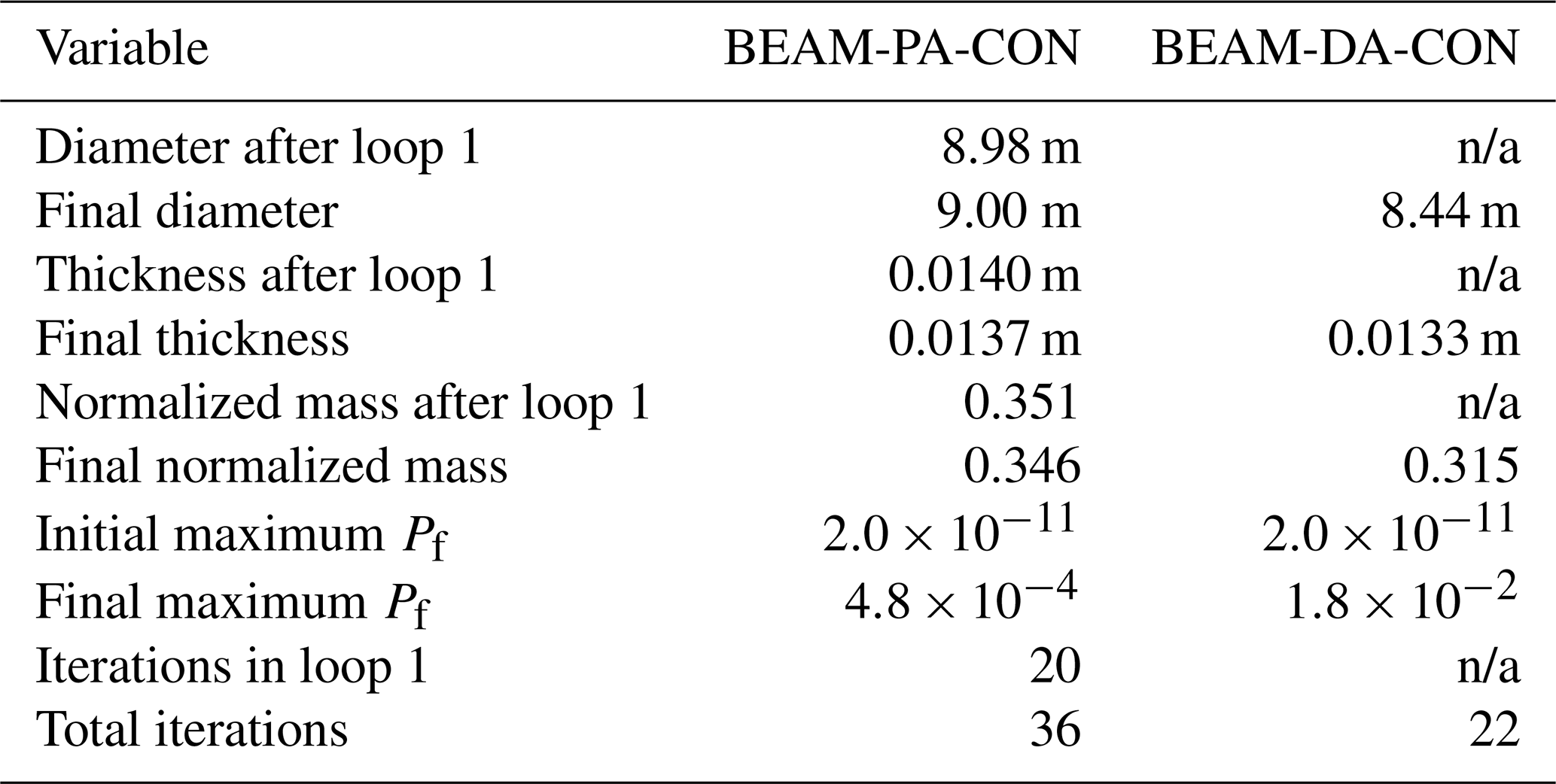
The objective function for case BEAM-PA-CON is shown in Fig. 7a. Note how there are only very minor changes after the first loop. The small modifications to the design variables in the second and third loops are caused by the updates in the probabilistic constraints, seen in Fig. 7b. The final design is characterized by an overall minimization of thickness while the diameter is increased, as seen in Fig. 7c. Comparing with the corresponding deterministic case BEAM-DA-CON, the main difference is a slightly more conservative design, as would be expected. The corresponding plots are not shown, as they are almost identical, but results for both cases are summarized in Table 5. Note that the amount of outer iterations for loop 1 of BEAM-PA-CON is about the same as the total number of iterations for BEAM-DA-CON.
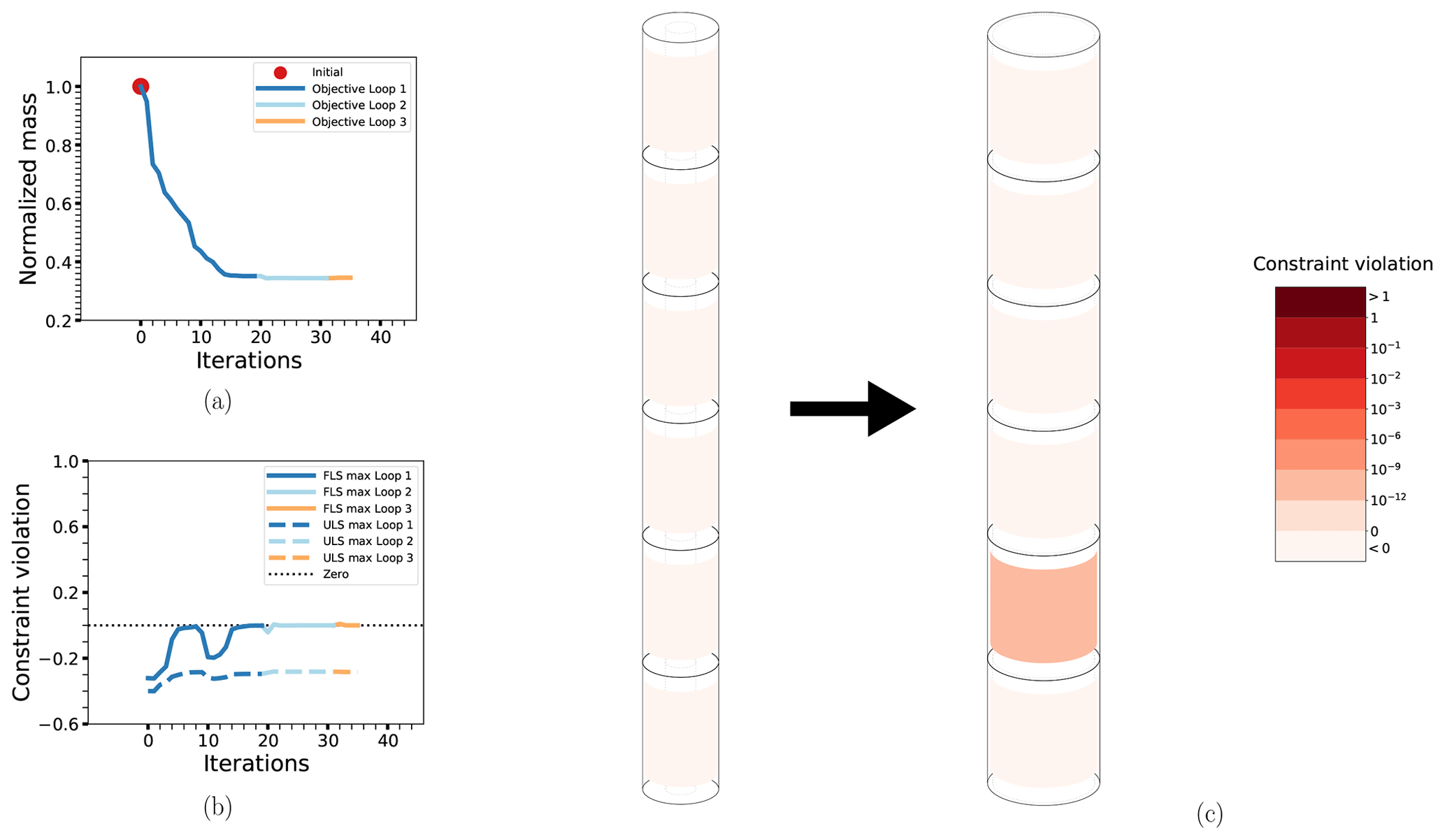
Figure 7The optimization process for case BEAM-PA-CON: the objective function (a), maximum non-linear constraint violations (b) and the change in the design from initial to final configuration (c). The design drawings also have the level of non-linear constraint violation indicated by the coloring of the elements. The thicknesses have been exaggerated for legibility.
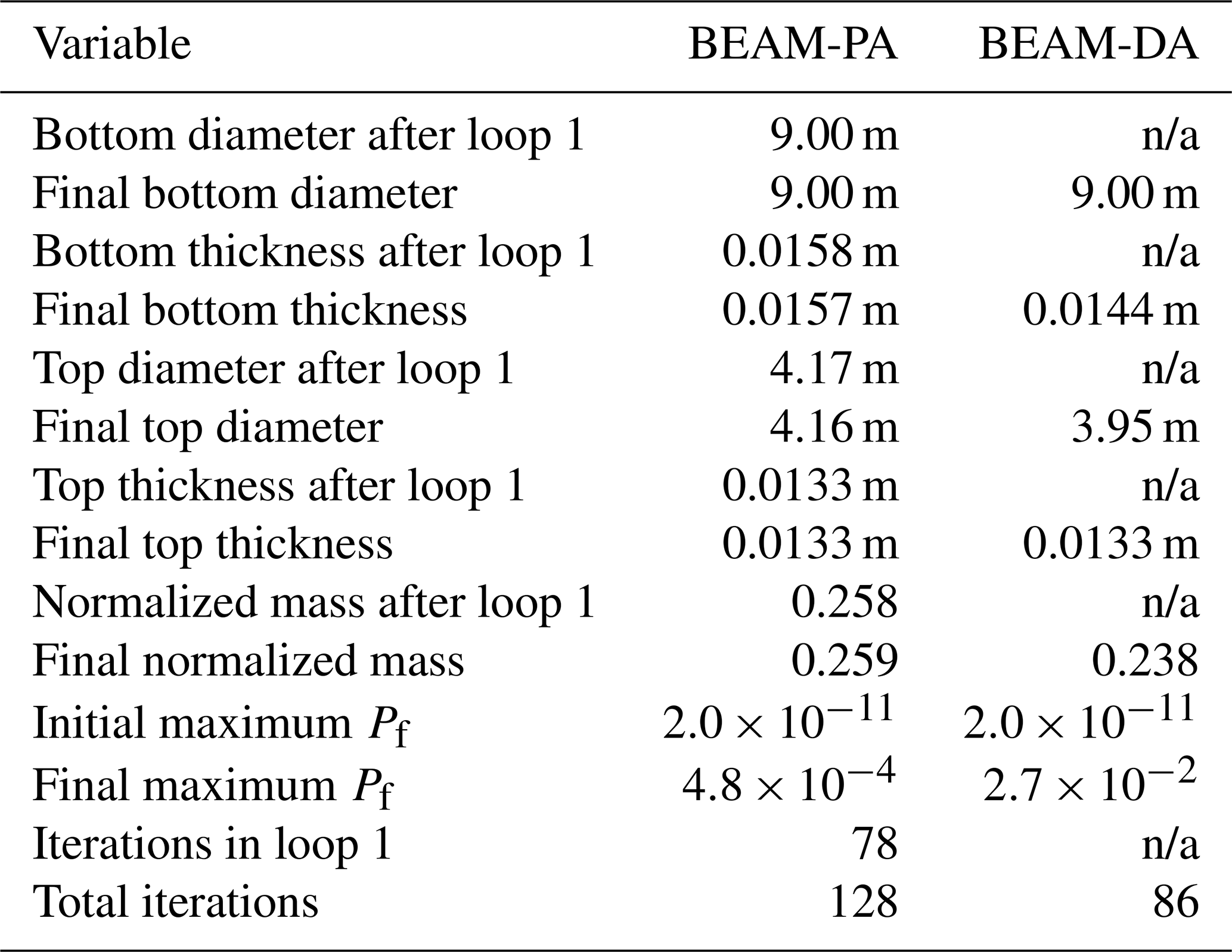
The results for BEAM-PA and BEAM-DA are shown in Figs. 8 and 9, respectively. Compared to the cases with connected design variables, there is an (expected) increase in the number of iterations required to solve the problem, and the resulting designs are different in the way that the dimensions are reduced for elements higher in the structure. This is a natural consequence of the fact that the loads are higher towards the bottom and the constraints there will be stricter in terms of allowable cross-sectional dimensions. Otherwise, the results are similar. The non-linear constraints are somewhat closer to being active at the solution of the RBDO problem compared to the deterministic case, which was true previously but is more apparent for these cases. Detailed summary results are for these cases displayed in Table 6.
All in all, the results so far show that the method works well for these simple systems. The convergence behavior is more or less as for the deterministic case, with the addition of a few short extra loops to achieve overall convergence with respect to the updated GPR-based surrogate model. However, the results obtained from the first outer loop are likely good enough for practical purposes. The fatigue constraints dominate over the extreme load constraints, which is not unexpected. Furthermore, the system seems driven by the thickness(es) both with respect to the objective (structure mass) and the (fatigue) constraint, and the solutions reflect this (with minimal thicknesses and increased diameters where necessary to compensate). This can mostly be understood as a result of the fact that the contribution of the thickness to the cross-sectional areas and second moments of area is of higher order than that of the diameter.
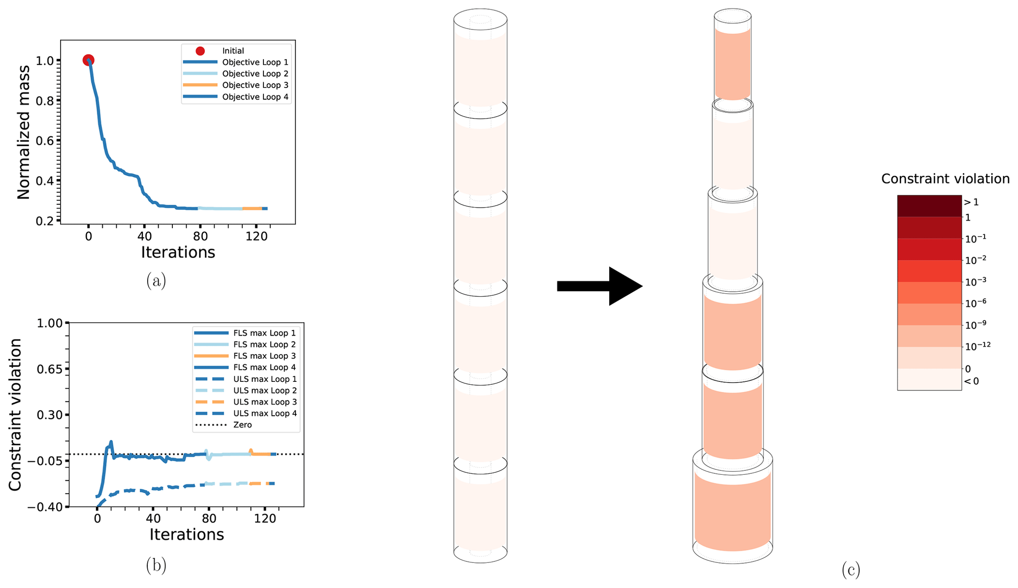
Figure 8The optimization process for case BEAM-PA: the objective function (a), maximum non-linear constraint violations (b) and the change in the design from initial to final configuration (c). Details as in previous figure.
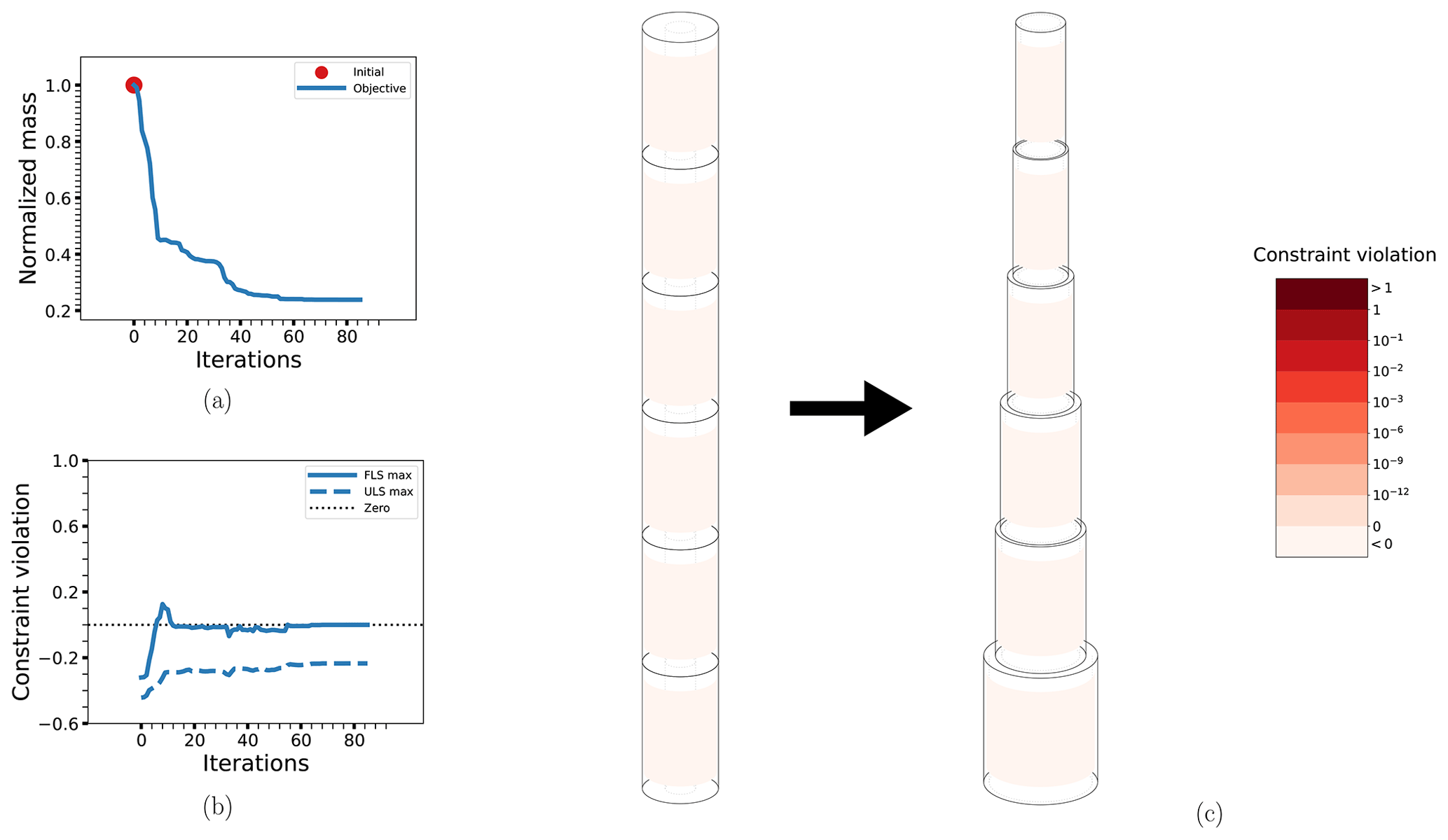
Figure 9The optimization process for case BEAM-DA: the objective function (a), maximum non-linear constraint violations (b) and the change in the design from initial to final configuration (c). Details as in previous figures.
4.2 OC3 Monopile
Beginning with the two basic cases for the OC3 Monopile, OC3-PA and OC3-DA, displayed in Figs. 10 and 11, respectively, we see that the behavior is fairly similar to the Simple Beam cases without connected design variables. Despite having more than twice the number of design variables, convergence is achieved in about the same number of iterations. The main new detail in the solution is that the second element from the bottom does not follow the otherwise apparent pattern of monotonically increasing diameters from top to bottom. In fact, this element has a smaller diameter than the element above, with a comparatively increased thickness to compensate. This is expected to be due to the wave loads, which are driven more by the diameter. The reason this does not happen for the Simple Beam cases is most likely because the smaller number of elements cannot resolve this effect. Otherwise, there is in the probabilistic case a much larger constraint violation at some intermediate points and the objective function initially increases above its starting value, but this does not seem to have much of an effect on the overall solution. More detailed results are shown in Table 7.
Table 7Selected summary results of cases OC3-PA and OC3-DA. Design variable numbers run from 1 (bottom element) to 14 (top element).

Figure 10The optimization process for case OC3-PA: the objective function (a), maximum non-linear constraint violations (b) and the change in the design from initial to final configuration (c). Details as in previous figures.
Figure 11The optimization process for case OC3-DA: the objective function (a), maximum non-linear constraint violations (b) and the change in the design from initial to final configuration (c). Details as in previous figures.
Next, the effect of including D−t ratio constraints for all elements is shown in the results from case OC3-PA-DT in Fig. 12. With this constraint in place, the low-thickness, high-diameter solution obtained previously is no longer feasible and the result is a solution which balances the reduction more evenly among the thicknesses and diameters. The result is in a sense more pleasing from a practical point of view, since it is more in line with a design that would actually be manufactured; both due to the lack of very large diameters and because one avoids the wave-load-induced “hourglass shape” seen in the previous two cases. The convergence is also faster (73 vs. 140 iterations), though there is one additional (very short) outer iteration required. On the other hand, the D−t ratio constraint is a lot more strict overall and less than 10 % reduction in mass is possible. In fact, the initial OC3 design is not feasible with respect to this constraint, which is why the objective function is increased by quite some amount at the beginning of the first loop. Note also that, as opposed to other comparable cases, the final design is softer (at 0.24 Hz) than the initial design (at 0.28 Hz).

Figure 12The optimization process for case OC3-PA-DT: the objective function (a), maximum non-linear constraint violations (b) and the change in the design from initial to final configuration (c). Details as in previous figures.
Randomizing the initial OC3 design gives the results displayed for OC3-PA-RND in Fig. 13. This initial design is both heavier and much less feasible (a probability of failure of 1 essentially in several locations) than the initial OC3 design, which seems to make the convergence a bit slower in this case but not by too much. The solution is not exactly the same as for OC3-PA, but the difference is negligible (1 % or less in the design variables and less than 0.005 % in the objective). This is within the expected variation caused by the small inherent randomness in the surrogate modeling.
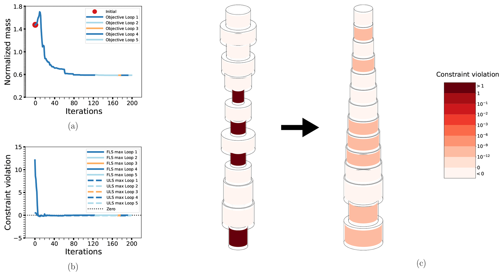
Figure 13The optimization process for case OC3-PA-RND: the objective function (a), maximum non-linear constraint violations (b) and the change in the design from initial to final configuration (c). Details as in previous figures.
Finally, the effects of no wave loads (OC3-PA-NW), only fatigue constraints (OC3-PF) and only extreme load constraints (OC3-PU) are shown in the results in Figs. 14, 15 and 16, respectively. As would be expected, the removal of the wave loads leads to a slightly lighter design and one where the element diameters consistently decrease from bottom to top. The difference in convergence behavior is likely negligible and mostly due to the randomness in the surrogate modeling. The resulting design has a slightly higher utilization of extreme loads. Since the fatigue constraints generally dominate over the extreme load constraints, the results for OC3-PF are as expected, with negligible differences in the final solution compared with OC3-PA and OC3-PA-RND. Conversely, using only extreme load constraints as in OC3-PU results in a final design that has about 16 % less mass than OC3-PA. This case also removes the visible effect of the wave loads on the solution, most likely because (at least for this loading scenario) the extreme loads caused by the waves are much less significant than the corresponding fatigue loads. Otherwise, the behavior is more or less as in the other cases.
More detailed results for OC3-PA-DT, OC3-PA-RND, OC3-PA-NW, OC3-PF and OC3-PU can be found in Table 8.
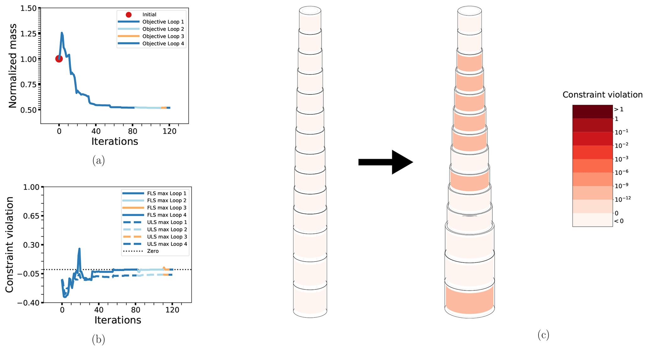
Figure 14The optimization process for case OC3-PA-NW: the objective function (a), maximum non-linear constraint violations (b) and the change in the design from initial to final configuration (c). Details as in previous figures.
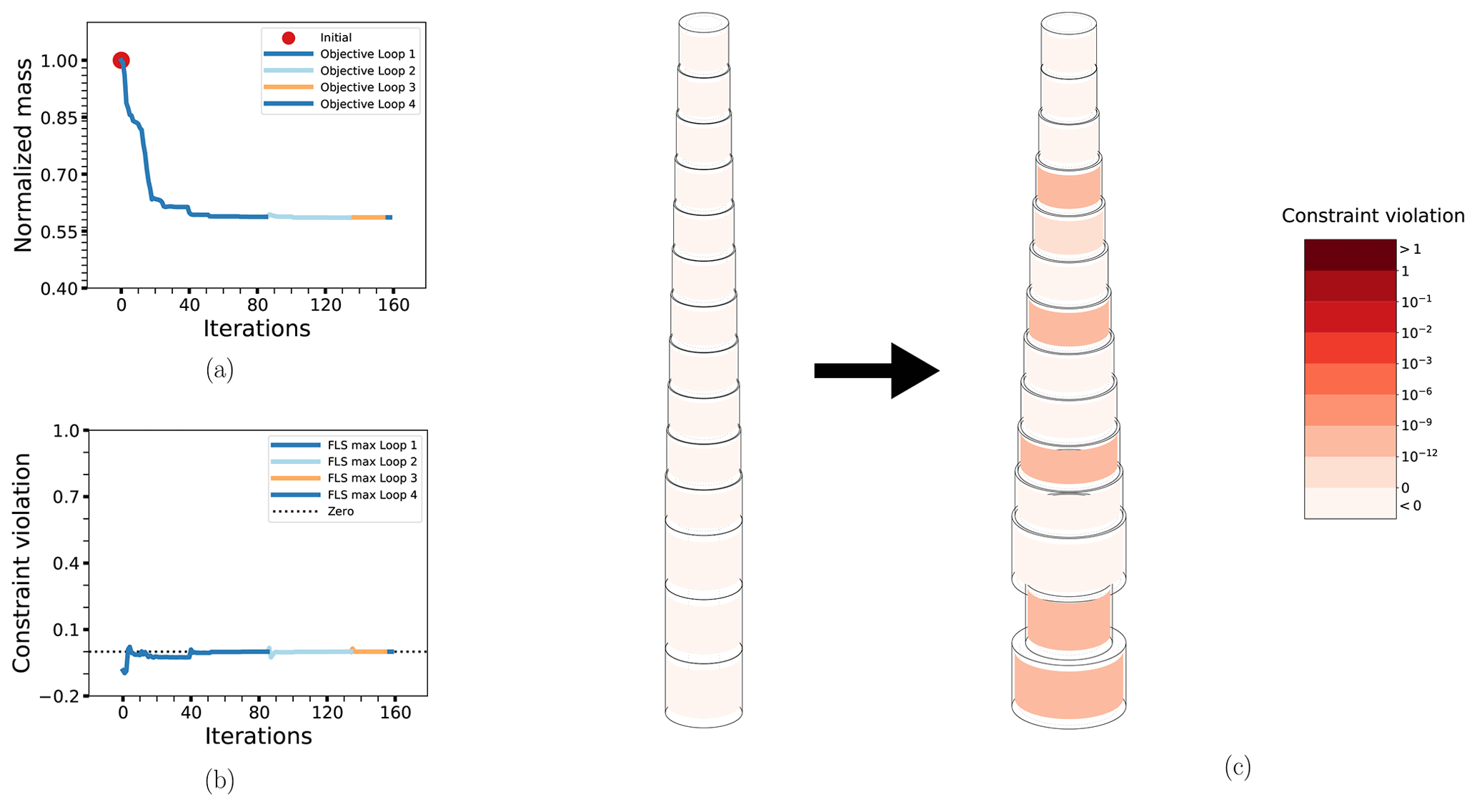
Figure 15The optimization process for case OC3-PF: the objective function (a), maximum non-linear constraint violations (b) and the change in the design from initial to final configuration (c). Details as in previous figures.

Figure 16The optimization process for case OC3-PU: the objective function (a), maximum non-linear constraint violations (b) and the change in the design from initial to final configuration (c). Details as in previous figures.
Table 8Selected summary results of cases OC3-PA-DT, OC3-PA-RND, OC3-PA-NW, OC3-PF and OC3-PU. Design variable numbers run from 1 (bottom element) to 14 (top element).
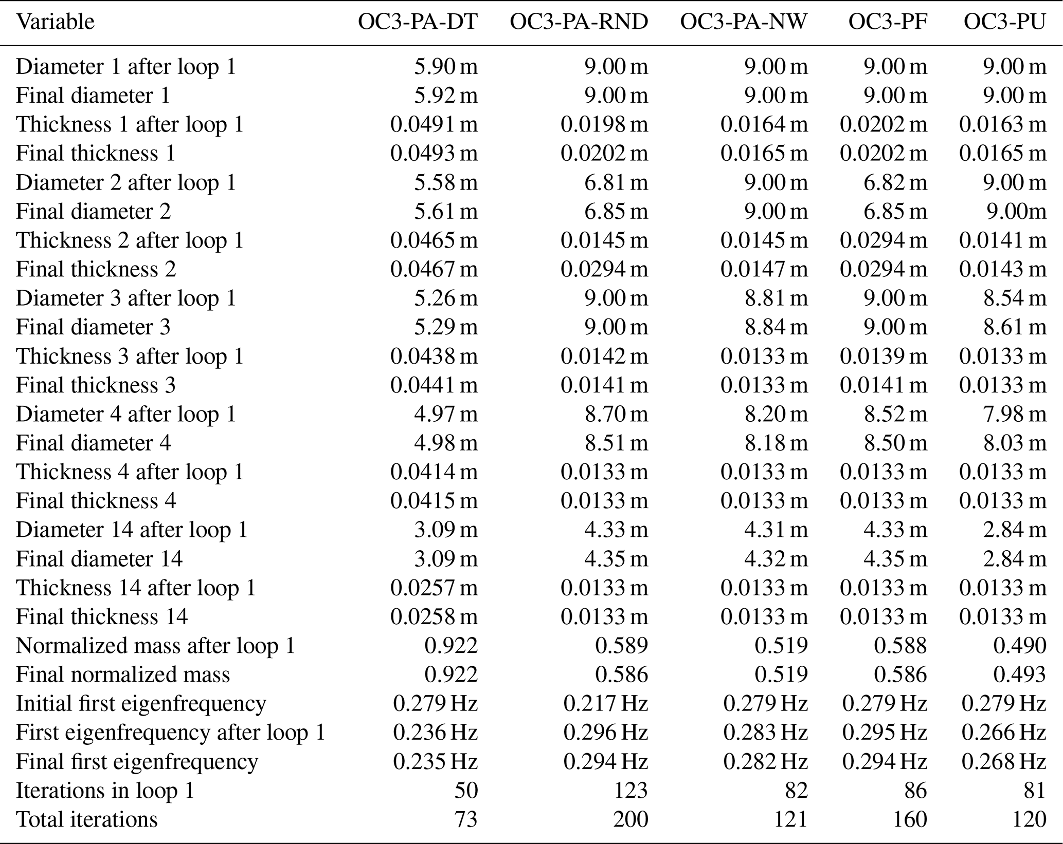
The results demonstrate quite clearly the capability of the proposed methodology to obtain reliable optimal support structure designs without making the optimization process itself much more computationally complex than in the deterministic case. In fact, the initial outer iteration of the RBDO approach requires about the same number of iterations as the corresponding deterministic optimization cases. The small amount of changes to the design that occur in the additional outer iterations indicate that, even with the simplifications involved in the response factorization, the surrogate model is a fairly accurate global approximation. Final convergence of the outer loop is then mostly necessary for convergence in a mathematical sense, and the added computational effort required is of lesser practical importance. Tightening the non-linear constraints slightly would ensure that feasible solutions were obtained after only one round of RBDO. The 50 samples used to train the surrogate model for the initial RBDO loop represent a very small additional computational effort compared to what is required for the optimization in general. Since the minimum number of function evaluations (and thus simulations) required for a single iteration is one base evaluation plus one additional evaluation for every design variable, 50 simulations becomes rather negligible (for the OC3 Monopile models, this number is surpassed after only two iterations). Even when using all 500 samples, the added computational effort is not particularly large when compared with a full optimization procedure (it is equivalent to at most 18 iterations of OC3 Monopile models or at most 46 iterations of unconnected Simple Beam models). All in all, this makes the proposed RBDO framework a realistic option if gradient-based deterministic optimization is computationally feasible for the desired application. We note that the computation time on a single workstation (16 cores at 2.7 GHz; 128 GB RAM) for one full evaluation of the constraints (including all simulations required for four loading scenarios and the computation of all design sensitivities) was about 40 s for the non-connected Simple Beam designs and about 100 s for the OC3 designs. The total solution time was consequently on the order of hours: at most 10–12 h for all outer iterations to complete but generally only a few hours for the initial outer iteration.
5.1 Obtained designs
The results obtained from RBDO do not appear functionally or systematically different than those obtained with deterministic optimization, producing designs that are similar and only slightly heavier. Note, for example, the large differences in maximum probability of failure compared to the small differences in total mass. The designs are driven by fatigue on the load side and the element thicknesses on the structural side, leading in general to designs with small thicknesses and large diameters. The OC3 Monopile designs tend to be quite a bit stiffer than the initial design, except when the loads or constraints are relaxed enough to allow for very light designs (as in the case of OC3-PA-NW and OC3-PU). The overall exception to these trends is the case with a D−t ratio constraint, though the thickness is also driving in this case. However, since the thickness cannot be arbitrarily smaller than the diameters in this case, the result is an effective upper bound on the thickness corresponding to the values where the overall design (with much smaller diameters than the other cases) is at the boundary imposed by the non-linear constraints. All in all, this is beneficial for the design process, since reliability-based constraints do not seem to change anything fundamental about the problem or introduce anything phenomenologically new from the design point of view. By and large, this indicates that as long as the structural and load models can be successfully adapted to the probabilistic setting, e.g., in the manner done in this study, then most if not all of previous knowledge and experience from deterministic design optimization is still valid and useful. On the other hand, this should not be taken to mean that probabilistic constraints can be easily replaced by more conservative deterministic ones. There is no way to determine sensible limits for such constraints – sensible here in the sense of being sufficiently safe while not being overly conservative – without performing some kind of non-deterministic analysis. Such analyses, for example, probabilistically tuned partial safety factors as basis for deterministically constrained optimization, are not necessarily more efficient than the present RBDO framework and cannot account for any potentially design-dependent changes that would be naturally accounted for with our methodology.
5.2 Simplifications
Some further simplifications have been made in the present analysis compared with more realistic applications. The main examples are the system model (with no soil model or detailed hydrodynamic modeling), the load analysis (simplified wave modeling, small number of environmental states considered) and the uncertainty modeling (potentially a much larger set of uncertainties might have been considered and a more detailed approach could have been used to obtain the specific uncertainty models). None of these simplifications are negligible but are not expected to affect the viability of the results dramatically either. The system and load modeling are not necessarily so far away from approaches commonly used for industrial applications, nor do they affect the system response in a way that would cause large deviations from the behavior seen in this study. The simplified (or lack of) soil structure interaction and hydrodynamic properties mostly serve to increase the global stiffness, reduce global damping and change the self weight of the system. These are systematic effects that may change the amplitudes of the response but are not expected to change the relative response to specific scenarios and so change, e.g., the complexity required to fit the surrogate model with respect to design changes. Similarly, the simplified load analysis is also not expected to affect the relative responses very much, especially for the fatigue analysis, where recent studies have shown that the distribution of fatigue damage over a comprehensive set of environmental states does not change drastically when the design changes, particularly as long as the eigenfrequency does not change too much (Stieng and Muskulus, 2018, 2019). Finally, the uncertainty analysis is mostly consistent with previous work in terms of the specific modeling but uses a smaller number of uncertainties than has typically been part of reliability studies. This can be seen as somewhat limiting in regards to the above points about the lack of added computational complexity, but it should be noted that it is usually possible to reduce the number of uncertainties down to a level closer to that of the present study by careful preliminary studies of the sensitivity to each uncertain parameter and subsequent elimination of all but the most important parameters. The automatic relevance determination of the GPR approach used presently is also advantageous for such a purpose.
In this work, we have presented a general methodology for performing RBDO of OWT support structures. The fundamental idea is that if the stochastic system response can be factorized into a design-dependent, deterministic (mean) response and a design-independent, probabilistic response, then it becomes possible to implement state-of-the-art RBDO, including state-of-the-art support structure design optimization methods, without adding much computational effort compared to deterministic optimization. The further advantages of the approach are that no assumptions about the functional representation of the probabilistic response are necessary, and since all design dependence is found in the deterministic part of the response, high-fidelity surrogate models can be fit for the probabilistic response while simultaneously making use of analytical methods for the estimation of design sensitivities. Together, this makes it possible to utilize recently developed gradient-based methods without having to make further adaptations of more general RBDO methods.
For the range of considered cases, the results show the feasibility of the proposed methodology. Although the overall approach includes an additional outer loop to ensure local fidelity of the surrogate model at the solution, these additional iterations are only necessary to ensure convergence in a stricter sense. For practical purposes, a single surrogate model fit and a single RBDO procedure suffices. Furthermore, the number of iterations of the RBDO procedure (not counting the solution of each reliability subproblem, which is computationally negligible when using a surrogate model), and hence the number of simulations required during optimization, is very close to that of the equivalent deterministic cases. The only additional computational effort is then found in the training of the surrogate model. However, this effort is comparable to that of a small number of additional iterations of the design optimization, especially for a larger number of design variables. Hence, the overall added computational complexity is small and makes the RBDO problem comparable to the equivalent deterministic optimization problem. The results also indicate that the RBDO framework does not change anything significantly about the kind of optimal designs that are obtained, as compared with deterministic design optimization. The same properties (fatigue and element thickness) seem to drive the designs, and the main differences are that probabilistically constrained designs are more conservative than their deterministic counterparts, as one would expect.
The current study is somewhat preliminary, in the sense that only a limited number of loading scenarios and constraints are considered, as well as the fact that the structural and environmental models are simplified and that limited effort has been put into refining, or otherwise optimizing, the methods used in the implementation of the overall framework. With regards to the simplifications, this is not expected to be a very limiting factor, though future work with higher fidelity is needed to ensure the practical viability of the proposed approach. As for the lack of refinement, this would indicate at least some potential for improving the methodology presented herein, which already works fairly well. It is likely that at the very least a more efficient design of experiment will be crucial if a larger amount of loading scenarios and higher-fidelity system modeling is to be made practical. Considering that many of the underlying optimization procedures used were originally developed for jacket support structures, it is expected that the current results, derived for monopiles, should be applicable with only minor modifications. Since very few studies of RBDO for OWTs have been done so far, in particular for support structure design, the current developments will hopefully open up new avenues for further research.
The data used for creating the figures and tables displaying the results are available in the Supplement. The code used to generate the results is very comprehensive and is, in its current form, not suitable for publication.
The supplement related to this article is available online at: https://doi.org/10.5194/wes-5-171-2020-supplement.
LESS formulated the main idea and implemented the method, conducted the analysis, created the figures and wrote the manuscript. MM provided essential input and suggestions throughout the process, aided in the formulation of the scope of the work and helped with the composition of the manuscript.
The authors declare that they have no conflict of interest.
This work has been partly supported by NOWITECH FME (Research Council of Norway, contract no. 193823) and by the Danish Council for Strategic Research through the project “Advancing BeYond Shallow waterS (ABYSS) – Optimal design of offshore wind turbine support structures”.
This research has been supported by the Norges Forskningsråd (grant no. 193823) and the Strategiske Forskningsråd (grant no. 1305-00020B).
This paper was edited by Athanasios Kolios and reviewed by two anonymous referees.
Abdallah, I., Lataniotis, C., and Sudret, B.: Parametric hierarchical kriging for multi-fidelity aero-servo-elastic simulators – Application to extreme loads on wind turbines, Probabilist. Eng. Mech., 55, 67–77, 2019. a
Andersen, L., Vahdatirad, M., Sichani, M., and Sørensen, J.: Natural frequencies of wind turbines on monopile foundations in clayey soils – A probabilistic approach, Comput. Geotech., 43, 1–11, 2012. a
Aoues, Y. and Chateauneuf, A.: Benchmark study of numerical methods for reliability-based design optimization, Struct. Multidiscip. O., 41, 277–294, 2010. a
Ben-Tal, A., Ghaoui, L. E., and Nemirovski, A.: Robust Optimization, Princeton University Press, New Jersey, USA, 2009. a
Brochu, E., Cora, V. M., and de Freitas, N.: A Tutorial on Bayesian Optimization of Expensive Cost Functions, with Application to Active User Modeling and Hierarchical Reinforcement Learning, available at: https://arxiv.org/abs/1012.2599 (last access: 18 July 2019), 2010. a
Caboni, M., Minisci, E., and Riccardi, A.: Aerodynamic Design Optimization of Wind Turbine Airfoils under Aleatory and Epistemic Uncertainty, J. Phys. Conf. Ser., 1037, 042011, https://doi.org/10.1088/1742-6596/1037/4/042011, 2018. a
Carswell, W., Arwade, S. R., DeGroot, D. J., and Lackner, M. A.: Soil–structure reliability of offshore wind turbine monopile foundations, Wind Energy, 18, 483–498, 2015. a
Chen, C. and Duffour, P.: Modelling damping sources in monopile‐supported offshore wind turbines, Wind Energy, 21, 1121–1140, 2018. a
Chen, X., Hasselman, T., and Neill, D.: Reliability based structural design optimization for practical applications, in: Proceedings of the 38th AIAA structures, structural dynamics, and materials conference, AIAA, Florida, USA, 1997. a
Chew, K.-H., Tai, K., Ng, E. Y. K., and Muskulus, M.: Analytical gradient-based optimization of offshore wind turbine substructures under fatigue and extreme loads, Mar. Struct., 47, 23–41, 2016. a, b, c, d
Choi, S.-K., Grandhi, R. V., and Canfield, R. A.: Reliability-based Structural Design, Springer-Verlag, London, UK, 2007. a, b
Couceiro, I., París, J., Navarrina, F., Guizán, R., and Colominas, I.: Optimization of Offshore Steel Jackets: Review and Proposal of a New Formulation for Time-Dependent Constraints, Arch. Comput. Method. E., https://doi.org/10.1007/s11831-019-09342-y, online first, 2019. a, b
Damgaard, M., Andersen, L., Ibsen, L., Toft, H., and Sørensen, J.: A probabilistic analysis of the dynamic response of monopile foundations: Soil variability and its consequences, Probabilist. Eng. Mech., 41, 46–59, 2015. a, b
Depina, I., Le, T. M. H., Fenton, G., and Eiksund, G.: Reliability analysis with Metamodel Line Sampling, Struct. Saf., 60, 1–15, 2016. a
Depina, I., Papaioannou, I., Straub, D., and Eiksund, G.: Coupling the cross-entropy with the line sampling method for risk-based design optimization, Struct. Multidiscip. O., 55, 1589–1612, 2017. a
Det Norske Veritas: Design of Offshore Wind Turbine Structures, Offshore Standard, DNV-OS-J101, DNV-GL, Høvik, Norway, 2016. a, b
Dimitrov, N. K.: Structural Reliability of Wind Turbine Blades, PhD thesis, Technical University of Denmark, 2013. a
Dong, W., Moan, T., and Gao, Z.: Fatigue reliability analysis of the jacket support structure for offshore wind turbine considering the effect of corrosion and inspection, Reliability Engineering and System Safety, 106, 11–27, 2012. a
Du, X. and Chen, W.: Sequential Optimization and Reliability Assessment Method for Efficient Probabilistic Design, J. Mech. Design, 126, 225–233, 2004. a
Dubourg, V.: Adaptive surrogate models for reliability analysis and reliability-based design optimization, PhD thesis, Blaise Pascal University, Claremont-Ferrand, France, 2011. a
Enevoldsen, I. and Sørensen, J.: Reliability-based optimization in structural engineering, Struct. Saf., 15, 169–196, 1994. a, b
Fedem Technology: Fedem User's Guide, release 7.2.1, Fedem Technology AS, Trondheim, Norway, 2016. a
Fischer, T., de Vries, W., and Schmidt, B.: Upwind Design Basis, Technical Report, Endowed Chair of Wind Energy (SWE) at the Institute of Aircraft Design, Stuttgart University, 2010. a
Frangopol, D. M. and Maute, K.: Reliability-Based Optimization of Civil and Aerospace Structural Systems, in: Engineering Design Reliability Handbook, edited by: Nikolaidis, E., Ghiocel, D. M., and Singhal, S., CRC Press, Boca Raton, USA, 2005. a
Häfele, J., Gebhardt, C. G., and Rolfes, R.: A comparison study on jacket substructures for offshore wind turbines based on optimization, Wind Energ. Sci., 4, 23–40, https://doi.org/10.5194/wes-4-23-2019, 2019. a, b
Haj, A.-K. E., Soubra, A.-H., and Fajoui, J.: Probabilistic analysis of an offshore monopile foundation taking into account the soil spatial variability, Comput. Geotech., 106, 205–216, 2019. a
Hu, W.: Reliability-Based Design Optimization of Wind Turbine Systems, in: Advanced Wind Turbine Technology, edited by: Hu, W., Springer International Publishing AG, Cham, Switzerland, 2018. a, b
Hu, W., Choi, K. K., and Cho, H.: Reliability-based design optimization of wind turbine blades for fatigue life under dynamic wind load uncertainty, Struct. Multidiscip. O., 54, 953–970, 2016. a
Hübler, C. J.: Efficient probabilistic analysis of offshore wind turbines based on time-domain simulations, PhD thesis, Leibniz Universität Hannover, 2019. a
Huchet, Q., Mattrand, C., Beaurepaire, P., Relun, N., and Gayton, N.: AK-DA: An efficient method for the fatigue assessment of wind turbine structures, Wind Energy, 22, 638–652, 2019. a
International Electrotechnical Commission: Wind turbines – Part 3: Design requirements for offshore wind turbines, International Standard, IEC 61400-3, IEC, Geneva, Switzerland, 2009. a, b
Jiang, Z., Hu, W., Dong, W., Gao, Z., and Ren, Z.: Structural Reliability Analysis of Wind Turbines: A Review, Energies, 10, 2099, https://doi.org/10.3390/en10122099, 2017. a
Jin, R., Du, X., and Chen, W.: The use of metamodeling techniques for optimization under uncertainty, Struct. Multidiscip. O., 25, 99–116, 2003. a
Jones, D. R., Schonlau, M., and Welch, W. J.: Efficient Global Optimization of Expensive Black-Box Functions, J. Global Optim., 13, 455–492, 1998. a
Jonkman, J. and Musial, W.: Offshore Code Comparison Collaboration (OC3) for IEA Task 23 Offshore Wind Technology and Deployment, Technical Report, NREL/TP-5000-48191, NREL, Golden, USA, 2010. a, b
Jonkman, J., Butterfield, S., Musial, W., and Scott, G.: Definition of a 5-MW Reference Wind Turbine for Offshore System Development, Technical Report, NREL/TP-500-38060, NREL, Golden, USA, 2009. a
Kallehave, D., Byrne, B. W., Thilsted, C. L., and Mikkelsen, K. K.: Optimization of monopiles for offshore wind turbines, Philos. T. R. Soc. A, 373, 20140100, https://doi.org/10.1098/rsta.2014.0100, 2015. a
Kang, B.-S., Park, G.-J., and Arora, J. S.: A review of optimization of structures subjected to transient loads, Struct. Multidiscip. O., 31, 81–95, 2006. a
Karadeniz, H., Togan, V., Daloglu, A., and Vrouwenvelder, T.: Reliability-based optimisation of offshore jacket-type structures with an integrated-algorithms system, Ships Offshore Struc., 5, 67–74, 2010a. a
Karadeniz, H., Togan, V., and Vrouwenvelder, T.: Optimization of Steel Monopod-Offshore-Towers Under Probabilistic Constraints, Journal of Offshore Mechanics and Artcic Engineering, 132, 021605, https://doi.org/10.1115/1.4000401, 2010b. a
Kaymaz, I.: Application of kriging method to structural reliability problems, Struct. Saf., 27, 133–151, 2005. a
Kim, D. H. and Lee, S. G.: Reliability analysis of offshore wind turbine support structures under extreme ocean environmental loads, Renew. Energ., 79, 161–166, 2015. a
Kolios, A. I.: A Multi-Configuration Approach To Reliability Based Structural Integrity Assessment For Ultimate Strength, PhD thesis, Cranfield University, Cranfield, UK, 2010. a
Kostandyan, E. E. and Sørensen, J. D.: Reliability Assessment of Solder Joints in Power Electronic Modules by Crack Damage Model for Wind Turbine Applications, Energies, 4, 2236–2248, 2011. a
Kreisselmeier, G. and Steinhauser, R.: Systematic Control Design by Optimizing a Vector Performance Index, in: Proceedings of the IFAC Symposium on computer Aided Design of Control Systems, IFAC, Zurich, Switzerland, 1979. a, b
Kucherenko, S., Albrecht, D., and Saltelli, A.: Exploring multi-dimensional spaces: a Comparison of Latin Hypercube and Quasi Monte Carlo Sampling Techniques, available at: https://arxiv.org/abs/1505.02350 (last access: 18 July 2019), 2015. a
Lee, J.-O., Yang, Y.-S., and Ruy, W.-S.: A comparative study on reliability-index and target-performance-based probabilistic structural design optimization, Comput. Struct., 80, 257–269, 2002. a
Lee, Y.-S., Choi, B.-L., Lee, J. H., Kim, S. Y., and Han, S.: Reliability-based design optimization of monopile transition piece for offshore wind turbine system, Renew. Energ., 71, 729–741, 2014. a
Leimeister, M. and Kolios, A.: A review of reliability-based methods for risk analysis and their application in the offshore wind industry, Renew. Sust. Energ. Rev., 91, 1065–1076, 2018. a
Li, H., Cho, H., Sugiyama, H., Choi, K. K., and Gaul, N. J.: Reliability-based design optimization of wind turbine drivetrain with integrated multibody gear dynamics simulation considering wind load uncertainty, Struct. Multidiscip. O., 56, 183–201, 2017. a
Márquez-Domínguez, S. and Sørensen, J. D.: Fatigue Reliability and Calibration of Fatigue Design Factors for Offshore Wind Turbines, Energies, 5, 1816–1834, 2012. a, b
Marsland, S.: Machine Learning – An Algorithmic Perspective, 2nd Edn., CRC Press, Florida, USA, 2015. a
Melchers, R.: Structural reliability: analysis and prediction, Wiley, New York, USA, 1999. a
Mockus, J.: On the Bayes Methods for Seeking the Extremal Point, in: Proceedings of the 6th IFAC World Congress, IFAC, Boston, USA, 1975. a
Morató, A., Sriramula, S., and Krishnan, N.: Kriging models for aero-elastic simulations and reliability analysis of offshore wind turbine support structures, Ships Offshore Struc., 14, 545–558, 2019. a
Müller, K. and Cheng, P. W.: Application of a Monte Carlo procedure for probabilistic fatigue design of floating offshore wind turbines, Wind Energ. Sci., 3, 149–162, https://doi.org/10.5194/wes-3-149-2018, 2018. a
Negm, H. M. and Maalawi, K. Y.: Structural design optimization of wind turbine towers, Comput. Struct., 74, 649–666, 2000. a
Nocedal, J. and Wright, S. J.: Numerical Optimization, 2nd Edn., Springer, New York, 2006. a, b
Oest, J., Sørensen, R., Overgaard, L. C. T., and Lund, E.: Structural optimization with fatigue and ultimate limit constraints of jacket structures for large offshore wind turbines, Struct. Multidiscip. O., 55, 779–793, 2017. a, b
Oest, J., Sandal, K., Schafhirt, S., Stieng, L. E. S., and Muskulus, M.: On gradient-based optimization of jacket structures for offshore wind turbines, Wind Energy, 21, 953–967, 2018. a
Press, W. H., Teukolsky, S. A., Vetterling, W. T., and Flannery, B. P.: Numerical Recipes: The Art of Scientific Computing, 3rd Edn., Cambridge University Press, New York, 2007. a
Rafsanjani, H. M., Sørensen, J. D., Fæster, S., and Sturlason, A.: Fatigue Reliability Analysis of Wind Turbine Cast Components, Energies, 10, 466, https://doi.org/10.3390/en10040466, 2017. a
Rasmussen, C. E. and Williams, C. K. I.: Gaussian Processes for Machine Learning, MIT Press, Massachussets, USA, 2006. a, b
Ronold, K. O., Wedel-Heinen, J., and Christensen, C. J.: Reliability-based fatigue design of wind-turbine rotor blades, Eng. Struct., 21, 1101–1114, 1999. a
Rosenblatt, M.: Remarks on a Multivariate Transformation, Ann. Math. Stat., 23, 470–472, 1952. a
Rychlik, I.: A new definition of the rainflow cycle counting method, Int. J. Fatigue, 9, 119–121, 1987. a
Sandal, K., Verbart, A., and Stolpe, M.: Conceptual jacket design by structural optimization, Wind Energy, 21, 1423–1434, 2018. a
Santner, T. J., Williams, B. J., and Notz, W. I.: The Design and Analysis of Computer Experiments, 2nd Edn., Springer, New York, USA, 2018. a
Sørensen, J., Frandsen, S., and Tarp-Johansen, N.: Effective turbulence models and fatigue reliability in wind farms, Probabilist. Eng. Mech., 23, 531–538, 2008. a
Sørensen, J. D. and Tarp-Johansen, N. J.: Reliability-based Optimization and Optimal Reliability Level of Offshore Wind Turbines, Int. J. Offshore Polar, 15, 141–146, 2005. a, b
Sørensen, J. D. and Toft, H. S.: Probabilistic Design of Wind Turbines, Energies, 3, 241–257, 2010. a
Standards Norway: Design of steel structures, Rev. 3, February 2013, NORSOK Standard N-004, Standards Norway, Lysaker, Norway, 2013. a, b
Stieng, L. E. S. and Muskulus, M.: Reducing the number of load cases for fatigue damage assessment of offshore wind turbine support structures using a simple severity-based sampling method, Wind Energ. Sci., 3, 805–818, https://doi.org/10.5194/wes-3-805-2018, 2018. a, b
Stieng, L. E. S. and Muskulus, M.: Load case reduction for offshore wind turbine support structure fatigue assessment by importance sampling with two-stage filtering, Wind Energy, 22, 1472–1486, https://doi.org/10.1002/we.2382, 2019. a, b
Teixeira, R., O'Connor, A., Nogal, M., Nichols, J., and Spring, M.: Structural probabilistic assessment of Offshore Wind Turbine operation fatigue based on Kriging interpolation, in: Proceedings of 27th European Safety and Reliability Conference (ESREL 2017), 18–22, ESRA, Portoroz, Slovenia, 2017. a
Teixeira, R., Nogala, M., O'Connor, A., Nichols, J., and Dumas, A.: Stress-cycle fatigue design with Kriging applied to offshore wind turbines, Int. J. Fatigue, 125, 454–467, 2019. a
Thöns, S., Faber, M. H., and Rücker, W.: Support Structure Reliability Of Offshore Wind Turbines Utilizing An Adaptive Response Surface Method, in: Proceedings of the ASME 2010 29th International Conference on Ocean, Offshore and Arctic Engineering, 406–416, ASME, Shanghai, China, 2010. a, b
Toft, H. S. and Sørensen, J. D.: Reliability-based design of wind turbine blades, Struct. Saf., 33, 333–342, 2011. a, b
Toft, H. S., Svenningsen, L., Moser, W., Sørensen, J. D., and Thøgersen, M. L.: Assessment of wind turbine structural integrity using response surface methodology, Eng. Struct., 106, 471–483, 2016a. a
Toft, H. S., Svenningsen, L., Sørensen, J. D., Moser, W., and Thøgersen, M. L.: Uncertainty in wind climate parameters and their influence on wind turbine fatigue loads, Renew. Energ., 60, 352–361, 2016b. a, b
Tu, J., Choi, K. K., and Park, Y. H.: A New Study on Reliability-Based Design Optimization, J. Mech. Design, 121, 557–564, 1999. a
Tunga, M. A. and Demiralp, M.: A factorized high dimensional model representation on the nodes of a finite hyperprismatic regular grid, Appl. Math. Comput., 164, 865–883, 2005. a
Uys, P. E., Farkas, J., Jármai, K., and van Tonder, F.: Optimisation of a steel tower for a wind turbine structure, Eng. Struct., 29, 1337–1342, 2007. a
Valdebenito, M. A. and Schuëller, G. I.: A survey on approaches for reliability-based optimization, Struct. Multidiscip. O., 42, 645–663, 2010a. a
Valdebenito, M. A. and Schuëller, G. I.: A survey on approaches for reliability-based optimization, Struct. Multidiscip. O., 42, 645–663, 2010b. a
Velarde, J., Kramhøft, K., and Sørensen, J. D.: Reliability-based Design Optimization of Offshore Wind Turbine Concrete Structures, in: Proceedings of the 13th International Conference on Applications of Statistics and Probability in Civil Engineering, ICASP13, International Civil Engineering Risk and Reliability Association, Seoul, South Korea, 2019. a
Veldkamp, D.: A Probabilistic Evaluation of Wind Turbine Fatigue Design Rules, Wind Energy, 11, 655–672, 2008. a, b
Wandji, W. N., Natarajan, A., and Dimitrov, N.: Development and design of a semi-floater substructure for multi-megawatt wind turbines at 50+ m water depths, Ocean Eng., 125, 226–237, 2016. a
Wang, G. G. and Shan, S.: Review of Metamodeling Techniques in Support of Engineering Design Optimization, J. Mech. Design, 129, 370–380, 2006. a
Wei, K., Arwade, S. R., and Myers, A. T.: Incremental wind-wave analysis of the structural capacity of offshore wind turbine support structures under extreme loading, Eng. Struct., 79, 58–69, 2014. a
Yang, H. and Zhu, Y.: Robust design optimization of supporting structure of offshore wind turbine, J. Mar. Sci. Technol., 20, 689–702, 2015. a
Yang, H., Zhu, Y., Lu, Q., and Zhang, J.: Dynamic reliability based design optimization of the tripod sub-structure of offshore wind turbines, Renew. Energ., 78, 16–25, 2015. a
Yang, H., Zhang, X., and Xiao, F.: Dynamic Reliability based Design Optimization of Offshore Wind Turbines Considering Uncertainties, in: Proceedings of the Thirteenth (2018) Pacific-Asia Offshore Mechanics Symposium, 325–331, The International Society of Offshore and Polar Engineers, Jeju, South Korea, 2018. a
Yeter, B., Garbatov, Y., and Soares, C. G.: Reliability Of Offshore Wind Turbine Support Structures Subjected To Extreme Wave-Induced Loads And Defects, in: Proceedings of the ASME 2016 35th International Conference on Ocean, Offshore and Arctic Engineering, V003T02A060, ASME, Busan, South Korea, 2016. a, b
Yoon, G. L., Kim, S. B., and Kim, H. Y.: Reliability Analysis of Monopile for Offshore Wind Foundation Using the Response Surface Method, in: New Frontiers of Geotechnical Engineering GSP 423, 108–117, American Society of Civil Engineers, Shanghai, China, 2014. a
Yoshida, S.: Wind Turbine Tower Optimization Method Using a Genetic Algorithm, Wind Engineering, 30, 453–469, 2006. a
Youn, B. D. and Choi, K. K.: An Investigation of Nonlinearity of Reliability-Based Design Optimization Approaches, J. Mech. Design, 126, 403–411, 2003. a
Youn, B. D., Choi, K. K., and Park, Y. H.: Hybrid Analysis Method for Reliability-Based Design Optimization, J. Mech. Design, 125, 221–232, 2003. a, b
Zang, C., Friswell, M., and Mottershead, J.: A review of robust optimal design and its application in dynamics, Comput. Struct., 83, 315–326, 2005. a
Zwick, D., Muskulus, M., and Moe, G.: Iterative Optimization Approach for the Design of Full-Height Lattice Towers for Offshore Wind Turbines, Enrgy. Proced., 24, 297–304, 2012. a
The nominal expression for the Kreisselmeier–Steinhauser function does not actually include the global maximum as it does here, but for improved numerical performance it has been added (first term) and subtracted (exponential term) as suggested in the original study (Kreisselmeier and Steinhauser, 1979).