the Creative Commons Attribution 4.0 License.
the Creative Commons Attribution 4.0 License.
 | 03 Jan 2020
Cluster wakes impact on a far-distant offshore wind farm's power
Andreas Rott
Martin Dörenkämper
Gerald Steinfeld
Martin Kühn
Our aim with this paper was the analysis of the influence of offshore cluster wakes on the power of a far-distant wind farm. We measured cluster wakes with long-range Doppler light detection and ranging (lidar) and satellite synthetic aperture radar (SAR) in different atmospheric stabilities and analysed their impact on the 400 MW offshore wind farm Global Tech I in the German North Sea using supervisory control and data acquisition (SCADA) power data. Our results showed clear wind speed deficits that can be related to the wakes of wind farm clusters up to 55 km upstream in stable and weakly unstable stratified boundary layers resulting in a clear reduction in power production. We discussed the influence of cluster wakes on the power production of a far-distant wind farm, cluster wake characteristics and methods for cluster wake monitoring. In conclusion, we proved the existence of wake shadowing effects with resulting power losses up to 55 km downstream and encouraged further investigations on far-reaching wake shadowing effects for optimized areal planning and reduced uncertainties in offshore wind power resource assessment.
- Article
(9111 KB) - Full-text XML
- BibTeX
- EndNote


Wind energy utilization at sea is an increasingly important part for the transition of the mainly fossil-based energy system towards renewable electricity generation. By the end of 2018 offshore wind turbines with a capacity of 6382 MW were installed in German waters, 21 750 MW worldwide. A massive expansion of offshore wind energy utilization is expected in many countries. Germany alone aims at an installed capacity of 15 GW by the year 2030 (Mackensen, 2019). Most of this capacity will be installed in the North Sea and Baltic Sea mainly in large wind farm clusters. A wind farm cluster typically consists of several wind farms in the direct vicinity, often operated by different parties and featuring different wind turbine types and geometries. Here, we call a large accumulation of more than a hundred wind turbines a cluster.
Wind turbines extract energy from the atmosphere forming regions of reduced wind speed, so called wakes, behind them. Wakes of single wind turbines merge to a wind farm or cluster wake (e.g. Nygaard, 2014). We use the term cluster wake for the merged wakes of a large number of wind turbines of either the same or different type with no individual wind turbine wake identifiable anymore. Downstream turbines within a wind farm (e.g. Barthelmie and Jensen, 2010) and in neighbouring downstream clusters (e.g. Nygaard and Hansen, 2016) experience reduced wind speeds and reduced power generation caused by wake shadowing effects. With a rising offshore wind energy utilization, cluster wake shadowing effects will occur to an increasing degree, leading to power losses and uncertainties in offshore wind resource assessment.
Wind turbine wakes were subject of intensive research in the last decade. Wake measurements were mainly performed using the remote-sensing technique Doppler lidar (e.g. Aitken et al., 2014; Trabucchi et al., 2017; Bodini et al., 2017; Fuertes et al., 2018; Beck and Kühn, 2019), power analysis on the basis of SCADA data (e.g. Barthelmie and Jensen, 2010) or Doppler radar (e.g. Hirth et al., 2014). Furthermore, several numerical studies investigated wind turbine wakes using large eddy simulation (LES) (e.g. Churchfield et al., 2012; Abkar and Porté-Agel, 2015; Dörenkämper et al., 2015b; Lignarolo et al., 2016; Vollmer et al., 2016). In an unstable atmosphere, e.g. in cold air over warm water, vertical turbulence leads to a well mixed boundary layer and causes a faster wake recovery. In stable conditions, e.g. in warm air over cold water, wake deficits can last far downstream. Hansen et al. (2011), Dörenkämper et al. (2015b) and Lee et al. (2018) investigated wake recovery with respect to atmospheric stability and found an increased length of wakes in stable stratification. Optimized wind farm layouts on the basis of the prevailing wind rose and stability distribution to reduce wake effects are commonly used (e.g. Emeis, 2009; Turner et al., 2014; Schmidt and Stoevesandt, 2015).
Cluster wakes are recently coming into the scientific focus with an increased offshore wind energy utilization. Due to the large dimensions of cluster wakes experimental investigations have been made with measurement systems capable of covering large areas like satellite synthetic aperture radar (SAR) (e.g. Hasager et al., 2015), research aircraft (e.g. Platis et al., 2018) and Doppler radar (e.g. Nygaard and Newcombe, 2018). Numerical studies were carried out by implementing wind farms in mesoscale models (e.g. Fitch et al., 2012; Volker et al., 2015). Wakes of large offshore wind farm clusters over distances of more than 10 km were first observed using data from satellite SAR (Christiansen and Hasager, 2005). Li and Lehner (2013) and Hasager et al. (2015) analysed offshore wind farm wakes using SAR images and compared the long, visible wakes to results of mesoscale models. Nygaard and Hansen (2016) analysed the power production of an offshore wind farm before and after the commissioning of a wind farm located 3 km to the west on the basis of SCADA data and discovered power losses caused by wakes of the upstream wind farm in the first rows of the downstream wind farm. Nygaard and Newcombe (2018) used dual Doppler wind radar to measure the inflow and the wake of an offshore wind farm and found wind speed deficits up to the maximal achievable downstream distance of 17 km possible with the used setup. They analysed a case with steady wind direction and speed and observed the cluster wake for over 1 h; stability information was not available. Platis et al. (2018) used in situ measurements taken with a research aircraft at hub height behind offshore wind farm clusters in the German North Sea and identified wakes with lengths of up to 55 km under stable atmospheric conditions, up to 35 km in neutral conditions and up to 10 km in unstable conditions. Siedersleben et al. (2018b) used the same flight measurements as Platis et al. (2018) to evaluate a wind farm parametrization (Fitch et al., 2012) in the numerical Weather Research and Forecasting model (WRF) that is well established in wind energy applications (e.g. Pryor et al., 2018b; Witha et al., 2019; Dörenkämper et al., 2015a). Additionally they presented an analysis of aircraft wake measurements in five different heights 5 km downwind of the cluster. The wake deficit existed in all considered height levels, also 50 m above the upper tip height of the rotor. Siedersleben et al. (2018a) investigated the micro-meteorological consequences of cluster wakes due to mixing effects in the atmosphere using the flight measurements from Platis et al. (2018). Pryor et al. (2018a) evaluated the downstream impact of large onshore wind farms in North America using the wind farm parametrization by Fitch et al. (2012) in convection-permitting mesoscale WRF simulations. Lundquist et al. (2019) analysed the physical, economic and legal consequences of wake effects between large onshore wind farms with sizes of more than a hundred megawatt each.
Wind farm cluster wakes in the far field of more than 20 km downstream have not been measured over longer periods. Satellite SAR just offers the possibility to take snapshots of the wind field. Doppler radar has been deployed on the coast monitoring a nearshore wind farm (Nygaard and Newcombe, 2018) but not in an offshore wind farm to use the full measurement range for wake analysis. Doppler lidar, which successfully monitored wind turbine wakes, was considered not to be able to achieve the measurement range needed to investigate full cluster wakes. Furthermore, the influence of cluster wakes on the power production of far downstream wind farms has not been analysed. The influence of atmospheric stability on the development and recovery of cluster wakes has not been studied in detail.
The objective of this paper is to analyse whether offshore cluster wakes have a significant and continuous influence on the power generation of a far downstream wind farm and how this influence depends on atmospheric stability. For this purpose we investigated two exemplary cases of cluster wakes approaching the 400 MW wind farm Global Tech I in the North Sea during situations with different atmospheric stabilities by means of four synchronized data sets, namely
-
large-area satellite SAR wind data,
-
continuous platform-based long-range Doppler lidar wind monitoring,
-
operational data of the wind farm Global Tech I and
-
meteorological measurements for atmospheric stability characterization.
We follow Platis et al. (2018) in their definition of the cluster wake deficit as the difference in the wind speeds from the manually selected wake region and a neighbouring free-flow region since the inflow wind speed of the wake generating cluster as reference is typically not known. Furthermore, regional and temporal differences in the wind field distort a comparison of the far-distant points in front of and far behind a cluster. Therefore, the adjacent regions in and aside the wakes are compared. Wake and free-flow regions are identified manually in this analysis.
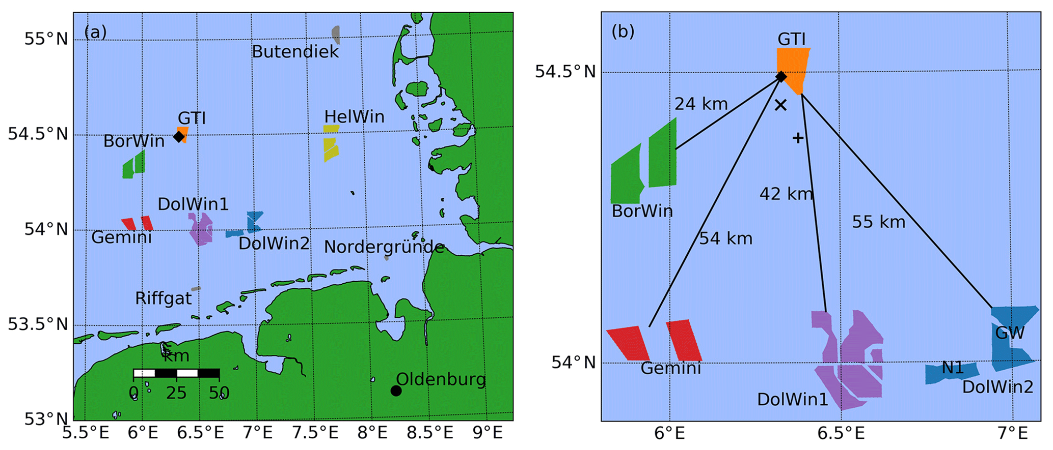
Figure 1(a) Overview of the considered area in the southern North Sea with wind farms and clusters shown. (b) Close view on GT I and neighbouring wind farm clusters. The position of the lidar in GT I on turbine GT58 (filled ⋄) and the offshore substation (OSS) “Hohe See” (×) and the transformer platform “BorWin gamma” (+) are marked; distances to upstream clusters are also shown. We measured wakes of all clusters in (b) and exemplary present the wakes of the BorWin and the DolWin2 clusters in this work. Information on the wind farms and full names are listed in Table 1.
The paper is structured as follows. Section 2 introduces the experimental setup in the North Sea; measurements taken with lidar, SAR and meteorological sensors; and data processing. Section 3 presents two exemplary cluster wake cases affecting the wind farm Global Tech I. In Sect. 4 we discuss the influence of cluster wakes on the power production of a far downstream wind farm as well as cluster wake characteristics and methods for cluster wake monitoring. Section 5 concludes on the findings and closes the paper.
In this study different data sources have been used: meteorological measurements, wind farm production data (supervisory control and data acquisition, SCADA) and remote-sensing data from a Doppler lidar (light detection and ranging) measurement campaign, and satellite SAR (synthetic aperture radar) data. A description of these data sources is given in this section. Our measurement campaign started in late July 2018 and was planned to last 1 year. The measurements we present in this paper were taken on 11 October 2018 and 6 February 2019. All measurement data in this study were recorded in Coordinated Universal Time (UTC).
2.1 Wind farms and SCADA data
As of early 2019, several offshore wind farms were installed mainly in clusters in the German and Dutch North Sea. Focus of this work is on the effects on the 400 MW wind farm Global Tech I (GT I), which is one of the world's most distant offshore wind farms with a coastal distance of more than 100 km. We analyse the impact of two large wind farm clusters, namely the 802 MW “BorWin” cluster located about 25 km southwest and the 914 MW “DolWin2” cluster 55 km southeast on the wind farm GT I.
Figure 1 gives an overview of the region around GT I while Fig. 2 displays its layout.
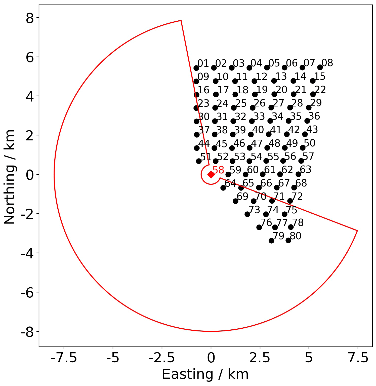
Figure 2Layout of the wind farm Global Tech I with turbine numbers. The turbine GT58, where we positioned the lidar, is marked in red (⋄). The achievable sector for lidar measurements is drawn.
Table 1Overview of offshore wind farms considered in this work (as of June 2019). The wind farms Borkum Riffgrund 2 (Orsted, 2018) and “Merkur Offshore” (Merkur Offshore, 2018) were in the commissioning phase and partly fed into the grid during our measurements; therefore, they are marked with smaller symbols in the relevant plots in this paper. D: rotor diameter, hH: hub height, Pr: rated power per turbine, No.: number of turbines per wind farm, ΣPr: rated power of wind farm. The numbers for the hub height are related to different reference levels, namely lowest astronomical tide (LAT), mean sea level (MSL) or just “over water”. These differences are not further considered here since the difference between LAT and MSL is typically around 2 m in the North Sea.

All coordinates in maps we show in the following, except Fig. 1, were transferred to the Gauss Krüger coordinate system and the origin was shifted to the lidar position at turbine GT58 in GT I (Fig. 2). Table 1 summarizes the main characteristics of the wind farms and clusters in the region. In the direct southwestern vicinity of GT I, the associated wind farms Hohe See and Albatros were under construction during the period of our measurement campaign with several transition pieces and a substation but no wind turbine towers installed. The first turbine was erected on 6 April 2019 (EnBW, 2019). The position of the Hohe See offshore substation (OSS) is marked in the following plots (×). The installation of the 900 MW high-voltage direct current (HVDC) platform BorWin gamma in the southeast corner of Hohe See was completed on 11 October 2018 (Petrofac, 2018); we also mark its position (+).
For the wind farm GT I, 10 min averaged SCADA data were available during the period of the measurements. Data of turbines in normal operation were considered; turbines with curtailed power below rated power were excluded from the analysis based on a SCADA status flag, a curtailment signal and consideration of pitch angles. For the wind farms BARD Offshore 1, Gode Wind 1+2 and Nordsee One we obtained hourly production data from Fraunhofer ISE (2019) and checked the operational status.
We analyse wind turbine power differences using the z score
with being the difference in the ith turbine's power Pi and the mean power of the turbines in the first row facing the wind direction (upstream turbines) normalized with the standard deviation of the power of the upstream turbines within the considered time span. Advection through the farm is not considered. We use the upstream turbines to calculate the z score instead of the turbines of the whole farm to avoid distortion by inner-farm wake effects.
2.2 Lidar measurements
We used a scanning long-range Doppler lidar system of type Leosphere Windcube 200S (serial no. WLS200S-024) in this study. The lidar system emits laser pulses into the atmosphere and analyses the light backscattered by aerosols for a Doppler shift proportional to the radial wind velocity in beam direction vr. The lidar is able to process wind speed information in >200 different ranges on the beam called range gates. For each range gate, the radial wind speed vr and the carrier-to-noise ratio (CNR) as a measure of the signal quality are stored. The lidar's scanner is able to point the beam in any desired direction in the hemisphere above and partly below the device.
We installed the lidar system on the transition piece (TP) of wind turbine GT58 in GT I (filled ⋄ in Figs. 1 and 2). The height of its scanner was approximately 24.6 m a.m.s.l. (above mean sea level), 67.0 m below hub height and 9.0 m below lower blade tip height of the turbine. Figure 3 displays a picture of the lidar installed in GT I.
Table 2Overview of the different settings for the lidar plan position indicator (PPI) scans. Both scenarios covered different sectors of 150∘ width. Range gates are listed as minimal range : spacing : maximal range. Range gates are also referred to as “measurement points” in the following.

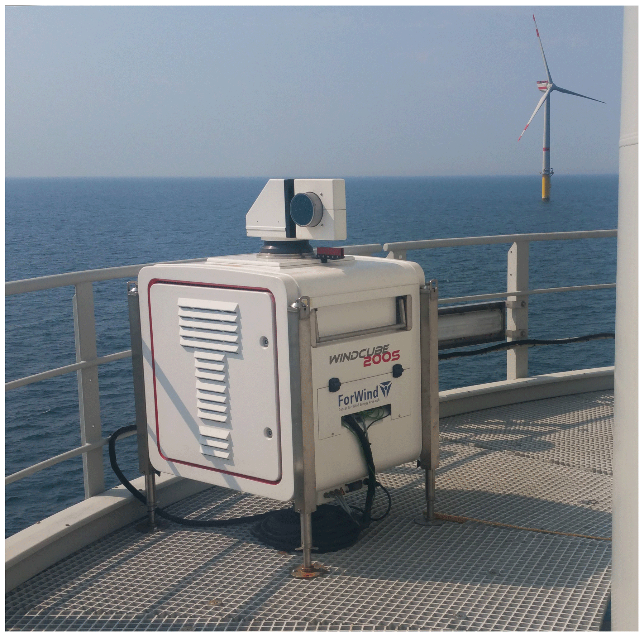
Figure 3Lidar system Windcube 200S on the transition piece of wind turbine GT58 in the offshore wind farm Global Tech I. On the right side of the image the tower of the turbine is visible while turbine GT51 northwest of GT58 can be seen in the background (cf. GT I layout in Fig. 2) (Stephan Voß, ForWind).
The lidar performed horizontal plan position indicator (PPI) scans (elevation angle φ was 0∘) with continuous scanner movement in different azimuthal sectors of 150∘ width upstream with two different settings, A and B, as listed in Table 2. We started with the slower scenario A aiming for a high measurement range. Later we optimized the measurements using scenario B, being 4 times faster and achieving similar ranges. In both scenarios the laser beam is scanned over an angle of 2∘ per measurement leading to spatial averaging perpendicular to the line of sight direction. After performing a scan, the lidar needs a few seconds to reset and start the next scan. Every few hours it performs a homing procedure of the scanner to assure precise orientation. The laser pulse length used in both scenarios was 400 ns, leading to a probe volume of approximately 70 m in the beam direction. The range gate spacing is listed in Table 2.
The offset in the azimuthal direction between geographic north and the lidar's north was corrected by scanning distant wind turbines in GT I with known positions (“hard targeting”). The resulting error in the azimuthal orientation Δφ was smaller than 0.1∘ and is therefore neglected.
The lidar was well aligned on the pitch and roll axis; errors were checked using the method of sea surface levelling (Rott et al., 2017). The resulting maximal error in the elevation Δϑ was less than 0.1∘. An additional error in the elevation angle of the lidar measurement occurs from a small movement of the TP due to the thrust on the rotor with a maximum of 0.1∘.
When regarding the height of the measurement locations, the curvature of the earth must be taken into account for the ranges achieved. The error introduced raises quadratically with range and reaches Δh8=5.02 m for a distance of 8 km and of Δh10=7.85 m for a distance of 10 km. The measurement errors we describe here can be neglected for the mainly qualitative analysis in this work.
2.3 Lidar data processing
Lidar scans were individually filtered on CNR minimal and maximal thresholds, a maximum range, and a minimal data density in the vr–CNR plane (similar to Beck and Kühn, 2017). For each PPI scan, the mean wind direction was determined by fitting a cosine function to all radial speeds vr of the scan over their azimuth angles φ. All vr were then transformed back to the absolute wind speed va in mean wind direction assuming the perpendicular wind component to vanish using
with φdiff being the difference angle between the beam direction and the mean wind direction. Sectors with measurement ranges almost perpendicular to the wind direction (∘) were excluded from the analysis because of an increasing error due to an overestimation of flow components perpendicular to the wind direction. We plot single lidar scans on their original polar grid. To obtain averaged lidar wind fields, we transferred the va-lidar data of each regarded scan to a Cartesian grid with a resolution of 50 m × 50 m, triangulating the data points and on each triangle performing linear barycentric interpolation to the grid points. We then calculated the cubic (or power) average on each grid point. Due to slightly changing wind directions in the averaging interval, points at the border of the scans were just included in the further analysis if no scan (scenario A) or less than 10 scans (scenario B) did not contribute at the grid point.
2.4 Atmospheric stability and meteorological data
Meteorological measurements of atmospheric stability are uncommon in offshore wind farms. Different methods for the derivation of stability exist (see Rodrigo et al., 2015 for an overview). We applied the bulk Richardson method from profile measurements according to Emeis (2018) based on the tropical observations of Grachev and Fairall (1997). We used the wind speed vTP, the temperature TTP on the height of the transition piece zTP, and the difference in the virtual potential temperatures at the height of the TP and at sea level, (see Appendix A), to derive the dimensionless bulk Richardson number
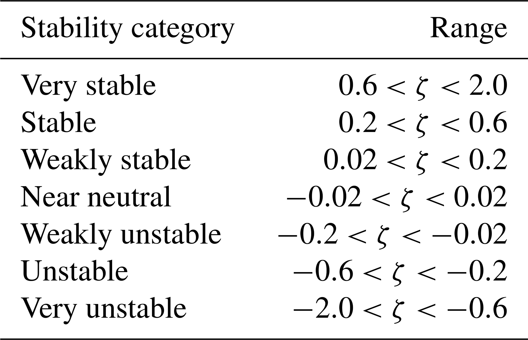
where g is the gravity acceleration. The dimensionless stability parameter,
and the stability classification in Table 3 were chosen for stability categorization.
Table 3Classification of atmospheric stability as suggested by Sorbjan and Grachev (2010).
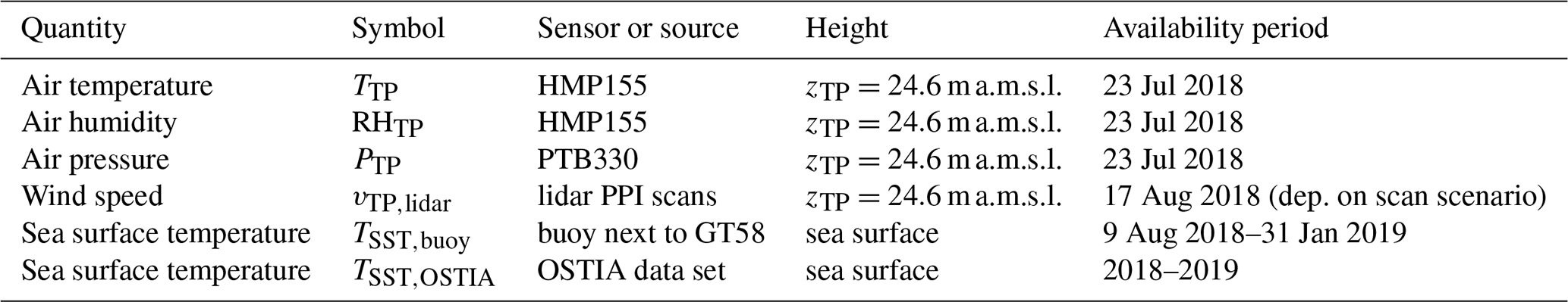
To be able to estimate ζ, we operated sensors for air pressure (Vaisala PTB330) as well as temperature and relative humidity (Vaisala HMP155) on the TP of turbine GT58. In one case (see Sect. 3.2.1) we used meteorological measurements from the nacelle of turbine GT58 provided by the wind farm operator as a second source of data to derive the stability parameter at height of the nacelle ζnac using the same methodology as described above. A buoy for the measurement of the sea surface temperature TSST was available from 9 August 2018 until 31 January 2019. We compared the measurements with the OSTIA data set (Donlon et al., 2012), both resampled to a 30 min interval (mean values for the buoy data, linear interpolation for the daily available OSTIA data set), and found a mean difference of 0.19 K. Since the buoy was not available during the whole lidar measurement campaign, we use TSST from the OSTIA data set to derive ζ. The wind speed on the height of the TP, vTP, for the purpose of atmospheric stability analysis was calculated from horizontal lidar PPI scans as described in Sect. 2.3 using data with a measurement range less than 3000 m. These measurements took place within the approaching cluster wakes, when present. This influences the calculation of the stability parameter but we see the wake as part of the inflow and do not try to correct for it. We averaged meteorological measurements to 30 min intervals. Table 4 shows an overview of the available meteorological data.
Table 4Overview of the available meteorological quantities to derive the stability parameter ζ. Availabilities disregard shorter data gaps. If no end time is stated, measurements are ongoing with date of 1 August 2019. Additional data from mesoscale simulations similar to the New European Wind Atlas (NEWA) data set were available but not listed in this table.
For a comparison of the potential power Ppot in the wind with the power harvested by free-flow turbines, we had to transfer wind speeds from measurement heights (zSAR=10 m, zTP=24.6 m) to hub height zhub=91.6 m. Following Emeis (2018), we used the logarithmic wind profile
with a correction function Ψm(z∕L) to account for the atmospheric stability to calculate the vertical wind profile. We used mesoscale data with a setup very similar to the production runs of the New European Wind Atlas (NEWA; see Witha et al., 2019; NEWA, 2019) internally deriving the roughness length z0 using Charnock's relation. We obtained the Obukhov length L from the stability parameter . The von Kármán constant reads as κ=0.4. The friction velocity u* was then calculated for the given pair of wind speed and height, e.g. zTP and uTP from Eq. (5). The wind speed on hub height was afterwards converted to the theoretical potential power Ppot using a power curve with the constant c derived from power data in the partial load range. We do not curtail Ppot at rated wind speeds allowing it to be larger than rated power.
2.5 SAR wind data
Satellite SAR remotely measures the roughness of the sea surface. Using a geophysical model to estimate wind direction, wind speeds over the ocean can be derived. In this work, we use publicly available already processed wind data from the Copernicus SAR satellite Sentinel-1A. The algorithm for wind field processing is described in Mouche (2011), an overview of its performance is given in ESA (2019) and the data product including quality flags is described in Vincent et al. (2019). Wind data at 10 m height are processed on a grid with a spatial resolution of 1 km×1 km. Wind speed estimates are in range from 0 to 25 m s−1 with a root mean square error (RMSE) smaller than 2.0 m s−1 and wind direction estimates have an RMSE below 30∘. The spatial coverage of the SAR images and the processed wind fields is 170 km × 80 km minimum with a revisit time of the order of days. A quality flag for the wind estimate (owiWindQuality, 0: high quality, 1: medium quality, 2: low quality, 3: bad quality; see Vincent et al., 2019) is provided within the data product. We use data with a quality flag ≤2. For the calculation of the potential power on hub height (see Sect. 2.4), we added constant wind speed values within the measurement accuracy to the SAR wind data to match the actual power production.
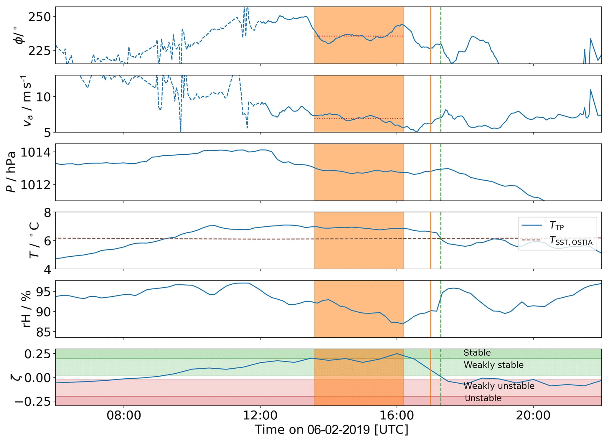
Figure 4Meteorological data at the lidar location on the height of the TP (24.6 m a.m.s.l.) of turbine GT58 on 6 February 2019. Top to bottom: wind direction ϕTP,lidar, wind speed vTP,lidar, air pressure PTP, air and sea surface temperature TTP and TSST,OSTIA, relative humidity RHTP, and the dimensionless stability parameter ζTP. Measurement times are marked as follows: vertical dashed line represents the SAR image (Fig. 5), vertical solid line represents the single lidar scan (Fig. 6), and shaded interval represents the averaged lidar wind field (Fig. 7). Mean wind speed and direction in the averaged lidar interval are marked by red horizontal dotted lines. Dashed lines in wind speed and direction indicate moist or foggy periods with reduced lidar data availability.
In this section we present an analysis of wake situations of the BorWin cluster on 6 February 2019 and of the DolWin2 cluster on 11 October 2018 based on Sentinel-1 SAR wind data, lidar measurements and SCADA power data of the wind farm GT I.
3.1 BorWin cluster wake on 6 February 2019
The BorWin cluster is located approximately 24 km upwind of GT I in southwesterly direction. We measured wakes from the cluster approaching GT I in stable stratified situations during our measurement campaign. Here we present a stably stratified situation in late winter 2018/2019 with low variation in the wind direction allowing us to analyse lidar scans of the same situation over a period of a couple of hours.
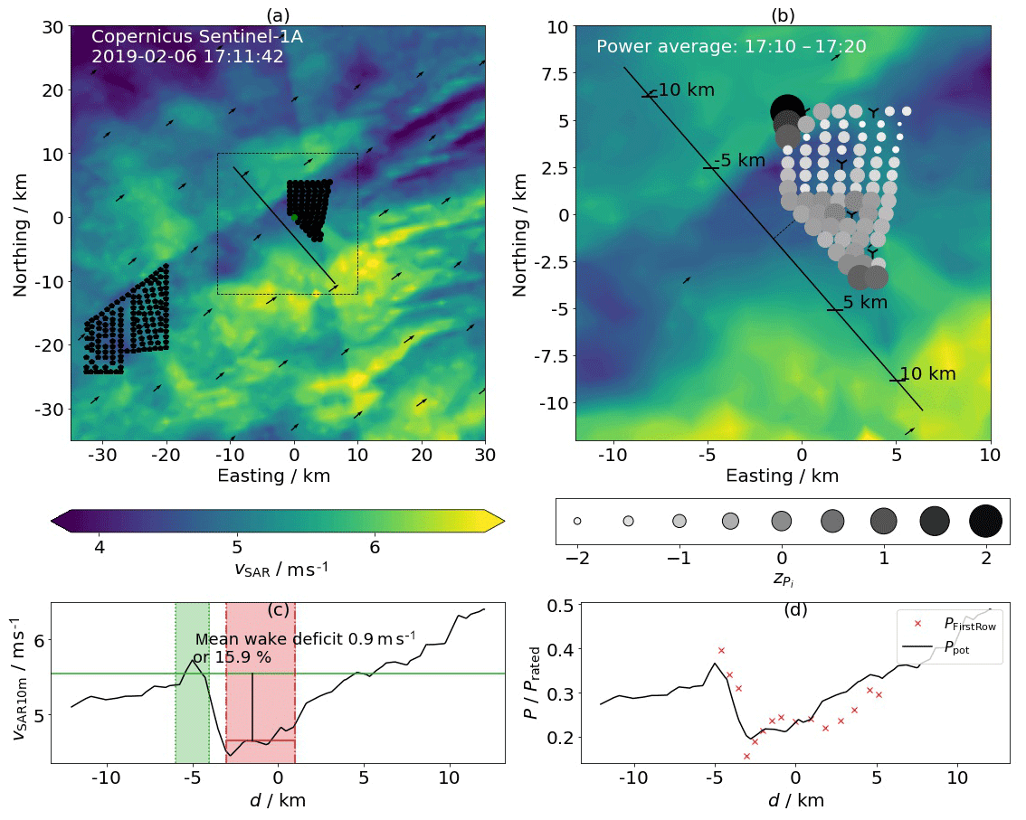
Figure 5Sentinel-1A Ocean Wind Field (Copernicus Sentinel data (2019)), measurement taken 6 February 2019 17:11:42 UTC. (a) Overview of the BorWin cluster and Global Tech I. (b) Close look on the BorWin wake hitting GT I. The solid line marks a virtual wake cut 2000 m upstream of turbine GT58 on which the wind field is evaluated. Marked distances correspond to the x axis of (c) and (d). The z score of the turbine power (see Eq. 1) is shown in greyscale for the relevant 10 min period (17:10–17:20 UTC); markers scale with z−zmin. Numbers of upstream turbines to calculate the z score are 1, 9, 16, 23, 30, 37, 44, 51, 58, 64, 69, 73, 76, 79, and 80. Turbines not operating the full period or operating at curtailed power are excluded and marked (Y-shaped marker). (c) Wind speeds along the wake cut from (b). Wake and the free stream are shaded (regions selected manually). (d) Potential power on hub height along the wake cut (solid line) together with the power produced by the upstream turbines in GT I within the regarded 10 min interval with turbine positions projected to the wake cut. A constant value of 1.0 m s−1 was added to vSAR,10 m for the calculation.
3.1.1 Meteorological conditions
In Fig. 4 we plot the measured wind speed and direction, air pressure, temperature and humidity, and the sea surface temperature from the OSTIA data set and the derived stability parameter ζ during 6 February 2019. On that day the frontal system of a cyclone southwest of Iceland crossed the German Bight. The warm front passed GT I in the morning, bringing air temperatures of about 6.9 ∘C in the warm sector over the 6.1 ∘C cold sea stabilizing the boundary layer. With decreasing humidity and disappearing fog, good lidar availability was achieved starting at approximately 10:00 UTC (short humid or foggy period of bad measurements around 12:00 UTC) with clear wakes of the BorWin cluster visible in the lidar scans. In the afternoon we choose a period with relatively constant wind direction from 13:35 to 16:12 UTC for analysing the averaged wake effects over a longer period of about 2.5 h. The period with stable stratification ended with the passage of the cold front at approximately 17:15 UTC.
3.1.2 SAR wind data
Figure 5 displays the analysis of a wind field derived from the measurement of the Copernicus satellite Sentinel-1A, which passed the German Bight at the end of the stable stratified period on 6 February 2019 as an overview of the wind field in the region around GT I. The wake of the BorWin cluster is clearly visible and extends approximately 24 km downstream until it partially hits the wind farm GT I. Further downstream of GT I an even higher wake deficit of the merged wakes of the BorWin cluster and GT I can be observed. The virtual wake cut (Fig. 5c) reveals a sharp transition from higher to lower wind speeds at the edge of the wake; a deficit in the SAR wind speed of 0.9 m s−1 is observed. Since the wake just partially hits GT I, it separates the farm into two regions: one in free flow and one affected by the wake. The turbines in free flow in the northwestern and southern corner of GT I produce significantly more power (>2σP) than the first upstream row of turbines produce on average (Fig. 5b). We confirm this result with the comparison of the 10 min power of the upstream-row turbines with the potential power on hub height derived from the inflow wind speed (Fig. 5d) which agrees well. Within the wake-affected region in GT I, typical inner-farm wake effects are visible through a power decrease in downstream direction (e.g. Barthelmie and Jensen, 2010, Fig. 5b) which are different in the northern and southern parts of the farm due to different turbine spacings in wind direction.
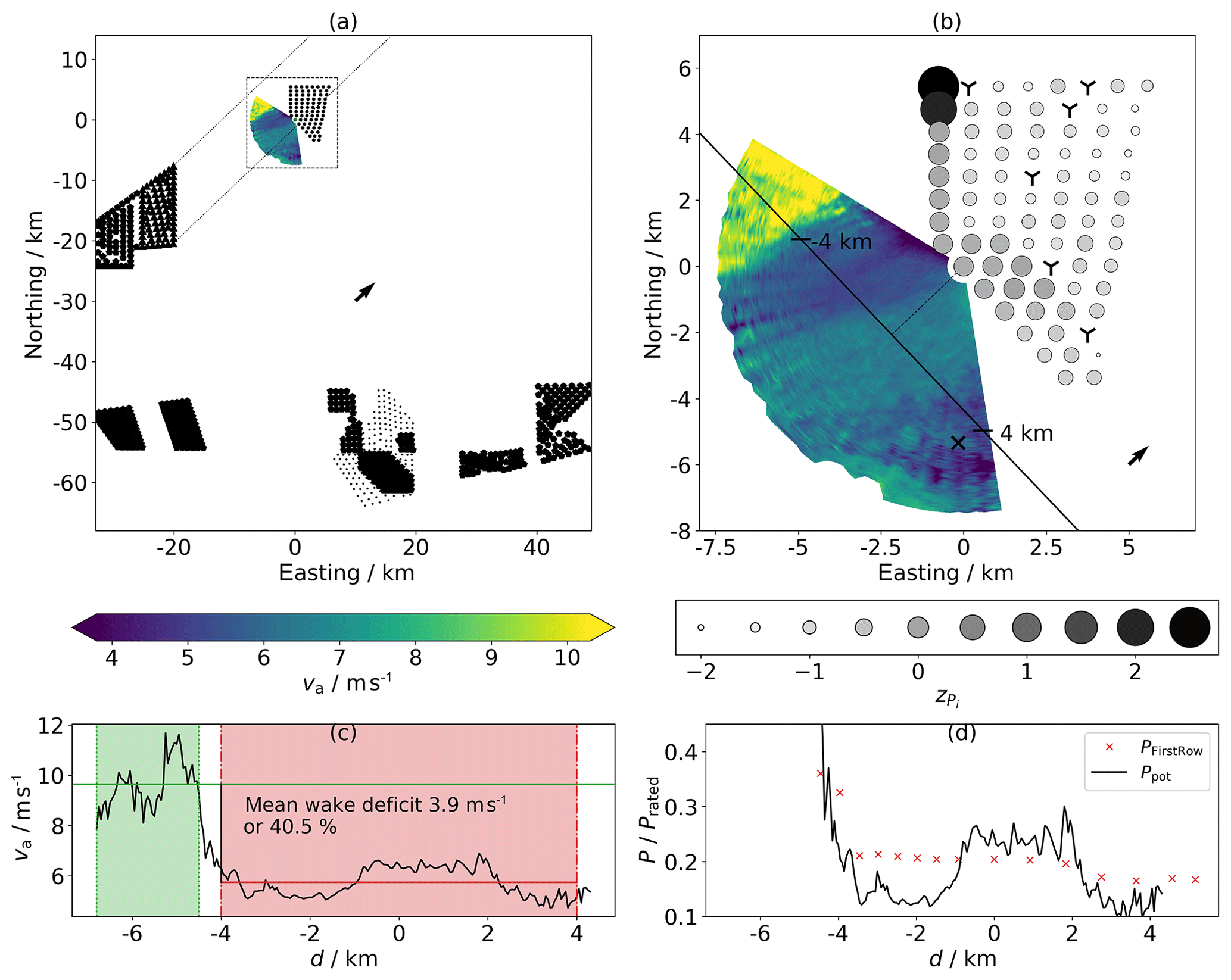
Figure 6Lidar scan (scenario B from Table 2) on 6 February 2019 16:58–17:01 UTC: (a) overview of the situation in the German Bight with lines parallel to the wind direction retrieved from the lidar scan from the corners of the upstream wind farm cluster BorWin. Lidar wind speed is colour coded (left colour bar). (b) Close view of the lidar wind field and the wind farm GT I. The z score of the not curtailed wind turbines' power in the current 10 min interval (16:50–17:00 UTC) is in greyscale (right colour bar), curtailed or non-operating turbines are marked (Y-shaped marker). Markers scale with z−zmin. Turbine numbers to calculate the z score as in Fig. 5. The substation Hohe See (×) is marked. The solid line marks a virtual wake cut 3000 m upstream of turbine GT58 on which the wind field is evaluated and drawn in (c). Areas of wake and free stream are shaded manually, the resulting wake deficit is stated. (d) Available power on hub height along the wake cut from (b) together with the power achieved from the upstream turbines in GT I with their positions projected to the wake cut.
3.1.3 Lidar wind fields
In Fig. 6 we present the analysis of a single lidar scan of the inflow of GT I. We observe a clear edge between high wind speeds in the undisturbed flow and lower wind speeds in the wake of the BorWin cluster, causing a clear separation of power production in the wind farm GT I in a free-flow and a wake region (Fig. 6b). The virtual wake cut in Fig. 6c illustrates the sharp transition region of just a few hundred metres width and highlights the wake deficit of 3.9 m s−1 or 40.5 %. The potential power on hub height derived from the inflow wind speed corresponds well with the power generated by the upstream row of turbines in the regarded 10 min interval (Fig. 6d). The two northerly upstream turbines are in the region of free flow and produce, with >2σP, significantly more power than the turbines being influenced by the BorWin wake.
In Fig. 7 we present an averaged lidar wind field calculated from 60 consecutive scans like the one in Fig. 6 in a period of approximately 157 min with relatively constant wind direction (see shaded areas in Fig. 4) to demonstrate the steadiness of the BorWin wake and its influence on power production. The wind speed along the virtual cut through the wind field in Fig. 7c reveals a strong average wake deficit of 2.3 m s−1, equivalent to 24.7 %. The transition region from wake flow to free flow is about 3 km wide resulting from the small changes in wind direction and thus the slightly different positions of the wake during the averaging time. Aside from the clear visible northerly edge of the BorWin wake, the southerly edge can be observed in the southerly corner of the lidar wind field and correspondingly in the wake cut (Fig. 7c). Wind speeds recover on both sides of the wake to similar values just above 9 m s−1. The average power of the GT I turbines reveals a clear reduction in the wake-affected region (Fig. 7b). The turbines in free flow produce (>2σP) above the average. Comparing the potential power on hub height along the wake cut together with the average power of the upstream-row turbines (Fig. 7d), we find a slight overestimation of the potential power in the wake region and an overestimated increase in the turbine power in the transition region. The position of the transition onset in the estimated power from the wind field and the measured power from the turbines agree well.
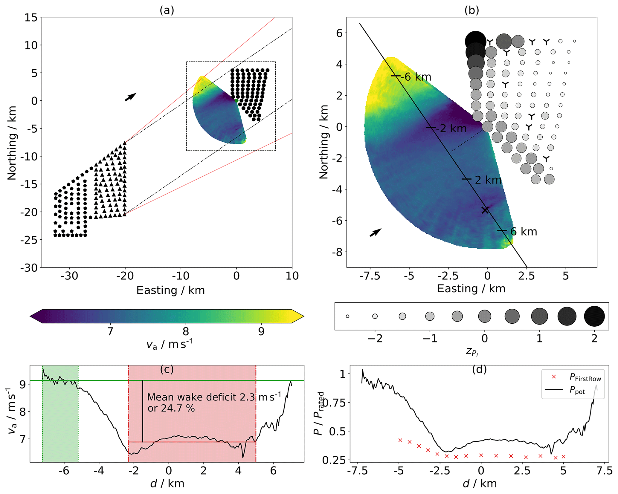
Figure 7As in Fig. 6 but averaged over 60 consecutive lidar scans (scenario B) corresponding to a period of 157 min (13:35–16:12 UTC); power data averaged over 170 min (13:30–16:20 UTC). Red lines in (a) indicate minimal and maximal wind directions within the averaging interval.
3.2 DolWin2 cluster wake on 11 October 2018
The DolWin2 cluster is approximately 55 km upstream of GT I in southeasterly direction. We regularly have indications in our measurements for wakes from the cluster approaching GT I in stably stratified situations. Here we present a situation in autumn 2018 with a change of stability over the course of the day. We present a single lidar scan and an averaged lidar wind field from a period with low variation in the wind direction in stable stratification. A complementary SAR scan from the morning of the day during weakly unstable stratification is available as well and analysed here.
3.2.1 Meteorological conditions
In Fig. 8 we plot the measured meteorological quantities on 11 October 2018. Since the lidar for measurements of wind speed and direction and the data of air temperature, pressure and humidity at TP height were not available during the whole day we added the mesoscale data from the New European Wind Atlas (NEWA) and measurements from the nacelle of turbine GT58 to the plots. A cyclone southwest of Iceland and a strong high-pressure area over Russia dominated the weather during the day. The North Sea was positioned in the warm sector of the cyclone between the cold front over the UK and the warm front spanning from Iceland to Norway. Southeasterly winds prevailed in the southern North Sea raising the air temperature in GT I between 12:00 and 14:00 UTC above the temperature of the still quite warm North Sea (approximately 16 ∘C) stabilizing the boundary layer. In the morning a shallow (weakly) unstable boundary layer of some hundred metres height occurred because the surface layer over land cooled down during the night to temperatures below sea surface temperature and moved with the prevailing flow over the sea. Aside from the stability obtained from NEWA (weakly unstable) and the nacelle measurements (unstable), this finding is further supported by temperature profiles sounded with radiosondes at the stations in Bergen (no. 10238) and Ekofisk (no. 1400) the same day. A weak inversion with temperatures of approximately 13.5 ∘C up to 300 m height appears in the profile at Bergen, 04:00 UTC, with a stronger temperature inversion above. At the Ekofisk site the temperature profile at 11:00 UTC shows a similar behaviour with the upper inversion being less pronounced and sunken to approximately 230 m height. This allows for dry adiabatic convection up to heights between 200 and 300 m for the prevailing sea surface temperature.
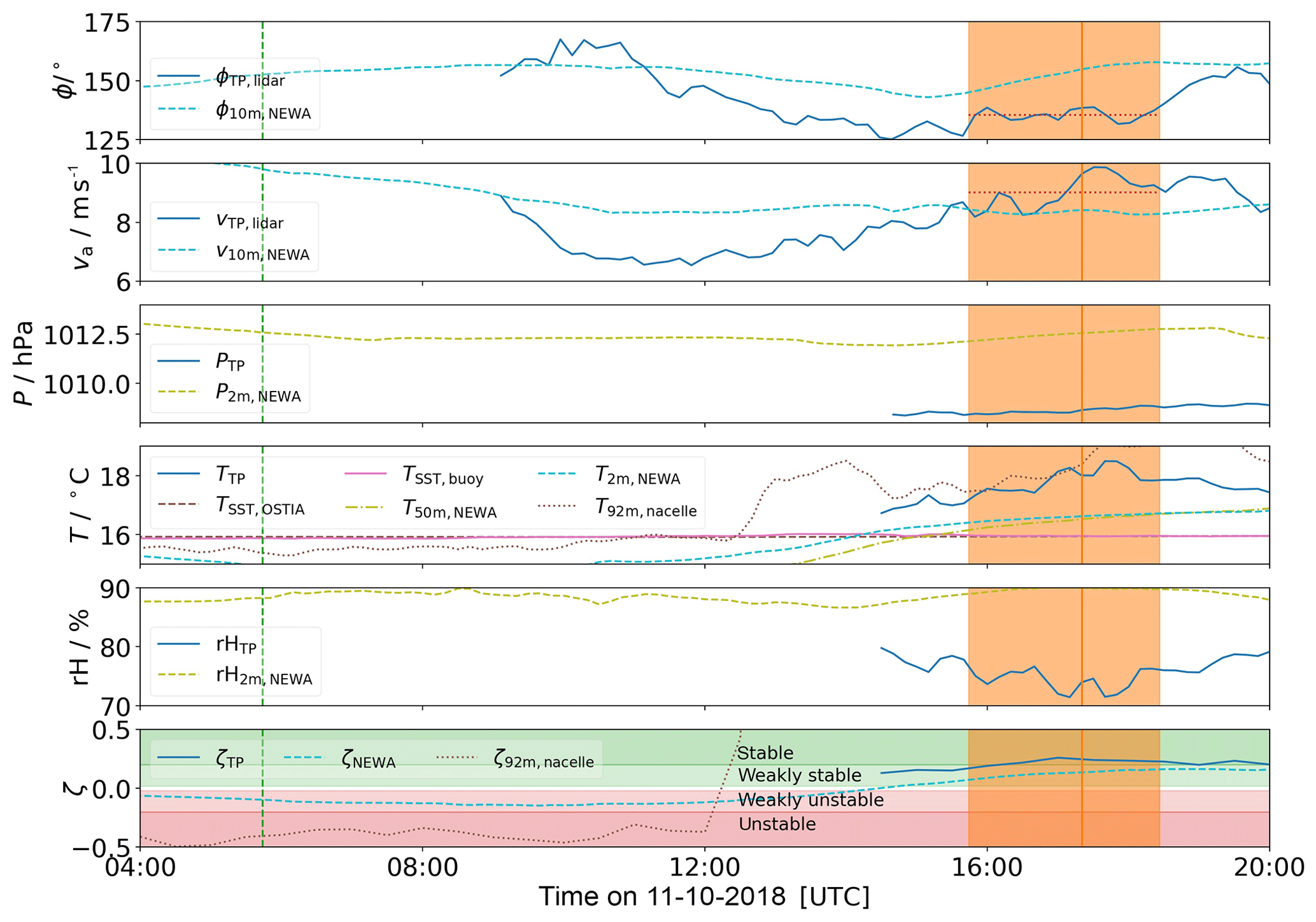
Figure 8Meteorological data at the lidar location (turbine GT58) on 11 October 2018. Top to bottom: wind direction ϕTP,lidar, wind speed vTP,lidar, air pressure PTP, air temperature TTP, sea surface temperatures TSST,OSTIA and TSST,buoy, relative humidity RHTP, and the dimensionless stability parameter ζTP on the height of the TP of GT58 (24.6 m a.m.s.l.). Since the measurements are not available during the whole day, we added the 10 m wind speed v10 m,NEWA and direction ϕ10 m,NEWA, 2 and 50 m temperature T2 m,NEWA and T50 m,NEWA and the stability parameter ζNEWA from the NEWA data set (see Witha et al., 2019) as well as the temperature T92 m,nacelle and the derived stability parameter ζ92 m,nacelle on hub height of turbine GT58. Measurement times are marked as follows: vertical dashed line represents the SAR image (Fig. 9), vertical solid line represents the single lidar scan (Fig. 10), and shaded interval represents the averaged lidar wind field (Fig. 11). Mean wind speed and direction in the averaged lidar interval are marked by red horizontal dotted lines.
We found a good general agreement between the NEWA data and the values measured in the wind farm. Especially the derived stability parameter ζ agrees well. For the differences in the other quantities the different reference heights have to be considered. Half-hourly values of wind speed and direction from the NEWA data are not expected to cover small-scale fluctuations and to perfectly match a local measurement.
3.2.2 SAR wind data
Figure 9a shows the wind field from the Copernicus satellite Sentinel-1A, which passed the German Bight in the morning of 11 October 2018, as an overview of the wind field in the region between GT I and the DolWin2 cluster. The stratification during the SAR snapshot was weakly unstable. Wakes of the Gemini, DolWin1 and DolWin2 clusters with lengths of at least 20, 40 and 55 km, respectively, are clearly visible. The wake originating in the DolWin2 cluster splits into two parts generated by “Gode Wind 1+2” (GW) and Nordsee One (N1); see Fig. 1. The GW wake extends far downstream until it hits the wind farm GT I after approximately 55 km. Further downstream a merged wake of the DolWin2 cluster and GT I can be observed extending out of the visible range after approximately 30 km. All wakes have the approximately same width as the generating cluster and become narrower downstream.
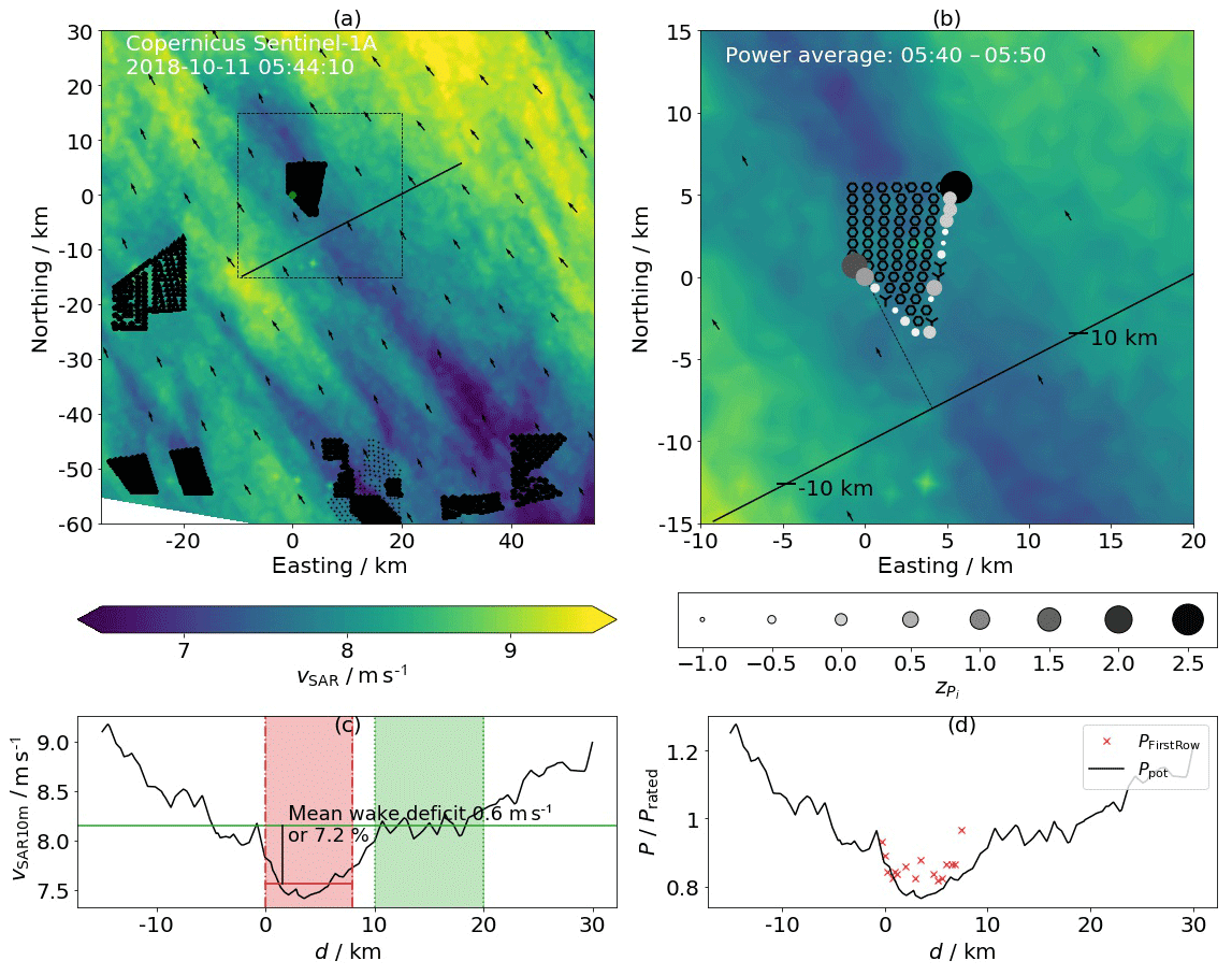
Figure 9Sentinel-1A Ocean Wind Field (Copernicus Sentinel data (2018)); measurement taken 11 October 2018 05:44:10 UTC. We show power data of the upstream turbines in the interval 05:40–05:50 UTC, as in Fig. 5; positions of downstream turbines are marked (hexagon). In (d) we added an offset of 2.0 m s−1 to the SAR wind speeds on the virtual wake cut 9000 m upstream of GT58 before we transferred them to hub height and calculated the potential power. Numbers of considered upstream turbines to calculate the z score are 8, 15, 22, 29, 36, 43, 50, 68, 72, 80, 79, 76, 73, 64, 58, and 51.
The virtual wake cut 9000 m upstream of GT58 reveals regions of different influence (Fig. 9c). On the southwest side of the cut we see a region of undisturbed flow ( km, d is the distance on the wake cut from Fig. 9c) with wind speeds decreasing towards northeast. The deficit between −5 km 0 km originates in the wake of the wind farm N1 followed by the stronger deficit at 0 km 10 km of the GW wind farm. This wake deficit centrally hits GT I and affects its power production. Further east the wind speed remains approximately constant until it rises from d>20 km due to regional differences in the wind field. Regarding the marked wake and free-flow regions in Fig. 9c, we observe a wake deficit of 0.6 m s−1 or 7.2 % in the SAR wind speed for the DolWin2 wake in 10 m height.
Differently from the wake situation of the BorWin cluster (Sect. 3.1), the wind farm GT I is affected by the DolWin wake centrally; therefore, we do not observe separated regions of power production within the farm. Nevertheless, the outer turbines on the western and northeastern corner of the wind farm produce significantly more power (2.6 and 1.7σP above average) than the average of the upstream row (Fig. 9b). Looking at the potential power on hub height calculated from the virtual wake cut (Fig. 9d), we find the increased power to result from the higher wind speeds at the sides of the DolWin2 wake deficit. This highlights the effect of the wake on the power production even in weakly unstable conditions.
3.2.3 Lidar wind fields
In Fig. 10 we show a single lidar scan of the flow southwest of GT I. The stratification during the scan was stable (Fig. 8). We do not observe a sharp transition from wake to free-flow regions like for the BorWin wake (Fig. 6) but a steady decrease in wind speeds southwest to northeast, similar to the DolWin2 wake situation we found in the SAR data from the same morning in weakly unstable stratification (Fig. 9). Three more wakes appear in the wind field: one originating from a ship close to GT I, another one from the OSS Hohe See (×) and the third from the platform BorWin gamma (+). The latter wake extends at least 9 km downstream.
The virtual wake cut (Fig. 10c) highlights the different flow regions with lower wind speeds near GT I. The Hohe See OSS wake is located at km and the BorWin gamma wake between −6 km km. The wake deficit of the DolWin2 cluster amounts to 3.3 m s−1 or 26.4 %. Comparing the potential power in the wind field with the power produced by the turbines of the upstream row, we find most turbines producing approximately rated power (Fig. 10d). The potential power in the west of the wind farm is slightly lower than the power of the upstream turbines. Even though during this lidar scan with high wind speeds the wind farm's power is not influenced by the DolWin2 wake due to the turbines curtailing power production above rated speed, we find clear indications for wake effects with reduced wind speeds at the position of GT I 55 km downstream the DolWin2 cluster.

Figure 10Lidar measurement (scenario A) of the wake of the DolWin2 cluster on 11 October 2018 17:16–17:20 UTC; power data of upstream turbines 17:10–17:20 UTC, as in Fig. 6. Downstream turbine positions marked (hexagon). Turbine numbers to calculate the z score are 8, 15, 22, 29, 36, 43, 50, 68, 72, 78, and 80. Additionally, we marked the converter platform BorWin gamma (+).
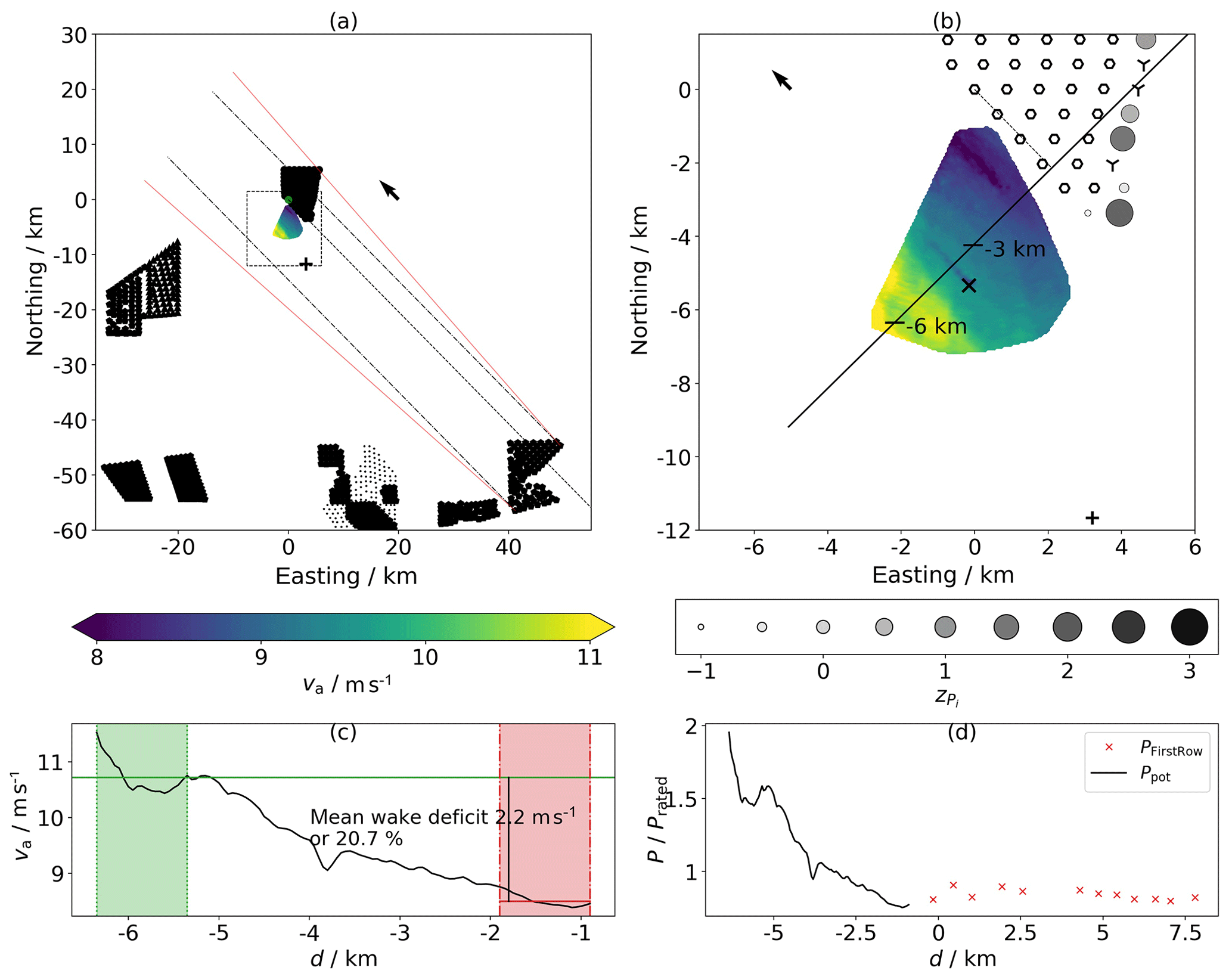
Figure 11Wake of the DolWin2 cluster on 11 October 2018 as in Fig. 6 but averaged over 16 consecutive lidar scans (scan scenario A) in a period of 162 min (15:44–18:26 UTC); power data of upstream turbines averaged over 170 min (15:40–18:30 UTC); downstream turbines marked (hexagon). Turbine numbers to calculate the z score are 8, 15, 22, 29, 36, 43, 50, 68, 72, 78, 80, and 79.
Figure 11 highlights the steadiness of the DolWin2 wake situation on 11 October 2018. We averaged 16 consecutive lidar scans in a period of approximately 162 min (15:44 to 18:26 UTC; cf. shaded interval in Fig. 8) with a relatively constant wind direction. As for the single lidar scan we observe the same behaviour in the wind field with a wind speed decreasing along the virtual wake cut from southwest to northeast. The wake deficits of the Hohe See OSS and BorWin gamma are clearly visible in the averaged wind field (Fig. 11c). The relative wake deficit of the DolWin2 cluster is similar for the single and the averaged lidar scans (Fig. 10). Since the average wind speed within the averaging period is smaller than that at the time of the single scan (Fig. 8), the absolute deficit is smaller, too. The course of the potential power in the wind field (Fig. 11d) is continued by the power of the upstream-rows turbines. The wake effect of the DolWin2 cluster on the power of GT I is evident. The potential power in the wind about 4 km southwest of the wind farm reaches rated wind speed.
We found evidence of cluster wakes in the form of wind speed deficits with clear transition regions between slower wake flow and faster undisturbed flow in many lidar scans upstream of GT I for all neighbouring wind farm clusters in southeasterly to westerly wind directions, namely the DolWin2 (approximately 55 km), DolWin1 (approximately 42 km), Gemini (approximately 54 km) and BorWin (approximately 24 km) clusters. In some of the cases with available large-area SAR wind data, these alternative measurements supported the lidar cluster wake measurements. Power deficits in the wind farm agree with the wake regions found in lidar and SAR data. In this paper we present two exemplary wake cases: one for the BorWin cluster 24 km upstream and one for the DolWin2 cluster 55 km upstream, and both wake effects occurred steadily over more than 2.5 h and influenced the power production of GT I. We found cluster wakes mainly for positive values of the stability parameter ζ (stable stratification) but also for ζ slightly below zero (weakly unstable stratification, shallow boundary layer).
4.1 Influence of cluster wakes on power production of far downstream wind farms
The effect of cluster wakes on the operation of far downstream wind farms has not been investigated before. Nygaard and Hansen (2016) report about short-distance effects in the power production of wind farms in the direct vicinity (3.3 km gap) based on SCADA analysis. Nygaard and Newcombe (2018) analyse a cluster wake at hub height up to 17 km downstream a wind farm with dual Doppler radar from the coast. Platis et al. (2018) find long-reaching wake effects (wind speed difference of more than 0.1 m s−1 considered wakes) up to 55 km downstream in flight measurements but could not analyse their impact on distant wind farms. Here, our findings from combined satellite SAR and lidar measurements of cluster wakes existing over distances of up to 55 km downstream agree with the observation of Platis et al. (2018). Additionally, we confirm the assumption of negative effects of cluster wakes on the power production of a far downstream wind farm.
The evidence of the wake influence on wind farm power is obvious for the BorWin case where we find a clear distinction of wake and free stream in the lidar and SAR wind measurements agreeing with the findings of Platis et al. (2018), who present a wake situation with a high wind speed gradient at one side of the cluster wake. In the BorWin case this edge of the wake continues in a separation of the wind farm turbines' power production (Figs. 5–7). In the DolWin2 case we could argue whether the higher power of the outer turbines (Fig. 9b) result from flow effects at the farm corners leading to higher turbine efficiencies as found by Barthelmie and Jensen (2010) but the comparison of the potential power in the inflow with the turbine power (Fig. 9d) reveals a good agreement, suggesting that at least most of the effect originates in the wake-affected inflow conditions with the highest deficit reducing the power of the central turbines, while the outer turbines profit from higher wind speeds at the sides of the wake.
Wakes are expected to exist far downstream in stable stratifications but to recover much earlier in the unstable case. Platis et al. (2018) report about 41 measurement flights (24× stable, 12× unstable, 5× neutral stratification) and find evidence for cluster wakes in stable boundary layers 55 km downstream, while the furthest evidence in an unstable case is found 10 km downstream. In our lidar measurements we find the most pronounced cluster wakes in stable situations supporting these findings. But we have evidence for far-reaching wakes in neutral and weakly unstable conditions, too. All lidar measurements we present in this work were measured in stable situations but the SAR image of the DolWin2 case (Fig. 9) was taken earlier the same day in a shallow, weakly unstable boundary layer with cluster wakes appearing downstream of many clusters. Vertical momentum transport was possible in lower heights but was hindered by an inversion appearing at approximately 200 to 300 m. The rotor area of the GT I turbines extends up to 150 m height. The DolWin2 wake reaches 55 km downstream until it hits the wind farm GT I where the power production of the upstream-row turbines follows the potential power calculated from the inflow SAR wind. This finding proves the existence of long-reaching cluster wakes and their influence on power production of far downstream wind farms even in cases with weakly unstable stratification. In future work we plan to publish an analysis of the whole data set of the, at the time of writing, still ongoing lidar measurement campaign focusing on wakes in unstable conditions. Nevertheless, the DolWin2 case highlights the necessity to carefully characterize the boundary layer for stability analysis, since the unstable stratified layer in the boundary layer could be thin and limited by an inversion just above temperature measurement height and still within the rotor area.
In addition to the influence of a cluster wake on the wind farm GT I, we still observe inner-farm wake effects (Figs. 5 and 6) with decreasing power production downstream. Cluster wake and wind turbine wakes in the farm overlap. This supports the assumption of the cluster wake being a region of reduced wind speeds with no special characteristics of the original single turbine wakes remaining. We do not perform turbulence analysis comparing cluster wake turbulence to free-flow turbulence in this study. Platis et al. (2018) report a slender wake of increased turbulent kinetic energy (TKE) originating in one corner of the cluster. It was aligned with a stronger horizontal wind speed gradient at the border of the wake. The TKE was reduced in the wake deficit due to the lower wind speeds.
The influence of cluster wakes on the current power production of downstream wind farms could not easily be related to their influence on the annual energy production (AEP). To achieve this, a detailed assessment of the total influence during at least 1 year has to be conducted using, for example, validated wind farm parameterizations in mesoscale models. The local distribution of wind speed, direction and atmospheric stability has to be considered as well as farm and cluster geometries.
In many wake cases the wind speed in the wake deficit still exceeds rated wind speed of the downstream turbines without an effect on their power production. If the upstream cluster's turbines operate in wind speeds above rated speed, their thrust coefficient, cT, decreases additionally, resulting in reduced wake deficits. We expect the total influence of cluster wakes on AEP to be smaller than wake effects from neighbouring wind farms (see Nygaard and Hansen, 2016) due to cluster wake recovery and a smaller wake-influenced wind direction sector. Our findings do not question wind energy utilization of any kind. Nevertheless, a detailed assessment of the influence of cluster wakes on AEP of downstream wind farms during their whole operational life time considering all planned wind energy activities in the region should be conducted in the future. This can improve power production, offshore resource assessment and consequently reduce the uncertainties in financing large offshore wind projects especially in regions with a high level of (planned) wind energy utilization. Therefore, further research is necessary to validate wind farm parameterizations in mesoscale weather models with appropriate wake, power and atmospheric measurements. Especially the influence of atmospheric stability on cluster wake recovery has to be investigated.
Aside from influence on power, the effect on additional wind turbine loads can be relevant. We did not perform analysis of the turbulence in the wake in this study or load simulations on wind turbines affected by far cluster wakes. Since we find sharp edges between wake flow and free stream continuing in the wind farm's power production (Fig. 6), future research should analyse turbine loads dependent on the cluster wake dynamics, e.g. when a turbine on the wake border has to speed up and slow down fast caused by cluster wake dynamics.
4.2 Cluster wake characteristics
Wind turbines are sensitive to the wind conditions over a wide range of heights defined by the swept rotor area. Therefore, the investigation of cluster wakes should cover the whole vertical wind profile at least from lower to upper tip height. Satellite SAR measurements at the sea surface are typically transferred to 10 m height. Platis et al. (2018) investigates cluster wakes at hub height with a research aircraft in stable stratification, and Siedersleben et al. (2018b) additionally presents measurements in five different height levels (60, 90, 120, 150, 220 m) from the same flight, revealing wake deficits in all regarded levels. This highlights a vertical expansion of the wake far above the rotor area (upper tip height: 150 m). We find evidence for cluster wake effects in SAR images (roughness measurement on the sea surface, interpolation to 10 m a.s.l. – above sea level), lidar measurements (≈24.6 m a.m.s.l., 67.0 m below hub height and 9.0 m below lower blade tip height) and from the turbines' power production (rotor swept area spans from 33.6 m to 149.6 m a.m.s.l.). A quantitative comparison of the measured wake strengths is not possible with our data due to the very different type of the measurements. Nevertheless we obtain evidence for wake effects in the boundary layer from the sea surface to the upper tip height 24 and 55 km downstream, agreeing with the observed vertical wake extension closer to the generating cluster presented by Siedersleben et al. (2018b). For a future campaign we suggest the assessment of the development of the atmospheric boundary layer from the inflow through a cluster and in the cluster wake by means of, for example, lidar profilers, lidar range height indicator scans (RHI) or flight measurements for a better understanding of cluster wake development and recovery.
All previous investigations of cluster wakes with satellite SAR suffer from the fact that just one snapshot of the wake is available for a given situation and no wake dynamics or their steadiness could be analysed. Nygaard and Newcombe (2018) investigate a cluster wake at hub height up to 17 km downstream of a wind farm with dual Doppler radar from the coast and present a 1 h average wake field. The aircraft measurements performed by Platis et al. (2018) cover the whole area of the wake along the flight path taking several hours, indicating a constant behaviour of the wake. We find steady wake conditions in both presented examples for more then 2.5 h in the lidar data supported by the corresponding power data. This proves the existence of steady wake effects with a steady influence on the downstream wind farm for constant wind directions. Wake cases with changing wind directions are much harder to analyse since the wake just shortly influences the farm and will probably not even be detectable in wind measurements.
We did not find any evidence for single wind turbine wakes in the lidar inflow measurements of GT I. This is supported by the results by Nygaard and Newcombe (2018), who present dual Doppler radar cross stream flow cuts through a cluster wake at different downstream distances with disappearing signatures of the single turbines from 6 km downstream (unknown stability).
The shapes of the wakes we find could give further hints on the wake recovery process. While shorter wakes (i.e. from the BorWin cluster, Fig. 5) are as wide as the generating cluster, wakes originating further away often appear narrower in the lidar measurements as if they already recovered from the sides or if the whole wake widened with a resulting decrease in maximum wake deficit. This is supported by the shapes of the wakes seen in the SAR wind data in Fig. 9b where the highest wake deficits are narrower further downstream. A detailed analysis of this effect is difficult due to changes in the mesoscale wind field and wakes of neighbouring clusters overlapping with the cluster wake.
The width of the transition region between free flow and wake seems to (at least partly) depend on the downstream position of the wake. In the BorWin wake we sometimes find high wind speed gradients at the wake's border about 20 km downstream (Fig. 6), while in the DolWin wake 50 km downstream the transition region was several kilometres wide (Fig. 10).
The longevity of wakes in stable conditions is further supported by the investigation of two different converter platform wakes in our lidar measurements ranging at least 9 km downstream in one case (Fig. 10). Platform wakes have been observed before, e.g. Chunchuzov et al. (2000) reported a more than 60 km long wake of a 164 m tall offshore platform in very stable atmospheric conditions analysed with satellite SAR measurements. We did not investigate the effect of the wakes of wind farm converter platforms on the power of neighbouring or distant wind turbines but expect it to be fairly small compared to a wind turbine wake due to the lower heights and smaller cross sections of the platforms.
4.3 Cluster wake monitoring
Due to the large areas the cluster wakes take up, their investigation was mainly based on long-ranging remote-sensing techniques. Satellite SAR covers large areas and has been widely used to analyse cluster wakes (Hasager et al., 2015). Our analysis adds the potential power as a computed local quantity to the SAR analysis (Fig. 5d), confirming the wake shape acquired by SAR with turbine power data. This is another hint for the ability of satellite SAR to resolve flow structures, agreeing with the findings of Schneemann et al. (2015), who compared structures in concurrent SAR and lidar measurements indicating the general ability of SAR to resolve flow structures with the size of a few hundred metres.
Cluster wakes have not been measured with long-range lidar. With an achievable maximum range of 10 km with compact devices, lidar seemed not to be appropriate to measure far cluster wakes behind a wind farm. We used lidar to measure incoming far cluster wakes. As opposed to SAR, lidar allows for continuous measurements with scan repetition times in the order of a few minutes (2.5 and 10 min here). In some cases the lidar results are clear (e.g. Fig. 6) but in other cases it is difficult to interpret whether the wind field is influenced by a wake or not. Here, satellite SAR, when available, proves very useful to interpret wind monitoring by lidar offering the possibility to regard the lidar wind field in a wider context (e.g. the DolWin2 case, Sect. 3.2). Nevertheless, absolute wind speed measurements by satellite SAR are comparably imprecise. For the comparison of the shapes of the potential power in the inflow with the turbines' power, we had to correct individual offsets in the SAR wind speeds within the given measurement accuracy. Schneemann et al. (2015) had to correct for an offset in SAR winds, comparing it with lidar, as well. This inaccuracy could be possibly reduced by a SAR analysis tuned to the special case. We did not perform SAR wind calculations ourselves but used already processed wind data.
The analysis of SCADA data on power losses due to cluster wakes without additional flow information from remote sensing is difficult since obvious gradients in wind farm power (Fig. 6) due to cluster wakes are rare and not exactly stationary (e.g. washed out transition region in averaged lidar wind field, Fig. 7b). In the DolWin2 case (Fig. 9) it is hardly possible to judge the contributions of wake effects and effect of higher turbine efficiency at the farm corners (Barthelmie and Jensen, 2010) on the higher power of the turbines at the eastern and western corners of the farm.
For future research on cluster wakes and their influence on power generation, we propose a combination of different measurement techniques complementing with their advantages, namely satellite SAR, long-range lidar and flight measurements (aircrafts and drones). Doppler radar and non-compact lidar systems offering ranges larger than 15 km are available but have not been deployed in offshore wind farms so far due to high costs and technical hurdles in the deployment, orientation and operation of the container-size systems on offshore structures.
Another important aspect of measurements from offshore platforms like transition pieces of offshore wind turbines to be considered is platform movement and the resulting errors in measurement locations. We found platform tilts of up to 0.1∘ due to turbine thrust depending on wind speed and direction using the method of sea surface levelling (Rott et al., 2017). This value might be even higher for turbines on a commonly used monopile foundation compared to the tripod foundation used in GT I. With increasing measurement ranges, the location error in the measurements grows further.
This paper investigates the question of whether offshore cluster wakes have an influence on power generation of far downstream wind farms considering atmospheric stability. Therefore we analysed two different cases of 24 and 55 km long cluster wakes approaching the 400 MW offshore wind farm Global Tech I (GT I) by means of satellite SAR measurements, lidar wind monitoring and analysis of atmospheric stability and GT I power production.
Long-range Doppler lidar supported by satellite SAR proves to be a good combination for cluster wake measurements with the lidar providing accurate wind speed monitoring over long periods and SAR contributing with large-area wind fields for the overall picture.
We find that long-distance wake effects of a wind farm cluster exist at least 55 km downstream in stable and weakly unstable stratification. They persist for more than 2.5 h. During this measurement period the average wake deficits are 2.3 m s−1 or 25 % approximately 24 km downstream and 2.2 m s−1 or 21 % approximately 55 km downstream. Single lidar scans (2.5 min duration) reveal stronger wake deficits of up to 3.9 m s−1 or 41 % approximately 24 km downstream.
Clear transition regions like edges in the wind separate wake and free flow 24 km downstream and continue in the affected wind farm, splitting it into regions of higher power in undisturbed flow and reduced power in the wake deficit. Free-flow turbines produce more then two standard deviations, σP, more than the average of the upstream turbines.
This contribution proves the existence of steady power reductions in a far downstream wind farm caused by cluster wakes. We encourage further investigations on far-reaching wake shadowing effects for optimized areal planning at sea and reduced uncertainties in offshore wind power resource assessment.
Lidar data and meteorological data are published (Schneemann et al., 2019). GT I SCADA data are confidential and therefore not available to the public. SAR wind data are available from https://scihub.copernicus.eu/ (last access: 13 December 2019; Scihub, 2019). Hourly power data for several wind farms are available from https://www.energy-charts.de/ (last access: 19 December 2019; Fraunhofer ISE, 2019). The New European Wind Atlas is published at https://map.neweuropeanwindatlas.eu/ (last access: 19 December 2019; NEWA, 2019). The OSTIA data set can be obtained from http://marine.copernicus.eu/ (last access: 13 December 2019; Copernicus marine service, 2019) and radiosonde soundings are available at
http://www.meteociel.fr/ (last access: 13 December 2019; meteociel.fr, 2019) or
http://weather.uwyo.edu (last access: 13 December 2019; University of Wyoming, 2019).
We derived the virtual potential temperature used in Sect. 2.4 from the available measurements on the TP. We adapted the following methodology mainly from Etling (2008). We need the following:
-
Rd=287 J K−1 kg−1 (specific gas constant of dry air);
-
Rv=461 J K−1 kg−1 (specific gas constant of water vapour);
-
(ratio between the specific gas constants for dry air Rd and water vapour Rv);
-
κP=0.286 (Poisson constant in dry air).
The saturation vapour pressure in pascals (Pa) dependent on the temperature in kelvin (K) follows from the Magnus equation,
The partial pressure of water vapour in the air dependant on the relative humidity RH reads as
while the mixing ratio is
With the specific humidity
and the potential temperature
we approximate the virtual potential temperature as
While the virtual potential temperature at the TP, Θv,TP, could be derived directly from the available measurements, we assume the relative humidity and the air temperature directly above the sea to be RH0=100 % and T0=TSST, respectively, to derive the virtual potential temperature at sea level, Θv,SST. Furthermore we calculate the air pressure at sea level as
assuming a polytropic atmosphere and using the air temperature gradient
JS conducted and supervised the measurement campaign, designed the research, performed the data analysis, made the figures, and planned and wrote the paper. AR and MK contributed to the research with intensive discussions and added to the paper with conceptual discussions and internal review. MD advised on the meteorological parts, participated in the conception of the paper and did an internal review. GS performed parts of the stability analysis and intensively reviewed the article.
The authors declare that they have no conflict of interest.
We acknowledge the wind farm operator Global Tech I Offshore Wind GmbH for providing SCADA data and their support of the work. Furthermore, we thank the European Space Agency (ESA) for making the Sentinel-1 data of the Copernicus programme available. Thanks to the Met Office for making the OSTIA data set available. We acknowledge the NEWA consortium for providing access to the New European Wind Atlas. Special thanks to Stephan Voß for his work on the measurement campaign and the picture from Fig. 3.
The lidar measurements and parts of the work have been supported by the German Federal Ministry for Economic Affairs and Energy on the basis of a decision by the German Bundestag (OWP Control, grant no. 0324131A).
This paper was edited by Rebecca Barthelmie and reviewed by Nicolai Gayle Nygaard and one anonymous referee.
Abkar, M. and Porté-Agel, F.: Influence of atmospheric stability on wind-turbine wakes: A large-eddy simulation study, Phys. Fluids, 27, 035104, https://doi.org/10.1063/1.4913695, 2015. a
Aitken, M. L., Banta, R. M., Pichugina, Y. L., and Lundquist, J. K.: Quantifying Wind Turbine Wake Characteristics from Scanning Remote Sensor Data, J. Atmos. Ocean. Tech., 31, 765–787, https://doi.org/10.1175/JTECH-D-13-00104.1, 2014. a
Barthelmie, R. J. and Jensen, L. E.: Evaluation of wind farm efficiency and wind turbine wakes at the Nysted offshore wind farm, Wind Energy, 13, 573–586, https://doi.org/10.1002/we.408, 2010. a, b, c, d, e
Beck, H. and Kühn, M.: Dynamic Data Filtering of Long-Range Doppler LiDAR Wind Speed Measurements, Remote Sens., 9, 561, https://doi.org/10.3390/rs9060561, 2017. a
Beck, H. and Kühn, M.: Temporal Up-Sampling of Planar Long-Range Doppler LiDAR Wind Speed Measurements Using Space-Time Conversion, Remote Sens., 11, 867, https://doi.org/10.3390/rs11070867, 2019. a
Bodini, N., Zardi, D., and Lundquist, J. K.: Three-dimensional structure of wind turbine wakes as measured by scanning lidar, Atmos. Meas. Tech., 10, 2881–2896, https://doi.org/10.5194/amt-10-2881-2017, 2017. a
Christiansen, M. B. and Hasager, C. B.: Wake effects of large offshore wind farms identified from satellite SAR, Remote Sens. Environ., 98, 251–268, https://doi.org/10.1016/j.rse.2005.07.009, 2005. a
Chunchuzov, I., Vachon, P., and Li, X.: Analysis and Modeling of Atmospheric Gravity Waves Observed in RADARSAT SAR Images, Remote Sens. Environ., 74, 343–361, https://doi.org/10.1016/S0034-4257(00)00076-6, 2000. a
Churchfield, M. J., Lee, S., Michalakes, J., and Moriarty, P. J.: A numerical study of the effects of atmospheric and wake turbulence on wind turbine dynamics, J. Turbulence, 13, N14, https://doi.org/10.1080/14685248.2012.668191, 2012. a
Copernicus marine service: Copernicus Marine environment monitoring service, available at: http://marine.copernicus.eu/, last access: 13 December 2019. a
Donlon, C. J., Martin, M., Stark, J., Roberts-Jones, J., Fiedler, E., and Wimmer, W.: The Operational Sea Surface Temperature and Sea Ice Analysis (OSTIA) system, Remote Sens. Environ., 116, 140–158, https://doi.org/10.1016/j.rse.2010.10.017, 2012. a
Dörenkämper, M., Optis, M., Monahan, A., and Steinfeld, G.: On the Offshore Advection of Boundary-Layer Structures and the Influence on Offshore Wind Conditions, Bound.-Lay. Meteorol., 155, 459–482, https://doi.org/10.1007/s10546-015-0008-x, 2015a. a
Dörenkämper, M., Witha, B., Steinfeld, G., Heinemann, D., and Kühn, M.: The impact of stable atmospheric boundary layers on wind-turbine wakes within offshore wind farms, J. Wind Eng. Indust. Aerodynam., 144, 146–153, https://doi.org/10.1016/j.jweia.2014.12.011, 2015b. a, b
Emeis, S.: A simple analytical wind park model considering atmospheric stability, Wind Energy, 13, 459–469, https://doi.org/10.1002/we.367, 2009. a
Emeis, S.: Wind Energy Meteorology, Springer International Publishing, 2nd Edn, Springer International Publishing AG, part of Springer Nature 2018, https://doi.org/10.1007/978-3-319-72859-9, 2018. a, b
EnBW: EnBW Hohe See and Albatros wind farms, The construction diary for Hohe available at: https://www.enbw.com/renewable-energy/wind-energy/our-offshore-wind-farms/hohe-see/construction-diary.html, (last access: 18 June 2019. a
ESA: Level 2 OCN Ocean Wind Field (OWI) Component, available at: https://sentinel.esa.int/web/sentinel/ocean-wind-field-component, last access: 19 June 2019. a
Etling, D.: Theoretische Meteorologie, 3rd Edn., Springer, Berlin, Heidelberg, https://doi.org/10.1007/978-3-662-10430-9, 2008. a
Fitch, A. C., Olson, J. B., Lundquist, J. K., Dudhia, J., Gupta, A. K., Michalakes, J., and Barstad, I.: Local and Mesoscale Impacts of Wind Farms as Parameterized in a Mesoscale NWP Model, Mon. Weather Rev., 140, 3017–3038, https://doi.org/10.1175/mwr-d-11-00352.1, 2012. a, b, c
Fraunhofer ISE: Energy Charts, available at: https://www.energy-charts.de/, last access: 19 June 2019. a, b
Fuertes, F. C., Markfort, C., and Porté-Agel, F.: Wind Turbine Wake Characterization with Nacelle-Mounted Wind Lidars for Analytical Wake Model Validation, Remote Sens., 10, 668, https://doi.org/10.3390/rs10050668, 2018. a
Grachev, A. A. and Fairall, C. W.: Dependence of the Monin–Obukhov Stability Parameter on the Bulk Richardson Number over the Ocean, J. Appl. Meteorol., 36, 406–414, https://doi.org/10.1175/1520-0450(1997)036<0406:dotmos>2.0.co;2, 1997. a
Hansen, K. S., Barthelmie, R. J., Jensen, L. E., and Sommer, A.: The impact of turbulence intensity and atmospheric stability on power deficits due to wind turbine wakes at Horns Rev wind farm, Wind Energy, 15, 183–196, https://doi.org/10.1002/we.512, 2011. a
Hasager, C., Vincent, P., Badger, J., Badger, M., Bella, A. D., Peña, A., Husson, R., and Volker, P.: Using Satellite SAR to Characterize the Wind Flow around Offshore Wind Farms, Energies, 8, 5413–5439, https://doi.org/10.3390/en8065413, 2015. a, b, c
Hirth, B. D., Schroeder, J. L., Gunter, W. S., and Guynes, J. G.: Coupling Doppler radar-derived wind maps with operational turbine data to document wind farm complex flows, Wind Energy, 18, 529–540, https://doi.org/10.1002/we.1701, 2014. a
Lee, S., Vorobieff, P., and Poroseva, S.: Interaction of Wind Turbine Wakes under Various Atmospheric Conditions, Energies, 11, 1442, https://doi.org/10.3390/en11061442, 2018. a
Li, X. and Lehner, S.: Observation of TerraSAR-X for Studies on Offshore Wind Turbine Wake in Near and Far Fields, IEEE J. Select. Top. Appl. Earth Obs. Remote Sens., 6, 1757–1768, https://doi.org/10.1109/jstars.2013.2263577, 2013. a
Lignarolo, L. E., Mehta, D., Stevens, R. J., Yilmaz, A. E., van Kuik, G., Andersen, S. J., Meneveau, C., Ferreira, C. J., Ragni, D., Meyers, J., van Bussel, G. J., and Holierhoek, J.: Validation of four LES and a vortex model against stereo-PIV measurements in the near wake of an actuator disc and a wind turbine, Renewable Energy, 94, 510–523, https://doi.org/10.1016/j.renene.2016.03.070, 2016. a
Lundquist, J. K., DuVivier, K. K., Kaffine, D., and Tomaszewski, J. M.: Costs and consequences of wind turbine wake effects arising from uncoordinated wind energy development, Nat. Energy, 4, 26–34, https://doi.org/10.1038/s41560-018-0281-2, 2019. a
Mackensen, R.: Windenergie Report Deutschland 2018, available at: http://windmonitor.iee.fraunhofer.de/opencms/export/sites/windmonitor/img/Windmonitor-2018/WERD_2018.pdf, last access: 5 July 2019. a
Merkur Offshore: Sea Change: GE Installs The Last Turbine At One Of Germany's Largest Offshore Wind Farms, available at: https://www.merkur-offshore.com/progress/ (last access: 19 June 2019), 2018. a
meteociel.fr: Observation, Prévisions, Modèles, En temps réel, available at: https://www.meteociel.fr/, last access: 13 December 2019. a
Mouche, A.: Sentinel-1 Ocean Wind Fields (OWI) Algorithm Definition, Tech. Rep. CLS-DAR-NT-10-167 S1-TN-CLS-52-904, CLS/ESA, available at: https://sentinel.esa.int/documents/247904/349449/S-1_L2_OWI_Detailed_Algorithm_Definition.pdf (last access: 22 February 2019), 2011. a
NEWA: New European Wind Atlas, available at: https://map.neweuropeanwindatlas.eu/, last access: 27 June 2019. a, b
Nygaard, N. G.: Wakes in very large wind farms and the effect of neighbouring wind farms, J. Phys.: Conf. Ser., 524, 012162, https://doi.org/10.1088/1742-6596/524/1/012162, 2014. a
Nygaard, N. G. and Hansen, S. D.: Wake effects between two neighbouring wind farms, J. Phys.: Conf. Ser., 753, 032020, https://doi.org/10.1088/1742-6596/753/3/032020, 2016. a, b, c, d
Nygaard, N. G. and Newcombe, A. C.: Wake behind an offshore wind farm observed with dual-Doppler radars, J. Phys.: Conf. Ser., 1037, 072008, https://doi.org/10.1088/1742-6596/1037/7/072008, 2018. a, b, c, d, e, f
Orsted: Borkum Riffgrund 2, available at: https://orsted.de/offshore-windenergie/unsere-offshore-windparks-nordsee/offshore-windpark-borkum-riffgrund-2 (last access: 19 June 2019), 2018. a
Petrofac: BorWin gamma platform topside touches down in the German North Sea, available at: https://www.petrofac.com/en-gb/media/news/borwin-gamma-platform-topside-touches-down-in-the-german-north-sea/ (last access: 7 June 2019), 2018. a
Platis, A., Siedersleben, S. K., Bange, J., Lampert, A., Bärfuss, K., Hankers, R., Cañadillas, B., Foreman, R., Schulz-Stellenfleth, J., Djath, B., Neumann, T., and Emeis, S.: First in situ evidence of wakes in the far field behind offshore wind farms, Scient. Rep., 8, 2163, https://doi.org/10.1038/s41598-018-20389-y, 2018. a, b, c, d, e, f, g, h, i, j, k, l
Pryor, S. C., Barthelmie, R. J., and Shepherd, T. J.: The Influence of Real-World Wind Turbine Deployments on Local to Mesoscale Climate, J. Geophys. Res.-Atmos., 123, 5804–5826, https://doi.org/10.1029/2017jd028114, 2018a. a
Pryor, S. C., Shepherd, T. J., and Barthelmie, R. J.: Interannual variability of wind climates and wind turbine annual energy production, Wind Energ. Sci., 3, 651–665, https://doi.org/10.5194/wes-3-651-2018, 2018b. a
Rodrigo, J. S., Cantero, E., García, B., Borbón, F., Irigoyen, U., Lozano, S., Fernande, P. M., and Chávez, R. A.: Atmospheric stability assessment for the characterization of offshore wind conditions, J. Phys.: Conf. Ser., 625, 012044, https://doi.org/10.1088/1742-6596/625/1/012044, 2015. a
Rott, A., Schneemann, J., Trabucchi, D., Trujillo, J., and Kühn, M.: Accurate deployment of long range scanning lidar on offshore platforms by means of sea surface leveling, in: Poster presentation, NAWEA Windtech, available at: http://windtechconferences.org/wp-content/uploads/2018/01/Windtech2017_AnRott-Poster.pdf (last access: 5 July 2019), 2017. a, b
Schmidt, J. and Stoevesandt, B.: The impact of wake models on wind farm layout optimization, J. Phys.: Conf. Ser., 625, 012040, https://doi.org/10.1088/1742-6596/625/1/012040, 2015. a
Schneemann, J., Hieronimus, J., Jacobsen, S., Lehner, S., and Kühn, M.: Offshore wind farm flow measured by complementary remote sensing techniques: radar satellite TerraSAR-X and lidar windscanners, J. Phys.: Conf. Ser., 625, 012015, https://doi.org/10.1088/1742-6596/625/1/012015, 2015. a, b
Schneemann, J., Voß, S., Rott, A., and Kühn, M.: Doppler wind lidar plan position indicator scans and atmospheric measurements at the offshore wind farm “Global Tech I”, PANGAEA – Data Publisher for Earth & Environmental Science, https://doi.org/10.1594/PANGAEA.909721, 2019. a
Scihub: ESA, Copernicus Open Access Hub, available at: https://scihub.copernicus.eu/, last access: 13 December 2019. a
Siedersleben, S. K., Lundquist, J. K., Platis, A., Bange, J., Bärfuss, K., Lampert, A., Cañadillas, B., Neumann, T., and Emeis, S.: Micrometeorological impacts of offshore wind farms as seen in observations and simulations, Environ. Res. Lett., 13, 124012, https://doi.org/10.1088/1748-9326/aaea0b, 2018a. a
Siedersleben, S. K., Platis, A., Lundquist, J. K., Lampert, A., Bärfuss, K., Cañadillas, B., Djath, B., Schulz-Stellenfleth, J., Bange, J., Neumann, T., and Emeis, S.: Evaluation of a Wind Farm Parametrization for Mesoscale Atmospheric Flow Models with Aircraft Measurements, Meteorol. Z., 27, 401–415, https://doi.org/10.1127/metz/2018/0900, 2018b. a, b, c
Sorbjan, Z. and Grachev, A. A.: An Evaluation of the Flux-Gradient Relationship in the Stable Boundary Layer, Bound.-Lay. Meteorol., 135, 385–405, https://doi.org/10.1007/s10546-010-9482-3, 2010. a
Trabucchi, D., Trujillo, J.-J., and Kühn, M.: Nacelle-based Lidar Measurements for the Calibration of a Wake Model at Different Offshore Operating Conditions, Energy Procedia, 137, 77–88, https://doi.org/10.1016/j.egypro.2017.10.335, 2017. a
Turner, S., Romero, D., Zhang, P., Amon, C., and Chan, T.: A new mathematical programming approach to optimize wind farm layouts, Renew. Energy, 63, 674–680, https://doi.org/10.1016/j.renene.2013.10.023, 2014. a
University of Wyoming: Wyoming weather web, available at: http://weather.uwyo.edu/, last access: 13 December 2019. a
Vincent, P., Bourbigot, M., Johnsen, H., and Piantanida, R.: Sentinel-1 Product Specification, Tech. Rep. S1-RS-MDA-52-7441, ESA, available at: https://sentinel.esa.int/web/sentinel/user-guides/sentinel-1-sar/document-library/-/asset_publisher/1dO7RF5fJMbd/content/sentinel-1-product-specification, last access: 13 December 2019. a, b
Volker, P. J. H., Badger, J., Hahmann, A. N., and Ott, S.: The Explicit Wake Parametrisation V1.0: a wind farm parametrisation in the mesoscale model WRF, Geosci. Model Dev., 8, 3715–3731, https://doi.org/10.5194/gmd-8-3715-2015, 2015. a
Vollmer, L., Steinfeld, G., Heinemann, D., and Kühn, M.: Estimating the wake deflection downstream of a wind turbine in different atmospheric stabilities: an LES study, Wind Energ. Sci., 1, 129–141, https://doi.org/10.5194/wes-1-129-2016, 2016. a
Witha, B., Hahmann, A., Sīle, T., Dörenkämper, M., Ezber, Y., García-Bustamante, E., González-Rouco, J. F., Leroy, G., and Navarro, J.: WRF model sensitivity studies and specifications for the NEWA mesoscale wind atlas production runs, Technical report, The NEWA consortium, 73 pp., https://doi.org/10.5281/zenodo.2682604, 2019. a, b, c