Rossby number similarity of an atmospheric RANS model using limited-length-scale turbulence closures extended to unstable stratification

The design of wind turbines and wind farms can be improved by increasing the accuracy of the inflow models representing the atmospheric boundary layer. In this work we employ one-dimensional Reynolds-averaged Navier–Stokes (RANS) simulations of the idealized atmospheric boundary layer (ABL), using turbulence closures with a length-scale limiter. These models can represent the mean effects of surface roughness, Coriolis force, limited ABL depth, and neutral and stable atmospheric conditions using four input parameters: the roughness length, the Coriolis parameter, a maximum turbulence length, and the geostrophic wind speed. We find a new model-based Rossby similarity, which reduces the four input parameters to two Rossby numbers with different length scales. In addition, we extend the limited-length-scale turbulence models to treat the mean effect of unstable stratification in steady-state simulations. The original and extended turbulence models are compared with historical measurements of meteorological quantities and profiles of the atmospheric boundary layer for different atmospheric stabilities.

1 Introduction

Wind turbines operate in the turbulent atmospheric boundary layer (ABL) but are designed with simplified inflow conditions that represent analytic wind profiles of the atmospheric surface layer (ASL). The ASL corresponds to roughly the first 10 % of the ABL, typically less than 100 m, while the tip heights of modern wind turbines are now sometimes beyond 200 m. Hence, there is a need for inflow models that represent the entire ABL in order to improve the design of wind turbines and wind farms. Such a model should be simple enough to efficiently improve the chain of design tools used by the wind energy industry.

The ABL is complex and changes continuously over time. Idealized, steady-state models can represent long-term-averaged velocity and turbulence profiles of the real ABL, including the effects of Coriolis, atmospheric stability, capping inversion, homogeneous surface roughness and flat terrain; here we exclude the effects of flow inhomogeneity and nonstationarity, which are typically considered by mesoscale and three-dimensional time-varying models. In this work, we investigate idealized ABL models that are based on one-dimensional Reynolds-averaged Navier–Stokes (RANS) equations, where the only spatial dimension is the height above ground. The output of the model can be used as inflow conditions for three-dimensional RANS simulations of complex terrain (Koblitz et al., 2015) and wind farms (van der Laan and Sørensen, 2017b). Turbulence is modeled here by two limited-length-scale turbulence closures, the mixing-length model of Blackadar (1962) and the two-equation k–ε model of Apsley and Castro (1997). These turbulence models can simulate one-dimensional stable and neutral ABLs without the necessity of a temperature equation and a momentum source term of buoyancy. In other words, all temperature effects are represented by the turbulence model. The limited-length-scale turbulence models depend on four parameters: the roughness length, the Coriolis parameter, the geostrophic wind speed, and a chosen maximum turbulence length scale that is related to the ABL depth. We show that the normalized profiles of wind speed, wind direction and turbulence quantities are only dependent on two dimensionless parameters that represent the ratio of the inertial to the Coriolis force, based on two different length scales: the roughness length and the maximum turbulence length scale. These dimensionless parameters are Rossby numbers. The Rossby number based on the roughness length is known as the surface Rossby number, as introduced by Lettau (1959), while the Rossby number based on the maximum turbulence length is a new dimensionless parameter. The obtained model-based Rossby number similarity is used to validate a range of simulations with historical measurements of the geostrophic drag coefficient and cross-isobar angle. In addition, we show that both RANS models' solutions are bounded by two analytic solutions of the idealized ABL.

The limited-length-scale turbulence closures of Blackadar (1962) and Apsley and Castro (1997) can model the effect of stable and neutral stability but cannot model the unstable atmosphere. We propose simple extensions to solve this issue and validate the results of the extended k–ε model with measurements of wind speed and wind direction profiles. The model extensions lead to a third Rossby number, where the length scale is based on the Obukhov length. The limited mixing-length model is not considered in the comparison with measurements because we are mainly interested in the limited-length-scale k–ε model. The k–ε model is more applicable to wind energy applications because it can also provide an estimate of the turbulence intensity, which is not available from the limited mixing-length model of Blackadar (1962). The limited mixing-length model is applied here to show that the same model-based Rossby number similarity as obtained for the k–ε model is recovered.

The article is structured as follows. The background and theory of the idealized ABL are discussed in Sect. 2. Extensions to unstable surface layer stratification are presented in Sect. 3. Section 4 presents the methodology of the one-dimensional RANS simulations. The model-based Rossby similarity is illustrated in Sect. 5. The simulation results of the limited-length-scale k–ε model including the extension to unstable conditions are compared with measurements in Sect. 6.

2 Background and theory – idealized models of the ABL

We model the mean steady-state flow in an idealized ABL. Here idealized refers to flow over homogeneous and flat terrain under barotropic conditions such that the geostrophic wind does not vary with height. This flow can be described by the incompressible RANS equations for momentum, where the contribution from the molecular viscosity is neglected due to the high Reynolds number:

$$\begin{array}{}\text{(1)}& \begin{array}{rl}& {\displaystyle \frac{\mathrm{D}U}{\mathrm{D}t}}=f_{\mathrm{c}}\left(V-V_{\mathrm{G}}\right)+{\displaystyle \frac{\mathrm{d}}{\mathrm{d}z}}\left({\mathit{\nu }}_T{\displaystyle \frac{\mathrm{d}U}{\mathrm{d}z}}\right)=\mathrm{0},\\ & {\displaystyle \frac{\mathrm{D}V}{\mathrm{D}t}}=-f_{\mathrm{c}}\left(U-U_{\mathrm{G}}\right)+{\displaystyle \frac{\mathrm{d}}{\mathrm{d}z}}\left({\mathit{\nu }}_T{\displaystyle \frac{\mathrm{d}V}{\mathrm{d}z}}\right)=\mathrm{0},\end{array}\end{array}$$

where U and V are the mean horizontal velocity components, U_G and V_G are the corresponding mean geostrophic velocities, f_c=2Ωsin (λ) is the Coriolis parameter with Ω as Earth's angular velocity and λ as the latitude, and z is the height above ground. In addition, the Reynolds stresses $\stackrel{\mathrm{‾}}{u^{\prime }{w}^{\prime }}$ and $\stackrel{\mathrm{‾}}{v^{\prime }{w}^{\prime }}$ are modeled by the linear stress–strain relationship of Boussinesq (1897): $\stackrel{\mathrm{‾}}{u^{\prime }{w}^{\prime }}=-{\mathit{\nu }}_T\mathrm{d}U/\mathrm{d}z$ and $\stackrel{\mathrm{‾}}{v^{\prime }{w}^{\prime }}=-{\mathit{\nu }}_T\mathrm{d}V/\mathrm{d}z$, where ν_T is the eddy viscosity. The boundary conditions for U and V are $U=V=\mathrm{0}$ at z=z₀ and U=U_G and V=V_G at z→∞, where z₀ is the roughness length. Note that it is possible to write the two momentum equations as a single ordinary differential equation:

$$\begin{array}{}\text{(2)}& {\displaystyle \frac{\mathrm{d}}{\mathrm{d}z}}\left({\mathit{\nu }}_T{\displaystyle \frac{\mathrm{d}W}{\mathrm{d}z}}\right)=i{f}_{\mathrm{c}}W,\end{array}$$

where $W\equiv (U-U_{\mathrm{G}})+i(V-V_{\mathrm{G}})$ is a complex variable and $i^{\mathrm{2}}=-\mathrm{1}$.

The eddy viscosity, ν_T, needs to be modeled in order to close the system of equations. The eddy viscosity can be written as ${\mathit{\nu }}_T=u_{*}\mathrm{\ell }$, where u_* and ℓ represent turbulence velocity and turbulence length scales. For a constant eddy viscosity, the equations can be solved analytically, and the solution is known as the Ekman spiral (Ekman, 1905), which includes the wind direction change with height due to Coriolis effects. The Ekman spiral can also be considered a laminar solution, since one can neglect the turbulence in the momentum equations and set the molecular viscosity to determine the rate of mixing. For an eddy viscosity that increases linearly with height, the equations can also be solved analytically, as introduced by Ellison (1956) and discussed by Krishna (1980) and Constantin and Johnson (2019). The two analytic solutions are provided in Appendix A. One can relate the analytic solution of Ellison (1956) to the (neutral) ASL (z≪z_i), while the Ekman spiral is more valid for altitudes around the ABL depth z_i. Neither of the two analytic solutions result in a realistic representation of the entire (idealized) ABL. A combination of both a linear eddy viscosity for z≪z_i and a constant eddy viscosity for z∼z_i should provide a more realistic solution. For example, the eddy viscosity could have the form ${\mathit{\nu }}_T=\mathit{\kappa }{u}_{*\mathrm{0}}z\exp (-z/h)$, where ν_T increases linearly with height for z≪h as expected in the surface layer; then it reaches a maximum value at z=h, and decreases to zero for z>h. Note that u_*0 is the friction velocity near the surface. Constantin and Johnson (2019) derived a number of solutions for a variable eddy viscosity, although an explicit solution for the entire idealized ABL with a realistic eddy viscosity (in the previously mentioned form) has not been found yet. Hence, numerical methods are still necessary, and one of the simplest numerical models for the idealized ABL is given by Blackadar (1962) using Prandtl's mixing-length model:

$$\begin{array}{}\text{(3)}& {\mathit{\nu }}_T={\mathrm{\ell }}^{\mathrm{2}}\mathcal{S},\end{array}$$

where $\mathcal{S}=\sqrt{(\mathrm{d}U/\mathrm{d}z{)}^{\mathrm{2}}+(\mathrm{d}V/\mathrm{d}z{)}^{\mathrm{2}}}=|\mathrm{d}W/\mathrm{d}z|$ is the magnitude of the strain-rate tensor, and  ℓ is prescribed as a turbulence length scale,

$$\begin{array}{}\text{(4)}& \mathrm{\ell }={\displaystyle \frac{\mathit{\kappa }z}{\mathrm{1}+\frac{\mathit{\kappa }z}{{\mathrm{\ell }}_{\max }}}},\end{array}$$

where κz is the turbulence length scale in the neutral surface layer with κ as the von Kármán constant, and ℓ_max is a maximum turbulence length scale. It is also possible to model the eddy viscosity with a two-equation turbulence closure, e.g., the k–ε model:

$$\begin{array}{}\text{(5)}& {\mathit{\nu }}_T=C_{\mathit{\mu }}{\displaystyle \frac{k^{\mathrm{2}}}{\mathit{\epsilon }}},\end{array}$$

with C_μ as a model parameter, k as the turbulent kinetic energy, and ε as the dissipation of k. Both k  and ε are modeled by a transport equation:

$$\begin{array}{}\text{(6)}& {\displaystyle }& {\displaystyle \frac{\mathrm{D}k}{\mathrm{D}t}}={\displaystyle \frac{\mathrm{d}}{\mathrm{d}z}}\left({\displaystyle \frac{{\mathit{\nu }}_T}{{\mathit{\sigma }}_k}}{\displaystyle \frac{\mathrm{d}k}{\mathrm{d}z}}\right)+\mathcal{P}-\mathit{\epsilon },\text{(7)}& {\displaystyle }& {\displaystyle \frac{\mathrm{D}\mathit{\epsilon }}{\mathrm{D}t}}={\displaystyle \frac{\mathrm{d}}{\mathrm{d}z}}\left({\displaystyle \frac{{\mathit{\nu }}_T}{{\mathit{\sigma }}_{\mathit{\epsilon }}}}{\displaystyle \frac{\mathrm{d}\mathit{\epsilon }}{\mathrm{d}z}}\right)+\left(C_{\mathit{\epsilon },\mathrm{1}}\mathcal{P}-C_{\mathit{\epsilon },\mathrm{2}}\mathit{\epsilon }\right){\displaystyle \frac{\mathit{\epsilon }}{k}},\end{array}$$

where 𝒫 is the turbulence production, and σ_k, σ_ε, C_ε,1, and C_ε,2 are model constants that should follow the relationship ${\mathit{\kappa }}^{\mathrm{2}}={\mathit{\sigma }}_{\mathit{\epsilon }}\sqrt{C_{\mathit{\mu }}}(C_{\mathit{\epsilon },\mathrm{2}}-C_{\mathit{\epsilon },\mathrm{1}})$. When using the standard k–ε model calibrated for atmospheric flows (Richards and Hoxey, 1993), the turbulence length scale or eddy viscosity will keep increasing until a boundary layer depth is formed and the analytic solution of Ellison (1956) is approximated. Apsley and Castro (1997) proposed modifying the transport equation of ε, such that a maximum turbulence length scale is enforced by replacing the constant C_ε,1 with a variable parameter $C_{\mathit{\epsilon },\mathrm{1}}^{*}$:

$$\begin{array}{}\text{(8)}& C_{\mathit{\epsilon },\mathrm{1}}^{*}=C_{\mathit{\epsilon },\mathrm{1}}+\left(C_{\mathit{\epsilon },\mathrm{2}}-C_{\mathit{\epsilon },\mathrm{1}}\right){\displaystyle \frac{\mathrm{\ell }}{{\mathrm{\ell }}_{\max }}},\end{array}$$

where the turbulence length scale is modeled as $\mathrm{\ell }=C_{\mathit{\mu }}^{\mathrm{3}/\mathrm{4}}{k}^{\mathrm{3}/\mathrm{2}}/\mathit{\epsilon }$. This limited-length-scale k–ε model behaves very similarly to the mixing-length model of Blackadar (1962) (Eqs. 3 and 4). For ℓ≪ℓ_max, the surface layer solution is obtained, while for ℓ∼ℓ_max, the source terms in the transport equation of ε cancel each other out ($C_{\mathit{\epsilon },\mathrm{1}}^{*}\mathcal{P}\sim C_{\mathit{\epsilon },\mathrm{1}}\mathit{\epsilon }$), and the turbulence length scale is limited. For a given z₀, G, and f_c, the ABL depth can be controlled by ℓ_max. This means that ℓ_max is related to z_i; Apsley and Castro (1997) noted that ${\mathrm{\ell }}_{\max }\sim z_i/\mathrm{3}$ applies to typical neutral ABLs. However, the simulated boundary layer depth using the k–ε model of Apsley and Castro (1997) has an approximate dependence of $z_i\propto (G/|f_{\mathrm{c}}|{)}^{\mathrm{1}-a}{\mathrm{\ell }}_{\max }^a$ with a≈0.6, which we will further discuss in Sect. 5. A summary of the discussed eddy viscosity closures is listed in Table 1. Figure 1 compares the analytic solutions of Ekman (1905) and Ellison (1956) with the numerical solutions of the limited mixing-length model of Blackadar (1962) and the limited-length-scale k–ε of Apsley and Castro (1997) in terms of wind speed, wind direction, $\mathit{\theta }=\arctan (V/U)$, and eddy viscosity. The Ekman spiral is depicted with two constant eddy viscosities, which only translates the solution vertically. In addition, we have chosen $f_{\mathrm{c}}={\mathrm{10}}^{-\mathrm{4}}$ s⁻¹, G=10 m s⁻¹, and $z_{\mathrm{0}}={\mathrm{10}}^{-\mathrm{2}}$ m. The numerical solutions are shown for a range of ℓ_max values. It is clear that the ABL depth decreases for lower values of ℓ_max, for both numerical models, and their solutions behave similarly. A lower ℓ_max also results in a higher shear and wind veer and a lower eddy viscosity, which are characteristics of a stable ABL. Hence, the limited-length-scale turbulence closures can model the effects of stable stratification by solely limiting the turbulence length scale, without the need of a temperature equation or buoyancy source terms. When ℓ_max→0 m (note that there is minimal limit of ℓ_max in order to obtain numerically stable results), the solution approaches the Ekman spiral because the eddy viscosity in the ABL can be approximated by a constant eddy viscosity. Hence, the maximum change in wind direction simulated by the k–ε model of Apsley and Castro (1997) is that of the Ekman spiral: 45^∘. For large ℓ_max values, the numerical solution approximates the analytic solution of Ellison (1956) but does not match it because their eddy viscosities are different for z≥z_i.

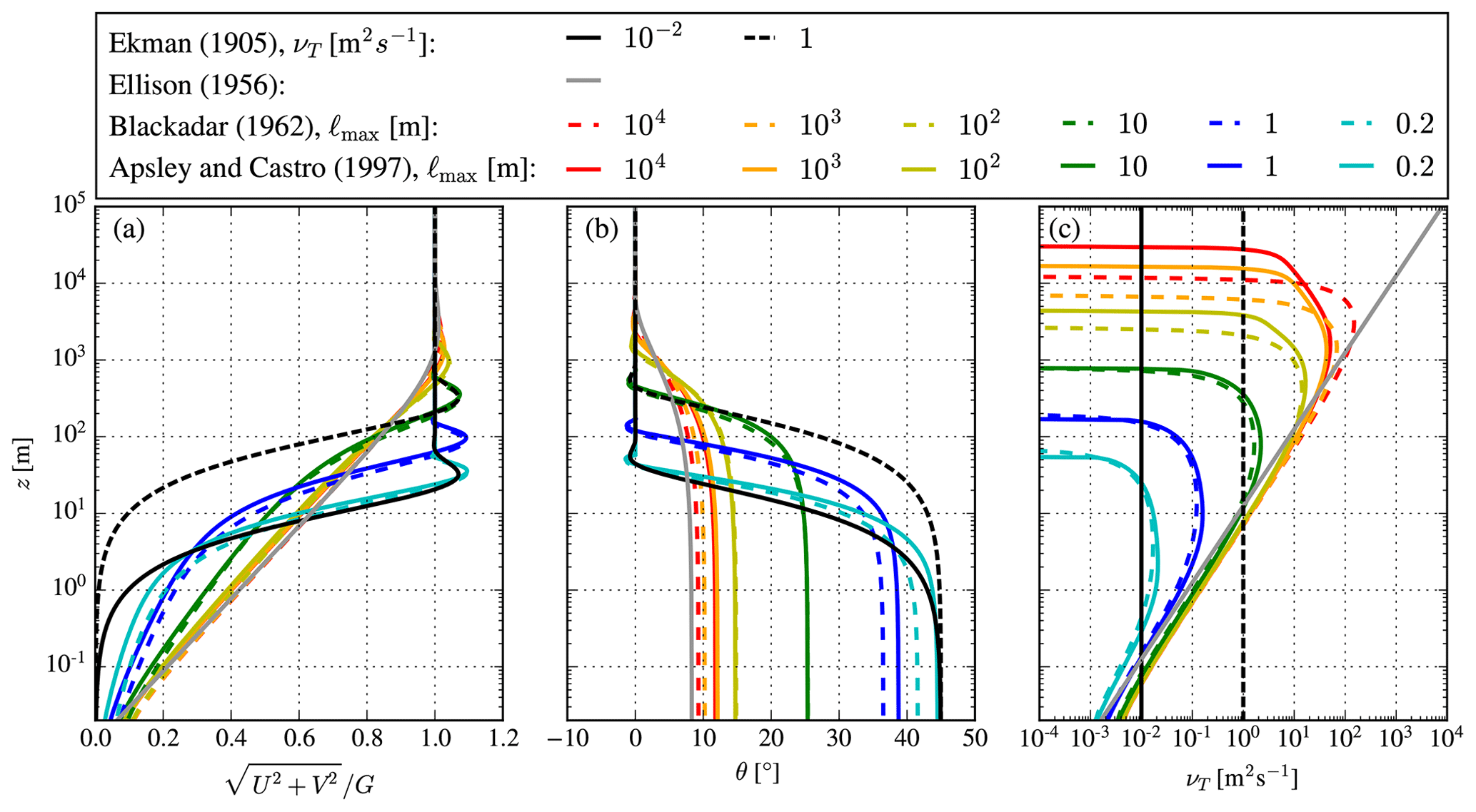
Figure 1 Comparison of analytic and numerical solutions of existing idealized ABL models using $f_{\mathrm{c}}={\mathrm{10}}^{-\mathrm{4}}$ s⁻¹, G=10 m s⁻¹, and $z_{\mathrm{0}}={\mathrm{10}}^{-\mathrm{2}}$ m for different model parameters. (a) Wind speed. (b) Wind direction. (c) Eddy viscosity.

Ekman (1905)Ellison (1956)Blackadar (1962)Apsley and Castro (1997)

Table 1 Eddy viscosity closures for the idealized ABL.

3 Extension to unstable surface layer stratification

The two limited-length-scale turbulence closures discussed in Sect. 2 can be used to model neutral and stable ABLs without the need of a temperature equation and buoyancy forces. However, it is not possible to model the unstable ABL because the turbulence length scale is only limited, not enhanced, i.e., ℓ≤κz. In order to model unstable conditions, we need to extend the models such that the turbulence length scale is enhanced in the surface layer, ℓ>κz, which we present in the following sections for each turbulence closure.

3.1 Limited mixing-length model

One can generically parameterize the turbulence length scale ℓ as a “parallel” combination of ASL and ABL scales,

$$\begin{array}{}\text{(9)}& {\displaystyle \frac{\mathrm{1}}{\mathrm{\ell }}}={\displaystyle \frac{\mathrm{1}}{{\mathrm{\ell }}_{\mathrm{ASL}}}}+{\displaystyle \frac{\mathrm{1}}{{\mathrm{\ell }}_{\mathrm{ABL}}}}.\end{array}$$

Blackadar (1962) chose ℓ_ASL=κz and ℓ_ABL=ℓ_max to arrive at Eq. (4). If we choose to set

$$\begin{array}{}\text{(10)}& {\mathrm{\ell }}_{\mathrm{ASL}}={\displaystyle \frac{\mathit{\kappa }z}{{\mathit{\varphi }}_{\mathrm{m}}}}\end{array}$$

following the turbulence length scale that is a result of Monin–Obukhov Similarity Theory (MOST, Monin and Obukhov, 1954) – where

$$\begin{array}{}\text{(11)}& {\mathit{\varphi }}_{\mathrm{m}}={\left(\mathrm{1}-{\mathit{\gamma }}_{\mathrm{1}}z/L\right)}^{-\mathrm{1}/\mathrm{4}}\end{array}$$

is the dimensionless velocity gradient for unstable conditions, with γ₁≈16 as shown by Dyer (1974), and L is the Obukhov length – then it is possible to extend the limited mixing-length model of Blackadar (1962) to unstable surface layer stratification, as

$$\begin{array}{}\text{(12)}& \mathrm{\ell }={\displaystyle \frac{\mathit{\kappa }z}{{\left(\mathrm{1}-{\mathit{\gamma }}_{\mathrm{1}}z/L\right)}^{-\mathrm{1}/\mathrm{4}}+\mathit{\kappa }z/{\mathrm{\ell }}_{\max }}}.\end{array}$$

Approaching neutral conditions, $L^{-\mathrm{1}}\to \mathrm{0}$, the original length-scale model of Blackadar (1962) is obtained. Note that in stable conditions, ${\mathit{\varphi }}_{\mathrm{m}}=\mathrm{1}+\mathit{\beta }z/L$, so the resulting turbulence length can also be rewritten in the form of Eqs. (4) and (9), using an effective maximum turbulence length scale of

$$\begin{array}{}\text{(13)}& {\mathrm{\ell }}_{\mathrm{ABL},\mathrm{stable}}^{-\mathrm{1}}={\mathrm{\ell }}_{\max ,\mathrm{eff}}^{-\mathrm{1}}\equiv {\mathrm{\ell }}_{\max }^{-\mathrm{1}}+\mathit{\beta }/\left(\mathit{\kappa }L\right).\end{array}$$

Thus we can simply use the original length-scale model of Blackadar (1962) for stable and neutral conditions; the stable ϕ_m function simply informs the selection of ℓ_max,eff, following Eq. (13).

3.2 Limited-length-scale k–ε model

Sumner and Masson (2012) argued that, in stable conditions, the limited-length-scale k–ε model of Apsley and Castro (1997) overpredicts ℓ in the surface layer compared to MOST, where ${\mathrm{\ell }}_{\max }=L\mathit{\kappa }/\mathit{\beta }$ and β≈5. They proposed a more complicated expression for $C_{\mathit{\epsilon },\mathrm{1}}^{*}$ in the transport equation of ε compared to the original model of Apsley and Castro (1997). Sogachev et al. (2012) alternatively prescribed a coefficient in the buoyant term of the ε equation, depending on ℓ∕ℓ_max and being similar to the production-related term that gives results consistent (at least asymptotically) with MOST. We find that the correction of Sumner and Masson (2012) provides a better match of the turbulence length scale within the surface layer compared to MOST with respect to the original k–ε model of Apsley and Castro (1997). However, we also find that a larger overshoot of the turbulence length scale around the ABL depth is found when Coriolis is included. Alternatively, one could improve the surface layer solution of the original model of Apsley and Castro (1997) by simply reducing ℓ_max by roughly 20 %. Therefore, we choose to use the model of Apsley and Castro (1997) as our starting point.

In order to account for the increase in turbulence length scale in the surface layer under unstable conditions, we add a buoyancy source term ℬ in the k–ε transport equations:

$$\begin{array}{}\text{(14)}& {\displaystyle }& {\displaystyle \frac{\mathrm{D}k}{\mathrm{D}t}}={\displaystyle \frac{\mathrm{d}}{\mathrm{d}z}}\left({\displaystyle \frac{{\mathit{\nu }}_T}{{\mathit{\sigma }}_k}}{\displaystyle \frac{\mathrm{d}k}{\mathrm{d}z}}\right)+\mathcal{P}-\mathit{\epsilon }+\mathcal{B},\text{(15)}& {\displaystyle }& {\displaystyle \frac{\mathrm{D}\mathit{\epsilon }}{\mathrm{D}t}}={\displaystyle \frac{\mathrm{d}}{\mathrm{d}z}}\left({\displaystyle \frac{{\mathit{\nu }}_T}{{\mathit{\sigma }}_{\mathit{\epsilon }}}}{\displaystyle \frac{\mathrm{d}\mathit{\epsilon }}{\mathrm{d}z}}\right)+\left(C_{\mathit{\epsilon },\mathrm{1}}^{*}\mathcal{P}-C_{\mathit{\epsilon },\mathrm{2}}\mathit{\epsilon }+C_{\mathit{\epsilon },\mathrm{3}}^{*}\mathcal{B}\right){\displaystyle \frac{\mathit{\epsilon }}{k}}.\end{array}$$

Here ℬ is modeled as

$$\begin{array}{}\text{(16)}& \mathcal{B}=-{\mathit{\nu }}_T\left[{\left({\displaystyle \frac{\mathrm{d}U}{\mathrm{d}z}}\right)}^{\mathrm{2}}+{\left({\displaystyle \frac{\mathrm{d}V}{\mathrm{d}z}}\right)}^{\mathrm{2}}\right]{\displaystyle \frac{z}{L}},=-{\mathit{\nu }}_T{\mathcal{S}}^{\mathrm{2}}{\displaystyle \frac{z}{L}}\end{array}$$

following MOST, using the similarity functions of Dyer (1974) as discussed in van der Laan et al. (2017). We use the flow-dependent parameter $C_{\mathit{\epsilon },\mathrm{3}}^{*}\equiv \mathrm{1}+{\mathit{\alpha }}_B(C_{\mathit{\epsilon },\mathrm{1}}-C_{\mathit{\epsilon },\mathrm{2}})$ of Sogachev et al. (2012), which for unstable conditions includes the prescription

$$\begin{array}{}\text{(17)}& {\mathit{\alpha }}_B=\mathrm{1}-\left[\mathrm{1}+{\displaystyle \frac{\left(C_{\mathit{\epsilon },\mathrm{2}}-\mathrm{1}\right)}{\left(C_{\mathit{\epsilon },\mathrm{2}}-C_{\mathit{\epsilon },\mathrm{1}}\right)}}\right]{\displaystyle \frac{\mathrm{\ell }}{{\mathrm{\ell }}_{\max }}},\end{array}$$

amenable to the free-convection limit: $\mathit{\epsilon }/\mathcal{B}\to \mathrm{1}$ for $\mathcal{P}/\mathcal{B}\to \mathrm{0}$. Further, α_B→1 as ℓ→0, matching neutral conditions since z∕L also vanishes then. The prescription (Eq. 17) results in

$$\begin{array}{}\text{(18)}& C_{\mathit{\epsilon },\mathrm{3}}^{*}=\mathrm{1}+C_{\mathit{\epsilon },\mathrm{1}}-C_{\mathit{\epsilon },\mathrm{2}}+\left(\mathrm{2}{C}_{\mathit{\epsilon },\mathrm{2}}-C_{\mathit{\epsilon },\mathrm{1}}-\mathrm{1}\right){\displaystyle \frac{\mathrm{\ell }}{{\mathrm{\ell }}_{\max }}},\end{array}$$

which also means that $C{*}_{\mathit{\epsilon },\mathrm{3}}\to C_{\mathit{\epsilon },\mathrm{2}}$ approaching the effective ABL top (ℓ→ℓ_max), so sources and sinks of ε balance in Eq. (15), i.e., $\mathcal{P}-\mathit{\epsilon }+\mathcal{B}$, all have the same coefficient C_ε,2.

4 Methodology of numerical simulations

The one-dimensional numerical simulations are performed with EllipSys1D (van der Laan and Sørensen, 2017a), which is a simplified one-dimensional version of EllipSys3D, initially developed by Sørensen (1994) and Michelsen (1992). EllipSys1D is a finite volume solver for incompressible flow, with collocated storage of flow variables. It is assumed that the vertical velocity is zero and the pressure gradients are constant, which is valid in an idealized ABL, as discussed in Sect. 2. As a consequence, it is not necessary to solve the pressure correction equation that is normally used to ensure mass conservation.

4.1 Ambient turbulence in the limited-length-scale k–ε turbulence model

The limited-length-scale k–ε model typically simulates an eddy viscosity that decays to zero for z→∞, which can lead to numerical instability. While, for example, Koblitz et al. (2015) chose to set upper limits for k and ε to prevent numerical instabilities, we prefer a more physical method, including ambient source terms S_k,amb and S_ε,amb in the k and ε transport equations, respectively. Following Spalart and Rumsey (2007), we set

$$\begin{array}{}\text{(19)}& S_{k,\mathrm{amb}}={\mathit{\epsilon }}_{\mathrm{amb}},S_{\mathit{\epsilon },\mathrm{amb}}=C_{\mathit{\epsilon },\mathrm{2}}{\displaystyle \frac{{\mathit{\epsilon }}_{\mathrm{amb}}^{\mathrm{2}}}{k_{\mathrm{amb}}}}.\end{array}$$

When all sources of turbulence are zero ($\mathcal{P}=B=\mathrm{0}$) and the diffusion terms are zero ($\mathrm{d}k/\mathrm{d}z=\mathrm{d}\mathit{\epsilon }/\mathrm{d}z=\mathrm{0}$), then k=k_amb and ε=ε_amb. To be consistent with the equations solved, we define the ambient turbulence quantities in terms of the driving parameters, G and ℓ_max:

$$\begin{array}{}\text{(20)}& \begin{array}{rl}& {\mathrm{\ell }}_{\mathrm{amb}}=C_{\mathrm{amb}}{\mathrm{\ell }}_{\max },k_{\mathrm{amb}}={\displaystyle \frac{\mathrm{3}}{\mathrm{2}}}{I}_{\mathrm{amb}}^{\mathrm{2}}{G}^{\mathrm{2}},\\ & {\mathit{\epsilon }}_{\mathrm{amb}}=C_{\mathit{\mu }}^{\mathrm{3}/\mathrm{4}}{\displaystyle \frac{k_{\mathrm{amb}}^{\frac{\mathrm{3}}{\mathrm{2}}}}{{\mathrm{\ell }}_{\mathrm{amb}}}}=C_{\mathit{\mu }}^{\mathrm{3}/\mathrm{4}}{\displaystyle \frac{\mathrm{3}}{\mathrm{2}}}\sqrt{{\displaystyle \frac{\mathrm{3}}{\mathrm{2}}}}{\displaystyle \frac{I_{\mathrm{amb}}^{\mathrm{3}}}{C_{\mathrm{amb}}}}{\displaystyle \frac{G^{\mathrm{3}}}{{\mathrm{\ell }}_{\max }}}.\end{array}\end{array}$$

Here I_amb is the total turbulence intensity¹ above the (simulated) ABL, and C_amb is the ratio of the turbulence length scale above the ABL (ℓ_amb) to maximum turbulence length scale (ℓ_max). We choose small values for $I_{\mathrm{amb}}={\mathrm{10}}^{-\mathrm{6}}$ and $C_{\mathrm{amb}}={\mathrm{10}}^{-\mathrm{6}}$, such that the ambient turbulence does not affect the solution for U and V, while the numerical stability is maintained. It should be noted that the overshoot in ℓ∕ℓ_max that can occur near the ABL depth is still affected by the ambient values. Sogachev et al. (2012) and Koblitz et al. (2015) chose to use a limiter on ε to avoid an overshoot in ℓ, but we choose not to use it. In general, we prefer to avoid limiters because they can break the Rossby number similarity that is presented in Sect. 5.

4.2 Numerical setup

The flow is driven by a constant pressure gradient using a prescribed constant geostrophic wind speed. The initial wind speed is set to the geostrophic wind speed at all heights. During the solving procedure, the ABL depth grows from the ground until convergence is achieved, which occurs when the growth rate of the ABL depth is negligible because a balance between the prescribed pressure gradient, the Coriolis forces, and the turbulence stresses is obtained. The flow that we are solving is relatively stiff, and we choose to include the transient terms using a second-order three-level implicit method with a large time step that is set as $\mathrm{1}/\left|f_{\mathrm{c}}\right|$ s. All spatial gradients are discretized by a second-order central-difference scheme. Convergence is typically achieved after 10⁵ iterations, which takes about 10 s on a single 2.7 GHz CPU. The domain height is set to 10⁵ m to ensure that the ABL depth is significantly smaller than the domain height for all flow cases considered. The numerical grid represents a line, where the first cell height is set to 10⁻² m. The cells are stretched for increasing heights using an expansion ratio of about 1.2. The grid consists of 384 cells, which is based on a grid refinement study presented in Sect. 4.3. A rough-wall boundary condition is set at the ground, as discussed by Sørensen et al. (2007). For the length-scale-limited k–ε model, this means that we set ε at the first cell, use a Neumann condition for k, and the shear stress at the wall is defined by the neutral surface layer. The first cell is placed on top of the roughness length, which allows us to choose the first cell height independent of the roughness length. This means that we add the roughness length to all relations that include z, i.e., z+z₀. For the limited mixing-length model, we simply set the eddy viscosity from the neutral surface layer at the first cell. Neumann conditions are set for all flow variables at the top boundary.

The turbulence model constants of the k–ε model are set as (C_μ, σ_k, σ_ε, C_ε,1, C_ε,2, κ)=(0.03, 1.0, 1.3, 1.21, 1.92, 0.4). The chosen C_μ value is based on neutral ASL measurements, as discussed by Richards and Hoxey (1993), and C_ε,1 is used to maintain the neutral ASL solution of the k–ε model.

4.3 Grid refinement study

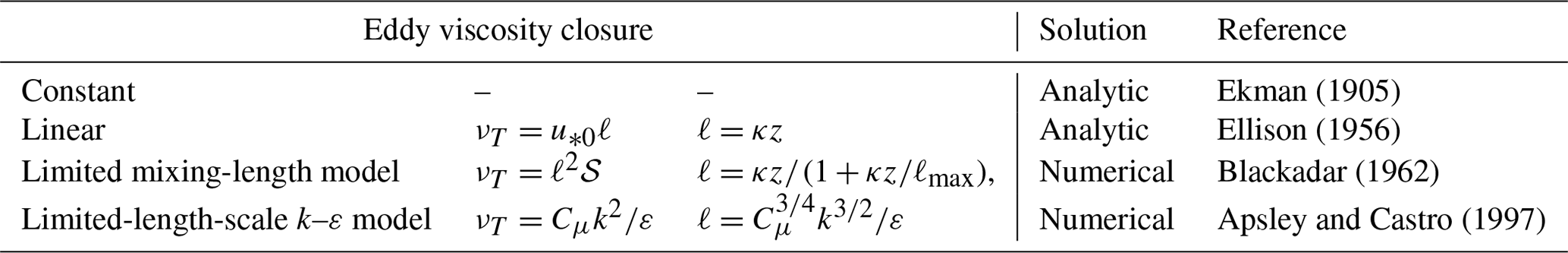
A grid refinement study of the numerical setup is performed for the limited-length-scale k–ε model of Apsley and Castro (1997), using 48, 96, 192, 384, and 768 cells. We choose $f_{\mathrm{c}}={\mathrm{10}}^{-\mathrm{4}}$ s⁻¹, $z_{\mathrm{0}}={\mathrm{10}}^{-\mathrm{4}}$ m, and G=10 m s⁻¹ for ℓ_max=100 and ℓ_max=1 m. The results in terms of the wind speed of each grid are depicted in Fig. 2 for both values of ℓ_max. For ℓ_max=100 m, the largest difference with respect to the finest grid is 0.5 %, 0.2 %, 0.09 %, and 0.03 % for 48, 96, 192, and 384 cells, respectively, located at the first cell near the wall boundary. When using ℓ_max=1 m, a small ABL depth of 100 m is simulated with a sharp low-level jet. In the enlarged plot of Fig. 2b, one can see how the grid size affects the low-level jet, where the largest difference with respect to the finest grid is 1 %, 0.2 %, 0.04 %, and 0.01 %, for 48, 96, 192, and 384 cells, respectively. We find similar results for the limited mixing-length model of Blackadar (1962). In addition, the turbulence model extensions to unstable surface layer stratification typically show smaller differences between the grids due to the enhanced mixing and the use of a high ℓ_max value that represents a convective ABL. Hence, our choice of using 384 cells is conservative.

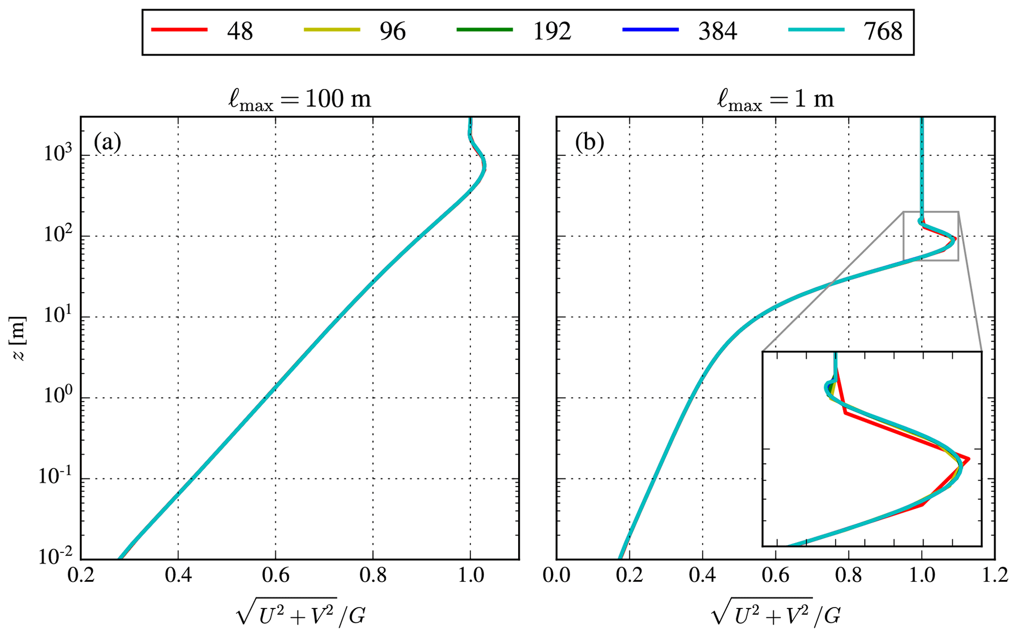
Figure 2 Grid refinement study of the one-dimensional RANS simulation using the limited-length-scale k–ε model, for 48, 96, 192, 384, and 768 cells. (a) ℓ_max=100 m. (b) ℓ_max=1 m.

5 Rossby number similarity in numerical and analytical solutions

The numerical solution of the original limited-length-scale turbulence closures of Blackadar (1962) and Apsley and Castro (1997) depend on four parameters: f_c (s⁻¹), G (m s⁻¹), ℓ_max (m), and z₀ (m). Applying the Buckingham π theorem, it is clear that there should exist two dimensionless numbers that define the entire solution, since the four dimensional parameters only have two dimensions (meters and seconds). This can be shown by writing a nondimensional momentum equation in complex form (Eq. 2) using the nondimensional variables $W^{\prime }\equiv W/\mathcal{U}$, ${\mathit{\nu }}_{T_{\mathrm{0}}}\equiv {\mathit{\nu }}_T/\left(\mathcal{U}\mathcal{L}\right)$ and $z_{\mathrm{0}}\equiv z/\mathcal{L}$, where 𝒰 and ℒ are characteristic velocity and length scales, respectively:

$$\begin{array}{}\text{(21)}& Ro{\displaystyle \frac{\mathrm{d}}{\mathrm{d}{z}^{\prime }}}\left({\mathit{\nu }}_T^{\prime }{\displaystyle \frac{\mathrm{d}{W}^{\prime }}{\mathrm{d}{z}^{\prime }}}\right)=i{W}^{\prime }.\end{array}$$

Here, Ro is the Rossby number, $Ro=\mathcal{U}/\left(\right|f_{\mathrm{c}}\left|\mathcal{L}\right)$, which describes the ratio of the inertial (advective) tendency to the Coriolis force. If we apply the original mixing-length model of Blackadar (1962) for ${\mathit{\nu }}_T^{\prime }$ using Eqs. (3) and (4), then Eq. (21) can be written as

$$\begin{array}{}\text{(22)}& Ro{\displaystyle \frac{\mathrm{d}}{\mathrm{d}{z}^{\prime }}}\left({\left[{\displaystyle \frac{\mathit{\kappa }{z}^{\prime }}{\mathrm{1}+\mathit{\kappa }{z}^{\prime }\mathcal{L}/{\mathrm{\ell }}_{\max }}}\right]}^{\mathrm{2}}\left|{\displaystyle \frac{\mathrm{d}{W}^{\prime }}{\mathrm{d}{z}^{\prime }}}\right|{\displaystyle \frac{\mathrm{d}{W}^{\prime }}{\mathrm{d}{z}^{\prime }}}\right)=i{W}^{\prime },\end{array}$$

where $-\mathcal{L}/{\mathrm{\ell }}_{\max }$, is a second dimensionless number. If we choose 𝒰=G and ℒ=z₀, we may define two Rossby-like numbers, with characteristic length scales based on z₀ and ℓ_max, respectively:

$$\begin{array}{}\text{(23)}& R{o}_{\mathrm{0}}\equiv {\displaystyle \frac{G}{\left|f_{\mathrm{c}}\right|z_{\mathrm{0}}}},R{o}_{\mathrm{\ell }}\equiv {\displaystyle \frac{G}{\left|f_{\mathrm{c}}\right|{\mathrm{\ell }}_{\max }}}.\end{array}$$

Here, we have obtained Ro_ℓ by rewriting the second dimensionless number ℒ∕ℓ_max as the ratio of the two Rossby numbers: $\mathcal{L}/{\mathrm{\ell }}_{\max }=[\mathcal{U}/(\left|f_{\mathrm{c}}\right|{\mathrm{\ell }}_{\max }\left)\right]/[\mathcal{U}/(\left|f_{\mathrm{c}}\right|\mathcal{L}\left)\right]$. Ro₀ is known as the surface Rossby number, first introduced by Lettau (1959); it also resembles a ratio of (inertial) boundary layer depth to z₀. Analogously, Ro_ℓ is like the ratio of two boundary layer depths, $f_{\mathrm{c}}/u_{*\mathrm{0}}$ and z_i (e.g., Arya and Wyngaard, 1975); here ℓ_max is a proxy for z_i, acting as a “lid” for the ABL. Considering Eq. (23), we have reduced the number of dependent parameters from four to two: f(f_c, G, ℓ_max, z₀)→f(Ro₀, Ro_ℓ). For a fixed surface roughness z₀, the ratio of the two Rossby numbers is then the only dependent parameter:

$$\begin{array}{}\text{(24)}& {\mathrm{\ell }}_{\max }={\displaystyle \frac{R{o}_{\mathrm{0}}}{R{o}_{\mathrm{\ell }}}}{z}_{\mathrm{0}};\end{array}$$

i.e., the ratio of simulated ABL depth to z₀ is the lone parameter. Blackadar (1962) found a characteristic maximum ABL turbulence length scale of 0.00027 $G/\left|f_{\mathrm{c}}\right|$ for the Leipzig wind profile (Lettau, 1950), which equating with ℓ_max corresponds to Ro_ℓ≃3700.

Figure 3 depicts the Rossby number similarity of our one-dimensional RANS simulations using the original limited-length-scale turbulence closures of Blackadar (1962), Fig. 3a–c, and Apsley and Castro (1997), Fig. 3d–g. Four combinations of Ro₀ (10⁶ and 10⁹) and Ro_ℓ (10³ and 10⁵) are used, each simulated with four combinations of G (10 and 20 m s⁻¹) and f_c ($\mathrm{5}\times {\mathrm{10}}^{-\mathrm{5}}$ and 10⁻⁴ s⁻¹). The roughness length and maximum turbulence length scale follow from Eq. (23) and cover a wide range of z₀ from 10⁻⁴ to 0.4 m and ℓ_max of 100–400 m. Figure 3 shows that normalized wind speed, wind direction, and turbulence quantities for both turbulence closures are only dependent on Ro₀ and Ro_ℓ. Both turbulence closures produce similar results in terms of wind speed, wind direction, and eddy viscosity. The limited-length-scale k–ε model of Apsley and Castro (1997) also predicts a total turbulence intensity I (Fig. 3g) and a turbulence length scale ℓ (not shown in Fig. 3), which are only dependent on the two Rossby numbers. In addition, the total turbulence intensity close to the surface only depends on Ro₀, while further away, it is mainly influenced by Ro_ℓ with a weaker dependence on Ro₀.

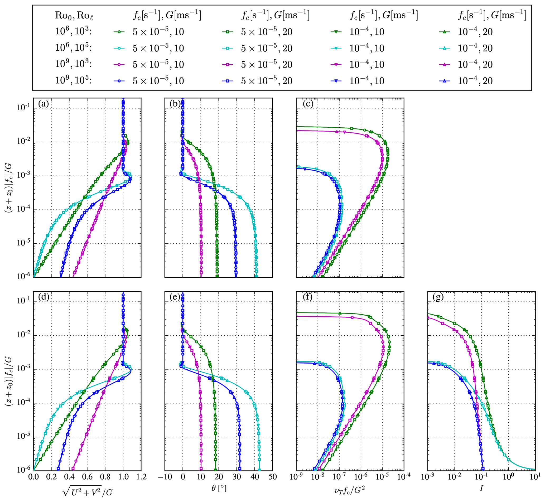
Figure 3 Rossby number similarity of the original turbulence closures. (a–c) Limited mixing-length model. (d–g) Limited-length-scale k–ε model.

Considering the non-neutral ABL with Coriolis effects but ignoring the strength of capping inversion (entrainment), in the micrometeorological literature the Kazanskii and Monin (1961) parameter $u_{*\mathrm{0}}/\left(\right|f_{\mathrm{c}}\left|L\right)$ is typically invoked (e.g., Arya, 1975; Zilitinkevich, 1989). This can also be considered as a third Rossby number, which in our context of using G instead of u_*0 is

$$\begin{array}{}\text{(25)}& R{o}_{L_{-}}\equiv {\displaystyle \frac{-G}{\left|f_{\mathrm{c}}\right|L}};\end{array}$$

here the subscript (${}_{L_{-}}$) denotes that Eq. (25) is defined for unstable conditions, i.e., L≤0. For the convective boundary layer, $u_{*\mathrm{0}}/(-|f_{\mathrm{c}}\left|L\right)$ is generally replaced by the dimensionless inversion height $-z_i/L$, because the convective ABL depth does not have a significant dependence on $u_{*\mathrm{0}}/f_{\mathrm{c}}$ (Arya, 1975). However, we note that $R{o}_{L_{-}}$ functions as a “bottom-up” parameter in the non-neutral RANS equation set, with the Obukhov length L in Eq. (16) specified as a surface layer quantity; in effect $R{o}_{L_{-}}$ dictates the relative increase in mixing length (i.e., in the dimensionless coordinate $z\left|f_{\mathrm{c}}\right|/G$). Our length-scale-limited turbulence closures extended to unstable surface layer stratification, as presented in Sect. 3, are dependent on $R{o}_{L_{-}}$. This becomes clear when we substitute the mixing-length model extended to unstable surface layer stratification from Eq. (12) into the nondimensional momentum equation from Eq. (21):

$$\begin{array}{}\text{(26)}& Ro{\displaystyle \frac{\mathrm{d}}{\mathrm{d}{z}^{\prime }}}\left({\left[{\displaystyle \frac{\mathit{\kappa }{z}^{\prime }}{{\left(\mathrm{1}-{\mathit{\gamma }}_{\mathrm{1}}{z}^{\prime }\mathcal{L}/L\right)}^{-\mathrm{1}/\mathrm{4}}+\mathit{\kappa }{z}^{\prime }\mathcal{L}/{\mathrm{\ell }}_{\max }}}\right]}^{\mathrm{2}}\left|{\displaystyle \frac{\mathrm{d}{W}^{\prime }}{\mathrm{d}{z}^{\prime }}}\right|{\displaystyle \frac{\mathrm{d}{W}^{\prime }}{\mathrm{d}{z}^{\prime }}}\right)=i{W}^{\prime },\end{array}$$

where ℒ∕L is a third nondimensional number, which can also be written as the ratio of two Rossby numbers: $R{o}_{L_{-}}/R{o}_{\mathrm{0}}$. For $R{o}_{L_{-}}=\mathrm{0}$, the extended models return to the original models. Figure 4 depicts the Rossby number similarity of the extended turbulence closures using six combinations of the three Rossby numbers, which are each simulated with four combinations of G and f_c. We use two values of Ro₀ (10⁶ and 10⁹) and three values of $R{o}_{L_{-}}$ (0, 5×10², and 2×10³) for Ro_ℓ=10³. For these Rossby number combinations, $R{o}_{L_{-}}=\mathrm{5}\times {\mathrm{10}}^{\mathrm{2}}$ and $R{o}_{L_{-}}=\mathrm{2}\times {\mathrm{10}}^{\mathrm{3}}$ correspond to near-unstable conditions ($-\mathrm{1}/L=\mathrm{0.00125}$–0.005 m⁻¹) and unstable to very unstable conditions ($-\mathrm{1}/L=\mathrm{0.005}$–0.02 m⁻¹), respectively. Figure 4 shows that both extended turbulence closures only depend on Ro₀ and $R{o}_{L_{-}}$ for a given Ro_ℓ. Although not shown in Fig. 4, changing Ro_ℓ would not break the Rossby number similarity. Note that it does not make sense to include combinations of nonzero values of $R{o}_{L_{-}}$ that correspond to unstable conditions and large values of Ro_ℓ that correspond to stable conditions.

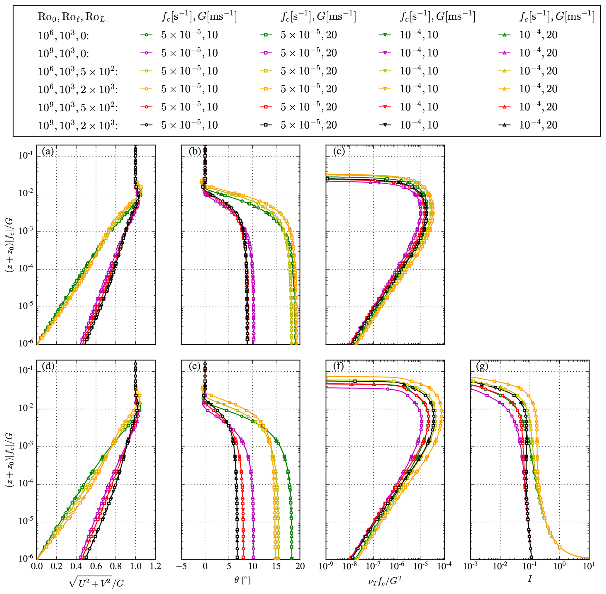
Figure 4 Rossby number similarity of the turbulence closures extended to unstable surface layer conditions. (a–c) Limited mixing-length model. (d–g) Limited-length-scale k–ε model.

The extended limited-length-scale mixing-length model (Fig. 4a–c) is less sensitive to $R{o}_{L_{-}}$ compared to the extended limited-length-scale k–ε model (Fig. 4d–g) because of the buoyancy production in the transport equations of k and ε, which is not present in the extended mixing-length model. Both models predict a deeper ABL (larger z_i) that is more mixed for stronger unstable surface layer stratification (increasing $R{o}_{L_{-}}$). The wind veer is also reduced in stronger unstable conditions for the extended k–ε model (Fig. 4e), but it does not always decrease with increasing unstable conditions for the extended mixing-length model (Fig. 4b).

One could choose to use the friction velocity at the surface, u_*0, as a velocity scale in the Rossby numbers instead of the geostrophic wind speed. However, the friction velocity depends on height z and is a result of the model, not an input. In other words, the height at which the friction velocity needs to be extracted to obtain a collapse is also dependent on the ABL profiles, since the height scales with friction velocity. Hence it is more sensible to use geostrophic wind speed as a velocity scale in the model-based Rossby number similarity – consistent also with classic Ekman theory (which relates the wind speed in terms of G). Nevertheless, it is possible to obtain a Rossby similarity using u_*0 as the velocity scale, which is presented in Appendix B.

The Rossby number similarity can be employed to generate a library of ABL profiles for a range of Ro₀, Ro_ℓ, and $R{o}_{L_{-}}$. The library contains all possible model solutions for the range of chosen Rossby numbers, and it can be used to determine inflow profiles for three-dimensional RANS simulations, without the need for running one-dimensional precursor simulations.

The obtained Rossby number similarity can only be achieved for a grid-independent numerical setup, as we have shown in Sect. 4.3. In addition, the ambient source terms should also be scaled by the relevant input parameters (G and ℓ_max), as discussed in Sect. 4.1.

The ABL depth z_i predicted by the original limited-length-scale turbulence closures is mainly dependent on the maximum turbulence length scale ℓ_max. The normalized ABL depth ($(z_i+z_{\mathrm{0}})\left|f_{\mathrm{c}}\right|/G$) is mainly dependent on Ro_ℓ, which is depicted in Fig. 5, where results of the limited-length-scale k–ε model extended to unstable surface layer stratification are shown for $\mathrm{3}\times \mathrm{6}\times \mathrm{3}$ combinations of the three Rossby numbers Ro₀, Ro_ℓ, and $R{o}_{L_{-}}$. We have chosen G=10 m s⁻¹ and $f_{\mathrm{c}}={\mathrm{10}}^{-\mathrm{4}}$ s⁻¹, but the results are independent of G and f_c due to the Rossby number similarity. The normalized ABL depth is defined as the height at which the wind direction (relative to the geostrophic wind direction) becomes zero for the second time, i.e., above the mean jet and associated turning as in Ekman theory. For the Ekman solution (Sect. A1), this definition results in an ABL depth equal to $z_i=\mathrm{2}\mathit{\pi }\sqrt{\mathrm{2}{\mathit{\nu }}_T/\left|f_{\mathrm{c}}\right|}$. The normalized ABL depth in the RANS model increases for stronger unstable surface layer conditions (larger $R{o}_{L_{-}}$), i.e., for larger values of the surface heat flux. For neutral and stable conditions ($R{o}_{L_{-}}=\mathrm{0}$) and moderate to shallow ABL depths, i.e., $\mathrm{3}\times {\mathrm{10}}^{\mathrm{3}}\le R{o}_{\mathrm{\ell }}\le \mathrm{3}\times {\mathrm{10}}^{\mathrm{4}}$ – corresponding to $z_i<\sim \mathrm{2000}$ m as seen in Fig. 5 – we find that ${\log }_{\mathrm{10}}\left(\right[z_i+z_{\mathrm{0}}\left]\right|f_{\mathrm{c}}|/G)\propto -a{\log }_{\mathrm{10}}\left(R{o}_{\mathrm{\ell }}\right)$, with a=0.57–0.62 for Ro₀ over the range of 10⁹–10⁵. Hence for moderate to shallow ABLs the effective depth modeled in neutral and stable conditions is roughly $z_i\propto {\mathrm{\ell }}_{\max }^a(G/|f_{\mathrm{c}}|{)}^{\mathrm{1}-a},$ with a≈0.6. As seen by the solid lines in Fig. 5, under neutral conditions and with large ABL depths, the z_i dependence on ℓ_max softens ($a<\mathrm{2}/\mathrm{3}$) and deviates from a power law, while for unstable conditions a is similar to the previously found value of 0.6.

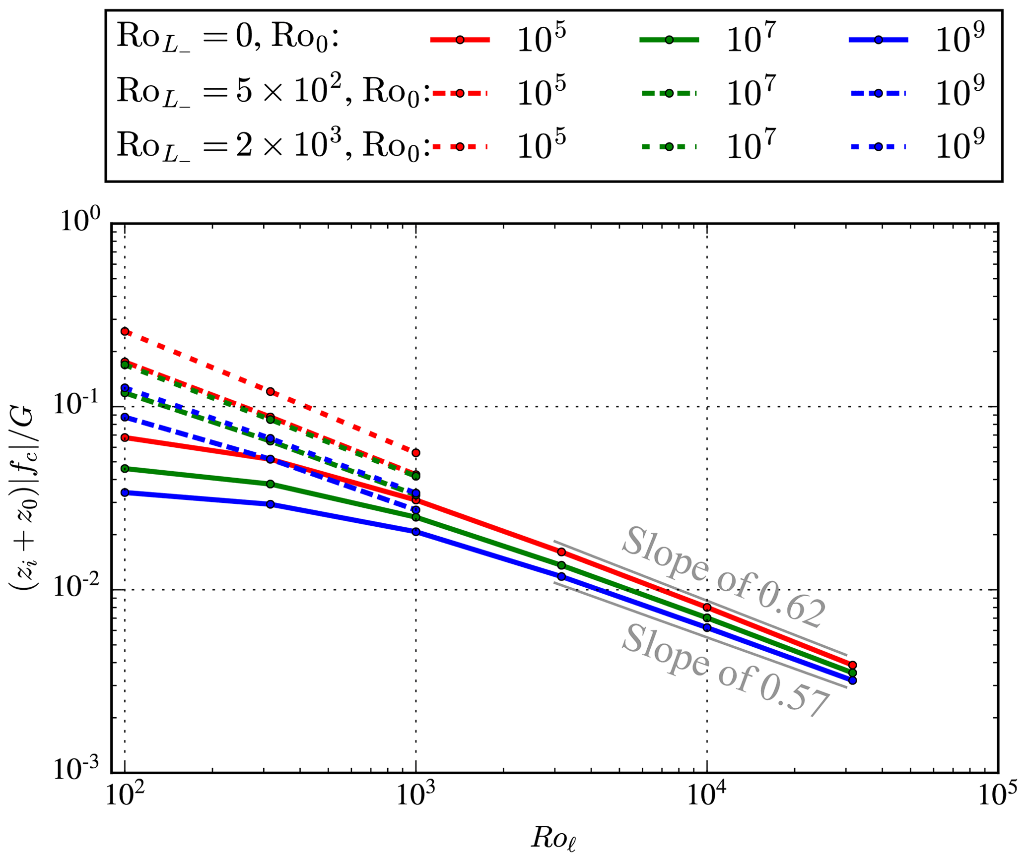
Figure 5 Normalized boundary layer depth z_i predicted by limited-length-scale k–ε model extended to unstable surface layer stratification, as a function of the three Rossby numbers.

6 Validation and model limits

We employ the Rossby similarity from Sect. 5 to validate a range of results simulated by the original limited-length-scale k–ε model of Apsley and Castro (1997) including our proposed extension to unstable surface layer stratification. Historical measurements of the geostrophic drag coefficient $u_{*\mathrm{0}}/G$ and the cross-isobar angle (the angle between the surface wind direction and the geostrophic wind direction), as summarized by Hess and Garratt (2002), and measured profiles of the ASL and ABL for different atmospheric stabilities from Peña et al. (2010, 2014), respectively, are used as validation metrics. The limited mixing-length model of Blackadar (1962) and its extension are not considered in the comparison with measurements, since we are mainly interested in the k–ε model.

6.1 Geostrophic drag coefficient

The geostrophic drag law (GDL) is a widely used relation in boundary layer meteorology and wind resource assessment (after Troen and Petersen, 1989), which connects the surface layer properties as z₀ and u_*0 with the driving forces on top of the ABL proportional to $\left|f_{\mathrm{c}}\right|G$:

$$\begin{array}{}\text{(27)}& G={\displaystyle \frac{u_{*\mathrm{0}}}{\mathit{\kappa }}}\sqrt{{\left[\ln \left({\displaystyle \frac{u_{*\mathrm{0}}}{\left|f_{\mathrm{c}}\right|z_{\mathrm{0}}}}\right)-A\right]}^{\mathrm{2}}+B^{\mathrm{2}}},\end{array}$$

where A and B are empirical constants. The GDL can be derived from Eq. (1), where the Reynolds stresses do not need to be modeled explicitly (as in, for example, Zilitinkevich, 1989) and can be expressed as an implicit relation for the geostrophic drag coefficient $u_{*\mathrm{0}}/G$ and Ro₀:

$$\begin{array}{}\text{(28)}& {\displaystyle \frac{u_{*\mathrm{0}}}{G}}={\displaystyle \frac{\mathit{\kappa }}{\sqrt{{\left[\ln \left(R{o}_{\mathrm{0}}\right)+\ln \left(\frac{u_{*\mathrm{0}}}{G}\right)-A\right]}^{\mathrm{2}}+B^{\mathrm{2}}}}}.\end{array}$$

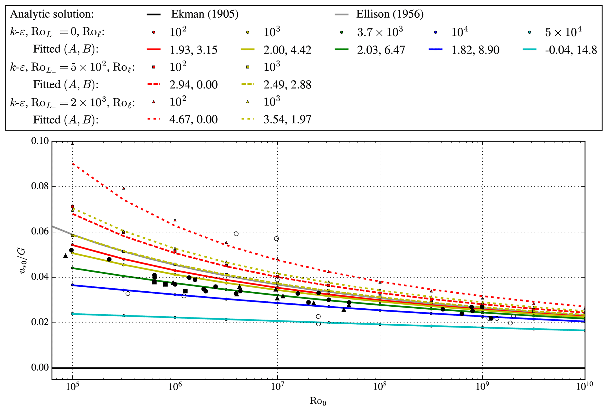
Figure 6 Reproduced from Hess and Garratt (2002). Geostrophic drag coefficient simulated by the limited-length-scale k–ε model extended to unstable surface layer stratification, taken at a normalized height of $(z+z_{\mathrm{0}})\left|f_{\mathrm{c}}\right|/G=\mathrm{5}\times {\mathrm{10}}^{-\mathrm{5}}$ (i.e., in the surface layer), for different Ro₀, Ro_ℓ, and $R{o}_{L_{-}}$. Black markers represent measurements from Hess and Garratt (2002). $R{o}_{\mathrm{\ell }}=\mathrm{3.7}\times {\mathrm{10}}^{\mathrm{3}}$ represents ℓ_max from Blackadar (1962). Analytic results of Ekman (1905) and Ellison (1956) are summarized in Appendix A.

Figure 6 is a reproduction from Hess and Garratt (2002), where the geostrophic drag coefficient is depicted as a function of surface Rossby number Ro₀. The black markers are measurements summarized by Hess and Garratt (2002), where the dots are near-neutral and near-barotropic conditions, the triangles and squares reflect less idealized atmospheric conditions, and the open circles are measurements with a relative high uncertainty. Results of the limited-length-scale k–ε model including the extension to unstable surface layer stratification are shown as colored markers, where the colors represent a range of Ro_ℓ. For the two smallest values of Ro_ℓ, two additional results are plotted for $R{o}_{L_{-}}=\mathrm{5}\times {\mathrm{10}}^{\mathrm{2}}$ and $R{o}_{L_{-}}=\mathrm{2}\times {\mathrm{10}}^{\mathrm{3}}$, representing unstable ($-\mathrm{1}/L=\mathrm{0.005}$ m⁻¹) and very unstable conditions ($-\mathrm{1}/L=\mathrm{0.02}$ m⁻¹) for the chosen values of G=10 m s⁻¹ and $f_{\mathrm{c}}={\mathrm{10}}^{-\mathrm{4}}$ s⁻¹. The colored lines are fitted A and B constants from the GDL as defined in Eq. (28). The analytic solutions from Ekman (1905) and Ellison (1956), as summarized in Appendix A, are shown as black and gray lines, respectively. For $R{o}_{L_{-}}=\mathrm{0}$, the geostrophic drag coefficient predicted by the limited-length-scale k–ε model is bounded by the analytic solutions. For Ro_ℓ→0, the geostrophic drag coefficient of Ellison (1956) is approximated. For increasing Ro_ℓ or decreasing ABL depths, the $\mathit{\{}{u}_{*}\mathrm{0}/G$, log (Ro₀)} relationship becomes more linear. In addition, for $R{o}_{\mathrm{\ell }}=\mathrm{3.7}\times {\mathrm{10}}^{\mathrm{3}}$, as used by Blackadar (1962), and $R{o}_{L_{-}}=\mathrm{0}$, most of the near-neutral and near-barotropic measurements are captured quite well. Hess and Garratt (2002) used the measurements of the geostrophic drag coefficient to validate a number of models, which often have only one result for each Ro₀. The geostrophic drag coefficients predicted by the limited-length-scale k–ε model can cover all measurements by varying Ro_ℓ. In addition, the extension to unstable surface layer conditions can also explain the trend of the more uncertain measurements (black dots). Since Ro_ℓ and $R{o}_{L_{-}}$ influence the ABL depth, as previously shown in Fig. 5, the model suggests that the measurements were conducted for a range of ABL depths that could reflect a range of atmospheric stabilities, although the geostrophic wind shear can play a role here as shown by Floors et al. (2015).

The fitted A and B parameters in Fig. 6 are dependent on Ro_ℓ and $R{o}_{L_{-}}$, which both influence the ABL depth. This is not a surprising result, since many authors have shown that A and B are dependent on atmospheric stability (see, for example, Arya, 1975; Zilitinkevich, 1989; Landberg, 1994). For moderate roughness lengths over land, the measured values tabulated by Hess and Garratt (2002) generally fall between the blue and yellow lines for neutral conditions, which are consistent with the typically used values in wind energy, i.e., A=1.8 and B=4.5 (e.g., Troen and Petersen, 1989). Assuming ℓ_max is a measure of the ABL depth, then in the actual atmosphere over land we have $R{o}_{\mathrm{0}}/R{o}_{\mathrm{\ell }}\sim {\mathrm{10}}^{\mathrm{3}}$–10⁵, while over sea the ratio is roughly 10⁶–10⁷. Thus one can see that the typical wind energy values of A and B are a compromise for applicability over both land and sea. The real-world limits mean that the result for Ro_ℓ=10² (red line) can extend only from Ro₀∼10⁵–10⁷, while the over-sea regime (large Ro₀) tends to involve a smaller range of Ro_ℓ. We note that the GDL from Eq. (27) limits how large B can be; generally $u_{*\mathrm{0}}/G<\mathit{\kappa }/B$, so values of B greater than those shown are not physical. The model results in Fig. 6 do not violate this limit.

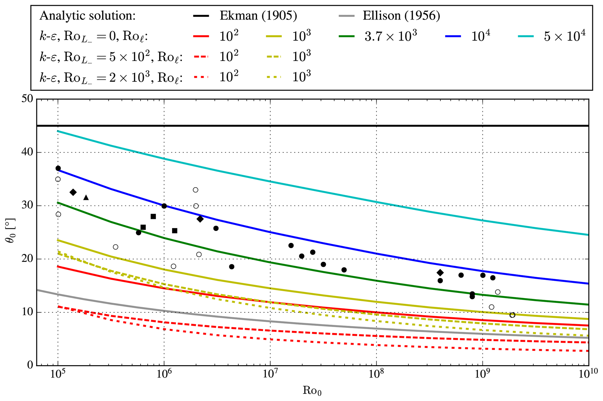
Figure 7 Reproduced from Hess and Garratt (2002). Cross-isobar angle simulated by the limited-length-scale k–ε model extended to unstable surface layer stratification, taken at a normalized height of $(z+z_{\mathrm{0}})\left|f_{\mathrm{c}}\right|/G=\mathrm{5}\times {\mathrm{10}}^{-\mathrm{5}}$ for different Ro₀, Ro_ℓ, and $R{o}_{L_{-}}$. Black markers represent measurements from Hess and Garratt (2002). Ro_ℓ=3.7 represents ℓ_max from Blackadar (1962). Analytic results of Ekman (1905) and Ellison (1956) are summarized in Appendix A.

6.2 Cross-isobar angle

Figure 7 is a reproduction of Hess and Garratt (2002), where the angle between surface wind direction and the geostrophic wind direction is plotted as a function of the surface Rossby number. This angle is known as the cross-isobar angle, θ₀. The black markers, analytic solutions, and model results follow the same definition as used in Fig. 6, where additional black diamond markers are added that correspond to climatological measurements, as discussed by Hess and Garratt (2002). For $R{o}_{L_{-}}=\mathrm{0}$, the model results of the cross-isobar angle are bounded by the analytic solutions, as also found for the geostrophic drag coefficient in Fig. 6. All measurements summarized by Hess and Garratt (2002) can be simulated by the limited-length-scale k–ε model by varying the ABL depth using Ro_ℓ. Most of the measurements are well predicted for $R{o}_{L_{-}}=\mathrm{0}$ and Ro_ℓ=10³–10⁴, which is the range used by Blackadar (1962) ($R{o}_{\mathrm{\ell }}=\mathrm{3.7}\times {\mathrm{10}}^{\mathrm{3}}$). For $R{o}_{L_{-}}\ne \mathrm{0}$, smaller values of the cross-isobar angle can be simulated compared with the analytic solution of Ellison (1956) due to the enhanced rate of mixing. The model cannot predict larger values of the cross-isobar angle compared to the analytic solution of Ekman (1905) (45^∘).

6.3 Atmospheric surface layer profiles

Peña et al. (2014) used measurements of the wind speed components from 10 to 160 m, from The National Test Station for Wind Turbines at Høvsøre, a coastal site in Denmark, characterized as flat grassland. The Coriolis parameter for the test location is $\mathrm{1.21}\times {\mathrm{10}}^{-\mathrm{4}}$ s⁻¹. The measurements were taken from sonic anemometers over 1 year, and a wind direction sector was selected to avoid the influence of the coastline and wind turbine wakes. Peña et al. (2014) also calculated a “mixing” (turbulence) length scale $\widehat{\mathrm{\ell }}$ using a local friction velocity u_* and the wind speed gradient:

$$\begin{array}{}\text{(29)}& \widehat{\mathrm{\ell }}={\displaystyle \frac{u_{*}}{\mathrm{d}U/\mathrm{d}z}}.\end{array}$$

Seven cases were defined based on the atmospheric stability, and these are listed in Table 2 in terms of the Obukhov length, roughness length, and friction velocity. In order to apply the limited-length scale k–ε, we need to set the geostrophic wind speed and the maximum turbulence length scale, which are both unknown. We choose to use G and ℓ_max as free parameters, which we fit to a reference wind speed and a turbulence length scale, at a reference height of 60 m. The wind speed gradient is obtained from a central-difference scheme taking the wind speed at 40, 60, and 80 m. The fitted parameters are obtained by running the numerical simulations with a gradients-based optimizer, and the results are listed in Table 2. The maximum ℓ_max is set to 10³ m, which corresponds to an ABL depth on the order of 5 km, as depicted in Fig. 5. The unstable cases are also simulated with the extended limited-length-scale k–ε model using the measured L and refitted G and ℓ_max, which are listed in Table 2 as values in parentheses.

Table 2 ASL validation cases. Fitted G, fitted ℓ_max, and modeled u_*0 in parentheses represent values for the extended model.

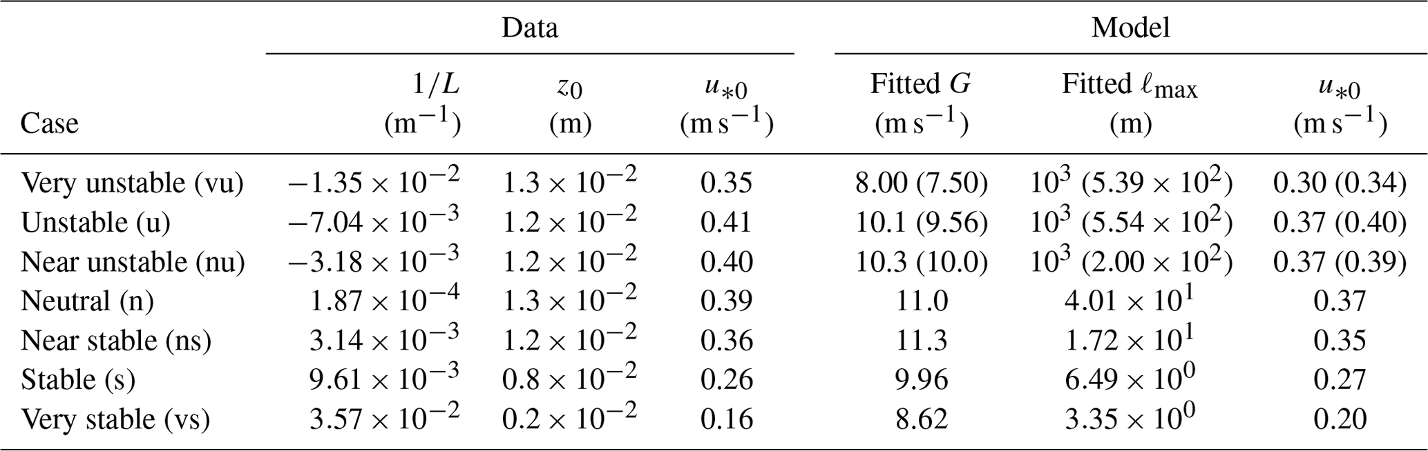
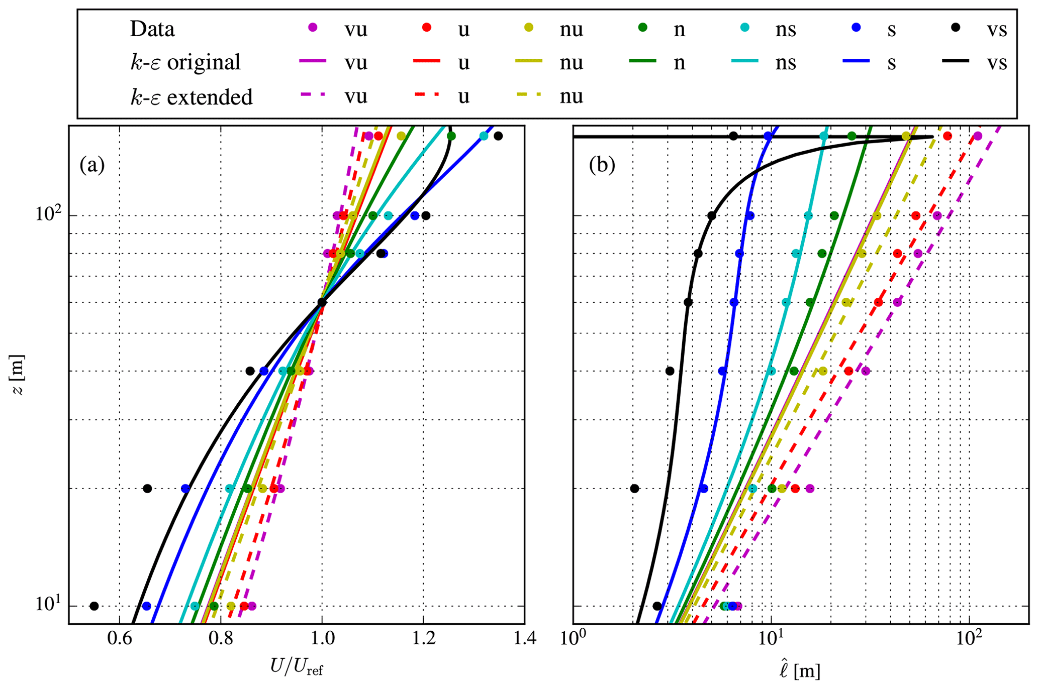
Figure 8 ASL measurements of Peña et al. (2010) compared to simulation results of the original limited-length-scale k–ε model of Apsley and Castro (1997). (a) Wind speed. (b) Turbulence length scale from Eq. (29). Unstable cases are also simulated with our extension to unstable surface layer stratification with L from Table 2.

Figure 8 depicts the wind speed and turbulence length scale of the measurements and numerical simulations using the original and extended limited-length-scale k–ε models. The turbulence length scale from the numerical simulation is calculated by Eq. (29), instead of the usual definition $\mathrm{\ell }=C_{\mathit{\mu }}^{\mathrm{3}/\mathrm{4}}{k}^{\mathrm{3}/\mathrm{2}}/\mathit{\epsilon }$. The original limited-length-scale k–ε model of Apsley and Castro (1997) can capture the wind speed and turbulence length scale for the stable and neutral cases. Note that for the very stable case, the shear is underestimated and the model predicts an ABL depth of about 100 m, which results in a spike in $\widehat{\mathrm{\ell }}$, since dU∕dz is zero around the ABL depth. As expected, the original limited-length-scale k–ε model cannot predict a lower shear and a larger turbulence length scale compared to neutral atmospheric conditions (where $\mathrm{d}U/\mathrm{d}z=u_{*}/\mathrm{\ell }$ and ℓ=κz), and the optimizer used to fit G and ℓ_max sets ℓ_max to our chosen maximum value of 10³ m. Note that therefore the lines corresponding to unstable conditions of the original k–ε model largely overlap in Fig. 8. Higher values of ℓ_max would not improve the results. The limited-length-scale k–ε model extended to unstable surface layer stratification is able to predict turbulence length scales larger than ℓ=κz and shows improved results for both the shear and the turbulence length scale.

Table 2 also shows the measured and simulated friction velocity at a height of 10 m. The simulated friction velocity is calculated as $u_{*}=({\stackrel{\mathrm{‾}}{u^{\prime }{w}^{\prime }}}^{\mathrm{2}}+{\stackrel{\mathrm{‾}}{v^{\prime }{w}^{\prime }}}^{\mathrm{2}}{)}^{\mathrm{1}/\mathrm{4}}$. For the unstable cases, it is clear that the extended model predicts friction velocities that are closer to the measurements compared to the original limited-length-scale k-ε model due to the enhanced mixing.

It should be noted that the validation presented in Fig. 8 could be considered as a best-possible simulation-to-measurement comparison because we have allowed ourselves to tune both G and ℓ_max. When G is provided by the measurements, it is more difficult to obtain a good match, as shown in Sect. 6.4.

Table 3 ABL validation cases based on Peña et al. (2014).

6.4 Atmospheric-boundary-layer profiles

Peña et al. (2014) performed lidar measurements of the horizontal wind speed components from 10 to 1200 m at the same test site as discussed in Sect. 6.3. Peña et al. (2014) selected 10 cases that differ in geostrophic forcing and atmospheric stability. The cases were selected to challenge the validation of numerical models. Since our numerical setup can only handle a constant geostrophic wind speed, we select the barotropic cases from Peña et al. (2014): cases 4, 5, and 9 and the corresponding values of the Obukhov length, geostrophic wind, roughness length, friction velocity, Ro₀, and $R{o}_{L_{-}}$ are listed in Table 3. For convenience, we keep the case names as introduced by Peña et al. (2014). Cases 4 and 5 represent a stable and a neutral ABL with high forcing, respectively, where Ro₀=10⁷. Case 9 is characterized by a low forcing and very unstable stratification, where $R{o}_{\mathrm{0}}=\mathrm{2.8}\times {\mathrm{10}}^{\mathrm{6}}$.

In Case 6 from Peña et al. (2014) it is observed that the lidar measurements do not approach the geostrophic wind speed at large heights above the surface. This is because the geostrophic wind speed in Peña et al. (2014) is derived from outputs of the Weather Research and Forecasting (WRF) model over a large area, potentially leading to bias. Therefore, we use a slightly different approach to estimate the geostrophic wind; because the wind speed above the ABL is nearly always in geostrophic balance we can just assume the wind speed measured by the wind lidar above the boundary layer depth to be equal to the geostrophic wind speed, thereby avoiding possible prediction errors in wind speed from the WRF model. Instead, only the ABL depth is estimated from the WRF model outputs. The ABL depth is available as a diagnostic variable predicted by the Yonsei University ABL scheme (Hong et al., 2006) in the WRF model. To be sure that the lidar wind speed is close to the geostrophic wind speed, we always estimate it from the level that is higher than the modeled ABL depth during all 30 min means, which constitute the three cases.

Since G is known, we can use Rossby similarity for model validation. While one could try to find an ℓ_max to get the best comparison with the measurements, we find that it is difficult to define a good metric. For example, we could attempt to find an ℓ_max that results in an equivalent ABL depth equal to that of the measurement cases; however, the ABL depth was not directly measured and only estimated from a model. Instead of finding a single ℓ_max value, we choose to simulate a range of ℓ_max values. We note that part of this difficulty is due to the limited extent of the model. There is no “top-down” information; i.e., we lack entrainment effects and the impact of the strength of the capping inversion. An extra length scale could be introduced to account for such effects; examples are the nonlocal static stability scale found in Zilitinkevich and Esau (2005), the “mid-ABL” scale of Gryning et al. (2007) (generalized by Kelly and Troen (2016) for matching G), and the “top-down” scale of Kelly et al. (2019).

Figure 9 depicts the measured wind speed and wind direction, for each validation case. Since cases 4 and 5 have the same G (within 5 %) and thus same surface Rossby number Ro₀≃10⁷, we can plot them together because the normalized model results are the same for both cases. The error bars represent the standard error of the mean. The original limited-length-scale k–ε model of Apsley and Castro (1997) is employed with a range of Ro_ℓ. The unstable ABL case (Case 9) is also simulated with the model extension to unstable surface layer stratification using $R{o}_{L_{-}}$ from Table 3 and the two smallest values of Ro_ℓ. Case 4 has a strong wind shear and a wind veer that leads to a cross-isobar angle of 50^∘. The limited-length-scale k–ε model can predict a maximum cross-isobar angle of 45^∘ for extremely shallow ABL depths, as shown in Sect. 6.2. Hence, the measured ABL from Case 4 is not a possible numerical solution. The measured ABL from Case 5 can be predicted by the original limited-length-scale k–ε model, while this is not the case for the wind speed close to the ground of Case 9 due to the strong unstable stratification. When the limited-length-scale k–ε model including the extension for unstable surface layer conditions is employed, the prediction of the wind speed near the ground is improved, although it is difficult to correctly predict both wind speed and wind direction. It should be noted that the extended (unstable) model only improves the wind speed in the surface layer (at 10 m), noting the dotted and solid lines crossing in Fig. 9c.

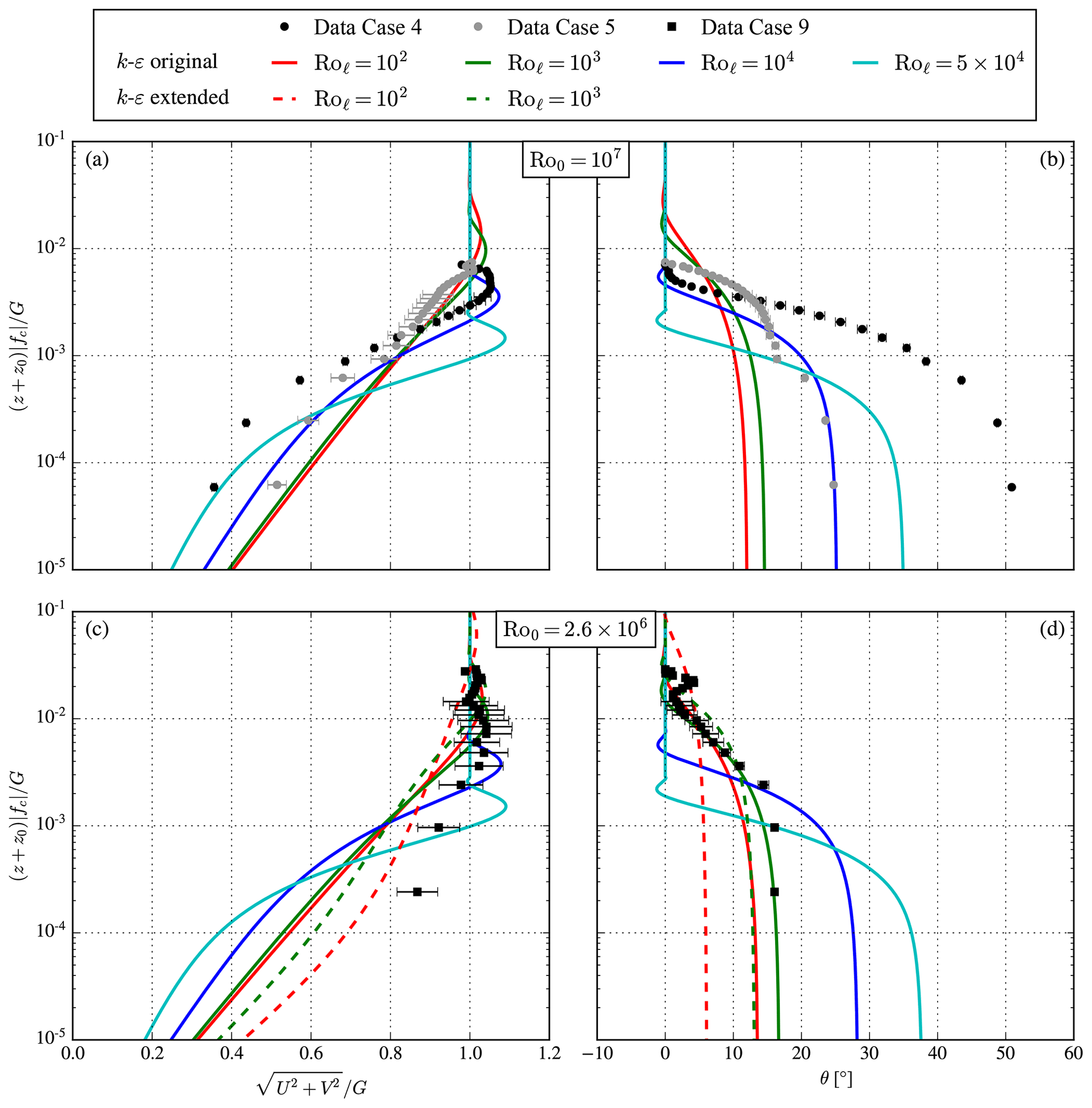
Figure 9 ABL measurements from Peña et al. (2014) compared to simulation results of the original limited-length-scale k–ε model of Apsley and Castro (1997), for a range of Ro_ℓ. (a, c) Wind speed. (b, d) Wind direction. Unstable Case 9 (c, d) is also simulated with our extension to unstable surface layer stratification (dashed lines), with $R{o}_{L_{-}}$ (i.e., 1∕L) from Table 3.

From the measurements during Case 9 it was observed that the WRF-modeled ABL depth grew from 300 m to nearly 1200 m, which indicates that the conditions were largely transient; such nonstationary conditions are difficult for a RANS model. More unstable cases are necessary to further validate the extended model, including measurements of turbulence quantities such as the (total) turbulence intensity. It is possible to use validation cases based on turbulence-resolving methods, such as large-eddy simulations, in future work.

7 Conclusions

The idealized ABL was simulated with a one-dimensional RANS solver, using two different turbulence closures: a limited mixing-length model and a limited-length-scale k–ε model. While these models require four input parameters, we have shown that the simulated ABL profiles collapse to a dependence upon two Rossby numbers, which are defined by the roughness length and the maximum turbulence length scale, respectively. The Rossby number based on the maximum turbulence length scale is a new dimensionless number and is related to the ABL depth. The model-based Rossby number similarity obtained herein is valid for both turbulence models. We have employed Rossby number similarity to compare the range of model solutions with historical measurements of relevant associated meteorological quantities, such as the geostrophic drag coefficient and cross-isobar angle. The measured variation in these measurements can be explained by dependence upon the new Rossby number (i.e., ABL depth). In addition, we have shown how two classic analytic solutions of the idealized ABL (Ekman, 1905; Ellison, 1956) act as bounds on the results obtainable by the limited-length-scale k–ε model.

The limited-length-scale turbulence closures can represent the effects of stable and neutral stratification but cannot model unstable conditions. We have proposed simple extensions to overcome this issue, without adding a temperature equation (van der Laan et al., 2017). The extended models require an additional input, the Obukhov length, which can be used to define a third Rossby number. We have shown that the extension of the k–ε model compares well with measurements of seven ASL profiles, representing a range of atmospheric stabilities, including three unstable cases. The k–ε model further offers turbulence intensity, whose profile is also found to collapse according to the developed similarity theories. A model validation of the ABL for a stable, a neutral, and an unstable case is performed, with less success for the non-neutral cases. In the very stable case, the measured wind veer of 50^∘ was larger than the maximum wind veer of 45^∘ that the k–ε model can simulate. In addition, the very unstable case was characterized by nonstationary conditions, which are difficult to capture with a RANS model. More validation cases based on the convective ABL are necessary to quantify the performance of the turbulence model extension to unstable conditions beyond the surface layer.

The application of the one-dimensional RANS simulations to generate inflow profiles for three-dimensional RANS simulations is not performed here and it should be investigated in future work. Ongoing and future work also includes the incorporation of the effect of the capping-inversion strength to accommodate entrainment at the ABL top (softening the ABL lid, one might say); this can be considered as an introduction of an additional length scale. In addition, the effects of length-scale limitation and neglecting the buoyancy force in the momentum equation need to be quantified for three-dimensional RANS simulations of complex terrain and wind farms.

Appendix A: Analytic solutions for the idealized ABL

A1 Constant eddy viscosity – Ekman spiral

The analytic solution of Ekman (1905), known as the Ekman spiral, can be expressed as a function of a single variable, the normalized height $\mathit{\xi }\equiv z\sqrt{\left|f_{\mathrm{c}}\right|/\left(\mathrm{2}{\mathit{\nu }}_T\right)}$. The wind speed $S=\sqrt{U^{\mathrm{2}}+V^{\mathrm{2}}}$ and the wind direction θ can be written as

$$\begin{array}{}\text{(A1)}& {\displaystyle }\begin{array}{rl}& S\left(\mathit{\xi }\right)=G\sqrt{\mathrm{1}-\mathrm{2}\cos \left(\mathit{\xi }\right)\exp (-\mathit{\xi })+\exp (-\mathrm{2}\mathit{\xi })},\\ & \mathit{\theta }\left(\mathit{\xi }\right)=\arctan \left({\displaystyle \frac{\sin \left(\mathit{\xi }\right)}{\exp \left(\mathit{\xi }\right)-\cos \left(\mathit{\xi }\right)}}\right).\end{array}\end{array}$$

The cross-isobar angle θ(0) is found to be 45^∘, and the geostrophic drag coefficient is zero (since there is no roughness or u_* within Ekman theory).

A2 Linear eddy viscosity – Ellison

The analytic solution of Ellison (1956) for the U and V velocity components can be written in terms of the Kelvin functions ker and kei, as discussed by Krishna (1980):

$$\begin{array}{}\text{(A2)}& U=cG\text{ker}\left(x\right)+U_{\mathrm{G}},V=cG\text{kei}\left(x\right)+V_{\mathrm{G}},\end{array}$$

where x is a normalized height $x\equiv \mathrm{2}\sqrt{z\left|f_{\mathrm{c}}\right|/\left(\mathit{\kappa }{u}_{*\mathrm{0}}\right)}$ and c is a constant. For z→z₀ (and assuming $z_{\mathrm{0}}\ll u_{*\mathrm{0}}/\left|f_c\right|$), the Kelvin functions can be expanded, and the solution can be written as

$$\begin{array}{}\text{(A3)}& \begin{array}{rl}& U\approx -cG\left[{\displaystyle \frac{\mathrm{1}}{\mathrm{2}}}\ln \left({\displaystyle \frac{z_{\mathrm{0}}\left|f_{\mathrm{c}}\right|}{\mathit{\kappa }{u}_{*\mathrm{0}}}}\right)+{\mathit{\gamma }}_{\mathrm{e}}\right]+U_{\mathrm{G}}=\mathrm{0},\\ & V\approx -cG{\displaystyle \frac{\mathit{\pi }}{\mathrm{4}}}+V_{\mathrm{G}}=\mathrm{0},\end{array}\end{array}$$

where γ_e≈0.57721 is the Euler–Mascheroni constant. We can set the geostrophic wind G through the constant c:

$$\begin{array}{}\text{(A4)}& \begin{array}{rl}& c=-{\left({\left[{\displaystyle \frac{\mathrm{1}}{\mathrm{2}}}\ln \left({\displaystyle \frac{z_{\mathrm{0}}\left|f_{\mathrm{c}}\right|}{\mathit{\kappa }{u}_{*\mathrm{0}}}}\right)+{\mathit{\gamma }}_{\mathrm{e}}\right]}^{\mathrm{2}}+{\displaystyle \frac{{\mathit{\pi }}^{\mathrm{2}}}{\mathrm{16}}}\right)}^{-\mathrm{1}/\mathrm{2}},\\ & U_{\mathrm{G}}=cG\left[{\displaystyle \frac{\mathrm{1}}{\mathrm{2}}}\ln \left({\displaystyle \frac{z_{\mathrm{0}}\left|f_{\mathrm{c}}\right|}{\mathit{\kappa }{u}_{*\mathrm{0}}}}\right)+{\mathit{\gamma }}_{\mathrm{e}}\right],V_{\mathrm{G}}=cG{\displaystyle \frac{\mathit{\pi }}{\mathrm{4}}}.\end{array}\end{array}$$

Note that Krishna (1980) chose $cG=-\mathrm{2}{u}_{*\mathrm{0}}/\mathit{\kappa }$ (so his −c is 5 times the geostrophic drag coefficient $u_{*\mathrm{0}}/G$ for κ=0.4), which follows from the Neumann condition,

$$\begin{array}{}\text{(A5)}& {\displaystyle \frac{\mathrm{d}U}{\mathrm{d}z}}={\displaystyle \frac{u_{*\mathrm{0}}}{\mathit{\kappa }z}}=-{\displaystyle \frac{cG}{\mathrm{2}z}},\end{array}$$

by taking dU∕dz in Eq. (A2) for z→z₀. As as consequence, the geostrophic wind becomes a dependent parameter. We prefer to keep the geostrophic wind as an independent parameter by using c as defined in Eq. (A4). Then, the effective u_*0 is calculated as $u_{*\mathrm{0},\mathrm{eff}}=cG\mathit{\kappa }/\mathrm{2}$.

A GDL can be derived in the form of Eq. (28) by using the Neumann conditions of Eq. (A5) and the constant c from Eq. (A4), where $A=-\ln \left(\mathit{\kappa }\right)+\mathrm{2}{\mathit{\gamma }}_{\mathrm{e}}\approx \mathrm{2.07}$ and $B=\mathit{\pi }/\mathrm{2}\approx \mathrm{1.57}$, as also shown by Krishna (1980). The friction velocity in Eq. (A4) can now be calculated by solving the GDL for $u_{*\mathrm{0}}/G$. Hence, the analytic solution of Ellison (1956) is only dependent on Ro₀.

The cross-isobar angle (angle between the geostrophic wind direction and surface wind direction) can be written as a function of the geostrophic drag coefficient $u_{*\mathrm{0}}/G$ and the Rossby number Ro₀ using Eq. (A4):

$$\begin{array}{}\text{(A6)}& {\mathit{\theta }}_{\mathrm{0}}=\arctan \left({\displaystyle \frac{V_{\mathrm{G}}}{U_{\mathrm{G}}}}\right)=\arctan \left({\displaystyle \frac{\mathit{\pi }/\mathrm{2}}{\mathrm{2}{\mathit{\gamma }}_{\mathrm{e}}-\ln \left(R{o}_{\mathrm{0}}\right)-\ln \left(\mathit{\kappa }{u}_{*\mathrm{0}}/G\right)}}\right),\end{array}$$

where the GDL can be used to solve for $u_{*\mathrm{0}}/G$.

Appendix B: Rossby number similarity based on the friction velocity

In this article, we have shown a Rossby similarity of two limited-length-scale turbulence closures using the geostrophic wind speed, G, as a velocity scale, instead of the friction velocity near the ground, u_0*. It is more convenient to use G because it is a constant and a model input, while u_0* is a model result that depends on height. However, it is possible to obtain a Rossby similarity based on u_0* using the geostrophic drag coefficient $u_{*\mathrm{0}}/G$ from Fig. 6, since we can write the following:

$$\begin{array}{}\text{(B1)}& \begin{array}{rl}& R{o}_{\mathrm{\ell }}^{*}\equiv {\displaystyle \frac{u_{*\mathrm{0}}}{\left|f_{\mathrm{c}}\right|{\mathrm{\ell }}_{\max }}}={\displaystyle \frac{u_{*\mathrm{0}}}{G}}R{o}_{\mathrm{\ell }},\\ & R{o}_{\mathrm{0}}^{*}\equiv {\displaystyle \frac{u_{*\mathrm{0}}}{\left|f_{\mathrm{c}}\right|z_{\mathrm{0}}}}={\displaystyle \frac{u_{*\mathrm{0}}}{G}}R{o}_{\mathrm{0}},\\ & R{o}_{L_{-}}^{*}\equiv {\displaystyle \frac{-u_{*\mathrm{0}}}{\left|f_{\mathrm{c}}\right|L}}={\displaystyle \frac{u_{*\mathrm{0}}}{G}}R{o}_{L_{-}}.\end{array}\end{array}$$

Figure 6 can be transformed into an explicit relation of $u_{*\mathrm{0}}/G$ as a function of $R{o}_{\mathrm{\ell }}^{*}$, $R{o}_{\mathrm{0}}^{*}$, and $R{o}_{L_{-}}$; the result is depicted in Fig. B1 for $R{o}_{L_{-}}^{*}=\mathrm{0}$.

The Rossby similarity based on u_0* is illustrated in Fig. B2 for four combinations of $R{o}_{\mathrm{0}}^{*}$ (10⁵ and 10⁸) and $R{o}_{\mathrm{\ell }}^{*}$ (10² and 10⁴) for $R{o}_{L_{-}}=\mathrm{0}$, using four combinations of u_*0 (0.2 and 0.4 m s⁻¹) and f_c ($\mathrm{5}\times {\mathrm{10}}^{-\mathrm{5}}$ and 10⁻⁴ s⁻¹). Only results of the limited-length-scale k–ε model are shown for brevity, although the Rossby similarity based on u_0* also applies to the limited mixing-length model and for the unstable extension (where $R{o}_{L_{-}}\ne \mathrm{0}$).

It should be noted that u_0* in Fig. 6 was extracted at a normalized height of $(z+z_{\mathrm{0}})\left|f_{\mathrm{c}}\right|/G=\mathrm{5}\times {\mathrm{10}}^{-\mathrm{5}}$, which represents the surface layer. If a perfect Rossby similarity based on u_0* is desired, one would need to extract u_0* at a constant normalized height equal to $(z+z_{\mathrm{0}})\left|f_{\mathrm{c}}\right|/u_{\mathrm{0}*}$, which requires an iterative process of finding a geostrophic wind speed that results in a RANS simulation with a desired u_0*, at a constant normalized height. This is beyond the scope of the present work.

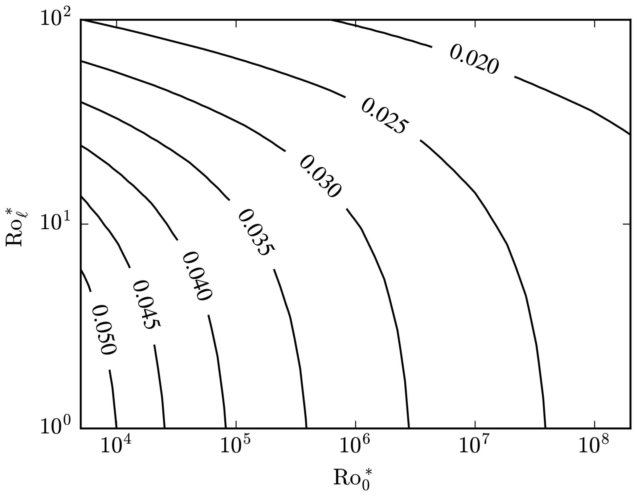
Figure B1 Geostrophic drag coefficient simulated by the limited-length-scale k-ε model as a function of $R{o}_{\mathrm{\ell }}^{*}$ and $R{o}_{\mathrm{0}}^{*}$ with $R{o}_{L_{-}}^{*}=\mathrm{0}$.

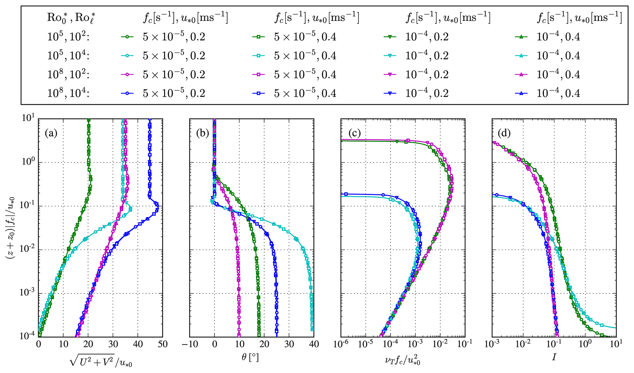
Figure B2 Rossby number similarity of the limited-length-scale k–ε model using the friction velocity as the velocity scale, for $R{o}_{L_{-}}=\mathrm{0}$.