Beamlike models for the analyses of curved, twisted and tapered horizontal-axis wind turbine (HAWT) blades undergoing large displacements

Continuous ongoing efforts to better predict the mechanical behaviour of complex beamlike structures, such as wind turbine blades, are motivated by the need to improve their performance and reduce the costs. However, new design approaches and the increasing flexibility of such structures make their aeroelastic modelling ever more challenging. For the structural part of this modelling, the best compromise between computational efficiency and accuracy can be obtained via schematizations based on suitable beamlike elements. This paper addresses the modelling of the mechanical behaviour of beamlike structures which are curved, twisted and tapered in their unstressed state and undergo large displacements, in- and out-of-plane cross-sectional warping, and small strains. A suitable model for the problem at hand is proposed. Analytical and numerical results obtained by its application are presented and compared with results from 3D FEM analyses.

1 Introduction

New methods are continuously being sought to improve the performance and efficiency of horizontal-axis wind turbines (HAWTs). Specifically, such improvements aim to increase their energy capture capacity, develop more reliable structures and lower overall energy costs (Wiser et al., 2016). Such goals can be achieved through the use of advanced materials, the optimization of the aerodynamic and structural behaviour of the blades, and the exploitation of load control techniques (see, for example, Ashwill et al., 2010; Bottasso, 2012; Stäblein, 2017). However, new design strategies and the increasing flexibility of those structures make modelling their aeroelastic behaviour ever more challenging. For the structural part of this modelling, schematizing the blades through suitable beamlike elements may represent the best compromise between computational efficiency and accuracy. Modern blades are however very complex beamlike structures. They may be curved, twisted and also tapered in their unstressed state. Even ignoring the complexities related to the materials and loading conditions, their shape alone is sufficient to make mathematical description of their mechanical behaviour a very challenging task. This work addresses the modelling of the mechanical behaviour of structures of this kind, with a particular focus on their main geometrical characteristics, such as the twist and taper of the transversal cross sections, as well as the in- and out-of-plane cross-sectional warping and the large deflections of their reference centre line.

Over the years several theories have been developed for beamlike structures (see, for example, Love, 1944; Antman, 1966; Rubin, 2000) for applications in different fields, from helicopter rotor blades in aerospace engineering to bridge components in civil engineering and surgical tools in medicine. Nevertheless, due to the continuous need for ever more rigorous and application-oriented models, interest in advanced theories for complex beamlike structures has led to even further research in recent years. The focus of this paper is on the effects of important geometrical characteristics of those structures, such as the curvature of their centre line as well as the twist and the taper of their cross sections. After an introduction to modelling approaches for structures of this kind (Sect. 2), a suitable model is proposed for the problem at hand (Sect. 3). Finally, analytical results and numerical examples obtained by applying the proposed modelling approach to reference beamlike structures are presented and compared with results from 3D FEM analyses (Sects. 4 and 5).

2 Overview of modelling approaches

Modelling the mechanical behaviour of modern blades can be performed via different approaches. See, for example, the reviews on aeroelastic modelling approaches for wind turbine blades of Hansen et al. (2006) and L. Wang et al. (2016), which discuss and compare aerodynamic and structural models used in research and industrial applications. For the structural modelling, two main choices are based on 3D FEM and beam models. In general, 3D FEM approaches can be very accurate and flexible, but they can be computationally demanding for analyses of complex systems, especially if they are coupled with CFD methods for aerodynamic analyses. The overall computational cost can be reduced using faster aerodynamic models, such as those based on the blade element momentum theory (see, for example, Hansen et al., 2006). However, this may not yet be sufficient in the case of multi-objective optimization tasks, in which the optimization of several aspects (e.g. aerodynamic performance, structural characteristics and control systems) has to be addressed at the same time (see also Bottasso et al., 2012). Therefore, faster structural models may be needed as well, such as suitable beam models, which may provide accurate information on the deflection of the structure's centre line as well as the strain and stress fields in the three-dimensional solid. The use of fast aerodynamic models along with suitable beam models may then represent the best compromise between computational efficiency and accuracy. In this work, the focus is only on the structural modelling. In particular, a mathematical model is proposed to simulate the behaviour of non-prismatic beamlike structures, which may be curved, twisted and tapered in their unstressed reference state and undergo large deflections, in- and out-of-plane cross-sectional warping, and small strains (such a model is referred to here as a beamlike model or BLM).

Over the years many approaches have been developed for beamlike structures, from classical beam models (Love, 1944) for extension, twisting and bending to the formulation of Reissner (1981), which also accounts for transverse shear deformation, to geometrically exact and asymptotic approaches, involving the research efforts of many investigators (such as Antman, 1966; Giavotto et al., 1983; Simo, 1985; Ibrahimbegovic, 1995; Ruta et al., 2006; Pai, 2011; Yu et al., 2012; Hodges, 2018). The available theories may be broadly grouped into engineering theories and mathematical ones. The former are usually based on ad hoc corrections to simpler theories (e.g. Rosen and Friemann, 1978) or exploit geometrically exact approaches (such as Q. Wang et al., 2016); the latter are generally based on the directed continuum (see, for example, Rubin, 2000) or exploit asymptotic methods (e.g. Yu et al., 2012). Reviews on beam theories, which summarize modelling approaches and complicating effects, are also available in the literature. For example, many theories have been developed for helicopter rotor blades with an initial twist (Hodges, 1990). In this regard, a wide-ranging review on pre-twisted rods is by Rosen (1991), which covers several aspects of the problem, from the response to static loads to dynamics and stability issues. Kunz (1994) also provided an overview on modelling methods for rotating beams, discussing how engineering theories for rotor blades have evolved over the years, from the recognition of the importance of bending flexibility to the development of linear equations for bending and torsion to the introduction of non-linear terms to such equations. More recently, Rafiee et al. (2017) reviewed the vibrations control issues in rotating beams, summarizing beam theories and complicating effects, such as non-uniform cross sections, initial curvature, twist and sweep. In general, it seems that, unlike for the case of pre-twisted rods, the results published for curved rotating beams with initial taper and sweep are quite scarce, although all these geometrical characteristics may play an important role. This is particularly true for modern wind turbine blades, which are ever more flexible and longer than in the past, pre-bent and swept, and, in addition, characterized by significant chord and twist variations.

To date many research efforts have been devoted to developing powerful theories for beamlike structures. However, complex non-prismatic cases still require further investigation. In general, the geometry of the reference and current states of the structure must be appropriately described, as the curvature, twist and taper are important geometrical design features and should be explicitly included in the model. Moreover, the analysis should not be restricted to small displacements. The model should provide the stress and strain fields in the three-dimensional solid, be rigorous and application-oriented, and provide classical results when applied to prismatic cases. Following these guidelines, a mathematical model to simulate the mechanical behaviour of the mentioned non-prismatic beamlike structures is proposed hereafter.

3 Mechanical model for complex beamlike structures

Here we are concerned with developing a mathematical model to describe the mechanical behaviour of beamlike structures which are curved, twisted and tapered in their reference state and undergo large displacements. One of the main issues with such a task is how to describe the motion of the structure. See, among others, the works of Simo (1985), Ruta et al. (2006) and Pai (2014) for some examples of different approaches. Here, we consider a non-prismatic beamlike structure as a collection of deformable plane figures (i.e. the reference cross sections) along a suitable three-dimensional curve (i.e. the reference centre line). We assume that each point of each cross section in the reference state moves to its position in the current state through a global rigid motion on which a local general (warping) motion is superimposed. In this manner, the cross-sectional deformation can be examined independently of the global motion of the centre line. It is thus possible to consider the global motion to be large, while the local motion and the strain may be small. An analytical description of how the motion of the considered structure is modelled in this work is presented and further discussed in the following section.

3.1 Kinematics and strain measures

We begin by introducing two local triads of orthogonal unit vectors. The first is the local triad, b_i, in the reference state, with b₁ aligned to the tangent vector of the reference centre line. This frame is a function of the reference arch length s; that is b_i=b_i(s). The second local triad, a_i, is a suitable image of the local triad b_i in the current state. This frame is a function of the reference arch length s and time t; that is $a_i=a_i(s,t)$. In general, a₁ is not required to be aligned to the tangent vector of the current centre line. Figure 1 shows a schematic representation of the reference (left) and current (right) states of a beamlike structure. The generic cross section in the reference state is contained in the plane of vectors b₂ and b₃. In the current state, if the cross section remains plane (i.e. unwarped), it can belong to the plane of vectors a₂ and a₃. However, the generic cross section may not remain plane, so we consider that its current (warped) state is attained by superimposing an additional motion to the positions of the points of the unwarped cross section, as in Fig. 1 (right).

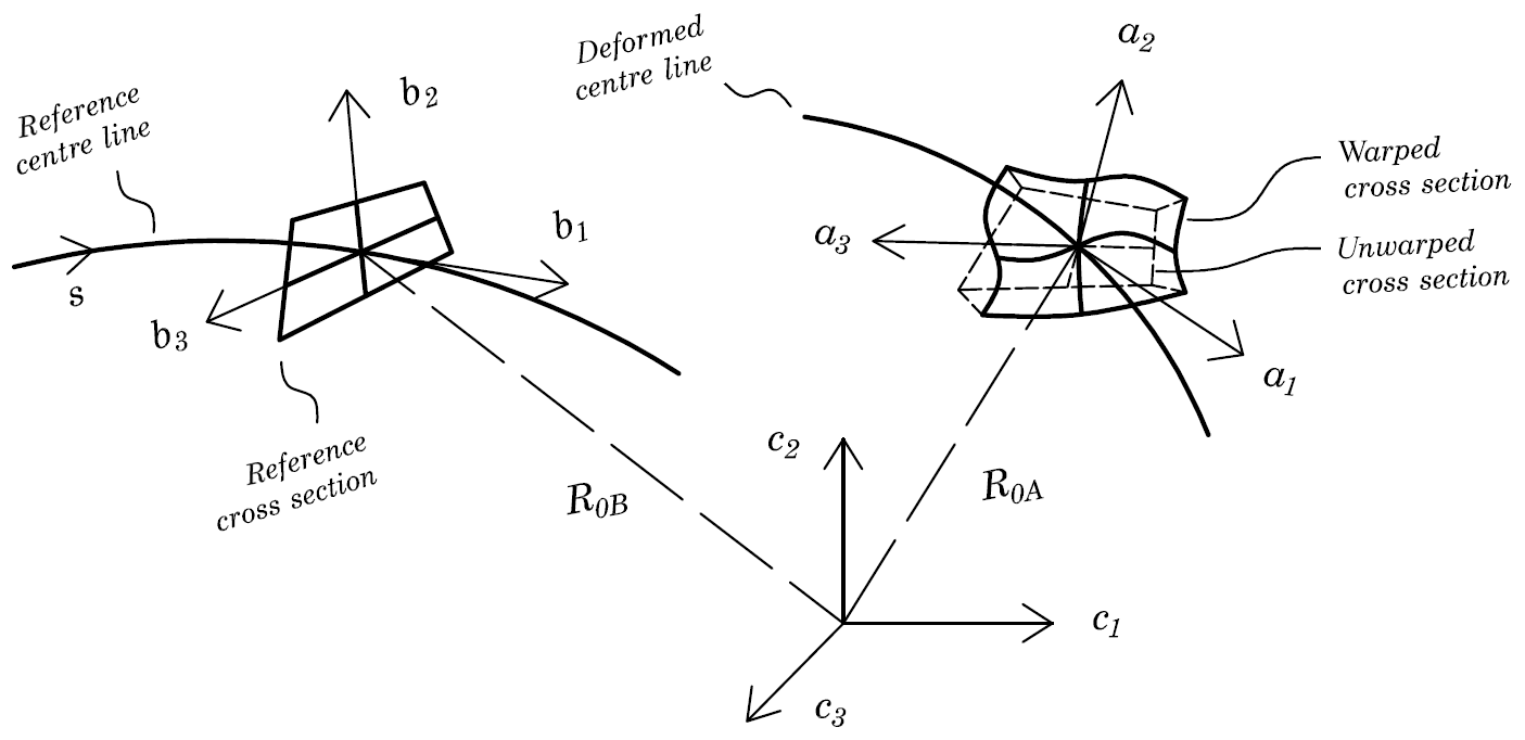
Figure 1 Schematic of the reference and current states, centre lines, cross sections, and local frames.

We continue by introducing the kinematic variables we use to describe the motion of the considered structure. To this end, the orientation of frames a_i and b_i relative to a fixed rectangular frame, c_i, are defined as follows:

$$\begin{array}{}\text{(1)}& a_i=A{c}_i,b_i=B{c}_i,\end{array}$$

where A and B are two proper orthogonal tensor fields (i.e. their determinant is 1; see, for example, Gurtin, 1981). We also introduce a tensor field, T, which defines the relative orientation between frames a_i and b_i as follows:

$$\begin{array}{}\text{(2)}& a_i=T{b}_i=A{B}^T{b}_i.\end{array}$$

We define two skew tensor fields, K_A and K_B, and their axial vectors, k_A and k_B, which are related to the curvatures of the structure's centre line in the current and reference states, as follows (see, for example, Simo, 1985; Gurtin, 1981):

$$\begin{array}{}\text{(3)}& \begin{array}{rl}& K_A=A^{\prime }{A}^T,a_i^{\prime }=K_A{a}_i={\mathit{k}}_A\wedge a_i,\\ & K_B=B^{\prime }{B}^T,b_i^{\prime }=K_B{b}_i={\mathit{k}}_B\wedge b_i,\end{array}\end{array}$$

where the prime denotes derivative with respect to the arch length, s, while the operator ∧ is the usual cross product.

In a similar manner, we introduce the skew tensor field Ω and its axial vector field, ω, related to the variation in vectors, a_i, over time, t, as follows:

$$\begin{array}{}\text{(4)}& \mathrm{\Omega }=\dot{A}{A}^T,{\dot{a}}_i=\mathrm{\Omega }{\mathit{a}}_i=\mathit{\omega }\wedge a_i.\end{array}$$

The dot (over the variables) denotes derivative over time, t. At this point, it is easy to obtain the following identities:

$$\begin{array}{}\text{(5)}& \begin{array}{rl}& T^{\prime }{T}^T=K_A-T{K}_B{T}^T,\dot{T}{T}^T=\mathrm{\Omega },\\ & \mathit{\varphi }\left[T^{\prime }{T}^T\right]=k_A-T{k}_B,\mathit{\varphi }\left[\dot{T}{T}^T\right]=\mathit{\omega },\end{array}\end{array}$$

where the operator ϕ[ ] provides the axial vector of the skew tensor between brackets.

Function R_0B, which maps the points of the centre line in the reference state, does not depend on time, while R_0A can change over time t. Its variation is the time rate of change in the position of the points of the current centre line:

$$\begin{array}{}\text{(6)}& {\dot{R}}_{\mathrm{0}A}=v_{\mathrm{0}}.\end{array}$$

We are now in a position to introduce two important kinematic identities:

$$\begin{array}{}\text{(7)}& \begin{array}{rl}& v_{\mathrm{0}}^{\prime }-\mathit{\omega }\wedge R_{\mathrm{0}A}^{\prime }=T\dot{\mathit{\gamma }},\\ & {\mathit{\omega }}^{\prime }=T\dot{k},\end{array}\end{array}$$

where γ and k are

$$\begin{array}{}\text{(8)}& \begin{array}{rl}& \mathit{\gamma }=T^T{R}_{\mathrm{0}A}^{\prime }-R_{\mathrm{0}B}^{\prime },\\ & k=T^T{k}_A-k_B.\end{array}\end{array}$$

It is worth noting that γ and k vanish for rigid motions and are invariant under superposed rigid motion; hence, they are well-defined measures of strain for beamlike structures (see, for example, Ruta et al., 2006; Rubin, 2000).

Now, we start modelling the motion of the cross section's points. In particular, we introduce two mapping functions, R_A and R_B, to identify the positions of the points of the 3D beamlike structure in its current and reference states. Regarding the reference state, we define the (reference) mapping function as

$$\begin{array}{}\text{(9)}& R_B\left(z_i\right)=R_{\mathrm{0}B}\left(z_{\mathrm{1}}\right)+x_{\mathit{\alpha }}\left(z_i\right){\mathit{b}}_{\mathit{\alpha }}\left(z_{\mathrm{1}}\right),\end{array}$$

where R_0B is the position of the points of the reference centre line relative to frame c_i, b_α is the vectors of the reference local frame in the plane of the reference cross section, x_α identifies the positions of the points in the reference cross section relative to the reference centre line and, finally, z_i is independent mathematical variables which are independent of time. In particular, z₁ is equal to the arch length s, and z_α belongs to a bi-dimensional mathematical domain which is used to map the position of the cross section's points, x_α. Throughout this paper, Greek indices take on values 2 and 3, Latin indices assume values 1, 2 and 3, and repeated indices are summed over their range.

It is worth noting that x_k may or may not be equal to z_k. The former (equality) leads to common modelling approaches available in the literature (see, for example, Simo, 1985; Pai, 2011; Yu et al., 2012). Herein, we choose a set of relations between the position variables x_k and the mathematical variables z_k to provide a description of the shape of the considered beamlike structure, which can be curved, twisted and also tapered in its reference state. In particular, the spanwise variation in the cross section's shape is analytically modelled by means of a mapping of the following type:

$$\begin{array}{}\text{(10)}& x_i={\mathrm{\Lambda }}_{ij}{z}_j,\end{array}$$

where the coefficients Λ_ij are functions of z₁. In the following, we will consider the case of the curved and twisted beamlike structures with bi-tapered cross sections, in which case the map (Eq. 10) reduces to

$$\begin{array}{}\text{(11)}& x_{\mathrm{1}}=z_{\mathrm{1}},x_{\mathrm{2}}=z_{\mathrm{2}}{\mathit{\lambda }}_{\mathrm{2}}\left(z_{\mathrm{1}}\right),x_{\mathrm{3}}=z_{\mathrm{3}}{\mathit{\lambda }}_{\mathrm{3}}\left(z_{\mathrm{1}}\right),\end{array}$$

where coefficients λ_α are functions of z₁. It is worth noting that a suitable choice of such functions enables the reproduction of interesting shapes. Figure 2, for example, shows a 3D beamlike structure whose centre line is curved, while the cross sections are twisted and tapered from the root to the tip. The reference cross sections in Fig. 2 are ellipses with different sizes and orientations, but any other reference cross-section shape can be considered, such as the aerodynamic profiles which are commonly used for wind turbine blades and steam turbine blades, and helicopter rotor blades as well (see also Griffith and Ashwill (2011 ), Bak et al. (2013), Tanuma (2016), and Leishmain (2016) for examples of such profiles).

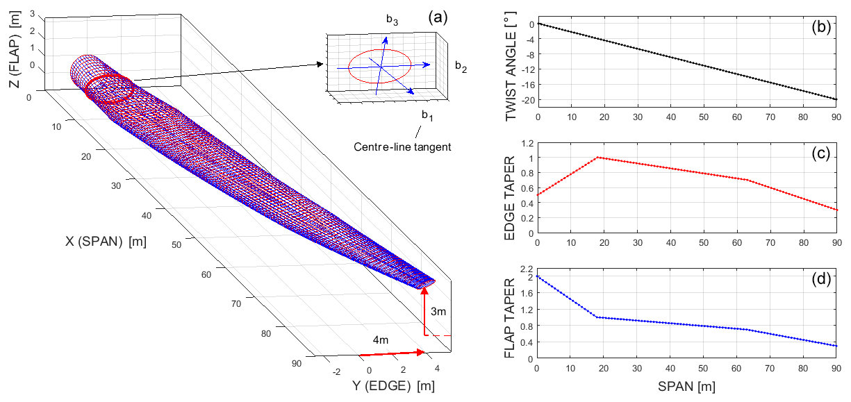
Figure 2 Example curved, twisted and tapered beamlike structure and local frame (a) and taper and twist functions (b–d).

The positions of the points in the current state are defined in a similar manner by means of the (current) mapping function:

$$\begin{array}{}\text{(12)}& R_A\left(z_i,t\right)=R_{\mathrm{0}A}\left(z_{\mathrm{1}},t\right)+x_{\mathit{\alpha }}\left(z_i\right)a_{\mathit{\alpha }}\left(z_{\mathrm{1}},t\right)+w_k\left(z_i,t\right)a_k\left(z_{\mathrm{1}},t\right),\end{array}$$

where R_0A is a function mapping the position of the centre-line points in the current state, while w_k is the components of the 3D warping displacements in local frame a_k. The main formal difference between the reference map and the current one is due to the warping, w, introduced to describe the geometry of the deformed state without a priori approximation.

By using maps (Eqs. 9 and 12), we can determine the 3D tensor, H, expressing the gradient of the current position, R_A, with respect to the reference position, R_B, as follows (see, for example, Rubin, 2000):

$$\begin{array}{}\text{(13)}& H={\displaystyle \frac{\partial R_A}{\partial R_B}}={\mathit{G}}_k\otimes {\mathit{g}}^k.\end{array}$$

In Eq. (13), G_k and g^k are covariant and contravariant base vectors, in the current state and reference states, and can be calculated by using standard mathematical methods (see, for example, Rubin, 2000). In this case they can be written in the form

$$\begin{array}{}\text{(14)}& \begin{array}{rl}& g^{\mathrm{1}}=g_{\mathrm{0}}^{-\mathrm{1}/\mathrm{2}}{b}_{\mathrm{1}},\\ & g^{\mathrm{2}}={\mathrm{\Lambda }}_{\mathrm{22}}^{-\mathrm{1}}\left(b_{\mathrm{2}}-K_{B\mathrm{2}\mathit{\alpha }}^{*}{z}_{\mathit{\alpha }}{g}_{\mathrm{0}}^{-\mathrm{1}/\mathrm{2}}{b}_{\mathrm{1}}\right),\\ & g^{\mathrm{3}}={\mathrm{\Lambda }}_{\mathrm{33}}^{-\mathrm{1}}\left(b_{\mathrm{3}}-K_{B\mathrm{3}\mathit{\alpha }}^{*}{z}_{\mathit{\alpha }}{g}_{\mathrm{0}}^{-\mathrm{1}/\mathrm{2}}{b}_{\mathrm{1}}\right),\\ & G_{\mathrm{1}}=a_{\mathrm{1}}+{\mathit{\gamma }}_i{a}_i+K_{Ai\mathit{\alpha }}^{*}{z}_{\mathit{\alpha }}{a}_i+K_{Aij}{w}_j{a}_i+w_{i,\mathrm{1}}{a}_i,\\ & G_{\mathrm{2}}={\mathrm{\Lambda }}_{\mathrm{22}}{a}_{\mathrm{2}}+w_{i,\mathrm{2}}{a}_i,\\ & G_{\mathrm{3}}={\mathrm{\Lambda }}_{\mathrm{33}}{a}_{\mathrm{3}}+w_{i,\mathrm{3}}{a}_i,\end{array}\end{array}$$

where

$$\begin{array}{}\text{(15)}& \begin{array}{rl}& g_{\mathrm{0}}^{\mathrm{1}/\mathrm{2}}=\mathrm{1}+K_{B\mathrm{1}\mathit{\alpha }}^{*}{z}_{\mathit{\alpha }},\\ & K_{\left(B\mathrm{or}A\right)i\mathit{\alpha }}^{*}={\mathrm{\Lambda }}_{i\mathit{\alpha }}^{\prime }+{\mathrm{\Lambda }}_{\mathit{\beta }\mathit{\alpha }}{K}_{\left(B\mathrm{or}A\right)i\mathit{\beta }}.\end{array}\end{array}$$

When H is known, the 3D Green–Lagrange strain tensor, E, can be calculated (see, for example, Rubin, 2000; Gurtin, 1981). Hereafter we write tensor E in a form based on simplifying assumptions applicable to the considered beamlike structure. In particular, we introduce the characteristic dimension of the cross sections, herein denoted as h, and the longitudinal dimension of the centre line, herein denoted as L, and we assume h to be much smaller than L. Moreover, we consider a thin structure and assume the curvatures of its reference centre line to be much smaller than 1∕h (see also Rubin, 2000). In addition, we assume the warping displacements, w_k, are small. More precisely, by introducing a non-dimensional parameter ε much smaller than 1, they come to be considered on the order of hε, while the order of magnitude of their derivative with respect to z₁ is εh∕L. In general, all deformation measures, i.e. the 1D strain measures γ and k and the components of the 3D strain tensor, E, are assumed to be small. In particular, their order of magnitude is at most ε. For the considered structure, in the case of small strains and small local rotations, we write the strain tensor, E, in the following form:

$$\begin{array}{}\text{(16)}& E\simeq {\displaystyle \frac{T^{T}H+H^{T}T}{\mathrm{2}}}-I.\end{array}$$

Let us now calculate the components of E by using Eq. (16) and neglecting terms smaller than ε. Algebraic manipulations, which are based on Eqs. (13)–(16), yield the following expressions for bi-tapered cross sections:

$$\begin{array}{}\text{(17)}& \begin{array}{rl}& E_{\mathrm{11}}={\mathit{\gamma }}_{\mathrm{1}}+k_{\mathrm{2}}{\mathrm{\Lambda }}_{\mathrm{33}}{z}_{\mathrm{3}}-k_{\mathrm{3}}{\mathrm{\Lambda }}_{\mathrm{22}}{z}_{\mathrm{2}},\\ & E_{\mathrm{22}}={\mathrm{\Lambda }}_{\mathrm{22}}^{-\mathrm{1}}{w}_{\mathrm{2},\mathrm{2}},\\ & E_{\mathrm{33}}={\mathrm{\Lambda }}_{\mathrm{33}}^{-\mathrm{1}}{w}_{\mathrm{3},\mathrm{3}},\\ & \mathrm{2}{E}_{\mathrm{21}}={\mathit{\gamma }}_{\mathrm{2}}+{\mathrm{\Lambda }}_{\mathrm{22}}^{-\mathrm{1}}{w}_{\mathrm{1},\mathrm{2}}-k_{\mathrm{1}}{\mathrm{\Lambda }}_{\mathrm{33}}{z}_{\mathrm{3}},\\ & \mathrm{2}{E}_{\mathrm{31}}={\mathit{\gamma }}_{\mathrm{3}}+{\mathrm{\Lambda }}_{\mathrm{33}}^{-\mathrm{1}}{w}_{\mathrm{1},\mathrm{3}}+k_{\mathrm{1}}{\mathrm{\Lambda }}_{\mathrm{22}}{z}_{\mathrm{2}},\\ & \mathrm{2}{E}_{\mathrm{23}}={\mathrm{\Lambda }}_{\mathrm{33}}^{-\mathrm{1}}{w}_{\mathrm{2},\mathrm{3}}+{\mathrm{\Lambda }}_{\mathrm{22}}^{-\mathrm{1}}{w}_{\mathrm{2},\mathrm{2}}.\end{array}\end{array}$$

In Eq. (17), Λ₂₂ and Λ₃₃ are the edgewise and flapwise taper coefficients (see, for example, Fig. 2), while the components of the strain tensor, E, are taken with respect to the reference local frame b_i; i.e.

$$\begin{array}{}\text{(18)}& E_{ij}=E\cdot b_i\otimes b_j,\end{array}$$

where “⋅” is the usual scalar (or dot) product and ⊗ is the tensor (or dyadic) product (see, for example, Rubin, 2000).

3.2 Stress fields and constitutive models

Given the strain tensor, E, the stress fields in the structure can be calculated when a constitutive model is chosen. Limiting our attention to elastic bodies, in a purely mechanical theory, in the case of small strain, we use the following linear relation between the second Piola–Kirchhoff stress tensor, S, and the Green–Lagrange strain tensor (see, for example, Gurtin, 1981):

$$\begin{array}{}\text{(19)}& S=\mathrm{2}\mathit{\mu }E+\mathit{\lambda }trEI,\end{array}$$

where μ and λ are known material parameters related to Young's modulus and Poisson's ratio. In the case of small strains and small local rotations, we also write

$$\begin{array}{}\text{(20)}& P\simeq TS,C\simeq TS{T}^T,\end{array}$$

where P is the first Piola–Kirchhoff stress tensor and C is the Cauchy stress tensor (Gurtin, 1981). It is worth noting that in the considered case the tensor field T is sufficient to determine two of the above-mentioned stress tensors (e.g. P and C) when the other one (e.g. S) is known.

We are now in a position to define the cross-sectional stress resultants, namely the force F and moment M. Using the first Piola–Kirchhoff stress tensor (Gurtin, 1981), in the case of small warpings, small strains and small local rotations, we write

$$\begin{array}{}\text{(21)}& F=T\underset{\mathrm{\Sigma }}{\int }{P}_{i\mathrm{1}}{b}_i,M=T\underset{\mathrm{\Sigma }}{\int }{x}_{\mathit{\alpha }}{P}_{i\mathrm{1}}{b}_{\mathit{\alpha }}\wedge b_i,\end{array}$$

where Σ is the domain corresponding to the cross section on which the integration is performed and

$$\begin{array}{}\text{(22)}& P_{ij}=P\cdot a_i\otimes b_j.\end{array}$$

By combining Eqs. (16)–(21), the force and moment stress resultants can be related to the geometrical parameters of the structure and the 1D strain measures (Eq. 8). However, such relations are actually known only if we know the warping fields w_k. One approach to obtaining suitable warping fields is illustrated in Sect. 3.4.

3.3 Expended power and balance equations

To complete the formulation, we conclude with considerations on the principle of expended power and the balance equations for the considered structure. For hyper-elastic bodies (Gurtin, 1981), we write the principle of expended power in the form

$$\begin{array}{}\text{(23)}& \underset{A}{\int }p\cdot v+\underset{V}{\int }b\cdot v={\displaystyle \frac{\mathrm{d}}{\mathrm{d}t}}\underset{V}{\int }\mathrm{\Phi }.\end{array}$$

In Eq. (23), p is surface loads per unit reference surface (A); b is body loads per unit reference volume (V); Φ is the 3D energy density function of the body, which is half the scalar product of the tensor fields S and E (i.e. 2$\mathrm{\Phi }=S\cdot E$); and, finally, v is the time rate of change in the current position of the body's points, which is given by

$$\begin{array}{}\text{(24)}& v=v_{\mathrm{0}}+\mathit{\omega }\wedge x_{\mathit{\alpha }}{a}_{\mathit{\alpha }}+\dot{w},\end{array}$$

where the last term in Eq. (24) is the time rate of change in the warping displacement.

For small warpings, small strains and small local rotations, if the power expended by surface and body loads on the warping velocities is neglected, the external power, Π_e, reduces to the following form:

$$\begin{array}{}\text{(25)}& {\mathrm{\Pi }}_{\mathrm{e}}=\mathrm{\Delta }\left(F\cdot {\mathit{v}}_{\mathrm{0}}+M\cdot \mathit{\omega }\right)+\underset{s}{\int }{F}_{\mathrm{s}}\cdot {\mathit{v}}_{\mathrm{0}}+M_{\mathrm{s}}\cdot \mathit{\omega },\end{array}$$

where the vector field v₀ is the time rate of change in the position of the current centre-line points, the vector field ω is the time rate of change in the orientation of vectors a_i, and the terms F_s and M_s are suitable resultants of inertial actions and prescribed loads per unit length in the reference state, while the symbol Δ simply indicates that the function between brackets is evaluated at both the ends of the beam and the difference between those values is taken.

The cross-sectional warpings may be important in calculating the 3D energy function and cannot be neglected in the internal power, Π_i. However, the internal power may be reduced to a useful form for beamlike structures by introducing a suitable 1D strain energy function, U. For example, if U can be expressed in terms of the strain measures, γ and k, we can write

$$\begin{array}{}\text{(26)}& {\mathrm{\Pi }}_i={\displaystyle \frac{\mathrm{d}}{\mathrm{d}t}}\underset{s}{\int }U(\mathit{\gamma },k,s)=\underset{s}{\int }f\cdot \dot{\mathit{\gamma }}+m\cdot \dot{k},\end{array}$$

where the vector fields f and m are defined in terms of the force and moment stress resultants, F and M, as follows:

$$\begin{array}{}\text{(27)}& f=T^{T}F,m=T^{T}M.\end{array}$$

By using the principle of expended power, we also obtain balance equations for the vector fields F and M in the form

$$\begin{array}{}\text{(28)}& \begin{array}{rl}& F^{\prime }+F_{\mathrm{s}}=\mathrm{0},\\ & M^{\prime }+R_{\mathrm{0}A}^{\prime }\wedge F+M_{\mathrm{s}}=\mathrm{0}.\end{array}\end{array}$$

At this point, we have kinematic equations, Eqs. (6) and (7); strain measures, Eqs. (8) and (16); force and moment balance equations, Eq. (28); and the principle of expended power, Π_e=Π_i, in a suitable form for beamlike structures, Eqs. (25) and (26). To complete the formulation of the model we need relations providing the 1D stress resultants in terms of the 1D strain measures. To this end, we need to know the warping fields. An approach to obtaining suitable warping functions is discussed in the next section.

3.4 Warping displacements

In general, a 3D non-linear elasticity problem can be formulated as a variational problem. However, if we try to solve the variational problem directly, the difficulties encountered in solving the elasticity problem remain. For beamlike structures whose transversal dimensions are much smaller than the longitudinal one, assumptions based on the shape of the structure and the smallness of the warping and strain fields can lead to useful simplifications. In particular, solving the 3D non-linear elasticity problem can be reduced to solutions of two main problems. See, for example, Berdichevsky (1981), who seems to be the first in the literature to plainly state this for elastic rods. One of the two problems governs the local distortion of the cross sections and is referred to here as the cross-section problem. The other governs the global deformation of the centre line and is referred to here as the centre-line problem. Hereafter, we consider the following variational statement to determine the warping fields which are responsible for deformation of the cross sections:

$$\begin{array}{}\text{(29)}& \mathit{\delta }\underset{V}{\int }\mathrm{\Phi }=\mathrm{0}.\end{array}$$

In Eq. (29) the symbol δ stands for the variation operator and the density function Φ depends on the warping displacements. The warping fields satisfying Eq. (29) can be obtained by the corresponding Euler–Lagrange equations (see, for example, Courant and Hilbert, 1953), by using numerical methods, in general, or analytical approaches providing closed-form expressions, in some particular cases. Once such a problem is solved, the components of the stress resultants (Eq. 21) can be linearly related to the components of the 1D strain measures by using Eqs. (16)–(21). Then, if it is preferred or deemed useful, the resulting relations can also be arranged in a standard matrix form.

Note that to determine the current state of the structure, we also need the displacements of its centre-line points. They can be determined by solving the centre-line problem, which is a non-linear problem governed by the set of kinematic, constitutive and balance equations introduced in Sect. 3 (in particular, we are referring to the constitutive model in Sect. 3.2, which relates stress resultants and strain measures, and the balance equations for the stress resultants in Sect. 3.3).

In the next sections we show some analytical solutions (Sect. 4) and numerical results (Sect. 5) that can be obtained by applying the proposed modelling approach to some reference beamlike structures.

4 First analytical results for bi-tapered cross sections

In this section we consider the case of a beamlike structure with bi-tapered elliptical cross sections. For this case we can obtain analytical solutions in terms of warping fields, while for generic shapes (e.g. the aerodynamic profiles used in wind and steam turbine blades as well as helicopter rotor blades) the problem corresponding to Eq. (29) can be solved using numerical methods. However, this is not surprising, since analytical solutions are available only for a limited number of cases even in the classical linear theory of prismatic beams (see, for example, Love, 1944).

As discussed in Sect. 3, we are assuming that the warpings, strains and local rotations are small. Moreover, hereafter we choose that the current local frames be tangent to the current centre line and include possible shear deformations within the warping fields. In addition, with the aim of showing a first analytical solution for bi-tapered cross sections, here we neglect the effects of the initial cross-sectional twist. Then, we write the Euler–Lagrange equations corresponding to Eq. (29), whose unknown functions are the warping fields, w_k (this can be done using standard mathematical techniques; see, for example, Courant and Hilbert, 1953). Finally, we proceed to find a solution to the resulting (partial differential equations) problem. In particular, if we neglect the terms smaller than ε and maintain those related to extension, γ₁, and changes in curvature, k_i, the aforementioned Euler–Lagrange equations are satisfied by the following warping fields:

$$\begin{array}{}\text{(30)}& \begin{array}{rl}& w_{\mathrm{1}}=k_{\mathrm{1}}{\displaystyle \frac{{\mathit{\rho }}^{\mathrm{2}}{d}_{\mathrm{3}}^{\mathrm{2}}-d_{\mathrm{2}}^{\mathrm{2}}}{{\mathit{\rho }}^{\mathrm{2}}{d}_{\mathrm{3}}^{\mathrm{2}}+d_{\mathrm{2}}^{\mathrm{2}}}}\mathit{\rho }{\mathrm{\Lambda }}^{\mathrm{2}}{z}_{\mathrm{2}}{z}_{\mathrm{3}},\\ & w_{\mathrm{2}}=-\mathit{\nu }{\mathit{\gamma }}_{\mathrm{1}}\mathrm{\Lambda }{z}_{\mathrm{2}}-\mathit{\nu }{k}_{\mathrm{2}}\mathit{\rho }{\mathrm{\Lambda }}^{\mathrm{2}}{z}_{\mathrm{2}}{z}_{\mathrm{3}}+\mathit{\nu }{k}_{\mathrm{3}}{\mathrm{\Lambda }}^{\mathrm{2}}\left({\mathit{\rho }}^{\mathrm{2}}{z}_{\mathrm{3}}^{\mathrm{2}}-z_{\mathrm{2}}^{\mathrm{2}}\right)/\mathrm{2},\\ & w_{\mathrm{3}}=-\mathit{\nu }{\mathit{\gamma }}_{\mathrm{1}}\mathit{\rho }\mathrm{\Lambda }{z}_{\mathrm{3}}+\mathit{\nu }{k}_{\mathrm{3}}\mathit{\rho }{\mathrm{\Lambda }}^{\mathrm{2}}{z}_{\mathrm{2}}{z}_{\mathrm{3}}-\mathit{\nu }{k}_{\mathrm{2}}{\mathrm{\Lambda }}^{\mathrm{2}}\left({\mathit{\rho }}^{\mathrm{2}}{z}_{\mathrm{3}}^{\mathrm{2}}-z_{\mathrm{2}}^{\mathrm{2}}\right)/\mathrm{2},\end{array}\end{array}$$

where d₂ and d₃ are the major semi-axes of a reference elliptical cross section (e.g. the one at 18m from the root section in Fig. 2), while Λ=Λ₂₂ and $\mathit{\rho }={\mathrm{\Lambda }}_{\mathrm{33}}/{\mathrm{\Lambda }}_{\mathrm{22}}$ are known functions of z₁. Using this result, we can calculate the corresponding strain and stress fields, Eqs. (16)–(20), stress resultants, Eq. (21), and strain energy function U. For example, if we consider a local frame in the reference cross section with its origin at the cross section's centre of mass and its axes aligned with the cross section's principal axes of inertia (as in Fig. 2), we can write the 1D strain energy function, U, in the form

$$\begin{array}{}\text{(31)}& \begin{array}{rl}U& ={\displaystyle \frac{\mathrm{1}}{\mathrm{2}}}EA\mathit{\rho }{\mathrm{\Lambda }}^{\mathrm{2}}{\mathit{\gamma }}_{\mathrm{1}}^{\mathrm{2}}+{\displaystyle \frac{\mathrm{1}}{\mathrm{2}}}G{J}_{\mathrm{1}}{\mathit{\rho }}^{\mathrm{2}}{\mathrm{\Lambda }}^{\mathrm{4}}{k}_{\mathrm{1}}^{\mathrm{2}}+{\displaystyle \frac{\mathrm{1}}{\mathrm{2}}}E{J}_{\mathrm{2}}{\mathit{\rho }}^{\mathrm{3}}{\mathrm{\Lambda }}^{\mathrm{4}}{k}_{\mathrm{2}}^{\mathrm{2}}\\ & +{\displaystyle \frac{\mathrm{1}}{\mathrm{2}}}E{J}_{\mathrm{3}}\mathit{\rho }{\mathrm{\Lambda }}^{\mathrm{4}}{k}_{\mathrm{3}}^{\mathrm{2}}.\end{array}\end{array}$$

In Eq. (31), E is the Young modulus and G is the shear modulus, while A, J₁, J₂ and J₃ are the following geometrical parameters:

$$\begin{array}{}\text{(32)}& \begin{array}{rl}& A=\mathit{\pi }{d}_{\mathrm{2}}{d}_{\mathrm{3}},J_{\mathrm{1}}=A{d}_{\mathrm{2}}^{\mathrm{2}}{d}_{\mathrm{3}}^{\mathrm{2}}/\left(\mathit{\rho }{d}_{\mathrm{3}}^{\mathrm{2}}+{\mathit{\rho }}^{-\mathrm{1}}{d}_{\mathrm{2}}^{\mathrm{2}}\right),\\ & J_{\mathrm{2}}=A{d}_{\mathrm{3}}^{\mathrm{2}}/\mathrm{4},J_{\mathrm{3}}=A{d}_{\mathrm{2}}^{\mathrm{2}}/\mathrm{4}.\end{array}\end{array}$$

An interesting result is that the initial taper appears explicitly in all the previous relations (in terms of ρ and Λ). This, in turn, allows analytical evaluation of its effects on the 3D strain fields, which can be calculated by using Eqs. (17) and (30) and are, in any case, required to determine the 3D stress fields (Eq. 19).

5 Numerical simulations

In this section we present the results of simulations conducted using the modelling approach discussed in Sect. 3, which we have implemented into a numerical code in MATLAB language. The results are also compared with those obtainable via 3D FEM simulations with the commercial software ANSYS.

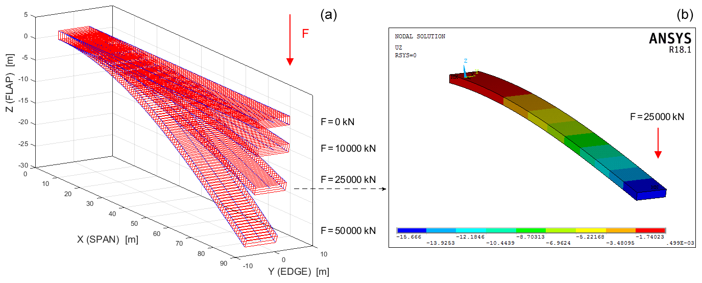
Figure 3 Global deformation with 3D BLM for increasing F (a) and with 3D FEM for F=25 000 kN (b).

In particular, we show a first set of test cases in which a beamlike structure with rectangular cross sections undergoes large displacements while fixed at one end and loaded at the other by a force of progressively increasing magnitude. The second set of test cases addresses a more complex geometry, that is, a beamlike structure with elliptical cross sections, which is curved, twisted and tapered in its reference configuration and under the same loading condition as in the first set of test cases. Finally, the third set of test cases regards four different beamlike structures under the same loading conditions. In particular, we consider a first prismatic structure with elliptical cross sections. The second structure is a modification of the first, on which the same cross section is maintained at 18 m from the root, while taper is added according to the taper coefficients in Fig. 2. Starting with this latter structure, we then consider a third structure which includes twisting of the cross sections, assuming the twist law in Fig. 2. The fourth and final case is a curved, twisted and tapered structure obtained from the third (tapered and twisted) by adding a centre-line curvature. Once the simulations have been completed, we compare the results obtained to highlight the effects of their different geometries on their mechanical behaviour.

In all cases, the displacements of the reference centre-line points are calculated by solving the centre-line non-linear problem through the previously mentioned numerical procedure we have implemented in MATLAB, which is based on the kinematic, constitutive and balance equations introduced in Sect. 3. In particular, the constitutive model introduced in Sect. 3.2 is used to relate stress resultants and strain measures. We define the local frames orientation using Euler angles and simulate orientation changes in terms of the derivatives of those angles over the arch length, s (see, for example, Pai, 2014). We use the balance equations for the stress resultants introduced in Sect. 3.3. Finally, the resulting set of ordinary differential equations is (numerically) integrated with respect to the reference arch length, s. The results of this procedure are illustrated in the following sections.

5.1 First set of test cases

In this set of test cases we consider a rectangular cross-sectioned beamlike structure which undergoes large displacements while clamped at one end (i.e. the root) and loaded at the other (i.e. the tip) by a force, F, whose magnitude is progressively increased (see Fig. 3). The centre-line length is d₁=90 m, while the cross-section dimensions are d₂=8 m (edgewise) and d₃=2 m (flapwise). The material properties are summarized by reference values of Young's modulus, 70 GPa, and Poisson's ratio, 0.25. Finally, the flapwise tip force, F, varies from 100 to 75 000 kN.

The simulations are run for different values of the tip force. The model we have implemented in MATLAB for solving the non-linear problem renders results on the structure's deformed configuration (e.g. Fig. 3a) within a few seconds. In all cases, the simulation time is less than 2.4 s, which is significantly less than that required for the corresponding non-linear 3D FEM simulations carried out on the same computer, while the accuracy of the results is almost the same. A summary of the results obtained, in terms of global displacements and simulation times, is shown in Figs. 3 and 4.

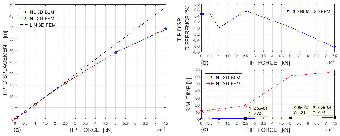
Figure 4 Comparison of tip displacements (a), tip displacement differences (b) and simulation times (c).

In particular, Fig. 3b shows the undeformed shape (for F=0), as well as the deformed shapes for F equal to 10 000, 25 000 and 50 000 kN. Figure 3b shows the 3D FEM deformed shape for F=25 000 kN (the coloured scale is for the flapwise displacements). Figure 4a provides a comparison between the tip displacements obtained with the linear 3D FEM, the non-linear 3D FEM and our model (indicated as 3D BLM). It also shows the differences (between the non-linear 3D FEM and the 3D BLM) in terms of tip displacements and simulation times for the considered cases.

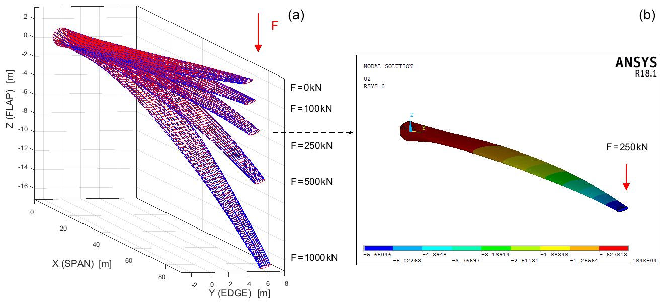
Figure 5 Global deformation with 3D BLM for increasing F (a) and with 3D FEM for F=250 kN (b).

5.2 Second set of test cases

Let us now consider a more complex beamlike structure, specifically, one with a 90 m curved centre line with constant curvatures, which schematizes a pre-bent and swept beam whose tip is moved 4 m edgewise and 3 m flapwise, as in Fig. 2. The local frames in the reference state are characterized by a pre-twist of 20^∘ m⁻¹. The reference cross section at 18 m from the root is an ellipse whose major semi-axes are d₂=2 m (edgewise) and d₃=0.5 m (flapwise). The sizes of the other cross sections change according to the taper coefficients in Fig. 2. The material properties are represented by reference values of Young's modulus, 70 GPa, and Poisson's ratio, 0.25. Finally, the structure is clamped at its root and loaded by a flapwise tip force, F, which varies from 100 to 1000 kN.

The simulations are run for different values of tip force, F. The model we have implemented in MATLAB for solving the non-linear problem yields results regarding the structure's deformed configurations, such as those in Fig. 5, which confirm the computational efficiency and accuracy observed in the previous tests. In particular, simulation times are significantly shorter than those required by corresponding non-linear 3D FEM simulations (see, for example, the simulation times ratio in Fig. 6c), while the accuracy of the results is again nearly the same (Fig. 6).

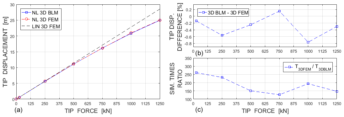
Figure 6 Comparison of tip displacements (a), tip displacement differences (b) and simulation times ratio (c).

Figure 7 Displacement of the reference centre-line points with 3D BLM for increasing F.

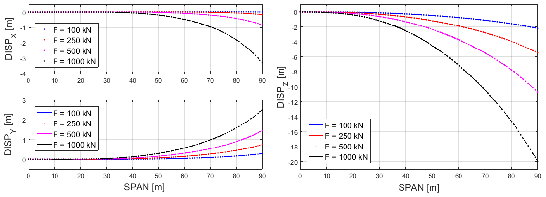
Apart from the foregoing results, the model is also able to provide other meaningful information. In particular, we can obtain the displacement fields of the reference centre-line points (Fig. 7), as well as the change in curvature of the beamlike structure (Fig. 8a–c) and the corresponding moment stress resultant (Fig. 8d–f). The moment components are in the current local frame, a_i, whose orientation has been determined as part of the solution to the non-linear problem. For example, the orientation of the current local frame, a_i, can be expressed in terms of a set of Euler angles, as in Fig. 9. In this case we have considered the set of Euler angles corresponding to a first rotation, θ, about the initial z axis; a second rotation, γ, about the intermediate y axis; and a third rotation, ψ, about the final x axis.

Figure 8 Changes in curvature (a–c) and moment stress resultants (d–f) with 3D BLM for increasing F.

Figure 9 Local frame orientations in terms of Euler angles before (green lines) and after deformation.

5.3 Third set of test cases

The last test cases regard four different beamlike structures, starting with a prismatic elliptical one, to which there is the step-by-step addition of the taper; the twist of the cross sections; and, finally, the curvature of the centre line, as discussed in Sect. 5. Note that the curved–twisted–tapered case considered here coincides with that discussed in more detail in Sect. 5.2 (see Figs. 5–9, F=250 kN). We begin by simulating the behaviour of these four structures under a flapwise tip force of 250 kN. Then, we analyse the results obtained to show the effect of the geometrical differences on their mechanical behaviour. The results obtained are summarized in the following. In particular, Fig. 10 shows the reference and deformed states of the prismatic structure (Fig. 10a) and the deformed states of the non-prismatic ones (Fig. 10b), while Fig. 11 shows the displacements of their centre-line points. The main effect of the considered tip force is a displacement in the z direction in all cases, with a displacement in the y direction for the tapered–twisted and tapered–twisted–curved cases only, as would be expected.

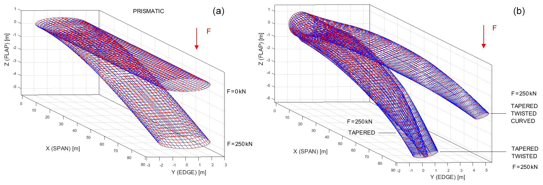
Figure 10 Prismatic case before and after deformation (a) and non-prismatic cases after deformation (b).

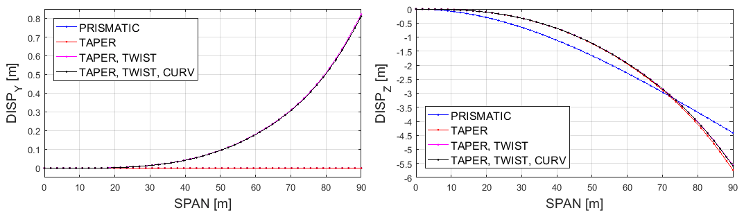
Figure 11 Centre-line points displacement of prismatic case (blue) and non-prismatic cases (other colours) for F=250 kN.

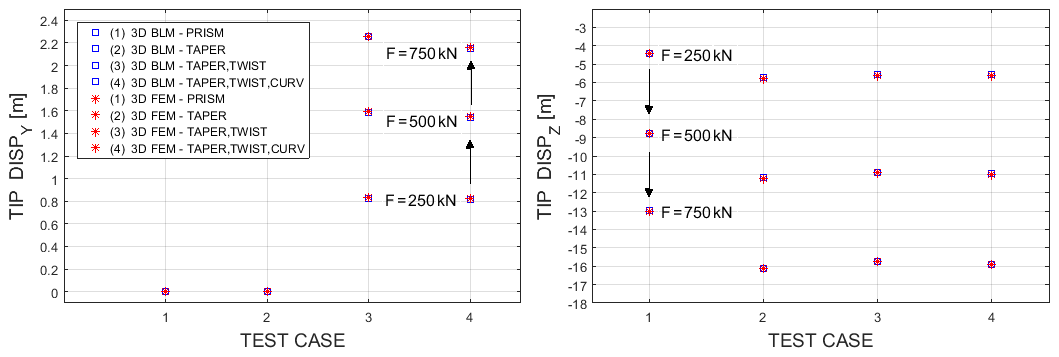
Figure 12 Tip displacements with 3D BLM (blue) and 3D FEM (red) for different geometries and increasing F (see arrows).

Similar results have also been obtained for larger values of tip force, F, which lead to larger tip displacements. In particular, hereafter we show the results for F varying from 250 to 750 kN. As for the previous test cases, the results obtained have been compared with those from 3D FEM simulations, confirming the computational efficiency and accuracy revealed in the previous sections. A summary is shown in Fig. 12, which provides a comparison in terms of tip displacements, for the four geometries considered here for F=250, F=500 and F=750 kN. Such loads correspond, respectively, to tip displacements of about 6.4 %, 12.5 % and 18.1 % of the spanwise reference length. The difference between the 3D BLM and the non-linear 3D FEM in terms of tip displacements is below 0.9 % in all the considered cases (Fig. 12).

We conclude now by examining the results for the 3D strain measure E₁₁, also referred to as longitudinal strain, which is another important parameter for the analysis and design of rotor blades (see, for example, Griffith and Ashwill, 2011). In particular, we focus on the effects of taper by considering a beamlike structure with bi-tapered cross sections (test case 2 in Fig. 12). Then, we compare the outcomes of the 3D BLM with those of linear and non-linear 3D FEM simulations. A summary of the results is reported in Fig. 13, which shows the maximum longitudinal strain at different reference cross sections (at 30 %, 50 % and 70 % of the spanwise reference length) and for three different tip forces (F=250, F=500 and F=750 kN).

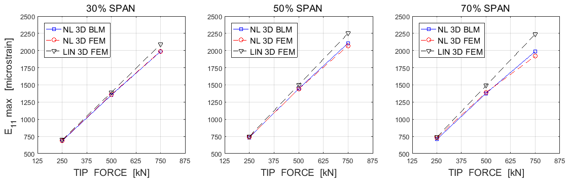
Figure 13 Max longitudinal strain E₁₁ in cross sections at 30 %, 50 % and 70 % span for increasing F (bi-tapered case).

As verified by many simulations and shown in the examples, the proposed approach performs well in terms of computational efficiency and accuracy. It can be used to study the mechanical behaviour of beamlike structures, which are curved, twisted and tapered in their unstressed reference state and undergo large global displacements. It can moreover provide information on the deformed configurations of the structures, such as their displacement fields, as well as the corresponding strain and stress measures. It is worth noting that it is suitable for beamlike structures with generic reference cross-sections shapes. However, as already pointed out, for bi-tapered elliptical cross sections, analytical solutions can be obtained in terms of warping fields, while for generic reference cross-section shapes problem, Eq. (29) has to be solved using numerical methods.

6 Conclusions

Many complex engineering structures, such as the rotor blades of wind turbines and helicopters, are non-prismatic beamlike structures, with one dimension much larger than the other two and a shape that is curved, twisted and also tapered in the unstressed reference state. The increasing size and flexibility of such structures make the prediction of their aeroelastic behaviour ever more challenging. This paper addressed the structural part of this modelling and proposed a modelling approach, referred to as 3D BLM, which is computationally efficient, accurate and explicitly considers the main geometrical characteristics of the mentioned structures, the large deflections of their reference centre line, and the in- and out-of-plane warping of their transversal cross sections. In the mentioned approach, the warping displacements have been thought of as an additional small motion superimposed on the global motion of the local frames. The strain tensor has been calculated analytically in terms of geometrical parameters of the structure, 1D strain measures and 3D warping fields. A method based on a variational statement has been used to obtain suitable warping fields. The proposed approach enables one to obtain analytical results in particular cases and can be implemented into an efficient numerical code in the general case. The analytical results obtained, along with numerical examples (obtained by implementing 3D BLM into a computer code) and comparisons with corresponding results from 3D FEM simulations, have been presented to show the effectiveness of the modelling approach and the information it can provide. In all cases, the simulation times with 3D BLM have been significantly shorter than those required by 3D FEM simulations, while the accuracy of the results has been always almost the same. In this paper the analyses have been limited to the terms of order ε, as discussed when introducing the strain measures of the model. This turned out to be sufficient to accurately predict the global deflection of the considered structures even when the displacements of the centre-line points are large and non-linear with respect to the applied loads. The inclusion of higher-order terms in the model may provide better results, especially in terms of stress and strain field predictions, while not practically affecting the computational performance of the implemented model. This is an important point to be further investigated and will be the objective of a successive work. An interesting future activity would also be to performing comparison analyses with other structural modelling methods (not only 3D FEM), with the aim of assessing the performance of different structural models for non-prismatic beamlike structures in terms of the information each approach can provide (e.g. centre-line displacements, 1D strain measures, 3D strain fields), computational efficiency and results accuracy.