the Creative Commons Attribution 4.0 License.
the Creative Commons Attribution 4.0 License.
 | 23 Jun 2020
Two-dimensional numerical simulations of vortex-induced vibrations for a cylinder in conditions representative of wind turbine towers
Adriaan Derksen
Mikko Folkersma
Kumayl Sarwar
Vortex-induced vibrations (VIVs) of wind turbine towers can be critical during the installation phase, when the rotor–nacelle assembly is not yet mounted on the tower. The present work uses numerical simulations to study VIVs of a two-dimensional cylinder in the transverse direction under flow conditions that are representative of wind turbine towers both from a fluid dynamics and structural dynamics perspective. First, the numerical tools and fluid–structure interaction algorithm are validated by considering a cylinder vibrating freely in a laminar flow. In that case, both the motion amplitude and frequency are shown to agree well with previous results from the literature. Second, VIVs are modelled in the turbulent supercritical regime using unsteady Reynolds-averaged Navier–Stokes equations. In this context, the turbulence model is first validated against flow past a stationary cylinder with a high Reynolds number. Then, the results from forced vibrations are validated against experimental results for a range of reduced frequencies and velocities. It is shown that the behaviour of the aerodynamic damping changes with the frequency ratio and can therefore lead to either self-limiting or self-exciting VIVs when the cylinder is left to freely vibrate. Finally, results are shown for a freely vibrating cylinder under realistic flow and structural conditions. While a clear lock-in map is identified and shows good agreement with published numerical and experimental data, the work also highlights the unsteady nature of the aerodynamic forces and motion under certain operating conditions.
- Article
(3868 KB) - Full-text XML
- BibTeX
- EndNote


Vortex-induced vibrations (VIVs) are structural vibrations that can occur due to the shedding of flow vortices when a fluid flow passes around a structure. Due to this fluid–structure interaction (FSI) phenomenon, a synchronization (also called lock-in) of the vortex shedding and the structural motion can occur for certain flow conditions and/or structural properties, leading to premature fatigue failures. Vortex-induced vibrations occur in many engineering applications, such as suspension bridges, marine risers, and industrial chimneys. In the context of wind energy, such vibrations have been observed numerically both in the tower (Livanos, 2018; Derksen, 2019) and the wind turbine rotor (Heinz et al., 2016; Horcas et al., 2019). The increase in rotor height and diameter makes VIVs an increasingly problematic issue when designing the new generation of wind turbines. This work is motivated by the specific problem of VIVs of wind turbine towers during their installation. In that phase, when the tower does not yet support the rotor–nacelle assembly, it acts as a beam clamped at one of its ends and is subjected to wind flow. Because of the vortex shedding developing in the tower wake, the tower may start to oscillate. This is particularly critical at three different stages of the installation process, namely when the tower (i) stands on the quayside, (ii) is transported on a vessel offshore, and (iii) is installed on the offshore foundation in the absence of the rotor–nacelle assembly.
The design of wind turbine towers depends on a number of parameters (Dykes et al., 2018). The tower's natural frequency, which is important for the dynamic response of the structure to vortex-induced excitations, depends on the tower diameter, thickness, material, and geometry (tapered). Various combinations of these parameters are therefore critical for the occurrence of VIVs. For the current towers used by Siemens Gamesa Renewable Energy, it is observed that tower diameters in the range of and with a first bending frequency of are most critical for the occurrence of VIVs. However, as mentioned above, this is thickness-, material-, and shape-dependent. Furthermore, the trend over the years has been to reduce the tower-clamped first-mode frequency. This brings challenges as the critical resonance velocities are at a lower wind speed, which results in higher VIV incidences.
In practice, wind turbine towers are usually tapered cylinders with sections of discrete diameters. This shape, together with wind shear, might influence the VIV behaviour of the structure compared to that of circular cylinders. This has already been investigated to some extent in the literature (Balasubramanian et al., 2001; Hover et al., 1998; Bourguet et al., 2013; Bourguet and Triantafyllou, 2016). In this paper, however, this effect is neglected, and circular cylinders are considered instead, with a focus on large Reynolds numbers. Despite this limitation, the present study is relevant for the wind energy industry because of the interest of wind turbine developers in reducing the tapering at the top sections. The phenomenological aspects of VIVs for circular cylinders have been extensively analysed in the literature for several decades. However, studies involving large Reynolds numbers and large mass ratios (defined as the ratio between the structure mass and the mass of the displaced fluid) are still quite rare. Experiments in both air (Feng, 1968; Brika and Laneville, 1993) and water (Govardghan and Williamson, 2000) have shown that cylinders with large mass ratios exhibit much smaller amplitudes of vibrations than those with low mass ratios. Belloli et al. (2012), however, showed that this is not necessarily true in the presence of large Reynolds numbers of the order of Re=50 000. In this context, the maximum non-dimensional oscillation amplitude can become larger than the cylinder diameter. This was also described in other studies with low mass ratios (Govardghan and Williamson, 2006). For this reason, the original Griffin plot (Griffin, 1980), which describes the maximum oscillation amplitude as a function of the mass damping parameter, needs to be modified for large Reynolds numbers.
It is worth noting that all these VIV studies were limited to the subcritical regime, in which the boundary layer remains fully laminar, and the drag coefficient is nearly constant with the Reynolds number. By contrast, wind turbine towers experience flows both in the transitional regime (), where laminar separation bubbles can exist and reduce the drag coefficient, and in the supercritical regime (), in which the boundary layer is fully turbulent. Experiments in these regimes can be challenging due to the need for large wind tunnels and wind speeds. In the context of stationary cylinders, a series of experiments have been performed with these very large Reynolds numbers (Roshko, 1961; Achenbach, 1968; Jones et al., 1969; van Nunen, 1974; Schewe, 1983). These studies generally agree well with the value of the separation angle and the location of the minimum pressure coefficient. However, large discrepancies are found between the various experimental data for the values of the aerodynamic quantities, such as pressure coefficient, lift and drag coefficients, and Strouhal number. Jones et al. (1969) also looked at a circular cylinder under forced vibration. Their study showed that a lift amplification exists and is due to the cylinder motion, which is in agreement with other works. Numerical studies have also been performed for flow past 2D and 3D stationary cylinders. These include unsteady Reynolds-averaged Navier–Stokes (URANS) models (Travin et al., 2000; Catalano et al., 2003; Ong et al., 2009; Rosetti et al., 2012), large-eddy simulations (LESs; Breuer, 2000; Catalano et al., 2003; Singh and Mittal, 2005), and detached-eddy simulations (DESs; Travin et al., 2000; Squires et al., 2008). Scatter has been observed between the various URANS simulations and was attributed to either different wall function implementations or the fact that some simulations were done in 2D instead of 3D. In most cases, the numerical results also deviate from the experiments, especially with URANS simulations. The latter methodology indeed presents shortcomings, such as an isotropic eddy viscosity, homogeneous Reynolds stresses, and the modelling of the full range of turbulent eddies (Rosetti et al., 2012). Yet, it was found that URANS simulations can still lead to satisfactory engineering results in the supercritical flow regime (Ong et al., 2009). The present study will go a step further by presenting URANS results of a freely vibrating cylinder in the supercritical regime (). To the best of the authors' knowledge, this is the first numerical work to do so.
The paper is organized as follows. Section 2 presents the fluid dynamics and structural dynamics models used in this study. It also explains the algorithm used to couple these models and perform two-way coupled fluid–structure interaction (FSI) simulations of a freely vibrating cylinder. Section 3 shows the results for two different regimes. First, laminar flow is considered in order to validate both the models and the FSI algorithm. The results of a freely vibrating cylinder are presented and compared to the literature. Second, the turbulent supercritical regime is considered for three cases: stationary cylinder, cylinder undergoing forced vibrations, and cylinder undergoing free vibrations. Finally, conclusions are drawn in Sect. 4.
2.1 Fluid dynamics model
The computational fluid dynamics (CFD) model used in this study is the open-source code Open-FOAM-v1812. The model uses a finite-volume discretization of the incompressible Navier–Stokes equations for a Newtonian fluid. In the laminar regime, these equations are solved directly, without using a turbulence model, through direct numerical simulation (DNS). In the turbulent regime, the unsteady Reynolds-averaged Navier–Stokes (URANS) equations are solved using a k–ω shear stress transport (SST) turbulence model (Menter, 1994), namely
where the fluid velocity is decomposed into an averaged and a fluctuating part, i.e. with . Furthermore, p is the pressure field, ρ is the fluid density, and ν is the fluid kinematic viscosity. Additionally, the turbulence model assumes that
with δij denoting the Kronecker symbol, νt the eddy viscosity, Sij the strain rate tensor defined as
and k the turbulent kinetic energy defined as
The specific implementation of the model is that presented by Menter et al. (2003), with a revised turbulence-specific dissipation rate production term from Menter and Esch (2001). The turbulent-specific dissipation rate ω is computed by solving the following equation:
where the blending function F1 is given by
and
The transport equation for the turbulent kinetic energy k is given by
where the limited production term is given by
and
Furthermore, the values of the turbulence coefficients are given in Table 1.

If needed, the constants are blended (typically close to the boundary layer) by the following interpolation:
where ϕ represents any of the coefficients in Table 1. Once the two turbulence transport equations are solved, the eddy viscosity field is obtained as
in which Ω is the magnitude of the strain rate tensor, a1 is a coefficient defined in Table 1, and F2 is the following blending function:
The equations are discretized using second-order methods in both space and time. Only the equations for k and ω are solved using a first-order upwind scheme. The PISO-SIMPLE (PIMPLE) algorithm is used for the pressure–velocity coupling, where PISO is the pressure-implicit splitting of operators, and SIMPLE is the semi-implicit method for pressure-linked equations. This model represents the state of the art in URANS modelling. However, it does have the limitation that the model is two-dimensional and therefore cannot take vertical wind shear into account. Furthermore, it has some limitations for the boundary layer transition regime.
2.2 Structural dynamics model
The two-dimensional cylinder is modelled as a rigid body of mass m attached to a linear spring with spring constant ks and a viscous damper with damping coefficient c. The motion of the rigid body is constrained so that it cannot rotate and can only translate in the y direction, transverse to the inflow. The response of the body is therefore governed by the equations of motion of a single degree of freedom oscillator, i.e.
where , , and y are the y components of the linear acceleration, velocity, and displacement, respectively, of the centre of gravity of the structure, and Fy is the resultant traction force exerted on the structure by the fluid. Equation (15) can be written as
where is the natural frequency of the structure, and ζ is the damping coefficient defined as the ratio between the actual damping and the critical value, i.e.
For a three-dimensional tower, the values for mass, stiffness, and damping vary along the tower. Here, a modal analysis was performed to lump these values into a single value representing the two-dimensional property of the cylinder. To do so, the three-dimensional tower is divided into 40 segments with 6 degrees of freedom at each node, leading to stiffness and mass matrices of dimensions 246×246. The natural frequency of the first mode is obtained by solving Eq. (15) in the frequency domain. The modal mass and stiffness are then obtained by premultiplying and postmultiplying the mass and stiffness matrices by the eigenvector of the first bending mode. Equation (16) is further non-dimensionalized as
denoting (D being the cylinder diameter), , and . Additionally, stands for the aerodynamic coefficient expressed in terms of y*, , and the reduced velocity is .
2.3 Fluid–structure interaction coupling algorithm
In this work, fluid–structure interactions are modelled using a partitioned approach, whereby the fluid and structural dynamics are solved alternatively at every time step. Here, both weakly and strongly coupled schemes are considered. This is illustrated by Fig. 1. At the start of a new time step, Eq. (15) is solved for the structural dynamics. Once the structure displacement is known, the geometry is moved accordingly, and the mesh is diffused using a spherical linear interpolation scheme (SLERP) algorithm. With this approach, it is possible to specify a mesh region where the cells preserve their shape during motion. In this work, for the freely vibrating cases, the mesh at a distance of up to 25D around the cylinder is kept rigid throughout the simulations in order to keep its initial high-quality characteristics in the O-grid block. By contrast, the mesh deformation is applied to all cells located farther away from the cylinder. Once the mesh has moved, the fluid dynamics solver solves the Navier–Stokes equations, accounting for the mesh motion using an arbitrary Lagrangian–Eulerian approach. In the weakly coupled algorithm, the fluid dynamics equations are solved iteratively without solving again for the structural dynamics. The structural and mesh motion are then only solved once per time step. By contrast, in the strongly coupled approach, the structural dynamics equations are solved for each sub-iteration of the fluid solver. Thus, the structural dynamics and mesh movement are solved multiple times per time step.
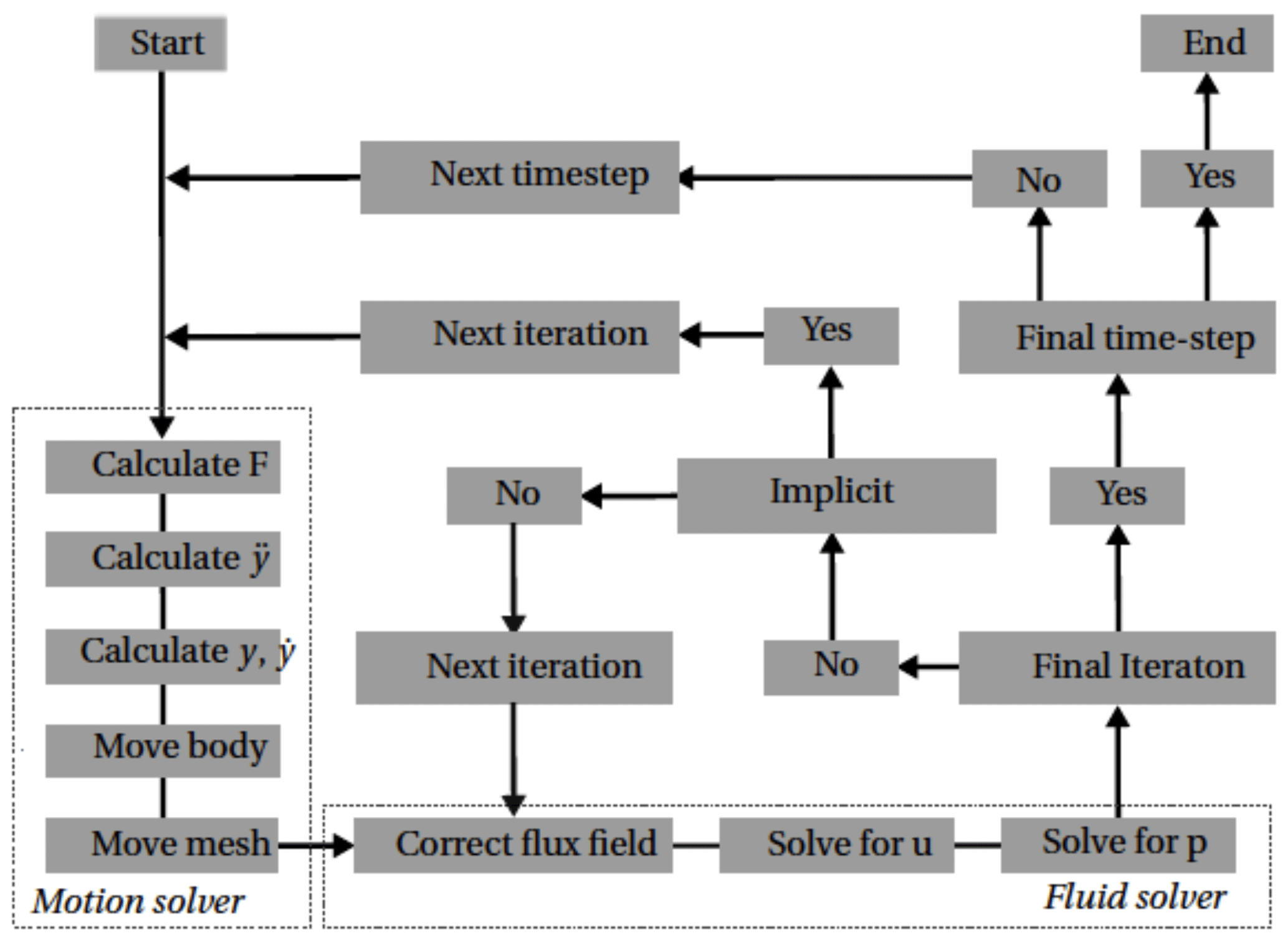
In this work, a weakly coupled algorithm was found to give accurate results for modelling VIVs in the laminar regime. In that case, the structural dynamics equations were also solved using an explicit solver, the so-called symplectic integrator (Dullweber et al., 1997), which is based on the leapfrog method. The explicit character of this solver leads to a constant structural displacement for each iteration within a time step, while the acceleration and velocity may change at each iteration. The structural displacement of the current time step is only dependent on the acceleration computed in the previous time step. In the turbulent regime, a strongly coupled FSI scheme was adopted, and three to four sub-iterations were necessary between fluid and structural solvers to achieve accurate results. In that case, an implicit Newmark structural solver was further used with the so-called average constant acceleration method (Newmark, 1959).
The results are shown for two distinct flow regimes. First, a freely vibrating cylinder is considered in a laminar flow in order to validate both the set-up and the fluid–structure interaction algorithm. Second, the results are presented in a turbulent regime relevant for wind turbines. In that case, stationary cylinders, forced vibrations, and free vibrations are considered. The data presented in this section are available at https://doi.org/10.4121/uuid:33f213fe-df8e-4b71-bec5-feada4e12a6d (Derksen et al., 2020).
3.1 Laminar flow
This section presents the simulation set-up and results for a freely vibrating cylinder in a laminar flow.
3.1.1 Simulation set-up
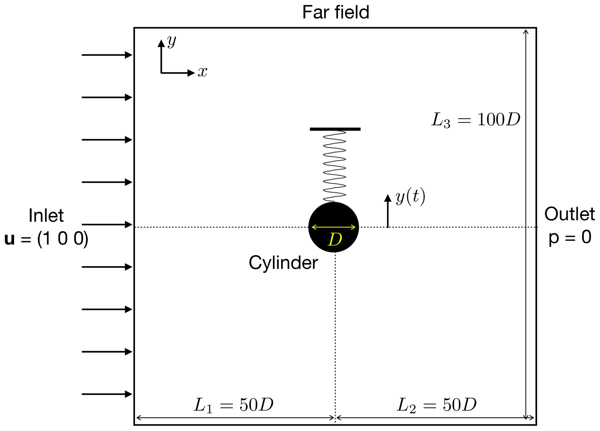
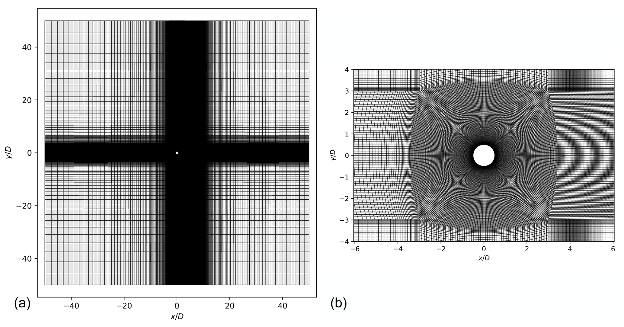
The computational domain used in the present work is sketched in Fig. 2. The cylinder is centred in a squared domain of length 50D, D being the cylinder diameter. A uniform streamwise velocity field is imposed as an initial condition and also as a Dirichlet boundary condition at the inlet of the domain. A zero-pressure Dirichlet condition is set at the outlet. The lateral far-field boundaries are set as slip walls. In this subsection, the free-vibration results are shown, whereby the dynamics of the cylinder are determined by solving Eq. (15). The domain is meshed with a structured hexahedral grid with a minimum cell height at the cylinder corresponding to , where is the friction velocity at the wall. As shown by Fig. 3, the mesh has an O-grid topology, which is commonly used for flow around cylinders. For the present laminar flow computations, the cell height at the cylinder boundary of Δy is 0.05. A mesh convergence analysis was performed and led to the conclusions that a mesh with 30 096 cells was sufficient to obtain accurate converged results. The time step size was further varied to keep the Courant–Friedrichs–Lewy (CFL) number equal to 0.7 for all the computations.
3.1.2 Free vibration
This section shows the results of a cylinder vibrating freely in the direction transverse to the flow. Here, the flow is laminar, and the results are compared with those available in the literature (Carmo et al., 2011), where a loosely coupled numerical FSI framework was also used. The simulations are conducted with a Reynolds number of Re=150, a mass ratio (L being the length of the equivalent three-dimensional cylinder), and a damping factor of ζ=0.007. The reduced velocity varies in the range of . The non-dimensional maximum amplitude of the cylinder is shown in Fig. 4 for both the present simulations and the results from the literature. The lock-in region is clearly identified for , and good agreement between the present results and the reference solution is obtained for the whole range of reduced velocities. Figure 5 shows the cylinder frequency divided by its natural frequency. Again, good agreement is obtained between the present results and the literature. As expected, the motion frequency equals the natural frequency in the lock-in region (i.e. ), whilst the frequency ratio follows the Strouhal relation outside the lock-in band. These results demonstrate that the present weakly coupled FSI model is capable of predicting the dynamics of a light cylinder undergoing VIV in laminar flow conditions.
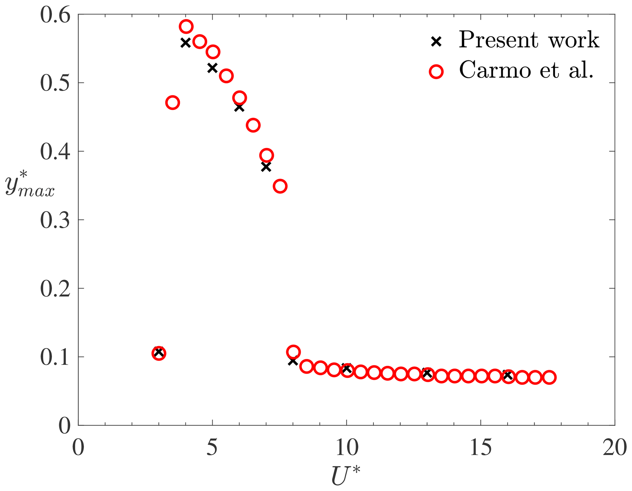
Figure 4Non-dimensional maximum motion amplitude as a function of the reduced velocity for Re=150, , and ζ=0.007.
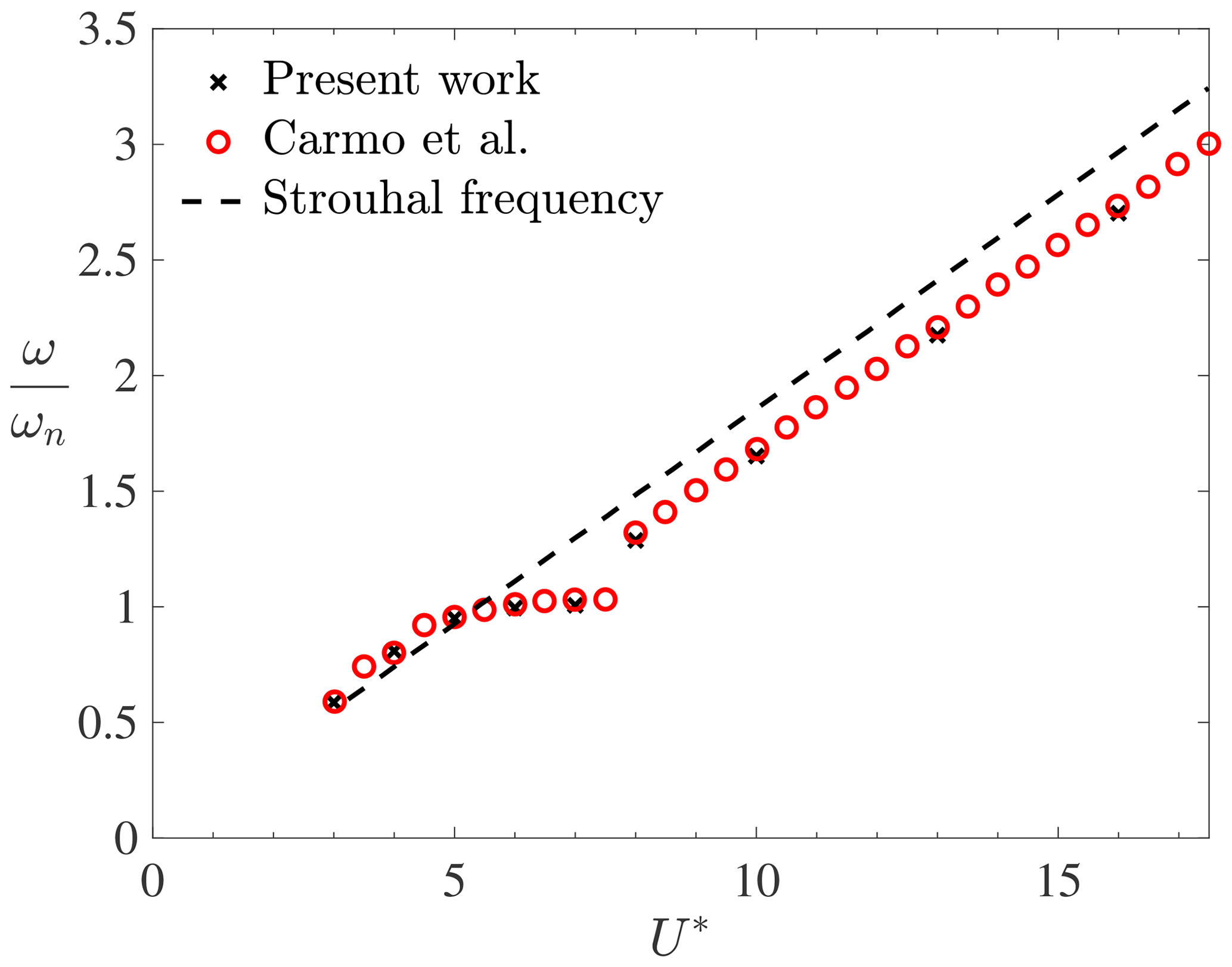
Figure 5Ratio of the motion frequency to the natural frequency as a function of the reduced velocity for Re=150, , and ζ=0.007.
3.2 Turbulent flow
In this section, the cylinder is placed in a turbulent flow as typically encountered by wind turbine towers. First, the simulation set-up is presented. Then, the simulation results are presented for three conditions: stationary cylinder, forced vibrations, and free vibrations.
3.2.1 Simulation set-up
The computational domain and boundary conditions are identical to those used in the previous subsection. However, since a turbulence model is used here, additional boundary and initial conditions are needed for the turbulent quantities. In particular, the initial value of the turbulent kinetic energy is set to
with the turbulence intensity being set at TI =0.03, and the inlet velocity is u∞=1, whilst the initial value of the turbulence-specific dissipation rate is equal to
with , μ being the fluid dynamic viscosity. The initial value of the eddy viscosity is νt=0. Regarding the boundary conditions, Dirichlet conditions are imposed on both k and ω at the inlet, with values equal to the initial ones, respectively, and Neumann conditions are imposed at the outlet. At the cylinder, the mesh is fine enough to resolve the flow up to the viscous sub-layer () using prism layers around the cylinder, with a mesh growth ratio equal to 1.2 and a minimum cell height at the cylinder equal to . Converged results were obtained for a mesh with 98 730 grid points. As for the laminar flow simulations, the maximum CFL number was kept constant at CFL =0.7. Since the viscous sub-layer is mostly laminar, the turbulent quantities are such that turbulence is suppressed at the wall. Thus, at the cylinder boundary, , νt=0, and
with β1=0.075 and ywall being the mesh cell height at the wall (Menter, 1992).
3.2.2 Flow past a stationary cylinder
Before considering flow past moving cylinders, the accuracy of the k–ω SST turbulence model in the supercritical regime is first assessed on flow past a stationary cylinder with a Reynolds number . Table 2 compares the results of the present simulations with numerical and experimental data from the literature in terms of the Strouhal number St, mean drag coefficient CD,mean, base pressure coefficient cp,b at (θ being the circumferential angle at a point on the cylinder surface starting from the stagnation point), and flow separation angle θsep. The values marked with a double asterisk are estimated indirectly based on the available pressure distribution where the constant pressure plateau is reached. Overall, it is observed that the present results agree well with the literature, especially when compared with other numerical results obtained with either URANS (Ong et al., 2009) or DES (Travin et al., 2000) turbulence models. The pressure coefficient at the cylinder surface is further plotted in Fig. 6. Again, it is clear that the present URANS results match well with the results from other numerical studies. Compared to experimental works (Achenbach, 1968; Jones et al., 1969), the present pressure coefficient agrees well in the front part of the cylinder for . For larger values of θ, the numerical results show both an earlier pressure recovery (at ) and a less pronounced negative peak for cp. It was shown by Achenbach (1968) that the transition point of the boundary layer is at for that Reynolds number. It seems that the pressure distribution starts to deviate around this point, which could indicate that the transition has an impact on the pressure distribution. The boundary layer in the experiment of Jones et al. (1969) continues to decelerate further aft (at ), which explains why the separation also occurs later in their measurements. This might indicate that the numerical models do not fully predict the detached flow accurately. This is in line with previous observations made in the literature, although with different Reynolds numbers (Ferrand et al., 2006; Catalano et al., 2003). The friction coefficient at the cylinder surface is also plotted in Fig. 7. The present numerical results agree well with other numerical studies that use either LES (Catalano et al., 2003) or DES (Travin et al., 2000). The peak of the maximum friction coefficient is slightly lower than that obtained from DES. However, the overall agreement is good, and the separation location is also accurately captured and compares well with the experiment of Achenbach (1968). The numerical values of the friction coefficient cf for are generally much higher than the experimental values. This can be explained by the fact that the numerical studies assume fully turbulent transition and therefore lead to significantly higher friction coefficient values. In particular, the overestimation is caused by the fact that the laminar flow at the beginning part of the cylinder wall is not taken into account in the numerical models. This is in line with the observations of Travin et al. (2000) and Catalano et al. (2003). Only the URANS simulations of Ong et al. (2009) show much smaller friction coefficient values. However, this study used a k–ϵ turbulence model, which is known to perform poorly with flow separation and strong pressure gradients. This could explain why these URANS results underestimate the skin friction coefficient compared to the other numerical studies. Despite the discrepancies in cp and cf between the numerical and experimental results, the present turbulence model is deemed to be adequate for the purpose of this work as it provides results that are in line with other trustworthy numerical studies in the supercritical regime.
(Ong et al., 2009)(Travin et al., 2000)(Achenbach, 1968)(Jones et al., 1969)Table 2Comparison of data for flow past a stationary cylinder in the supercritical regime. The values marked with * have been estimated indirectly based on the available pressure distribution where the constant pressure plateau was reached.
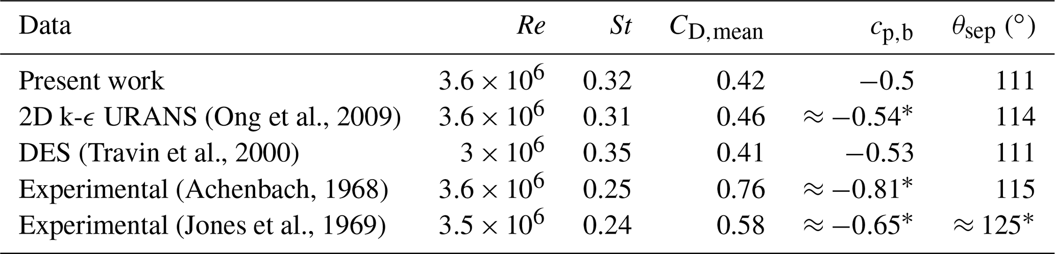
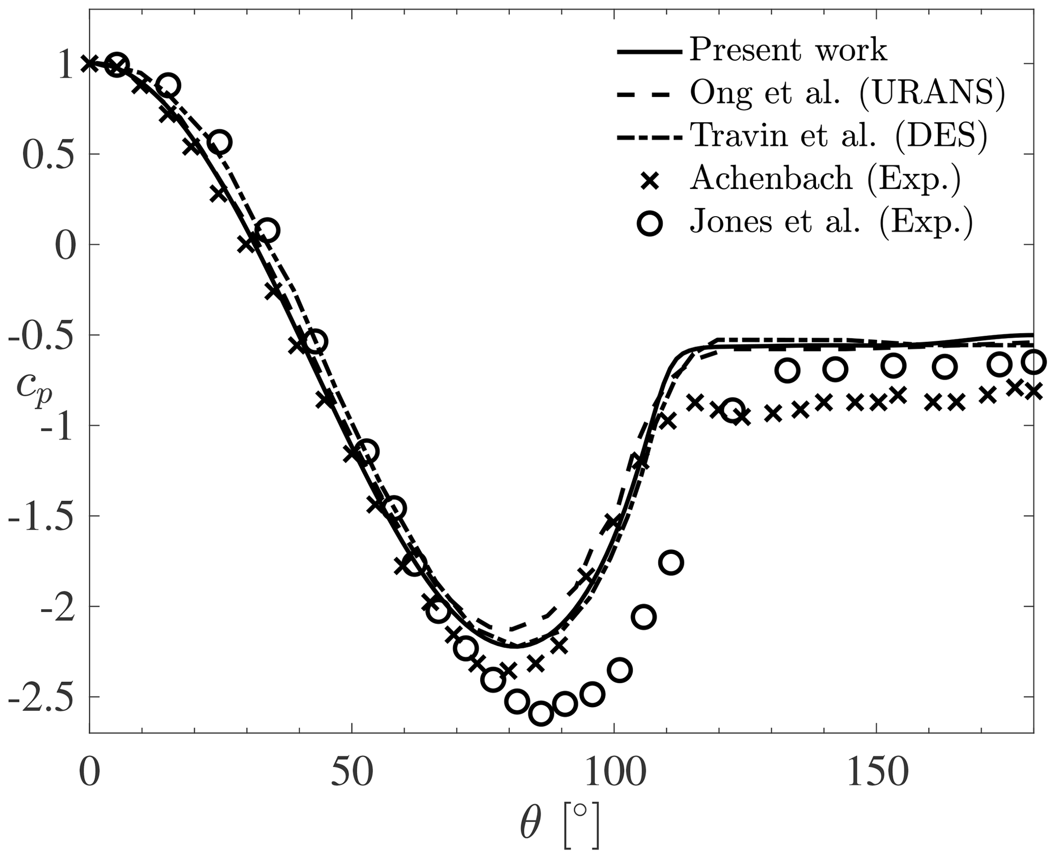
Figure 6Time-averaged pressure distribution for flow past a stationary cylinder in the supercritical turbulent regime.
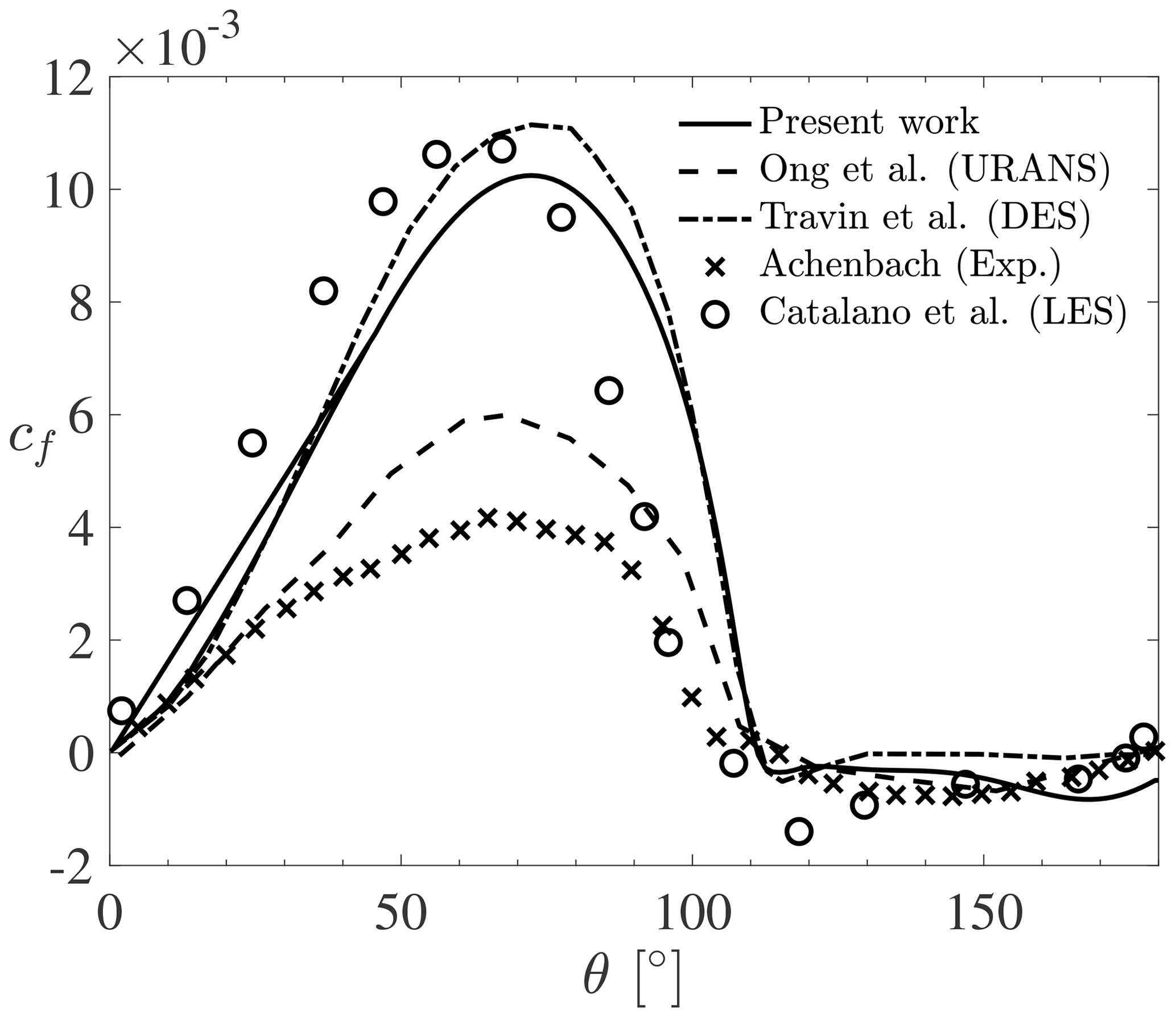
Figure 7Time-averaged friction coefficient for flow past a stationary cylinder in the supercritical turbulent regime.
3.2.3 Flow past a cylinder under forced vibration
In this section, the transverse motion of the cylinder is prescribed for different frequencies ωf. Seven different frequencies are considered, each corresponding to a different reduced velocity and Reynolds number, as indicated in Table 3. In the latter, Stf denotes the non-dimensional forcing frequency of the cylinder, while St is the Strouhal number associated with flow past a stationary cylinder with the same Reynolds number. The latter is obtained numerically with the same mesh as for the corresponding moving cases. The simulations are further run for seven different values of the prescribed maximum motion amplitude. The root mean square of the lift coefficient (non-dimensionalized by its value for a stationary cylinder) is shown in Fig. 8 for different ratios Stf∕St and prescribed motion amplitudes . As expected, the lift magnification due to the cylinder motion increases with both the non-dimensional frequencies and . The increase with frequency is rather linear except close to . The peak in lift magnification around a unitary reduced frequency is believed to be a consequence of the wake lock-in on the cylinder motion. For and , our simulation results indicate that the lift magnification becomes very large, which is believed to be due to the effective added mass of the fluid caused by the vorticity dynamics (Williamson and Govardhan, 2008).
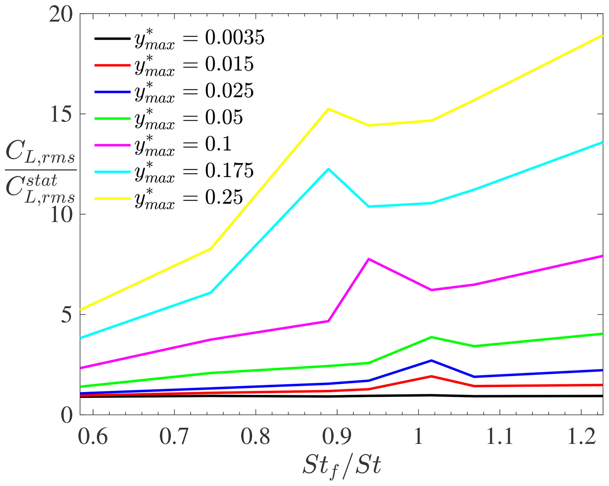
Figure 8Root mean square of the lift coefficient (non-dimensionalized by its value for a stationary cylinder) for forced vibrations in the supercritical turbulent regime with different frequency ratios Stf∕St and prescribed motion amplitudes .
Another observation is that the lock-in band width increases with increasing motion amplitudes, with a move towards lower reduced frequencies as the oscillation amplitude increases. Both these observations, namely increased lift magnification at high frequency ratios and wider lock-in band with larger motions, were observed in the experimental results obtained from NASA under similar conditions (Jones et al., 1969), as shown in Fig. 9. Although the experimental results show some scatter, a peak of lift magnification is obtained around , decreasing for slightly larger Strouhal number ratios before increasing further as (see for example the results at in Fig. 9).
Table 3Range of frequency ratios and velocities considered for the forced vibration of a cylinder in the supercritical regime.
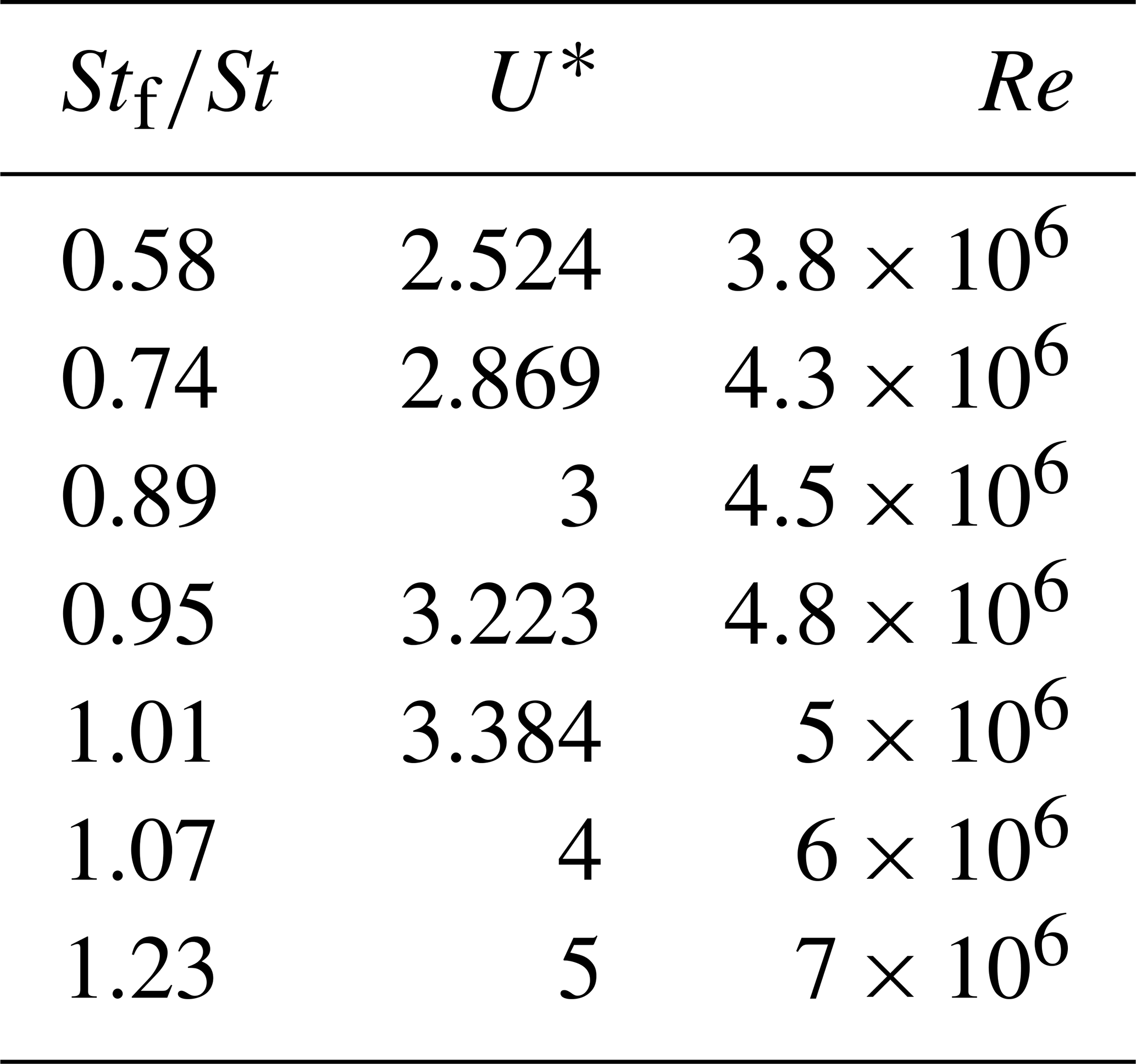
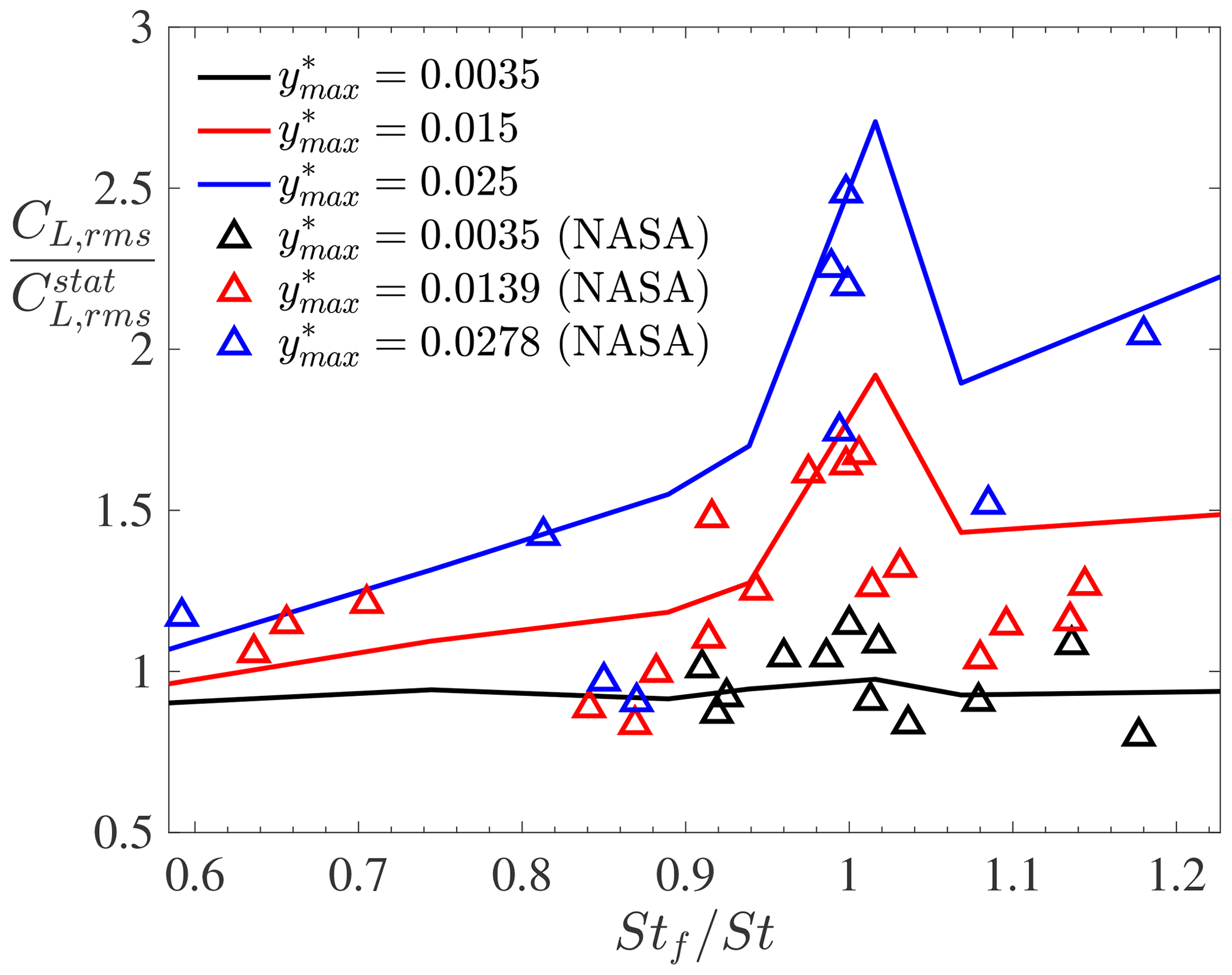
Figure 9Root mean square of the lift coefficient (non-dimensionalized by its value for a stationary cylinder) for forced vibrations compared with NASA experimental data (Jones et al., 1969) at three values of the prescribed motion amplitude.
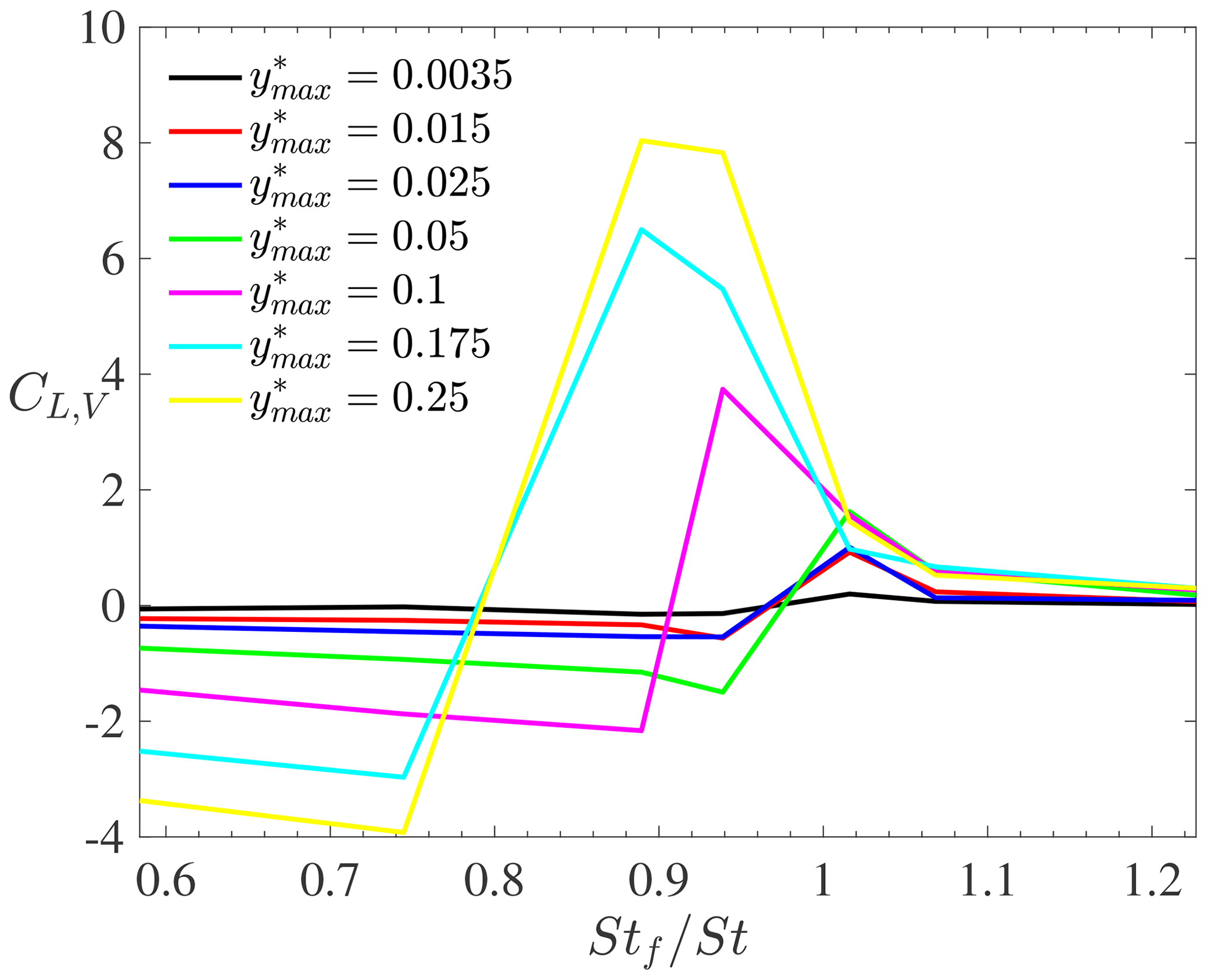
Figure 10Aerodynamic damping for forced vibrations in the supercritical turbulent regime with different frequency ratios Stf∕St and prescribed motion amplitudes .
Although the cylinder motion is prescribed, it is interesting to look in more detail at the feedback mechanism between the cylinder and the fluid motions. In order to do this, the aerodynamic damping is analysed. It is defined as the part of the harmonic lift force that is in phase with the cylinder velocity. There are different ways to compute this damping. Here, an approach based on the time-averaged energy transfer between fluid and vibrating cylinder is considered (Bourguet et al., 2011; Gopalakrishnan, 1993) as it is believed to be accurate when signals exhibit multiple frequencies. This leads to the following expression for the aerodynamic damping:
where denotes the lift coefficient, a prime denotes the fluctuating part of a quantity, and an overline denotes its time average. The aerodynamic damping is plotted for the different simulation cases in Fig. 10. For , it is observed that CL,V increases with the motion amplitude. This indicates that the wake dynamics tend to oppose the cylinder motion as the latter increases, hence stabilizing the system. By contrast, for , the aerodynamic damping is negative, with an absolute value increasing as the cylinder displacement increases. In that case, the wake dynamics tend to further amplify the system motion, hence leading to an unstable system behaviour. In the lock-in band, for , the nature of the interaction between fluid and structural motion depends on the amplitude of the prescribed motion. However, a stabilizing fluid–structure interaction behaviour is observed for large motion amplitudes. These observations agree with those obtained from Jones et al. (1969). In particular, the overall behaviour of the experimental aerodynamic damping in the supercritical turbulent regime for varying frequency ratios was found to be similar to the present CFD results.

Figure 11Non-dimensional maximum motion amplitude as a function of the reduced velocity for , ζ=0.003, and . Insets show the time evolution of the lift coefficient at certain values of reduced velocities.
3.2.4 Flow past a freely vibrating cylinder
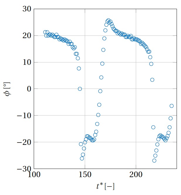
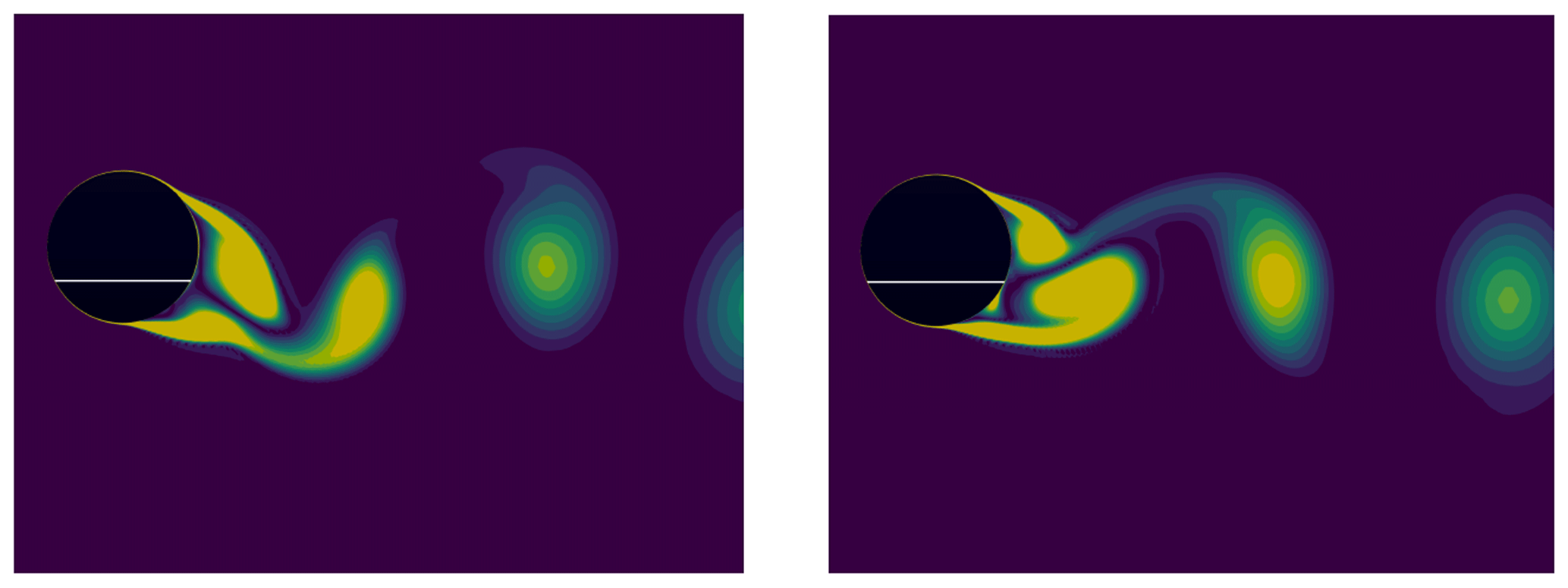
In this section, the cylinder is left to freely vibrate under the vortex-induced vibrations. The results are shown for a baseline value of mass ratio and damping coefficient ζ=0.003, which are representative of a realistic wind turbine tower. The effect of these values on the results is also briefly discussed in this section. The reduced velocity is varied from to , corresponding to Reynolds numbers between and , respectively. The associated non-dimensional maximum motion amplitude under these conditions is shown in Fig. 11, in which the lock-in band can be clearly visualized. Additionally, the insets show the time evolution of the lift coefficient on the cylinder for certain values of reduced velocity. The associated values of reduced frequency, , are also shown for each inset. These insets illustrate that for some values of U*, a non-harmonic lift response (and consequently also motion response) is obtained. Outside the lock-in region, at low values of U*, the vortex-shedding frequency is dominated by the stationary Strouhal relation and is very different from the natural frequency of the cylinder. This is also apparent from Fig. 12. In that case, the mean aerodynamic forces are similar to those of a stationary cylinder, and little cylinder motion is observed. Furthermore, the vorticity contours in the cylinder wake follow a 2S pattern similar to flow past a stationary cylinder. Furthermore, the phase angle ϕ between the lift force and the transverse displacement is constant and equals 0∘. When U* increases to values close to the lock-in band, the time histories of the aerodynamic forces and cylinder motion change. First, the cylinder displacement increases substantially because the vortex-shedding frequency gets closer to the natural frequency of the cylinder. Second, the cylinder motion shows two main frequency responses instead of one. The dominant frequency in the time evolutions of the lift and motion amplitude still equals the Strouhal frequency. However, performing a power spectral density on these time signals shows that a second (much smaller) frequency peak coincides with the natural frequency. This explains the observed increase in cylinder motion compared to cases at smaller reduced velocities. The phase angle between lift force and transverse displacement is also different than for smaller values of U*. Instead of being constant, it periodically oscillates in time around a mean value of . When the phase angle is larger than the mean value, the aerodynamic damping decreases, and the fluid amplifies the cylinder excitation. By contrast, when the phase angle is smaller than the mean value, the fluid damps the cylinder motion. When U* is increased further inside the lock-in band, the time histories of the lift and displacement also show two frequencies. However, the dominant peak corresponds to the natural frequency of the cylinder, hence confirming that the wake behaviour becomes driven by the cylinder oscillations rather than the Strouhal relation. Furthermore, the lift force (and also motion displacement) alternates between growth and decay, which also corresponds to a change in sign of the aerodynamic damping. In particular, when the lift force increases, the fluid dynamics excite the cylinder. By contrast, when the lift force decreases, the fluid dynamics damp the cylinder motion. In doing so, the vortex-induced vibrations continuously alternate between self-exciting and self-limiting behaviours. This alternation can also be related to a drop in phase angle between lift force and cylinder displacement. Figure 13 shows the time evolution of the phase angle for . It is apparent that the phase angle changes sign as time evolves. When ϕ>0, the fluid excites the cylinder motion, and the magnitude of both the lift force and the transverse displacement increases. By contrast, when ϕ<0, the lift force lags behind the displacement, and the fluid dampens the cylinder motion. The magnitude of both the lift force and the cylinder displacement also decreases. The phase angle drop can also be related to the wake pattern development as shown in Fig. 14. The left figure corresponds to a positive phase angle at , while the right figure is taken at , when the phase angle is negative. When the phase angle is positive, the vortices are shed from the bottom side of the cylinder when the cylinder reaches its maximum positive displacement. The opposite is true when the phase angle switches sign. In that case, the vortices are shed from the same side as where the cylinder is oscillating to. It seems that when the cylinder motion becomes too large, the wake reorganizes itself in such a way that it starts damping the cylinder motion. The self-exciting behaviour becomes a self-limiting behaviour. This alternation of behaviours is influenced by both the mass ratio and the damping factor. If the mass ratio is reduced, the non-dimensional displacement amplitude increases. This is expected as a lower mass ratio leads to a lower structural inertia when compared to the fluid inertia. This makes the cylinder more susceptible to oscillations and possibly lock-in. By contrast, for very large mass ratios, the cylinder motion decreases and eventually tends to a stationary cylinder. There is thus a critical value of the mass ratio at which the system stops undergoing enhanced fluid–structure interactions. Non-harmonic behaviours of the lift and motion displacement are also less likely to occur at large mass ratios and large damping factors because the larger structural inertia prevents the cylinder from changing to a different dynamic state. When U* is increased further, in a certain range, the lift force, drag force, and transverse displacement do not show a clear converged pattern (see inset in Fig. 11 at ). It is not excluded that, if the simulation were run for even longer times, a self-limiting behaviour could appear. However, the observed behaviour is believed to have physical causes rather than being a numerical artefact. This is because the operation points for which this happens correspond to reduced frequencies between 0.5 and 0.7, for which the results of the forced-vibration cases led to unstable behaviours. By contrast, at smaller values of U*, the reduced frequencies are large (), and a stable forced-vibration behaviour was obtained. It is also worth noting that the large lock-in band observed in the present study is in line with previous observations made in the literature under similar conditions. For example, Guilmineau and Queutey (2004) and Assi (2009) showed large values of non-dimensional displacement for reduced frequencies as low as , whilst the wind tunnel experiment of Feng (1968) also showed a lock-in region extending to reduced frequencies of .

Figure 12Ratio of the motion frequency to the natural frequency as a function of the reduced velocity for , ζ=0.003, and .
In this work, numerical simulations of a two-dimensional cylinder undergoing vortex-induced vibrations were performed. First, the fluid–structure interaction methodology was validated in the laminar regime, for which direct numerical simulations (DNSs) were able to reproduce results from the literature. Second, supercritical turbulent regimes experienced by wind turbine towers were simulated using the k–ω SST unsteady Reynolds-averaged Navier–Stokes (URANS) model. The ability of our model to simulate flow past a stationary cylinder in the turbulent supercritical regime was demonstrated by comparing the present results with other URANS, large-eddy simulations (LESs), detached-eddy simulations (DESs), and experimental results from the literature. Additionally, the present tools were capable of simulating the dynamic behaviour of the cylinder (including lock-in) for a range of reduced velocities and Reynolds numbers. In particular, good agreement was found between the present results and those obtained from wind tunnel experiments under forced vibrations. When the cylinder was left free to oscillate under the effect of vortex shedding, the results highlighted a complex interplay between structural and fluid dynamics for values of reduced velocity close to or inside the lock-in band. In particular, there was a continuous alternation between self-exciting and self-limiting vortex-induced vibrations. The physical feasibility of this interplay was supported by both the role of the aerodynamic damping, which was shown to continuously change sign at these operating points, and the results from forced-vibration oscillations under similar conditions.
Traditionally, the designs of wind turbine towers are soft-stiff, with the tower's natural frequency being larger than the rotor's rotational frequency but smaller than the blade's passing frequency. Today, advanced wind turbine controllers can work through resonance conditions, allowing the tower's natural frequencies to overlap with the rotor's rotational frequency and the blade's passing frequency. This makes soft-soft designs possible, which is promising to enable a significant reduction in tower mass when the tower height is larger than 100 m (Dykes et al., 2018). During the installation phase of wind turbines, however, the rotor–nacelle assembly is absent, and wind turbine controllers cannot be used to damp vibrations. This is the case during the whole installation cycle of jackets and monopile foundations as well as their vertical storage and transport. During that time, towers might stand without rotors for several weeks. They act as a clamped beam and are subjected to supercritical Reynolds numbers. Over the past years, the tower-clamped first-mode frequency has been reduced, and this trend is continuing. This means that both the combined first eigenmodes and the second mode of vibration can interact with the wind climate and become critical for the dynamics of the structure and VIVs. The present work shows that, in the supercritical flow regime, a cylinder can experience episodes of sustained VIV, where the Strouhal relation is not valid. This means that the best mitigation strategy is to have a robust damping mechanism that is effective for the range of critical first bending frequencies. This work presents some limitations that should be addressed in future studies. For example, future work should look at three-dimensional tower sections as well as the influence of non-uniform wind flows on the present results. Although this has already been partly investigated in the literature, there is a lack of analyses for the supercritical regime. Furthermore, the use of a tapered cylinder instead of a circular one is expected to lower the risk of VIVs and move the lock-in region to lower reduced velocities. Nevertheless, circular cylinders are very relevant to new wind turbine tower designs as some manufacturers are currently looking into having minimal taper at the top sections. Finally, during the installation phase, wind turbine towers are usually transported in groups. Therefore, wake–tower interactions and their effect on the development of VIVs should be further investigated.
The data was generated with the open-source code OpenFOAM-v1812, available at: https://www.openfoam.com/releases/openfoam-v1812/ (Heather, 2018).
The data published in the paper are accessible at the following DOI: https://doi.org/10.4121/uuid:33f213fe-df8e-4b71-bec5-feada4e12a6d (Derksen et al., 2020).
AV: paper writing, results post-processing, interpretation of results, responsible supervisor of the work. AD: model setup, results generation, results post-processing, interpretation of results. MF: support with model setup, results generation and post-processing. KS: industrial supervisor of the work, interpretation of results, some text editing.
The authors declare that they have no conflict of interest.
The opinions expressed in this document reflect only the authors' view and in no way reflect the European Commission's opinions. The European Commission is not responsible for any use that may be made of the information it contains.
This article is part of the special issue “Wind Energy Science Conference 2019”. It is a result of the Wind Energy Science Conference 2019, Cork, Ireland, 17–20 June 2019.
The authors are grateful to the European Commission for the financial support as well as to Siemens Gamesa Renewable Energy for their insights into wind turbine tower designs and working conditions.
This research has been supported by the European Union's Horizon 2020 research and innovation programme (project STEP4WIND, grant agreement no. 860737) and the AWESCO project (grant agreement no. 642682).
This paper was edited by Katherine Dykes and reviewed by two anonymous referees.
Achenbach, E.: Distribution of local pressure and skin friction around a circular cylinder in cross-flow up to , J. Fluid Mech., 34, 625–639, 1968. a, b, c, d, e
Assi, G.: Mechanisms for flow-induced vibration of interfering bluff bodies, PhD thesis, Imperial College London, London, UK, 2009. a
Balasubramanian, S., Haan, F., Szewczyk, A., and Skop, R.: An experimental investigation of the vortex-excited vibrations of pivoted tapered circular cylinders in uniform and shear flow, J. Wind Eng. Ind. Aerodyn., 89, 757–784, 2001. a
Belloli, M., Giappino, S., Muggiasca, S., and Zasso, A.: Force and wake analysis on a single circular cylinder subjected to vortex induced vibrations at high mass ratio and high Reynolds number, J. Wind Eng. Ind. Aerodyn., 103, 96–106, 2012. a
Bourguet, R. and Triantafyllou, M.: The onset of vortex-induced vibrations of a flexible cylinder at large inclination angle, J. Fluid Mech., 809, 111–134, 2016. a
Bourguet, R., Karniadakis, G., and Triantafyllou, M.: Lock-in of the vortex-induced vibrations of a long tensioned beam in shear flow, J. Fluids Struct., 27, 838–847, 2011. a
Bourguet, R., Karniadakis, G., and Triantafyllou, M.: Distributed lock-in drives broadband vortex-induced vibrations of a long flexible cylinder in shear flow, J. Fluid Mech., 717, 361–375, 2013. a
Breuer, M.: A challenging test case for large eddy simulation: high Reynolds number circular cylinder flow, Int. J. Heat Fluid Flow, 21, 648–654, 2000. a
Brika, D. and Laneville, A.: Vortex induced vibrations of a long flexible circular cylinder, J. Fluid Mech., 320, 117–137, 1993. a
Carmo, B., Sherwin, S., Bearman, P., and Willden, R.: Flow-induced vibration of a circular cylinder subjected to wake interference at low Reynolds number, J. Fluids Struct., 27, 503–522, 2011. a
Catalano, P., Wang, M., Iaccarino, G., and Moin, P.: Numerical simulation of the flow around a circular cylinder at high Reynolds numbers, Int. J. Heat Fluid Flow, 24, 463–469, 2003. a, b, c, d, e
Derksen, A.: Numerical simulation of a forced and freely-vibrating cylinder at supercritical Reynolds numbers, MS thesis, TU Delft and Siemens, Delft, the Netherlands, 2019. a, b, c, d
Derksen, A., Viré, A., Folkersma, M., and Sarwar, K.: Data underlying the research of: Two-dimensional numerical simulations of vortex-induced vibrations for a cylinder in conditions representative of wind turbine towers, 4TU.Centre for Research Data, https://doi.org/10.4121/uuid:33f213fe-df8e-4b71-bec5-feada4e12a6d, 2020. a, b
Dullweber, A., Leimkuhler, B., and Mclachlan, R.: Symplectic splitting methods for rigid body molecular dynamics, J. Chem. Phys., 107, 5840–5851, 1997. a
Dykes, K., Damiani, R., Roberts, O., and Lantz, E.: Analysis of Ideal Towers for Tall Wind Applications: Preprint, Tech. Rep. NREL/CP-5000-70642, National Renewable Energy Laboratory, USA, 2018. a, b
Feng, C.: The measurement of vortex-induced effects in flow past stationary and oscillating circular D-section cylinders, PhD thesis, The University of British Columbia, 1968. a, b
Ferrand, P., Boudet, J., Caro, J., Aubert, S., and Rambeau, C.: Unsteady Aerodynamics, Aeroacoustics and Aeroelasticity of Turbomachines, chap. Analyses of URANS and LES capabilities to predict vortex shedding for rods and turbines, Springer, 381–392, 2006. a
Gopalakrishnan, R.: Vortex-induced forces on oscillating bluff cylinders, PhD thesis, Massachusetts Institute of Technology, USA, 1993. a
Govardghan, C. and Williamson, C.: Modes of vortex formation and frequency response of a freely vibrating cylinder, J. Fluid Mech., 420, 85–130, 2000. a
Govardghan, C. and Williamson, C.: Defining the `modified Griffin plot' in vortex-induced vibrations: revealing the effect of Reynolds number using controlled damping, J. Fluid Mech., 560, 147–180, 2006. a
Griffin, O.: Vortex-excited cross-flow vibrations of a single cylindrical tube, ASME Journal Pressure Vessel Technology, 102, 158–166, 1980. a
Guilmineau, E. and Queutey, P.: Numerical simulation of vortex-induced vibration of a circular cylinder with low mass-damping in a turbulent flow, J. Fluids Struct., 19, 449–466, 2004. a
Heather, A., Janssens, M., Ferraris, S., Olesen, M., Sonakar, P., Ghildiyal, P., Almenar, R., Forman, M., Vilfayeau, S., Mandapathil Baby, S. Wala, M., Vo, S., Bercin, K., Kettle, K., and Mendonca, F.: OpenCFD Release OpenFOAM v1812, available at: available at: https://www.openfoam.com/releases/openfoam-v1812/, 2018. a
Heinz, J., Sorensen, N., Zahle, F., and Skrzypinski, W.: Vortex-induced vibrations on a modern wind turbine blade, Wind Energ., 19, 2041–2051, 2016. a
Horcas, S., Madsen, M., Sorensen, N., and Zahle, F.: Recent advances in CFD for wind and tidal offshore turbines, chap. Suppressing vortex induced vibrations of wind turbine blades with flaps, Springer, Switzerland, 2019. a
Hover, F., Techet, A., and Triantafyllou, M.: Forces on oscillating uniform and tapered cylinders in crossflow, J. Fluid Mech., 363, 97–114, 1998. a
Jones, G., Cincotta, J., and Walker, R.: Aerodynamic Forces on a Stationary and Oscillating Circular Cylinder at High Reynolds Numbers, Technical report TR R-300, NASA, 1969. a, b, c, d, e, f, g, h
Livanos, D.: Investigation of Vortex Induced Vibrations on Wind Turbine Towers, MS thesis, TU Delft and Siemens, 2018. a
Menter, F.: Improved two-equation k-omega turbulence models for aerodynamic flows, Technical Memorandum 103978, NASA, 1992. a
Menter, F.: Two-equation eddy-viscosity turbulence models for engineering applications, AIAA J., 32, 1598–1605, 1994. a
Menter, F. and Esch, T.: Elements of industrial heat transfer prediction, in: Proceedings of the 16th Brazilian Congress of Mechanical Engineering (COBEM), 117–127, 2001. a
Menter, F., Kuntz, M., and Langtry, R.: Ten Years of Industrial Experience with the SST Turbulence Model, in: The Fourth International Symposium on Turbulence, Heat and Mass Tranfer, 4, 625–632, 2003. a
Newmark, N.: A method of computation for structural dynamics, J. Eng. Mech., 85, 67—94, 1959. a
Ong, M., Utnes, T., Holmedal, L., Myrhaug, D., and Pettersen, B.: Numerical simulation of flow around a smooth circular cylinder at very high Reynolds numbers, Mar. Struct., 22, 142–153, 2009. a, b, c, d, e
Rosetti, G., Vaz, G., and Fujarra, A.: URANS Calculations for Smooth Circular Cylinder Flow in a Wide Range of Reynolds Numbers: Solution Verification and Validation, J. Fluid. Eng., 134, 1–18, 2012. a, b
Roshko, A.: Experiments on the flow past a circular cylinder at very high Reynolds number, J. Fluid Mech., 10, 345–356, 1961. a
Schewe, G.: On the force fluctuations acting on a circular cylinder in crossflow from subcritical up to transcritical Reynolds numbers, J. Fluid. Mech., 133, 265–285, 1983. a
Singh, S. and Mittal, S.: Flow past a cylinder: shear layer instability and drag crisis, Int. J. Numer. Meth. Fluids, 47, 75–98, 2005. a
Squires, K., Krishnan, V., and Forsythe, J.: Prediction of the flow over a circular cylinder at high Reynolds number using detached-eddy simulation, J. Wind Eng. Ind. Aerodyn., 96, 1528–1536, 2008. a
Travin, A., Shur, M., Strelets, M., and Spalart, P.: Detached-Eddy Simulations Past a Circular Cylinder, Flow, Turbulence and Combustion, 63, 293–313, 2000. a, b, c, d, e, f
van Nunen, J.: Pressure and forces on a circular cylinder in a cross flow at high Reynolds numbers, Flow Induced Structural Vibrations, pp. 748–754, 1974. a
Williamson, C. and Govardhan, R.: A brief review of recent results in vortex-induced vibrations, J. Wind Eng. Ind. Aerodyn., 96, 713–735, 2008. a