the Creative Commons Attribution 4.0 License.
the Creative Commons Attribution 4.0 License.
 | 18 Jan 2021
Model-free estimation of available power using deep learning
Albert Meseguer Urbán
Jaime Liew
Alan Wai Hou Lio
In order to assess the level of power reserves during down-regulation, the available power of a wind turbine needs to be estimated. The current practice in available power estimation is heavily dependent on the pre-defined performance parameters of the turbine and the curtailment strategy followed. This paper proposes a single-input model-free approach dynamic estimation of the available power using recurrent neural networks. Accordingly, it combines wind turbine control considerations and modern forecasting methodologies for a model-free, single-input estimation of available power. It enables a robust real-time implementation of dynamic delta control, as well as higher-accuracy provision of the reserves to the system operators.
The model-free approach requires only 1 Hz wind speed measurements as input and estimates 1 Hz available power as output. The neural network is trained, tested and validated using the DTU 10 MW reference wind turbine HAWC2 model under realistic atmospheric conditions. The unsteady patterns in the turbulent flow are represented via long short-term memory (LSTM) neurons which are trained during a period of normal operation. The adaptability of the network to changing inflow conditions is ensured via transfer learning, where the last LSTM layer is updated using new measurements. It is seen that the sensitivity of the networks to changing wind speed is much higher than that of turbulence, and the updates are to be implemented solely based on the altering inflow velocity. The validation of the trained LSTM networks on time series with 7, 9 and 11 m s−1 mean wind speeds demonstrates high accuracy (less than 1 % bias) and capability of transfer-learning online. Including highly turbulent inflow cases, the networks have shown to comply with the most recent grid codes, which require the quality of the available power estimations to be evaluated with high accuracy (less than 3.3 % standard deviation of the error around zero bias) at 1 min intervals.
- Article
(3102 KB) - Full-text XML
- BibTeX
- EndNote


As the share of wind energy increases in power systems around the world, new challenges regarding the control and operations of wind power plants are encountered. In order to maintain power system stability, transmission system operators (TSOs) are developing new grid codes requiring contributions not only from conventional generators, but also from wind power plants, globally. In this context, here we focus on the active power contribution of wind turbines to provide frequency support and power reserves via down-regulation (also referred to as curtailment, de-rating or de-loading).
The curtailment of wind turbines can be implemented both as balance control, where the turbine power output is reduced to a constant value, and as delta control, where the output is reduced by a certain percentage of the available power (Attya et al., 2018; Fleming et al., 2016; Hansen et al., 2006). Additionally, the active power reduction for both strategies can be achieved by adjusting the rotor blade pitch angles and/or operating at a sub-optimal rotor speed compared to the maximum energy capture value (Wilches-Bernal et al., 2016). Although modern turbines are capable of implementing both balance and delta control, due to the uncertainties in the estimated available power (Göçmen et al., 2016; Göçmen and Giebel, 2018; Göçmen et al., 2019; Pinson, 2006; Pinson et al., 2007), balance control is the preferred industrial application as its set point is independent of the available power (Kristoffersen, 2005). The amount of power reserves however, which is defined as the difference between the available and the produced power under curtailed operation, does depend on the available power in the wind for both delta and balance control. This is particularly critical for compensation schemes under mandatory down-regulation, as well as (existing and expected) flexible balancing market structures, where the reserve power is traded at different timescales depending on the regional balancing market schemes (Chinmoy et al., 2019).
Generally, trading in the electricity markets is performed in advance with a given forecast horizon. Depending on the bidding structure, the available power production of an asset is to be predicted sometimes as shortly as 5 min ahead (e.g. Rana and Koprinska, 2016). The forecasting tools can be based on physical or statistical modelling, as well as the combination of both. Many perform post-processing via model output statistics to reduce the remaining error. Some approaches focus on the best possible estimate of the local wind speed while some directly extract the wind power generation potential. Statistical models use explanatory variables and historical/online information (measurements, log-data, etc.), generally implementing recursive techniques, such as recursive least-squares or artificial neural networks (or deep learning) (Wang et al., 2016). In fact, forecasting is the field with the most deep-learning (and broadly artificial intelligence) applications in wind energy, e.g. Ghaderi et al. (2017), Chen et al. (2018) and Mujeeb et al. (2019). For a recent review on deep-learning-based wind speed forecasting for several forecast horizons, see Bali et al. (2019). However, while forecasting the available power, the operational status and potential effects of control scenarios are often overlooked, especially for higher (than e.g. 5 min) frequencies at a single turbine level.
For the operational considerations and higher-frequency system stability issues, the timescales considered in the market-based forecasting are already long-term ahead. In order for the balancing responsible parties to be compensated for during mandatory down-regulation by the TSOs, wind power plants are expected to provide information regarding their power production on much shorter timescales. As stated in the recent grid requirements in Germany (50Hertz, Amprion, Tennet, TransnetBW, 2016), the available power is to be calculated for 60 s intervals for down-regulated wind farms. Additionally, the 1 min standard deviation of the percentage error of the available power is required to be less than ±3.3 % (after the pilot phase). The enforced regulations are difficult to comply with and are subject to penalty if not met.
The current practice in available power estimation is to assess the incoming wind speed to derive the possible power output of the turbine via optimum performance curve. One of the most common approaches to approximate the (effective) wind speed is by solving the static wind power equation, which is widely adopted in the wind turbine industry as well as the wind research community (e.g. van der Hooft and van Engelen, 2004; Göçmen et al., 2014). More details on the approach are provided in Sect. 2. Ma et al. (1995) demonstrate that directly mapping the static relation does not give satisfactory performance and concludes that the inclusion of dynamic models can significantly improve the wind speed estimate. Thus, an increasing number of studies (e.g. Østergaard et al., 2007; Meng et al., 2016) began to utilize observer theory, in particular, Kalman filtering. For example, in Østergaard et al. (2007), the aerodynamic torque is considered a system disturbance state, and it is estimated by the use of an observer-based system on a simple drivetrain model with pre-defined dynamics for the aerodynamic torque. Subsequently, the calculation of the wind speed is done by inversion of the static mapping between the aerodynamic torque and wind speed. One of the drawbacks of searching through the static relation, to find the wind speed estimate, is its computational cost, where a Newton–Raphson method is often employed to find the corresponding wind speed given the turbine measurement on a discrete power coefficient CP of surface. On the other hand, some methods do not require the use of iterative gradient methods, for example, by considering the wind speed directly as a state to the system, and such a wind state can be estimated via an observer Kalman filter. In Selvam (2007), the wind dynamics are modelled as a random walk and augmented with a linear turbine model including a simple drivetrain and tower dynamic model. A linear Kalman filter is then employed to estimate the wind speed for feed-forward control purpose. Similar techniques have also been utilized in Stol and Balas (2003) and Simley and Pao (2016). A study by Knudsen et al. (2011) employed a non-linear turbine model including simple drivetrain, tower and wind speed dynamics where the effective wind speed is estimated by an extended Kalman filter. Similar methods are also reported in Henriksen et al. (2012), where the dynamic inflow model is included. Besides the Kalman-filter-based approaches, some studies (Ortega et al., 2011, 2013) used a more advanced state estimation technique of immersion and invariance to construct a wind speed estimation with proof of global convergence under certain assumptions. For more details and further information on wind speed estimation, see Soltani et al. (2013) and references therein.
The state-of-the-art available power estimation is highly dependent on the considered turbine models, as well as the operation strategy for curtailment. More specifically, the majority of the methods rely on the pre-calculated power coefficient, CP, or the certified nominal power curve to convert (rotor-effective) wind speed to (available) power. However, the varying wind speed and turbulence levels activate different dynamics within the turbine structure and cause different control responses (Murcia et al., 2018). In addition, temporally and spatially local characteristics of the flow (e.g. humidity, temperature) and the condition of the turbine (e.g. blade erosion, dust, component wear or failure) highly affect the CP and the power curve behaviour. Therefore, these generally deterministic approaches fail to represent the detailed dynamics required to produce high-frequency available power signal accurately (Jin and Tian, 2010), and they are an important source of uncertainty (Lange, 2005). In order to tackle the inadequacy of the turbine models to fully represent the dynamic power output of a turbine under turbulent inflow, a model-free approach to transfer the wind speed to power is a strong alternative.
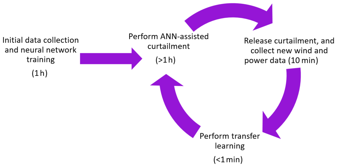
Therefore in this study, the aim is to consider the wind turbine generator (WTG) control and modern forecasting methodologies for a model-free, single-input estimation of available power. It enables a robust real-time implementation of dynamic delta control, as well as the provision of the reserves to the system level within the frame of (strictest) European grid regulations. In the model-free estimation of available power, the unsteady patterns in the turbulent flow are represented via long short-term memory (LSTM) neurons (Hochreiter and Schmidhuber, 1997), which is a special building unit for recurrent neural networks (RNNs). The proposed method for integrating an LSTM network in a curtailment strategy is outlined in Fig. 1. During a period of normal operation of a WTG, wind speed and power output time series data are collected for at least an hour to establish a training dataset. Next, the network is trained on the collected data which, depending on the available processing power, can be performed within seconds. Accordingly, the wind turbine operator can announce its participation in the reserve market online or ahead of time with the intention of performing delta or balance control for curtailment. Down-regulation is then performed using the LSTM predictor which provides the set point based on the available power. The model-free estimation approach can be rapidly retrained with newly collected data using transfer learning, where the last LSTM layer of the network is updated using the new information.
The synthetic time series used in this study is generated using the DTU 10 MW reference wind turbine (Bak et al., 2013) with the aeroelastic code HAWC2 (Bak et al., 2012) under realistic atmospheric conditions, and the simulation results are publicly available1. First, the sensitivity of the state-of-the-art available power predictions to the curtailment operation strategy is briefly discussed and quantified in Sect. 2. To address the issue, a detailed analysis of LSTM neural networks and the potential of transfer learning to adapt to changing inflow conditions is presented throughout Sect. 3. This research focus is highly important for the individual turbine control and its role in the power system stability, as well as the business case of wind energy in the existing and upcoming market scenarios.
As stated earlier, current methods for estimating available power typically make use of pre-defined power curves or power coefficient calculations. Here in this section, we discuss the assessment of wind speed and the sensitivity of the model-dependent approaches to the implemented curtailment strategy.
Point measurements of the wind speed using, for example, cup or sonic anemometers, are often unreliable at estimating the potential power production of a wind turbine as the spatial variations in the wind field are not captured. For example, a naive approach at estimating available power is
where the air density, ρ; rotor radius, R; and power coefficient, CP, are assumed to be constant with variable (effective) wind speed, U. Equation (1) presents a number of weaknesses, namely the inability to capture the dynamic response of the wind turbine to changing wind speeds, or the spatial variations in the wind field. For this reason, the rotor effective wind speed, which is defined as the spatial average wind speed over the rotor plane, is preferred in terms of power estimation. Although there are numerous methods for estimating rotor effective wind speed, the majority of methods use operating data of the wind turbine to create the estimate (Jena and Rajendran, 2015). A simple strategy is to estimate the wind speed for a given power output using a polynomial fit (Thiringer and Petersson, 2005). This method can be extended by including the rotor speed and blade pitch angle in conjunction with a CP look-up table to infer the wind speed as shown in Bhowmik et al. (1998). For derated operation, these methods are problematic as the dependency between the wind speed and a turbine's operating points varies based on the desired level of down-regulation. The use of a predefined CP curve to estimate available power therefore becomes unreliable. However, state space approaches where the convergence of the wind estimation error is analysed systematically can potentially respond to that problem.
There are several benefits of formulating a wind speed estimation as a system state estimation problem compared to methods that use static relation mapping the power or aerodynamic torque to wind speed. For example, a substantial body of mature and sophisticated state estimation theory can immediately be brought to bear upon the design of the wind estimator. Moreover, in an observer design where the wind speed is considered a system state, the use of slow gradient methods for solving the static relations can be avoided, resulting in better computational speed and a smooth wind speed estimate.
Typically, to formulate a state estimation problem, a simplified model of the non-linear dynamics is required that needs to capture the key dynamics of the turbine. For brevity, a widely used non-linear turbine system model is employed, including the dynamics of rotor drivetrain, tower and wind speed (see Knudsen et al., 2011; Lio et al., 2019):
where xk=[ωk, , xfa,k, is the system state vector at the sample time k∈ℤ containing the rotor speed, fore-aft velocity and displacement of the tower-top and ambient wind speed, whilst the system input , contains the generator torque and pitch angle, and yk=[ωk, , denotes the system output. The state transition and output functions are denoted as , . The Gaussian process noise represents the modelling errors whilst the Gaussian measurement noise represents the sensor noise and modelling error of the sensor dynamics.
Since the turbine model is a nonlinear model (Eq. 2a), an extended Kalman filter (EKF) is employed to compute estimates of the wind turbine state. A Kalman filter is a computationally efficient and recursive algorithm that provides the optimal state estimates by minimizing the mean square state error or the state error covariance matrix . Kalman filtering approaches have been effectively employed in many examples of wind energy (e.g. Ritter et al., 2018; Lio, 2018; Annoni et al., 2018). Typically, in EKF, the estimate of the state is computed in two-step processes: prediction and measurement update. The superscripts and are denoted as the variable x at sample time k after the measurement update and before the measurement update, respectively. The hat notation denotes the estimate of x.
Here is the filter gain and it is computed as follows:
where and denote the co-variance matrices of the process and measurement noises, respectively, that can be computed as , . The process co-variance Qk is chosen by approximating the variance of the modelling error and the typical wind speed. In this work, there is no measurement noise; thus, the measurement co-variance Rk is chosen as a small value.
One of the weaknesses of the EKF filtering approach is being a model-based method that requires a relatively accurate model of the turbine. Besides, the choice of the model, operating conditions and sensor locations also strongly affects the EKF-based estimator performance (Lio et al., 2019). Some studies (e.g. Lio et al., 2018) showed that down-regulation can be achieved by either modifying the generator torque solely or the combinations of rotor speed and torque. The constant and maximum rotation (Const-Ω and Max-Ω) strategies perform down-regulation by setting the rotor speed to a pre-determined or maximum value whilst the Min-Ct methods operate the turbine at a minimum thrust coefficient in down-regulation. The performances of the EKF based upon these operations are shown in Fig. 2. The simulations are based on the DTU 10 MW reference wind turbine HAWC2 model (Bak et al., 2012) under 9 m s−1 mean wind speed and 10 % mean turbulence intensity over 700 s. The turbines are commanded to operate at 40 % and 80 % of the rated power. One clear message from Fig. 2 is that the performance of the EKF-based wind estimator is highly subjected to the turbine operating conditions; for example, the performances were similar for strategies operating at 80 % but the Max-Ω performed the worst at 40 % down-regulation. Similarly, Min-Ct shows the best agreement with the available power for 40 % down-regulation whereas it performs the worst for 80 % curtailment. Therefore, Fig. 2 indicates no clear trend and high sensitivity of model-based methods to the control scenario.
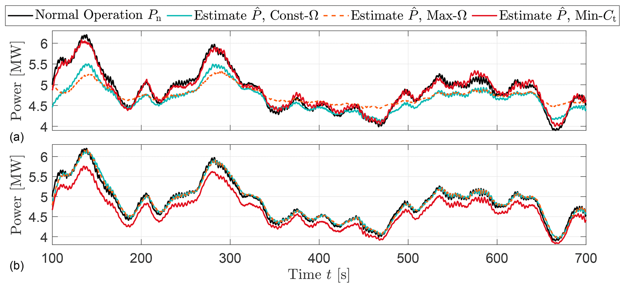
Figure 2Time series of normal power Pn and available power estimation based upon various down-regulation strategies. (a) and (b) indicate the estimation based on measurements of turbines operating at 40 % and 80 % of the rated power, respectively.
It should be noted that the sensitivity observed in the synthetic time series in Fig. 2 is expected to grow under the field conditions. This is due to the fact that the manufacturer-calibrated power coefficients cannot account for variability influenced by local conditions (Bandi and Apt, 2016). Additionally, the resulting uncertainty of the CP-dependent approaches is likely to also be amplified due to the lack of detailed information regarding the pre-defined CP and implemented operation strategy for curtailment caused by the limited access to the controller in practice. To avoid the dependency on operating point estimations of available power, the use of wind speed measurements is revisited with the state-of-the-art deep-learning architecture in the next section. The performance of this model-free approach is then compared with the presented wind speed observer, also for the scenario with limited CP information during down-regulation.
For a more robust operation and delta control, the bias and the uncertainties, which partly originate from the natural variability of the flow and turbulence and partly due to the uncertainty associated with the turbine models, i.e. CP surfaces, should be reduced. The former is investigated through a state-space update via Kalman filters in Sect. 2. Here, we implement a fully data-driven approach, which is purely based on the atmospheric inputs to eliminate the dependency of the estimated available power production to the CP surfaces and/or the control strategy.
Although the deep-learning techniques have been applied to numerous engineering fields, their application in wind farm flow modelling has been rather limited. For the turbine level power estimation, recently neural networks have been implemented to approximate the power curve mainly based on field data (for a detailed review, see e.g. Lydia et al., 2014). Pelletier et al. (2016) applied feed-forward neural networks (FFNNs) in a steady-state manner with six atmospheric inputs including shear and yaw error of the investigated turbine. Ouyang et al. (2017) approached the problem by sectioning the regions of the power curve and developed a support vector machine algorithm for each partition, capable of capturing the dynamic response of the turbine. Manobel et al. (2018) on the other hand underline the importance of data filtering and normal behaviour recognition for such problems and also indicate that the architecture of the neural network needs to be re-optimized for each turbine within a wind farm, to increase accuracy.
Here in this study, we use the open-source machine learning repository, TensorFlow (Abadi et al., 2016) to implement the LSTM algorithm. LSTM architecture is a special type of RNN, which is shown to perform faster and better for highly fluctuating time series than many other RNN architectures. An LSTM neuron is illustrated in Fig. 3, where there is no direct connection between the input it and the output ot gates. All the information flows through the cell state ct, which is the actual memory of the LSTM neuron, and it is regulated by the forget gate ft to avoid indefinite growth and eventual network break down (Gers et al., 2000). Through the calibrated weights, ft decides how much of the previous cell state(s) is preserved, following Eq. (4).
where σ represents the sigmoid gate, xt is the input tensor of the current state and ht−1 is the output tensor of the previous state of the cell. Wfi and Wfo are the weights applied to input and output tensors of the forget gate, and bf is the bias vector. Information is then transferred to the input gate it which is then forwarded to the cell state, ct, where it is selectively saved in the long-term memory. The mathematical procedure can be written as Eqs. (5) and (6).
with Wii and Wio as the weights applied to input and output tensors of the input gate respectively and bi as the bias vector. The previous cell state, ct−1, is then updated via
The updated cell state ct then feeds regulated information to the output gate and finally the actual output of the neuron via Eqs. (7) and (8).
Similarly Woi and Woo are the weights applied to input and output tensors of the output gate respectively, and bo is the corresponding bias vector. The final output of the cell is then defined using ot and ct via the tanh function by
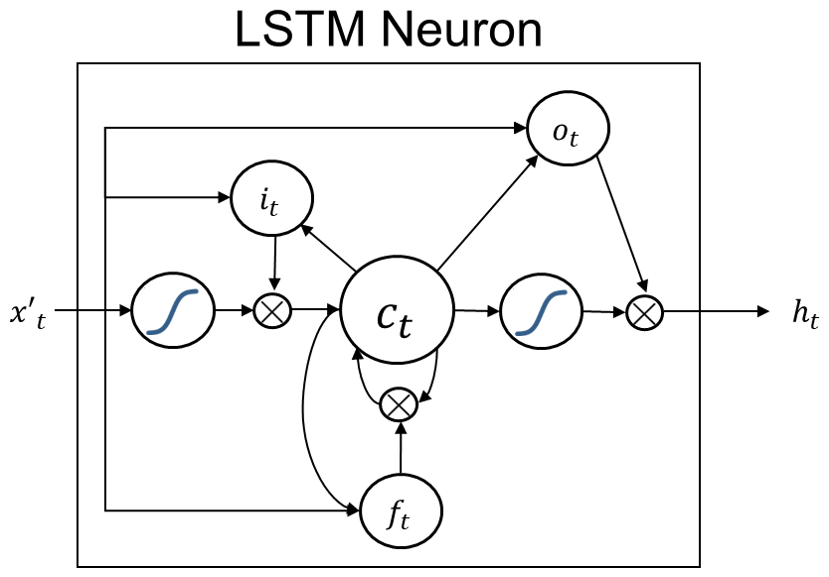
Figure 3LSTM neuron with cell state ct, as well as input it, output ot and forget ft gates. and ht indicate the inputs and outputs of the neuron, respectively. The curves represent sigmoid gates, σ.
LSTM algorithms are heavily used in a variety of sequential and temporal predictive modelling, from language processing (e.g. Gers and Schmidhuber, 2001) to short-term forecasting (e.g. Zhang et al., 2019). However, they require large amounts of data and computational resources to reach their full potential and achieve a generic solution without over-fitting. Therefore, although RNNs (and LSTMs in particular) have additional capabilities of modelling longer-term temporal properties, they remain highly challenging to train, especially with limited training data. In recent years, the transfer learning (or knowledge transfer) approach that addresses such problems (Pan and Yang, 2010) has been increasingly popular. The basic idea of the transfer learning is that a well-trained model and its hyper-parameters that involve rich knowledge of the target task can be used to guide the training of other models.
Throughout the rest of this section, we will firstly present the details of the architecture and the hyper-parameter tuning of an LSTM model fully trained on 3 h of HAWC2 simulations and compare the initial performance of LSTM neurons with simpler perceptrons in FFNN. We will then challenge our LSTM network to perform on another case with a different inflow condition than the original training domain. In pursuit of better performance on a different flow case, we will present the results from blind training as well as the transfer learning. We will then discuss their behaviour in terms of both the resulting error distributions and fitted parameters in between the layers. Finally, we will extend the application of the transfer learning to other flow cases, to demonstrate the flexibility and automation of the approach.
3.1 Data pre-processing and training strategy
The investigated case studies for available power estimation are generated and implemented using HAWC2 simulations with the DTU 10 MW reference wind turbine. For the training of the LSTM models, the high-frequency (100 Hz) wind speed signals from HAWC2 are down-sampled to 1 Hz, which is equivalent to the supervisory control and data acquisition (SCADA) system of a wind turbine (Göçmen and Giebel, 2018). The second input to the model is a moving (or rolling) standard deviation of the 1 Hz wind speed, with a 10 min rolling window as an indication of inflow turbulence intensity (TI). In contrast to the regular definition, this approximation of TI assures the same number of samples for both of the inputs.
The two inputs of wind speed and its moving standard deviation are first normalized between (0, 1) and then fed to the LSTM network to predict the power output during normal operation. As an LSTM neuron expects a three-dimensional input shape on the order of samples, lag and features, the input data are shaped accordingly. For the defined architecture with two input features listed above, the hindsight horizon to base the real-time estimations on is another hyper-parameter to be tuned. The hindsight horizon, or lag, is the number of previous time steps that have been taken into account to predict the power output in the current time step. Note that longer lag would increase the initialization period for the curtailment implementation and could be a limiting factor if the architecture is to be further adapted for online learning/training. Accordingly, for the LSTM networks the lags of 4, 9, 29, 59 and 89 s are investigated. Note that since the model is trained to map the atmospheric inputs to the actual production data under normal operation, the power predictions are ensured to follow the normal operation trend that is required for the available power estimation and not affected by the curtailment strategy.
For the preliminary evaluation of the training and hyper-parameter tuning of the model, a split validation dataset is generated. The final test of the model is based on an independent time series with a similar mean wind speed and turbulence intensity but covers a shorter time period. Since the target application of the model is to estimate real-time available power for more certain delta control (or reserve provision), the main criteria of evaluation is the 1 Hz error distribution for shorter test cases (10 min), where grid code compliance is tested for longer available periods (1 h) based on 1 min error distributions.
3.1.1 Training of the first LSTM model: low wind speed, high turbulence intensity
The case study to train the first LSTM model consists of a 3 h period, where hub-height wind speed and corresponding moving TI are used to estimate the power output of DTU 10 MW turbine under nominal operation. The input time series are presented in Fig. 4.

Figure 4First LSTM model training input time series generated by HAWC2, down-sampled to 1 Hz. Mean wind speed = 7 m s−1; mean TI = 10 %.

Figure 5Training history of the first LSTM network with mean wind speed = 7 m s−1, mean TI = 10 % and time lag = 29 s. The network architecture is presented in Table 2, where batch size = 60 with Adam optimization algorithm and mean absolute error (MAE) loss function implemented. The training is stopped at epoch = 100, after which the network training starts to show symptoms of overfit.
In order to have an adequate quantity of training samples while assuring a representative test dataset for hyper-parameter tuning, the 3 h period of training and validation signals is split as 80 % and 20 %, respectively. Since the target available power output is 1 Hz, the final model needs to be able to handle high-frequency dynamics in the inflow and successfully map it to the produced power in normal operation, by taking the inertia into account. Given the complexity the model is required to manage, the minimum number of neurons per layer is kept at 50 where two to three hidden layers are evaluated as candidate architectures. Table 1 compares the performance of different network configurations on validation data, for both more traditional FFNN perceptrons and LSTM neurons with lag = 29 s. It shows overall higher performance for LSTM configurations, indicating added value of using neurons with memory capabilities. In fact, LSTM is shown to also outperform more modern architectures such as extreme learning machine (ELM) (Saini et al., 2020) and Gaussian mixture models (GMMs) (Zhang et al., 2019) for short-term forecasting. Given the best overall performance, the final network has three hidden layers with 100, 100 and 50 LSTM neurons, as detailed in Table 2. The hyperbolic tangent function, tanh, is used as the activation function in between the layers. With the listed input structure, the final architecture corresponds to approximately 7 times more data than the trainable parameters, slightly less than the general rule of thumb to avoid overfitting; hence even higher numbers of neurons are avoided. Nevertheless, the training history in Fig. 5 and the model performance on the validation dataset do not indicate a clear overfit, increasing confidence in the training. For the mean absolute error as the loss function, the training history on the very first epoch for validation data shows “too good” performance of the initial fit. However, since it clearly does not indicate an overall higher accuracy, the network is trained further to its fuller potential, where the validation loss is expectedly lower and convergence is achieved around 100 epochs.
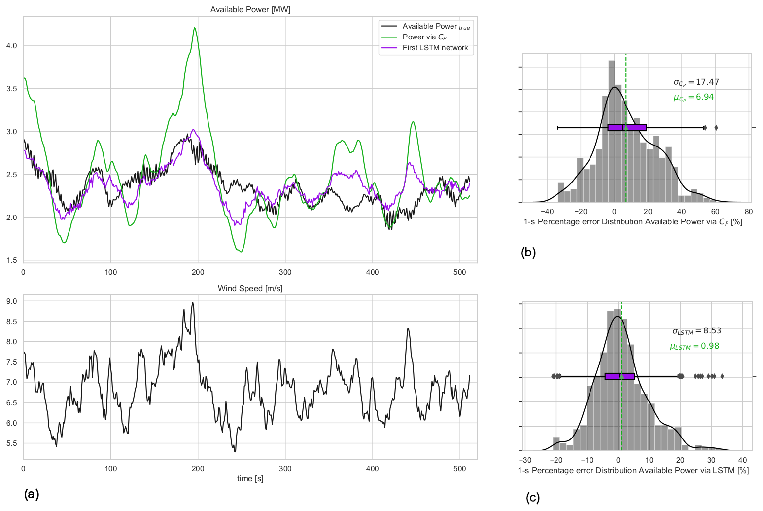
Figure 6(a) The 1 Hz time series of available power and wind speed for the first test case: second-wise comparison of the available power of the 10 MW turbine for mean wind speed = 7 m s−1 and mean TI = 10 % flow case represented in Fig. 4. (b) Available power estimation error via direct CP curve interpolation of wind speed; (c) error distribution of the first LSTM model with lag = 29 s. μ and σ are the mean and the standard deviation of the 1 Hz percentage error distributions.
Table 1Representative grid search for best architecture of the first network using feed-forward neural networks (FFNNs) and LSTM with lag = 29 s and tanh activation function in between the hidden layers. Both FFNN and LSTM trained using the Adam optimization algorithm and mean absolute error loss function. The listed percentage error estimation with mean μerr and standard deviation σerr is based on the validation dataset where .
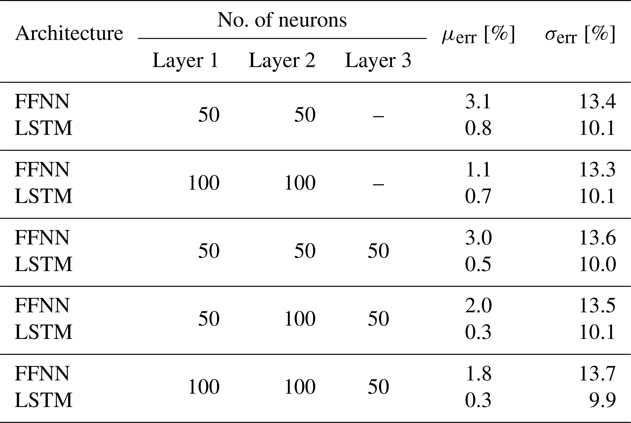
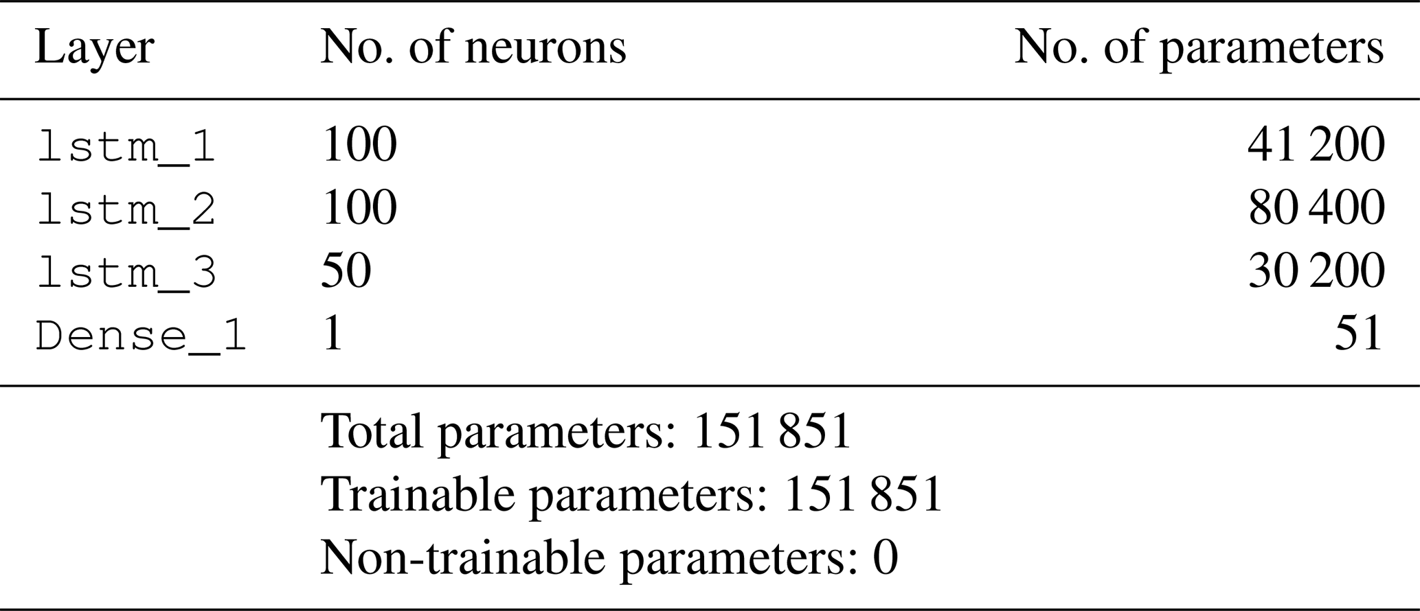
Table 2Architecture of the first LSTM network with lag = 29 s. Hidden layers: lstm_1, lstm_2, lstm_3. Output layer: Dense_1. tanh is used as the activation function in between the hidden layers.
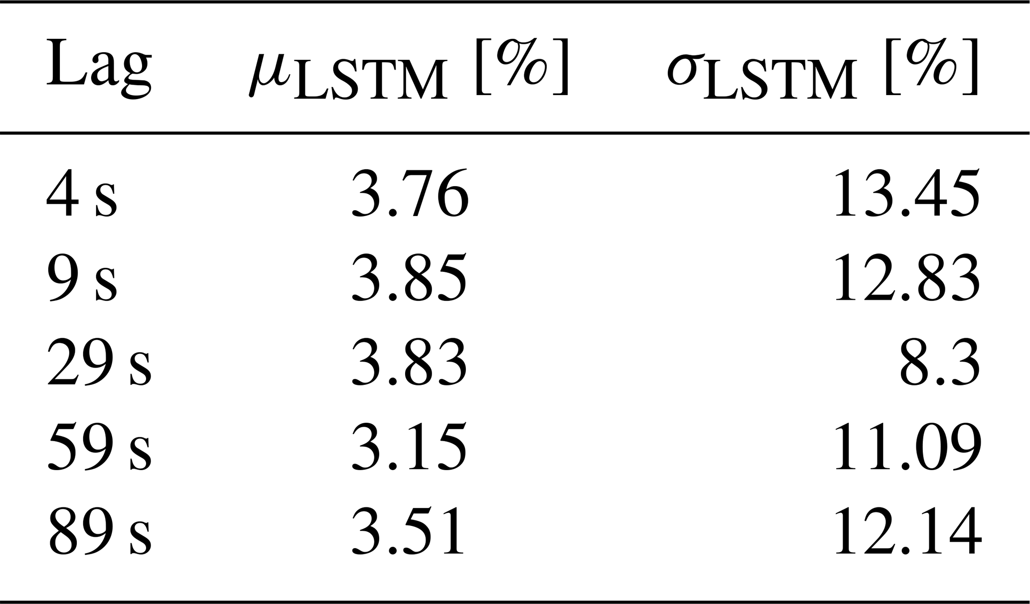
The first LSTM network is tested on a separate 10 min dataset and compared with the true available power (actual production of the DTU 10 MW turbine under normal operation) as well as the predecessor method of pre-defined CP look-up tables of the same turbine. The 1 Hz time series and the corresponding 1 s percentage error distribution of the direct CP look-up table approach and the LSTM model results with lag = 29 s are presented in Fig. 6. The sensitivity of the mean, μLSTM, and the standard deviation, σLSTM, to the hindsight horizon up to 89 s is listed in Table 3. Due to highest overall performance, the results from the LSTM model with lag = 29 s will be discussed from now on.
Table 3Sensitivity of the first LSTM model to the hindsight horizon, evaluated based on test dataset.
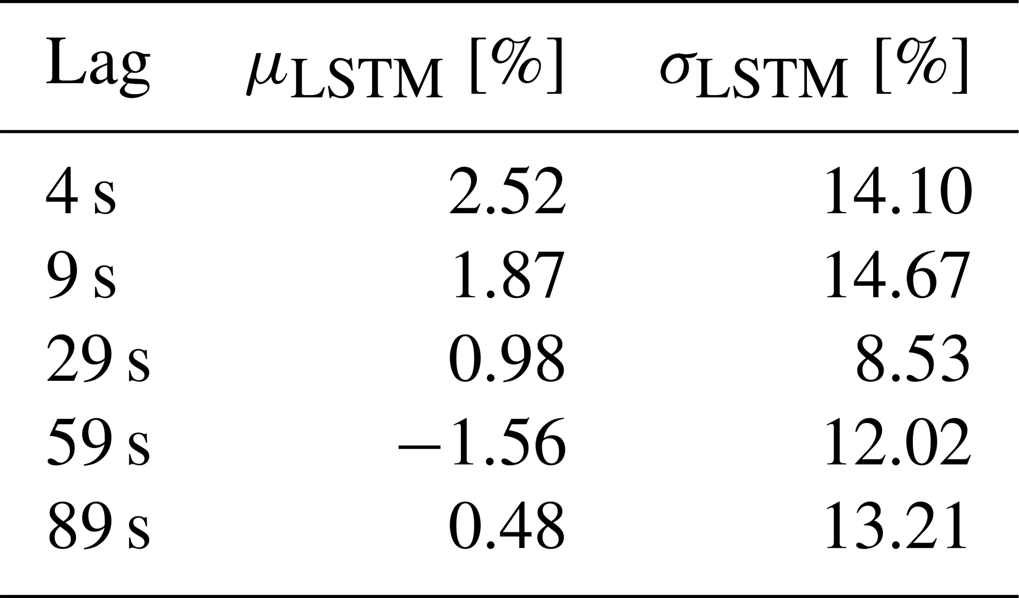
Figure 6 shows that the LSTM model significantly improves the agreement between the actual and the predicted available power production compared to the direct CP curve interpolation. Since both the trained LSTM model and the CP curve interpolation approach use the same input (hub-height wind speed), it can be said that the described deep-learning architecture is much more capable of reproducing the dynamic power curve of the turbine than the steady-state CP surface, even with limited information. For the investigated 10 min period, the bias in the second-wise LSTM available power predictions is less than 1 %, as opposed to nearly 7 % observed with the direct CP interpolation approach, where the percentage error is defined as with y(ti) being the power produced by DTU 10 MW under normal operation, i.e. available power, and is the LSTM model prediction at every time step ti. The standard deviation of the second-wise error distribution, which is regarded as an indication of uncertainty in the model results for this study, is also reduced significantly to 8.5 %. Note that it is expected to further decrease when the available power prediction is to be delivered at larger timescales (e.g. highest frequency being the 1 min scale as requested by the German TSOs; 50Hertz, Amprion, Tennet, TransnetBW, 2016). This will be discussed further for larger evaluation periods later in the study.
3.1.2 Training of the second LSTM model: high wind speed, high turbulence intensity
One of the most crucial challenges of purely data-driven models is the fact that they are not valid for the input variables outside the training domain, also referred to as the generalization problem. As seen in Fig. 4 the first LSTM model is trained for a mean wind speed of 7 m s−1, where the turbulent fluctuations occasionally reach above 8 m s−1. However, for higher wind speeds, e.g. around 9 m s−1, the first LSTM model is expected to perform poorly as it has not been taught to map the relationship between wind speed, TI and power for that inflow.
In order to reduce the effort in hyper-parameter tuning and test the universality of the network architecture for a similar problem, the same configuration as in Table 2 is implemented with the inflow time series presented in Fig. 7. The final model is referred to as the second LSTM model throughout this study.
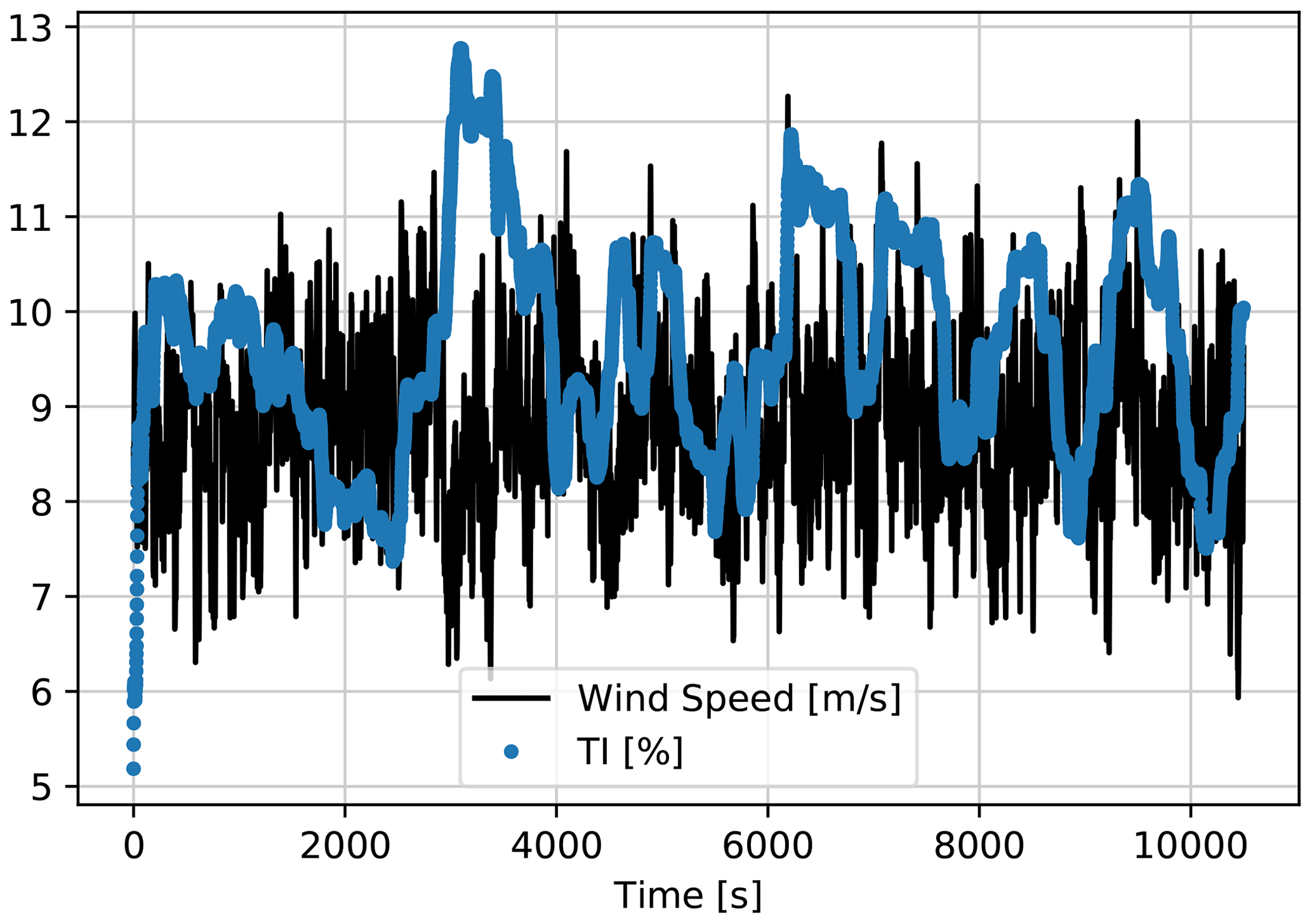
Figure 7Second LSTM model training input time series generated by HAWC2, down-sampled to 1 Hz. Mean wind speed = 9 m s−1; mean TI = 10 %.
The performance of the second model is evaluated based on an independent 10 min series with similar mean wind speed and TI and compared with the direct CP interpolation approach. Similar to the first LSTM model, the test results are presented for lag = 29 s in Fig. 8.

Figure 8(a) The 1 Hz time series of available power and wind speed for the second test case: second-wise comparison of the available power of the 10 MW turbine for mean wind speed = 9 m s−1 and mean TI = 10 % flow case represented in Fig. 7. (b) Available power estimation error via direct CP curve interpolation of wind speed; (c) error distribution of the second LSTM model with lag = 29 s. μ and σ are the mean and the standard deviation of the 1 Hz percentage error distributions.
Despite the significant performance improvement achieved for the 7 m s−1 case with the first LSTM observed in Fig. 6, the second LSTM network developed using the same procedure for 9 m s−1 inflow has a considerable bias of more than 3 % as seen in the 1 Hz percentage error distribution in Fig. 8. The mean of the test error seems to be hardly affected by the changing hindsight horizon listed in Table 4, where the standard deviation is the least at lag = 29 s. This clearly implies that the architecture and the hyper-parameters optimized for the lower wind speed are not necessarily the best configuration for slightly higher wind speed cases. That trend makes it challenging to develop a generic network architecture that would successfully reproduce the high-frequency available power for all the possible input realizations. It indicates the need to specifically tune the hyper-parameters for each separate flow case. It is a cumbersome process with high computational cost. Here in this study, the focus is to make the best out of the available dataset, as indicated earlier, as the generation (or collection) of a comprehensive database is a very demanding task for high-frequency problems. Additionally, the observed reduction in performance of the same hyper-parameter space for a different flow case indicates the risk of the approach where a singular “generic” model is fit to estimate the high-frequency available power for a variety of inflow cases. In other words, a single model to cover the entire domain might introduce compromises in the model performance at certain inflow cases, where the dynamic accuracy is of the utmost importance, as framed by the grid codes.
Table 4Sensitivity of the second LSTM model to the hindsight horizon.
3.1.3 Transfer learning from the first model: high wind speed, high turbulence intensity
Having trained a well-performing model for the first inflow case with 7 m s−1 mean wind speed and 10 % mean TI, the following question arises: can some of the characteristics of the first model be conveyed to a different flow case to achieve similarly good results? Transfer learning can provide a valuable platform for such model extensions, as it is used to improve a learner from one domain by transferring information from a related domain (Weiss et al., 2016). This enables a systematic model update when new data are available from outside the training domain. Accordingly, part of the first model with 7 m s−1 mean wind speed would be transferred to update some of the parameters for higher wind speed. The procedure could be repeated for all the changing wind speed and TI cases, in both HAWC2 platform and field applications.
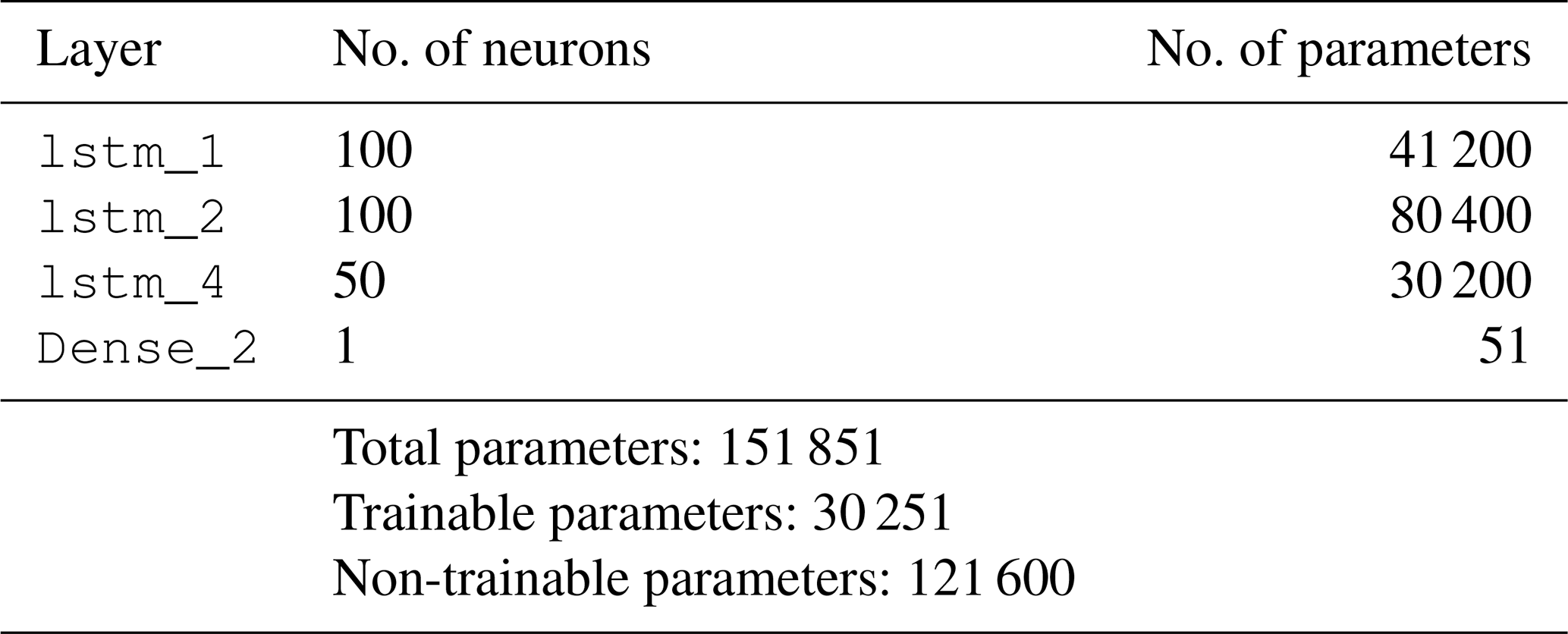
To assess the transferability of the parameters, the trends of the weights trained for the first (Network_1) and the Second (Network_2) LSTM networks are compared in Fig. 9. The actual probability seen in the most recent histograms (the lightest shade in the series of distributions) are different for all three LSTM layers, with larger tails on Network_1 distributions. However, the range of values for the output weights of the first layer lstm_1 and the second layer lstm_2 are very similar, with an interquartile range of for both. On the other hand, the third and shallower layer lstm_3 seems to optimize for significantly different weights for different inflow velocities. Therefore, it is concluded that the first two LSTM layers are transferable from the first LSTM network, where the last LSTM layer as well as the output layer need to be re-tuned for changing inflow case(s). The resulting architecture is presented in Table 5 where the number of trainable parameters is significantly reduced. Accordingly, the transferred architecture is a much lighter network that ensures fast training, while enclosing a profound amount of information from previous learning(s). Fewer parameters also enables a robust training with shorter time series. Hence, for the training of the transfer learning LSTM architecture, 60 % of the dataset (second inflow case, presented in Fig. 7) is fed to the network, where 40 % is left for validation to ensure a more definitive assessment of the training.
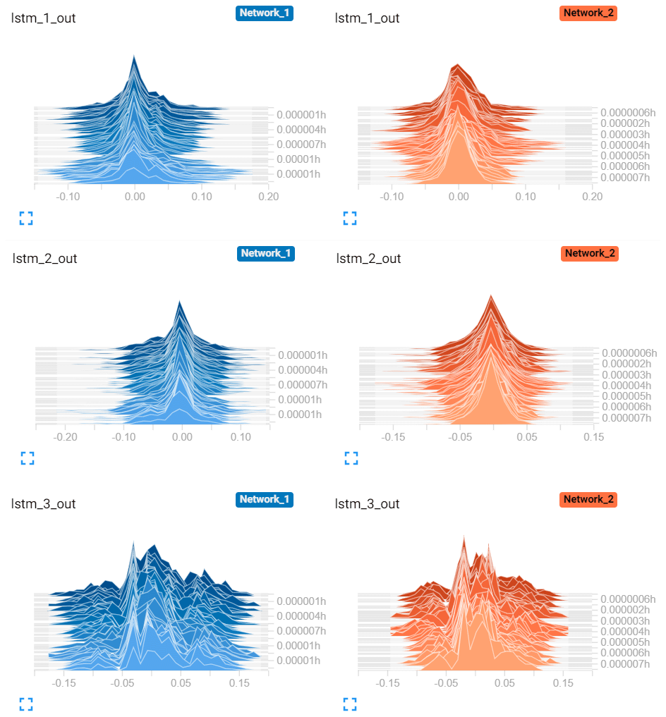
Figure 9Distribution of the output tensors of each hidden LSTM layer for the first Network_1 and the second Network_2 LSTM networks, visualized via TensorBoard. Each slice displays a single histogram updated at each iteration. The “oldest” iterations are further back and darker, while the “newer” ones are lighter and closer to the front. The y axis indicates the relative time of each update.
Table 5Architecture of the transferred LSTM network for lag = 29 s. Hidden layers: LSTM_1, LSTM_2, LSTM_4. Output layer: Dense_2. Frozen layers: LSTM_1, LSTM_2 (same layers as in the first LSTM model in Table 2). Trainable layers: LSTM_4, Dense_2. tanh is used as the activation function in both of the activation layers. Training is performed with batch size = 60, the Adam optimization algorithm and a mean absolute error loss function over epoch = 70.
Apart from an update of the weights in the last LSTM and the output layers (lstm_4 and Dense_2 in Table 5, respectively), none of the other hyper-parameters were changed in the training process of the transferred LSTM network. This provides a certain repeatability to the training process, where the last two layers can be updated when a new flow case is encountered by the turbine. It is particularly an important feature for the control implementation as it enables fast online learning and continuous improvement of the model.
To put the performance of the transferred LSTM model to the test, the same test case as in the second LSTM model in Fig. 8 is considered. This time, the estimations from the operation-dependent wind speed observer (WSO) approach (described in Sect. 2) are also compared with the transferred LSTM model. The time series in Fig. 10a illustrates the sensitivity of the WSO estimations to the operation strategy under 40 % down-regulation with constant rotational speed, Const-Ω, and maximum rotational speed, Max-Ω, and following the minimum thrust coefficient, Min-Ct. In Fig. 11a–c, the error distributions of the WSO estimations under those three operational strategies are presented. While the overall performance of all WSO estimations is highly compelling, the results also indicate up to 4 % variation in the mean bias of the WSO model. With the minimum mean error of 0.26 %, WSO estimations with maximum rotational speed, Max-Ω, are also compared with the transferred LSTM model in Fig. 10c. For the investigated setup with the DTU 10 MW reference turbine model fully recognized, the WSO results generally suggest a better agreement with the true available power, quantified in Fig. 11d. However, Figs. 10c and 12 point out that for a potential mismatch of 5 % in the pre-defined and operational CP surfaces due to several uncertainties listed earlier, model-based WSO results show bias of up to more than 6 % where the model-free LSTM performance remains unaffected. Note that in these WSO runs, we assume “perfect knowledge” for normal operation, i.e. for maximum CP, and 5 % uncertainty for the rest of the CP domain. This simulates the field operation where the nominal power curve is corrected for the site conditions (hence perfect knowledge) but the information of the rest of the operational CP remains limited.
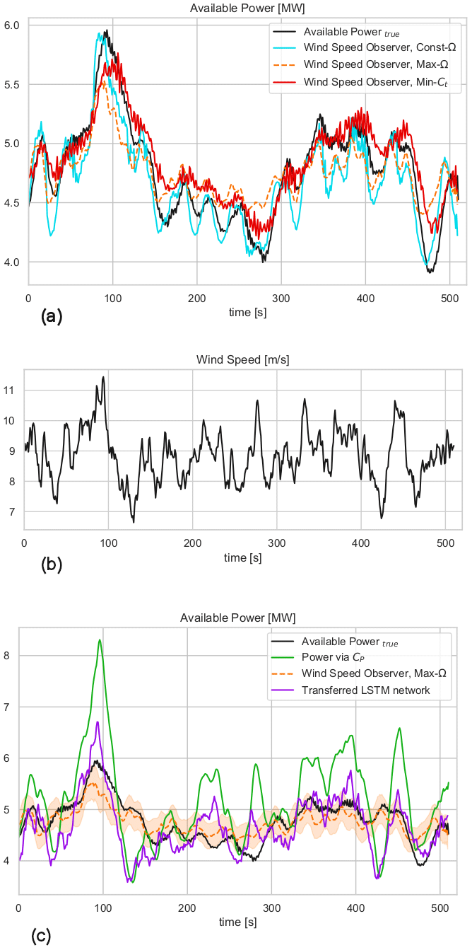
Figure 10The 1 Hz time series comparison of available power of DTU 10 MW turbine, estimated by (a) the wind speed observer for the 40 % down-regulation case under three different curtailment strategies; see Sect. 2. (b) Second-wise wind speed time series of the considered test case with mean wind speed = 9 m s−1 and mean TI = 10 %. (c) The comparison of the available power estimated via wind speed observer following the maximum rotational speed control strategy and LSTM network with transfer learning from the lower wind speed to higher wind speed cases and direct CP approach. The shaded area corresponds to the effects of ±5 % over- and underestimation of CP during curtailment for WSO results. The LSTM network has no dependency on level of curtailment or estimation of operational CP.
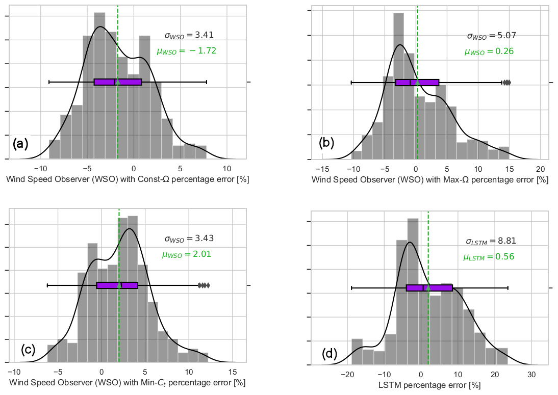
Figure 11The 1 Hz percentage error distribution of the available power estimation of the 10 MW turbine for mean wind speed = 9 m s−1 and mean TI = 10 %, the flow case represented in Fig. 7. The presented performances belong to the wind speed observer approach, presented in Sect. 2, under different operational strategies. (a) Constant rotational speed, Const.-Ω; (b) maximum rotational speed, Max-Ω; (c) minimum thrust coefficient, Min-Ct, as 40 % curtailment strategy; (d) LSTM model with transfer learning from lower wind speed to the higher wind speed case (no dependency on the curtailment strategy).
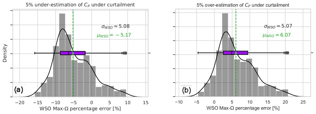
Figure 12(a) Sensitivity of wind speed observer to correct assessment of CP under curtailment. The simulations assume “perfect knowledge” of CP for the normal operation and 5 % uniform uncertainty for the rest of the operational range. (a) The 1 Hz percentage error of WSO with Max-Ω: 5 % under-estimation of CP during curtailment. (b) The 1 Hz percentage error of WSO with Max-Ω: 5 % over-estimation of CP during curtailment.
It is also seen that the transferred LSTM model outperforms the second LSTM model where more than 3 % model bias is eliminated compared to Fig. 8d. This improvement is very promising for the implementation of the transfer learning for modelling high-frequency time series with LSTM networks. Furthermore, the results also show the potential of such a deep-learning approach for avoiding the operational dependencies of dynamic delta control with relatively low uncertainties. The adaptation capabilities of transfer learning are to be tested with additional flow cases in the next sections.
3.1.4 Further transfer learning to higher wind speed flows
With the comparable results of the model-free transfer learning LSTM networks to the model-dependent WSO approach, even with potentially lower uncertainties in the simulation environment compared to the field implementation, here we test the approach for even higher wind speed flows. The first LSTM predictions were built and tested on 7 m s−1 mean wind speed, where its information from the first two layers is then transferred to estimate the available power for the 9 m s−1 mean wind speed case. Here we further update the LSTM network to extend the training (and validity) domain to the 11 m s−1 mean wind speed range, using the generated time series in Fig. 13. Note that for all three steps of the learning, the mean TI remains 10 % to isolate the effect of wind speed on the network performance.
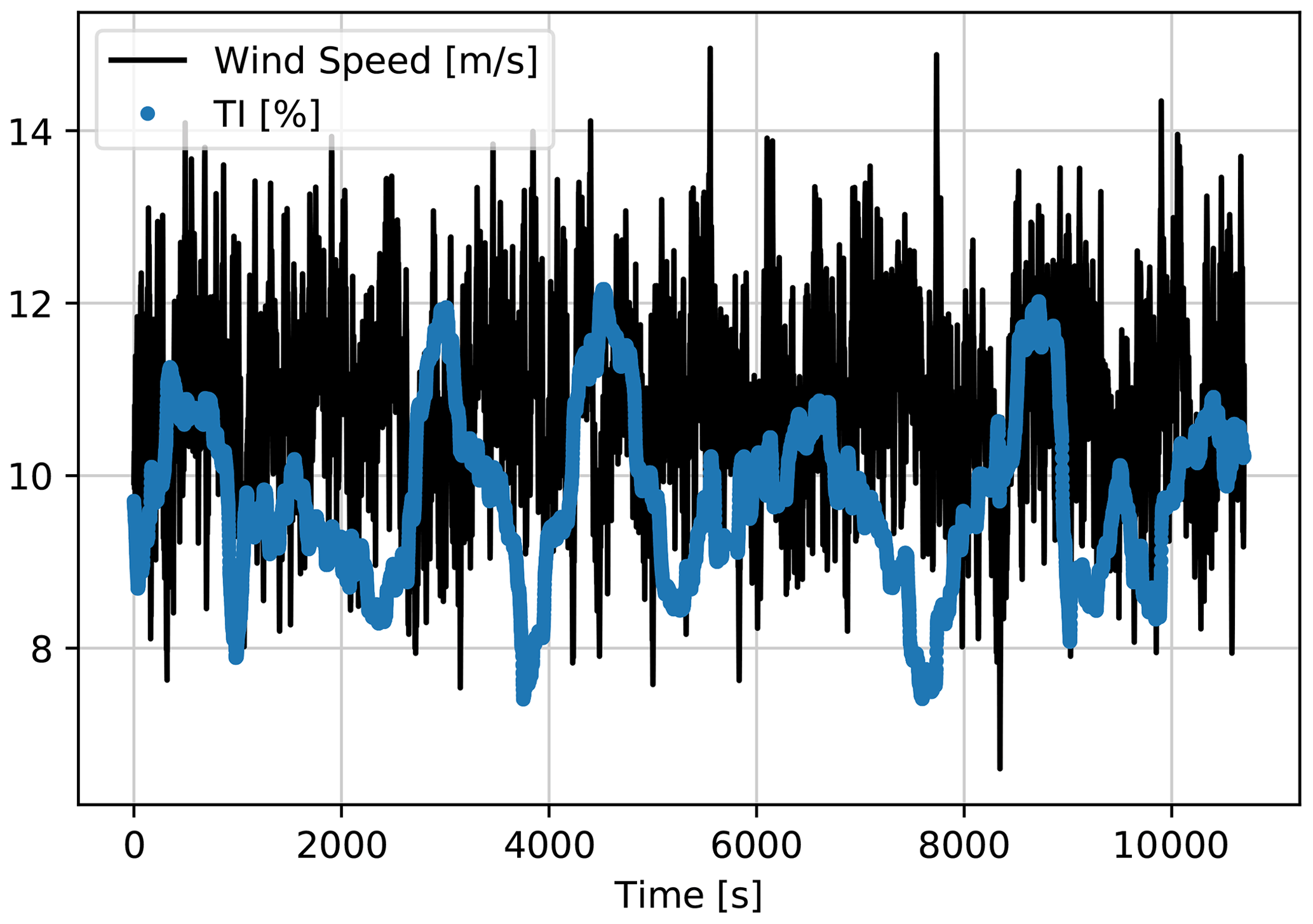
Figure 13LSTM network training with further transfer learning input time series generated by HAWC2, down-sampled to 1 Hz. Mean wind speed = 11 m s−1; mean TI = 10 %.
The resulting network with further transfer learning for 11 m s−1 mean wind speed (in Fig. 14a) performs similar to in the 9 m s−1 (in Fig. 11d) and 7 m s−1 (in Fig. 6d) mean wind speed cases with less than 1 % second-wise percentage error on average. Distinctly from the previous inflow cases, the tail towards the positive percentage error is longer in the final 1 Hz error distribution in Fig. 14a. This is mainly due to the fact that the DTU 10 MW reference turbine (with rated wind speed 11.4 m s−1) occasionally enters the rated region according to the turbulent fluctuations around 11 m s−1 mean wind speed. Nevertheless, the variability of the model prediction error is significantly reduced when averaged for a 1 min scale in Fig. 14b. The results show that the model-free transfer learning approach easily complies with the strictest TSO requirements in provision of the available power signal; i.e. the standard deviation of the 1 min percentage error of the available power is required to be less than ±3.3 % as stated in 50Hertz, Amprion, Tennet, TransnetBW (2016).
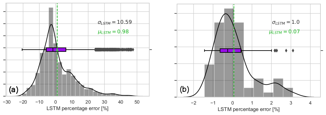
Figure 14LSTM network prediction error for the further transfer learning flow case. Mean wind speed = 11 m s−1 and TI = 10 % over the 60 min validation case. (a) The 1 Hz prediction error; (b) the 1 min average prediction error.
3.1.5 Network performance on higher turbulence intensity
As stated earlier, for all three inflow cases where the first LSTM network is generated and extended via transfer learning, the mean turbulence intensity remained TI = 10 %. Here in this section, the models are tested under higher turbulence intensity (TI = 20 %) with the same corresponding mean wind speed. Note that the generated network structures, i.e. the first LSTM model (7 m s−1 mean inflow speed), transfer learning LSTM model (9 m s−1 mean inflow speed) and further transfer learning LSTM model (11 m s−1 mean inflow speed), are not updated for higher-TI cases. In other words, here we aim to test the capability of the trained networks under higher TI with the same mean wind speed for the inflow, without further model update.
Figures 15–17 focus on highly turbulent inflow cases (TI = 20 %) and show the corresponding performance of the three neural networks trained and updated for increasing wind speeds via transfer learning. It is seen that the 1 min average prediction errors of the models are consistently low for highly turbulent flows as well; hence further training (or model update) is not required. The maximum standard deviation of 1 min averaged percentage error is still less than 3.3 % with the largest bias of 1.3 %, which is slightly worse than the test results in the original domain of the networks. For the mean wind speeds of 7 and 9 m s−1, the effect of higher turbulence levels is clearer as increasing fluctuations in wind speed are directly correlated to higher variance in power output. However for the 11 m s−1 case, the fluctuations are partially dampened due to the turbine entering into the rated region. Overall, it can be said that the sensitivity of the networks to changing wind speed is much higher than the turbulence, and the updates are to be implemented solely based on the altering inflow velocity, which is likely to reflect a different operational region. The available power prediction of the described LSTM architecture and the updating scheme with 2 m s−1 wind speed increase (7–9–11 m s−1) is shown to comply with the strictest grid code requirements under different turbulence realizations.
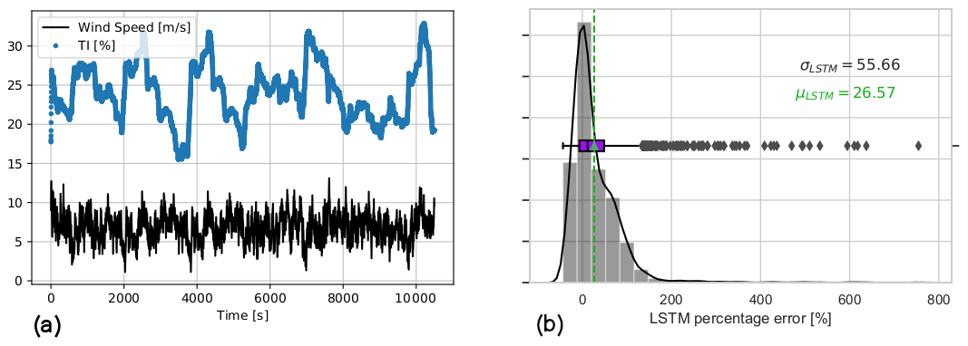
Figure 15Input time series and 1 min prediction error of the first LSTM network, higher-turbulence-intensity flow case. Mean wind speed = 7 m s−1 and TI = 20 % over the 60 min validation case. (a) Time series of the inflow dataset for the higher-TI test of the first LSTM network, originally trained on mean wind speed = 7 m s−1 and TI = 10 %. (b) The 1 min average percentage error of the first LSTM network tested under higher TI.
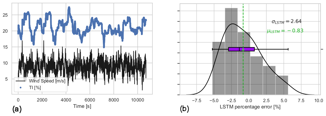
Figure 16Input time series and 1 min prediction error of the transfer learning LSTM network, higher-turbulence-intensity flow case. Mean wind speed = 9 m s−1 and TI = 20 % over the 60 min test case. (a) Time series of the inflow dataset for the higher-TI test of the transfer learning LSTM network, originally trained for mean wind speed = 9 m s−1 and TI = 10 %. (b) The 1 min average percentage error of the transfer learning LSTM model under higher TI.
Figure 17Input time series and 1 min prediction error of the further transfer learning LSTM model, higher-turbulence-intensity flow case. Mean wind speed = 11 m s−1 and TI = 20 % over the 60 min test case. (a) Time series of the inflow dataset for the higher-TI test of the further transfer learning LSTM model, originally trained for mean wind speed = 11 m s−1 and TI = 10 %. (b) The 1 min average percentage error of the further transfer learning LSTM model under higher TI.
The dynamic estimation of available power of a wind turbine is essential for both power system stability and marketability of the reserve power. The current estimations are highly sensitive to the down-regulation strategy and prone to turbine model uncertainties and inadequacies. Here we propose a purely data-driven, model-free methodology based on long short-term memory (LSTM) neural networks. This state-of-the-art deep-learning architecture is implemented to map the available power of the DTU 10MW reference turbine under turbulent inflow generated in HAWC2. The trained networks are adapted to the changes in incoming mean wind speed via transfer learning, where only the parameters in the last layer are updated when the new inflow information is available.
The first LSTM network has three hidden layers with 100, 100 and 50 neurons which is trained using 1 Hz power output under normal operation with 7 m s−1 mean wind speed and 10 % turbulence intensity (TI). A performed test on a separate 10 min flow case with the same mean wind speed and TI shows less than 1 % bias and less than 9 % standard deviation. The same architecture is used to train the second LSTM network with an increase in mean wind speed to 9 m s−1 and the same TI level of 10 %. Although the width of the distribution is similar, the bias has increased to almost 4 %, indicating the need to re-tune the hyperparameters of the architecture. In fact, the comparison of the fitted parameters between the first LSTM and the second LSTM networks for each layer shows analogous distributions of the weights. This further motivates the transferability of the learnings of the first two LSTM layers, where only the parameters of the last layer need to be updated for the changing incoming mean wind speed. With a significant reduction in the number of parameters to fit, the transferred LSTM network has the capability of faster and more robust training, even with limited data. The performance of the transferred LSTM network is also evaluated using a separate 10 min time series with 9 m s−1 mean wind speed and 10 % TI. The results are very comparable with the outcome of the first LSTM model, which demonstrates the adaptability of the network to changing inflow conditions with the update of the last LSTM layer. The transferred LSTM also outperforms the second LSTM network with a significant decrease in bias (around 0.5 %), eliminating the need to re-tune the hyperparameters or developing a new network structure from scratch.
The transferred LSTM network is also compared with the model- and operation-dependent wind speed observer (WSO) approach. For the investigated setup where the DTU 10 MW reference turbine model is fully transparent or known, the WSO results generally suggest a better agreement with narrower 1 Hz percentage error distributions. However, the sensitivity of the WSO approach to the curtailment strategy is also clearly seen as the results indicate up to 4 % variation in the mean bias of the WSO model. The uncertainty of the approach is expected to grow further under the field conditions where there is a potential lack of detailed information regarding the operation strategy and manufacturer-calibrated power coefficients which are generally unable to account for variability influenced by local conditions. To test that hypothesis, 5 % uniform uncertainty is introduced to the CP surface under curtailment for the same evaluation period. Even for the estimation based on the best-performing model under the maximum rotational speed control strategy, the model bias significantly increased, risking both under-estimation ( %) and over-estimation (bias>6 %) of the available power for the assigned CP uncertainty.
To ensure the applicability of the transfer learning to several inflow cases, the approach is tested for even higher wind speed flows. Further transferred LSTM network is trained only to update the last LSTM layer with 11 m s−1 mean wind speed and the 10 % TI case, where the first two layers come from the first LSTM model with 7 m s−1 mean wind speed validity domain for the same TI. The performance of the further transferred network is evaluated within the framework of strict grid requirements, where the quality of the available power signal is to be assessed at 1 min intervals with required accuracy of less than 3.3 % standard deviation of the error distribution. Corresponding 1 min average percentage error of the further transferred network indicates easy compliance with the regulations, with both bias and standard deviation less than 1 %. Similar agreement is observed when all the networks (i.e. first LSTM with 7 m s−1 wind speed, transferred LSTM with 9 m s−1 wind speed and further transferred LSTM with 11 m s−1 wind speed) are tested under higher TI of 20 %, indicating the robustness of the developed algorithm.
Finally, it should be noted that the neural networks with transfer learning ability used in this study can easily be implemented in operating wind turbines in the field. The second-wise wind speed input to the approach can be provided either from the standard nacelle anemometers or additional sensors such as meteorological masts or remote sensors (e.g. lidars, radars); however, associated input uncertainties should be handled carefully. This study is conceptual evidence that well-trained neural networks can be applied to determine the set point for implementing delta control, or to assess the level of reserves when using balance control, even with limited information in the field conditions. The transferability of the network adds the ability for online learning which ensures the continuous improvement of the model-free available power estimation.
The networks developed in this study can be extended to forecast applications, where the input that is read throughout the hindsight horizon (e.g. 29 s for the cases presented here) is used to predict the available power in the forecast horizon longer than 1 s (e.g. 1 min ahead). Similarly, the approach can be implemented for several turbines within the wind farm. For this configuration, the wind direction should be defined as an additional input to take the correlations of local wake effects and power into account. Finally, the neural network algorithm can be updated given the developments within the deep-learning research over time. The advancements in the sequential processing (e.g. convolutional LSTMs where the internal matrix multiplications are exchanged with convolution operations, gated recurrent units (GRUs) where the three-gated LSTMs are “simplified” with an update and a reset gate) can easily be utilized when beneficial, keeping the approach up to date.
Both the data and the script to train the networks (first LSTM and transfer learning LSTM networks) can be accessed at https://doi.org/10.5281/zenodo.3531414 (Göçmen et al., 2020).
The LSTM network training as well as the transfer learning implementation is performed by TG. The need for such an approach is underlined by AMU, who also generated the time series in the DTU 10 MW turbine model in HAWC2. JL also contributed in defining the research gaps in the field and developed the implementation cases for the LSTM network as the set point for curtailment in the HAWC2 controller, therefore also ensuring the generalizability and validity of the code. AWHL contributed with the Kalman-filter-based wind speed estimator and the sensitivities of the current methods for available power estimation at the single-turbine level.
The authors declare that they have no conflict of interest.
This research has been supported by the Energistyrelsen (grant nos. 2016-1-12396 and 64017-0045) and the European Commission (grant TotalControl no. 727680).
This paper was edited by Gerard J. W. van Bussel and reviewed by Fausto Pedro García Márquez and Martin Felder.
Abadi, M., Barham, P., Chen, J., Chen, Z., Davis, A., Dean, J., Devin, M., Ghemawat, S., Irving, G., Isard, M., Kudlur, M., Levenberg, J., Monga, R., Moore, S., Murray, D. G., Steiner, B., Tucker, P., Vasudevan, V., Warden, P., Wicke, M., Yu, Y., Zheng, X., and Brain, G.: TensorFlow: A System for Large-Scale Machine Learning TensorFlow: A system for large-scale machine learning, in: 12th USENIX Symposium on Operating Systems Design and Implementation (OSDI '16), 2–4 November 2016, Savannah, GA, USA, ISBN 9781931971331, 265–284, https://doi.org/10.1038/nn.3331, 2016. a
Annoni, J., Taylor, T., Bay, C., Johnson, K., Pao, L., Fleming, P., and Dykes, K.: Sparse-Sensor Placement for Wind Farm Control, J. Phys.: Conf. Ser., 1037, 032019, https://doi.org/10.1088/1742-6596/1037/3/032019, 2018. a
Attya, A., Dominguez-Garcia, J., and Anaya-Lara, O.: A review on frequency support provision by wind power plants: Current and future challenges, Renew. Sustain. Energ. Rev., 81, 2071–2087, https://doi.org/10.1016/j.rser.2017.06.016, 2018. a
Bak, C., Bitsche, R., Yde, A., Kim, T., Hansen, M. H., Zahle, F., Gaunaa, M., Blasques, J., Døssing, M., Heinen, J. J. W., and Behrens, T.: Light rotor: The 10-MW Reference Wind Turbine, in: European Wind Energy Conference and Exhibition 2012, EWEC 2012, 16–19 April 2012, Copenhagen, Denmark, 2012. a, b
Bak, C., Zahle, F., Bitsche, R., Kim, T., Yde, A., Henriksen, L. C., Hansen, M. H., Blasques, J. P. A. A., Gaunaa, M., and Natarajan, A.: The DTU 10-MW Reference Wind Turbine, in: Danish Wind Power Research 2013, 27–28 May 2013, Denmark, https://doi.org/10.1017/CBO9781107415324.004, 2013. a
Bali, V., Kumar, A., and Gangwar, S.: Deep learning based wind speed forecasting- A review, in: Proceedings of the 9th International Conference On Cloud Computing, Data Science and Engineering, Confluence 2019, 26–28 February 2019, Orlando, FL, USA, https://doi.org/10.1109/CONFLUENCE.2019.8776923, 2019. a
Bandi, M. and Apt, J.: Variability of the Wind Turbine Power Curve, Appl. Sci., 6, 262, https://doi.org/10.3390/app6090262, 2016. a
Bhowmik, S., Spee, R., and Enslin, J. H.: Performance optimization for doubly-fed wind power generation systems, in: vol. 3, Conference Record of 1998 IEEE Industry Applications Conference, Thirty-Third IAS Annual Meeting (Cat. No. 98CH36242), 12–15 October 1998, St. Louis, MO, USA, 2387–2394, 1998. a
Chen, J., Zeng, G. Q., Zhou, W., Du, W., and Lu, K. D.: Wind speed forecasting using nonlinear-learning ensemble of deep learning time series prediction and extremal optimization, Energ. Convers. Manage., 165, 681–695, https://doi.org/10.1016/j.enconman.2018.03.098, 2018. a
Chinmoy, L., Iniyan, S., and Goic, R.: Modeling wind power investments, policies and social benefits for deregulated electricity market – A review, Appl. Energy, 242, 364–377, https://doi.org/10.1016/j.apenergy.2019.03.088, 2019. a
50Hertz, Amprion, Tennet, TransnetBW: Leitfaden zur Präqualifikation von Windenergieanlagen zur Erbringung von Minutenreserveleistung im Rahmen einer Pilotphase/Guidelines for Prequalification of Wind parks to provide Minutenreserveleistung (MRL) during a Pilot Phase, Tech. rep., German Tranmission System Operators, available at: https://www.regelleistung.net/ext/download/pqWindkraft (last access: 29 July 2020), 2016. a, b, c
Fleming, P. A., Aho, J., Buckspan, A., Ela, E., Zhang, Y., Gevorgian, V., Scholbrock, A., Pao, L., and Damiani, R.: Effects of power reserve control on wind turbine structural loading, Wind Energy, 19, 453–469, 2016. a
Gers, F. A. and Schmidhuber, E.: LSTM recurrent networks learn simple context-free and context-sensitive languages, IEEE T. Neural Netw., 12, 1333–1340, 2001. a
Gers, F. A., Schmidhuber, J., and Cummins, F.: Learning to Forget: Continual Prediction with LSTM, Neural Comput,, 12, 2451–2471, https://doi.org/10.1162/089976600300015015, 2000. a
Ghaderi, A., Sanandaji, B. M., and Ghaderi, F.: Deep Forecast: Deep Learning-based Spatio-Temporal Forecasting, preprint arXiv:1707.08110, ISSN 23318422, 2017. a
Göçmen, T. and Giebel, G.: Data-driven Wake Modelling for Reduced Uncertainties in short-term Possible Power Estimation, J. Phys.: Conf. Ser., 1037, 072002, https://doi.org/10.1088/1742-6596/1037/7/072002, 2018. a, b
Göçmen, T., Giebel, G., Poulsen, N. K., and Mirzaei, M.: Wind speed estimation and parametrization of wake models for downregulated offshore wind farms within the scope of PossPOW project, J. Phys.: Conf. Ser., 524, 012156–012163, https://doi.org/10.1088/1742-6596/524/1/012156, 2014. a
Göçmen, T., Giebel, G., Réthoré, P.-E., and Murcia Leon, J. P.: Uncertainty Quantification of the Real-Time Reserves for Offshore Wind Power Plants, in: 15th Wind Integration Workshop, 15–17 November 2016, Vienna, Austria, 2016. a
Göçmen, T., Giebel, G., Poulsen, N. K., and Sørensen, P. E.: Possible power of down-regulated offshore wind power plants: The PossPOW algorithm, Wind Energy, 22, 205–218, https://doi.org/10.1002/we.2279, 2019. a
Göçmen, T., Meseguer Urbán, A., and Liew, J.: Deep Learning for Available Power Estimation, Zenodo, https://doi.org/10.5281/zenodo.3531414, 2020. a
Hansen, A. D., Sørensen, P., Iov, F., and Blaabjerg, F.: Grid support of a wind farm with active stall wind turbines and AC grid connection, Wind Energy, 9, 341–359, 2006. a
Henriksen, L., Hansen, M., and Poulsen, N.: A simplified dynamic inflow model and its effect on the performance of free mean wind speed estimation, Wind Energy, 17, 1213–1224, https://doi.org/10.1002/we.1548, 2012. a
Hochreiter, S. and Schmidhuber, J.: Long Short-Term Memory, Neural Comput., 9, 1735–1780, https://doi.org/10.1162/neco.1997.9.8.1735, 1997. a
Jena, D. and Rajendran, S.: A review of estimation of effective wind speed based control of wind turbines, Renew. Sustain. Energ Rev., 43, 1046–1062, 2015. a
Jin, T. and Tian, Z.: Uncertainty analysis for wind energy production with dynamic power curves, in: 2010 IEEE 11th International Conference on Probabilistic Methods Applied to Power Systems, PMAPS 2010, 14–17 June 2010, Singapore, https://doi.org/10.1109/PMAPS.2010.5528405, 2010. a
Knudsen, T., Bak, T., and Soltani, M.: Prediction models for wind speed at turbine locations in a wind farm, Wind Energy, 14, 877–894, https://doi.org/10.1002/we.491, 2011. a, b
Kristoffersen, J.: The Horns Rev Wind Farm and the Operational Experience with the Wind Farm Main Controller, in: Proceedings of the Copenhagen Offshore Wind, 26–28 October 2005, Copenhagen, Denmark, 2005. a
Lange, M.: On the uncertainty of wind power predictions – Analysis of the forecast accuracy and statistical distribution of errors, J. Solar Energ. Eng., T. ASME, 127, 177–184, https://doi.org/10.1115/1.1862266, 2005. a
Lio, W. H.: Blade-Pitch Control for Wind Turbine Load Reductions, Springer Theses, Springer International Publishing, New York, NY, USA, https://doi.org/10.1007/978-3-319-75532-8, 2018. a
Lio, W. H., Mirzaei, M., and Larsen, G. C.: On wind turbine down-regulation control strategies and rotor speed set-point, J. Phys.: Conf. Ser., 1037, 032040, https://doi.org/10.1088/1742-6596/1037/3/032040, 2018. a
Lio, W. H., Galinos, C., and Urban, A.: Analysis and design of gain-scheduling blade-pitch controllers for wind turbine down-regulation, in: The 15th IEEE International Conference on Control and Automation (IEEE ICCA 2019), 16–19 July 2019, Edinburgh, UK, 2019. a, b
Lydia, M., Kumar, S. S., Selvakumar, A. I., and Prem Kumar, G. E.: A comprehensive review on wind turbine power curve modeling techniques, Renew. Sustain. Energ. Rev., 30, 452–460, https://doi.org/10.1016/j.rser.2013.10.030, 2014. a
Ma, X., Poulsen, N. K., and Bindner, H.: Estimation of Wind Speed in Connection to a Wind Turbine, Tech. rep., Technical report, Technical University of Denmark, Technical report, Technical University of Denmark, Copenhagen, Denmark, 1995. a
Manobel, B., Sehnke, F., Lazzús, J. A., Salfate, I., Felder, M., and Montecinos, S.: Wind turbine power curve modeling based on Gaussian Processes and Artificial Neural Networks, Renew. Energy, 125, 1015–1020, https://doi.org/10.1016/j.renene.2018.02.081, 2018. a
Meng, F., Wenske, J., and Gambier, A.: Wind turbine loads reduction using feedforward feedback collective pitch control based on the estimated effective wind speed, in: Proceedings of the American Control Conference, 2016 July, Boston, MA, USA, 2289–2294, https://doi.org/10.1109/ACC.2016.7525259, 2016. a
Mujeeb, S., Alghamdi, T. A., Ullah, S., Fatima, A., Javaid, N., and Saba, T.: Exploiting deep learning for wind power forecasting based on big data analytics, Appl. Sci. (Switzerland), 9, 4417–4435, https://doi.org/10.3390/app9204417, 2019. a
Murcia, J. P., Réthoré, P. E., Dimitrov, N., Natarajan, A., Sørensen, J. D., Graf, P., and Kim, T.: Uncertainty propagation through an aeroelastic wind turbine model using polynomial surrogates, Renew. Energy, 119, 910–922, https://doi.org/10.1016/j.renene.2017.07.070, 2018. a
Ortega, R., Mancilla-David, F., and Jaramillo, F.: A globally convergent wind speed estimator for windmill systems, in: Proceedings of the IEEE Conference on Decision and Control, 12–15 December 2011, Orlando, FL, USA, 6079–6084, https://doi.org/10.1109/CDC.2011.6160544, 2011. a
Ortega, R., Mancilla-David, F., and Jaramillo, F.: A globally convergent wind speed estimator for wind turbine systems, Int. J. Adapt. Contr. Sig. Process., 27, 413–425, https://doi.org/10.1002/acs.2319, 2013. a
Østergaard, K. Z., Brath, P., and Stoustrup, J.: Estimation of effective wind speed, J. Phys.: Conf. Ser., 75, 012082, https://doi.org/10.1088/1742-6596/75/1/012082, 2007. a, b
Ouyang, T., Kusiak, A., and He, Y.: Modeling wind-turbine power curve: A data partitioning and mining approach, Renew. Energy, 102, 1–8, https://doi.org/10.1016/j.renene.2016.10.032, 2017. a
Pan, S. J. and Yang, Q.: A Survey on Transfer Learning, IEEE T. Knowl. Data Eng., 22, 1345–1359, https://doi.org/10.1109/TKDE.2009.191, 2010. a
Pelletier, F., Masson, C., and Tahan, A.: Wind turbine power curve modelling using artificial neural network, Renew. Energy, 89, 207–214, https://doi.org/10.1016/j.renene.2015.11.065, 2016. a
Pinson, P.: Estimation of the uncertainty in wind power forecasting, PhD thesis, École Nationale Supérieure des Mines de Paris, Paris, France, 2006. a
Pinson, P., Chevallier, C., and Kariniotakis, G. N.: Trading wind generation from short-term probabilistic forecasts of wind power, IEEE T. Power Syst., 22, 1148–1156, https://doi.org/10.1109/TPWRS.2007.901117, 2007. a
Rana, M. and Koprinska, I.: Forecasting electricity load with advanced wavelet neural networks, Neurocomputing, 182, 118–132, https://doi.org/10.1016/j.neucom.2015.12.004, 2016. a
Ritter, B., Mora, E., Schlicht, T., Schild, A., and Konigorski, U.: Adaptive Sigma-Point Kalman Filtering for Wind Turbine State and Process Noise Estimation, J. Phys.: Conf. Ser., 1037, 032003–032014, https://doi.org/10.1088/1742-6596/1037/3/032003, 2018. a
Saini, V. K., Kumar, R., Mathur, A., and Saxena, A.: Short term forecasting based on hourly wind speed data using deep learning algorithms, in: 2020 3rd International Conference on Emerging Technologies in Computer Engineering: Machine Learning and Internet of Things (ICETCE), 7–8 February 2020, Jaipur, India, 1–6, 2020. a
Selvam, K.: Individual Pitch Control for Large scale wind turbines Multivariable control approach, ECN Report ECN-E-07-053, ECN, Delft, the Netherlands, 2007. a
Simley, E. and Pao, L. Y.: Evaluation of a wind speed estimator for effective hub-height and shear components, Wind Energy, 19, 167–184, https://doi.org/10.1002/we.1817, 2016. a
Soltani, M. N., Knudsen, T., Svenstrup, M., Wisniewski, R., Brath, P., Ortega, R., and Johnson, K.: Estimation of rotor effective wind speed: A comparison, IEEE T. Contr. Syst. Technol., 21, 1155–1167, https://doi.org/10.1109/TCST.2013.2260751, 2013. a
Stol, K. A. and Balas, M. J.: Periodic Disturbance Accommodating Control for Blade Load Mitigation in Wind Turbines Performance, J. Sol. Energ. Eng., 125, 379–385, https://doi.org/10.1115/1.1621672, 2003. a
Thiringer, T. and Petersson, A.: Control of a variable-speed pitch-regulated wind turbine, Dept. of Energy and Environ., Chalmers Univ. of Technol., Göteborg, Sweden, 2005. a
van der Hooft, E. and van Engelen, T.: Estimated wind speed feed forward control for wind turbine operation optimisation, in: European Wind Energy Conference 2, 22–25 November 2004, London, UK, 2004. a
Wang, N., Wright, A. D., and Johnson, K. E.: Independent blade pitch controller design for a three-bladed turbine using disturbance accommodating control, in: IEEE 2016 American Control Conference (ACC), 6–8 July 2016, Boston, MA, USA, 2301–2306, https://doi.org/10.1109/ACC.2016.7525261, 2016. a
Weiss, K., Khoshgoftaar, T. M., and Wang, D.: A survey of transfer learning, J. Big Data, 3, 9–49, https://doi.org/10.1186/s40537-016-0043-6, 2016. a
Wilches-Bernal, F., Chow, J. H., and Sanchez-Gasca, J. J.: A Fundamental Study of Applying Wind Turbines for Power System Frequency Control, IEEE T. Power Syst., 31, 1496–1505, https://doi.org/10.1109/TPWRS.2015.2433932, 2016. a
Zhang, J., Yan, J., Infield, D., Liu, Y., and Lien, F.-S.: Short-term forecasting and uncertainty analysis of wind turbine power based on long short-term memory network and Gaussian mixture model, Appl. Energy, 241, 229–244, https://doi.org/10.1016/j.apenergy.2019.03.044, 2019. a, b
The generated time series can be accessed here: https://gitlab.windenergy.dtu.dk/tuhf/deep-learning-for-available-power-estimation/tree/master/data (last access: 29 July 2020).