the Creative Commons Attribution 4.0 License.
the Creative Commons Attribution 4.0 License.
 | 22 Sep 2021
Ducted wind turbines in yawed flow: a numerical study
Dhruv Suri
Francesco Avallone
Gerard van Bussel
Ducted wind turbines (DWTs) can be used for energy harvesting in urban areas where non-uniform flows are caused by the presence of buildings or other surface discontinuities. For this reason, the aerodynamic performance of DWTs in yawed-flow conditions must be characterized depending upon their geometric parameters and operating conditions. A numerical study to investigate the characteristics of flow around two DWT configurations using a simplified duct-actuator disc (AD) model is carried out. The analysis shows that the aerodynamic performance of a DWT in yawed flow is dependent on the mutual interactions between the duct and the AD, an interaction that changes with duct geometry. For the two configurations studied, the highly cambered variant of duct configuration returns a gain in performance by approximately 11 % up to a specific yaw angle (α= 17.5∘) when compared to the non-yawed case; thereafter any further increase in yaw angle results in a performance drop. In contrast, performance of less cambered variant duct configuration drops for α>0∘. The gain in the aerodynamic performance is attributed to the additional camber of the duct that acts as a flow-conditioning device and delays duct wall flow separation inside of the duct for a broad range of yaw angles.
- Article
(3807 KB) - Full-text XML
- BibTeX
- EndNote


Global energy demand is expected to more than double by 2050 owing to the growth in population and economy (Gielen et al., 2019). The global wind power capacity quadrupled in less than a decade, reaching 597 GW by the end of 2018 compared to 120 GW in 2008 (Dupont et al., 2018). Wind turbines are typically installed away from populated areas. This necessitates the transfer of electricity via grids over large distances, which increases the levelized cost of electricity (LCOE). Integration of wind turbines into urban areas is challenging; the presence of buildings, trees, and surface discontinuities leads to lower wind speed, non-uniform inflow, and larger turbulent fluctuations compared to open fields. The key parameters identified in the turbine design space are those relating to performance and those relating to cost (Valyou and Visser, 2020). To address the performance-related challenges, design modifications of wind turbines, suitable for operation in an urban setting, are required.
A possible technological solution to extract wind energy in urban areas is represented by ducted wind turbines (DWTs). DWTs increase energy extraction with respect to conventional horizontal axis wind turbines (HAWTs) for a given turbine radius and free-stream velocity (Van Bussel, 2007). DWTs are constituted of a turbine and a duct (also named diffuser or shroud); the role of the latter is to increase the flow rate through the turbine relative to a similar turbine operating in the open atmosphere, thus increasing the generated power. Its aerodynamic working principle is best explained as the generation of a radial force upon the flow. A force towards the DWTs' centre line will cause an expansion of flow downstream of the turbine beyond what is attainable for a bare wind turbine. This provides a reduced pressure behind the turbine and hence an increased mass flow through the turbine (Van Bussel, 2007). For an aerodynamically shaped duct, the sectional lift force of the duct is directed inboard, but this lift will be tilted slightly in the upwind direction when an axial force on the turbine is present. The associated bound vorticity (see Fig. 1) on the duct induces the increased mass flow through the turbine (de Vries, 1979). A significant amount of literature on DWTs, based on the combined use of theoretical, numerical, and experimental techniques, exists (Igra, 1981; Gilbert and Foreman, 1983; Abe et al., 2005; Toshimitsu et al., 2008; Werle and Presz, 2008; Khamlaj and Rumpfkeil, 2017). Questions about the performance of DWTs in yawed flow remain, however.
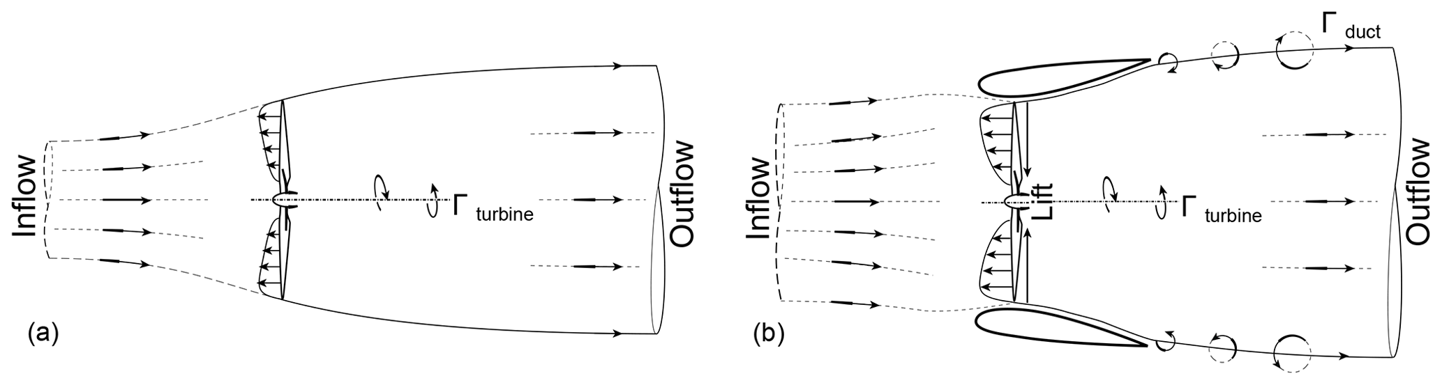
Figure 1Schematic of stream-tube model for a bare turbine (a) and DWT (b). The trailing vorticity in the wake is denoted by Γ.
Igra (1981) experimentally studied the effects of yaw on the performance of DWTs. Eight geometries were investigated using different duct profiles and an actuator disc (AD) model to represent the turbine. The eight configurations differed in the duct expansion ratio, i.e. the ratio of exit area of the duct to the turbine area. The AD with a thrust coefficient of approximately 0.5 was chosen. It was found that when the duct expansion ratio was less than 4.5, little or no difference in the power output was measured up to a yaw angle of ±30∘, while any further increase in yaw resulted in power reduction. On the other hand, when the duct expansion ratio was higher than 4.5, the generated power decreased even for small yaw angles. Igra (1981) explained that the yaw insensitivity for the low duct expansion ratio configurations is due to the lift force increase by the annular duct section. The author did not provide any explanation to further clarify the physics behind performance drop for large duct expansion ratio. On the same line, researchers from Grumman Aerospace tested a bare turbine and two DWT models (named Baseline DAWT and DAWT 45), varying the yaw angle up to 40∘ with increments of 10∘ (Gilbert and Foreman, 1983). Both the Baseline DAWT and DAWT 45 models showed a negligible change in the power up to a yaw angle of 30∘ and a drastic reduction in power at a yaw angle of 40∘. Surprisingly, the bare turbine also demonstrated no dependence on the yaw angle up to 30∘. They stated that this was due to the long centre-body configuration, similar in all three designs, that helped in channelling the incoming flow towards the upwind turbine blade and at the same time shielding the downwind turbine blade, thus offering an insensitivity to yaw. However, in a follow-up paper (Foreman and Gilbert, 1983) they stated that these yaw tests were inconclusive as to whether the yaw insensitivity was due to the centre-body effect or the duct geometry itself. More recently, Phillips et al. (2002) combined experimental and numerical analysis to study DWTs under yawed flow. They concluded that the power increase for a DWT in yawed flow can only be achieved with a slotted duct design (named Mo), with the added mass flow of air through the slot increasing the boundary layer flow control and preventing flow separation over the suction side (inner surface) of the duct under severe yaw misalignment. The above literature, due to the contrasting nature of the conclusions, lacks clarity regarding the aerodynamics of DWTs in yawed flow and particularly regarding the effect of the duct geometry on the aerodynamic performances. The present article aims to reignite the insights of Igra (1981), Foreman and Gilbert (1983), and Phillips et al. (2002) to study the effects of yaw on the performance of DWTs based on a numerical study.
In all the simulations presented in this article, the turbine is represented using a numerical actuator disc (AD) model, a method widely used to model the principal effects of turbines in a simplified manner. In the AD model, the turbine forces are assumed to be distributed evenly along the AD; hence, the influence of the blades is taken as an integrated quantity in the azimuthal direction. The effects of distributed forces for real turbine geometries are modelled using more sophisticated techniques like actuator line (Troldborg, 2009) or actuator surface (Shen et al., 2009) methods. Incorporating the real turbine geometries, which would necessarily have to be different for ducted and for bare operation, would confuse turbine and duct effects, preventing a proper analysis of DWTs in yawed flow. Thus, the AD approach is chosen deliberately for this investigation so as to study the impact of duct shapes and not the specific performance of a rotor within a duct. The effects of real turbines within different duct geometries are studied in a subsequent publication by the authors; see Dighe et al. (2020). The numerical AD method has been extensively validated; see for example Dighe et al. (2019a, b). The numerical AD model has been applied by Mikkelsen and Sørensen (2001) to study the flow on a horizontal-axis wind turbine in axial- and yawed-flow conditions. The numerical predictions agree reasonably well, both in axial- and yawed-flow conditions, when compared to the measurements on the Tjæreborg 2 MW field turbine. This model is also employed by Tongchitpakdee et al. (2005) to study yaw; the NASA Ames experiments of the National Renewable Energy Laboratory (NREL) Phase VI turbine are modelled for yaw angles from 0 to 45∘ to find reasonable agreement with the experiments.
The paper is organized as follows. Section 2 reports the non-dimensional coefficients adopted for characterizing the aerodynamic performance of the duct-AD model, both under non-yawed- and yawed-flow conditions. Section 3 describes the numerical settings and parameters with the description of the duct profiles chosen for the current investigation. Section 4 reports the numerical validation study. Insights on the aerodynamic performance coefficients with respect to yawed flow are discussed in Sect. 5, together with flow analysis. Finally, the most relevant results are summarized in the conclusions.
The turbine is modelled by a flat AD. The AD exerts a constant thrust force TAD, calculated across the AD surface SAD, which corresponds to a non-dimensional thrust force coefficient:
where ρ is the fluid density, and U∞ is the free-stream velocity.
To generate TAD, a uniform pressure drop is present across the AD surface, TAD= Δp × SAD. The pressure drop Δp is taken from experiments (Tang et al., 2016) and is given as an input parameter to the numerical simulations. The mean velocity across the AD radial plane, which is a function of AD thrust coefficient f(CT,AD), can be expressed by integrating the difference in the free-stream velocity component Ux across the AD surface:
Using Eqs. (1) and (2), the power coefficient for a bare AD reads
The subscript “o” has been adopted for quantities evaluated for the bare AD configuration.
For a duct-AD configuration, an additional thrust force exerted by the duct on the flow or vice versa appears. Then, the total thrust force T is the vectorial sum of the AD thrust force TAD and the duct thrust force TD, given by
The total thrust coefficient is then defined as
Note that the duct thrust coefficient is normalized with the AD area SAD to facilitate direct addition to the AD thrust coefficient for calculating the total thrust coefficient CT. Then, the mean velocity at the AD for a duct-AD model is a bivariate function of AD thrust coefficient and the duct thrust coefficient: UAD= f(CT). Similar to Eq. (3), the power coefficient for the duct-AD model, using SAD as the reference area, becomes
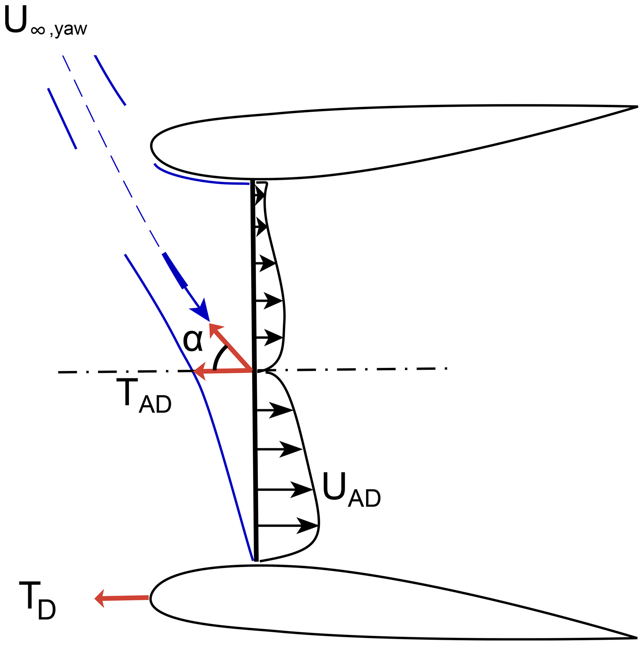
The power coefficient expression in Eq. (6) challenges the well-known Lanchester–Betz–Joukowsky limit of for maximum power coefficient obtainable for a HAWT. This should not be a surprising result since the mass flow for a given is larger than the mass flow without a duct. The additional thrust needed for the momentum balance is offered by the tilting of the lift force on the duct in the direction towards the incoming wind. The above relations are also valid for a DWT under yawed-flow conditions. Figure 2 shows the schematic of flow around the duct-AD model, where α is the yaw angle relative to the incident free-stream direction.

Figure 3Computational domain showing the boundary conditions employed (a). The lengths are normalized with the duct chord length c. Representative, not to scale. Computational grid surrounding the leading and trailing edge of the duct shown in panels (c) and (d), respectively.
In this study, a commercial CFD (computational fluid dynamics) solver ANSYS Fluent® is employed for solving the governing flow equations. The more sophisticated large-eddy simulation (LES) method, used in the context of DWT modelling (Dighe et al., 2020), is more likely to be more accurate in resolving complex flow features such as flow separation and vortex shedding. However, the LES method remains challenging for the parametric study presented here due to the limited computational capacity. Large flow separation regions are expected for DWTs in yawed flow. Flow solutions obtained using a steady Reynolds-averaged Navier–Stokes (RANS) formulation for DWTs with large yaw angles did not converge or even diverge. Moreover, the results presented by Phillips et al. (2008) show that the power predicted by the CFD simulations was significantly higher than that reached in the wind tunnel experiment. The overprediction can be attributed to a very high blockage correction factor used, while for the CFD results, the discrepancy can be attributed to the flow separation occurring inside the duct that was not captured computationally through the use of steady-state simulations and the choice of turbulence model (k−ϵ). Therefore, the solver utilizes the unsteady RANS (URANS) formulation to capture the asymptotic behaviour (quasi-steady state) of the flow. The k−ω shear stress transport (SST) model is employed for the turbulence closure scheme. Apsley and Leschziner (2000) investigated the ability of various second-order closure models to predict separated flows in a duct and compared them to experimental data. The k−ω SST model returns better predictions than the other second-order closure models with regards to approximating the unsteady flow in the velocity profiles of the duct. Moreover, Shives and Crawford (2012) investigated the application of different closure models for modelling ducted turbine flows. It was concluded that the k−ω SST model outperforms the other first and second-order closure models. A pressure-based coupled solver was selected with a second-order implicit transient formulation for improved accuracy. All solution variables were solved via a second-order upwind discretization scheme.
In order to evaluate the numerical duct-AD model in nearly unconstrained flow, the computational domain extends 12 c upstream and 24 c downstream, where c is the duct chord length. The distances are found to be safe choices to minimize the effects of blockage and uncertainty in the boundary conditions on the results; please refer to Appendix A. Using the finite-volume method, the computational domain is discretized spatially into a finite number of small control volumes known as grids. The grids have been generated using the commercial software ANSYS ICEM CFD. For the present computations, a C-grid structured zonal approach is chosen (see Fig. 3), which proved advantageous in the case of a curved boundary, i.e. the duct's leading edge. The C-shaped loop terminates in the wake region. The computational grid consists of quadrilateral cells with a maximum y+ value of ≈ 1 on the duct wall. A 3D grid is created by extruding the 2D grid using 100 grid points in the azimuthal direction ϕ with the surface grid extrusion technique (ANSYS, 2018). Boundary conditions are uniform velocity at the inlet, zero gauge static pressure at the outlet, and no-slip walls for duct surfaces. The numerical study is performed at a fixed Re of 4.5 × 10⁵. The influence of AD is included into the domain as an additional body force acting opposite to the direction of flow. This is achieved using a reverse fan boundary condition in ANSYS Fluent®. For a uniform thrust loading, the thrust force is given by
where is calculated from a semi-empirical relation of pressure drop curve and the velocity at the AD obtained from wind tunnel experiments. The fluid is air with fluid density ρ= 1.276 and dynamic viscosity Pa s. Values of free-stream velocity U∞ and turbulence intensity I are chosen for consistency with the wind tunnel experiments. To establish yawed-inflow conditions, the flow is rotated around the centre-line axis by yaw angle α for different test cases.
The simulations were advanced through time with a CFL (Courant–Friedrichs–Lewy) number of one, which resulted in a time step of approximately s. A typical converged 2D URANS solution with approximately 0.1 million mesh elements is obtained in roughly 30 min on a quad-core workstation desktop computer. The converged 3D URANS solution with approximately 10 million mesh elements is obtained in roughly 54 h on a quad-core workstation desktop computer.
For validating the numerical approach, experiments carried out by Igra (1981) on a duct-AD geometry (three-dimensional) are simulated. The experiments of Igra (1981) were conducted in the subsonic wind tunnel of the Israel Aerospace Industry (formerly Israel Aircraft Industry); this tunnel has a large test section, and it measures 3.6 m × 2.6 m.
A schematic of the cross-section geometry (named Model B) is shown in Fig. 4a. The longitudinal cross-section of the duct is a NACA 4412 airfoil. The leading edge of the duct is rotated by 2∘ with respect to the free-stream direction, resulting in a duct expansion ratio (area of duct exitarea of the AD) of 1.54. A uniformly loaded AD model with is used to represent the turbine; the value is based on the selection of the author for the experiments. The experimental data set consists of static pressure distribution at different axial and radial positions and forces generated by the duct surface for a range of flow angles. During the experiments, the inflow velocity was set at U∞=32 m s−1. Following Igra (1981), the wall interference and blockage correction can be ignored. The experimental data are reported in terms of the augmentation factor , which expresses the ratio between the power coefficient of the duct-AD model and the power coefficient of the bare AD model when both the models bear the same AD and similar operating conditions.

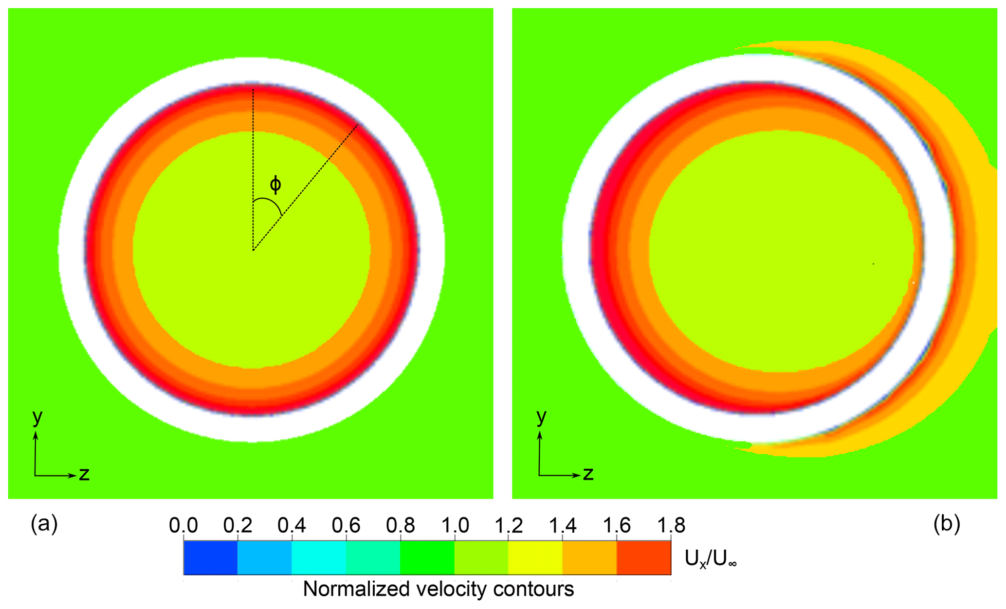
Figure 5Contours of time-averaged non-dimensional free-stream velocity Ux/U∞ measured at the AD location located in the y–z plane for Model B in (a) non-yawed inflow and (b) yawed inflow (α=10∘).
A good agreement between the CFD simulations and the experimental findings is found in Fig. 4b. The deviation between the CFD and the experimental findings increases with increasing values of α, especially for 2D URANS calculations.The differences in the 2D and 3D CFD results can be explained by looking at the flow field obtained using 3D URANS simulations. Figure 5 shows the time-averaged velocity contours of non-dimensional axial velocity in the y–z plane at the AD location for Model B in non-yawed- (left) and yawed-inflow (right) conditions. Time averaging is performed over the quasi-steady solutions after convergence is reached. Because of the yaw angle (α= 10∘), an asymmetric flow field is present; thus the velocity at the AD plane changes with the azimuthal angle Φ. Here, the azimuthal angle Φ is defined as positive in the clockwise direction when looking from upwind and is zero when oriented in the positive y direction; see Fig. 5 (left). The main difference between the two results is due to the fact that the CP (Eq. 6) obtained from 3D URANS simulations uses the azimuthally averaged streamwise velocity component, while the results from 2D simulations do not account for the gradual variation with Φ. However, as shown in the comparison, the three-dimensional azimuthal effects are negligible when comparing r. It is important to highlight that the maximum deviation between 2D URANS results and experimental findings is less than 5 % for α= ±15∘.
For an additional validation of the AD approach, numerical results obtained using 2D and 3D URANS are compared with the experimental study reported by Ten Hoopen (2009). The study was conducted using the full-scale DonQi® DWT model in non-yawed-inflow conditions (see Fig. 6). Experiments were conducted in the closed-loop open-jet (OJF) wind tunnel facility at Delft University of Technology. The average thrust coefficient of the turbine was measured in the experimental study to be 0.689; this value is chosen to model for the results presented. Figure 6 shows the comparison of the normalized free-stream velocity measured behind the turbine blade at in the radial direction y. Transition was not forced, but the experimental model has a noise damper (see Fig. 6) which acts as a rough surface that forces transition to turbulence; this has not been replicated numerically. The computed velocity profiles preserve the overall shape, with the relative difference calculated as lower than 10 %, which is within the experimental uncertainty and also attributed to the absence of discrete blades and their related effects such as tip vortices, wake rotation, and an accelerated mixing of the flow through the DWT with the external flow. An additional numerical verification exercise of the 2D URANS approach is performed, where the results are compared to a full-scale DWT numerical model. It is not reported herein for the sake of brevity; please refer to Appendix B.
The 2D URANS approach gives results of reasonable accuracy when compared to the 3D URANS approach. The computing cost issued by going from 2D URANS to 3D URANS does not justify the scope of the current study, where the effects of distributed AD loading, wake rotation, and divergence are totally ignored. Having said that, the 2D URANS approach combined with the numerical duct-AD model has been adopted for the results presented hereinafter.

Figure 6Comparison of dimensionless velocity profile vs. radius (at ) from the centre line between the experimental data and the CFD findings shown for the DonQi® DWT model in non-yawed-inflow conditions.
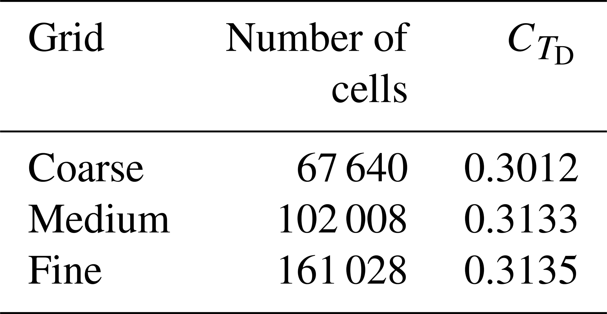
A grid independence analysis has been carried out for the 2D grid using three grid sizes, where the refinement factor in each direction is 1.5. The refinement factor is defined as the rate at which the grid size increases in the direction normal to the surface of the wall (duct surface). The duct thrust force coefficient is taken as reference for the convergence analysis. The results of the grid independence study are shown in Table 1. Convergence is reached for the medium refined grid, where the value fluctuates less than 0.0003 %, and a similar grid refinement is used in the numerical investigation hereinafter.
Table 1Grid statistics for the grid independence study of the reference case.

5.1 Duct geometries
Two duct geometries, shown in Fig. 7, with different longitudinal cross-sections (named DonQi® and DonQi® D5), are chosen for the current investigation. The selection is based on the duct shape parametrization study conducted by the authors (Dighe et al., 2019b). The parametrization procedure for duct shapes preserved the following geometric features: leading edge position (which defines the inlet area ratio), trailing edge position (which defines the exit area ratio), and inner side thickness (which preserves AD radius and clearance). This makes it ideal to isolate the effects of the duct cross-section on the aerodynamic performance of the duct-AD model in yaw. In the study, an optimal was obtained for both the duct geometries. This value is employed for the rest of the discussion.
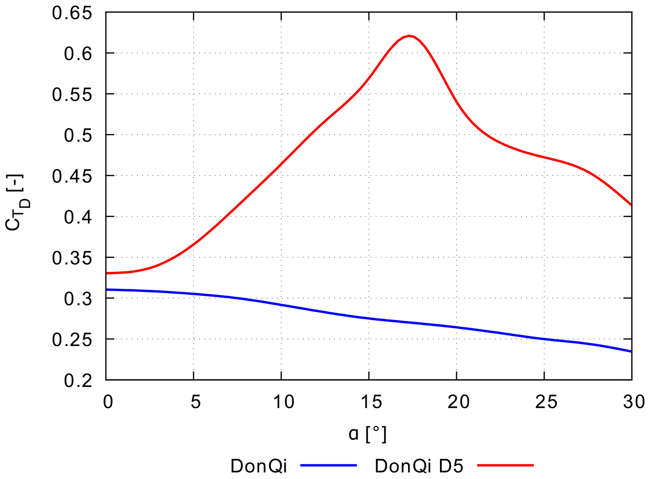
Figure 8Effect of yawed inflow on the duct thrust force coefficient for the two duct geometries. .
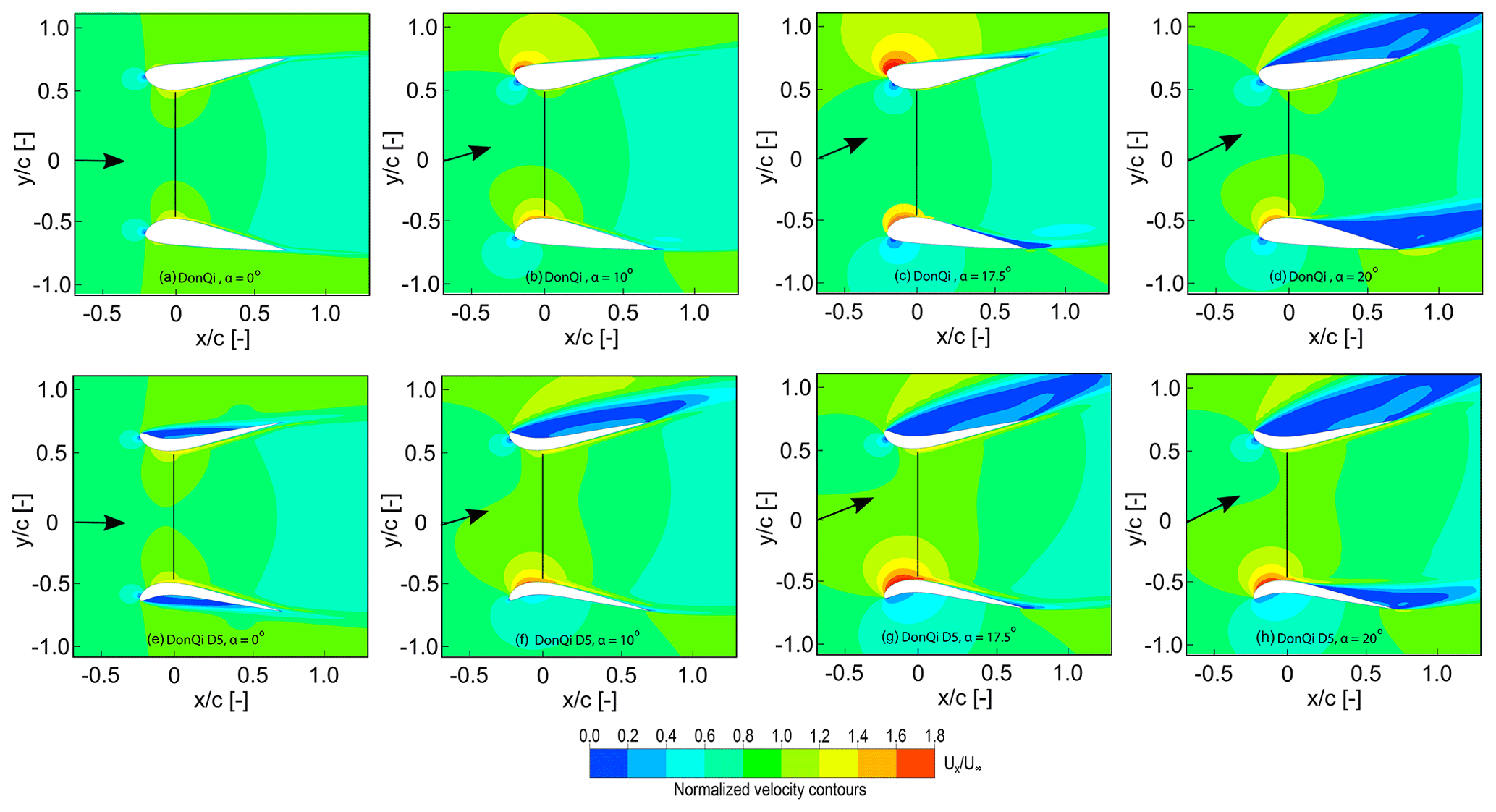
Figure 9Velocity contours coloured with streamwise normalized velocity. The results are depicted for the DonQi® duct-AD model (top) and DonQi® D5 duct-AD model (bottom), both bearing a constant 0.7.
5.2 Duct force coefficient
Figure 8 illustrates the variation in duct force coefficient as a function of yaw angle α obtained for the two duct geometries investigated in this study. Starting with the trend line for the DonQi® duct, it can be observed that decreases with increasing values of α. Conversely, for the DonQi® D5 duct, increases with increasing α. A local maximum at α=17.5∘ appears for the DonQi® D5 duct. The value of for the DonQi® D5 duct decreases for α beyond the local maximum.
The differences in the trend lines for the two duct geometries can be explained by looking at the flow field. Contours of non-dimensional free-stream velocity for both duct geometries are reported in Fig. 9a to h. A range of yaw angles have been tested; however, four yaw angles, i.e. α=0, 10, 17.5, and 20∘, are presented here for the sake of conciseness. For the DonQi® duct configuration, the low-pressure area, characterized by increased velocity, remains persistent inside and outside of the duct surfaces up to and including α=17.5∘. The low-pressure area, when seen outside of the duct surfaces, contributes negatively to the integrated duct thrust. For the DonQi® D5 duct configuration, however, the low-pressure area is limited on the inside of the duct surfaces, and the high-pressure area (characterized by reduced velocity) appears on the outside of the duct surfaces. The high-pressure area is the result of the duct profile camber and is accompanied by flow separation, which adds positively to the duct thrust (see Fig. 8). At α= 20∘, where both DonQi® and DonQi® D5 configurations are completely stalled, the resultant is higher for the DonQi® D5 duct. This is because the impact of stalled flow on the pressure side of the windward airfoil for DonQi® D5 is larger since the stagnation pressure acts on the concave duct surface in comparison to the DonQi® duct surface, which is more convex. Hence, the resultant for the DonQi® D5 duct is much higher when compared with the DonQi® duct (see Fig. 8) even though the general flow pattern in Fig. 9 (α=20∘) looks quite similar.
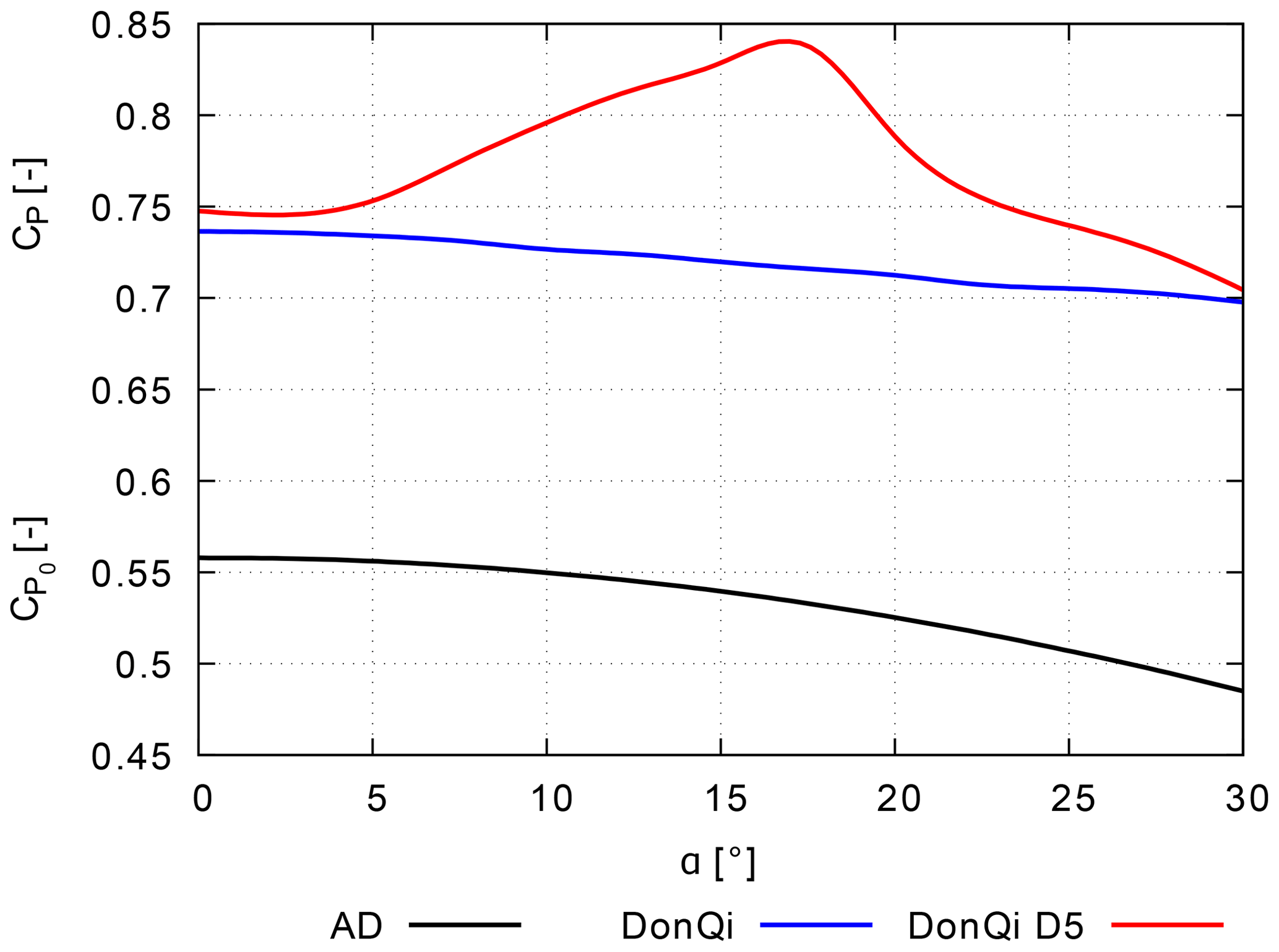
5.3 Power coefficient
Figure 10 represents the power coefficient CP for the two duct configurations as a function of yaw angle α. For the sake of completeness, for a bare AD is plotted alongside the CP for the duct AD. The figure shows that CP is higher than for all values of α. Comparing Figs. 8 and 10, the CP trends correspond to the trends. The larger the , the higher the CP reached and vice versa. Similar to the trend for DonQi® D5, a maximum CP ≈ 0.84 is obtained for the DonQi® D5 duct at α= 17.5∘; thereafter any further increase in α results in a CP drop. This also explains the experimental observations from Igra (1981), where a drop in the power coefficient for the duct-AD models with a large duct expansion ratio was observed. For a high duct expansion ratio, the likelihood of flow to separate from the inner walls of the duct increases (Abe and Ohya, 2004), thus lowering the and CP values for a given duct-AD model.
The present article reignites the insights of Igra (1981), Foreman and Gilbert (1983), and Phillips et al. (2002) to study the effects of yaw on the performance of DWTs. To this aim, two-dimensional numerical calculations using URANS simulations are performed. Based on the existing studies conducted by Dighe et al. (2019b, 2020), two duct geometries with different cross-section camber (named DonQi® and DonQi® D5) are chosen. To validate the numerical approach, comparison of the numerical results with the experimental data is reported. Of the two duct geometries investigated, the DonQi® D5 duct configuration returns a gain in CP up to and including a yaw angle α=17.5∘; thereafter any further increase in α results in the CP drop. In contrast, CP of the DonQi® duct configuration drops for α>0∘. Flow field analysis pointed out that the aerodynamic performance of DWTs in yawed flow depends on the distinct shape of the duct under consideration. The high duct profile camber acts as a flow-conditioning device and delays duct wall flow separation inside of the duct for a broad range of yaw angles. This phenomenon is characterized by a rapid increase in duct thrust force coefficient and ultimately the CP for the DonQi® D5 configuration in yaw. For the investigation presented here, a constant AD loading 0.7 is chosen based on the optimization study presented in Dighe et al. (2019b). Future studies can investigate the effects of yaw on the performance of DWTs for a range of values.
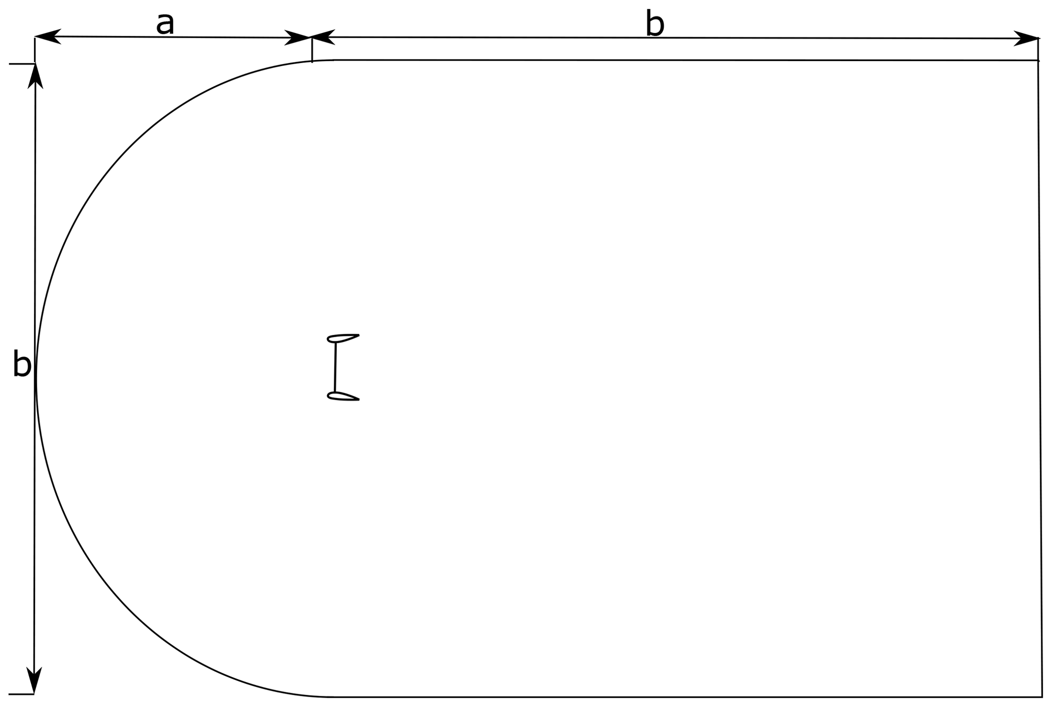
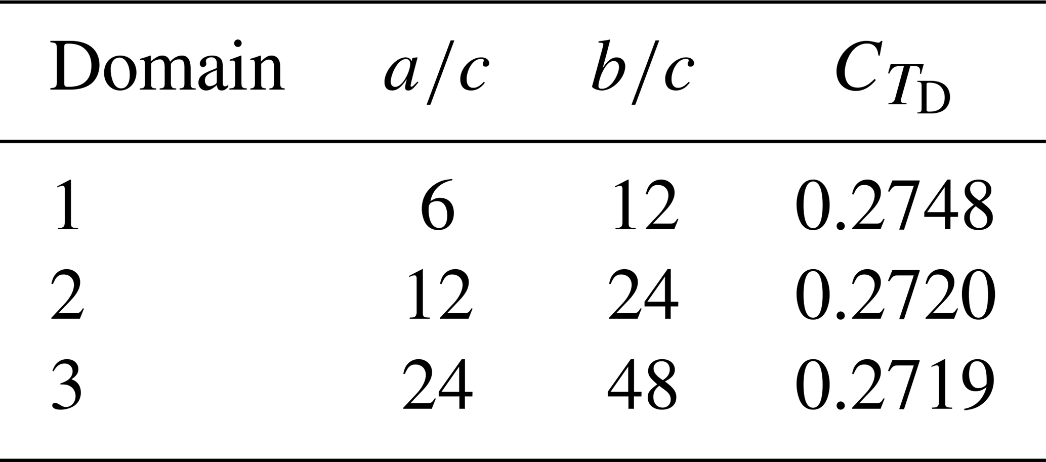
A major underlying factor that influences the accuracy and computational expense of CFD simulations is the size of the computational domain. For our current investigation, the size of the computational domain is defined by two variables, a and b (see Fig. A1), where a is the upstream domain length from the AD location, and b is the total height of the domain and also the downstream domain length from the AD location; both the variables are normalized by the duct chord length c. The study is performed using the baseline DonQi® duct-AD model at a yaw angle of 15∘.
The effect of computational domain sizes on the numerical prediction of is shown in Table A1. The unsteady simulations collect data, which are oscillating in time; time-averaged values obtained in a quasi-steady state are shown here. The values for domains 2 and 3 are almost identical, representing nearly unconfined conditions. The negligible difference can be attributed to the iterative convergence error or the computer round-off error. Domain 2 is chosen for the cases presented in this article.
Three-dimensional lattice Boltzmann very-large-eddy simulations (LB-VLESs) of DWTs, where the rotor is simulated, in axial- and yawed-inflow conditions form the reference for the verification of the numerical approach presented in this article. For a detailed description of the LB-VLES approach, computational set-up, and operating conditions, the reader can refer to Dighe et al. (2020). The baseline DonQi® DWT model is simulated for α= 0 and 7.5∘. The free-stream velocity is U∞= 5 m s−1, which corresponds to a Reynolds number Re= 3.31 × 10⁵. Based on a previous study by Avallone et al. (2020), the resulting average rotor thrust coefficient equals 0.8; this value is adopted for specifying the input for the AD model.
Figure B1 examines the streamwise velocity component as a function of radial position using the two numerical approaches under both non-yawed- and yawed-flow conditions. Before beginning this discussion, it must be stressed that the LB-VLES approach consists of turbine blades that are connected to a hub (upstream) and a nacelle (downstream). This geometric feature is not included in the duct-AD model; see Fig. B2c and d. Despite this source of uncertainty in the AD modelling approach, viz. absence of discrete blade (including hub and nacelle) effects and wake rotation, the overall computed trends show good agreement. As a testimony to model skewed wake, as seen in Fig. B2d, the 2D URANS duct-AD approach exhibits a strong potential to implicitly model the flow around a DWT in yaw. The proposed simplified approach thus captures first-order flow physics; for higher-order effects, the blade-shape-resolving models will be well suited.
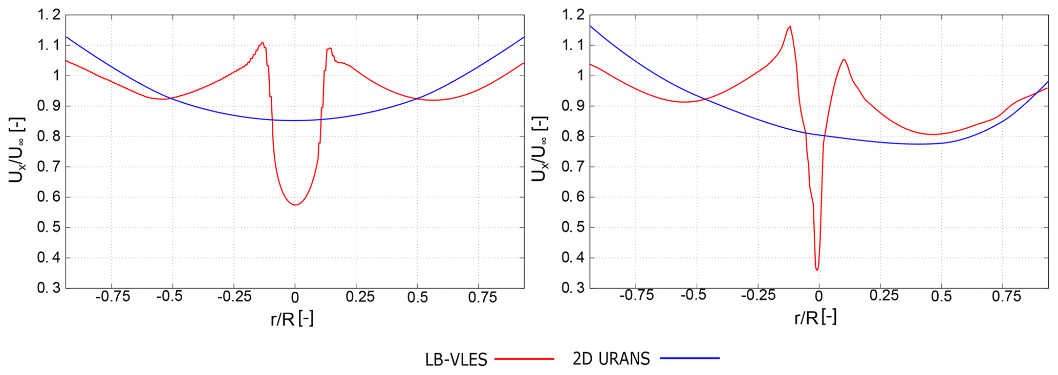
Figure B1Radial distribution of streamwise velocity located just aft of the turbine–AD plane.

Figure B2Contours of instantaneous streamwise velocity in the x–y plane for (a) DonQi® at α=0∘ using the LB-VLES approach, (b) DonQi® at α= 7.5∘ using the LB-VLES approach, (c) DonQi® at α= 0∘ using the 2D URANS approach, and (d) DonQi® at α= 7.5∘ using the 2D URANS approach.
The supplement data related to this article were produced using a commercial CFD software Ansys. The authors would share the geometry, case files, and the data files, which could be later made available to the interested readers through a DOI.
VD compiled the literature review, set up and performed the CFD simulations, and wrote the bulk of the paper. DS performed the CFD simulations, post-processed the cases, and contributed towards writing this paper. FA reviewed the paper and carried out modifications in different sections of this paper. GvB participated in regular group discussions, revisions, and funding acquisition.
The authors declare that they have no conflict of interest.
Publisher’s note: Copernicus Publications remains neutral with regard to jurisdictional claims in published maps and institutional affiliations.
This article is part of the special issue “Wind Energy Science Conference 2019”. It is a result of the Wind Energy Science Conference 2019, Cork, Ireland, 17–20 June 2019.
The authors would like to acknowledge Ozer Igra for providing the experimental data that have contributed to part of the numerical validation reported in this paper. The research is supported by the STW organization (grant no. 12728).
This research has been supported by the STW (grant no. 12728).
This paper was edited by Katherine Dykes and reviewed by Paul van der Laan and four anonymous referees.
Abe, K., Nishida, M., Sakurai, A., Ohya, Y., Kihara, H., Wada, E., and Sato, K.: Experimental and numerical investigations of flow fields behind a small wind turbine with a flanged diffuser, J. Wind Eng. Ind. Aerod., 93, 951–970, 2005. a
Abe, K.-I. and Ohya, Y.: An investigation of flow fields around flanged diffusers using CFD, J. Wind Eng. Ind. Aerod., 92, 315–330, 2004. a
ANSYS, I.: ANSYS ICEM CFD user’s manual 18.0, ANSYS Inc., Canonsburg, Pennsylvania, USA, 2018. a
Apsley, D. and Leschziner, M.: Advanced turbulence modelling of separated flow in a diffuser, Flow, Turbulence and Combustion, 63, 81–112, https://doi.org/10.1023/A:1009930107544, 2000. a
Avallone, F., Ragni, D., and Casalino, D.: On the effect of the tip-clearance ratio on the aeroacoustics of a diffuser-augmented wind turbine, Renew. Energ., 152, 1317–1327, 2020. a
Dighe, V. V., Avallone, F., Igra, O., and van Bussel, G.: Multi-element ducts for ducted wind turbines: a numerical study, Wind Energ. Sci., 4, 439–449, https://doi.org/10.5194/wes-4-439-2019, 2019a. a
Dighe, V. V., de Oliveira, G., Avallone, F., and van Bussel, G. J.: Characterization of aerodynamic performance of ducted wind turbines: A numerical study, Wind Energy, 22, 1655–1666, https://doi.org/10.1002/we.2388, 2019b. a, b, c, d
Dighe, V. V., Avallone, F., and van Bussel, G.: Effects of yawed inflow on the aerodynamic and aeroacoustic performance of ducted wind turbines, J. Wind Eng. Ind. Aerod., 201, 104174, https://doi.org/10.1016/j.jweia.2020.104174, 2020. a, b, c, d
Dupont, E., Koppelaar, R., and Jeanmart, H.: Global available wind energy with physical and energy return on investment constraints, Appl. Energ., 209, 322–338, 2018. a
Foreman, K. and Gilbert, B.: A Free Jet Wind Tunnel Investigation of DAWT Models, Grumman research and development Center Report to SERI, RE-668 (SERI/TR 01311-1), Grumman Aerospace Corp., Bethpage, NY, USA, 1983. a, b, c
Gielen, D., Boshell, F., Saygin, D., Bazilian, M. D., Wagner, N., and Gorini, R.: The role of renewable energy in the global energy transformation, Energy Strateg. Rev., 24, 38–50, 2019. a
Gilbert, B. and Foreman, K.: Experiments with a diffuser-augmented model wind turbine, J. Energ. Resour.-ASME, 105, 46–53, 1983. a, b
Igra, O.: Research and development for shrouded wind turbines, Energ. Convers. Manage., 21, 13–48, 1981. a, b, c, d, e, f, g, h, i, j
Khamlaj, T. and Rumpfkeil, M.: Theoretical Analysis of Shrouded Horizontal Axis Wind Turbines, Energies, 10, 38, https://doi.org/10.3390/en10010038, 2017. a
de Vries, O.: Fluid dynamic aspects of wind energy conversion, Tech. rep., Advisory Group for Aerospace Research and Development NEUILLY-SUR-SEINE, France, 1979. a
Mikkelsen, R. and Sørensen, J.: Yaw analysis using a numerical actuator disc model, in: Proceedings of 14th IEA Symposium on the Aerodynamics of Wind Turbines, FFA, 14th IEA Symposium on the Aerodynamics of Wind Turbines, 4–5 December 2000, 2001. a
Phillips, D., Richards, P., and Flay, R.: CFD modelling and the development of the diffuser augmented wind turbine, Wind Struct., 5, 267–276, 2002. a, b, c
Phillips, D., Richards, P., and Flay, R.: Diffuser development for a diffuser augmented wind turbine using computational fluid dynamics, Department of Mechanical, Engineering, the University of Auckland, New Zealand, 2008. a
Shen, W. Z., Zhang, J. H., and Sørensen, J. N.: The actuator surface model: a new Navier–Stokes based model for rotor computations, J. Sol. Energ.-T. ASME, 131, 011002, https://doi.org/10.1115/1.3027502, 2009. a
Shives, M. and Crawford, C.: Developing an empirical model for ducted tidal turbine performance using numerical simulation results, P. I. Mech. Eng. A-J. Pow., 226, 112–125, 2012. a
Tang, J., Avallone, F., and van Bussel, G.: Experimental study of flow field of an aerofoil shaped diffuser with a porous screen simulating the rotor, International Journal of Computational Methods and Experimental Measurements, 4, 502–512, 2016. a
Ten Hoopen, P.: An Experimental and Computational Investigation of a Diffuser Augmented Wind Turbine: with an application of vortex generators on the diffuser trailing edge, MS thesis, TU Delft, the Netherlands, 2009. a
Tongchitpakdee, C., Benjanirat, S., and Sankar, L.: Numerical simulation of the aerodynamics of horizontal axis wind turbines under yawed flow conditions, J. Sol. Energ.-T. ASME, 127, 464–474, 2005. a
Toshimitsu, K., Nishikawa, K., Haruki, W., Oono, S., Takao, M., and Ohya, Y.: PIV measurements of flows around the wind turbines with a flanged-diffuser shroud, J. Ther. Sci., 17, 375–380, 2008. a
Troldborg, N.: Actuator line modeling of wind turbine wakes, PhD thesis, Technical University of Denmark, Denmark, 2009. a
Valyou, D. and Visser, K.: Design considerations for a small ducted wind turbine, in: Journal of Physics: Conference Series, 1452, 012019, IOP Publishing, 2020. a
Van Bussel, G.: The science of making more torque from wind: Diffuser experiments and theory revisited, J. Phys. Conf. Ser., 75, 120–10, 2007. a, b
Werle, M. and Presz, W.: Ducted wind/water turbines and propellers revisited, J. Propul. Power, 24, 1146–1150, 2008. a
- Abstract
- Introduction
- Duct – AD flow model
- Methodology and computational set-up
- Numerical verification and validation
- Results and discussion
- Conclusions
- Appendix A: Domain blockage study
- Appendix B: Numerical verification of the duct-AD model
- Code availability
- Author contributions
- Competing interests
- Disclaimer
- Special issue statement
- Acknowledgements
- Financial support
- Review statement
- References