Seasonal effects in the long-term correction of short-term wind measurements using reanalysis data

Measure–correlate–predict (MCP) approaches are often used to correct wind measurements to the long-term wind conditions on-site. This paper investigates systematic errors in MCP-based long-term corrections which occur if the measurement on-site covers only a few months (seasonal biases). In this context, two common linear MCP methods are tested and compared with regard to accuracy in mean, variance, and turbine energy production – namely, variance ratio (VR) and linear regression with residuals (LR). Wind measurement data from 18 sites with different terrain complexity in Germany are used (measurement heights between 100 and 140 m). Six different reanalysis data sets serve as the reference (long-term) wind data in the MCP calculations. All these reanalysis data sets showed an overpronounced annual course of wind speed (i.e., wind speeds too high in winter and too low in summer). However, despite the mathematical similarity of the two MCP methods, these errors in the data resulted in very different seasonal biases when either the VR or LR methods were used for the MCP calculations. In general, the VR method produced overestimations of the mean wind speed when measuring in summer and underestimations in the case of winter measurements. The LR method, in contrast, predominantly led to opposite results. An analysis of the bias in variance did not show such a clear seasonal variation. Overall, the variance error plays only a minor role for the accuracy in energy compared to the error in mean wind speed. Besides the experimental analysis, a theoretical framework is presented which explains these phenomena. This framework enables us to trace the seasonal biases to the mechanics of the methods and the properties of the reanalysis data sets. In summary, three aspects are identified as the main influential factors for the seasonal biases in mean wind speed: (1) the (dis-)similarity of the real wind conditions on-site in correlation and correction period (representativeness of the measurement period), (2) the capability of the reference data to reproduce the seasonal course of wind speed, and (3) the regression parameter β₁ (slope) of the linear MCP method. This theoretical framework can also be considered valid for different measurement durations, other reference data sets, and other regions of the world.

1 Introduction

An extensive measurement campaign generally constitutes an essential part of wind resource assessment and, therefore, of a successful wind energy project. In most cases, these measurements provide around 1 year of wind data at the site of interest (Lackner et al., 2008). Inter-annual variations in wind speed are reported to vary by between 4 % and up to 10 % (e.g., Corotis, 1976; Justus et al., 1979; Klink, 2002), depending on the respective site; hence, the measured wind data usually do not represent the long-term wind conditions. This aspect becomes even more momentous when the energy in the wind is considered, which has been reported to vary by 6 % (Pryor et al., 2018) up to 20 % or even 30 % (Corotis, 1976; Albrecht and Klesitz, 2006; Pryor et al., 2006) from year to year. To account for this issue, a long-term correction is performed.

For this purpose, reference data are needed, which should be available for a long-term period of one to two decades (Lackner et al., 2008; Carta et al., 2013; Liléo et al., 2013) and show a high degree of similarity to the measured wind data (e.g., a high correlation coefficient of measured and reference data).

Over the recent past, reanalysis data gained more and more popularity in the wind industry and are now used extensively in wind resource assessment (Miguel et al., 2019; Ramon et al., 2019). Reanalysis data sets are produced using numerical weather simulations with a fixed state-of-the-art model and assimilating historical weather data. In contrast to models used for weather prediction, which are often updated and changed during operations, they therefore provide temporally consistent data sets over periods of up to several decades. Different types of reanalysis data are available, ranging from (often freely available) global data sets (e.g., MERRA-2 by NASA, NASA, 2019; ERA5 by ECMWF, CDS, 2018) to mesoscale reanalyses, which are generally not free of charge but provide higher spatial resolution.

A statistical procedure relating the reference data to the measured data is performed to derive a correction function. In this context measure–correlate–predict (MCP) approaches have evolved to become a standard tool for wind farm developers (Carta et al., 2013). These methods model a statistical relationship between the time series of the reference and the measurement data. Afterwards, the relationship is applied to the long-term reference data, providing the long-term wind conditions. The relationship between reference and target data, therefore, is assumed not to be time-dependent, i.e., valid in the correlation period as well as in the correction period.

Numerous MCP methods are used in modern wind resource assessment applications. They range from simple linear models (e.g., García-Rojo, 2004; Rogers et al., 2005a; Romo Perea et al., 2011; Weekes and Tomlin, 2014a) to complex machine learning approaches like neural networks (e.g., Bass et al., 2000; Albrecht and Klesitz, 2006; Bilgili et al., 2007; Velázquez et al., 2011; Zhang et al., 2014). The investigation and comparison of different MCP approaches has been subject to a large amount of studies. Carta et al. (2013) present an extensive review on existing MCP methods applied in wind resource assessment and related research fields. They concluded that, by far, the most commonly used MCP methods in the wind industry are based on linear approaches. Other studies confirm this observation and underline the benefit of the simplicity of linear MCP methods for use in wind energy applications (e.g., Sørensen et al., 2011; Weekes and Tomlin, 2014c; Weekes et al., 2015). In a round-robin experiment in Germany in 2018 it was found that 24 of 29 consultants used linear correlation methods, which mostly outperformed more complicated approaches (Basse et al., 2018).

In order to enable a precise determination of the relationship between measurement and reference data, a sufficient amount of measurement data is necessary; that is, the concurrent period needs to be long enough. Various studies have been presented in which the question is addressed of how long the time span covered by the measurement should be. In general, it is recommended to be at least 1 year (Carta et al., 2013), while the use of complete years is important as an uneven representation of different months increases the uncertainty (Taylor et al., 2004; Liléo et al., 2013). As a consequence of such studies, an amount of 12 months of measurement is recommended or even a mandatory minimum duration due to technical guidelines and standards such as FGW e.V. (2020), IEC (2017), or MEASNET (2016).

From an economic perspective, though, there is a strong desire to reduce the duration of the measurement in order to save time and money (Carta et al., 2013). This is especially true with the increasing popularity of lidar measurements, which have a high mobility and low installation costs compared to classical measurement masts with comparatively high running costs. Moreover, an estimate of the wind conditions on-site is often of interest for the wind park planner before the measurement campaign is completed. In all such cases, a smaller number of wind data need to be dealt with, and a long-term correction is performed based on wind measurement data which comprise much less than a year.

However, seasonal effects occur when the measurement does not cover all seasons (Rogers et al., 2005a; Saarnak et al., 2014; Weekes and Tomlin, 2014a, b, c), resulting in a dependence of the estimated energy yield on the period in which the measurement is conducted. These can induce systematic deviations and, thus, increase the uncertainty of the resource assessment significantly. Therefore, understanding seasonal patterns in long-term correction and their relation to data sources and the choice of the MCP method is of high interest for the wind industry.

Several studies have investigated the accuracy of a long-term correction (LTC) of short-term wind measurements in dependence of the measurement duration (e.g., Taylor et al., 2004; Rogers et al., 2005a, b; Romo Perea et al., 2011; Weekes and Tomlin, 2014c; Weekes et al., 2015; Miguel et al., 2019). While in some of these, seasonal effects are broadly addressed, to the authors' knowledge there is a lack of scientific publications which give profound explanations for seasonal patterns in biases of the LTC. This paper investigates seasonal effects and related biases in wind speed (mean and variance) and annual energy yield in the LTC induced by short (3 months) measurement periods. Motivated by their relevance for practical use, two linear MCP methods are applied and compared: linear regression with residuals (Weekes and Tomlin, 2014a) and the variance ratio method (Rogers et al., 2005a). First, theoretical considerations are developed to assess the impact of varying statistical relationships between the measurement and the reference data in the short-term period when compared to the long-term period. In a second step, wind measurement data from 18 sites in Germany and six different reanalysis data sets are used to assess the significance and magnitude of seasonal effects in the LTC. Interrelations of the seasonal effects with properties of the reference data and the correlation method are analyzed both theoretically and experimentally.

2 Measurement and reanalysis data used in this study

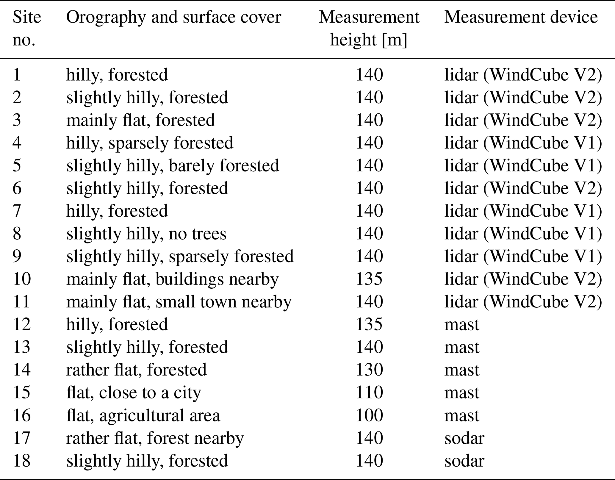
Table 1 presents an overview of the measurement campaigns used in this study. All sites are located in Germany; the complexity of the sites ranges from flat agricultural areas to the hilly low mountain ranges in Central Germany (one of the complex sites is described in Pauscher et al., 2018). For all sites a time series of an entire year for a height level between 100 and 140 m is available, representing typical hub heights of modern wind turbines. The data were collected by profiling lidar (light detection and ranging; see, e.g., Emeis et al., 2007) of type Leosphere WindCube V1 and V2 (Leleu, 2019), sodar (sound detection and ranging; see, e.g., Bradley, 2008), or mast measurements. The 1-year periods are distributed relatively homogeneously between May 2013 and April 2019; only the year 2016 may be judged slightly overrepresented (with 8 of the 18 sites covering at least a few months of the year 2016). The measurement data were collected at a temporal resolution of 10 min and then averaged to hourly values (centered at the full hour) to comply with the typical temporal resolution of the reanalysis data (see below). The availability of the measurement data is higher than 80 % at all sites with more than 90 % data availability at 14 sites. All data gaps are smaller than 100 consecutive hours except for a single site (site 17 in Table 1), where approx. 10 d of data are missing in winter (overall data availability for this site: 95 %).

Table 1 Details of the measurement sites. The duration of the individual measurements is exactly 1 year. The measurements were carried out between May 2013 and April 2019.

The following six different reanalysis data sets serve as reference data in the MCP calculations.

1. MERRA-2 (GMAO, 2015). The Modern-Era Retrospective Analysis for Research and Applications Version 2 (MERRA-2) is based on global numerical weather analyses of the US National Aeronautics and Space Administration (NASA). The data are available as 1 h time series since 1980 for a height of 50 m and a spatial resolution of $\mathrm{0.5}{}^{\circ }\times \mathrm{0.66}{}^{\circ }$. The time stamps refer to average hourly values centered at 00:30, 01:30 UTC, etc. In order to obtain comparability with the other reanalysis data sets and consistency in temporal terms, these were interpolated to values centered at the full hour.

2. ERA5 (Hersbach et al., 2020). The data set is calculated at the European Centre for Medium-Range Weather Forecasts (ECMWF) and provided by the Copernicus Climate Change Service. The ERA5 data represent the follow-up data set to the ERA-Interim reanalyses of the ECMWF. The spatial resolution of the ERA5 data is approx. 31 km (≈0.28^∘). Long-term series of this data set are available for 100 m above ground in an hourly resolution. In contrast to the MERRA-2 data, these data are instantaneous values instead of averaged wind speeds (centered at the full hour).

3. EMD-ConWx (EMD, 2020a). This data set is created using the WRF model (Weather Research and Forecasting Model; see, e.g., Powers et al., 2017) and is provided by EMD International A/S from Denmark. It is based on the ERA-Interim reanalysis data of the ECMWF, refined to a resolution of 3 km. The temporal resolution of the long-term time series is 1 h (instantaneous values centered at the full hour). Wind data are provided at heights of 10, 25, 50, 75, 100, 150, and 200 m.

4. EMD-WRF Europe+ (EMD, 2020b). This data set is a further development of the EMD-ConWx data. The ERA5 reanalysis data have replaced the ERA-Interim data, while spatial resolution and temporal properties have not changed. Wind data are provided at the same heights as in EMD-ConWx and six additional heights up to 4000 m.

5. anemosM2: anemos Windatlas based on MERRA-2 (anemos, 2020a, c). Similar to the EMD data sets, these data are created based on a downscaling of global reanalysis data (here MERRA-2) using the WRF model (version 3.7.1) to a resolution of 3 km. In contrast to the other models, anemos uses statistical post-processing based on measurement data, known as remodeling, to improve the simulation results. Furthermore, additional downscaling of the data from the 3 km grid to the specific site is applied. The heights of the wind data are generally freely selectable between 40 and 200 m; for the analysis in this study, wind data at 100 and 140 m were provided.

6. anemosE5: anemos Windatlas based on ERA5 (anemos, 2020b, c). This data set is similar to the anemosM2 but uses ERA5 data. Furthermore, in the course of the remodeling, a seasonal correction is performed, i.e., biases in the annual cycle of the ERA5 data are corrected before the statistical downscaling is implemented. The goal is to better capture the seasonal behavior of the wind conditions. Additionally, a more precise consideration of the roughness at the respective site represents a further difference to the anemosM2 data. Both the magnitude of the seasonal corrections and the modifications on roughness constitute a trade secret of anemos (Martin Schneider, anemos GmbH, personal communication, January 2021).

It should be noted that both the anemosM2 and anemosE5 models generally provide a temporal resolution of 10 min. In order to guarantee comparability of the results, these were averaged to 1 h, ensuring the same temporal resolution for all reanalysis data sets.

In general, reanalysis data are modeled for different locations on a geographical grid. In this study, data were selected from the grid point closest to the respective site. For data sets 3–6 data at more than one height level were provided. In these cases, the data at the height closest to the measurement were used (i.e., 100 and 150 m for EMD-ConWx and EMD-WRF Europe+, and 100 and 140 m for the two anemos data sets). For the MERRA-2 and ERA5 data sets the data at the given height (i.e., 50 and 100 m, respectively) were used; i.e., no vertical extrapolation (or interpolation) was performed in this study.

3 Methodology

This study compares wind speed statistics as observed over different periods in the investigated data – namely short-term data and long-term data. For this purpose, the convention is applied that capital letters are used for long-term variables (e.g., the long-term corrected wind speed), while parameters in lowercase letters represent data from the short-term period. The subscript labels “meas”, “rea”, and “corr” refer to measurement, reanalysis, and corrected data, respectively.

3.1 Selection of short-term periods and procedure of long-term correction

In this study, short-term periods with a duration of 90 consecutive days are investigated. For the selection of these short-term periods, a sliding window algorithm with an increment of 3 d is used; i.e., the first 90 d period starts on 1 January, the second on 4 January, etc. When this sliding window reaches the end of the period of the original measurement campaign, the data from the beginning of the data set are appended. This ensures that all seasons are considered equally. In this way, one hundred twenty-two 90 d measurement periods were investigated for all sites. This procedure is applied equally to measurement and reanalysis data, guaranteeing that the respective time series values match consistently.

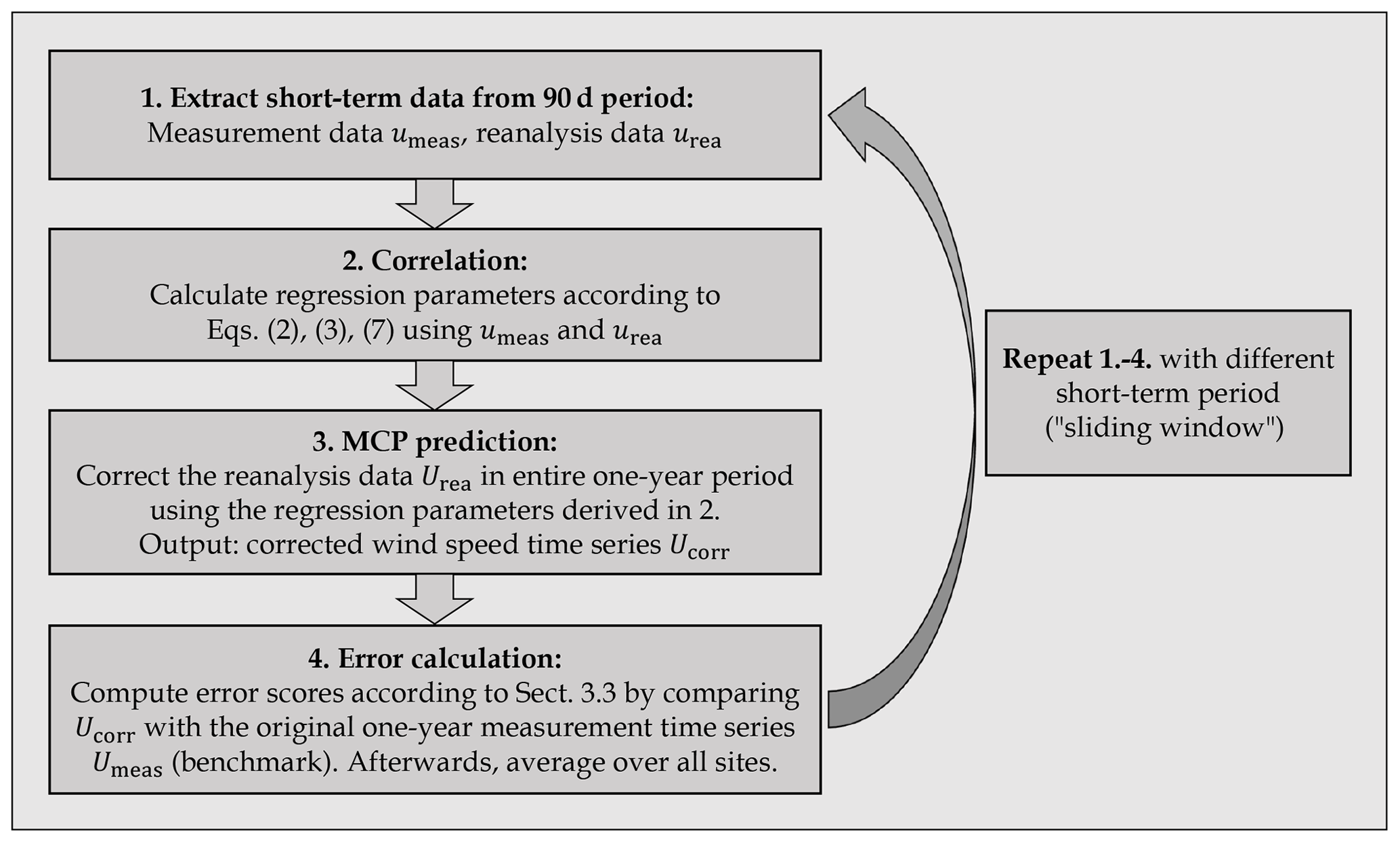
Figure 1 Illustration of the general procedure used in this study regarding the MCP predictions. After extracting the short-term data of measured (u_meas) and reanalysis (u_rea) data, a correlation function of these two wind speed time series is determined. This relationship is used to correct the reanalysis data in the entire 1-year period U_rea. Finally, the obtained corrected data U_corr is compared to the actually measured values (benchmark) U_meas in order to estimate the accuracy. This procedure is done with all one hundred twenty-two 90 d periods, all sites, and all reanalysis data sets separately.

In a first step, the data in each of the 90 d periods are investigated with respect to, e.g., mean and variance of wind speed (Sect. 5.1–5.3). In this way, the temporal variations of the wind climate can be analyzed. Furthermore, the performance of the reanalysis data in reproducing the measured wind conditions is evaluated. Overall, this provides the basis for the further investigations of the seasonal effects in the long-term correction of short-term wind measurements.

Secondly, MCP predictions are performed. Applying the linear MCP methods described below in Sect. 3.2, regression parameters are determined by deriving a statistical relationship between the measurement and reanalysis wind speed time series from the short-term period. Afterwards, the reanalysis data are adjusted to the entire 1-year period for which measurement data are available. This is done by using the previously derived statistical relationship. Finally, the corrected data are compared to the measured 1-year data (benchmark), and error scores are derived (see Sect. 3.3). The general procedure is illustrated in Fig. 1.

The results, therefore, do not represent the overall errors (or uncertainty) of an LTC in general, which is usually performed over a period of 10 years or more (Lackner et al., 2008; Carta et al., 2013; Liléo et al., 2013). Instead, the analysis provides findings on systematic errors (seasonal biases) which emerge due to the reduction of the measurement duration from 1 year to 3 months.

The procedure as depicted in Fig. 1 is carried out for each measurement site and for each reanalysis data set separately. In order to derive robust, conclusive findings, the individual results obtained at the 18 sites were averaged arithmetically, resulting in one set of statistics (e.g., error scores) for each reanalysis data set and each 90 d measurement period.

It should be noted that in practical applications, a sectorwise regression is often performed for an LTC of measurement data comprising a whole year. This means that the regression parameters are calculated separately for different wind direction bins, which allows taking the effects of terrain on wind flow into account. This can be important especially in a complex environment (López et al., 2008). For the shorter 3-month periods, sectorwise binning, however, generally yielded slightly worse results in this study (presumably due to low data coverage in the different direction sectors). This procedure is, therefore, not applied here. It is acknowledged, though, that in some specific cases a sectorwise approach can be a reasonable choice for an LTC of short-term measurements nevertheless.

When a correction is performed, the MCP methods may generate a few negative wind speed values. In this study, these values were set to zero.

As mentioned in the introduction, the correlation coefficient of site and reference data should be evaluated before a long-term correction is performed. It is obvious that the correlation coefficient is lower when considering short-term periods (this will shortly be addressed in Sect. 5.4.2). In most combinations of reanalysis and site data, the correlation coefficient was $r_{\mathrm{rea},\mathrm{meas}}>\mathrm{0.65}$ throughout, despite the small amount of only 90 d of data. Only in the case of the EMD-ConWx and EMD-WRF Europe+ data sets, values of less than 0.5 were observed in summer periods at some sites. This should be considered when assessing the results. However, it should be noted that this work intends to analyze the effects of shortening the measurement campaign for MCP approaches. Therefore, periods with low correlation coefficients are not excluded, but the effects of the correlation coefficient are explored in several sections (Sects. 4.3, 5.2, and 5.4.2 in particular).

3.2 Long-term correction: measure–correlate–predict (MCP) approaches

In this section, a brief overview of the two MCP methods used in this study is given. Both implement a linear model to derive a relation between measurement (u_meas) and reference wind speed (here reanalysis wind speed, u_rea) in the measurement period. This linear relationship is generally expressed in the form

$$\begin{array}{}\text{(1)}& u_{\mathrm{meas}}={\mathit{\beta }}_{\mathrm{0}}+{\mathit{\beta }}_{\mathrm{1}}\cdot u_{\mathrm{rea}}+\mathit{\epsilon },\end{array}$$

where β₀ and β₁ represent the main regression parameters. ε indicates the residuals (deviations from data points to fitting line; see, e.g., Ellison et al., 2009).

3.2.1 Linear regression with residuals

The probably most widely used linear model is simple linear regression. In this approach the respective regression parameters β_0,LR and β_1,LR are calculated via the linear least squares method, which minimizes the average squared deviation of the data points from the fitting line (see, e.g., Draper and Smith, 1998). This results in

$$\begin{array}{}\text{(2)}& {\mathit{\beta }}_{\mathrm{1},\mathrm{LR}}=r_{\mathrm{rea},\mathrm{meas}}\cdot {\displaystyle \frac{{\mathit{\sigma }}_{\mathrm{meas}}}{{\mathit{\sigma }}_{\mathrm{rea}}}}\end{array}$$

and

$$\begin{array}{}\text{(3)}& {\mathit{\beta }}_{\mathrm{0},\mathrm{LR}}={\stackrel{\mathrm{‾}}{u}}_{\mathrm{meas}}-{\mathit{\beta }}_{\mathrm{1},\mathrm{LR}}\cdot {\stackrel{\mathrm{‾}}{u}}_{\mathrm{rea}},\end{array}$$

where σ_meas and σ_rea represent the standard deviation of measurement and reference (reanalysis) data in the measurement period, and r_rea,meas represents the Pearson correlation coefficient of the respective data. The bar denotes the mean; the subscript “LR” stands for linear regression. In the correction period, the relationship is applied to each of the time series values of the reanalysis data U_rea, yielding the corrected wind speed values U_corr:

$$\begin{array}{}\text{(4)}& U_{\mathrm{corr}}={\mathit{\beta }}_{\mathrm{0},\mathrm{LR}}+{\mathit{\beta }}_{\mathrm{1},\mathrm{LR}}\cdot U_{\mathrm{rea}}.\end{array}$$

A disadvantage of this model is that the variance of the corrected data u_corr is reduced in comparison to the measured data u_meas:

$$\begin{array}{}\text{(5)}& \begin{array}{rl}\mathrm{Var}\left(u_{\mathrm{corr}}\right)& ={\mathit{\beta }}_{\mathrm{1},\mathrm{LR}}^{\mathrm{2}}\cdot \mathrm{Var}\left(u_{\mathrm{rea}}\right)\\ & =r_{\mathrm{rea},\mathrm{meas}}^{\mathrm{2}}\cdot {\displaystyle \frac{{\mathit{\sigma }}_{\mathrm{meas}}^{\mathrm{2}}}{{\mathit{\sigma }}_{\mathrm{rea}}^{\mathrm{2}}}}\cdot \mathrm{Var}\left(u_{\mathrm{rea}}\right)\\ & =r_{\mathrm{rea},\mathrm{meas}}^{\mathrm{2}}\cdot \mathrm{Var}\left(u_{\mathrm{meas}}\right).\end{array}\end{array}$$

This yields Var(u_corr)<Var(u_meas) as, in practical applications, the correlation coefficient $r_{\mathrm{rea},\mathrm{meas}}<\mathrm{1}$. Therefore, simple linear regression can be considered a method which generally yields accurate mean wind speeds (Bass et al., 2000; Rogers et al., 2005a; Romo Perea et al., 2011; Weekes and Tomlin, 2014a; Zhang et al., 2014) but not accurate variances; hence, biased estimates of wind speed distribution and energy production can be expected.

A model which addresses this shortcoming and further develops the simple linear regression approach is the linear regression with residuals (LR) method discussed in Weekes and Tomlin (2014a). In contrast to simple linear regression, the residuals are explicitly considered, giving the missing variance to the corrected data:

$$\begin{array}{}\text{(6)}& U_{\mathrm{corr}}={\mathit{\beta }}_{\mathrm{0},\mathrm{LR}}+{\mathit{\beta }}_{\mathrm{1},\mathrm{LR}}\cdot U_{\mathrm{rea}}+{\mathit{\epsilon }}_{\mathrm{rand}}.\end{array}$$

ε_rand is randomly drawn from a normal distribution ${\mathit{\epsilon }}_{\mathrm{rand}}\sim \mathcal{N}(\mathit{\mu },{\mathit{\sigma }}_{\mathit{\epsilon }})$ with mean μ and standard deviation σ_ε. μ is set to μ=0 so that the mean value of the corrected wind speeds U_corr is not changed. The parameter σ_ε can be estimated using the data from the measurement period (Weekes and Tomlin, 2014a). In this context, the deviations of the data points from the regression line (applying simple linear regression) are determined; their standard deviation then yields σ_ε. Hence, the induced scatter resembles the scatter which is observed in the measurement period. Weekes and Tomlin (2014a) show that the LR method yields precise mean wind speeds as well as accurate mean wind power densities.

3.2.2 Variance ratio

In Rogers et al. (2005a), the variance ratio (VR) method is proposed as an alternative to the classical linear regression methods. This approach is closely related to (simple) linear regression; in contrast, however, the regression parameters β_0,VR and β_1,VR are not calculated using the linear least square method. Instead, β_1,VR is defined as

$$\begin{array}{}\text{(7)}& {\mathit{\beta }}_{\mathrm{1},\mathrm{VR}}={\displaystyle \frac{{\mathit{\sigma }}_{\mathrm{meas}}}{{\mathit{\sigma }}_{\mathrm{rea}}}},\end{array}$$

which resembles the particular case of a simple linear regression with correlation coefficient $r_{\mathrm{rea},\mathrm{meas}}=\mathrm{1}$ (compare Eq. 2). This choice of β_1,VR ensures that the variance is maintained, in terms of equal variances of measured data u_meas and corrected data u_corr in the measurement period. β_0,VR is then computed using Eq. (3) accordingly. This, in turn, ensures that the mean values of measured and corrected data (in the measurement period) are equal. The VR approach therefore maintains both the first- and the second-order statistical moment of the measured time series in the LTC. Correction is performed via Eq. (4) using the respective regression parameters β_0,VR and β_1,VR.

In Rogers et al. (2005a) the authors found that the VR method yielded accurate predictions of all investigated metrics, including mean wind speed and wind speed distribution. Other studies confirm the suitability of the VR method in the context of long-term correction of wind measurements (see, e.g., Weekes and Tomlin, 2014a; Weekes et al., 2015).

3.3 Statistical analysis and definition of error scores

For each MCP calculation according to Sect. 3.1, a 1-year time series is generated (temporal resolution: 1 h). Based on comparison with the measured 1-year data, the following error scores are derived to evaluate the accuracy of these time series:

1. Bias in (annual) mean wind speed, Err${}_{\mathrm{mean}}=\frac{{\stackrel{\mathrm{‾}}{U}}_{\mathrm{corr}}-{\stackrel{\mathrm{‾}}{U}}_{\mathrm{meas}}}{{\stackrel{\mathrm{‾}}{U}}_{\mathrm{meas}}}$ (where the bar denotes the respective 1-year mean wind speeds).

2. Bias in variance of the (1-year) time series, Err${}_{\mathrm{var}}=\frac{\mathrm{Var}\left(U_{\mathrm{corr}}\right)-\mathrm{Var}\left(U_{\mathrm{meas}}\right)}{\mathrm{Var}\left(U_{\mathrm{meas}}\right)}$.

3. Bias in theoretical annual energy production of a wind turbine, Err_turbine.

   To derive this error score, the theoretical 1-year energy production of a wind turbine is calculated using the power curve of a 3.2 MW wind turbine (see Enercon, 2019). This power curve has a cut-in wind speed at 2 m s⁻¹, and the nominal power is reached at wind speeds of 14 m s⁻¹. When the winds are stronger than 25 m s⁻¹, no energy is converted (cut-out wind speed). Err_turbine is given by the relative deviation of the energy values calculated from the corrected and the measured 1-year time series (i.e., similar to Err_mean and Err_var). Two further power curves with significantly lower and higher cut-in and cut-out wind speeds (nominal power: 1.8 and 4.2 MW) were used in order to quantify the variability for different power curves. As the results only differed slightly and the essential conclusions remained the same, only the results for this 3.2 MW turbine power curve are presented in this study.

4 Theoretical considerations

Before experimental analysis is presented, in this section theoretical aspects are discussed. It should be noted that these theoretical considerations are, to some extent, also valid for a long-term assessment which is based on an entire year of measurement data (i.e., as most commonly done in wind resource assessment today). In this case, the inter-annual variations of the wind conditions represent the key factor. However, these are usually smaller than the seasonal variations during the year, which are discussed below.

4.1 Influence of mean and variance on the estimate of energy

Both mean and variance of the predicted wind speed distribution have an impact on the power production of a wind turbine which is, eventually, the main target value of a wind resource assessment. In this section, the importance of an error in each of the two statistical metrics is investigated.

It is known that the power in wind is proportional to the wind speed in third power u³. Romo Perea et al. (2011) give an approximation for the expected value E[u³] based on the first three statistical moments of the wind speed distribution,

$$\begin{array}{}\text{(8)}& E\left[u^{\mathrm{3}}\right]={\stackrel{\mathrm{‾}}{u}}^{\mathrm{3}}+\mathrm{3}\cdot \stackrel{\mathrm{‾}}{u}\cdot {\mathit{\sigma }}_u^{\mathrm{2}}+\mathit{\gamma }\cdot {\mathit{\sigma }}_u^{\mathrm{3}},\end{array}$$

with σ_u representing the sample standard deviation of wind speeds u and γ the skewness coefficient. The bar denotes the mean. Generally, γ is rather small (Romo Perea et al., 2011), and the term $\mathit{\gamma }\cdot {\mathit{\sigma }}_u^{\mathrm{3}}$ therefore will be neglected in the following.

Applying the (simplified) formula of the Taylor series method for propagation of error (see, e.g., Coleman, 2009),

$$\begin{array}{}\text{(9)}& \mathrm{\Delta }E\left[u^{\mathrm{3}}\right]={\displaystyle \frac{\partial E\left[u^{\mathrm{3}}\right]}{\partial \stackrel{\mathrm{‾}}{u}}}\cdot \mathrm{\Delta }\stackrel{\mathrm{‾}}{u}+{\displaystyle \frac{\partial E\left[u^{\mathrm{3}}\right]}{\partial {\mathit{\sigma }}_u^{\mathrm{2}}}}\cdot \mathrm{\Delta }{\mathit{\sigma }}_u^{\mathrm{2}},\end{array}$$

with Δ symbolizing the error of the respective parameter, yields

$$\begin{array}{}\text{(10)}& {\displaystyle \frac{\mathrm{\Delta }E\left[u^{\mathrm{3}}\right]}{E\left[u^{\mathrm{3}}\right]}}=\left(\mathrm{1}+{\displaystyle \frac{\mathrm{2}}{\mathrm{1}+\frac{\mathrm{3}}{A}}}\right)\cdot {\displaystyle \frac{\mathrm{\Delta }\stackrel{\mathrm{‾}}{u}}{\stackrel{\mathrm{‾}}{u}}}+{\displaystyle \frac{\mathrm{1}}{\mathrm{1}+\frac{A}{\mathrm{3}}}}\cdot {\displaystyle \frac{\mathrm{\Delta }{\mathit{\sigma }}_u^{\mathrm{2}}}{{\mathit{\sigma }}_u^{\mathrm{2}}}}\end{array}$$

as a formula for the overall relative error of E[u³]. The substitution $A={\stackrel{\mathrm{‾}}{u}}^{\mathrm{2}}/{\mathit{\sigma }}_u^{\mathrm{2}}$ was introduced for means of readability.

The available 1-year measurement data (see Sect. 2) were used to derive values for A which typically occur at the investigated sites. It was found that $A=\mathrm{5.0}\pm \mathrm{0.8}$ (mean ± 1 SD – standard deviation). Inserting this mean value of A in Eq. (10) shows that the relative error in mean wind speed, $\frac{\mathrm{\Delta }\stackrel{\mathrm{‾}}{u}}{\stackrel{\mathrm{‾}}{u}}$, is weighted 6 times as much as the relative error in variance, $\frac{\mathrm{\Delta }{\mathit{\sigma }}_u^{\mathrm{2}}}{{\mathit{\sigma }}_u^{\mathrm{2}}}$.

Note that simplifications were applied (e.g., neglection of the skewness of the distribution) and that the output of Eq. (10) varies from site to site (due to a site dependence of the parameter A). However, a clear impression of a much larger importance of a high accuracy in mean than in the variance of the wind speed distribution is obtained.

Following these considerations, the sections below address the question of which factors influence the accuracy of the estimation of the mean and the variance when a long-term correction is performed based on one of the two linear MCP approaches.

4.2 Considerations on seasonal bias in mean wind speed

In both cases of the VR and the LR method, the mean value of the corrected wind speed data is given by

$$\begin{array}{}\text{(11)}& {\stackrel{\mathrm{‾}}{U}}_{\mathrm{corr}}={\mathit{\beta }}_{\mathrm{0}}+{\mathit{\beta }}_{\mathrm{1}}\cdot {\stackrel{\mathrm{‾}}{U}}_{\mathrm{rea}},\end{array}$$

with the respective values of regression parameters β₀ and β₁ (again, the bar denotes the mean).

Using the definition of β₀ (see Eq. 3) leads to

$$\begin{array}{}\text{(12)}& {\stackrel{\mathrm{‾}}{U}}_{\mathrm{corr}}={\stackrel{\mathrm{‾}}{u}}_{\mathrm{meas}}-{\mathit{\beta }}_{\mathrm{1}}\cdot \left({\stackrel{\mathrm{‾}}{u}}_{\mathrm{rea}}-{\stackrel{\mathrm{‾}}{U}}_{\mathrm{rea}}\right).\end{array}$$

For the (absolute) bias in mean wind speed this results in

$$\begin{array}{}\text{(13)}& \begin{array}{rl}{\mathrm{Err}}_{\mathrm{mean},\mathrm{abs}}& ={\stackrel{\mathrm{‾}}{U}}_{\mathrm{corr}}-{\stackrel{\mathrm{‾}}{U}}_{\mathrm{meas}}\\ & =\left({\stackrel{\mathrm{‾}}{u}}_{\mathrm{meas}}-{\stackrel{\mathrm{‾}}{U}}_{\mathrm{meas}}\right)-{\mathit{\beta }}_{\mathrm{1}}\cdot \left({\stackrel{\mathrm{‾}}{u}}_{\mathrm{rea}}-{\stackrel{\mathrm{‾}}{U}}_{\mathrm{rea}}\right).\end{array}\end{array}$$

This formula is valid for both the LR and VR method (with respective regression parameter β_1,LR or β_1,VR).

From Eq. (13) it can be seen that the accuracy in mean wind speed is influenced by three factors.

1. ${\stackrel{\mathrm{‾}}{u}}_{\mathrm{meas}}-{\stackrel{\mathrm{‾}}{U}}_{\mathrm{meas}}$: deviation of true mean wind conditions (measured data) in the measurement and long-term period.

   This part of Eq. (13) denotes the difference of mean wind speeds in the measurement and long-term period. Therefore, it can be interpreted as a measure for the representativeness of the period in which the measurement is carried out.

2. ${\stackrel{\mathrm{‾}}{u}}_{\mathrm{rea}}-{\stackrel{\mathrm{‾}}{U}}_{\mathrm{rea}}$: deviation of the mean wind speeds of the reanalysis data in the measurement and long-term period.

   Similarly to term (1) but related to the reanalysis data, this term reflects the differences of wind conditions in the measurement and long-term period given by the reanalysis data.

3. Regression parameter β₁.

   The regression parameter β₁ weights term (2). As β₁ is different for the LR and the VR method, the respective results of an LTC will inevitably show differences, accordingly.

Note that Eq. (13) is valid independently of the duration of measurement and correction period as well as the long-term reference data set.

4.3 Considerations on seasonal bias in variance

Similarly to the considerations on mean wind speed above, in this section a theoretical perspective on the accuracy in variance is given. For the variance of the corrected data Var(U_corr) the following relationship is obtained when the VR method is applied:

$$\begin{array}{}\text{(14)}& \mathrm{Var}\left(U_{\mathrm{corr}}\right)={\mathit{\beta }}_{\mathrm{1},\mathrm{VR}}^{\mathrm{2}}\cdot \mathrm{Var}\left(U_{\mathrm{rea}}\right)=\mathrm{Var}\left(u_{\mathrm{meas}}\right)\cdot {\displaystyle \frac{\mathrm{Var}\left(U_{\mathrm{rea}}\right)}{\mathrm{Var}\left(u_{\mathrm{rea}}\right)}}.\end{array}$$

The accuracy of the LTC in variance, therefore, directly depends on the representativeness of the measured variance, Var(u_meas), for the long-term period. Furthermore, the ratio of the variances in the short-term and correction period given by the reanalysis data (i.e., $\frac{\mathrm{Var}\left(U_{\mathrm{rea}}\right)}{\mathrm{Var}\left(u_{\mathrm{rea}}\right)}$) is decisive. This means that the accuracy of the reanalysis data in reflecting the (relative) seasonal variation of the variance plays an important role. The general accuracy of the reanalysis data regarding the variance, in contrast, is of minor importance.

In the case of the LR method, the respective formula reads (cf. Eqs. 2 and 6):

$$\begin{array}{}\text{(15)}& \mathrm{Var}\left(U_{\mathrm{corr}}\right)=r_{\mathrm{rea},\mathrm{meas}}^{\mathrm{2}}\cdot \mathrm{Var}\left(u_{\mathrm{meas}}\right)\cdot {\displaystyle \frac{\mathrm{Var}\left(U_{\mathrm{rea}}\right)}{\mathrm{Var}\left(u_{\mathrm{rea}}\right)}}+\mathrm{Var}\left({\mathit{\epsilon }}_{\mathrm{rand}}\right).\end{array}$$

Hence, besides the representativeness of the measured variance, the variance of the output data is mainly influenced by three factors here:

1. the accuracy of the reanalysis data in reproducing the annual variability of variance (similarly as discussed for the VR method);

2. the correlation coefficient; and

3. the residuals determined in the measurement period or, more specifically, the representativeness of their measured standard deviation ${\mathit{\sigma }}_{\mathit{\epsilon }}=\sqrt{\mathrm{Var}\left({\mathit{\epsilon }}_{\mathrm{rand}}\right)}$ for the entire correction period (see Sect. 3.2.1).

It should be noted that, from a mathematical point of view, factors (2) and (3) are strongly connected (e.g., a lower correlation coefficient implies higher scatter around the linear fit and, hence, variance of the residuals). Therefore, in the experimental section, the analysis is focused on factors (1) and (2).

5 Experimental results

In the theoretical analysis, different factors were identified which have an impact on the accuracy in mean and variance when an LTC is performed. In the following sections, these are investigated experimentally. Afterwards, MCP calculations are presented. Systematic biases are described and discussed. In a last section, the variation of the results between the different sites is explicitly considered.

5.1 Seasonal cycle of mean wind speed in measurement and reanalysis data

In Fig. 2 the average seasonal cycle of wind speed at the 18 sites as given by the different reanalysis data sets is presented. Additionally, the measured seasonal cycle is shown (black dashed line). In all cases, relative values were used; i.e., the mean wind speeds in the different 90 d periods (see Sect. 3.1) were divided by the annual means of the respective data sets.

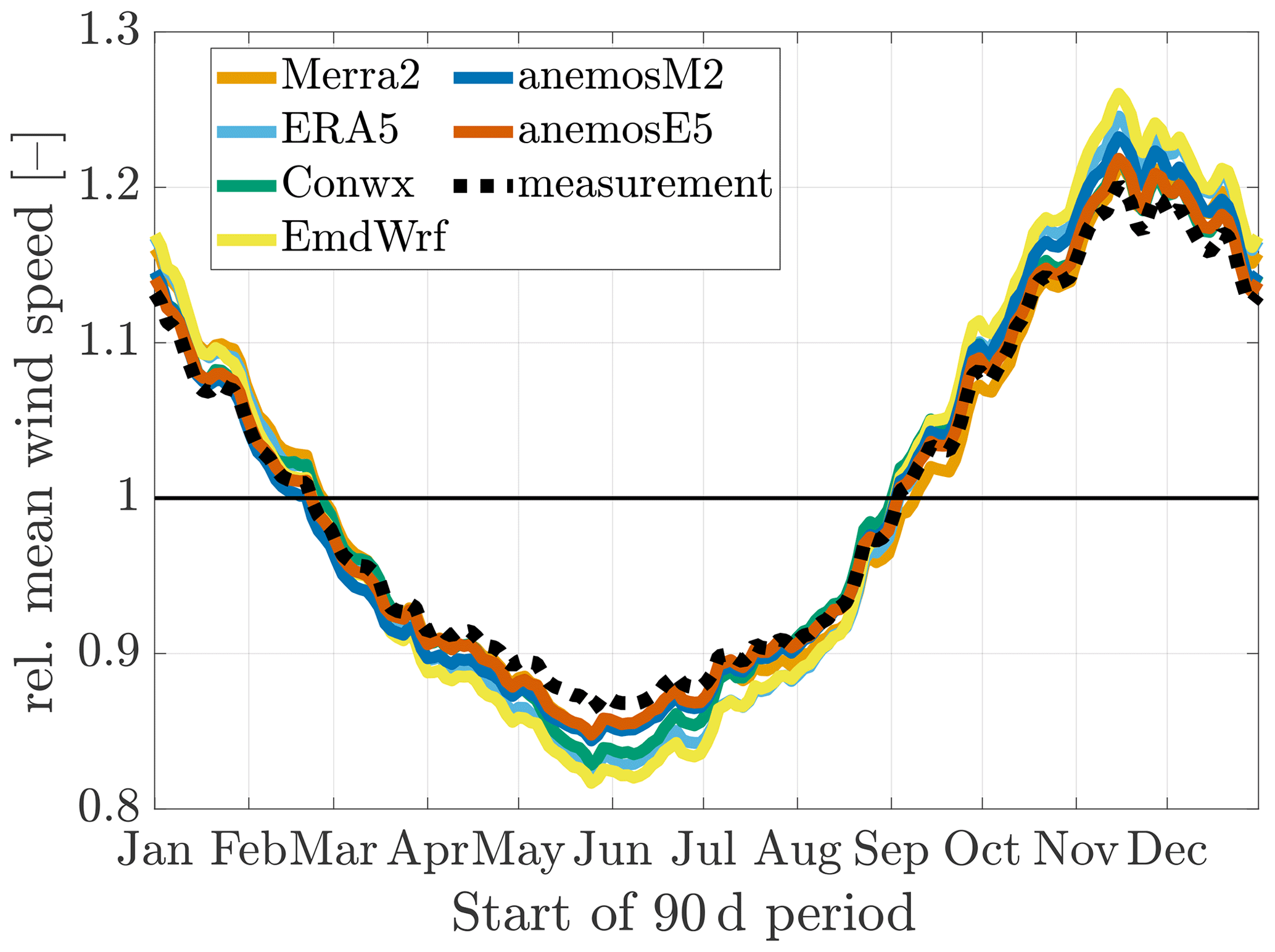
Figure 2 Average annual course of (normalized) wind speed in reanalysis and measurement data. Normalization was done by dividing the mean wind speeds observed in the 90 d periods by the respective annual mean. The individual results obtained at the 18 sites were then averaged arithmetically.

As the diagram shows, the annual course of wind conditions is marked by significantly lower mean wind speeds in summer and stronger winds in winter periods. This pattern typically prevails in Central Europe (Pryor et al., 2006). For all reanalysis data sets, however, the seasonal variations are overpronounced in comparison to the measured ones. In the transitional seasons (spring, fall), the deviations of (relative) reanalysis and measured wind speeds are smallest on average. The amplitudes of the curves in Fig. 2 differ, indicating clear differences between the reanalysis data sets.

In order to further analyze this aspect, a parameter d_mean was calculated aiming to display the deviations from reanalysis to measured data in the seasonal course. d_mean is derived based on mean values of reanalysis (${\stackrel{\mathrm{‾}}{u}}_{\mathrm{rea}}$) and measurement data (${\stackrel{\mathrm{‾}}{u}}_{\mathrm{meas}}$) during the 90 d periods in relation to their overall annual mean values (${\stackrel{\mathrm{‾}}{U}}_{\mathrm{rea}}$ and ${\stackrel{\mathrm{‾}}{U}}_{\mathrm{meas}}$, respectively):

$$\begin{array}{}\text{(16)}& d_{\mathrm{mean}}={\displaystyle \frac{{\stackrel{\mathrm{‾}}{u}}_{\mathrm{rea}}}{{\stackrel{\mathrm{‾}}{U}}_{\mathrm{rea}}}}-{\displaystyle \frac{{\stackrel{\mathrm{‾}}{u}}_{\mathrm{meas}}}{{\stackrel{\mathrm{‾}}{U}}_{\mathrm{meas}}}}.\end{array}$$

Hence, this quantity represents the difference between the colored lines and the measured seasonal course (black line) in Fig. 2. It therefore indicates the average error of the reanalysis data sets in reflecting the annual course of wind speed. According to the theoretical considerations in Sect. 4.2, this is an important aspect regarding the seasonal biases of an LTC (cf. term 1 and 2 in Eq. 13). For each short-term period, one value of d_mean per site and reanalysis data set is derived. Afterwards, values averaged over all sites are calculated, resulting in one set of d_mean values for each reanalysis data set.

Figure 3 shows the annual course of d_mean. Relatively large differences among the different reanalysis data sets can be observed. The overpronounced seasonal course of mean wind speed leads to negative values of d_mean in summer and positive values in winter periods for all reanalysis data sets. Comparing the global reanalysis data sets MERRA-2 and ERA5 shows advantages for the “older” MERRA-2 data set, as a lower amplitude in Fig. 3 is present. This holds true despite or because of the fact that the MERRA-2 data are provided at lower heights (50 m; see Sect. 2). This could generally be expected to yield a lower representativeness regarding the seasonal course at the measurement height. However, the ERA5-based anemosE5 data give better results than the MERRA-2-based anemosM2 data and, generally, show the highest accuracy regarding the seasonal course. This might be caused by the further developments by anemos when generating the anemosE5 model (e.g., the additional seasonal correction or the remodeling; see Sect. 2). The largest amplitude prevails for the EMD-WRF Europe+ data set.

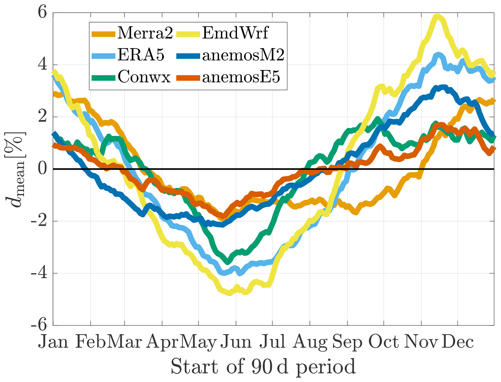
Figure 3 Deviation between reanalysis and measurement data in (normalized) mean wind speed (period of 90 d, arithmetically averaged over all sites).

5.2 Seasonal variations of regression parameter β₁ and correlation coefficient r_rea,meas

Motivated by their relevance in Eq. (13), average regression parameters β_1,VR and β_1,LR and their temporal variation during the year are investigated. These are shown in Fig. 4a and b. The respective values were calculated during 90 d periods and arithmetically averaged over all sites. Note that, as ${\mathit{\beta }}_{\mathrm{1},\mathrm{VR}}=\frac{{\mathit{\sigma }}_{\mathrm{meas}}}{{\mathit{\sigma }}_{\mathrm{rea}}}$ (see Eq. 7), Fig. 4a also gives an impression of how the reanalysis data reproduce the variance of wind speed and its temporal variation (Sect. 5.3 will address this aspect in more detail).

Figure 4 Temporal variations of regression parameter (a) β_1,VR for the variance ratio and (b) β_1,LR for the linear regression with residuals methods. The respective values were determined using a 90 d sliding window and arithmetically averaged over all sites.

Comparing the respective definitions of β₁ (Eqs. 2 and 7) shows that, for one pair of data sets, the LR method always produces smaller slopes than the VR method. In Fig. 4a and b this is clearly reflected. In contrast to β_1,VR, moreover, β_1,LR is subject to clear temporal variations showing lower values in summer and higher values in winter. This reflects the influence of the correlation coefficient r_rea,meas, which is part of the mathematical formulation of β_1,LR and which exhibits a seasonal pattern itself. This is depicted in Fig. 5, where normalized values of r_rea,meas are shown (similarly to the β₁ values in Fig. 4, these were averaged arithmetically over all sites). The correlation coefficient shows a clear seasonal variation for all reanalysis data sets and decreases significantly towards the summer periods. More unstable stratification and generally lower wind speeds (see Sect. 5.1) might be possible reasons.

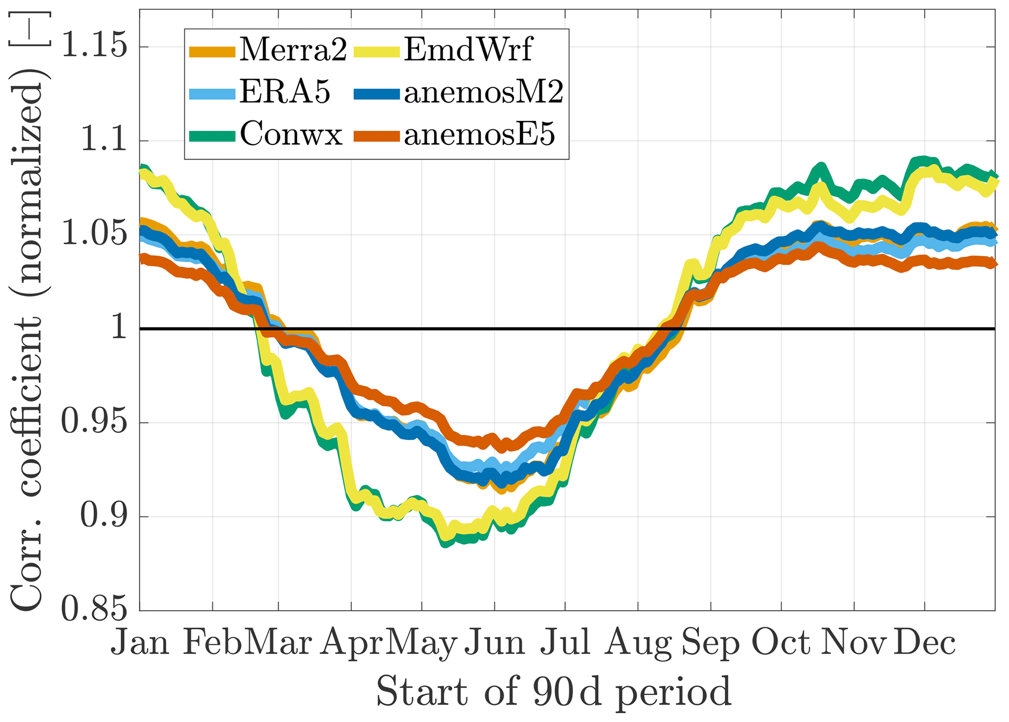
Figure 5 Normalized linear correlation coefficient between measurement and reanalysis data (periods of 90 d, arithmetically averaged over all sites). In the context of normalization the curves were shifted to a mean of 1 to better identify the (relative) temporal variations during the year.

According to Eq. (13), the respective β₁ value weights the seasonal course of the reanalysis data in the determination of the bias in mean wind speed. As a consequence of the findings here, the overpronounced seasonal cycle of the reanalysis data as depicted above is weighted more strongly in winter than in summer periods when the LR approach is applied. Moreover, lower weighting (in comparison to the VR method) occurs throughout as ${\mathit{\beta }}_{\mathrm{1},\mathrm{VR}}>{\mathit{\beta }}_{\mathrm{1},\mathrm{LR}}$.

5.3 Reproduction of the temporal variation of variance in the reanalysis data

In order to further investigate the capability of the reanalysis data in reproducing the seasonal course of variance, a measure d_var is calculated. Similarly to d_mean in Sect. 5.1, d_var is defined via the difference of relative values in the 90 d periods,

$$\begin{array}{}\text{(17)}& d_{\mathrm{var}}={\displaystyle \frac{\mathrm{Var}\left(u_{\mathrm{rea}}\right)}{\mathrm{Var}\left(U_{\mathrm{rea}}\right)}}-{\displaystyle \frac{\mathrm{Var}\left(u_{\mathrm{meas}}\right)}{\mathrm{Var}\left(U_{\mathrm{meas}}\right)}}.\end{array}$$

Figure 6 shows how the temporal variation of the measured variance throughout the year is reproduced by the different reanalysis data sets.

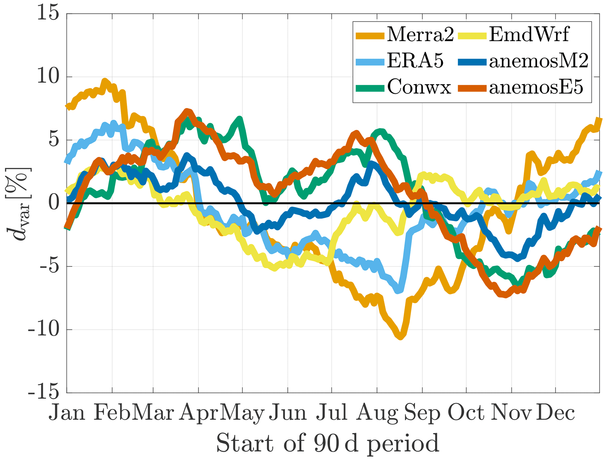
Figure 6 Deviation from reanalysis to measurement data in (normalized) variance (period of 90 d, arithmetically averaged over all sites).

The differences in variance reach values of up to ±10 % and are, therefore, generally higher than the deviations in mean wind speed (see Fig. 3). No universal seasonal dependence can be determined as it was observed for the mean wind speed. Some curves in Fig. 6 show minima in summer and high values in winter or spring, while others show contrary characteristics.

5.4 MCP calculations: seasonal bias in mean, variance, and energy

MCP calculations based on 90 d of measurement are now presented. For each reanalysis data set, an average value of the individual error scores related to one measurement period is calculated by arithmetically averaging over all sites. First, the focus of the analysis is put on mean and variance of wind speed. Afterwards, seasonal biases in the (theoretical) energy production of a wind turbine are analyzed. In this context, the influence of the systematic biases in both mean and variance on the accuracy in energy production is investigated on an experimental level. The analysis in these sections is focused on systematic biases first. The variability of the results (standard deviation) is presented and discussed in a dedicated section afterwards (Sect. 5.4.4).

5.4.1 Seasonal bias in mean wind speed

Figure 7a shows the experimentally obtained bias in mean wind speed (error score Err_mean) using the VR method. An inverse shape to the curves of d_mean (i.e., the error of the reanalysis data in the seasonal course; see Fig. 3) can be observed: a measurement in summer months results in a positive bias in the corrected wind speed time series, while a negative bias is produced when the measurement is conducted in winter. Thus, a positive bias is obtained when the reanalysis data underestimate the (relative) mean wind conditions which prevail in the measurement period and vice versa. These findings are valid for all reanalysis data sets, although it should be noted that the shapes of the related curves in d_mean are not transformed in the (inverse) course of Err_mean in exactly the same way.

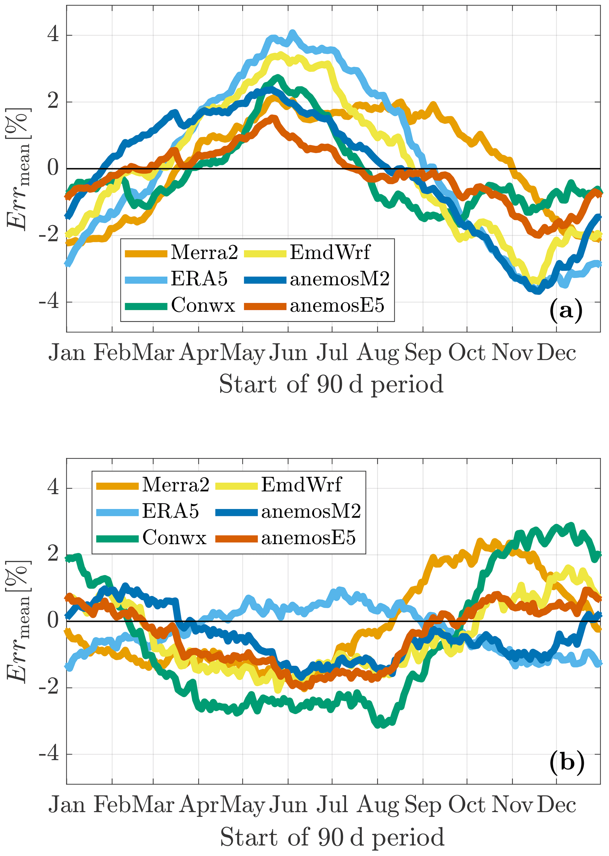
Figure 7 Temporal variations during the year of the bias in mean wind speed using the (a) variance ratio and (b) linear regression with residuals methods.

Strong differences compared to these observations and even contrary behavior can be found when the LR method is used (Fig. 7b). For all reanalysis data sets except ERA5, the mean of the corrected wind speed time series is underestimated in the case of measurements in summer, while overestimations prevail for winter measurements. The patterns seem not to be directly related to how the reanalysis data reproduce the measured seasonal course of the mean wind speed. Moreover, the ERA5 data give an inverse curve to all the other reanalysis data sets despite a high similarity in d_mean (Fig. 3). The amplitude of the respective curve is rather small, indicating only small seasonal biases. For most other data sets, the amplitudes of the curves in Fig. 7a and b are of comparable magnitude with a slight advantage for the LR method in predicting the mean of the corrected wind speed time series.

In line with the theoretical considerations in Sect. 4.2, the differences between Fig. 7a and b can be attributed to differences in β₁. As stated above, the VR method provides larger β₁ values than the LR approach. This leads to the fact that, generally, the seasonal course of the reanalysis data (term ${\stackrel{\mathrm{‾}}{u}}_{\mathrm{rea}}-{\stackrel{\mathrm{‾}}{U}}_{\mathrm{rea}}$ in Eq. 13) is weighted more strongly when the VR method is used. As a consequence, the effect of the overpronounced seasonal course of the reanalysis data, as presented in Sect. 5.1, dominates the result. This is underlined by the fact that Err_mean and d_mean roughly show inverse shapes (compare Fig. 7a with Fig. 3). For the LR approach, in contrast, the seasonal course of the reanalysis data is weighted less due to smaller β₁ values. Therefore, in most instances the seasonal pattern measured on-site (term ${\stackrel{\mathrm{‾}}{u}}_{\mathrm{meas}}-{\stackrel{\mathrm{‾}}{U}}_{\mathrm{meas}}$ in Eq. 13) dominates. Consequently, most curves of Err_mean show a high degree of similarity to the annual course of wind speed (Fig. 2).

As was shown in Fig. 4, in the case of the ERA5 data, relatively high β_1,LR values were obtained. For the LR method this causes a balancing effect (even slightly overbalanced). Thus, a relatively small amplitude of Err_mean can be observed in Fig. 7b despite, or rather because of, the overpronounced annual cycle of the ERA5 data. With regard to the VR method, again, the highest slopes (β_1,VR values) were observed for ERA5 compared to the other reanalysis data sets. As a direct consequence, the product of regression parameter β₁ and (overpronounced) seasonal course in the reanalysis data clearly dominates the result of Eq. (13), and the highest amplitude can be observed in Fig. 7a.

One further example is analyzed briefly here. The largest overestimation of the annual course of wind speed was found for the EMD-WRF Europe+ data set (see Fig. 3). In contrast to the ERA5 data, though, remarkably lower β_1,LR values are obtained when this reanalysis data set is used (see Fig. 4b). Eventually, the product of (small) regression parameter and (large) deviation of the reanalysis data in the seasonal course in Eq. (13) results in a relatively small amplitude of Err_mean.

In summary, it can be stated that the capability of the reanalysis data in reproducing the seasonal course of the true wind conditions on-site is an important aspect when considering the bias in mean wind speed. However, positive (or negative) deviations in the seasonal course do not transform to negative (or positive) biases directly. The regression parameter β₁, depending on both the MCP method and the selected reanalysis data set, strongly influences the outcome additionally.

Note that the influence of the seasonality in β_1,LR as shown in Fig. 4b can not be determined exactly here, as the lower values in summer coincide with a stronger effect of the overpronounced seasonal cycle of the reanalysis data (lower d_mean values).

In a study of Bass et al. (2000), long-term measurements instead of reanalyses were used as reference data. Long-term corrections of 1-year on-site data from Europe and the US were performed, testing a variety of MCP methods including linear models as well as a neural network approach. Regarding the bias in mean wind speed they found that none of the investigated methods stood out in comparison to the others. It was concluded that the success of the methods has “less to do with the mechanics of the methodology itself, and more to do with facets of the data being analysed”. Carta et al. (2013) confirmed that the uncertainty of long-term predictions depends much more on the (reference) data than on the MCP method.

With regard to an LTC of short-term wind measurements, the results of this work only partly agree with these findings from literature. It was shown both theoretically and experimentally that, concerning systematic, seasonal biases, a strong dependence on the selected MCP method occurs.

In a study of Weekes and Tomlin (2014a) seasonal patterns in the long-term correction of short-term wind measurements are addressed briefly. For both LR and VR, higher (more positive) values of the bias in mean wind speed were observed when measuring in summer, while smaller (more negative) values were obtained for winter measurements. The VR method yielded a smaller amplitude and, in contrast to the LR approach, resulted in negative biases throughout. Furthermore, it was concluded that the sign of the bias varied depending on the specific site when the VR method was applied. Weekes and Tomlin (2014a) related these seasonal effects to temporal changes in synoptic weather patterns and, connected to that, seasonal patterns in wind direction. No specific explanations were given for the differences between the results obtained with the VR or the LR method. It has to be noted that Weekes and Tomlin (2014a) used measurements instead of reanalysis data as reference, and all data were collected at heights of around 10 to 20 m. The theoretical background derived in Sect. 4.2, however, is valid independent of height and origin of the reference wind data. Against this background, it is likely that not all the reference data used in Weekes and Tomlin (2014a) exhibited an overpronounced seasonal cycle as is the case for the reanalysis data used in the study here.

Saarnak et al. (2014) applied a linear regression approach to wind data from a site on a Swedish island using MERRA reanalysis (predecessor of MERRA-2). Systematic underestimations in a long-term correction were found when short-term data of 3-month winter periods were used. Summer measurements, in turn, resulted in positive biases in mean wind speed. Hence, results similar to the ERA5 curve in Fig. 7 were obtained. Explanations for this seasonality were not given in the study.

In contrast to existing publications, therefore, this study delivers in-depth explanations of the seasonal biases and the differences when applying either the VR or the LR method for an LTC. The considerations in Sect. 4.2 provide the theoretical framework for this. In this context, it was shown that the biases are connected to properties of the reanalysis data set as well as characteristics of the MCP method.

5.4.2 Seasonal bias in variance

In this section, the bias of the MCP predictions with respect to variance is presented and discussed. Figure 8a and b show the respective error score Err_var.

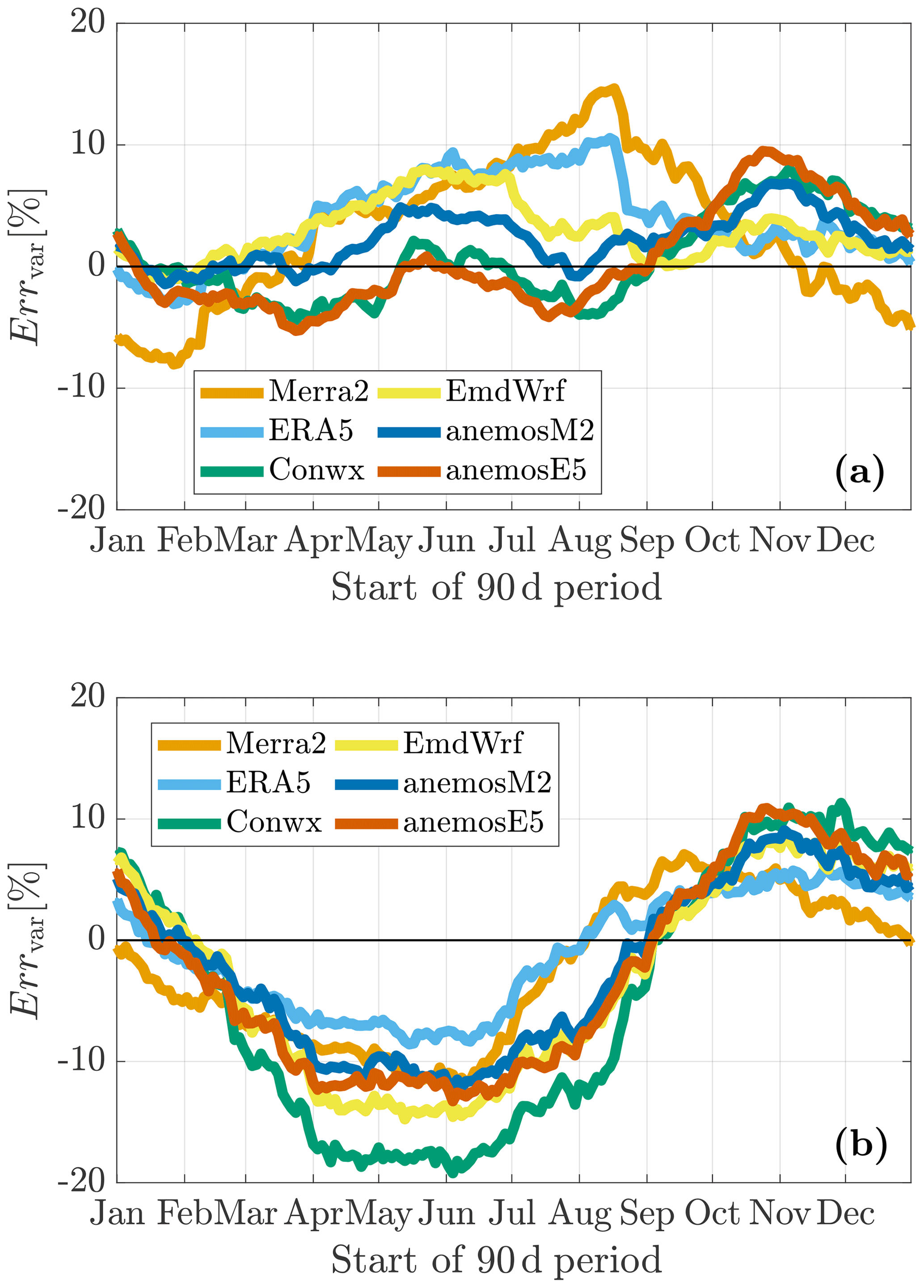
Figure 8 Temporal variations during the year of the bias in variance Err_var using the (a) variance ratio and (b) linear regression with residuals methods.

The curves displayed in Fig. 8a for the VR method resemble the inverse course of that observed in Fig. 6 and, thus, the patterns in the differences in variance of reanalysis and actually measured data. This is consistent with the theoretical considerations presented in Sect. 4.3 (in particular, see Eq. 14). Connected to that, no clear mean seasonal course can be observed when the VR method is used. The amplitudes of the variations, however, are of distinct magnitude, and remarkable errors can be observed.

As shown in Fig. 8b, there is a clear seasonal cycle of Err_var when applying the LR method. Lower values are found for measurements in summer, and higher values can be found for winter measurements. This effect can be observed for all reanalysis data sets. In Sect. 4.3 three parameters were identified which have a notable impact on Err_var when using the LR method. It is expected that the most important factor is the correlation coefficient r_rea,meas, since it contributes as a quadratic term to the theoretical calculation of Err_var (see Eq. 15). Moreover, this parameter exhibits a strong seasonal cycle similar to the course in Fig. 8b (see Sect. 5.2).

In summary, the amplitudes in Fig. 8b are generally of slightly larger magnitude than those of the variations produced by the VR method. This indicates that the VR method enables us to obtain a more accurate variance of the corrected data on average. Differences occur regarding the type of reanalysis data. Similar to the bias in mean wind speed, ERA5 gives the lowest bias in variance when the LR method is used, while large biases are obtained when the VR method is applied on the ERA5 data. In contrast to the mean wind speed, to the authors' knowledge the accuracy in variance has not been investigated in the literature.

5.4.3 Seasonal bias in the energy production of a wind turbine

In Sect. 4.1 a much greater importance of a high accuracy in mean than in variance was derived theoretically when aiming for a precise estimate of the energy in the wind. This contrasts with the finding of significantly higher biases in variance than in mean wind speed. In this section, the bias in the theoretical energy production of a wind turbine, Err_turbine, is discussed and compared to the other error scores. Going beyond the theoretical considerations on energy density in Sect. 4.1, this quantity involves the influence of the power curve and, therefore, reflects a practical measure for a central target value of wind resource assessment.

Err_turbine as obtained when using either the VR or the LR method is shown in Fig. 9. Comparison with the plots of Err_mean and Err_var (Figs. 7 and 8) reveals that the curves obtained here are very similar to those of the bias in mean wind speed (with about doubled amplitude). The influence of the bias in variance, in contrast, is barely visible. Only in specific periods when Err_var is large and its seasonal course does not follow the pattern of Err_mean, the influence of Err_var can be seen. This is most clearly visible in the case of the VR method (see, e.g., the data points related to the anemosE5 data in fall in Fig. 9a in comparison to Fig. 7a). It can be concluded that the biases in variance as depicted in Sect. 5.4.2 are even less relevant for the energy estimate of a wind turbine than the theoretical considerations in Sect. 4.1 suggest. One explanatory aspect here may be that variations of very large wind speed values (exceeding the rated wind speed of the turbine) contribute strongly to variance but have no influence on the energy output.

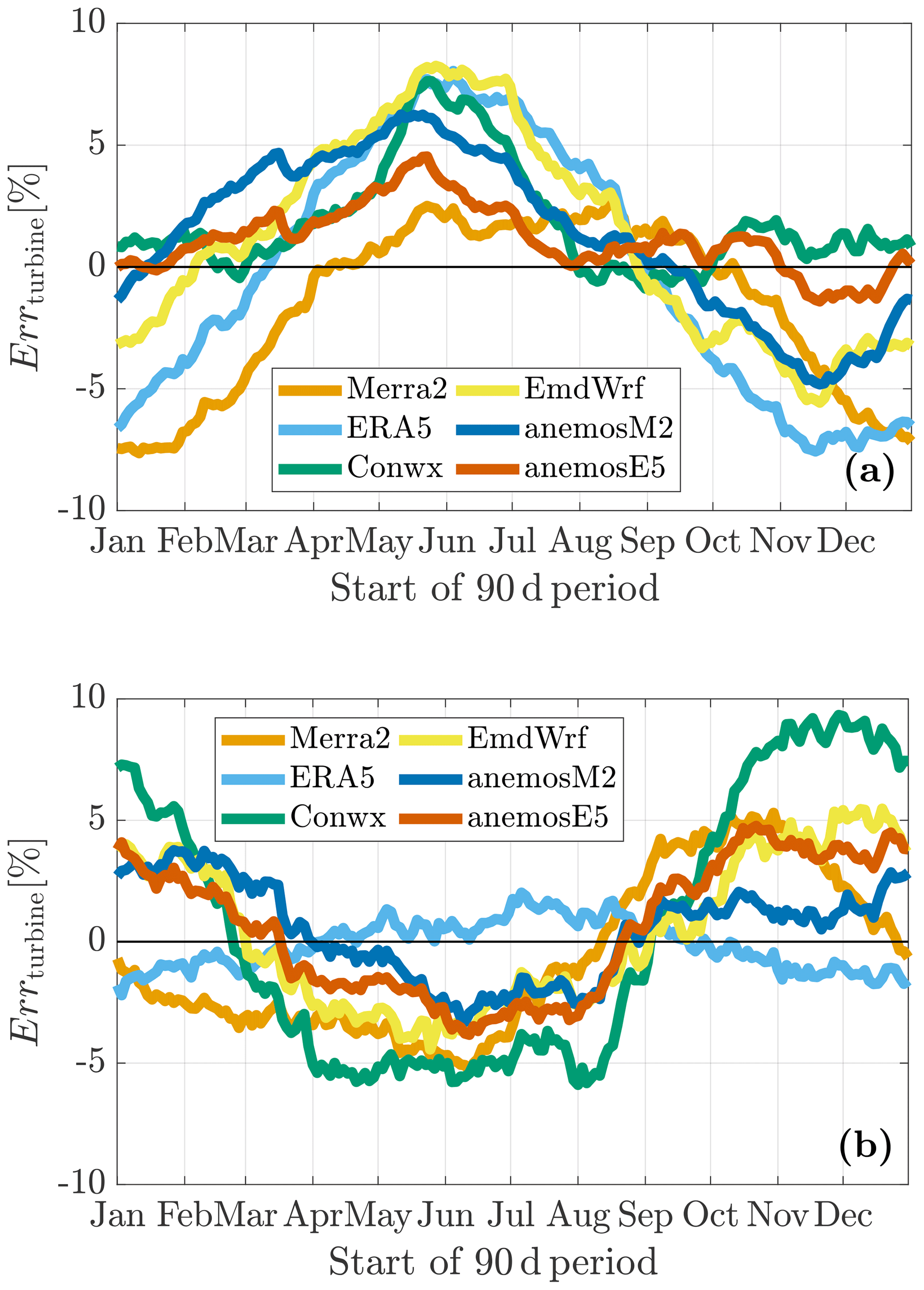
Figure 9 Temporal variations during the year of the bias in the theoretical annual energy production of a wind turbine Err_turbine using the (a) variance ratio and (b) linear regression with residuals methods.

Besides that, one specific characteristic of Err_turbine stands out when the VR method is applied (Fig. 9a): some curves mostly lie above or below zero for the entire year. Such overall biases are present especially in the case of the EMD-ConWx (positive overall bias) and the MERRA-2 data (negative overall bias). When applying the LR method (Fig. 9b), hardly any overall bias can be found.

Towards an explanation approach for this observation, the regression parameters β₀ (offset) and β₁ (slope) have to be considered. For the VR method, higher β₁ values and, due to the relationship of β₁ and β₀ in Eq. (3), lower β₀ values are obtained compared to the LR approach. This is visualized in the scatter plot in Fig. 10 where distinct differences between the regression lines can be observed. As a consequence, smaller wind speed values are generally corrected towards smaller values, while higher values are increased compared to the correction applied in the LR method. Similar correction is performed for wind speeds near the mean (i.e., values close to 1 in Fig. 10).

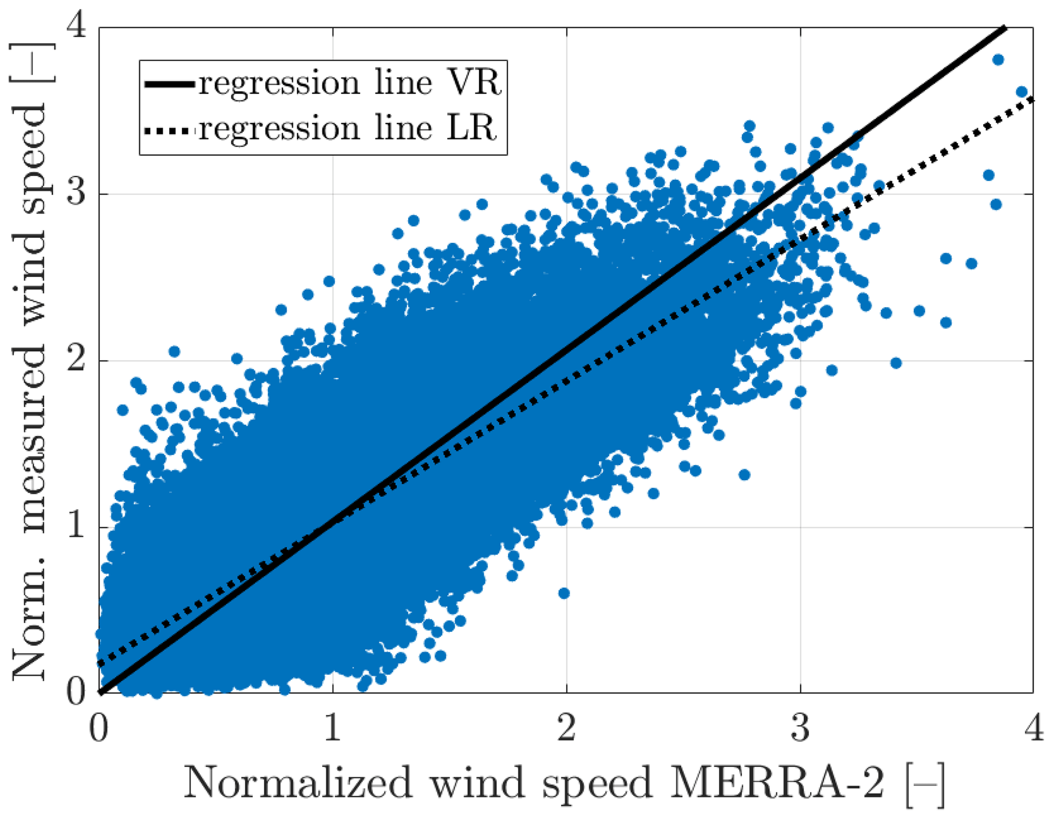
Figure 10 Scatter plot of normalized measured and MERRA-2 data and regression lines to these data using either the VR or the LR method. Normalization was performed by dividing all wind speed values by the overall measured mean. The diagram was produced using the entire measurement data of the 18 sites (at the heights specified in Table 1) and the related MERRA-2 data (see Sect. 2).

This aspect can be expected to average out when considering mean wind speeds. However, it apparently becomes important in the case of energy production estimation where the shape of the power curve leads to a different importance (or weighting) of wind speed values of different ranges. Any wind-speed-dependent errors of the reanalysis data can further contribute to this issue.

5.4.4 Variations between the sites

The variations between the sites can be judged an important measure to characterize the reliability of the results. Furthermore, they give an indication for the uncertainty if the systematic, seasonal biases could be removed (e.g., by applying a correction function). Therefore, the standard deviations of Err_mean and Err_turbine in dependence of the measurement period are addressed here and shown in Fig. 11. The analysis is restricted to these error scores as they are expected to be most useful for the wind industry.

Figure 11 Bias variations between the sites (1 SD – standard deviation) with regard to the accuracy of predicting the mean wind speed (a, b) and the theoretical energy production of a wind turbine (c, d). The panels on the left (a, c) refer to the VR method, while in panels (b) and (d) the results produced by the LR method are shown.

Similar to the biases, the variations (standard deviations) are significantly higher for Err_turbine than for Err_mean. In general, both methods (VR and LR) produce comparable magnitudes, while the results, again, strongly depend on the selected reanalysis data. The maximum values for individual reanalysis data sets in Fig. 11 are lowest for the anemos data sets and range from approximately 1 % to 5 % in the case of Err_mean. Differences regarding the MCP method occur in winter periods when considering Err_turbine (9 % in maximum values for the VR method and more than 11 % for the LR method). In summary, the variation between the sites is roughly of the same magnitude as the bias values themselves (see Fig. 9).

On average, smallest values can be observed in the beginning of the year and in fall (i.e., measurement periods starting in January/February or September/October) for both Err_mean and Err_turbine. This indicates that not only strong biases are present when the measurement is conducted in summer or winter but also higher variations and, hence, smaller reliability of these biases can be expected. Moreover, this underlines the significance and importance of a sorrow selection of the measurement period, with transitional seasons (spring, fall) to be recommended in Central Europe.

6 Conclusions and outlook

This study delivered in-depth analysis of seasonal effects in the long-term correction of short-term wind measurements. The provided findings can contribute to a further development of reanalysis data as well as improved MCP methods in this respect.

In a first step, the importance of the accuracy in mean and variance of wind speed was evaluated with regard to a precise estimate of the energy in the wind. It was shown on a theoretical level that the relative error in mean contributes 6 times as much as the relative error in variance in this context. Experimental analysis, in contrast, showed that much larger biases in variance than in mean prevail when MCP predictions are performed (absolute values of more than 15 % were obtained in comparison to values of ±4 %, respectively). It was demonstrated that – apart from overall biases – the shape of the seasonal course of the bias in mean wind speed was more or less replicated in the bias of the theoretical energy production. Therefore, it can be concluded that a precise estimate of the mean is much more important than the correct estimate of the variance when assessing the energy production of a wind turbine.

A formula was derived which delivered the explanation for the seasonal biases in mean wind speed when applying either the variance ratio or linear regression with residuals method. It was shown that the representativeness of the measurement period, i.e., the similarity of the wind conditions in correlation and correction period, is important. Moreover, the capability of the reference (here reanalysis) data to reproduce the seasonal course proved to be a decisive factor. Lastly, the regression parameter β₁ (computed differently for the two MCP methods used in this study) was shown to influence the magnitude of the seasonal biases significantly. With this theoretical framework, it was possible for the first time to attribute errors in the long-term correction to characteristics of the MCP method as well as properties of the reanalysis data set.

The largest biases were obtained in the case of measurement periods with non-representative wind conditions (i.e., significantly lower or higher mean wind speeds compared to the annual mean – usually summer and winter periods in Central Europe). The magnitude was shown to depend on the reanalysis data set. Furthermore, a strong dependence on the MCP method was identified; very different, partly even contrary characteristics in the seasonal biases were found for the VR and LR methods.

In general, measurement periods in transitional seasons (spring, fall) not only resulted in smallest biases but also gave the smallest variation between the sites and, thus, the highest reliability of the results. The amplitudes of seasonal bias and standard deviation of the results obtained at the individual sites were roughly of the same magnitude. If short-term wind measurements are used for wind resource assessments, it is, therefore, highly recommended to conduct these measurements in periods which are likely to be characterized by representative wind conditions (with respect to mean wind speed).

Further research is necessary on how the systematic biases and, finally, the uncertainty of the long-term correction of short-term wind measurements can be reduced in an efficient and expedient way. The authors suggest that this could be approached in different ways. On the one hand, a manual correction based on the experiences described above would reduce the biases. However, the reliability (standard deviation) would not change. A statistics-based approach (e.g., averaging the results of different MCP approaches and/or reference data) as well as machine learning approaches (e.g., learning the seasonal effects from other data sets) might result in larger improvements. On the other hand, the shortcomings of the reference (here reanalysis) data in reproducing the seasonal course could be addressed. Discrepancies regarding temporal changes in synoptic weather patterns or atmospheric stability processes can be named as possible examples for such weaknesses. The inclusion of further meteorological data reflecting these characteristics could form the basis of a physically motivated approach here. The usefulness of removing seasonal biases in, e.g., wind profile extrapolation by including additional parameters like relative humidity was demonstrated in Basse et al. (2020). This approach could also be taken here.