The 3 km Norwegian reanalysis (NORA3) – a validation of offshore wind resources in the North Sea and the Norwegian Sea

We validate a new high-resolution (3 km) numerical mesoscale weather simulation for offshore wind power purposes for the time period 2004–2016 for the North Sea and the Norwegian Sea. The 3 km Norwegian reanalysis (NORA3) is a dynamically downscaled data set, forced with state-of-the-art atmospheric reanalysis as boundary conditions. We conduct an in-depth validation of the simulated wind climatology towards the observed wind climatology to determine whether NORA3 can serve as a wind resource data set in the planning phase of future offshore wind power installations. We place special emphasis on evaluating offshore wind-power-related metrics and the impact of simulated wind speed deviations on the estimated wind power and the related variability. We conclude that the NORA3 data are well suited for wind power estimates but give slightly conservative estimates of the offshore wind metrics. In other words, wind speeds in NORA3 are typically 5 % (0.5 m s⁻¹) lower than observed wind speeds, giving an underestimation of offshore wind power of 10 %–20 % (equivalent to an underestimation of 3 percentage points in the capacity factor) for a selected turbine type and hub height. The model is biased towards lower wind power estimates due to overestimation of the wind speed events below typical wind speed limits of rated wind power (u<11–13 m s⁻¹) and underestimation of high-wind-speed events (u>11–13 m s⁻¹). The hourly wind speed and wind power variability are slightly underestimated in NORA3. However, the number of hours with zero power production caused by the wind conditions (around 12 % of the time) is well captured, while the duration of each of these events is slightly overestimated, leading to 25-year return values for zero-power duration being too high for the majority of the sites. The model performs well in capturing spatial co-variability in hourly wind power production, with only small deviations in the spatial correlation coefficients among the sites. We estimate the observation-based decorrelation length to be 425.3 km, whereas the model-based length is 19 % longer.

1 Introduction

Exploiting the Norwegian continental shelf for offshore wind power purposes is advantageous due to the excellent wind climate (Zheng et al., 2016) and the recent increase in political engagement. In June 2020 the Norwegian government decided to open the country's first two offshore areas at the Norwegian continental shelf, “Utsira Nord” and “Sørlige Nordsjøen II”, for concessions to build and operate large wind power installations (Regjeringen, 2020). In this context, the ability to map the spatial and temporal wind power potential is crucial for selecting the best areas for wind power production.

Observational sites in the North Sea and the Norwegian Sea are sparse, and their numbers are insufficient to map the regional wind power potential. The lack of observational data makes it challenging for stakeholders and decision makers to choose new sites to open for offshore wind power concessions. Apart from using satellite data on surface winds, the only way to map the total wind power potential for a large offshore area is to use data from high-resolution numerical weather prediction (NWP) models that provide data near a typical hub height.

Several studies have mapped the wind energy potential of the North Sea and/or the Norwegian Sea using simulated data from the mesoscale Weather Research and Forecasting (WRF) Model (Berge et al., 2009; Byrkjedal and Åkervik, 2009; Byrkjedal et al., 2010; Skeie et al., 2012; Hahmann et al., 2015; Hasager et al., 2020). Berge et al. (2009) investigated how well the WRF model captured the offshore wind conditions in the North Sea from 2004–2007. After comparison of the simulated data with observations from oil and gas platforms, the authors conclude that the WRF model is a reliable tool for characterizing the average wind conditions in the region in question. The model was verified using observations from offshore sites in the North Sea but did not undergo a peer-review process. Byrkjedal and Åkervik (2009) simulated the wind resource and wind power potential at the Norwegian economic zone. The WRF model produced the simulated data for 2000–2008 used in their wind power calculations. However, the simulated data set was not validated against observations, and the report was not peer-reviewed. Byrkjedal et al. (2010) used the WRF model to simulate the offshore wind power potential in the North Sea from 2000 to 2009. Based on their 10-year WRF simulation they estimated wind power and identified areas with the greatest wind power potential, in addition to the dependency between separation distance and the correlation between two wind power production sites. The model performance was not compared to observations, and the report was not evaluated in a peer-review process. The more recent data set, the New European Wind Atlas (NEWA), was a joint project between research institutions and the industry. NEWA aims to provide a high-resolution, freely available data set on wind energy resources in Europe (Dörenkämper et al., 2020). NEWA uses meteorological masts on land to validate the onshore model data, while the offshore data are validated at 10 m a.s.l. (meters above sea level) using satellite data. In addition, a validation at 100 m a.s.l. is conducted by extrapolating the equivalent neutral wind speed at 10 m using the log-law relation (Badger et al., 2016). NEWA underwent a peer-review process. A peer-reviewed validation of wind model simulations before using the data for offshore wind power purposes is very important. The degree of data set validation and peer-review process of the results in the preceding studies is either limited or nonexistent.

In this study we perform an in-detail validation of the 3 km Norwegian reanalysis (NORA3), a new and freely available high-resolution data set, to be used for offshore wind resource assessment and wind power estimates. NORA3 is a high-resolution atmospheric dynamic downscaling of the state-of-the-art reanalysis data from ECMWF, called ERA5. The downscaling of ERA5 is performed by the NWP model HARMONIE-AROME (H-A). H-A is a high-resolution NWP model developed and used by many European weather forecast and research institutions (Seity et al., 2011; Bengtsson et al., 2017). The creation of NORA3 will contribute to the growing ensemble of wind resource data sets. Since all currently existing wind resource data sets are generated by the WRF model, the creation of NORA3 by a different NWP model will contribute to a diversity in the available wind resource data sets. When the ensemble of these data sets is considered in wind power planning the overall uncertainty in power production can be better quantified. The usefulness of multi-model ensembles has become increasingly clear over the last few decades in research fields such as weather prediction and climate change. By this extensive validation of the NORA3 data set and documenting the quality of the simulated wind resource and related wind power estimates from a new model, we wish to contribute to the growing literature on offshore wind resources.

The novelty of this study is the in-depth validation of the model data using a new NWP model. Through advanced statistical measures we perform a near-hub-height validation of the NORA3 estimated wind resource and the related wind power production. Besides validation measures like arithmetic mean, standard deviation, relative difference between the data sets, temporal correlations, and seasonality of the variables, we also include comparison and validation of data distributions, hourly ramp rates, spatial correlation, and analysis on the zero-wind-power events including extreme-value analysis. Since this is the first paper to evaluate the wind resource estimates from NORA3, the focus is put on a detailed validation against observations. A comparison of NORA3 against the host data set (ERA5) is also conducted to document the improvement of the downscaling process. To our knowledge this is the first peer-review paper focusing on evaluation of simulated wind resource and wind power estimates against offshore observations in the North Sea and adjacent ocean regions, increasing the relevance of the present study.

We validate the NORA3 data set for wind power purposes using observational wind data from six offshore sites. Details regarding the model and observational data, in addition to the data processing routines, are found in Sect. 2.1 and 2.2. Sections 2.3–2.6 describe the methods used. The result of the downscaling process of ERA5 is quantified through a comparison between output data from NORA3 and ERA5 in Sect. 3. In Sect. 4 we investigate how well NORA3 captures the statistical wind speed measures and the related distributions. We also study the model performance in terms of the wind speed ramp rates (Sect. 4.1), spatial wind speed gradient (Sect. 4.2), and wind direction (Sect. 4.3). In addition, uncertainties related to observations sampled at large structures are discussed in Sect. 4.4. After converting wind speed data to hourly wind power data, we examine the performance of NORA3 related to wind power climatology (Sect. 5), including wind power variables such as median production and capacity factor (CF). Revealing the wind power potential in an area also requires mapping the wind power intermittency and variability at different spatial and temporal scales. The ability of the model to capture wind power variability and intermittency is investigated using hourly wind power ramp rates (Sect. 5.1) and long-term variability in CF (Sect. 5.2). In addition to temporal variability, we also consider the ability of NORA3 to capture the spatial co-variability between production sites (Sect. 5.3). It is crucial for a data set to reveal the length, duration, and total number of hours of zero wind power production, and NORA3's performance against these measures is discussed in Sect. 5.4. Moreover, we calculate and validate the maximum expected length of a zero event occurring during the turbine lifetime (Sect. 5.5). In the last section (Sect. 6) we summarize the validation results.

2 Data and method

2.1 Model data

NORA3 is obtained by high-resolution atmospheric dynamic downscaling of the state-of-the-art ERA5 reanalysis data set from the ECMWF (Hersbach et al., 2020). ERA5 covers the Earth in an approximately 31×31 km horizontal grid, providing hourly information in 137 vertical layers. The model used in the downscaling process is the nonhydrostatic, convection-permitting NWP model HARMONIE-AROME (H-A) (Cycle 40h1.2). Boundary values from ERA5 are provided to the model every 6 h. Hourly¹ NORA3 output data are stored (some outputs are stored every third hour). The model domain in NORA3 encloses almost the entire northern part of the Atlantic Ocean (see Fig. 1), and the model runs with a horizontal resolution of 3×3 km, with the atmosphere divided into 65 vertical layers.

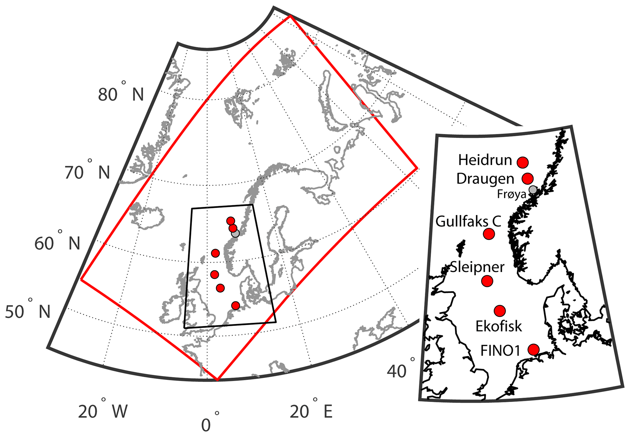
Figure 1 The domain (red rectangle) covered by the HARMONIE-AROME simulation and the locations of the six sites used in verifying the NORA3 data set (red dots), in addition to the meteorological mast located at Frøya. A close-up plot of the positions and the names of the stations is also shown. Details for the sites are given in Table 1.

H-A is a high-resolution NWP model solving the fully compressible Euler equations using forward time integration on a non-staggered horizontal grid. H-A is used in short-range operational forecasting and research by many European weather services and research institutes (Seity et al., 2011; Bengtsson et al., 2017). The NORA3 data set is a hybrid between a hindcast and a reanalysis data set because of the way the observations are treated in the model. The H-A model performs data assimilation of 2 m temperature and 2 m relative humidity.

NORA3 is continuously being generated. When the model integration is finalized (summer 2022) the NORA3 data will cover the time period from 1979 to present and will be regularly updated in the coming years when ERA5 data become available. We will focus on the period 2004–2016 in this study due to the time coverage of the observational data. For further details on the model set-up and the NORA3 generation process see Haakenstad et al. (2021).

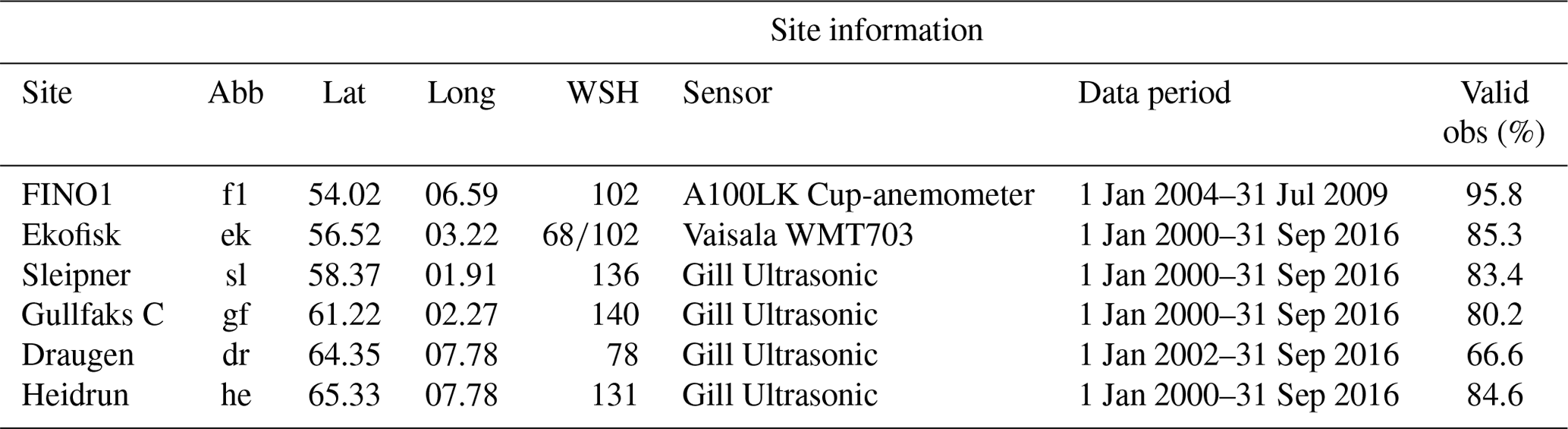
Table 1 Relevant information for the sites used in the validation of NORA3. “Abb” lists the site-name abbreviations. “Lat” and “Long” are the latitude and longitude for the site locations, respectively. “WSH” (in meters above sea level) corresponds to the wind sensor height at each site. The sensor type is listed under “Sensor”, and the data period for the available observations for each site is listed under “Data period”. In addition, the percentage of valid observations is also shown under “Valid obs (%)”.

2.2 The observational data

The observations used in the verification of NORA3 are hourly wind observations² from five oil and gas platforms (Ekofisk, Sleipner, Gullfaks C, Draugen, and Heidrun) retrieved from the Norwegian Meteorological Institute and one meteorological mast (FINO1, mast corrected data) (see Fig. 1 for the location of the sites and Table 1 for further site information). The observational data were quality checked prior to the validation of NORA3. For a detailed description of this quality check process see Solbrekke et al. (2020). In addition to the routine described in Solbrekke et al. (2020), we also exclude all records of zero-wind conditions (u=0) that are likely to be erroneous according to the following:

$$\begin{array}{}\text{(1)}& \begin{array}{rl}{u}_{\mathrm{obs}}\left(i\right)& =\mathrm{0}\bigwedge u_{\mathrm{n}\mathrm{3}}\left(i\right)\ge {\displaystyle \frac{\mathrm{5}}{m}}{\displaystyle \frac{\mathrm{1}}{n}}\sum _{j=\mathrm{1}}^m\sum _{i=\mathrm{1}}^n\left|u_{\mathrm{obs}}\right(i,j)-u_{\mathrm{n}\mathrm{3}}(i,j\left)\right|\\ & =\mathrm{5}\stackrel{\mathrm{‾}}{\mathrm{MAD}},\end{array}\end{array}$$

where u_obs(i,j) and u_n3(i,j) are the observed and modeled wind speeds, respectively, at hour i for site j. n is the total number of hours, m is the total number of sites, and $\stackrel{\mathrm{‾}}{\mathrm{MAD}}$ is the mean absolute deviation between the observed and modeled wind speeds averaged over all sites. In other words, whenever the observed wind speed at hour i and site j is zero and the corresponding modeled wind speed exceeds $\mathrm{5}\stackrel{\mathrm{‾}}{\mathrm{MAD}}=\mathrm{7.2}$ m s⁻¹, the observed value at hour i is excluded from the time series for site j. This additional quality control leads to the exclusion of up to 5 h of observations per site, except at Heidrun, which excludes 58 h of observations. For Heidrun, the removal of these erroneous records of zero-wind conditions (u=0) corresponds to an exclusion of approximately 0.035 % of the total data.

2.3 Wind interpolation

To avoid introducing additional uncertainties into the observational data set, we verify the wind variables from NORA3 at the wind sensor heights, ranging from 68–140 m a.s.l., for each site (see “WSH” in Table 1 for the sensor heights). By contrast, the wind power verification is performed at a typical hub height, at 100 m a.s.l., to ensure the production estimates are comparable between sites. The interpolation of wind speed data to another height is usually done by either the logarithmic law, the power law, or a combination of the two methods (e.g., the Deaves & Harris model). Gualtieri (2019) reviewed the three aforementioned methods for 96 different locations worldwide. He concluded that the power law was the most reliable and also the most frequently used extrapolation method. In addition, according to Sill (1988) the usage of the logarithmic law (log law) is most suitable near the surface. Despite the aforementioned results from Gualtieri and Sill we have compared the performance of the log law and the power law (with time varying power exponent) for the offshore sites. The results of the comparison show that the model bias using the log law is larger than using the power law method. Therefore, the interpolation of wind speed data to sensor height or hub height is done using the power law relation (Emeis, 2018).

The interpolated wind speed is sensitive to the choice of the power law exponent α. Usually, α is assigned based on assumptions about atmospheric stability and surface roughness, both of which can introduce erroneous results. However, the data from NORA3 allow us to calculate α for each time step (i). Rearranging the power law relation, we get the following expression for the power law exponent α:

$$\begin{array}{}\text{(2)}& \mathit{\alpha }\left(i\right)={\displaystyle \frac{\ln \frac{u(i{)}_{z\mathrm{2}}}{u(i{)}_{z\mathrm{1}}}}{\ln \frac{z_{\mathrm{2}}}{z_{\mathrm{1}}}}},\end{array}$$

where the height subscripts ₁ and ₂ corresponds to the two layers within which the wind shear is calculated. The heights used to calculate α depend on the wind sensor height (WSH) at the site in question: if WSH < 100 m a.s.l. then α is calculated using NORA3 wind shear between the two model layers z₁=50 m a.s.l. and z₂=100 m a.s.l. If WSH > 100 m a.s.l., then α is calculated using the wind shear between z₁=100 m a.s.l. and z₂=250 m a.s.l. The mean α for the whole time period for the six stations ranges from 0.05 to 0.08 between 50 and 100 m a.s.l. and from 0.03 to 0.06 between 100 and 250 m a.s.l. For each site, the wind directions at WSH are obtained by interpolating the X and Y component of the wind vector using linear interpolation between the adjacent model layers (50 and 100 m a.s.l. or 100 and 250 m a.s.l.).

2.4 Normalized wind power

To ensure our validation results are as general as possible, and since the wind farm at each site is only imaginary and of unknown capacity, we use normalized power calculations $P_{\mathrm{w}}\left(i\right)=\frac{P_w^T\left(i\right)}{P_{\mathrm{w}}^{\max }}$ to validate the wind power potential at each site (Solbrekke et al., 2020). $P_{\mathrm{w}}^T\left(i\right)$ is the produced wind power at each time step (i) for a given site, and $P_{\mathrm{w}}^{\max }$ is the nameplate capacity. Hence, the normalized wind power P_w(i) is defined as follows:

$$\begin{array}{}\text{(3)}& P_{\mathrm{w}}\left(i\right)=\left\{\begin{array}{ll}\mathrm{0}& u\left(i\right)<u_{\mathrm{ci}},\\ \frac{u(i{)}^{\mathrm{3}}-u_{\mathrm{ci}}^{\mathrm{3}}}{u_r^{\mathrm{3}}-u_{\mathrm{ci}}^{\mathrm{3}}},& u_{\mathrm{ci}}\le u\left(i\right)<u_r,\\ \mathrm{1},& u_r\le u\left(i\right)<u_{\mathrm{co}},\\ \mathrm{0},& u_{\mathrm{co}}\le u\left(i\right),\end{array}\right.\end{array}$$

where u(i) is the wind speed at hour i, u_ci=4 m s⁻¹ is the cut-in wind speed, u_r=13 m s⁻¹ is the rated wind speed, and u_co=25 m s⁻¹ is the cut-out wind speed. These numbers were retrieved from the SWT-6.0-154 turbines used in Hywind Scotland – the first floating wind farm in the world (Siemens Gamesa Renewable Energy, 2011).

2.5 Ramp rates

To validate the ability of NORA3 to capture the wind speed and wind power variability, we calculate the ramp rates (R), defined as how much the wind speed (u) or wind power (P_w) changes during a time increment τ (Milan et al., 2014):

$$\begin{array}{}\text{(4a)}& {\displaystyle }& {\displaystyle }{R}_{{\mathrm{P}}_{\mathrm{w}}}\left(i\right)=P_{\mathrm{w}}\left(i\right)-P_{\mathrm{w}}(i+\mathit{\tau }),\text{(4b)}& {\displaystyle }& {\displaystyle }{R}_u\left(i\right)=u\left(i\right)-u(i+\mathit{\tau }),\end{array}$$

and setting τ=1, we validate the model performance on hourly ramp rates. To gain a general picture of the model performance in terms of how much the wind speed or wind power changes from one hour to the next, we calculate the mean absolute ramp rate (MAR) for each site, for both the observational data and the modeled data. MAR is defined as follows:

$$\begin{array}{}\text{(5)}& \mathrm{MAR}={\displaystyle \frac{\mathrm{1}}{n}}\sum _{i=\mathrm{1}}^n\left|R\right(i\left)\right|,\end{array}$$

where R(i) is the ramp rate at hour i and n is the total number of hours.

2.6 Zero-event duration using extreme-value theory

A wind turbine has an expected lifetime of approximately 20 years. If the right steps are taken, the lifetime can be extended 15 %–25 % depending on whether the structure is bottom-fixed or floating (Wiser et al., 2016). This means that the lifetime is expected to increase to 23–25 years. Therefore, determining the duration of long-lasting shutdowns expected to happen during the lifetime of a turbine is important for estimating the levelized cost of energy (LCOE). The 25-year return value of the duration of a zero event (a period of zero wind power production), the corresponding confidence interval, and the p values are calculated from the observations and the model data using two statistical methods, “block maxima” (BM), in which the data are fitted to a generalized extreme value (GEV) distribution using yearly values of maximum zero-event duration, and “peak over threshold” (POT), in which the data are fitted to a generalized Pareto distribution (for more information see Smith, 2002) using the 99th percentile of the zero-event duration (the highest 1 % of zero event in terms of duration) as the selected threshold. We calculate the Kolmogorov–Smirnov p value (KS_p) to test the null hypothesis. The null hypothesis states that the empirical data are not drawn from the chosen data distribution (GEV or Pareto). Testing the null hypothesis is done by the Kolmogorov–Smirnov statistic calculating the distance between the empirical and theoretical cumulative distributions. Hence, the cumulative distribution function from the BM data (POT data) is compared to the cumulative distribution function from the GEV (Pareto) distribution. Thus, given a significance level of p=0.025, if the KS_p value is small (KS_p<p), the distance between the cumulative distributions is too large, and we can conclude that the empirical data (BM or POT) was sampled from a different population than the theoretical GEV or Pareto distribution with a probability of 1−p. If the result from the Kolmogorov–Smirnov test tell us that we cannot exclude the possibility that the data are drawn from either of the two data distributions (GEV or Pareto), we fit the observation-based and model-based maximum zero-event durations to GEV and Pareto and find the corresponding 25-year return values for the five sites (FINO1 is excluded from the extreme-value analysis due to the shorter time series: 2004–2009).

Table 2 Seasonal average of the observed (obs) wind speed (m s⁻¹) and the model deviation in percentage (%) for both NORA3 (n3) and ERA5 (e5). “DJF” corresponds to December–January–February, “MAM” is March–April–May, “JJA” is June–July–August, and “SON” is September–October–November.

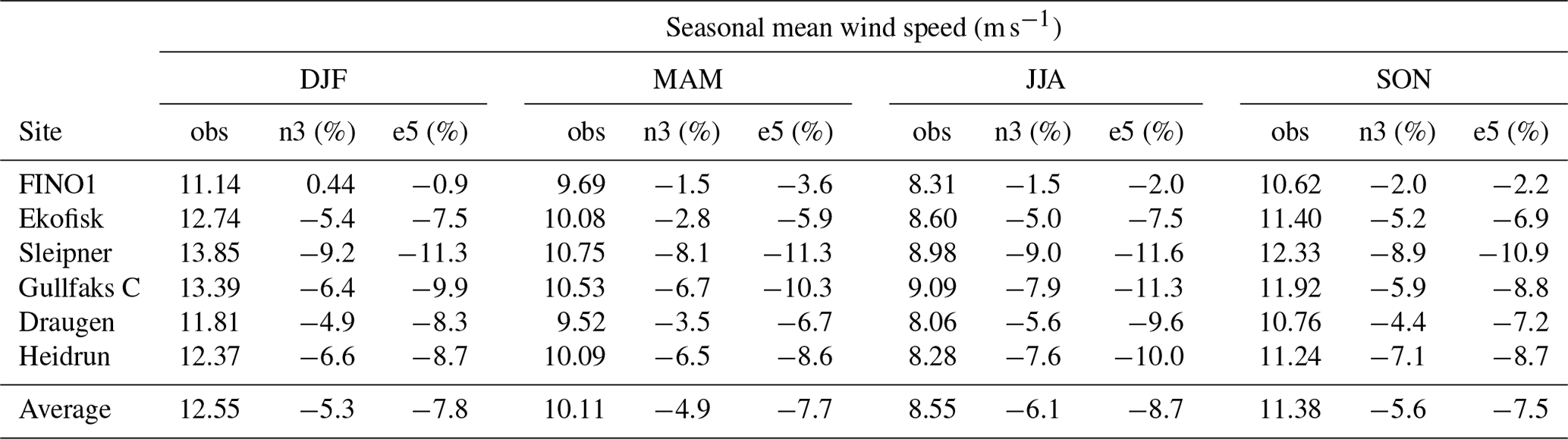
Table 3 Seasonal standard deviation of the observed (obs) wind speed (m s⁻¹) and the model deviation in percentage (%) for both NORA3 (n3) and ERA5 (e5). “DJF” corresponds to December–January–February, “MAM” is March–April–May, “JJA” is June–July–August, and “SON” is September–October–November.

3 Comparison of NORA3 and ERA5

The NORA3 wind estimates in 10 m a.s.l. are extensively validated against observations and compared to the ERA5 reanalysis in Haakenstad et al. (2021). Nevertheless, we compare the performance of NORA3 and ERA5 towards the observed wind speed climatology to see the result of the downscaling process in the six wind sensor heights (68–140 m a.s.l.). We compare data every 6 h, which corresponds to the ERA5 data used as boundary information in HARMONIE-AROME in the generation process of NORA3.

The observed seasonal average and standard deviation of the wind speed are shown in Tables 2 and 3, respectively. In addition, the tables also contain the relative difference (in percentage) between the observations and NORA3 (n3 (%)) and between the observations and ERA5 (e5 (%)). Table 2 illustrates that the modeled average seasonal wind speeds from NORA3 are consistently closer to the observed values for all the seasons and for all the sites. The standard deviation (SD) is here a measure of the variability in the wind speed (Table 3). Compared to ERA5, NORA3 is consistently closer to the observed seasonal SD for all the six sites.

Figure 2 shows a quantile–quantile plot (qq plot) between the observed wind speed and modeled wind speed by NORA3 and ERA5. The qq plot determines if the modeled and observed data sets are drawn from the same sample distribution. If the circles lie on the reference line, the data sets come from the same data distribution. For all the six sites the models perform best for the lowest wind speeds (u≤10 m s⁻¹). For both models the deviation from the reference line (“ref line”) increases with increasing wind speed percentile. Nevertheless, NORA3 is consistently closer to the reference line compared to ERA5, especially for wind speed exceeding a typical cut-off wind speed (u≥u_co). A technical feature called “high wind ride through” enables the turbine to exploit more of the very strong wind speeds (u≥u_co). In offshore areas, higher winds are occurring more frequently. Therefore, the importance for a NWP model to correctly estimate these strong wind events increases. NORA3 outperforms ERA5 for these high wind speeds (u≥u_co).

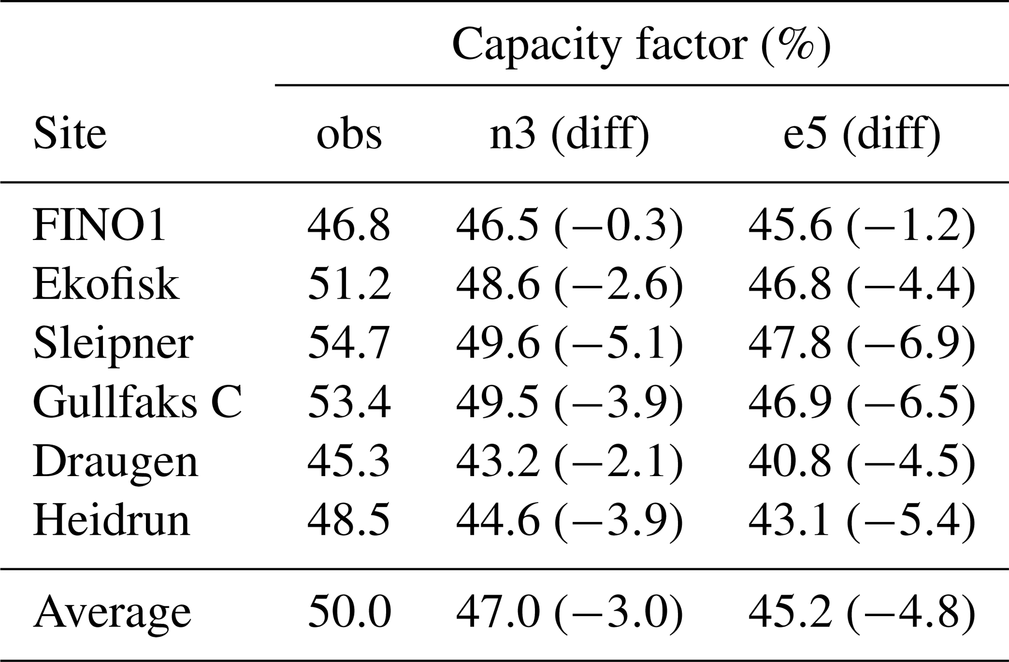
As illustrated in Fig. 2 the largest difference between the observations, NORA3, and ERA5 is found for wind speeds exceeding a typical cut-out limit of 25 m s⁻¹ (u≥u_co). Since the power production is terminated or at least reduced when u≥u_co, we calculate the wind power capacity factors (CF) for the three data sets. This is done to see how the models perform in terms of power production, where the strongest wind speeds are not influencing the result due the power production cut-out limit. Table 4 contains the CF for the observed data, NORA3, and ERA5 for the six sites. NORA3 performs consistently better than ERA5, where NORA3 is on average 1.8 percentage points closer to the average observed CF value compared to ERA5.

The required rate of return when planning offshore wind projects is typically 5 %–10 %. A deficiency of 3 percentage points (approximately 6 % difference in the average power output) in the CF is a sizable error and might be too large in terms of profitability. Nevertheless, this highlights the need for building up archives of different NWP simulations to be able to conduct informed uncertainty calculations for the power production in regions where observational data are limited. However, the comparison of CF between NORA3 and ERA5 shows that the ERA5-based CFs are on average 5 percentage points (approximately 10 % difference in the power output) lower than the observation-based CFs. Hence, the improvements using NORA3 over ERA5 gives more realistic wind power profitability measures.

The validation of wind climatology in NORA3 and ERA5 shows that the downscaling of ERA5 in the process of creating NORA3 has resulted in an improved wind resource data set. The remainder of this study will focus on the validation of NORA3 towards observed wind climatology.

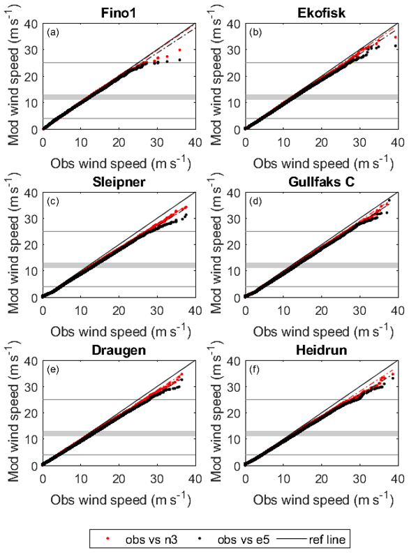
Figure 2 Quantile–quantile plot between the observed wind speed (obs) and the modeled (mod) wind speed, with NORA3 shown in red and ERA5 shown in black, for all the six offshore sites.

Table 4 Capacity factor (%) calculated from the observations (obs), NORA3 (n3), and ERA5 (e5) for the six sites. In addition, the differences (diff) between NORA3 and observations and between ERA5 and observations are also listed.

4 Validation of NORA3 wind speed

Prior to exploiting NORA3 as a wind resource data set in the planning phase of future offshore wind power installations the data set has to be validated and verified against observational data. We start with the validation of mean quantities and wind speed distributions. The most relevant wind speed measures can be seen in Table 5. Arithmetic mean (μ) and standard deviation (σ) are used as measures of the average wind speed and the corresponding variability. Mean wind speeds (μ) for the six sites lie within the interval 10–12 m s⁻¹. For all the sites the observed mean wind speeds are higher than the wind speeds from NORA3, indicating that the model underestimates the mean wind speed. The largest difference can be seen for Sleipner, where the observed mean wind speed is 8.9 % higher than the simulated wind speed. The wind speed at each site is highly variable, with the SD (σ) for the observations varying from 4.7–5.9 m s⁻¹, with the model wind speed being slightly less variable (3 %–8 %). Hence, the observed wind speed is somewhat more intermittent and variable than the modeled wind speed, indicating that HARMONIE-AROME is missing some of the variability embedded in the wind field.

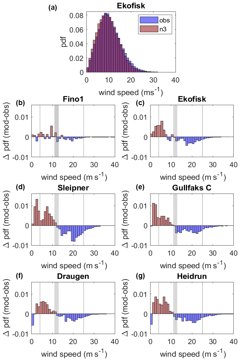
Figure 3 (a) Example wind speed probability density function (pdf) (Ekofisk) for NORA3 (n3) in red and observations (obs) in blue. (b–g) Differences between NORA3 and observational wind speed probability density functions ($\mathrm{\Delta }\mathrm{pdf}={\mathrm{pdf}}_{\mathrm{mod}}-{\mathrm{pdf}}_{\mathrm{obs}}$) for the six sites. When Δpdf=0.01 the probability that the given wind speed will occur is 1 % higher in the model output. The large gray area corresponds to the range within which the rated wind speed usually falls. The gray vertical lines at the left and right mark the cut-in and cut-out wind speed limits used in this study, respectively.

The Weibull scale parameter (“λ” in Table 5) indicates the height and width of the distribution. A larger scale parameter indicates a wider and lower probability distribution. All the observed scale parameters are slightly higher than the modeled; the modeled scale parameters are on average 3.93 % lower than the observed. In other words, the observations contain more wind speed events at the tails of the Weibull distributions, resulting in a larger scale parameter.

As all observed and modeled Weibull shape parameters (“k” in Table 5) are less than 2.6, the distributions are positively skewed, with a long tail to the right of the mean. The observed shape parameter is equal to or smaller than the modeled one (on average 7.3 % lower), indicating that the observed data are more positively skewed with a longer right tail, again emphasizing that the observed data contain more high-wind-speed events than the NORA3 wind speed data.

According to Table 5 the model underestimates the wind speed at all sites. Since the wind power production is a function of the wind speed cubed, the wind power is highly sensitive to systematic deviations between the observed and simulated wind speeds. However, the sensitivity varies with wind speed and is especially strong within the interval between cut-in and rated wind speeds. Figure 3b–h show the differences in the observed and modeled wind speed probability density functions ($\mathrm{\Delta }\mathrm{pdf}={\mathrm{pdf}}_{\mathrm{mod}}-{\mathrm{pdf}}_{\mathrm{obs}}$) for the six sites, in addition to the wind speed distribution for Ekofisk (Fig. 3a). The main finding is that the model underestimates the number of events with high wind speed and overestimates the number of events with low wind speed for all sites. The model is biased towards too few high-wind events and too many low-wind events than observed, and the transition occurs near typical rated wind speeds (11–13 m s⁻¹) for state-of-the-art offshore wind turbines (the widest gray area in Fig. 3b–h). This model bias will have a large impact on the difference between the observed and modeled wind power.

4.1 Wind speed ramp rates

The hourly wind speed ramp rate (m s⁻¹) is a measure of the hourly variability in the data set. In other words, the ramp rate quantifies how much the wind speed changes during 1 h. Figure 4 shows the distributions of observed and modeled hourly wind speed ramp rates for Ekofisk (the other sites have similar distributions). The distribution is wider for the observations than for the modeled data, illustrating that the observed wind speed change from one hour to the next is greater than that in the modeled wind speed data.

Table 5 Statistical measures of the wind speed (m s⁻¹) for the observations (obs) and the model (n3). μ and σ are the arithmetic mean and standard deviation, respectively. λ and k are the Weibull scale and shape parameters, respectively. The wind speed validation is performed at the sensor height to avoid uncertainties related to power law extrapolation (see Table 1 for information on heights).

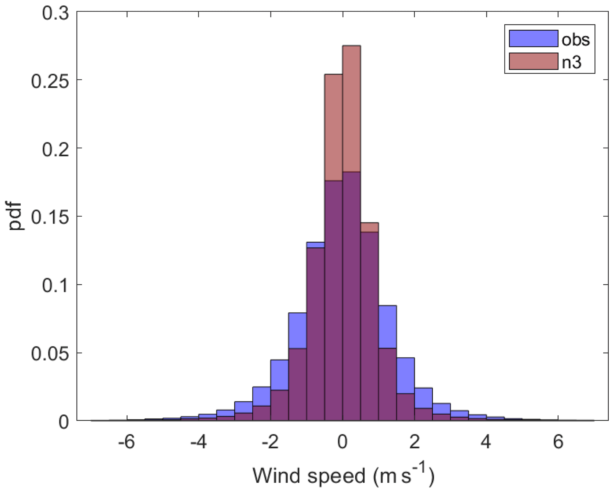
Figure 4 The probability density distribution (pdf) of the modeled (n3) and observed (obs) hourly wind speed ramp rates (m s⁻¹).

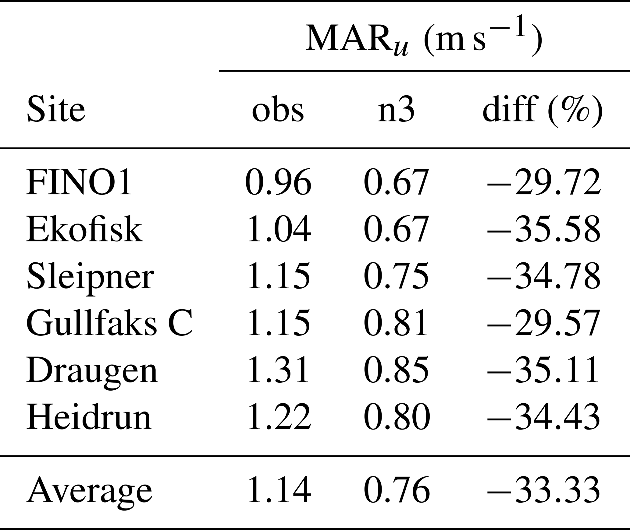
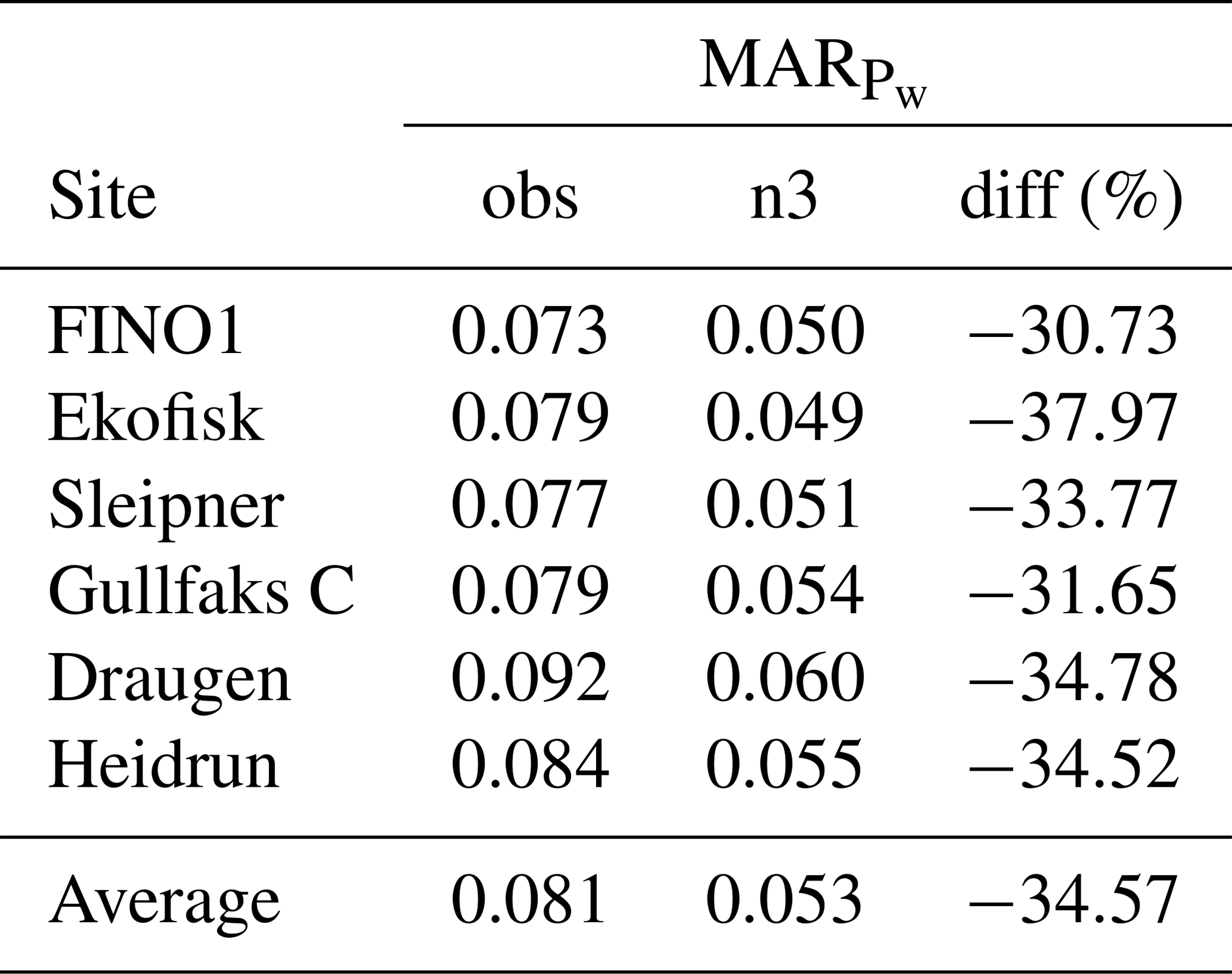
The mean absolute ramp rate (MAR) for the observed and modeled wind speed (u) is shown in Table 6. Typically observed MAR is around 1 m s⁻¹, and the difference between modeled and observed ramp rates indicates that the model underestimates the variability in hourly wind speed by 30 %–36 %.

Table 6 Mean absolute ramp rate (MAR) in meters per second (m s⁻¹) for the observed and modeled wind speed (u). The difference between the modeled and observed MAR_u divided by the observed MAR_u is given as a percentage (%).

4.2 Far-offshore to coastal wind speed gradient

An important feature of a model wind data set is the ability to properly estimate the horizontal wind speed gradient from far offshore to coastal areas. There are limited possibilities to investigate this using the available observational data. However, we made use of data from an observational meteorological mast situated on the coastal island of Frøya (see Fig. 1) to present some indicative results. Generally, using wind speed data at sensor height for the three sites Heidrun (far offshore), Draugen (near coastal), and Frøya (coastal) shows that there is no clear bias in the model (see Table 7). NORA3 underestimates the local far-offshore to near-coastal wind speed gradient but slightly overestimates the near-coastal to coastal gradient.

Table 7 The average change in wind speed (m s⁻¹) at sensor height per 100 km for Heidrun–Draugen and Draugen–Frøya.

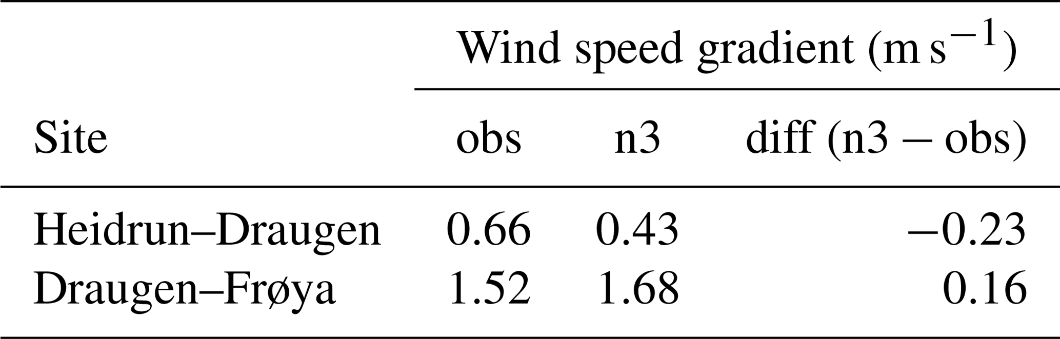
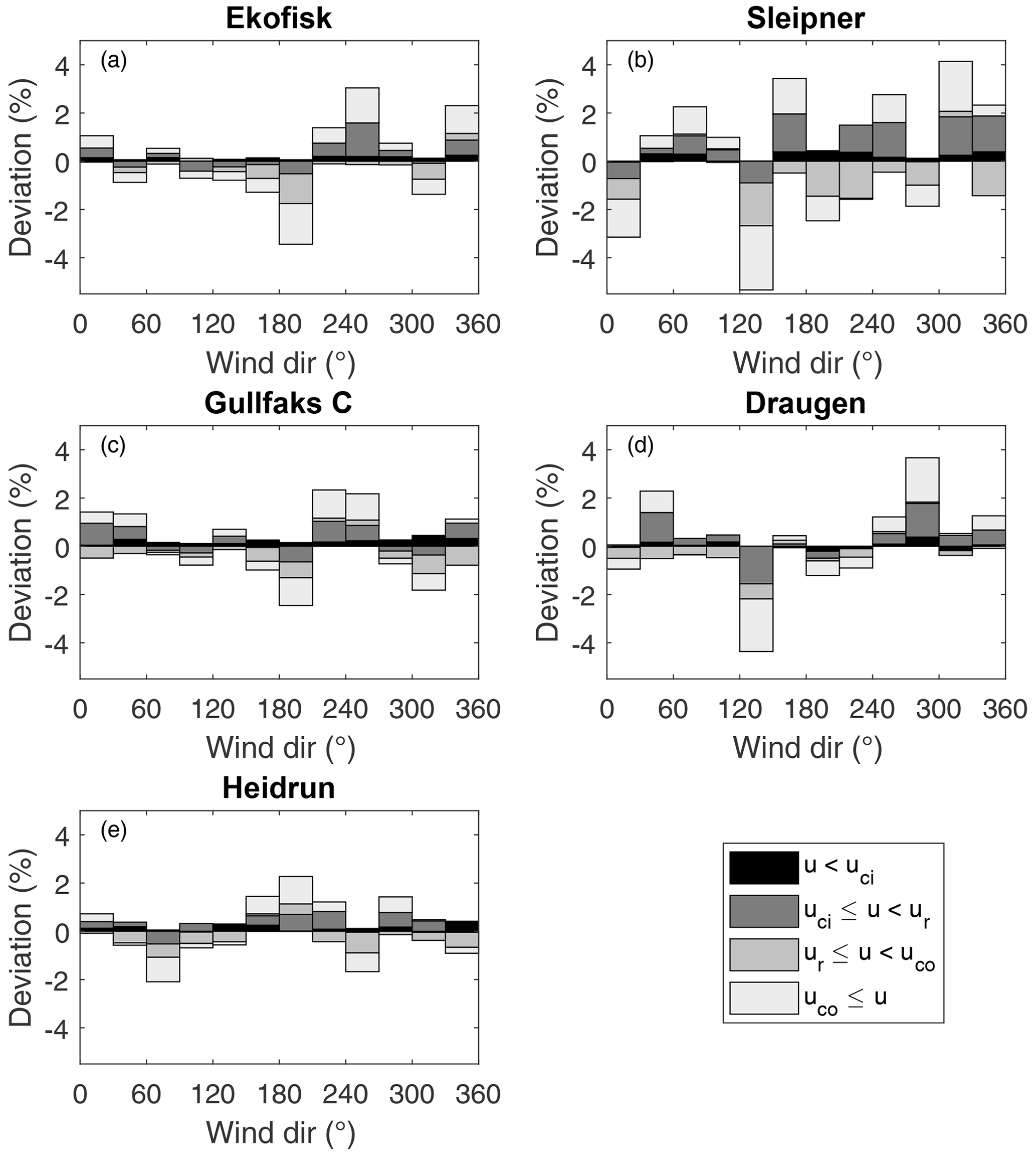
Figure 5 Difference in the occurrence (%) of wind events categorized in different wind direction intervals (30^∘ intervals) between NORA3 and observations (model − obs) for (a) Ekofisk; (b) Sleipner; (c) Gullfaks C; (d) Draugen; (e) Heidrun. For each wind direction interval the wind events are divided into four different wind speed categories, the first one corresponds to u less than cut-in wind speed (u<u_ci), the second is the wind speed interval where the wind power is a function of the wind speed cubed ($u_{\mathrm{ci}}\le u<u_r$), the third interval contain the wind speeds corresponding to rated wind power production ($u_r\le u<u_{\mathrm{co}}$), and the last interval is where the wind speeds are too strong resulting in a terminated wind power production (u_co≤u).

4.3 Wind direction

Another important factor for planning a wind farm using simulated data is the quality of the modeled wind direction. State-of-the-art wind turbine technology allows the wind turbines to yaw to face the main wind direction. Mapping the wind direction climatology is important for the wind farm layout. Wind-rose plots (see Sect. A Fig. A1) demonstrate that the modeled and observed data in general show the same wind direction distributions, with only small differences. FINO1 is excluded from the verification of wind direction because the wind rose for that site shows a clear directional disturbance, as the wind is affected by the observation mast. Figure 5 graphs the differences between the modeled and observed data (%) in the number of wind direction events (30^∘ intervals) for four wind speed categories (u<u_ci, $u_{\mathrm{ci}}\le u<u_r$, $u_r\le u<u_{\mathrm{co}}$, and u_co≤u). There is no systematic bias in wind direction that can be seen across the sites, and the biases in frequency are less than 5 % for all directional intervals and all sites. The wind speed interval with the greatest difference between the model and the observations features wind events corresponding to u≥u_co. The wind speed intervals with the smallest difference between the model and the observation are the too low wind events (u<u_ci). Hence, the model is better at capturing the wind direction when the wind speed is low.

Table 8 Statistical measures of the observation-based (obs) and model-based (n3) normalized wind power production. q₅₀ is the hourly median production, IQR is the interquartile range of the hourly production, and CF is the wind power capacity factor. The wind power measures and estimates are performed at a typical hub height of 100 m a.s.l. using the interpolation of observed wind speeds as outlined in Sect. 2.3 and the power curve given in Sect. 2.4 for all the sites.

Sleipner is the site with the greatest difference between model and observations for almost all wind direction intervals (see Fig. 5b). The mismatch between the observed and modeled wind direction events for Sleipner is probably tied to the model performance. However, we cannot exclude the possibility that the platform design at Sleipner affects the flow field more than the design of the other platforms.

4.4 Uncertainties in observed wind speed

Working with observational data and numerical weather prediction models involves dealing with data that contain uncertainties and errors of known or unknown character. The majority of the observational sites used in this study (five of six sites) are oil and gas platforms. The platforms are large structures that may influence the upcoming flow. On the other side, an observational mast may also influence the flow when the upcoming wind is guided to pass through the mast before being recorded by the sensor.

Flow alteration by structures is a complex issue and might lead to both speedup and slowdown effects of the wind speed but also deflection of the wind vector resulting in a change in wind direction. A potential alteration of the wind would be a function of the platform layout, the atmospheric stability, the upcoming wind direction, and the ambient wind speed. To what extent large offshore structures influence the ambient flow field is unclear (Berge et al., 2009; Vasilyev et al., 2015; Furevik and Haakenstad, 2012). To investigate the distortion caused by these large structures, we compared wind speed data from the platforms with data from FINO1 and from the meteorological mast at the Frøya field station. The result (not shown) indicates that flow disturbance by large oil and gas platforms is to some extent visible in the wind speed and wind direction data for some of the platforms. However, indicating the portion of the wind data difference between the observations and NORA3 that is caused by flow distortion or by the model performance is not possible.

Despite the aforementioned uncertainties, using observations from oil and gas platforms enable us to validate NORA3 over ocean areas where observational data are sparse.

5 Comparison of estimated wind power from observed and modeled wind speed

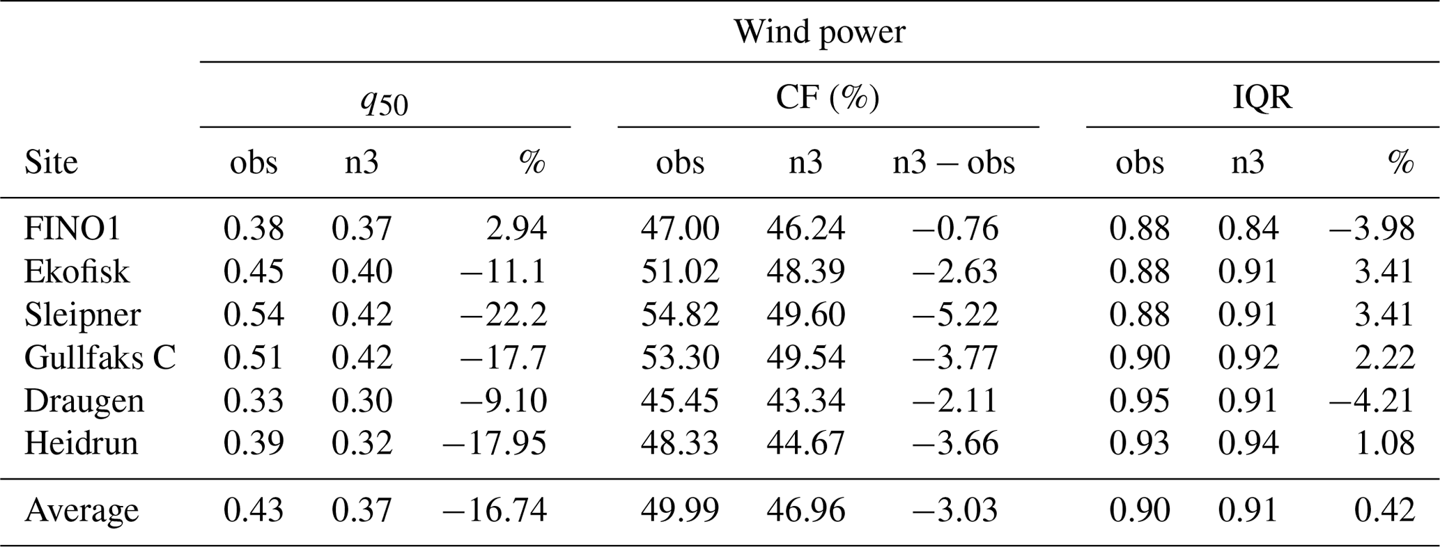
Because the conversion from wind speed to wind power is nonlinear (see Eq. 3), the wind power distribution differs greatly from the wind speed distribution. The statistical measures for the wind power are shown in Table 8. Median (q₅₀) and interquartile range (IQR) are independent of data distribution and are therefore good representations of the average wind power production and the related intermittency, respectively. All wind power estimates are calculated at a hub height of 100 m a.s.l. using the wind interpolation method discussed in Sect. 2.3 and the normalized power curve described in Sect. 2.4.

Both the observation-based and model-based median wind power production estimates reveal very good wind power potential for the six sites (see Table 8). Nevertheless, since the model underestimates the wind speed events exceeding the rated wind speed, this partly counteracts the model's overestimation of the lower wind speed events (u<u_r), making the modeled average power production slightly underestimated. Therefore, the observation-based estimates of the median hourly power production q₅₀ span from 0.3–0.5 (i.e., the median power production for a given hour would typically be 30 %–50 % of installed capacity), compared to 0.3–0.4 for the model-based estimates. IQR, a measure of the variability, is the range between the first and third quartiles (q₇₅−q₂₅). Since the range of the normalized wind power is 0–1, IQR values close to 1 correspond to high variability, since almost the entire data range is present between the first and third quartiles. Hourly IQRs range from 0.86–0.95 for the observation-based estimates and from 0.80–0.94 for the model. There is no systematic difference between the IQRs of the model-based estimates and the observation-based estimates.

The capacity factor (CF) is another statistical measure quantifying the wind power potential. CF is here defined as the average wind power potential divided by the installed capacity. The observation-based estimates of CF vary between 46 % and 55 %, and the CF values from the model-based estimates are slightly smaller. The observation-based CF values exceed the modeled values by an average of 3 percentage points.

5.1 Wind power ramp rates

Figure 6 shows the distribution of observation-based and model-based hourly normalized wind power ramp rates for Ekofisk (the other sites have similar distributions). As for the distribution of hourly wind speed ramp rates, the distributions of hourly wind power ramp rates are wider for the observation-based ramp rates than for the model-based ones, illustrating that the hourly estimated wind power variability based on observations is greater than the estimated variability based on NORA3 data. The difference in MARs indicates an hour-to-hour variability typically of 7 %–9 % (Table 9) of the installed capacity based on observations. In contrast, the variability for model-based estimates is 5 %–6 % and is underestimated at all sites.

Figure 6 The probability density function (pdf) of the ramp rates for observation-based (obs) and model-based (n3) hourly normalized wind power.

Table 9 Mean absolute ramp rate (MAR${}_{{\mathrm{P}}_{\mathrm{w}}}$) for the normalized observation-based and model-based estimates of the wind power output. The difference between the modeled and observed MAR${}_{{\mathrm{P}}_{\mathrm{w}}}$ divided by the observed MAR${}_{{\mathrm{P}}_{\mathrm{w}}}$ is given in percentage (%).

5.2 Inter-annual and seasonal capacity factor

In addition, to encompass short-term variations in wind speed and estimated power production, it is essential for a model data set to contain the correct long-term variations. In this section we evaluate NORA3's ability to capture the longer-term climatic variability of the wind power potential for a given site. The inter-annual and seasonal variations in CF provide a good indication of how NORA3 performs in terms of long-term wind power fluctuations.

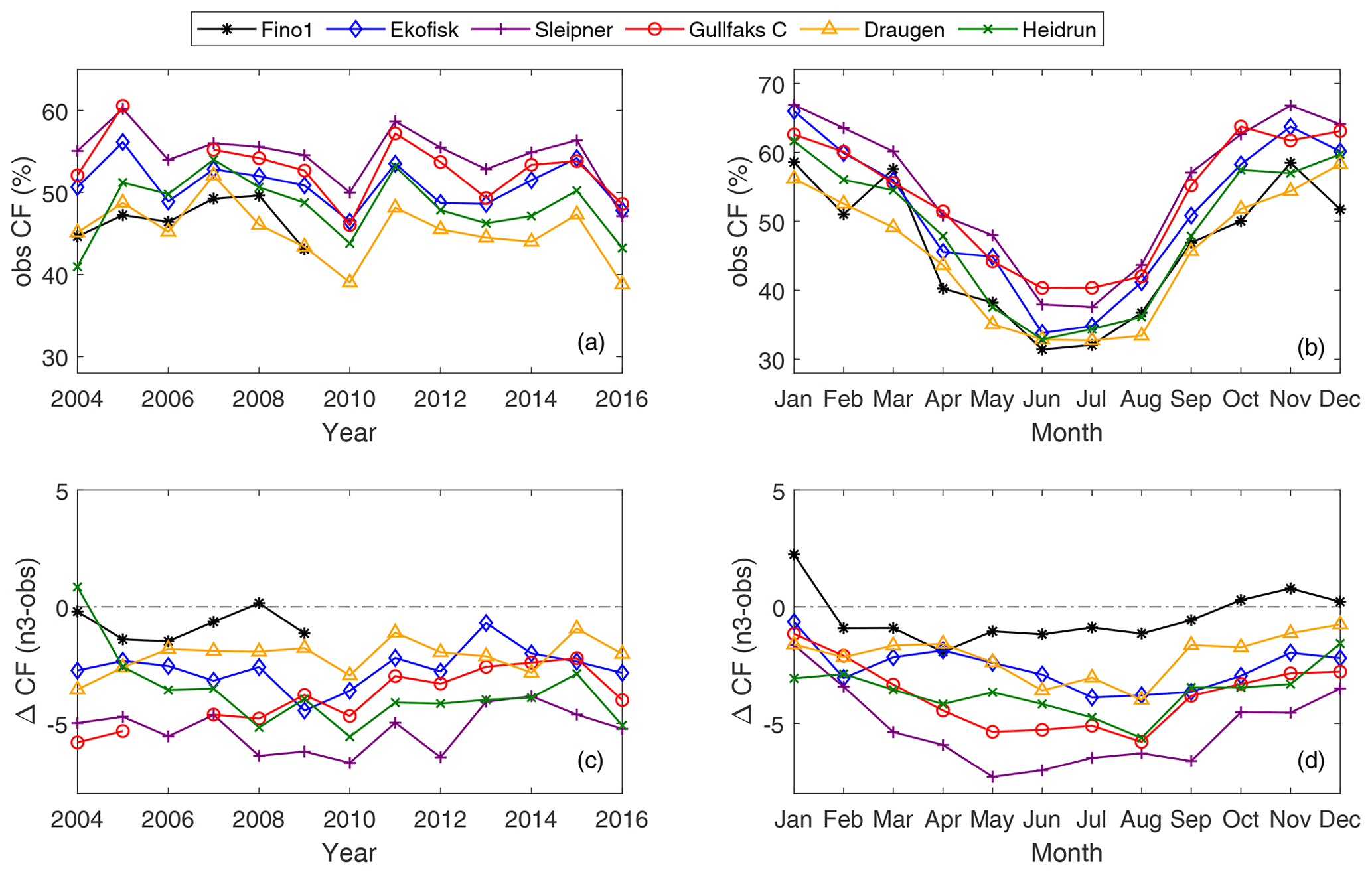
Figure 7 (a) The observed inter-annual variation in the capacity factor (obs CF). (b) Seasonal variation in CF for the observations. (c) The difference in the inter-annual CF (ΔCF) between the model and the observations (n3 − obs). (d) The difference in the seasonal CF between the model and the observations (n3 − obs). A specific year was excluded from the plot if more than one-half of the data for that year were missing.

Figure 7a and b illustrate the inter-annual and seasonal CF, respectively, from the observation-based estimates. In addition, the CF deviations (ΔCF) between the model-based estimates and the observation-based estimates are illustrated in Fig. 7c and d. The observed year-to-year variation in CF is substantial, varying up to 0.12 (12 % of installed capacity) from one year to the next. Figure 7c shows that the yearly CF values from the model are systematically lower than the observed CF values. This result is most pronounced for Sleipner, where the difference in $\mathrm{\Delta }\mathrm{CF}\approx -\mathrm{5}$, meaning that the model-based CF is on average 5 percentage points lower than the observation-based CF.

The model's underestimation of CF can also be seen in the seasonal CF values. Fig. 7d shows that ΔCF<0 for all the sites. The underestimation of the seasonal CF values is largest during the summer months (May–September), meaning that the relative importance of the summer months in wind power production will be slightly underestimated in the model-based estimates.

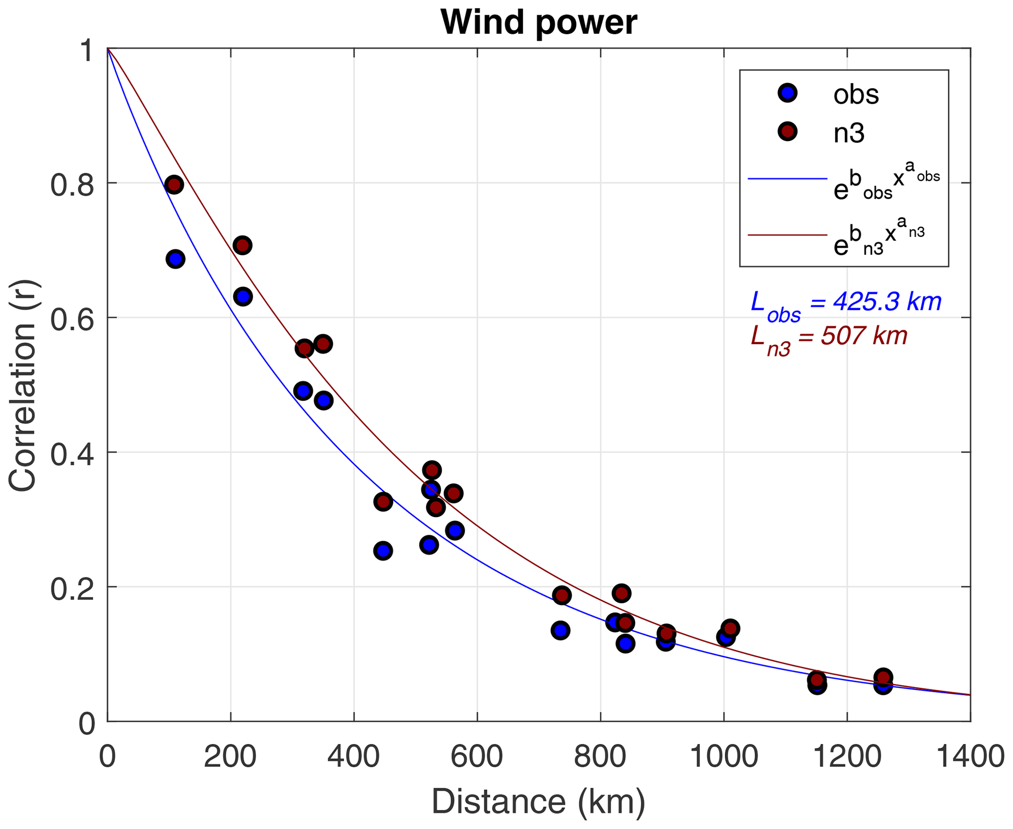
Figure 8 Correlation of wind power time series as a function of the distance between the connected site pairs for the observations (obs, blue) and NORA3 data (n3, red). An exponential fit is also shown ($e^{b{x}^a}$) for both data sets with the corresponding decorrelation lengths, L.

5.3 Spatial wind power co-variability

Many studies have shown that interconnection of wind power production sites mitigates wind power intermittency (Kempton et al., 2010; Reichenberg et al., 2014; St. Martin et al., 2015; Reichenberg et al., 2017; Solbrekke et al., 2020). Therefore, simulated data sets for use in decision-making about future wind power installations should be able to represent spatial and temporal co-variability between wind power sites.

Figure 8 illustrates the ability of NORA3 to capture the spatial co-variance in estimated hourly wind power production between the six sites. The figure demonstrates how the correlation between two sites changes as a function of the separation distance, both for the observation-based estimates (blue) and the model-based estimates (red). For almost all separation distances the model overestimates the correlation between two connected sites. The overestimation is generally small but is greatest for small separation distances. This result indicates that NORA3 is better at capturing the large-scale spatial variability than variance on smaller scales.

5.4 Zero-wind-power events

A general description of the dependency between correlation and separation distance can give us information on the decorrelation length for the sites used in this study. Using the station-pair correlations we identify a best-fitting exponential curve and a decorrelation length L (in kilometers). Connecting sites separated by a distance greater than the decorrelation length ensures that the collective wind power intermittency from the two sites is substantially reduced compared to the intermittency from one of the sites. We use the e-folding distance as a measure of the offshore decorrelation length L. The exponential curves and the corresponding decorrelation lengths for both the observations and NORA3 are presented in Fig. 8. The observation-based L is 425 km compared to a 507 km L based on NORA3. The model-based estimates indicate that to ensure relatively independent hourly power production, a greater interconnection distance is needed than that indicated by the observation-based estimates³.

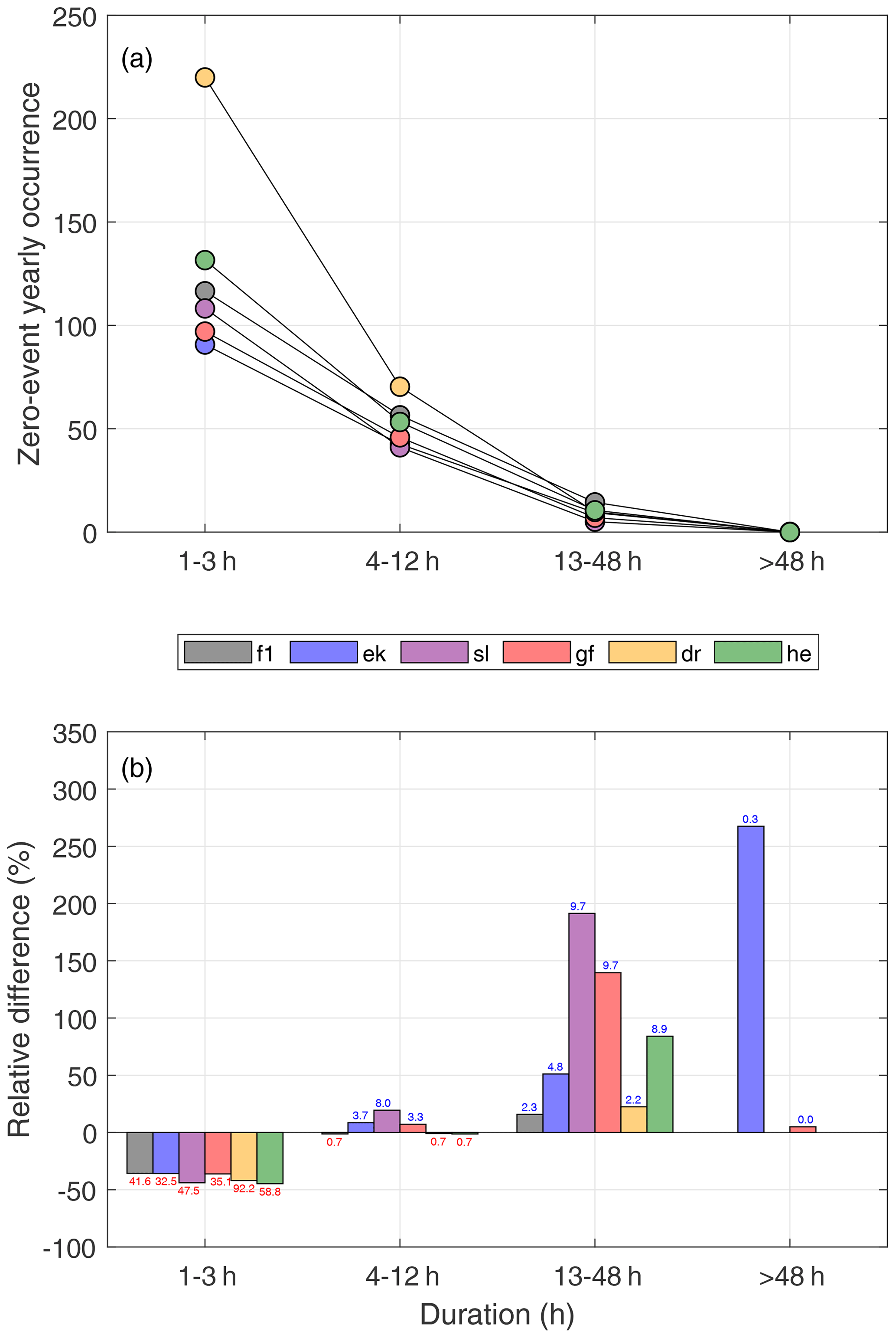
Figure 9 (a) Yearly occurrence and corresponding duration of observation-based zero events caused by wind speeds lower than cut-in wind speed (u<u_ci). (b) The differences between model-based (n3) and observation-based (obs) zero-event occurrences divided by the total number of observed occurrences of too low wind speeds. Values over or under each bar correspond to the differences (n3 − obs) in the number of yearly occurrences between the model and observations. Abbreviations: f1: FINO1; ek: Ekofisk; sl: Sleipner; gf: Gullfaks C; dr: Draugen; he: Heidrun.

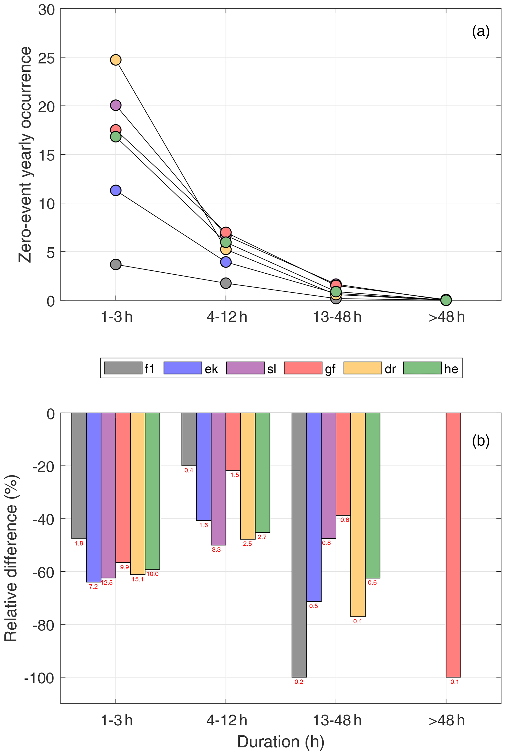
Figure 10 (a) Yearly occurrence and corresponding duration of observation-based zero events caused by wind speeds higher than cut-out wind speed (u≥u_co). (b) The differences between model-based (n3) and observation-based (obs) zero-event occurrences divided by the total number of observed occurrences of too high wind speeds. Values over or under each bar correspond to the differences (n3 − obs) in the number of yearly occurrences between the model and observations. Abbreviations: f1: FINO1; ek: Ekofisk; sl: Sleipner; gf: Gullfaks C; dr: Draugen; he: Heidrun.

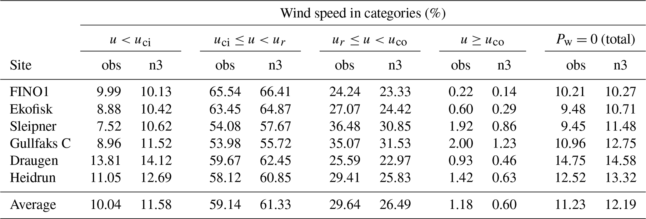
Knowing about the risk, duration, and frequency of zero events (periods of zero wind power production) is important for decision-making and also in turbine maintenance planning, as these measures influence the levelized cost of energy and hence the decision-making process (Cory and Schwabe, 2009). A zero event is caused by a wind speed that is too low (u<u_ci) or too high (u≥u_co), and these events depend to some extent on the technical specifications of a wind turbine but also, and more significantly, on the ambient wind climate in the area of interest. Table 10 shows the percentages of all hourly wind speed values that fall into each wind power category (u<u_ci, $u_{\mathrm{ci}}\le u<u_r$, $u_r\le u<u_{\mathrm{co}}$, and u_co≤u) for each site. In addition, the table lists the total risk of having zero wind power production (P_w=0). The percentage of hours when the wind is too weak to produce wind energy (u<u_ci) ranges from 8 % to 14 % in the observation-based estimates and is overestimated by the model by an average of 1.6 percentage points for all sites. On the other hand, the observation-based estimates indicate that the fraction of hours in which the wind speed is too high (u≥u_co) is about 0.2 %–2 %, and the model underestimates this by approximately 0.6 percentage points. The model's overestimation of the number of hours with winds that are too weak to produce wind power and its underestimation of the number of hours with winds that are too strong results in a well-captured total number of hours of zero wind power production, which differs from the observed value by 1 percentage point.

Table 10 The percentages of observed wind speeds (obs) and modeled wind speeds (n3) that fall into the following four categories: (1) the wind speed is less than the cut-in limit (u<u_ci), (2) the wind speed interval in which the wind power is a function of the cube of the wind speed ($u_{\mathrm{ci}}\le u<u_r$), (3) wind power production is rated ($u_r\le u<u_{\mathrm{co}}$), and (4) wind speed exceeds the cut-out limit (u_co≤u). In addition, the total hours of zero wind power production (P_w=0) divided by the total number of observations are shown as a percentage.

The atmospheric conditions causing winds that are too weak for wind power production are very different from those causing winds that are too strong. Therefore, we split the zero events accordingly. Figures 9 and 10 illustrate the ability of the NORA3 to capture the observation-based estimates of zero events of different duration. Figure 9a shows the observation-based numbers of zero events of varying duration caused by too weak winds. As expected, the number of zero events decreases as the duration of the events increases, ranging from around 90–130 yearly events lasting less than 3 h for most sites to close to zero such events lasting longer than 2 d. Figure 9b graphs the relative differences (in percentage) between the NORA3 and observation-based estimates of the numbers of zero events by duration. The model-based estimates typically have 40 %–50 % too few zero events of short duration (1–3 h) compared to the observations. For longer zero events the model is biased towards too many events.

The model's underestimation of short zero events caused by too low wind speeds and its overestimation of longer zero events occur as a result of the model having lower variability than the observations, as seen in the ramp-rate analysis (see Sect. 5.1). This lower variability means that when these zero events occur in the model they tends to be of longer duration, but the frequency of such events is too low.

From Fig. 10a it is evident that the yearly average occurrence of zero events caused by too strong winds is a factor of 10 lower than the number of zero events caused by winds that are too weak. Hence, one zero event caused by too strong winds happens for approximately every 10 zero events caused by too weak winds. The model underestimates the number of zero events caused by too strong winds for all sites (Fig. 10b); depending on the zero-event duration, NORA3 typically has 40 %–70 % too few zero events caused by too strong winds.

5.5 Expected maximum zero-event duration over the turbine lifetime

In this section we attempt to validate the model's ability to provide reliable estimates of extremely-long-lasting zero events. This is done by estimating the 25-year return value for the duration of a zero event (the typical length of a zero event that statistically would occur at least once over a 25-year period) using the method outlined in Sect. 2.6. Using the Kolmogorov–Smirnov test, we cannot exclude the possibility that the BM data and POT data are drawn from a GEV distribution and a Pareto distribution, respectively. Thus, it is reasonable to fit the observation-based and model-based extreme zero-event duration estimates to these distributions and find the 25-year maximum expected zero-event duration.

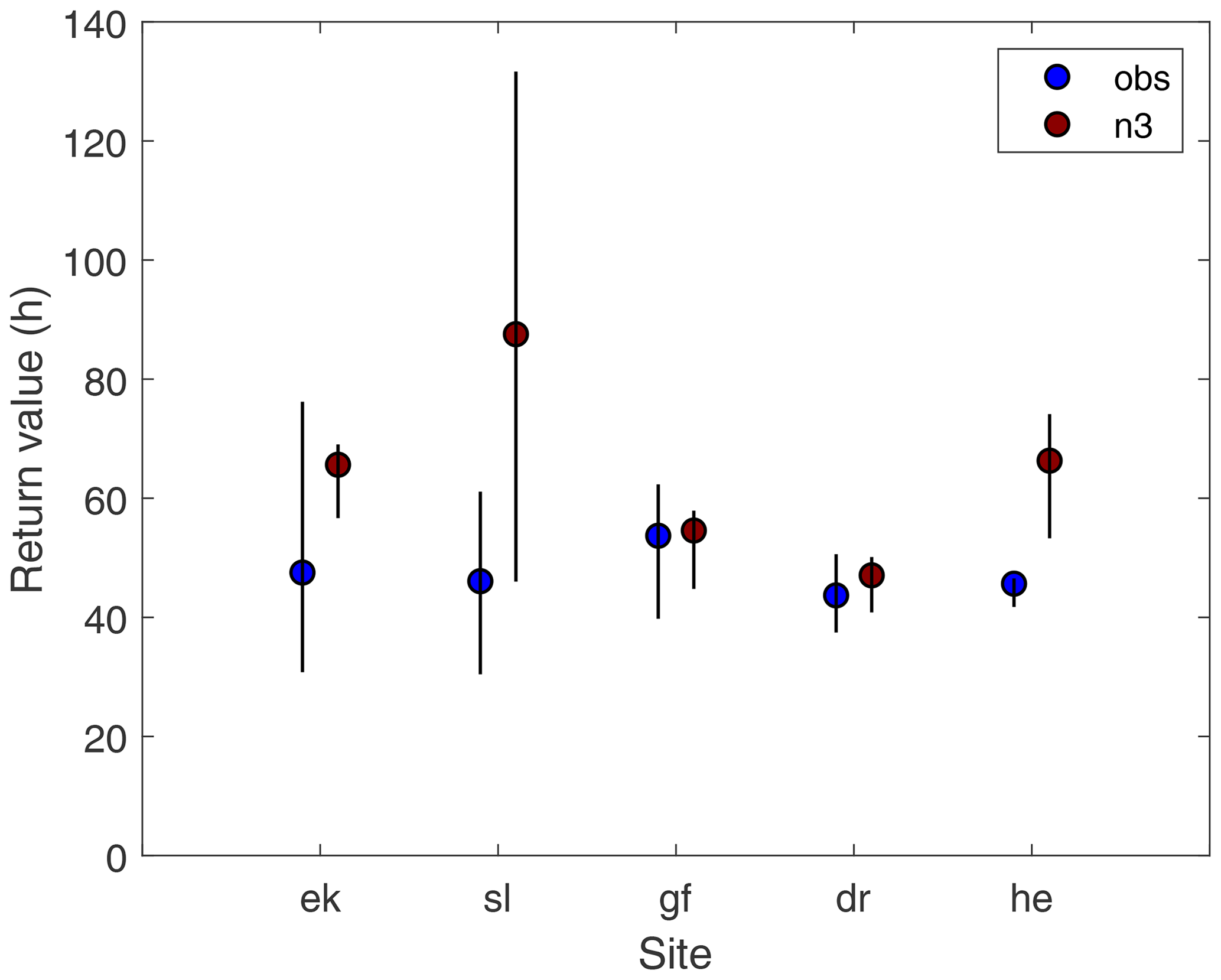
Figure 11 The 25-year return value with the corresponding confidence interval of the maximum duration of a zero event generated by fitting a generalized Pareto distribution to the POT (peak over threshold) data using both observations (obs) and modeled data (n3) for each of the sites. Abbreviations: ek: Ekofisk; sl: Sleipner; gf: Gullfaks C; dr: Draugen; he: Heidrun.

Figure 11 displays the results from fitting the Pareto distribution to the POT data (the results fitting the BM data to the GEV distribution are similar). From the observed data the typical length of the longest zero event expected to occur at least once during the lifetime of a turbine is on the order of 40–60 h, but a zero event of more than 5 d cannot be ruled out. The uncertainty in the estimations makes it difficult to judge which sites have the shortest and longest maximum zero-even duration. Using the model data, the estimates are typically longer than the observation-based estimates (not significant at the 2.5 % significance level for four of five sites) and are in line with the lower variability in the modeled hourly wind speed and wind power as seen in the ramp-rate analysis (see Sects. 4.1 and 5.1). In conclusion, using NORA3 to estimate extreme zero-event duration would lead to a conservative estimate of the return values, and the duration might be overestimated due to the lower variability in the model.

6 Summary

We conduct an in-detail validation of NORA3 offshore wind resource and power production for the time period 2004–2016. NORA3 is a new and freely available high-resolution (3 km) numerical mesoscale weather simulation data set from the Norwegian Meteorological Institute. We perform the validation using observations from six offshore sites along the Norwegian continental shelf. In addition, we quantify the performance of NORA3 against the host reanalysis data set (ERA5). Through advanced statistical measures we validate both the NORA3 wind resource and the related wind power production. Validation measures like arithmetic mean, standard deviation, relative difference between the data sets, temporal correlations, and seasonality of the variables are calculated. In addition, we also include comparison and validation of hourly data distributions, hourly ramp rates, spatial correlation, and analysis on the zero-wind-power events including extreme-value analysis. The general picture is that the NORA3 data are well suited for wind power estimates in the absence of in situ data. Nevertheless, there is a tendency towards the model generating slightly conservative estimates, and the results are summarized below.

The comparison between NORA3 and ERA5 demonstrates that NORA3 outperforms ERA5 in terms of mean and standard deviation of the wind speed climatology for all seasons and for all wind speed intervals, especially for the very strong winds (u≥u_co). Since the very strong winds are not contributing to power production, the average power capacity factors (CF) are also compared. Again, NORA3 differs from the observation-based CF by on average 3 percentage points compared to ERA5's deficiency of 5 percentage points. The validation of wind climatology in NORA3 and ERA5 shows that the downscaling process resulted in an improved wind resource data set.

For all the six offshore sites NORA3 data are biased towards lower mean wind speeds (u_obs=10.64 m s⁻¹, u_n3=10.05 m s⁻¹). The differences in wind speed distribution between the observations and the model output reveal that the model underestimates the number of events with wind speed exceeding the rated wind speed and overestimates the number of events with wind speeds below the rated wind speed (see Fig. 3). The transition between over- and underestimation by the model occurs near typical rated wind speeds (11–13 m s⁻¹). As the model underestimates the wind episodes above the rated wind speed, this partly counteracts the model's overestimation of low wind speeds, making the total modeled power production slightly underestimated.

NORA3 is also slightly biased towards less variable wind speeds on hourly timescales. Analyses of hourly wind speed ramp rates show that the hour-to-hour variability is typically slightly above 1 m s⁻¹, while the model-based ramp rates are slightly below 1 m s⁻¹, resulting in an underestimation of wind speed ramp rates on the order of 30 % (see Table 6).

Generally, estimates of wind power from NORA3 are biased towards too low median values ($P_{\mathrm{w},\mathrm{obs}}=\mathrm{0.43}$, $p_{\mathrm{w},\mathrm{n}\mathrm{3}}=\mathrm{0.37}$) and wind power CFs (CF_obs=50 %, CF_n3=47 %). The negative bias is a consistent feature seen in all years and for all months for all the six sites (except at FINO1 for some months).

The wind power ramp-rate analysis shows that the hourly wind power variability of the NORA3-based estimates is too low. The observation-based wind speed variability leads to a corresponding wind power ramp rate that is typically 0.08 (8 % of installed capacity), while the model-based ramp rate estimated is typically 0.05.

By interconnection of site pairs we demonstrate that the spatial co-variability in estimated hourly wind power production between sites is slightly higher for the NORA3 data than for the observational data. Hence, the decorrelation length is estimated to be 19 % longer in the model-based estimates.

The estimation of the occurrence and duration of zero events shows a well-captured total risk of hourly zero events (n3=12.19 %, obs=11.23 % of the time). We split the zero events into episodes of no wind power production caused by either too low (u<u_ci) or too high (u≥u_co) wind speeds. For zero events caused by winds that are too strong, NORA3 underestimates the occurrence of zero events for all durations. For winds that are too weak, NORA3 underestimates the number of short zero events (1–3 h) but is biased towards an excess of zero events with longer duration. As a result, when a zero event occurs in the NORA3 data, it tends to be of longer duration, but the frequency of such events is too low. This deviation from the observation-based zero events is in line with the lower variability in hourly wind speeds seen in the ramp-rate analysis (Sects. 4.1 and 5.1).

In the extreme-value analysis we found that at least once during the lifetime of a turbine (25 years) a zero-power event is expected to last for 1 to 3 d, depending on the site in question (see Fig. 11). However, a zero event lasting longer than 5 d cannot be ruled out for some sites. Overall, the 25-year return values from NORA3 are somewhat conservative, with a tendency towards longer maximum zero-event duration than seen in the observation-based return values.

To a large degree NORA3 resembles the climatological offshore wind resource and wind power characteristics seen in the observations. However, the model slightly underestimates the wind resource and power potential, and the hourly variability in the model output is lower than in the observations. These characteristics should be kept in mind when using the NORA3 data set in the planning phase of a future offshore wind farm.

Appendix A: Wind direction

See Fig. A1 for the observed and modeled wind-rose plot.

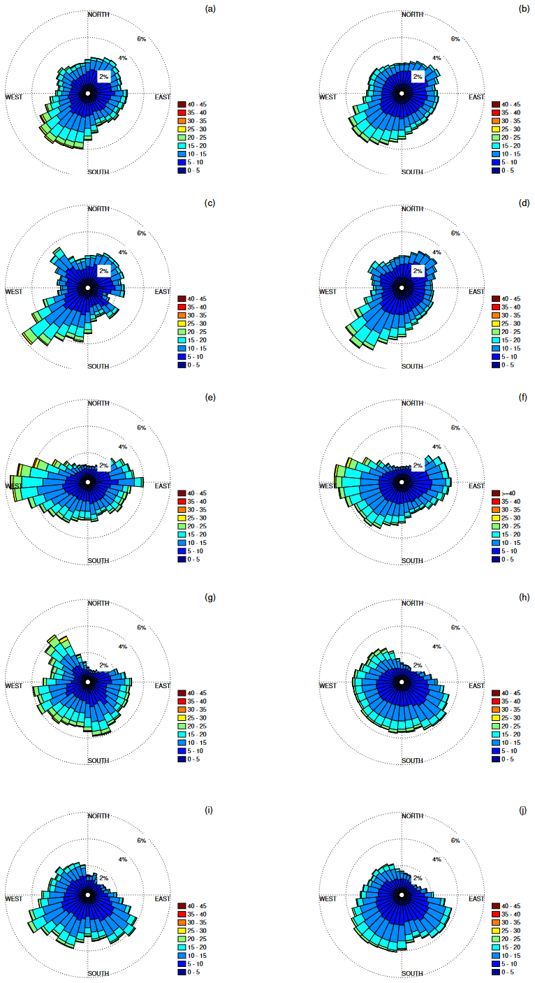
Figure A1 Observed (a, c, g, e, i) and modeled (b, d, f, h, j) wind roses for the five oil and gas platforms. The colors show the wind speed intervals in meters per second. (a, b) Heidrun; (c, d) Draugen; (e, f) Gullfaks C; (g, h) Sleipner; (i, j) Ekofisk.