Utilizing physics-based input features within a machine learning model to predict wind speed forecasting error

Machine learning is quickly becoming a commonly used technique for wind speed and power forecasting. Many machine learning methods utilize exogenous variables as input features, but there remains the question of which atmospheric variables are most beneficial for forecasting, especially in handling non-linearities that lead to forecasting error. This question is addressed via creation of a hybrid model that utilizes an autoregressive integrated moving-average (ARIMA) model to make an initial wind speed forecast followed by a random forest model that attempts to predict the ARIMA forecasting error using knowledge of exogenous atmospheric variables. Variables conveying information about atmospheric stability and turbulence as well as inertial forcing are found to be useful in dealing with non-linear error prediction. Streamwise wind speed, time of day, turbulence intensity, turbulent heat flux, vertical velocity, and wind direction are found to be particularly useful when used in unison for hourly and 3 h timescales. The prediction accuracy of the developed ARIMA–random forest hybrid model is compared to that of the persistence and bias-corrected ARIMA models. The ARIMA–random forest model is shown to improve upon the latter commonly employed modeling methods, reducing hourly forecasting error by up to 5 % below that of the bias-corrected ARIMA model and achieving an R² value of 0.84 with true wind speed.

1 Introduction

Global wind power capacity reached almost 600 GW at the end of 2018 (GWEC, 2019), making wind energy a vital component of international electricity markets. Unfortunately, integrating wind power into an existing electrical grid is difficult because of wind resource intermittency and forecasting complexity. For utility companies employing wind power, it is important to estimate the aggregated load over a period of time to better balance grid resources, including long-term (1+ days ahead), short-term (1–3 h ahead), and very-short-term (15 min ahead) forecasts (Soman et al., 2010; Wu et al., 2012). Forecasting accuracy depends on site conditions, surrounding terrain, and local meteorology. Many wind farms are built in locations which are known to amplify winds due to surrounding terrain (such as Lake Turkana in Kenya, Tehachapi Pass in California, etc.), requiring bespoke forecasts for accurate predictions. Numerical weather prediction models (NWPs) fail at such complex sites due to a lack of appropriate parameterization schemes suitable for local conditions (Akish et al., 2019; Bianco et al., 2019; Olson et al., 2019; Stiperski et al., 2019; Bodini et al., 2020). Therefore, statistical models and computational learning systems (such as an artificial neural network or random forest) are likely better suited to provide accurate power forecasts. Since wind power production is heavily reliant upon environmental conditions, improvements in wind speed forecasting would allow for more reliable wind power forecasts.

If we simplify our wind speed prediction process down to its core (which has no true relation to atmospheric motions), we can imagine a system of atmospheric flow without external forcing. This would result in a constant streamwise wind speed U (i.e., $U_{\mathit{\tau }}=U_{\mathit{\tau }-\mathrm{1}}$; U is streamwise wind speed, τ a time step; this assumes discrete time steps for simplicity). In this case, a persistence or autoregressive forecast would have zero forecasting error and uncertainty. However, uncertainty increases once we add an external force that we may represent by some variable x₁. Now future wind speed may be seen to be $U_{\mathit{\tau }}=f(U_{\mathit{\tau }-\mathrm{1}}$, $x_{\mathrm{1},\mathit{\tau }-\mathrm{1}})$. Assuming the external force is notable in strength and coupled with the inertia associated with winds, the previous autoregressive model will now struggle to predict U_τ because it does not take into account our external forcing $x_{\mathrm{1},\mathit{\tau }-\mathrm{1}}$, resulting in an error ε (ε_τ is abbreviated to ε for simplicity). We can then break down our future wind speed into two parts: $U_{\mathit{\tau }}={\widehat{U}}_{\mathit{\tau }}+\mathit{\epsilon }$, where ${\widehat{U}}_{\mathit{\tau }}$ is our autoregressive forecast that is only dependent on U_τ−1 (i.e., ${\widehat{U}}_{\mathit{\tau }}=f\left(U_{\mathit{\tau }-\mathrm{1}}\right)$). The prediction error is thus skewed to represent the effects of the external force $x_{\mathrm{1},\mathit{\tau }-\mathrm{1}}$ upon U_τ−1.

If we continue to add external forces (x₁, x₂, … x_n; n is the number of external-forcing variables), our atmospheric system becomes much more complex and non-linear due to interactions between forcing mechanisms. We can again obtain our forecasting error as $\mathit{\epsilon }=f(U_{\mathit{\tau }-\mathrm{1}}$, $x_{\mathrm{1},\mathit{\tau }-\mathrm{1}}$, $x_{\mathrm{2},\mathit{\tau }-\mathrm{1}}$, … $x_{n,\mathit{\tau }-\mathrm{1}})$, which we can discretize as $\mathit{\epsilon }={\mathit{\mu }}_{\mathit{\epsilon }}+{\mathit{\epsilon }}^{\prime }$ (μ_ε is the error bias, ε^′ the error fluctuations about μ_ε) given that we have a statistically significant sample size, and the process is stationary. Squaring this equation and taking the average gives us the discretized equation for the mean square error $\stackrel{\mathrm{‾}}{{\mathit{\epsilon }}^{\mathrm{2}}}=\stackrel{\mathrm{‾}}{{\mathit{\mu }}_{\mathit{\epsilon }}^{\mathrm{2}}}+\stackrel{\mathrm{‾}}{{{\mathit{\epsilon }}^{\prime }}^{\mathrm{2}}}$, with $\stackrel{\mathrm{‾}}{{{\mathit{\epsilon }}^{\prime }}^{\mathrm{2}}}$ representing the error variance and overlines denoting the average over all samples (Lange, 2005); $\stackrel{\mathrm{‾}}{{\mathit{\mu }}_{\mathit{\epsilon }}^{\mathrm{2}}}$ represents the bias and may be removed via a simple bias correction. The true concern is the error fluctuation term (ε^′) which constitutes the error variance. Assuming the external-forcing variables (x's) are normally distributed, we can break down $\stackrel{\mathrm{‾}}{{{\mathit{\epsilon }}^{\prime }}^{\mathrm{2}}}$ into two constituents (Ku, 1966):

$$\begin{array}{}\text{(1)}& \stackrel{\mathrm{‾}}{{{\mathit{\epsilon }}^{\prime }}^{\mathrm{2}}}={\mathit{\sigma }}_{x_j}^{\mathrm{2}}{\left({\displaystyle \frac{\partial \mathit{\epsilon }}{\partial x_j}}\right)}^{\mathrm{2}}+\mathrm{2}\left[{\mathit{\sigma }}_{x_j,x_k}{\displaystyle \frac{\partial \mathit{\epsilon }}{\partial x_j}}{\displaystyle \frac{\partial \mathit{\epsilon }}{\partial x_k}}\right],\end{array}$$

where j≠k, ${\mathit{\sigma }}_{x_j}^{\mathrm{2}}$ is the variance of x_j, and ${\mathit{\sigma }}_{x_j,x_k}$ is the co-variance between x_j and x_k (subscript τ removed for simplicity). Unless external forcing (or its coupling with U_τ−1) is minimal, the error is likely highly non-linear and chaotic (i.e., large $\stackrel{\mathrm{‾}}{{{\mathit{\epsilon }}^{\prime }}^{\mathrm{2}}}$). Therefore, it behooves us to discover which forcing mechanisms and atmospheric variables are the best predictors of individual fluctuations ε^′, which we will call “exogenous error”.

Many studies that use machine learning (ML) techniques for wind speed or power forecasting utilize a handful of unadulterated atmospheric variables such as wind speed, pressure, and temperature as input features (Mohandes et al., 2004; Ramasamy et al., 2015; Lazarevska, 2018; Chen et al., 2019). Recently, a handful of investigations have begun to determine which variables may be most useful for these models. Vassallo et al. (2020) showed that invoking turbulence intensity (TI) can vastly improve vertical wind speed extrapolation accuracy. Similarly, Li et al. (2019) showed that TI improves wind speed forecasting on multiple timescales, while Optis and Perr-Sauer (2019) showed that both atmospheric stability and turbulence levels are important indicators for wind power forecasting. Markedly, it has been shown by Cadenas et al. (2016) that multivariate statistical models consistently outperform univariate models for wind speed forecasting. However, to the authors' knowledge, the question of which atmospheric variables are most useful in predicting exogenous error has not been addressed in the literature.

This investigation aims to determine if exogenous error may be, at least in part, predicted via a list of common meteorological measurements by following a methodology similar to that performed by Cadenas and Rivera (2010). The autoregressive integrated moving-average (ARIMA) model first obtains an autoregressive forecast, and the forecasting error is extracted and bias-corrected. A random forest model is then utilized to discover patterns in the exogenous variables (and their relations to the endogenous variable U) that are predictive of exogenous error. The ARIMA–random forest hybrid model so constructed is referred to as the ARIMA–RF model.

This study is not intended to provide a catch-all list of input features that should or should not be used for every future study. Rather, it aims to inform future researchers and industry professionals as to what types of meteorological information must be used as ML inputs to predict the non-linear interactions between various atmospheric forces. Section 2 describes the Perdigão field campaign (the data source for the work), site characteristics, and instrumentation used for data collection. Section 3 provides an overview of the models utilized, testing process, and feature extraction and selection methodology. Section 4 provides testing results and includes a discussion of the obtained results. Finally, conclusions can be found in Sect. 5.

2 Site, data, and instrumentation

Data for this study were taken from the Perdigão campaign, a multinational project located in central Portugal that took place in the spring of 2017 (Fernando et al., 2019). The project site is characterized by two parallel ridges, both about 5 km in length with a 1.5 km wide valley between them. These ridges, which are represented by the elevated contours in Fig. 1, run northwest to southeast and rise about 250 m above the surrounding topography, making the site highly complex and increasing forecasting difficulty. The ridges will be referred to as the northern and southern ridge.

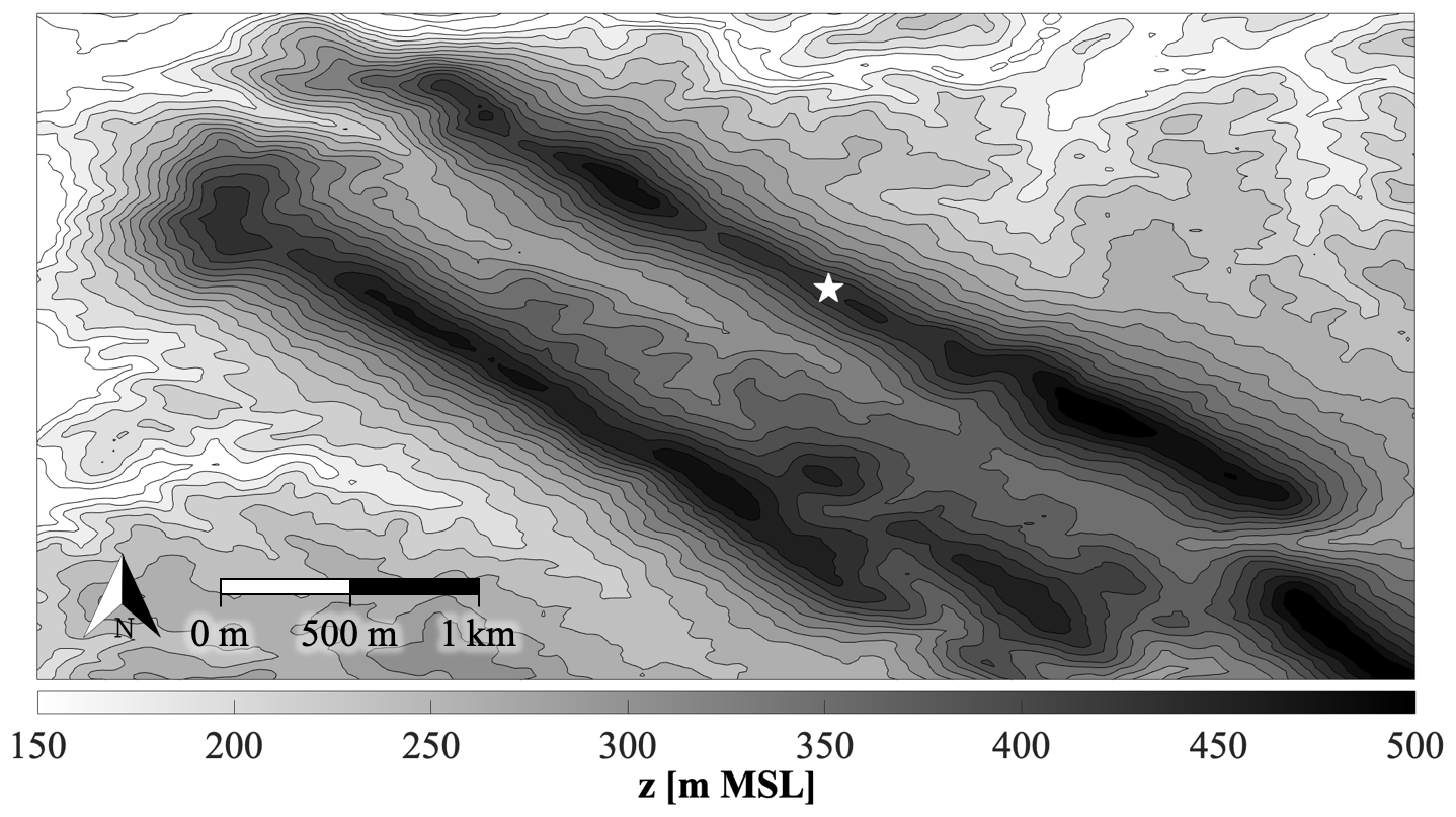
Figure 1 Contour plot of the campaign topography in m a.m.s.l. (meters above mean sea level). The white star represents the 100 m tower location on the northern ridge.

A variety of remote and in situ sensors were positioned in and around the valley to provide an accurate and thorough description of the surrounding flow field. Foremost among these sensors was a grid of meteorological towers which ran both parallel and normal to the ridges. One 100 m tower located on top of the northern ridge (white star in Fig. 1) is utilized in this study. This tower had sonic anemometers (20 Hz native measurement resolution) at 10, 20, 30, 40, 60, 80, and 100 m a.g.l. (above ground level) as well as temperature sensors at 2, 10, 20, 40, 60, 80, and 100 m a.g.l. Information about tower data quality control, including corrections for boom orientation and tilt, may be found in NCAR/UCAR (2019). One of the towers in Perdigão was instrumented with sonic anemometers on both ends of the boom, allowing for an investigation into the effects of tower shadow. Minimal tower shadow effects were observed from the northwest (∼310–340^∘), with a maximum of only 7 % flow deceleration. Wake effects were much smaller than those reported in previous studies (Moses and Daubek, 1961; Cermak and Horn, 1968; Orlando et al., 2011; McCaffrey et al., 2017; Lubitz and Michalak, 2018), which generally exceed 30 %. We have therefore left the data unaltered. The tower data in the Perdigão database have been averaged into 5 min increments by data managers at the National Center for Atmospheric Research (NCAR).

Sensors at 20 and 100 m a.g.l. were chosen because of the high percentage (>99 % for all variables except temperature at 100 m a.g.l., which was available for ∼95 % of the periods) of clean data at these elevations. The utilized data spans 3 months, running from 10 March–16 June 2017. Data at 100 m were correlated with those at 20 m, and missing data were filled using the variance ratio measure–correlate–predict method (Rogers et al., 2005). Any periods unavailable at both heights were filled using linear interpolation with Gaussian noise. All periods are required for proper functionality and assessment of the ARIMA model, and manually filled periods are not expected to make a noticeable difference in the findings.

The quality-controlled data were averaged over 10 min, hourly, and 3 h segments at a 5 min moving average in order to create three robust datasets, each consisting of over 28 000 samples. These three datasets were split via stratified 10-fold cross-validation (Diamantidis et al., 2000). The target streamwise wind speed, or that to be forecasted, is located at 100 m a.g.l. Squared buoyancy frequency (N²), Richardson numbers (flux Ri_f and gradient Ri_g), and temperature gradient ($\frac{\partial T}{\partial z}$) were calculated between 20–100 m a.g.l. Friction velocity (u^*) was found at 20 m, just above surface roughness height (Fernando et al., 2019). All other input variables utilized were from 100 m a.g.l.

3 Methodology

This investigation utilizes two modeling methods, ARIMA and random forest regression, to create a hybrid model (ARIMA–RF) wherein the ARIMA model is first used to get a linear, univariate wind speed forecast. The ARIMA forecast is bias-corrected, and the exogenous error ε^′ is then extracted and used as the target variable for the random forest. The random forest's goal (and the goal of the study) is to predict ε^′ (predictions denoted as ${\widehat{\mathit{\epsilon }}}^{\prime }$) and determine which atmospheric variables and forcing categories are useful for the predictive process. After the most important variables have been established, combinations of these input features are tested in an effort to determine whether specific groupings of input features may provide similar (or improved) forecasts compared to tests which incorporate all inputs. Finally, the ARIMA–RF results are compared with those of the persistence and bias-corrected ARIMA (hereafter referred to as the BCA) models. Section 3.1 details the ARIMA model, while Sect. 3.2 describes random forest regression. Section 3.3 and 3.4 provide more detail on the feature extraction and selection methodology as well as the testing procedure.

3.1 ARIMA

ARIMA (Box et al., 2015) is a univariate statistical model used for time series forecasting. It is predicated on the combination of three functions: an autoregressive function that uses lagged values as inputs, a moving-average function that uses past forecasting errors as inputs, and a differencing function used to make a time series stationary. In its simplest form, the next term in a time series sequence, y_τ, is given by

$$\begin{array}{}\text{(2)}& y_{\mathit{\tau }}=\sum _{i=\mathrm{1}}^p{\mathit{\varphi }}_i{y}_{\mathit{\tau }-i}+\sum _{j=\mathrm{1}}^q{\mathrm{\Theta }}_j{\mathit{\epsilon }}_{\mathit{\tau }-j}+{\mathit{\epsilon }}_{\mathit{\tau }},\end{array}$$

where p and q are the orders of the autoregressive and moving-average functions, respectively; ϕ_i and Θ_j the ith autoregressive and jth moving-average parameters, respectively; y_τ−i the ith lagged value; ε_τ−j the jth past prediction error; and ε_τ the error term at time τ. The order of differencing is given by the parameter d and does not show up directly in Eq. (2).

The dataset was tested for long-term statistical stationarity via the Augmented Dickey Fuller Test (Dickey and Fuller, 1979) using the statsmodels Python module (Seabold and Perktold, 2010). The test, to a statistically significant degree, proved that the wind speed data contain no embedded trends or drift (e.g., changes in the mean or variance of the wind speed due to long-term variability). Therefore, the differencing parameter d was set to 0 (this turns the ARIMA model into an ARMA model, but we stick with the term ARIMA for uniformity). The autoregressive and moving-average parameters used, p=2 and q=1, were determined via minimization of the Akaike information criterion (Shibata, 1976) and empirical testing. Increasing parameters beyond this point did not lead to improved ARIMA accuracy.

3.2 Random forest regression

Random forest regression (Breiman, 2001) is an ensemble method that is made up of a population of decision trees. Bootstrap aggregation (bagging) is used so that each tree can randomly sample from the dataset with replacement, while only a random subset of the total feature set is given to each individual tree. The trees can be pruned (truncated) to add further diversification. After construction, the population's individual predictions are averaged to give a final prediction of the target variable. Ideally, this process results in a diversified and decorrelated set of trees whose predictive errors cancel out, producing a more robust final prediction.

An advantage of random forests is their ability to determine the importance of all input features for the predictive process. This is done by calculating the mean decrease impurity or the decrease in variance that is achieved during a given split in each decision tree. The decrease in impurity for each input feature can be averaged over the entire forest, providing an approximation of the feature's importance for the prediction (feature importance estimates sum to 100 % to ease interpretability). To assist the random forest in representing the dynamic nature of atmospheric processes, input variables are taken from the previous two time steps (i.e., input feature U comprises U_τ−1 and U_τ−2).

The constructed random forest model contains 1000 trees for tests of individual variables and 1500 trees for tests of variable combinations. To ease concerns of overfitting, each internal node was required to have at least 100 samples in order to split (this truncation is a form of regularization). The random forest model was built using the scikit-learn Python library (Pedregosa et al., 2011).

3.3 Feature extraction and selection

In an effort to ensure that the findings are applicable to real-world campaigns, we limit our sources of information to those which may be measured by a typical meteorological mast containing sonic anemometers alongside temperature sensors. Using this information, we can write our future wind speed U_τ as a function of the following variables, which were broken down into their mean and fluctuating values:

$$\begin{array}{}\text{(3)}& U_{\mathit{\tau }}=f\left(U_i,{\mathit{\theta }}_i,W_i,T_i,t_i,u_i^{\prime },{\mathit{\theta }}_i^{\prime },w_i^{\prime },T_i^{\prime }\right),\end{array}$$

where U_i and θ_i are the mean streamwise wind speed and direction, respectively; W_i the mean vertical wind speed; T_i the mean temperature; t_i the time of day; $u_i^{\prime }$ the fluctuating horizontal velocity; ${\mathit{\theta }}_i^{\prime }$ the fluctuating wind direction; $w_i^{\prime }$ the fluctuating vertical velocity; and $T_i^{\prime }$ the fluctuating temperature at each previous time step i. Unfortunately, θ^′ was not available within the dataset utilized (which had already been 5 min averaged) and is therefore ignored for this study. Previous analysis, however, has shown that θ^′ varies inversely with U in complex terrain (Papadopoulos et al., 1992), and we may therefore assume its influence is largely captured by U.

Although these unadulterated features give us an idea as to how the system is working at the moment, they may not explicitly represent the relevant atmospheric forcing mechanisms. Our list of measurements allows us to break down our system into two principal forcing components: buoyancy and inertial forcing (which indirectly includes pressure gradient forces). Each of these forces can be further discretized into large and small scales (also called mean and fluctuating values, typically separated by at least 1 order of magnitude).

Figure 2 shows an illustrative breakdown of the two main forcing mechanisms alongside a list of extracted descriptor variables. The definitions and formulations of all non-obvious extracted variables used in this study can be found in Appendix A. From this figure, it is clear that the variables in Eq. (3), when manipulated, are able to describe both the inertial and buoyant forces at multiple scales. Large-scale inertial forcing can be described by the local mean wind speed (U) and direction (θ; broken down into north–south and east–west components in an attempt to eliminate any discontinuities) or vertical velocity W, while small-scale inertial forcing can be described by variables such as the fluctuating (standard deviation of) velocity σ_u, friction velocity u^*, and the turbulence kinetic energy (TKE). Likewise, large-scale buoyancy forcing can be described by the squared buoyancy frequency N², the temperature gradient ${}^{\partial T}{/}_{\partial z}$, or proxy values such as the time of day t (broken down into sine and cosine components, one of which relates to 00:00–12:00 LT (local time) and the other to 06:00–18:00 LT) or temperature T (which, on average, is higher during the day and lower at night; stability parameters based on Monin–Obukhov similarity theory have been considered ill-suited for complex terrain flows because of the breakdown of underlying assumptions (Fernando et al., 2015) and hence were not used in this study). Small-scale buoyancy effects can be described by the turbulent heat flux $\stackrel{\mathrm{‾}}{w^{\prime }{T}^{\prime }}$. The correspondence between forces and internal parameters can also be described by non-dimensional variables such as the gradient Richardson number Ri_g, flux Richardson number Ri_f, turbulence intensity TI, and normalized friction velocity ${}^{u^{*}}{/}_U$. These derived non-dimensional variables, or extracted features, are typically ignored by current ML models in lieu of raw features such as those listed in Eq. (3).

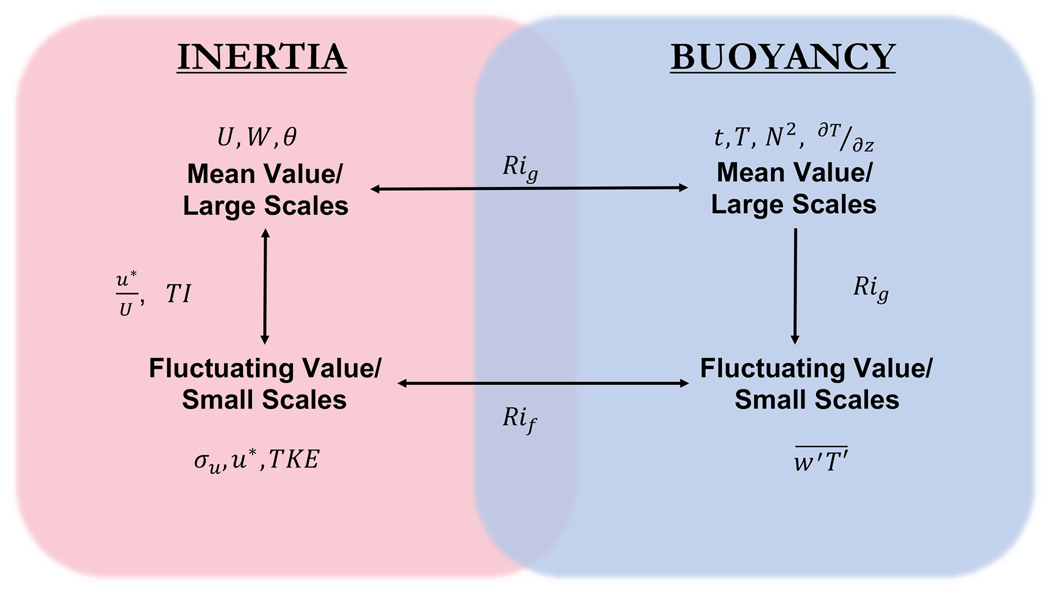
Figure 2 Illustrative breakdown of the scales and variables related to inertial and buoyant forcing; θ^′ is not shown as it is not utilized in the analysis.

Extracted variables like those in Fig. 2 may not provide any more information than the raw variables in Eq. (3). However, they may ease the burden on the model by discretizing (or directly relating) informational categories, therefore reducing informational overlap and noise, providing more periodic patterns, and more accurately describing the underlying system. Further, such well-conceived meteorological variables have been shown to be useful for atmospheric prediction (Kronebach, 1964; Li et al., 2019; Bodini et al., 2020). In theory, given enough data, the model should be able to decipher and interpret these extracted features on its own. Unfortunately there often is not enough collected data for this to happen organically. Instead, by providing better information we can create a simpler, cheaper, more robust model that requires less training data and construction time. Selected features will ideally represent the underlying system as accurately as possible without providing noisy or redundant information.

3.4 Testing

Initial tests utilize a full feature set (i.e., all input variables are included). Feature importance estimates are then extracted from the random forest model, and various user-selected combinations of the most important input features are tested. It must be noted that only select input feature sets were tested in this investigation due to the sheer multitude of potential feature sets.

In order to relieve any timescale bias, forecasts are made across multiple timescales. Typically, wind power utility operators require single-step short-range power forecasts run hour by hour for a few days to reduce unit commitment costs. The forecast skill of observation-based methods generally reduces with forecast lead time within 1 h, and numerical models have higher skill in forecasting larger lead times (>3 h; Haupt et al., 2014). Statistical learning methods have proved to be particularly effective from about 30 min to approximately 3 h ahead (Mellit, 2008; Wang et al., 2012; Yang et al., 2012; Morf, 2014), and roughly this time frame is thus the focus for this study. The shortest forecast predicts wind speeds 10 min ahead, roughly within the turbulent spectral band (Van der Hoven, 1957). Forecasts are also made 1 and 3 h ahead, which are within the spectral gap between the turbulent and synoptic spectra and approach the 6 h period wherein NWP models become particularly useful (Dupré et al., 2019). These are all single-step forecasts, which is to say that the averaging timescale increases with the forecasting timescale (e.g., a 10 min forecast predicts 10 min averaged wind speed, whereas a 3 h forecast predicts 3 h averaged wind speed). Each dataset is split via stratified k-fold cross-validation (Diamantidis et al., 2000), a technique that splits the dataset into k sections (in this case, we set k=10) and uses each section as a separate test set (i.e., tests consist of 10 runs, each of which utilizes a unique test set). This technique splits data nearly chronologically, ensuring that the model does not overfit the dataset. Forecasting metrics for each test are obtained by averaging the ensemble of all 10 runs.

The root mean square error (RMSE) and mean absolute error (MAE) of the BCA are found for each timescale, giving two metrics of the true exogenous error ε^′. The random forest model is then trained to predict ε^′, combined with the ARIMA model, and the newly constructed ARIMA–RF is used to forecast wind speeds. The reduction in RMSE and MAE (which come exclusively from the random forest's prediction of exogenous error ${\widehat{\mathit{\epsilon }}}^{\prime }$) is then found for the test set. Equations (4) and (5) describe both metrics, wherein U_m is the target wind speed, ${\widehat{U}}_{\mathrm{m}}$ the predicted wind speed, m each individual sample, and M the sample size.

$$\begin{array}{}\text{(4)}& {\displaystyle }& {\displaystyle }\mathrm{RMSE}=\sqrt{{\displaystyle \frac{\mathrm{1}}{M}}\sum _{m=\mathrm{1}}^M{\left(U_{\mathrm{m}}-{\widehat{U}}_{\mathrm{m}}\right)}^{\mathrm{2}}}\text{(5)}& {\displaystyle }& {\displaystyle }\mathrm{MAE}={\displaystyle \frac{\mathrm{1}}{M}}\sum _{m=\mathrm{1}}^M\left|U_{\mathrm{m}}-{\widehat{U}}_{\mathrm{m}}\right|\end{array}$$

4 Results and discussion

The ARIMA–RF model utilizing the full feature set obtained lower RMSE than the BCA for all timescales. Figure 3 shows a comparison between the RMSE obtained by the ARIMA–RF model and that obtained by the persistence and BCA models. The BCA's RMSE amounted to 0.726, 1.132, and 1.575 m s⁻¹ for the 10 min, hourly, and 3 h forecasts, respectively. The ARIMA–RF, utilizing all input features, reduced these RMSE values (as well as the MAE values) by ∼2 %, 4 %, and 11 %, respectively (RMSE and MAE values given in Table 1). The random forest is clearly able to ascertain more prudent physical patterns at larger timescales (up to 3 h) as large-scale atmospheric dynamics provide a more predictable signal for the prediction of exogenous error.

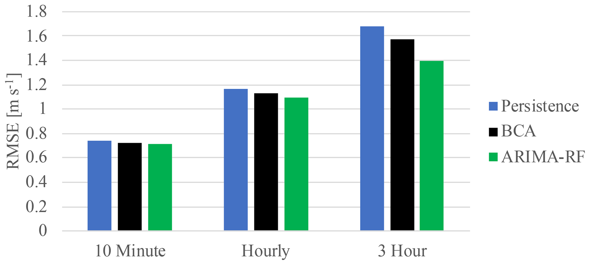
Figure 3 Comparison of RMSE obtained by the persistence, BCA, and ARIMA–RF with the full input feature set for all forecasting timescales.

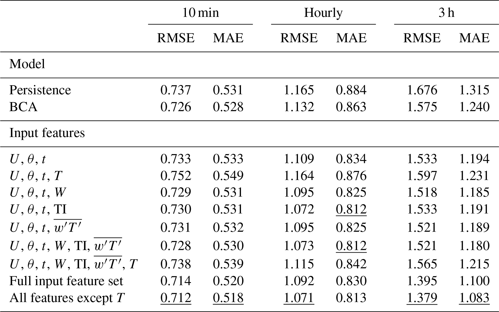
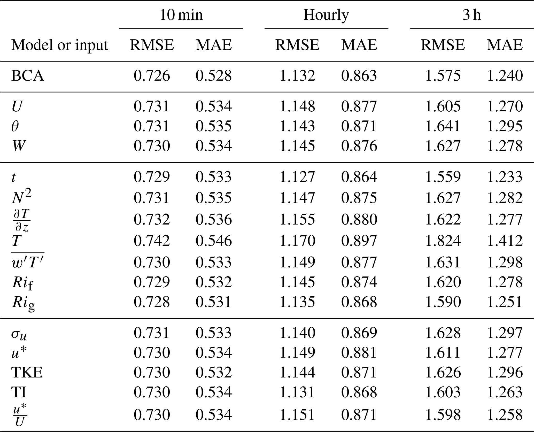
Table 1 RMSE and MAE (m s⁻¹) obtained by the persistence, BCA, and ARIMA–RF models when utilizing select input feature combinations. The final two rows show the testing results when utilizing the full input feature set and the full feature set except T. Underlined values show the best performance from each column.

All feature importance values were extracted from the random forest and are shown in Fig. 4. The variables are broken down into three distinct categories: inertial (large-scale dimensional variables signifying inertial forces in Fig. 2), stability (blue and purple regions in Fig. 2 which are akin to atmospheric stability), and turbulence variables (small-scale and non-dimensional inertial variables in Fig. 2); θ is the most important variable for the prediction of ε^′ at all timescales, achieving up to 20 % importance at the 3 h timescale. Figure 5a shows the partial dependence on the east–west component of θ (i.e., the random forest model's average predictions, ${\widehat{\mathit{\epsilon }}}^{\prime }$, across the range of a given variable, in this case the east–west component of θ) alongside the variable's distribution. The model is clearly able to discern an east–west directional pattern in the training data. The climatology above the Perdigão ridges displays a proclivity for northeasterly and southwesterly flows, the former of which exhibit comparatively high velocities (Fernando et al., 2019). The BCA tends to underpredict flow from the northeast (i.e., the random forest's average target variable $\stackrel{\mathrm{‾}}{{\mathit{\epsilon }}^{\prime }}$ is positive; Fig. B1, Appendix B). Accordingly, the random forest predicts positive ε^′ values, correcting for the BCA's underprediction. Figure 6c, which displays both the ARIMA–RF (solid lines) and BCA (dashed lines) RMSE values by directional sector, shows that the ARIMA–RF successfully improves hourly and 3 h forecasting accuracy when winds are northeasterly.

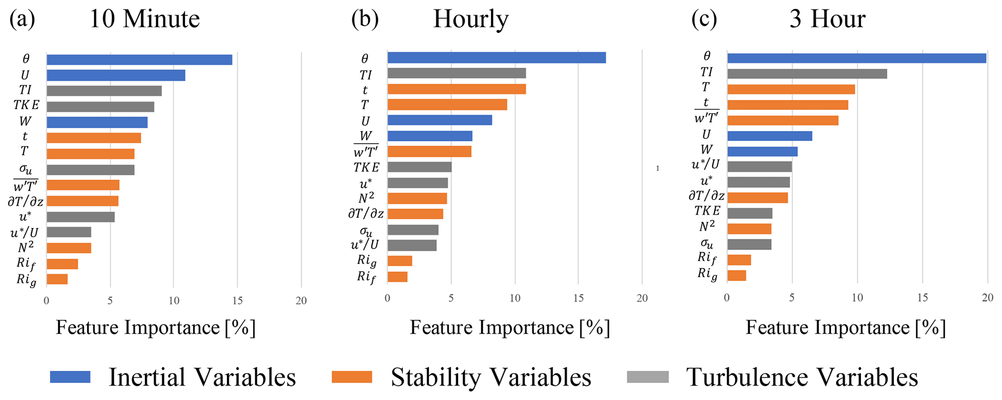
Figure 4 Feature importance for the prediction of exogenous error when all input features are given to the random forest model. Panel (a) shows importance for the 10 min prediction, panel (b) shows importance for the hourly prediction, and panel (c) shows importance for the 3 h prediction. Blue bars denote inertial variables, orange bars denote stability variables, and gray bars denote turbulence variables. Importance values for each test sum to 100 %.

Even larger improvement is seen for westerly winds which pass over the southern ridge prior to reaching the measurement location (Fig. 6c). Westerly winds are common between 13:00–21:00 LT (Fernando et al., 2019), and Fig. 6b shows that the ARIMA–RF is able to improve upon the BCA forecast during these hours. The BCA tends to overpredict wind speeds around 12:00 LT (i.e., negative $\stackrel{\mathrm{‾}}{{\mathit{\epsilon }}^{\prime }}$ in Fig. B2, Appendix B), as wind speeds reach a relative nadir (Fernando et al., 2019). The model's overprediction is captured and partially corrected by the random forest, which predicts negative ε^′ values around noon ($t\approx -\mathrm{1}$ in Fig. 5c). Wind speeds then pick up throughout the afternoon as the atmosphere becomes more convective. Increased convection leads to high TKE and TI values, which peak in the mid-afternoon (not shown). As wind speeds rise and the atmosphere becomes more convective, the BCA begins to underpredict wind speeds. The underprediction is once again captured by the random forest, and the artifacts can be seen in Fig. 5b and c. The random forest identifies periods more than 5 h from noon ($t\ge -\mathrm{0.25}$ in Fig. 5c) and those with high TI as periods wherein the BCA will likely underpredict wind speeds, and it corrects the BCA forecast accordingly by predicting positive ε^′ values.

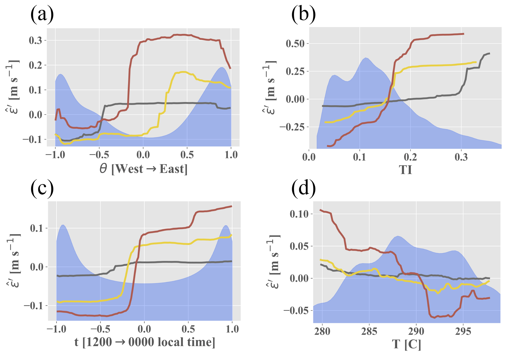
Figure 5 Lines show dependence between the random forest prediction ${\widehat{\mathit{\epsilon }}}^{\prime }$ and (a) the east–west component of θ, (b) TI, (c) the noon–midnight component of t, and (d) T. Blue shading shows variable distribution. Arrows in (a) and (c) correspond to direction (on the x axis) of the normalized oscillatory component.

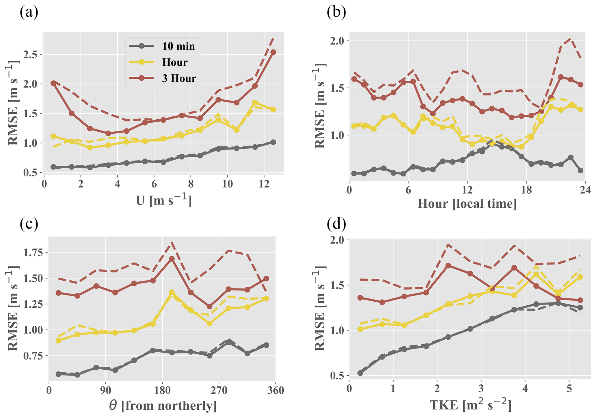
Figure 6 RMSE obtained by the ARIMA–RF (with the full feature set; solid lines with points) and BCA (dashed lines) partitioned by (a) U, (b) hour of the day (local time), (c) θ, and (d) TKE.

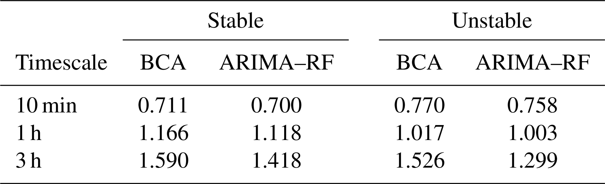
A comparison of both the BCA and ARIMA–RF models' RMSE values in stable and unstable conditions (Table 2) shows that the BCA performs better under unstable conditions for both the hourly and 3 h forecasts, but the opposite is true for the 10 min timescale. Increased turbulence during the daytime clearly hampers the BCA when forecasting 10 min and, to a lesser extent, 1 h ahead (dashed gray and yellow lines, respectively, in Fig. 6d). Notably, the random forest is only able to make minimal forecasting improvements (∼1.5 %) on the 10 min and hourly timescales during unstable conditions but is able to improve the 3 h forecast by almost 15 % during such conditions. Wind speeds can be highly chaotic during convective conditions, leading to large fluctuations as high-energy eddies pass through the measurement location. Typically the large-eddy turnover timescale for the lower atmosphere is 10–20 min (specifically during daytime), and averaging timescales approaching or less than this timescale exclude information on more stable and deterministic large eddies, thus making predictions more prone to random errors. The lack of large-eddy influence results in a wind speed signal that is replete with random fluctuations originating in the inertial subrange, adding substantial noise to the prediction. These fluctuations may overwhelm the ML model's pattern recognition capabilities, even up to the hourly timescale, reducing the random forest prediction to a noisy guess. Such ML models will always make predictions based on patterns in the training data, even when those patterns are erroneous and do not hold for the testing dataset. This results in error predictions that are only minimally correlated with the true exogenous error.

Table 2 RMSE (m s⁻¹) obtained by the BCA and ARIMA–RF (with the full input feature set) based on stability (as defined by N²) of the forecasted time period.

The highest RMSE values produced by the hourly and 3 h BCA occur during the evening transition period (Fig. 6b; sunset typically between 20:00–21:00 LT). There is a drastic reduction in both wind speed and atmospheric TKE during this period (Fernando et al., 2019) as the atmosphere transitions from a convective to a stable regime. Wind ramps (defined as wind speed changes of 20 % and 50 % for hourly and 3 h forecasts, respectively) are particularly prevalent between 19:00–23:00 LT (not shown). Such ramp events are difficult for a simple statistical model such as ARIMA to predict as they are not only highly situational but also statistical outliers. The random forest is able to partially discern such transitional events occurring between 19:00–23:00 LT, reducing RMSE by an average of 1 %, 6 %, and 16 % for the 10 min, hourly, and 3 h timescales, respectively.

The seven most important features for the hourly and 3 h predictions, namely θ, U, TI, t, T, W, and $\stackrel{\mathrm{‾}}{w^{\prime }{T}^{\prime }}$, are identical (although scrambled; Fig. 4) and were therefore used to test discriminant feature set combinations. All tests with multiple input features contained U, θ, and t. There are two reasons for prioritizing these three variables: they prove to be some of the most important input features for all timescales, and they can all be captured by a simple cup anemometer and wind vane rather than a more expensive sonic anemometer. These three features, when used in conjunction, were able to achieve about 58 % of the error reduction obtained by the test incorporating all features at the hourly timescale (Table 1). Although T appears to be one of the most important input features (Fig. 4), it clearly hinders the model's predictive capabilities and decreases prediction accuracy across all timescales. The case with an input set of U, θ, t, and T consistently performs the worst of all cases shown in Table 1. Simply adding T to the base input feature set (U, θ, and t) decreases forecasting accuracy by up to 5 %, whereas removing T from the full input feature case improves prediction accuracy at all timescales. T is highly seasonal, and, because stratified k-fold cross-validation splits the training and testing sets nearly chronologically (the distribution of the target variable ε^′ is kept constant between training and testing sets), the discrepancy between mean T values can be as high as 10 ^∘C between the training and testing set. The disparity between the training and testing distributions clearly hampers the random forest's predictive capabilities by providing training information that is nugatory or deleterious for prediction on the testing set. As can be seen in Fig. 5d, the random forest appears to be somewhat dependent upon T, particularly on the 3 h timescale, as low T leads to positive ${\widehat{\mathit{\epsilon }}}^{\prime }$, and high T leads to negative ${\widehat{\mathit{\epsilon }}}^{\prime }$. T is a clear example of the inherent risks associated with utilizing dimensional or seasonal inputs within an ML forecasting model, although such issues may be negated for a dataset spanning several years.

The discriminant input set incorporating only U, θ, t, W, TI, and $\stackrel{\mathrm{‾}}{w^{\prime }{T}^{\prime }}$ produces an hourly forecast that is nearly equivalent to that incorporating all features except T (Table 1). W, TI, and $\stackrel{\mathrm{‾}}{w^{\prime }{T}^{\prime }}$ all improve forecast accuracy, particularly at the hourly timescale. The 10 min and 3 h models, however, appear to derive a majority of their forecasting skill from the entire array of input features rather than the discriminant list tested. Notably, many of the most important input features (U, θ, t, and W) are directly measurable and need not be extracted (although W cannot be captured by a cup anemometer). The most important variables that require extraction (i.e., values that are not direct measurements), TI and $\stackrel{\mathrm{‾}}{w^{\prime }{T}^{\prime }}$, both contain small-scale (fluctuating) forcing components, indicating that small-scale processes may be more easily captured by ML models after domain-specific interpretation. These small-scale variables provide significant forecasting improvements, even at a multi-hour timescale. The testing results from the study show that, in order to achieve an optimal forecast of exogenous error, information about these small scales must be included as inputs for the predictive model.

The results of the discriminant tests, which may be found in Table 1, show a stark distinction between the 10 min and the hourly and 3 h forecasts. None of the 10 min tests except that with the full input feature set (and all features except T) were able to improve upon the BCA forecast. In contrast, all hourly and 3 h tests except those utilizing U, θ, t, and T were able to improve upon the BCA forecast. The disparity in the findings likely reflects the inherent challenges associated with forecasting wind speeds within the turbulent peak of the wind speed spectrum (Van der Hoven, 1957); 10 min forecasts are more prone to turbulent fluctuations induced by eddies in the inertial subrange. Hourly and 3 h forecasts, however, incorporate information from more stable large-scale eddies, allowing for a more predictable meteorological pattern.

A majority (if not all) of the random forest's predictive capability derives from the utilization of multiple atmospheric variables within the input feature set. Table B1 in Appendix B shows that t is the only input feature that, when used individually, leads to a decrease in RMSE below that of the BCA. Individual atmospheric variables effectively represent the magnitude of the first term on the right side of Eq. (1), ${\mathit{\sigma }}_{x_j}^{\mathrm{2}}(\frac{\partial \mathit{\epsilon }}{\partial x_j}{)}^{\mathrm{2}}$. The random forest model is more powerful when utilizing multiple atmospheric variables within the input feature set because the model can incorporate the second term on the right side of Eq. (1) $\left(\mathrm{2}\right[{\mathit{\sigma }}_{x_j,x_k}\frac{\partial \mathit{\epsilon }}{\partial x_j}\frac{\partial \mathit{\epsilon }}{\partial x_k}\left]\right)$, an indication of how the exogenous error changes depending on the input features' co-variance. This is especially true for the testing case incorporating all input features except T, which typically provides the most accurate predictions of exogenous error. The ARIMA–RF's improvement over the BCA forecast increases with increasing timescales, providing more than 11 % improvement at the 3 h timescale. The ARIMA–RF hourly forecast (with the full input feature set) obtains an R² value of 0.84 with true wind speed, akin to that of numerical models in complex terrain (Yang et al., 2013). This study shows that the forecasting improvement, which comes from prediction of non-linear exogenous error ε^′, can be directly attributed to prudent feature engineering.

5 Conclusions

Exogenous error (ε^′) arises from atmospheric forcing that is ignored or misrepresented in the modeling process. It has been shown that this error, or a portion thereof, can be predicted by an ML model given relevant atmospheric information. U, θ, t, W, TI, and $\stackrel{\mathrm{‾}}{w^{\prime }{T}^{\prime }}$ were the most important input features, whereas T provided information that was particularly deleterious. Domain-specific feature extraction was found to be particularly useful for input features relating small-scale forcing, and these turbulence variables were found to reduce forecasting error even for multi-hour forecasts. Predictions of ε^′ were shown to be particularly dependent upon TI, but feature dependence patterns tend to be relatively uniform across timescales. Atmospheric stability and turbulence appear to play a large role in the model's ability to predict ε^′ as the site's specific climatology is shown to produce many of the patterns captured by the random forest. Finally, it is shown that utilizing multiple atmospheric variables which relate various forcing mechanisms and scales is necessary in order to forecast ε^′.

While the exact results of this investigation are site-specific, the findings are expected to be generally applicable to numerous wind projects, especially those located in complex terrain. Prudent implementation of atmospheric forcing information, particularly that which is non-linear or derived via coupling of multiple forces, is crucial for the prediction of exogenous error and must be addressed to obtain optimal forecasting results. This study supports the supposition that a hybrid model using ML techniques to correct a simpler statistical predictor (such as an ARIMA model) can be effective for wind speed forecasting.

Further improvements are still required to more accurately represent atmospheric forcing. Gridded meso- or synoptic-scale information would allow the model to predict transitional periods including weather fronts and drastic wind ramp events. Multiple scales of forcing should also be incorporated to improve the pattern recognition capabilities of ML techniques. Additional information about microscale, mesoscale, and synoptic events would better depict atmospheric forcing and momentum, and the effects of seasonality must be accounted for when possible. Hopefully, this study will be a forerunner for the improved incorporation of atmospheric physics within ML modeling.

Appendix A: Input features

Atmospheric variables were measured using sonic anemometers and temperature sensors along a single 100 m tower. When possible, missing data from the 100 m sensors were filled via correlation with the 20 m sensors using the variance ratio measure–correlate–predict method (Rogers et al., 2005). There were no periods with functional 100 m sensors and nonfunctional 20 m sensors. All periods without any measurements from both sets of sensors (15 5 min periods) were filled using linear regression with Gaussian white noise. Many of the input features used in the study required derivation. A description of necessary derivations is given below.

Friction velocity is defined as $u^{*}=({\stackrel{\mathrm{‾}}{u^{\prime }{w}^{\prime }}}^{\mathrm{2}}+{\stackrel{\mathrm{‾}}{v^{\prime }{w}^{\prime }}}^{\mathrm{2}}{)}^{\frac{\mathrm{1}}{\mathrm{4}}}$ and was measured at 20 m a.g.l., just above canopy height (Fernando et al., 2019). Turbulence kinetic energy is defined as $\mathrm{TKE}=\frac{\stackrel{\mathrm{‾}}{{u^{\prime }}^{\mathrm{2}}}+\stackrel{\mathrm{‾}}{{v^{\prime }}^{\mathrm{2}}}+\stackrel{\mathrm{‾}}{{w^{\prime }}^{\mathrm{2}}}}{\mathrm{2}}$ and was measured at 100 m a.g.l. Buoyancy frequency squared (see Kaimal and Finnigan, 1994, for details of all parameters that appear below) is typically defined as

$$\begin{array}{}\text{(A1)}& N^{\mathrm{2}}={\displaystyle \frac{g}{{\mathit{\rho }}_{\mathrm{0}}}}{\displaystyle \frac{\partial \mathit{\rho }}{\partial z}}={\displaystyle \frac{g}{T_{\mathrm{pv}\mathrm{0}}}}{\displaystyle \frac{\partial T_{\mathrm{pv}}}{\partial z}},\end{array}$$

where g is the gravitational force, ρ is the air density, z is the height above ground level, T_pv is the virtual potential temperature, and subscript 0 indicates reference variables in using the Boussinesq approximation. The gradient Richardson number is defined as

$$\begin{array}{}\text{(A2)}& R{i}_{\mathrm{g}}={\displaystyle \frac{N^{\mathrm{2}}}{{\left(\frac{\partial u}{\partial z}\right)}^{\mathrm{2}}+{\left(\frac{\partial v}{\partial z}\right)}^{\mathrm{2}}}},\end{array}$$

where u and v are the two horizontal wind speed components. The flux Richardson number is defined as

$$\begin{array}{}\text{(A3)}& R{i}_{\mathrm{f}}={\displaystyle \frac{\frac{g}{T_{\mathrm{v}}}\stackrel{\mathrm{‾}}{w^{\prime }{T}^{\prime }}}{\stackrel{\mathrm{‾}}{u^{\prime }{w}^{\prime }}\left(\frac{\partial u}{\partial z}\right)+\stackrel{\mathrm{‾}}{v^{\prime }{w}^{\prime }}\left(\frac{\partial v}{\partial z}\right)}},\end{array}$$

where T_v is the virtual temperature, while $\stackrel{\mathrm{‾}}{u^{\prime }{w}^{\prime }}$ and $\stackrel{\mathrm{‾}}{v^{\prime }{w}^{\prime }}$ (both measured at 100 m a.g.l. alongside $\stackrel{\mathrm{‾}}{w^{\prime }{T}^{\prime }}$ and T_v) are the Reynolds stresses that indicate the flow's vertical momentum flux. Ri_f is typically used in conjunction with a stably stratified atmosphere (Lozovatsky and Fernando, 2013). It is used here in the general sense as it is a measure of the ratio between buoyant energy production and mechanical energy production (associated with inertial forces) related to Fig. 2. Negative N² values, corresponding to convective atmospheric conditions, are set to 0. Ri_g and Ri_f are limited to a maximum of 5 and minimum values of 0 and −5, respectively, to remove extremes in both variables. Turbulence intensity is the ratio of fluctuating to mean wind speed, or $\mathrm{TI}=\frac{{\mathit{\sigma }}_u}{U}$. Both hour of the day and wind direction were broken into two oscillating components in order to eliminate any temporal or directional discontinuity.

Appendix B: Testing results and analysis

Figures B1 and B2 show the average exogenous error $\stackrel{\mathrm{‾}}{{\mathit{\epsilon }}^{\prime }}$ produced by the bias-corrected ARIMA (BCA) as partitioned by direction and hour, respectively. Table B1 presents the RMSE and MAE obtained by the BCA (total exogenous error) and the ARIMA–RF using individual input features.

Figure B1 Average exogenous error ($\stackrel{\mathrm{‾}}{{\mathit{\epsilon }}^{\prime }}$) produced by the BCA partitioned by direction.

Figure B2 Average exogenous error ($\stackrel{\mathrm{‾}}{{\mathit{\epsilon }}^{\prime }}$) produced by the BCA partitioned by hour of the day.

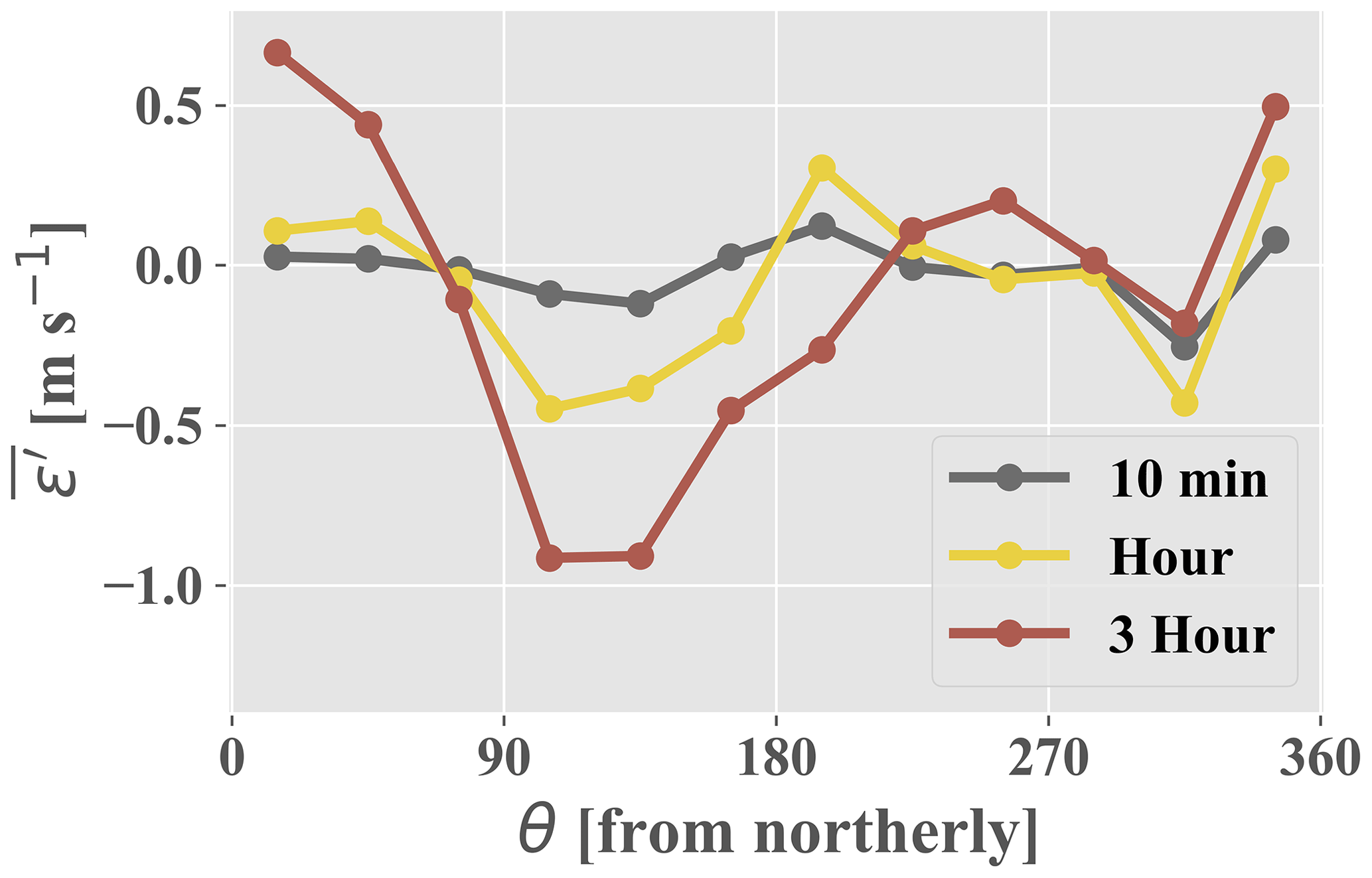
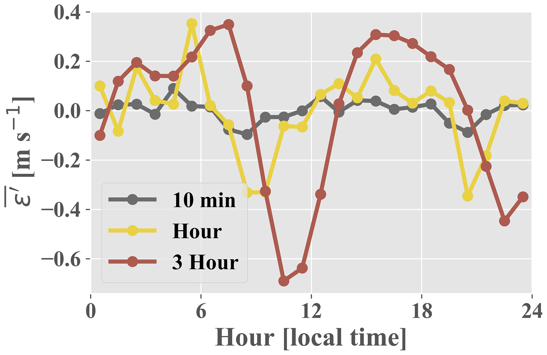
Table B1 The top row shows RMSE and MAE (both in m s⁻¹) obtained by the BCA. Below are the resulting RMSE and MAE values from ARIMA–RF predictions utilizing individual inputs for all forecasting timescales. Input features are separated into inertial (top), stability (middle), and turbulence (bottom) variables, as described in Sect. 4.