Surrogate-based aeroelastic design optimization of tip extensions on a modern 10 MW wind turbine

Advanced aeroelastically optimized tip extensions are among rotor innovation concepts which could contribute to the higher performance and lower cost of wind turbines. A novel design optimization framework for wind turbine blade tip extensions based on surrogate aeroelastic modeling is presented. An academic wind turbine is modeled in an aeroelastic code equipped with a near-wake aerodynamic module, and tip extensions with complex shapes are parametrized using 11 design variables. The design space is explored via full aeroelastic simulations in extreme turbulence, and a surrogate model is fitted to the data. Direct optimization is performed based on the surrogate model seeking to maximize the power of the retrofitted turbine within the ultimate load constraints. The presented optimized design achieves a load-neutral gain of up to 6 % in annual energy production. Its performance is further evaluated in detail by means of the near-wake model used for the generation of the surrogate model and compared with a higher-fidelity aerodynamic module comprising a hybrid filament-particle-mesh vortex method with a lifting-line implementation. A good agreement between the solvers is obtained at low turbulence levels, while differences in predicted power and flapwise blade root bending moment grow with increasing turbulence intensity.

1 Introduction

The trend of reducing the levelized cost of energy (LCOE) of horizontal axis wind turbines through increasing rotor size has long been established. To achieve this, the challenges of scale must be overcome through innovative turbine design and control strategies (Veers, 2019). One promising blade design concept is advanced aeroelastically optimized blade tip extensions, which could drive rotor upscaling in a modular and cost effective way.

The existing bibliography relevant to wind turbine applications typically focuses on winglets and aerodynamic tip shapes purely from an aerodynamics point of view (Johansen, 2006; Gaunaa, 2007; Ferrer, 2007; Chattot, 2009; Elfarra, 2014; Farhan, 2019; Matheswaran, 2019). Exceptions to this general trend are the recent articles (Zahle, 2018; Sessarego, 2018; Hansen, 2018; Rosemeier, 2020; Horcas, 2020) that put the focus on general blade tip designs and aeroelastic performance. Moreover, there is no relevant research work focusing on performance and design loads of rotors with tip extensions relevant to real operational cases with a view towards a business case. Only in Rosemeier (2020) is the potential of blade tip extensions for lifetime extension evaluated through aeroelastic fatigue load cases.

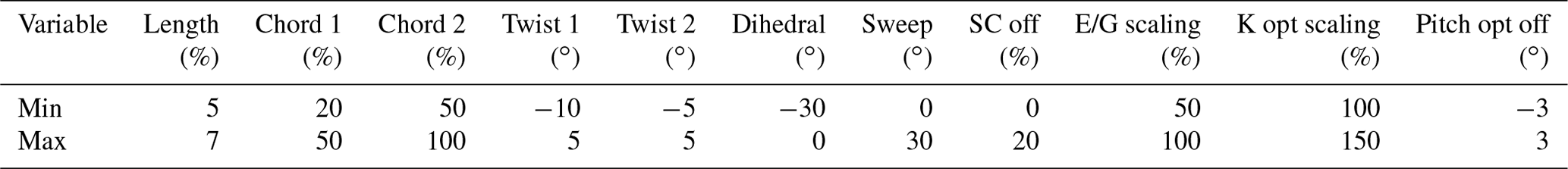
Table 1 Design variables and their range. Minimum (min) and maximum (max) values of planform design variables result in the “tip 1” and “tip 2” shapes shown in Fig. 1.

In this work, the tip extensions are designed with the objective of maximizing annual energy production (AEP) gain within the existing operational load constraints. The relevant business case is associated with improving the performance of existing rotors or customizing rotors for different site conditions while investing less in new full blade production costs. Due to the fact that full time-domain aeroelastic simulations are utilized for the power and load evaluation, a surrogate-based optimization (SBO) approach is pursued in order to avoid issues with gradient evaluations which normally require the simplification of the evaluation cases. Furthermore, the parametrization of the tip extension is detailed enough to represent a blade design optimization approach now in a modular way focusing only on the tip. This includes the capability of producing complex shapes with large sweep and prebend, which are typically not used in a traditional blade design.

2 Aeroelastic model setup

A time-domain aeroelastic model of the onshore version of the IEA 10 MW reference wind turbine (RWT) (Bortolotti, 2019) was first built. The IEA 10 MW RWT is an academic wind turbine model which is the result of aeroelastic optimization of the DTU 10 MW rotor. In particular the DTU 10 MW rotor was stretched in order to achieve the maximum AEP gain while satisfying the imposed design load constraints. The IEA 10 MW RWT design is considered a good representative reference of an optimized modern offshore wind turbine, for which the tip extensions could have a significant impact in the reduction of the LCOE.

A surrogate-based optimization framework was then wrapped around the baseline model of the IEA 10 MW RWT, with pre- and post-processing scripts providing the capability of executing simulations of specific tip extensions on the baseline turbine, with their design variables determined by the optimization routines.

The following sections provide further details of the different components involved in the above-described workflow.

2.1 Baseline model

The aeroelastic simulations performed in the present work relied on the commercial software HAWC2 (Larsen, 2007). HAWC2 includes advanced features in the near-wake (NW) aerodynamic module implementation, providing the ability to accurately simulate complex tip shapes (Pirrung, 2016, 2017; Li, 2018; Madsen, 2020). In addition to the modified near-wake model to account for blade sweep, the coupled aerodynamic module in HAWC2 uses a non-planar vortex cylinder model (Branlard, 2017) to compute the effects of prebend and out-of-plane deformation on axial- and radial-induced velocity.

The in-house multi-fidelity vortex solver MIRAS (Ramos, 2016, 2017) has been used for a higher-fidelity evaluation of the baseline and the optimized designs. In the present study the lifting line (LL) aerodynamic model is used in combination with a hybrid filament-particle-mesh flow model (Ramos, 2019). The flow is governed by the vorticity equation, which is obtained by taking the curl of the Navier–Stokes equation, and describes the evolution of the vorticity of a fluid particle as it moves with the flow. The coupling between MIRAS and HAWC2 (Ramos, 2020) permits us to account for the flexibility of the wind turbine, as well as the consideration of the effect of the controller and the hydrodynamic loads. MIRAS has been recently modified to accurately account for blade curvature effects (Li, 2020).

The power performance and ultimate loads of every design are evaluated in a single load case, comprising an IEC-specific DLC1.3 (IEC, 2005) simulation at 8 m s⁻¹. This case is considered representative for determining the average power performance in below-rated power operation and the range of peak loading since the turbine operation ranges from low power production to full-rated power within the simulation time. The 600 s extreme turbulence model (ETM) simulation ensures that a range of inflow and operating conditions is accounted for. Moreover, different turbulence intensities (TIs) are simulated in the last part of the article, together with full wind speed range power curves for the AEP evaluation. A full design load basis (DLB) would be preferable, but the load simulation cases have been kept to a minimum for a fast and robust optimization setup.

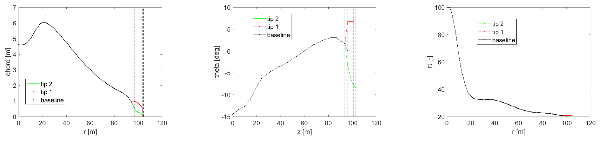
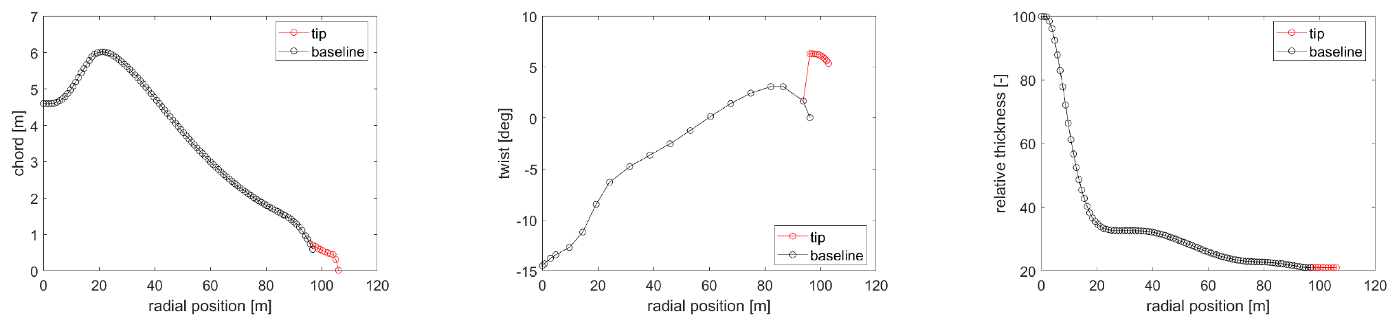
Figure 1 Planform for two reference tips at the borders of the design space. Vertical dashed lines indicate the location of the control points.

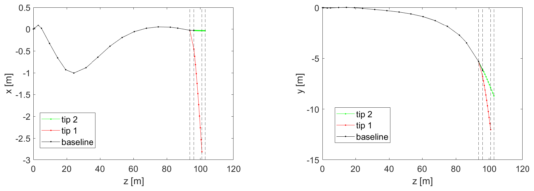
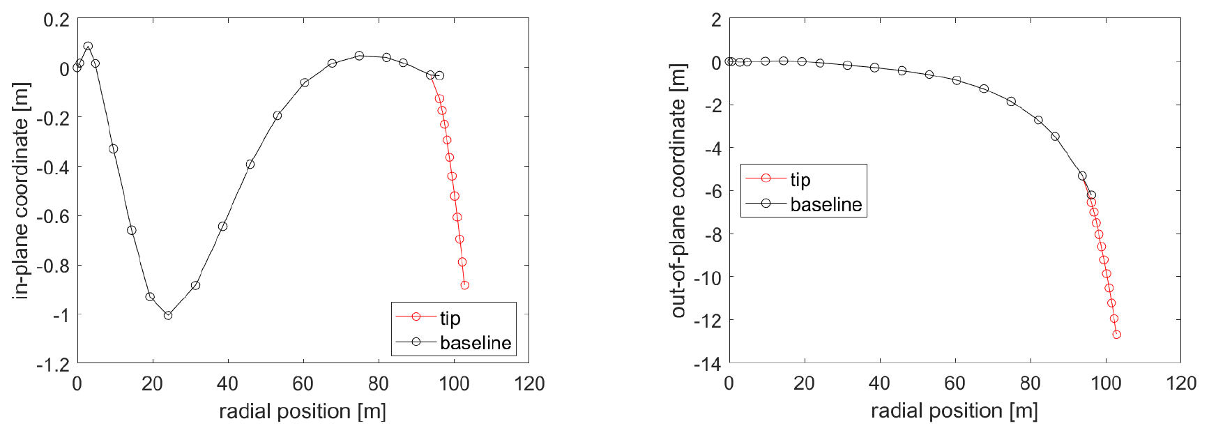
Figure 2 Blade centerline for two reference tips at the borders of the design space. Vertical dashed lines indicate the location of the control points.

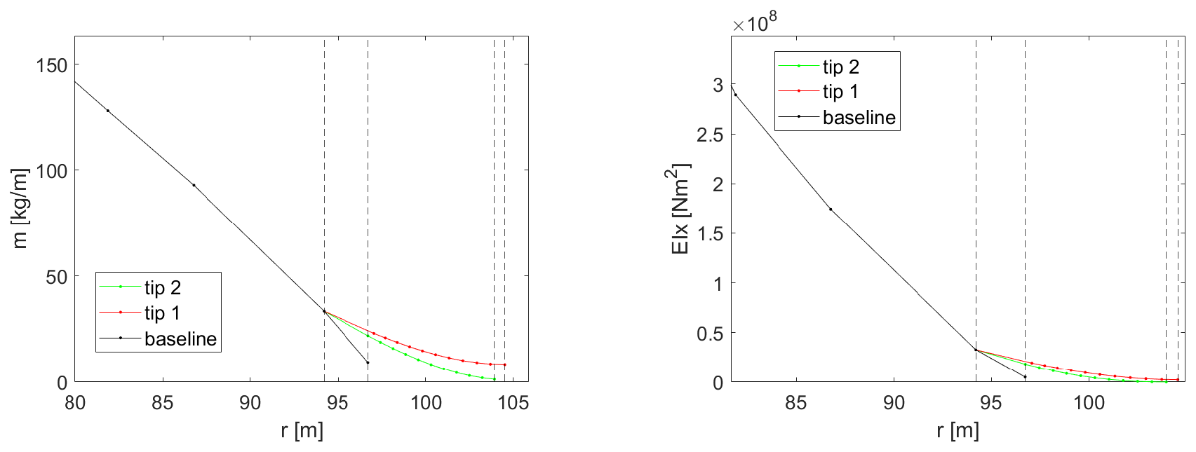
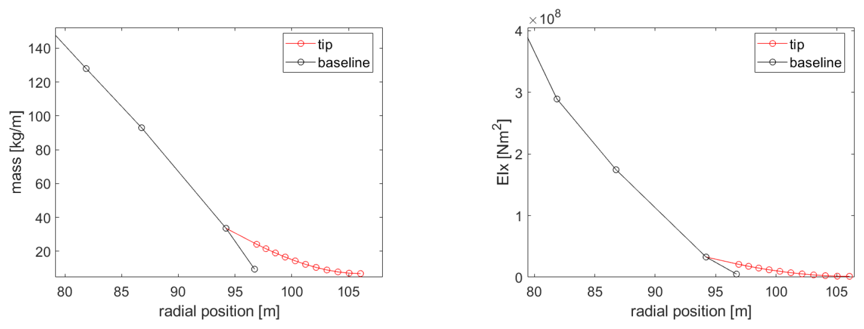
Figure 3 Mass and flapwise stiffness for two reference tips at the borders of the design space. Vertical dashed lines indicate the location of the control points.

2.2 Tip extension parametrization

The definition of the tip extension design variables and their design space is probably the most important step in the described optimization process. The variables have been chosen in a way which enables a general blade stretching design capability. Their range is a result of many prior parametric studies, and it is limited to ensure the validity of the aerodynamic modeling (Zahle, 2018; Li, 2018). The 11 chosen variables and their extent in the design space are shown in Table 1, with all definitions being relative to the baseline blade. When adding the extensions, the blade is cut at the connection point at 97.5 % of its original projected length in the spanwise coordinate, and the length of the extension is added. The tip extension planform is defined by the chord values at the new tip (chord 1) and the baseline tip (chord 2) positions and by the twist values at the new tip (twist 1) and the baseline tip (twist 2) positions, all relative to the values at the 97.5 % connection point. The relative thickness is defined by assuming the value at the new tip position is equal to the one at the baseline tip. The distribution of the planform variables is calculated with a cubic Hermite interpolating polynomial in order to have a smooth continuous shape extension from the baseline geometry with limited design variables. The planforms of two reference tip extensions at the borders of the design space are compared to the baseline one in Fig. 1. The same distribution approach is utilized for the angle of the section reference line, where a new tip in-plane (sweep) and out-of-plane (dihedral) angles are defined relative to the existing direction at the connection point. Only the backwards sweep and upwind offsets are modeled since there is no evident design benefit for forward sweep, and upwind dihedral results in a smooth shape continuation of the existing prebend further away from the tower. The offsets of two reference tip extensions at the borders of the design space are compared to the baseline one in Fig. 2 for a case of 30^∘ sweep and 30^∘ dihedral angles. The structural properties of the tip sections are calculated by scaling with the new chord values. Two variables are defined in order to vary the structural characteristics of the tip, accounting for moving the shear center position fore of the baseline position relative to the local chord (SC off) and scaling of the flapwise, edgewise, and torsional stiffness (E/G scaling). The mass and flapwise stiffness of two reference tip extensions at the borders of the design space are compared to the baseline one in Fig. 3. The main controller parameters changing with the tip addition account for the response in the below-rated operation by scaling the rpm-generator torque quadratic gain (K opt) and varying the fine pitch setting (pitch opt).

2.3 Pre- and post-processing

For every design evaluation loop, the HAWC2 case files are pre-processed, executed, and post-processed on a single CPU. The top-level process is shown in Fig. 4. In the pre-processing of the MATLAB script, the baseline HAWC2 input files are modified in order to generate each tip extension design case. In the HAWC2 model, 10 additional structural and aerodynamic sections are added on the new part of the blade beyond 100 %, and the sections between 97.5 %–100 % are modified. The rpm-generator torque quadratic controller gain and the fine-pitch setting are also modified. A case folder with all the HAWC2 input is assembled from all necessary files.

In the post-processing of the MATLAB script, the output time-series files of HAWC2 are processed, and performance statistics are extracted. For the optimization, the mean generator power and the ultimate blade root flapwise bending moment are extracted. For detailed evaluation purposes of the designs, all other component load statistics and blade-distributed outputs are also extracted.

Figure 4 SBO setup top-level diagram.

3 Surrogate-based optimization setup

The SBO framework is set up based on the MATLAB code package MATSuMoTo (Müller, 2013, 2014), which is the MATLAB Surrogate Model Toolbox for deterministic, computationally expensive black-box global optimization problems with continuous, integer, or mixed-integer variables that are formulated as minimization problems. The SBO framework determines the design variable sets and sends them to the pre-processor to execute the HAWC2 cases in parallel CPU processing. The general SBO algorithm works as follows.

• Generate initial design sets.

• Do the costly function evaluations at the points generated in the previous step.

• Fit a surrogate model to the data.

• Use the surrogate model to predict the objective function values at unsampled points in the variable domain to decide at which points to do the next expensive function evaluations.

• Do the expensive function evaluations at the points selected in the previous step.

• Check if the stopping criterion has been reached. If not, go back to the third step. If the stopping criterion has been met, stop.

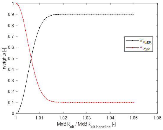
The objective function is a very important part of this study since it determines which direction in the design space the SBO takes by evaluating new design variable sets. The objective function is defined as a weighted sum of the mean generator power and the ultimate blade root flapwise bending moment. Since we do not pursue any purely load-alleviation-driven designs but load-neutral power-increase designs, the objective function is based only on the maximization of power when the loads are neutral or negative compared to the baseline. When the increase in loads is higher than 2 % (an empirical limit accounting for model uncertainty), the objective has a 90 % weight on loads and 10 % on power. A smooth Gaussian filter is used for the transition between neutral and higher loads (Fig. 5).

Figure 5 Power and load objective function weights as a function of load increase.

3.1 Surrogate modeling

For generating the initial sample set, MATLAB's Latin hypercube design is used with the maximin option and 20 iterations. The minimum sample size used is $\mathrm{3}\cdot d+\mathrm{1}$, where d is the number of design variables, in our case 11. In the initial set, a reduced cubic polynomial regression model is fitted. The choice of the surrogate model is decided based on prior studies of accuracy and comparing it with quadratic regression polynomials and radial basis functions. The chosen design of experiment (DOE) and surrogate model methods are based on the prior studies of Müller (2013, 2014), with the number of initial sample points in accordance to the model requirements and the chosen methods, given the fact that the focus of this work is not on the evaluation of the best optimization methods but on the evaluation of the potential design benefit of the chosen methods.

3.2 Optimization

Using the fitted surrogate model on the initial set, a global optimization approach is followed utilizing MATLAB's genetic algorithm with default settings. The best-performing design point is chosen for a HAWC2 evaluation, together with points created by randomly perturbing the best point found so far. In addition, a set of points that is uniformly selected from the whole variable domain is generated (using again a Latin hypercube design) and is added to the evaluation set. Hence, it is possible to improve the global fit of the surrogate model, and new areas of the variable domain where the global optimum may be located can be detected. Using 7 CPUs, 20 iterations are performed, resulting in a total of 174 HAWC2 evaluations, including the initial sample set of 34 points.

4 Results

The progress of the optimization and the results for the whole set of evaluated design samples is discussed here. The characteristics of the best converged design are also discussed in detail.

Table 2 Optimized design variables.

4.1 Optimization results

The progress plot showing the best value of the objective function during the evaluation of each sample is shown in Fig. 6. It is seen that the objective function value is improved considerably from the starting samples and practically converges after 140 evaluations. All evaluated samples are plotted in Fig. 7 in the state space of the two metrics, generator power and ultimate blade root flapwise bending moment, and are colored by the value of the objective function (weighted sum). A Pareto front is clearly visible with the best points laying on the front close to the zero load difference level. The optimal design point is designated by the red circle.

Figure 6 Progress plot of the objective function value.

Figure 7 Pareto front of the evaluated samples.

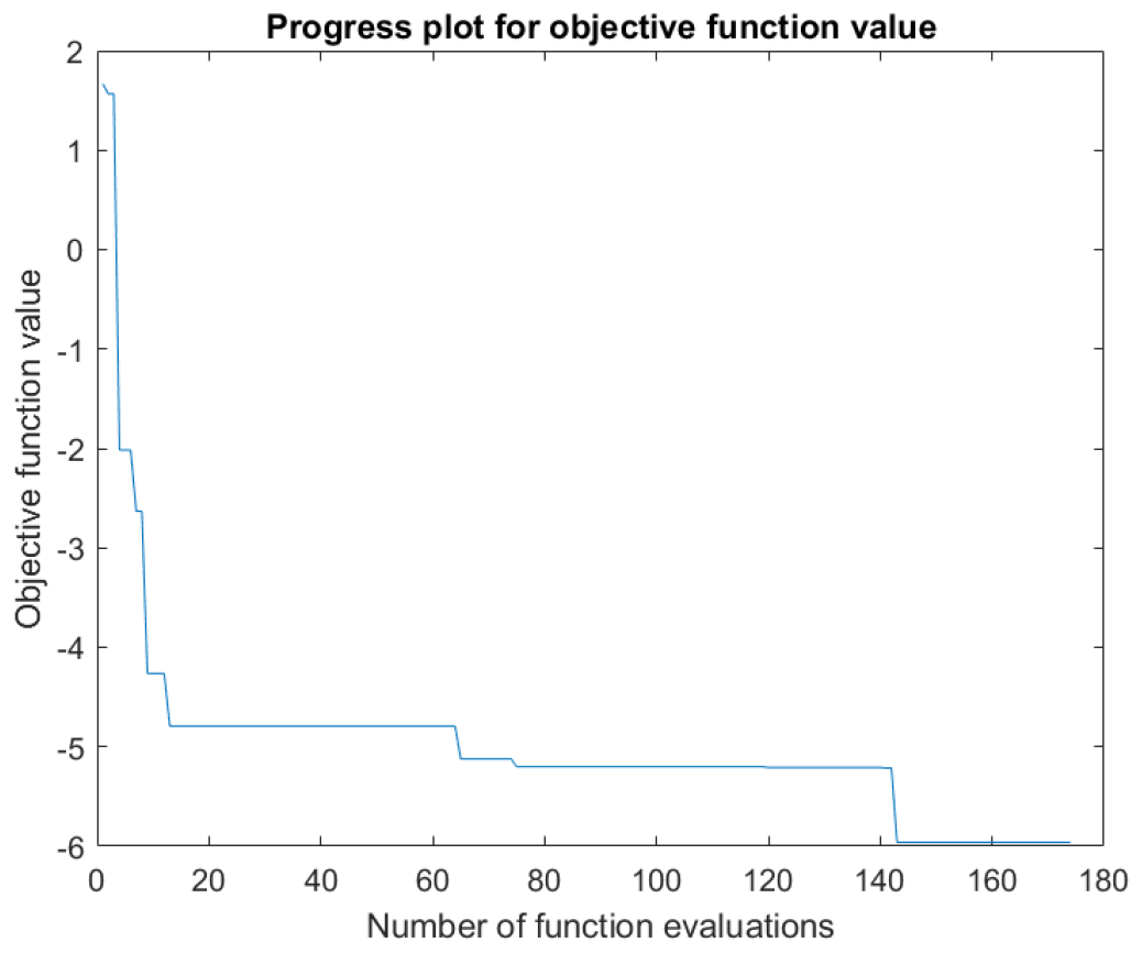
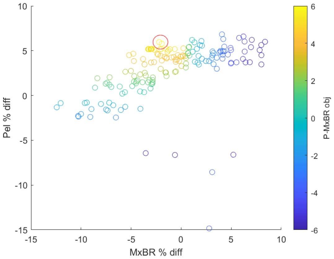
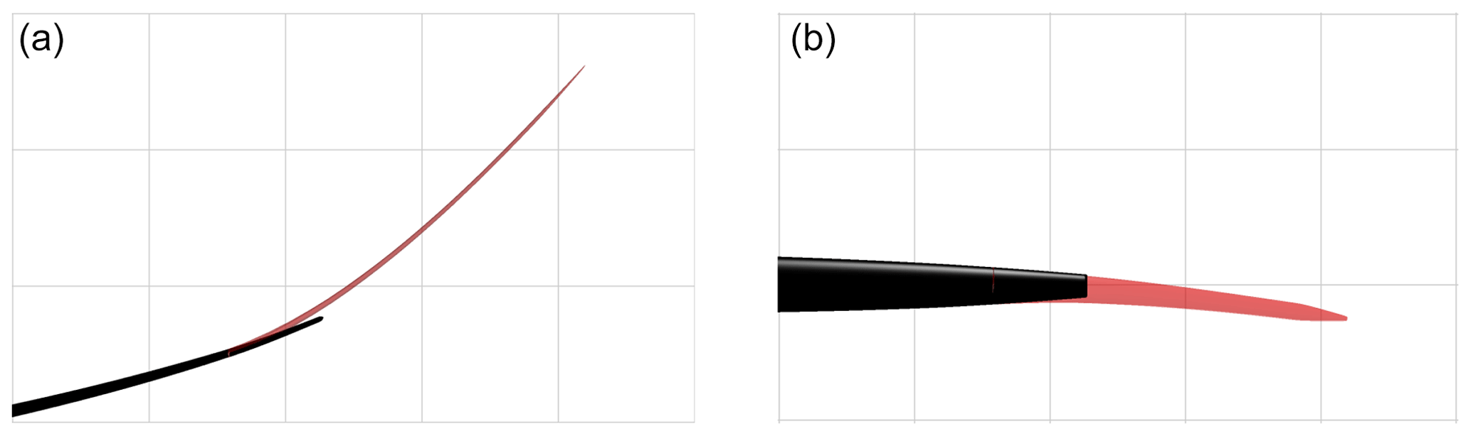
Figure 8 Blade 3D surface comparison between baseline geometry (in black) and optimized tip extension (in red). (a) In-plane view and (b) out-of-plane view. For reference, a background grid with a spacing of 3.5 m is included.

Figure 9 Blade centerline of the optimized design.

Figure 10 Planform of the optimized design.

Figure 11 Mass and flapwise stiffness of the optimized design (zoom-in of the tip).

The best design in terms of the minimum value of the objective function comprises a tip extension with a length close to the limit of the defined length (7 %), with all 11 design variables listed in Table 2. The design is shown to be a slender, backwards swept, and highly upwind prebent tip shape with fore positioning of the shear center, lower rotor speed, and higher pitch settings. In Fig. 8, the 3D geometry of the baseline and optimized blade tip is compared.

Table 3 Comparison of AEP predictions for the baseline and optimized designs between HAWC2-NW and HAWC2-MIRAS.

^a Relative to baseline – NW; ^b relative to baseline – MIRAS.

Figure 12 Power curve comparison between HAWC2-NW and HAWC2-MIRAS: (a) class I and (b) class III. Solid lines represent the baseline blade, while dashed lines represent the optimized tip design.

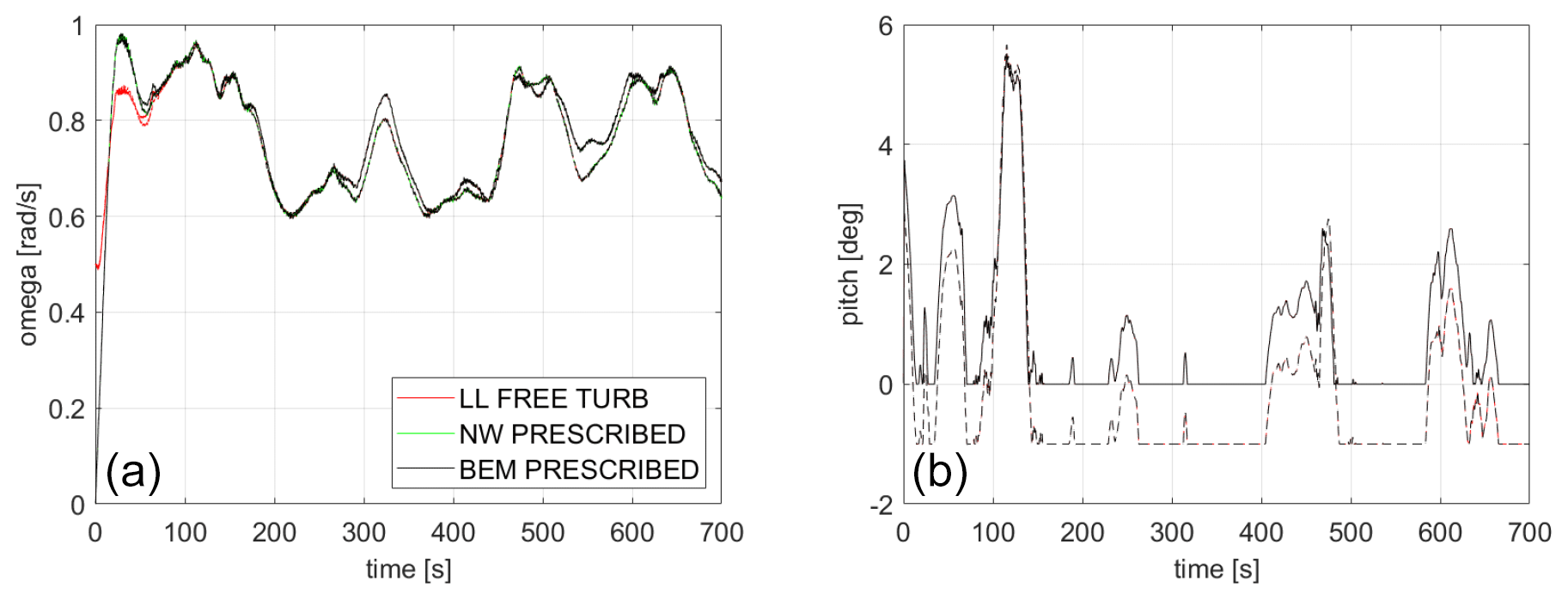
Figure 13 (a) Rotational speed and (b) pitch signal of the baseline and optimized design. Solid lines represent the baseline blade, while dashed lines represent the optimized tip design.

The blade centerline of the optimized design is compared to the baseline in Fig. 9, where the sweep and prebend offsets are shown. The optimized planform is compared to the baseline in Fig. 10. The mass and flapwise stiffness distributions are compared to the baseline in Fig. 11. The optimized distributions are generally smooth and realizable with the exception of the twist, which in a realistic application would have to be a smooth continuation of the maximum value of the baseline inboard of the tip.

Figure 14 Differences in power in the function of turbulence intensity (a) mean and (b) standard deviation. Solid lines represent the baseline blade, while dashed lines represent the optimized tip design.

4.2 Evaluation of optimized design

The performance of the optimized design is evaluated in terms of AEP in its IEC wind class I and the lowest average wind speed class III. The “clean” power curve is defined by steady uniform wind speed inflow from cut-in to cut-out with 1 m s⁻¹ steps and no wind shear or turbulence. The higher-fidelity aerodynamic module MIRAS is also used to run the same cases for comparison. The results are shown in Table 3, with the power curves plotted in Fig. 12. We see that MIRAS overpredicts the AEP of the baseline design by 1 % and underpredicts the AEP gain due to the tip by up to 2 %.

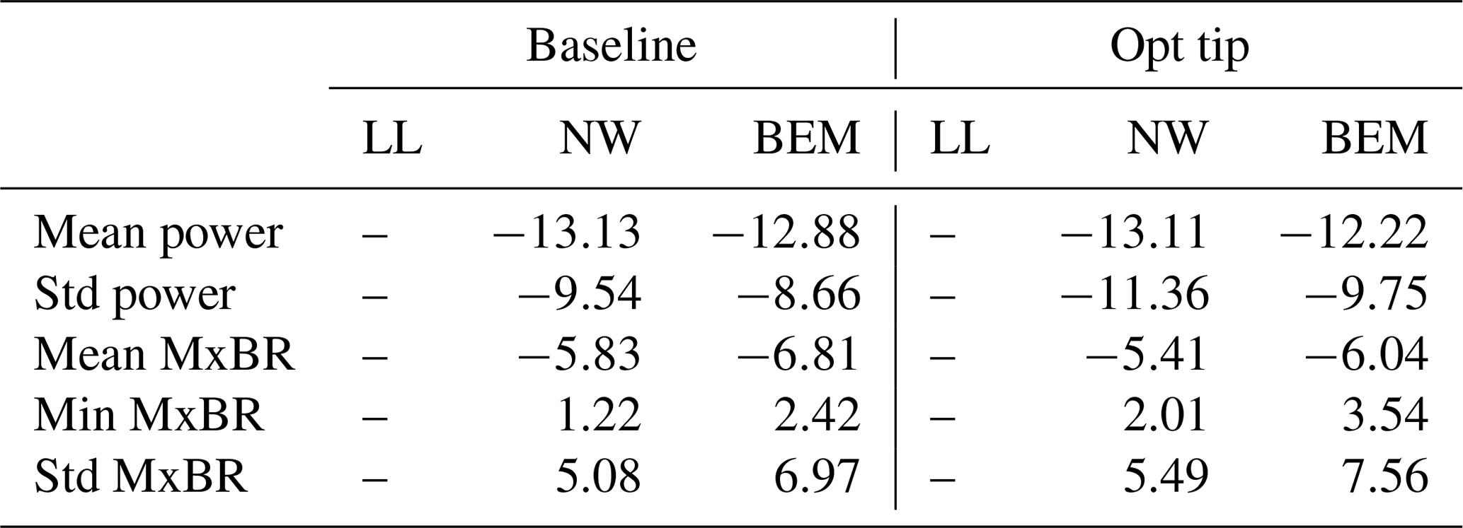
Table 4 Statistics of the power and flapwise root bending moment predicted in the extreme turbulence case by HAWC2-NW and HAWC2-BEM with respect to HAWC2-LL predictions. The table shows the difference in percentages.

The performance of the optimized design is also evaluated in the DLC1.3 (ETM) case which is used in the optimization and is performed with the NW method against two different fidelity models. The blade element momentum (BEM) model implemented in HAWC2 is used as the lower-fidelity method, and the lifting line aerodynamic module implemented in MIRAS is employed as the higher-fidelity solver. To ensure a meaningful comparison between the solvers, simulations of the extreme turbulent case have been carried out as follows. Firstly, to run a free turbulent simulation in MIRAS, the velocity-defined Mann turbulent box used in the optimization procedure has been transformed into a particle cloud by computing the curl of the velocity field. This cloud is slowly released one diameter upstream of the turbine, and it develops as it convects downstream towards the rotor plane. The released turbulent particles interact freely with the turbine wake. Vortex simulations with and without the turbine are performed. In the simulation without a turbine, the local velocities are extracted every time step at the rotor plane position in a 64×64 mesh with a cell size of approximately 6.25 m. These velocities differ from the initially defined turbulent box due to the downstream development of the flow in MIRAS. Such velocities are used to generate a new turbulent field which will be loaded in the HAWC2-NW and HAWC2-BEM simulations. Such a turbulent field will mimic the turbulence seen by the turbine in MIRAS, although the presence of the turbine and its wake will modify the turbulent field, and such phenomena can not be accounted for. In order to reduce uncertainties related to the turbine control in HAWC2, both the azimuthal rotor position and the pitch angle for each one of the blades are forced to be the same as the ones computed in the MIRAS simulation (with turbine), as shown in Fig. 13. In order to have a smooth start of the HAWC2-BEM and HAWC2-NW simulations, the first 60 s of the rotational speed signal from MIRAS has been modified using a hyperbolic tangent function. Differences between the simulations are therefore mainly related to the wake and flow modeling. The visible rotor speed differences (left plot of Fig. 13) appear between the baseline rotor and the rotor with optimized tip, and the different fidelity levels clearly operate at the same rotor speeds from 100 s simulated time. The pitch angles also agree well between fidelity levels. The main offset between the baseline and extended rotors is the minimum pitch angle that is reduced to 1^∘ (towards feather) by the optimization routine (see Table 2).

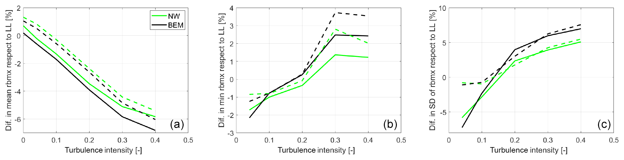
Figure 15 Differences in flapwise root bending moment in the function of turbulence intensity (a) mean, (b) minimum, and (c) standard deviation. Solid lines represent the baseline blade, while dashed lines represent the optimized tip design.

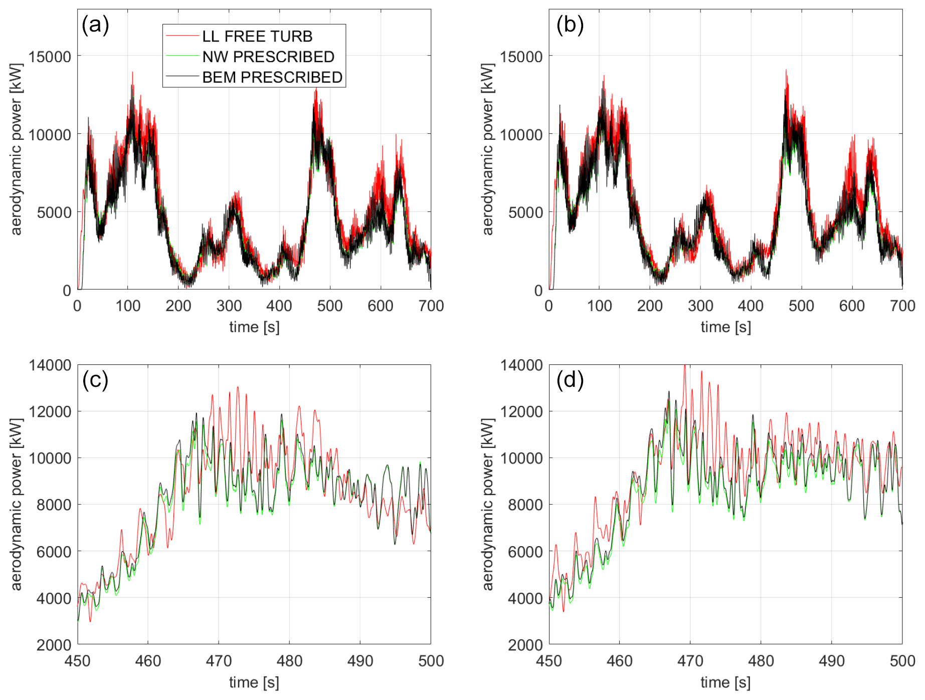
Figure 16 Aerodynamic power signal (a, c) baseline and (b, d) optimized design. (a, b) Full simulation time and (c, d) zoom-in for a 50 s time interval.

General statistics of the aerodynamic power and the flapwise root bending moment are presented in Table 4. Regarding the power, it seems like the BEM method is slightly closer to the LL predictions in both mean and standard deviations for both rotor designs. However, regarding the blade root flapwise moment (MxBR), the NW model is closer to the LL calculations for all quantities except for the minimum predicted value of the optimized blade. This is especially remarkable when looking at the standard deviation, in which the NW deviation from the LL simulations is 50 % smaller than BEM. Note here that the defined DLC 1.3 case has a turbulent intensity level of 40 %.

In order to study the influence of the turbulence level in the results, the extreme turbulence level of the DLC 1.3 (40 %) has been downscaled to obtain inflow fields with a range of turbulence intensities from 0 % to 40 %. Statistics of the difference in the BEM and NW predictions with respect to the LL simulations in the function of the turbulence level are presented in what follows. Figure 14 depicts the mean and standard deviation of the power signal. In terms of the mean, there is a clear increase in the differences respect to the LL simulations with the increasing turbulent intensity. The standard deviation of the power signal follows a different pattern with the smallest differences between the codes obtained for a TI of 20 %. An analysis of the mean, minimum, and standard deviation of the flapwise root bending moment signal is presented in Fig. 15. In this case, differences in the standard deviation of the signal are small for the optimized tip at low TIs and larger for the baseline; as the TI increases, the differences increase and align for both rotors. A similar picture is observed in the behavior of the minimum root bending moment values, although generally differences between the rotors increase with the TI. In terms of the mean values, differences with respect to the LL predictions grow with increasing TI, with the engineering models predicting a higher moment at low TI and a lower one at high TI.

A detailed analysis is carried out for the 40 % turbulent case. Figure 16 shows the time signal of the aerodynamic power for both blade designs with the three different fidelity models. Generally there is a good agreement between the three solutions. However, there is a small power offset in which the LL predictions are most of the time slightly larger than the BEM and NW predictions.

The time variation in the predicted flapwise root bending moment is shown in Fig. 17. Opposite to what is observed for the power signal, there is no clear offset between the LL and the NW/BEM model predictions. It is visible that the BEM calculations experience larger high-frequency variations compared to the higher-fidelity models, exhibiting a larger standard deviation as has previously been shown.

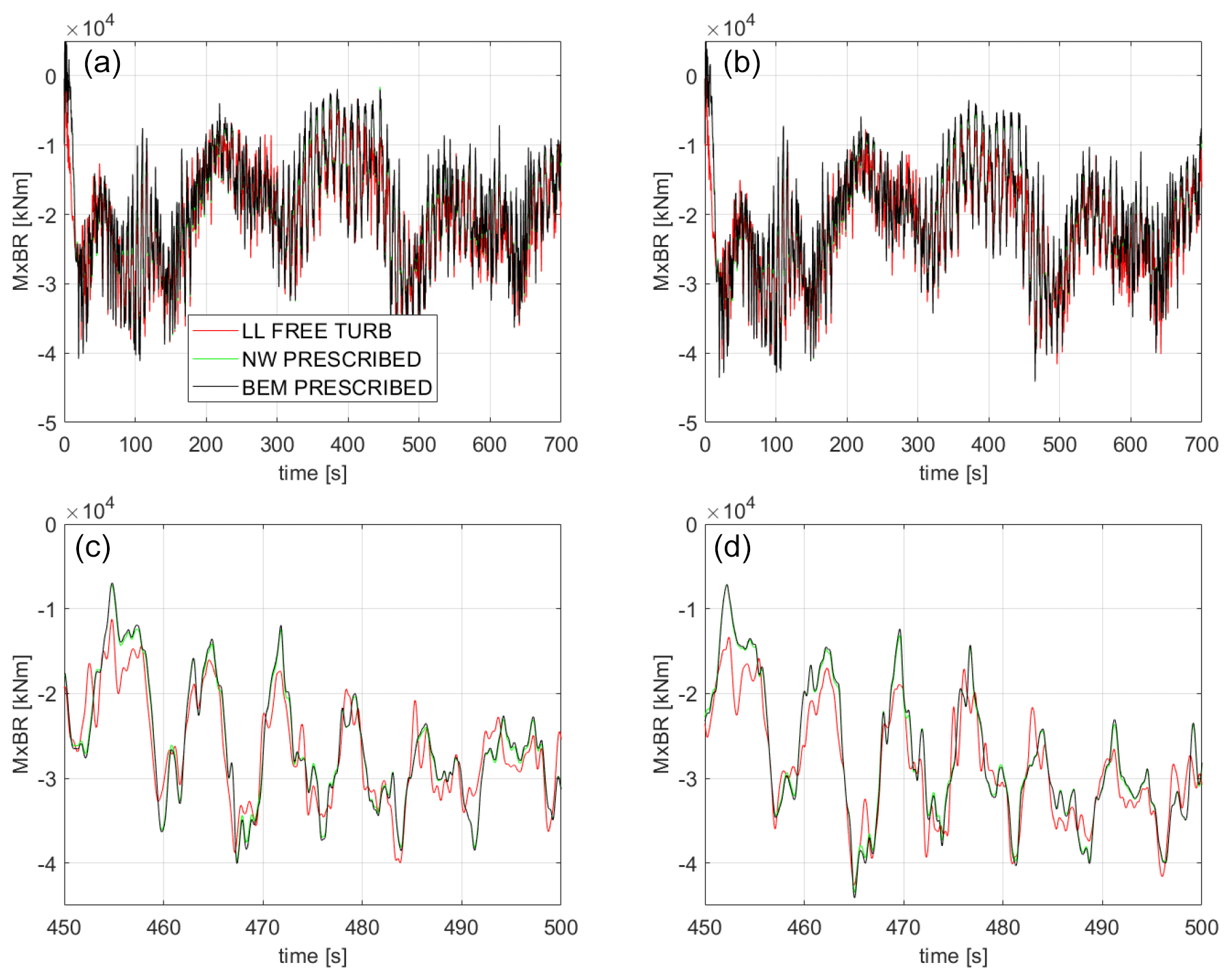
Figure 17 Flapwise root bending moment for MxBR (a, c) baseline and (b, d) optimized design. (a, b) Full simulation time and (c, d) zoom-in for a 50 s time interval.

The radial distributions of mean and standard deviation of area of attack (AOA) for the baseline blade (solid lines) and extended blade (dashed lines) are shown in Fig. 18. It can be seen that the mean AOA on the tip increases by roughly 4^∘ at the start of the tip extension, which is mainly due to the twist distribution (see Fig. 10). The MIRAS and the NW results both show decreased mean AOA inboard of the tip and an increased AOA on the tip itself. This is likely due to a load redistribution due to two factors: the offset of the trailed vorticity at the very blade tip and the velocity induced by the curved bound vorticity on the tip extension (Li, 2018). In the standard deviation of the AOA (right plot of Fig. 18), it can be seen that all codes predict the standard deviation to increase on the tip extension compared to the outboard part of the baseline blade. This is partly because the sweep angle reduces the fraction of the relative velocity that is in the planes of the aerodynamic sections, while it does not affect the wind speed changes due to turbulence. Thus the same turbulence will lead to larger variations in AOA on the swept-extended tip part of the blade than on the straight outboard part of the original blade. It can also be seen in all fidelity levels that the AOA is varying less on the section between 80 and 95 m radius on the extended blade than on the original blade, which is due to the aeroelastic load alleviation effect that the swept tip provides. The higher mean and standard deviation of the AOA inboard of 80 m radius on the extended blade is due to the reduced minimum pitch angle and due to the slightly reduced rotor speed (see Fig. 13).

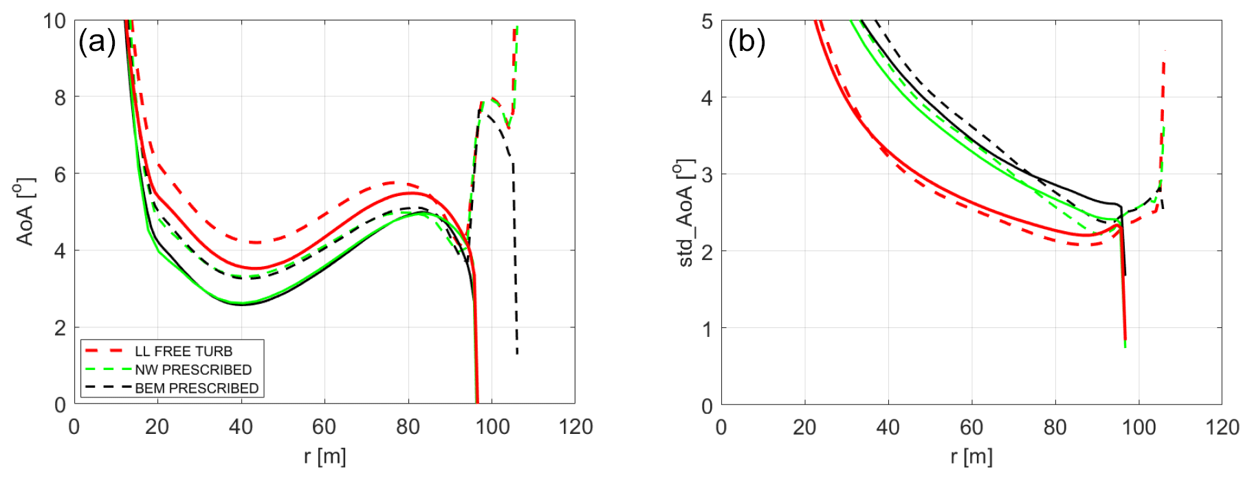
Figure 18 Angle of attack (a) mean distribution and (b) standard deviation. Solid lines represent the baseline blade, while dashed lines represent the optimized tip design.

The mean and standard deviation of the in-plane force are shown in Fig. 19. The overprediction of the mean in-plane force in the LL simulations corresponds to the mean power overprediction shown in Table 4. Again the load redistribution on the swept tip can be seen clearly, with increasing loads on the tip itself and decreasing loads inboard of the tip predicted by the LL and NW models compared to the BEM code prediction. All codes predict very similar standard deviations of the in-plane force.

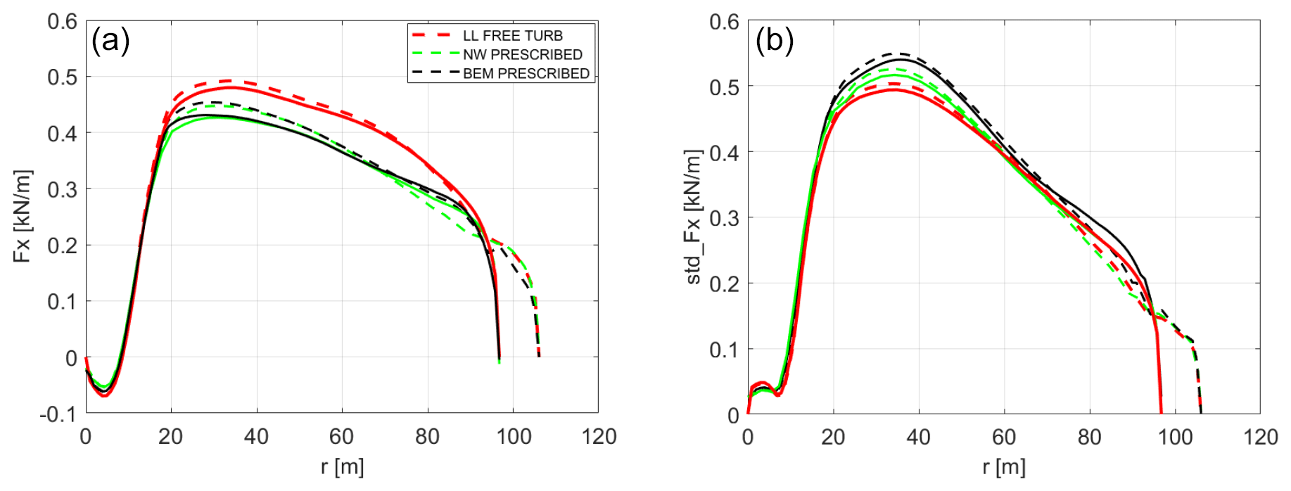
Figure 19 In-plane force (a) mean distribution and (b) standard deviation. Solid lines represent the baseline blade, while dashed lines represent the optimized tip design.

Similar effects can be seen in the out-of-plane forces in Fig. 20. The standard deviation of the NW computations is consistently below the BEM predictions, which is in good agreement with the comparisons in (Madsen, 2018). The aeroelastic load alleviation due to the geometric bend–twist coupling caused by the swept tip is clearly visible inboard of the tip section down to a radius of 50 m. In that part of the blade, all three codes predict lower load variations for the extended blade than the baseline blade. The fact that the BEM computations agree very well with the higher-fidelity codes on this load reduction indicates that it is an aeroelastic effect.

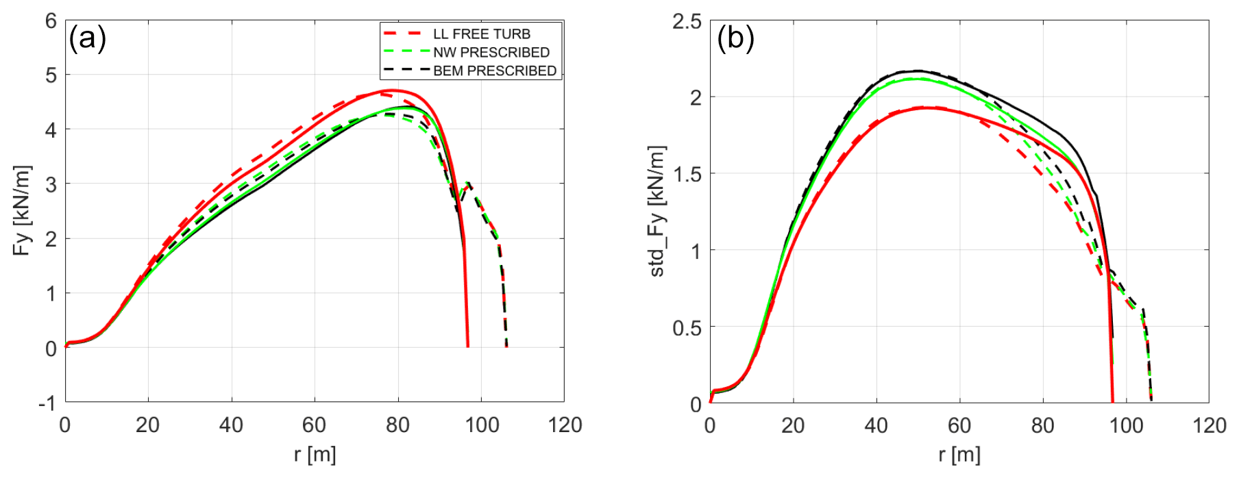
Figure 20 Out-of-plane force (a) mean distribution and (b) standard deviation. Solid lines represent the baseline blade, while dashed lines represent the optimized tip design.

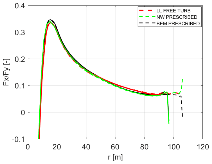
Figure 21 Mean values of the aerodynamic efficiency, $Fx/Fy$. Solid lines represent the baseline blade, while dashed lines represent the optimized tip design.

5 Conclusions

A novel surrogate-based optimization framework for aeroelastic design of tip extensions on modern wind turbines is presented in this work. The design of tip extensions is performed in a realistic design space and aeroelastic operation of the wind turbine, and it is highly efficient in terms of the use of computational resources. The optimized design achieving load-neutral 6 % AEP gain is evaluated in detail with two levels of aerodynamic model fidelity. The aeroelastic response predictions of the complex tip shape with the near-wake aerodynamic module agree fairly well with the higher-fidelity MIRAS simulations. A detailed comparison including a BEM model shows that local load distributions are predicted better by the near-wake model, but the improvement in terms of mean power and blade root loading over the BEM model is not clear. This indicates that the coupling factor computation in the near-wake model should be revisited. The agreement between the lower-fidelity BEM model, the near-wake model, and the higher-fidelity MIRAS model worsens with increasing turbulence intensity, which should be investigated in more detail in future work. The tip extension design concept resulting from the SBO process has high potential in terms of actual implementation in a real rotor upscaling with a potential business case in reducing the LCOE of future large wind turbine rotors. Future work will focus on introducing multi-fidelity optimization methods but also concept innovations which could further increase the achieved performance potential.