Understanding and mitigating the impact of data gaps on offshore wind resource estimates

Like almost all measurement datasets, wind energy siting data are subject to data gaps that can for instance originate from a failure of the measurement devices or data loggers. This is in particular true for offshore wind energy sites where the harsh climate can restrict the accessibility of the measurement platform, which can also lead to much longer gaps than onshore. In this study, we investigate the impact of data gaps, in terms of a bias in the estimation of siting parameters and its mitigation by correlation and filling with mesoscale model data. Investigations are performed for three offshore sites in Europe, considering 2 years of parallel measurement data at the sites, and based on typical wind energy siting statistics. We find a mitigation of the data gaps' impact, i.e. a reduction of the observed biases, by a factor of 10 on mean wind speed, direction and Weibull scale parameter and a factor of 3 on Weibull shape parameter. With increasing gap length, the gaps' impact increases linearly for the overall measurement period while this behaviour is more complex when investigated in terms of seasons. This considerable reduction of the impact of the gaps found for the statistics of the measurement time series almost vanishes when considering long-term corrected data, for which we refer to 30 years of reanalysis data.

1 Introduction

A wind resource assessment is performed at the beginning of every wind energy project. The wind resource is estimated for the site that is pre-selected with respect to the expected lifetime of the project, i.e. for the 20–30 years in the future during which the wind turbines will be operated at the site (Rohrig et al., 2019). During the lifetime of a wind farm, re-assessments are also typically done that can be based on wind turbine or further wind measurement data. Based on this estimate, an expected energy yield is derived which serves as a basis for any economic considerations of the project. Consequently, uncertainties and a possible bias in the wind resource estimate propagate up to the financing of a wind project with the percentage uncertainty value increasing from uncertainty in wind speed to uncertainty in wind farm production to uncertainty in the expected return on investment. Thus, to reduce these uncertainties, starting from the wind measurements is of high interest and relevance.

A wind resource assessment is typically based on a short-term measurement on site, which is conducted several years prior to the installation of the wind farm and has a duration on the order of a year (MEASNET, 2016; FGW e.V., 2017). The campaign duration is in most cases a compromise between informative value – defined by the representativeness of the measurements for the lifetime of the wind farm, i.e. those 20–30 years in the future – and the costs of the measurement campaign. In a later step, short-term measurements are long-term extrapolated making use of a reference dataset that is either a longer multi-year measurement in the surrounding area of the site or data from a reanalysis, sometimes downscaled with the use of a mesoscale model, with a resolution of several (tens of) kilometres around the site (Carta et al., 2013). In the case of complex terrain or differing measurement heights, horizontal and vertical interpolation is done using numerical computational fluid dynamics (CFD) and/or simplified engineering models (Rohrig et al., 2019).

Almost all measured time series have data gaps due to failures of the sensors themselves, a data logger or the power supply or due to adverse conditions such as a low aerosol concentration or unwanted fixed echoes for remote sensing devices (MEASNET, 2016). In case of offshore measurements, data gaps often further increase due to limited accessibility to the measurement installation in particular in high wind and wave conditions that may typically last for several weeks or even prevent access for a whole season. Additionally, many offshore wind measurements are not fully redundant due to their high costs, which is particularly the case for many floating lidar applications that prevail more and more in the offshore wind industry as a most cost-efficient alternative to fixed offshore meteorological (met) masts (Gottschall et al., 2017).

Up to a certain threshold of frequency and length of data gaps, the long-term extrapolation, which in the standard procedures involves some correlation of measured and reference data for the overlapping period, is often applied to the not fully continuous time series. MEASNET (2016), for instance, considers a measurement to be incomplete only when the availability of filtered data is less than 90 %. As an alternative, the time series can be “filled” before the application of the correlation analysis. Gap-filling procedures typically use reanalysis data, e.g. from MERRA2 (Donlon et al., 2012) or ERA5 (Hersbach and Dick, 2016), often downscaled with a mesoscale model such as WRF (Skamarock et al., 2019). Such a gap filling is, in particular, applied when the gap corresponds to a substantial discontinuity in a measurement time series of several days, weeks or even months, not just a few data points that can be filled by statistical approaches or even interpolation only.

Gap filling is a task that is not specific to the wind resource assessment application but can be of relevance for any measured time series or collected dataset where data gaps may significantly impact the outcome of the following data analysis. In the most general context, procedures to compensate for missing values in a dataset are referred to as imputation. There are a number of different imputation procedures that have in common that missing data are not simply ignored but instead replaced by plausible values. Specific gap-filling procedures for meteorological time series are discussed in Körner et al. (2018), Pappas et al. (2014) and the references herein, for example. These procedures include

• linear interpolation from adjacent time steps (particularly for cases where only a few data points are missing);

• autoregressive models (for longer periods of missing data and without adjacent sites as possible predictors);

• different methods of spatial interpolation (in case adjacent sites are available);

• data-driven methods like nearest-neighbour approaches, linear or multiple linear regression, look-up tables, or artificial neural networks (Körner et al., 2018).

For the wind resource assessment application, linear regression methods are of particular interest since they are often already used for the long-term extrapolation in the context of measure–correlate–predict (MCP) approaches (MEASNET, 2016). Often further dimensions are introduced by considering separate wind direction sectors or wind speed bins. Generally, MCP methods are not limited to linear regressions (see Carta et al., 2013, for a broader overview); however, in practice they are most often implemented in this way. This is why we concentrate on this type of procedure – both for data gap filling and long-term extrapolation – in this contribution.

The overall scope of the study is as follows: before discussing a selected specific data gap-filling approach, we investigate how data gaps impact the standard wind resource estimates by deriving and evaluating bias and uncertainty measures for wind time series with artificial gaps of varying length and seasonal period of occurrence. We repeat this analysis for the time series where the gaps are filled and, with this, study to which extent the impact of the gaps can be mitigated. The study is applied to the statistics of the short-term dataset, defined by the period of the measurements, as well as to the final long-term estimate, since both sets of results are relevant in the wind energy context. By deriving and comparing conclusions for three different offshore sites – in the German Bight, the Dutch North Sea and in the Baltic Sea – we also address the impact of the site and possible dependencies.

The article is structured as follows: in Sect. 2 we describe the data basis and in Sect. 3 the methods for this study. Section 4 presents the results for the impact of ignored and filled gaps on the short-term and long-term wind statistics. In Sect. 5 we discuss our findings with the particular implications for future resource assessment studies. And, finally, in Sect. 6 we summarise the main conclusions of our study.

2 Data basis

The data basis consists of measurement data from met masts over a measuring time which is characterised by a high availability on the basis of which the influence of measurement gaps and their filling is investigated (Sect. 2.1), as well as numerical data used for filling the gaps in the measurement data and the subsequent long-term extrapolation (Sect. 2.2).

2.1 Sites and measurement data

The analyses in this study are done independently for three different offshore met masts representing different typical sites for offshore wind energy utilisation in Europe. Two masts are located in the North Sea (FINO3 and IJmuiden) both about 50 km offshore from the nearest coastline with large wind direction sectors where the nearest coastline is several hundreds of kilometres upstream. The third mast (FINO2) is located in the central southern Baltic Sea and surrounded by land within 50 km or less except for a small wind direction sector. The sites were chosen to represent typical European offshore wind exploration areas with different distances to the coasts and varying atmospheric stability (see e.g. Dörenkämper, 2015; Kalverla et al., 2019).

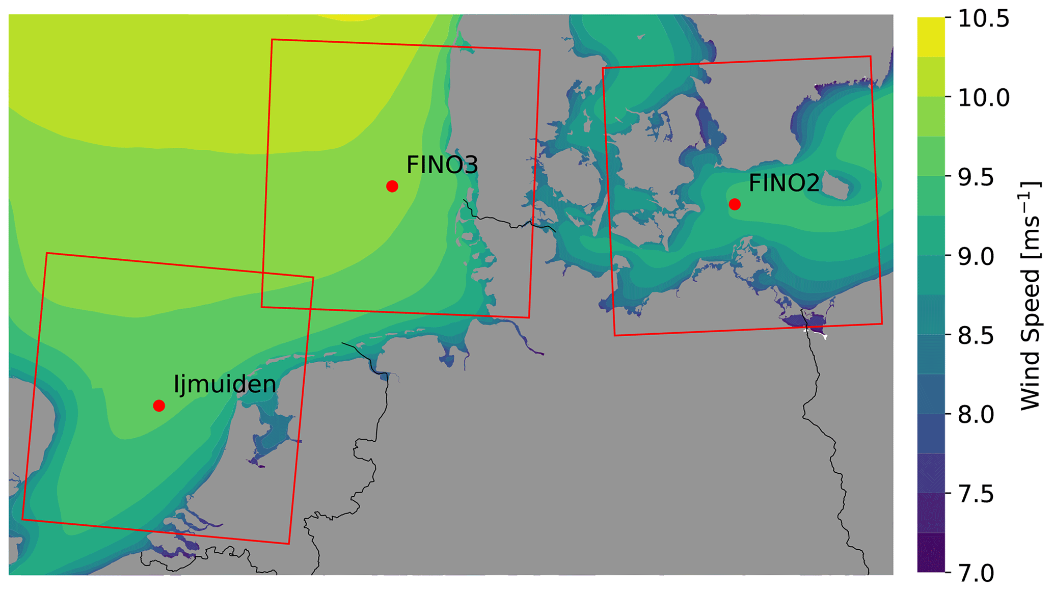
Figure 1 Position of the three sites (met masts) investigated in the framework of this study. The red boxes mark the sizes of the innermost domains used for the mesoscale modelling (see 2.2). The background wind field represents the 30-year mean wind speed (1989–2018) at 100 m height above the sea surface taken from the New European Wind Atlas (Hahmann et al., 2020; Dörenkämper et al., 2020). The coastline and border data originate from the GSHHS dataset (Wessel and Smith, 1996).

In Fig. 1 the positions of the three met masts are given. The frames mark the area of the innermost domains of the mesoscale data used for the gap filling (see Sect. 2.2). The data of all three met masts are freely available for scientific purposes. All of the masts are equipped with cup or sonic anemometers and wind vanes up to a height of 100 m above the sea surface. For our study we consider the 10 min averages of horizontal wind speed and direction data provided by these sensors. A measurement height close to 90 m was chosen at all three masts (see description below for more details), representing a typical hub height of offshore wind turbines. The 24-month period from 1 July 2012 to 30 June 2014 was selected based on the combined data availability for all three masts and other constraints such as limiting disturbance of wakes of nearby wind farms that were erected afterwards in the vicinity of the masts some years after the commission of the respective masts.

As the aim of this study is to investigate the impact of gaps on offshore wind-energy-relevant wind statistics, a reference time series with a low amount of missing data was needed. Thus, besides the selection of the 2-year period with a low number of gaps, further gaps were filled with measurement data from lower altitudes. To consider the wind speed dependence with height, a speed-up factor (sup) is defined according to $\text{sup}=\text{WS}{\mathrm{90}}_{\text{mean}}/\text{WS}[X{]}_{\text{mean}}$, where WS90_mean is the average wind speed at the measurement altitude of the mast closest to 90 m and WS[X]_mean the average wind speed of the measurement at a lower height and applied to the wind speed measurement of the lower altitude. In the case of gaps, the wind direction measurements were filled by measurements at lower heights as well but without using any scaling or offset correction. Data gaps in the mast measurements filled by applying this pre-processing are shown in Fig. 2. A short description of the three met masts with references to more detailed information is given in the following.

• The IJmuiden met mast¹ is located about 85 km west of Den Helder in the Dutch part of the North Sea. The met mast was in operation between November 2011 and March 2016 and was decommissioned afterwards. The mast was used in several wind energy research studies (e.g. Baas et al., 2016; Kalverla et al., 2019). It provides measurements at several heights and is described in more detail in Poveda et al. (2015). For the analysis in this study, the mast-corrected wind speed measurement (cup anemometers) located at 92 m height was used together with the wind direction measurement at a height of 87 m. The availability of the wind speed measurement data at these heights is 99.5 % prior to and 99.7 % after the filling of gaps by lower measurement heights (see procedure above).

• The FINO2 met mast² is located in the central southern Baltic Sea close to the border triangle of Denmark, Germany and Sweden in the German part of the Baltic Sea. In contrast to the North Sea sites, the FINO2 measurements are affected by the surrounding lands with distances of less than 50 km for the majority of wind direction sectors. Only a narrow northeasterly sector is dominated by a long marine fetch. FINO2 has been in operation since August 2007, and the data were studied in several wind-energy-related studies (e.g. Gryning et al., 2014; Dörenkämper, 2015). FINO2 provides wind measurements at various heights between 32 and 102 m a.s.l., technically described in FINO2 (2007). In this study mainly the wind speed measurements from the cup anemometers at 92 m height were used in combination with the wind direction measurement (vane) at the same height on the boom of the opposite side of the mast. The availability of the wind speed time series was 86.4 % prior to and 95.5 % after the application of the gap filling from lower heights (see procedure above).

• FINO3 is a met mast³ located in the northern part of the German Bight about 80 km northwest of the island of Sylt. Thus, the impact of upstream coastlines is very limited and a pure offshore climate is found in particular for the main wind direction sectors (south to northwest). FINO3 has been in operation since September 2009 and provides wind measurements each 10 m between 32 and 102 m a.s.l. as described in FINO3 (2012). The FINO3 wind measurements were part of several wind energy studies (Peña et al., 2015; Gryning et al., 2016). This study analyses the wind speed (cup) and wind direction (vane) data from the measurements at 92 m and 101 m a.m.s.l. These wind speed measurement data have an availability of 98.4 % prior to and 98.9 % after the application of gap filling from measurements at lower heights (see procedure above). A detailed overview of the measurements of the three FINO masts, their device types, accuracy and boom orientations is given in the Appendix of Leiding et al. (2012). Less than a kilometre west of the FINO3 platform, the wind farm DanTysk was constructed between February 2013 and April 2015. The erection of turbines did not start before April 2014, and operation did not start before December 2014. So, the wind statistics of FINO3 considered for this study should not be impacted by wakes of DanTysk.

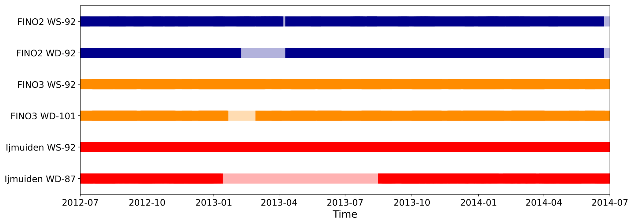
Figure 2 Data availability at the three masts after filling in the pre-processing step. The light colours indicate values that were filled by measurements from lower heights as described above.

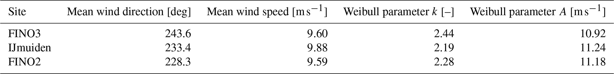
Wind speed and wind direction distributions for the three datasets of measurements are shown in Fig. 3. Note that the measurement heights slightly differ for the three sites – as described above, wind speed measurements are recorded at 92 m on all three masts, while wind directions are recorded at 87 m (IJmuiden), 92 m (FINO2) and 101 m (FINO3). Derived wind statistics are summarised in Table 1. Here and for the following analysis we consider the parameters mean wind direction and mean wind speed and the parameters k (Weibull shape parameter) and A (Weibull scale parameter) that are obtained from fitting a Weibull distribution function to the wind speed distributions. The fitting procedure is implemented as a nonlinear least-squares regression considering the complete wind speed range. All three masts represent typical midlatitude offshore wind climates. A shift from southwesterly to more westerly winds is found while moving from west to east, being in line with the typical track of cyclones when moving across central Europe (van Bebber, 1891).

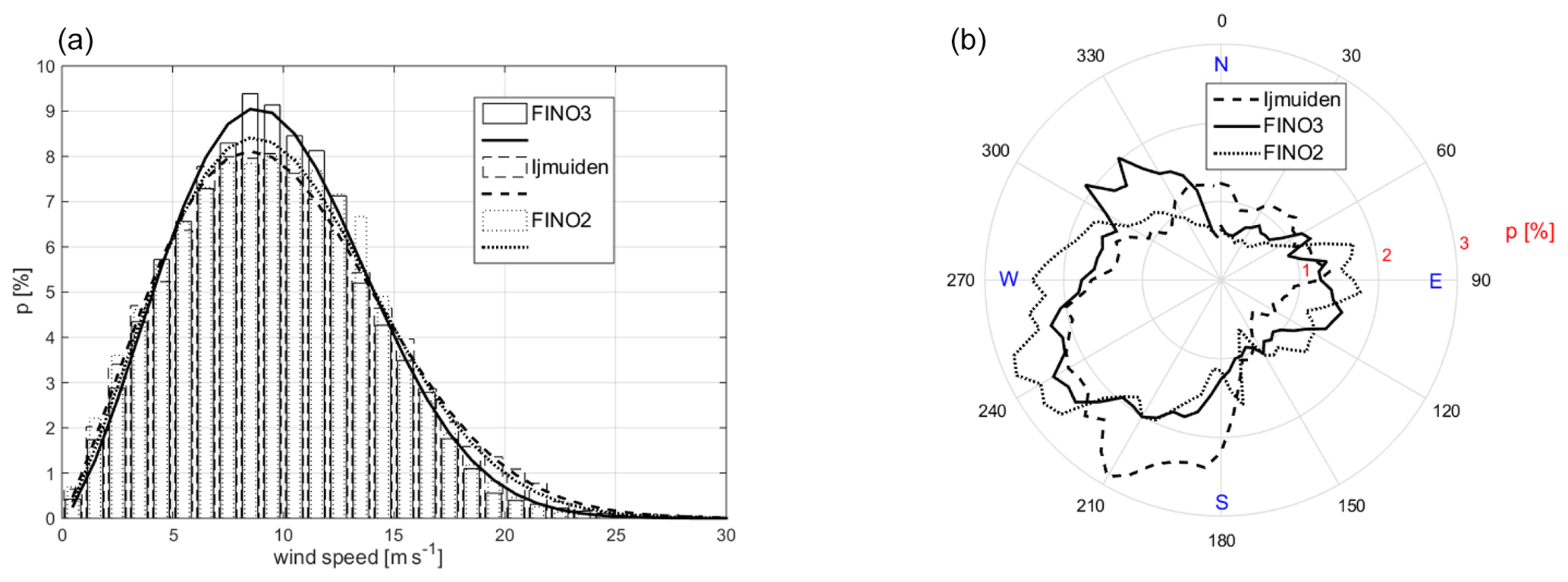
Figure 3 Wind speed (a) and wind direction (b) distributions for the three 24-month datasets from the FINO3, IJmuiden and FINO2 offshore met mast sites. Derived statistics are summarised in Table 1.

Table 1 Derived statistics for wind direction and wind speed distributions for the three datasets of site measurements.

2.2 Numerical data for gap filling and long-term extrapolation

The procedures applied for this study make use of regional mesoscale modelling data that are used for the gap filling, as well as long-term reanalysis data that are applied for long-term referencing of the wind measurements. These data sources are described separately below.

2.2.1 Reanalysis data

For the long-term extrapolation, the data from the ERA5 reanalysis (Hersbach et al., 2020) were used. ERA5 is the most recent generation of reanalysis data issued by the European Centre for Medium-Range Weather Forecasts (ECMWF) since 2017. For wind energy applications it was shown to outperform other reanalyses (e.g. Olauson, 2018; Thøgersen et al., 2017). ERA5 provides reanalyses on all important atmospheric and oceanographic parameters at an hourly resolution in time and 0.25^∘ (≈30 km for the atmospheric parameters; others differ) in zonal and meridional directions globally. Currently the period of 1979–ongoing is publicly available with a lag of a few days in time. For the long-term referencing in this study, the wind speed (zonal and meridional components, u and v at 100 m) from the so-called surface-level data of the ERA5 dataset were selected for the period 1983–2014 to cover a climatic period of 30 years. Most recently, mesoscale model datasets with a higher resolution on the order of a few kilometres were made available for longer periods (up to 30 years) and sometimes used for long-term referencing. However, as the industry at least partly still relies on classical lower-resolution reanalyses, we have applied this approach for our study. In addition, due to its comparatively high resolution ERA5 does not show major differences in the offshore wind speed climate statistics several tens of kilometres away from the coastal discontinuity (Dörenkämper et al., 2020).

2.2.2 Mesoscale modelling and data

The mesoscale model data in this study are used for filling the gaps that are artificially cut into the time series. In principle any mesoscale model data could be used, such as those from the publicly available New European Wind Atlas (NEWA) (Hahmann et al., 2020; Dörenkämper et al., 2020) or commercial products. However, these data are often not optimised for offshore wind energy applications or only available in lower resolution in time (e.g. 30 min instead of the desired 10 min data). Consequently, simulations were performed separately for this study, applying a setup that was optimised for offshore wind applications (Dörenkämper et al., 2015, 2017; Gottschall et al., 2018) and capable of resolving the most important flow features in offshore development regions.

The simulations were carried out using the Weather Research and Forecasting (WRF) model (Skamarock et al., 2019) in its version 4.0.1, which is generally well known and commonly used in the wind energy community (e.g. Dörenkämper et al., 2015; Hahmann et al., 2020). The mesoscale simulation setup was similar for all three sites, consisting of three domains with resolutions of 18, 6 and 2 km and a domain size of 150×150 GP (grid points) for each domain, centred around the site of interest (i.e. the respective offshore met mast). Figure 4 exemplarily shows the size of the three domains for the FINO3 site. The sizes of the innermost domains (D3) for all three sites are given in Fig. 1.

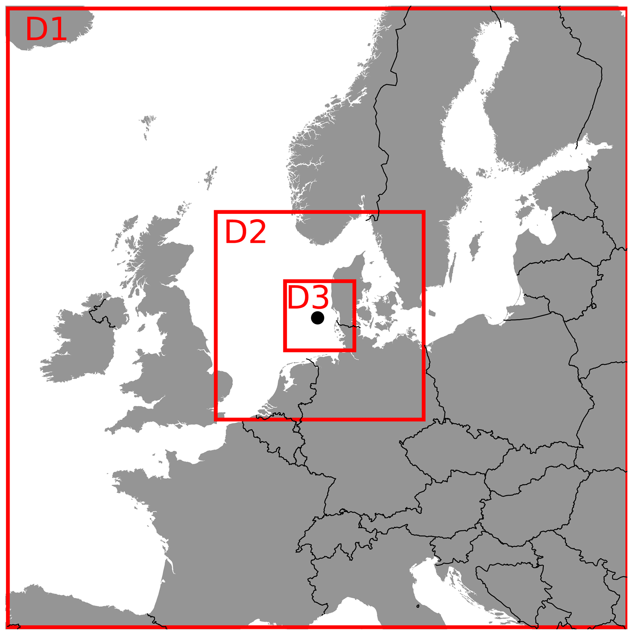
Figure 4 Mesoscale model domain distribution around the FINO3 site. The red boxes mark the extension of the computing domains. The coastline and border data originate from the GSHHS dataset (Wessel and Smith, 1996).

Boundary conditions for the model were prescribed by the ERA5 dataset for the atmospheric variables (Hersbach and Dick, 2016; Hersbach et al., 2020) and the OSTIA dataset for the sea surface variables (Donlon et al., 2012). An instantaneous output of the mesoscale model on 10 min intervals was chosen, being consistent with the 10 min means of the met masts.

Table 2 Relevant parameters of the setup for the mesoscale simulations applied in this study. The references for the different schemes and models are summarised in WRF Users Page (2020).

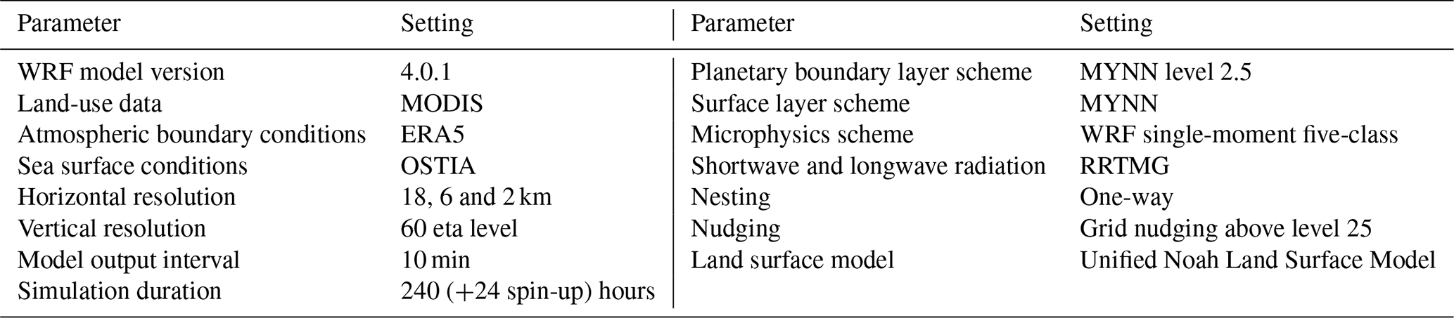
Table 2 shows a summary of the most important model set-up parameters and thus boundary conditions and model physics used in this study to drive the simulations. The output data on the WRF internal (Arakawa C, sigma terrain following) grid were converted to earth-relative quantities using the post-processing script developed and verified in the framework of the NEWA project⁴ (Dörenkämper et al., 2020). The data were interpolated to the exact measurement heights from the WRF levels, and virtual met masts were extracted at the grid point closest to the location of the met masts investigated in this study.

3 Applied procedures

The methods applied for our study are described in the following subsections and demonstrated on the basis of the FINO3 dataset.

3.1 Generation of artificial gaps

The first step of the analysis consists in generating artificial data gaps in the measured time series. This is demonstrated in Fig. 5 in the two upper plots. A data gap is defined by its length (in days or number of 10 min intervals) and its start. Figure 5 shows a gap of 30 d length starting on 30 September 2013, 00:00:00 UTC. For the results presented in Sect. 4 we have considered gap lengths between 6 and 90 d and start dates running through the 2-year measurement duration in equal increments. The four wind-energy-relevant statistical measures (mean wind speed and direction and Weibull shape and scale parameters) already presented in Sect. 2.1 are derived for the incomplete time series in the same way as for the original ones but ignoring the data in the gap. The deviations in these measures represent the impact of the gap on the wind statistics. Note that for this study we have only considered single gaps of varying lengths. Multiple gaps are briefly discussed in Sect. 5.

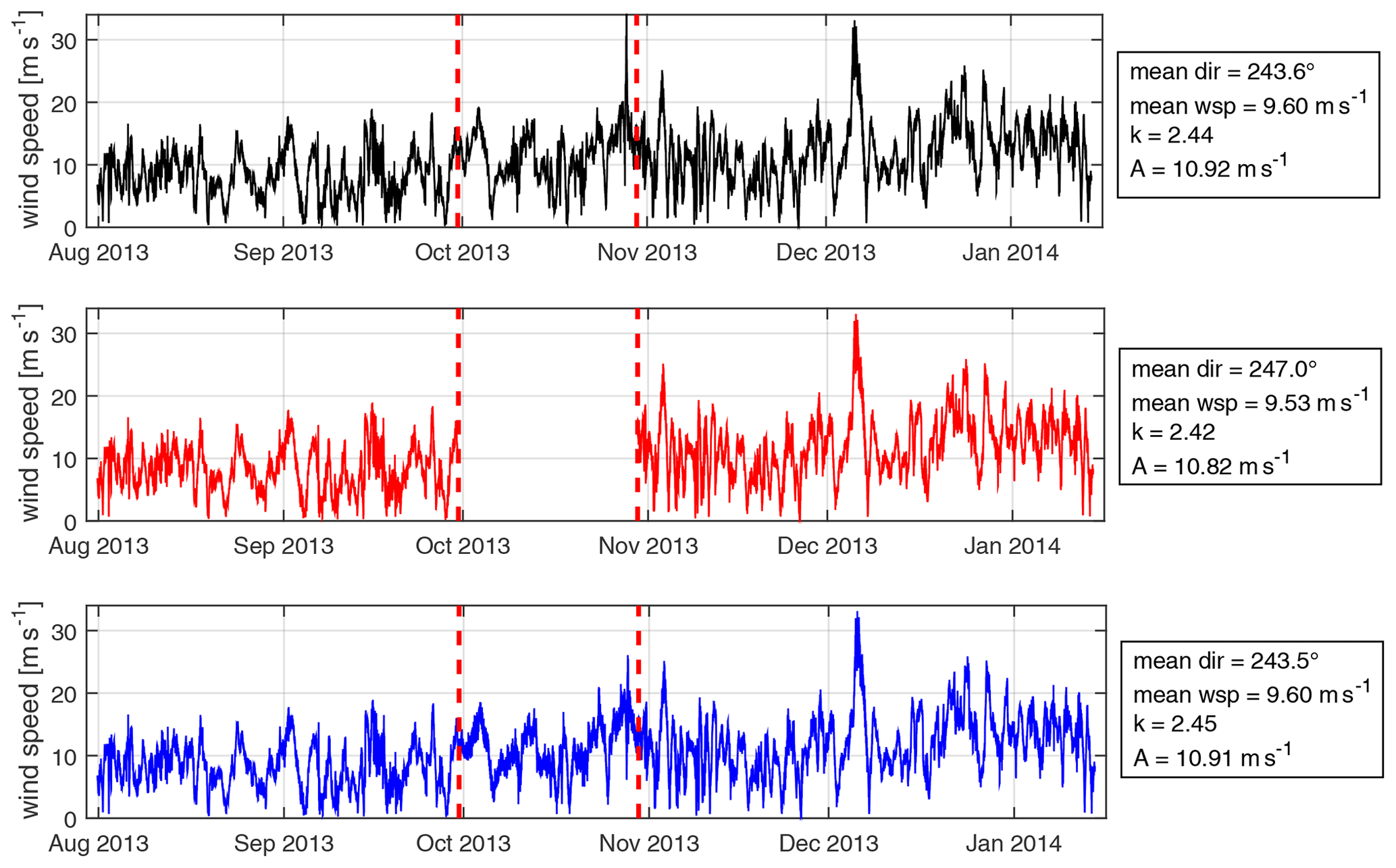
Figure 5 Generation and filling of artificial gaps – here demonstrated on the basis of the FINO3 wind speed time series and for a gap of 30 d length starting on 30 September 2013. Original time series (only an excerpt is shown) are in black, incomplete time series with a generated gap are in red and time series with a filled gap (see procedure described in 3.2) are in blue. Derived statistical measures (mean wind direction, mean wind speed, and k and A parameters of fitted Weibull wind distribution) are shown for the three time series on the right side.

3.2 Gap-filling procedure

The artificial gaps are filled based on a measure–correlate–predict (MCP) procedure and with the WRF data introduced in 2.2 as input. The measured time series consist of the wind speed and direction data including the generated gap, respectively. These data are correlated with the numerical (WRF) data for the same period. That is, for the period of the gap no data are considered for the correlation step. The correlation defines a correction that is implemented slightly differently for the wind speed and direction time series.

• For the wind speed data, we – first – bin the wind speeds every 0.5 m s⁻¹ based on the modelled data and calculate the average measured values in every bin. Second, we fit two linear functions for the wind speed ranges [0,5) and [5,20] m s⁻¹. The resulting coefficients of the linear fits are then applied to correct the respective modelled wind speed and in this way account for the systematic error between measured and modelled data.

• For the wind direction data, again first the mean deviation between measured and simulated wind direction per 10^∘ bin is derived and then used directly as offset for the correction.

Note that the choice of this approach is more or less arbitrary but motivated by current practice for similar studies and applications. No further procedural steps such as, for example, sector-wise corrections are considered.

In addition to the correction factor – resulting from either the correction function or the bin-wise mean offset – a noise factor is derived as the standard deviation of the data per bin and combined with a white-noise process in the prediction step. The noise factor ensures that the generated time series does not lose its physical consistency. For the prediction of the data in the gap period, numerical (WRF) data for this period are combined with the derived corrections. The resulting time series are inserted to the incomplete measurement time series.

Figure 5 (bottom plot) shows the outcome of the gap-filling procedure for the FINO3 time series used for demonstration.

As already mentioned above, the procedure consisting of generating artificial gaps in the measured time series and the filling with the outlined MCP approach is repeated for varying start dates of the gap that has a pre-defined length (in the example 30 d). This is demonstrated in Fig. 6, where the four derived statistical measures are shown for an unchanged gap length but systematically varying start date for the incomplete and filled time series (in red and blue). The wind statistics for the original time series are shown as a reference (as black lines).

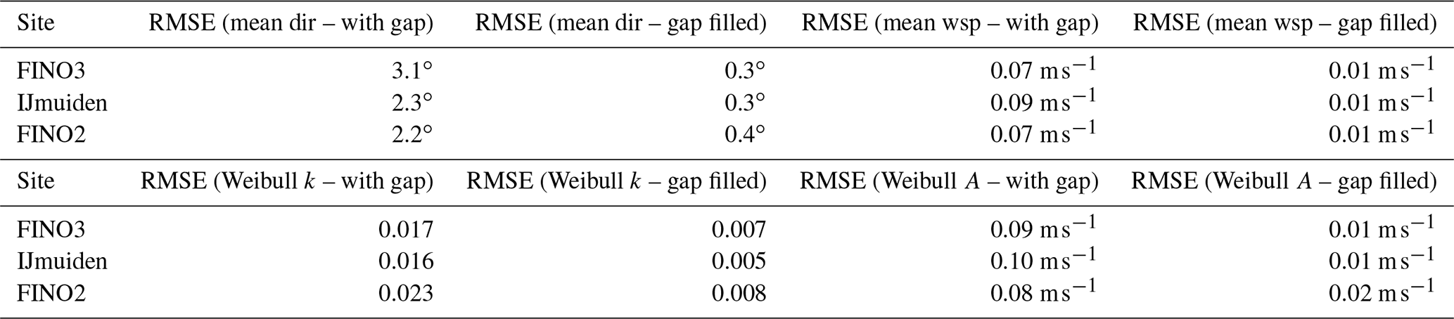
This example demonstrates that the impact of the generated gap varies quite drastically depending on when the gap starts, similar patterns are observed for all four considered statistical measures and the gap-filling procedure is able to significantly reduce the impact in almost all cases. However, the performance of the gap-filling procedure also depends on the start date of the gap. This can be explained by the fact that the correlation between measured and model data found on the basis of the existing data describes the correlation for the data of the gap to varying degrees. The correlation depends to a certain extent on seasonal effects, for example. To quantify the observed variations in the wind statistics, the corresponding root-mean-square error (RMSE) values are derived. For all four statistical measures, these reduce when the gaps are filled: for mean wind direction from 3.1 to 0.3^∘, for mean wind speed from 0.07 to 0.01 m s⁻¹, for the Weibull scale parameter A from 0.09 to 0.01 m s⁻¹ and for the Weibull shape parameter k from 0.017 to 0.007.

Figure 6 Variation in statistical measures – (a) mean wind direction and (b) mean wind speed and Weibull (c) shape and (d) scale parameters, k and A – depending on start date of artificial gap – here for a gap length of 30 d, for incomplete time series in red and for filled time series in blue. Wind statistics for the original time series are in black as reference.

Uncertainties or standard errors in the estimation of the parameters are not further considered here and in the following as they are small compared to the reduction of the gap impact, which is the focus of this study.

3.3 Long-term extrapolation

In a last step, the different time series are used as the basis for a long-term extrapolation of the wind time series and statistics. Therefore, the measured time series with or without data gaps are correlated with ERA5 reanalysis data that are available for a long-term period of 30 years in this case. The underlying MCP procedure is very similar to the one applied for the data gap filling in 3.2. But this time the correlation period corresponds to the total measurement period of 2 years in our case (for the incomplete time series shortened by the gap length), and the prediction horizon corresponds to the complete 30 years for which the reference data are available. The measured time series has to be resampled to 1 h data since the ERA5 data have no higher resolution. Otherwise, the same methods were used to derive and apply correction functions and offsets. As already pointed out above, we decided to use ERA5 data as long-term reference data (and not again WRF, which is also available for a period of 30 years in the New European Wind Atlas) because we believe this is a choice that still better corresponds to a typical case in a standard offshore wind resource assessment application, while the gap filling is still based on the mesoscale model data as before.

The overall workflow followed in the study is summarised in Fig. 7.

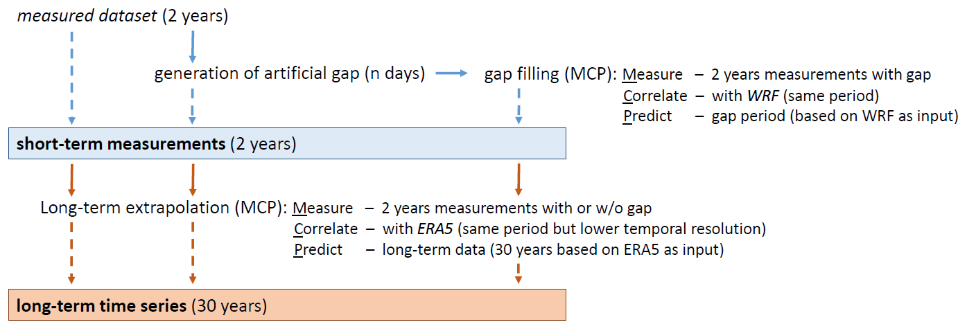
Figure 7 Workflow followed in our study including the MCP approaches for the gap-filling and long-term extrapolation procedures.

4 Results

In this section we present in detail the results of the study, expanding on the impact of gaps on the wind resource estimate with varying start dates (Sect. 4.1) as well as varying lengths (Sect. 4.2) and the impact of the gaps on the long-term wind resource estimate (Sect. 4.3). Results are compared for the three considered sites IJmuiden (Dutch North Sea), FINO2 (Baltic Sea) and FINO3 (German Bight).

4.1 Impact of gaps with varying start dates

Figure 8 shows how a 30 d gap impacts the four considered wind statistics (mean wind direction, mean wind speed, and the Weibull parameters k and A) depending on the start date of the gap for all three studied sites. The results for FINO3, already presented in Fig. 6, are shown in grey and the results for IJmuiden and FINO2 as dashed and dotted lines, respectively. Again, the applied gap filling (results in blue) reduces the deviations in the measures from the reference (in black) due to the existent gap (results in red) to a considerable degree. These reductions, quantified in terms of an RMSE for the respective dataset of results, are summarised in Table 3.

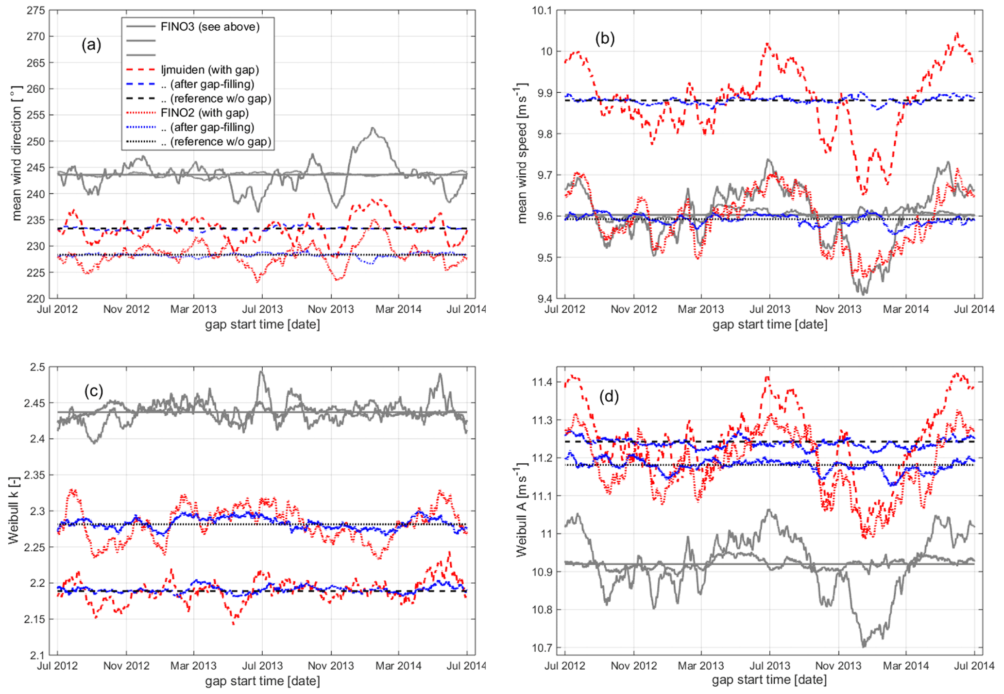
Figure 8 Variation in statistical measures – (a) mean wind direction and (b) mean wind speed and Weibull (c) shape and (d) scale parameters, A and k, respectively – depending on the start date of the artificial gap, here for a gap length of 30 d as in Fig. 6. Results for FINO3 (already presented above) as solid grey lines, for IJmuiden as dashed lines and for FINO2 as dotted lines (again for incomplete time series in red and for filled time series in blue and wind statistics for the original time series in black).

Table 3 RMSE derived for the four statistics considered in this study for time series with gaps and gap-filled time series of wind speed and direction for the three investigated sites.

For mean wind direction, mean wind speed and Weibull scale parameter A, the derived RMSE values, summarising the deviations in the wind statistics due to the gaps with varying start dates, reduce up to a factor of 10. For the Weibull shape parameter k this reduction is smaller (up to a factor of 3) which is explained by the nature of this parameter. Overall, the reductions are similar for all three considered sites. Also, the pattern of deviations in the wind statistics over the 2-year course are pretty similar, except those for the Weibull k parameter. Beyond that, Fig. 8 clearly shows how the wind statistics for the two sites FINO3 and FINO2, although having a very close mean wind speed for the considered 2-year period, differ with respect to their wind speed distributions and in particular the derived Weibull scale A and shape k parameters. The third site, IJmuiden, in comparison, is characterised by both the highest mean wind speed and Weibull A parameter and the lowest Weibull k parameter.

4.2 Impact of gaps of varying lengths

In the next step, we have repeated this analysis for different gap lengths between 6 and 90 d. Figure 9 shows the derived RMSE values for the four considered wind statistics (in four separate plots) and the three sites (as solid, dashed and dotted curves) plotted against the gap length, again for ignored and filled gaps (in red and blue).

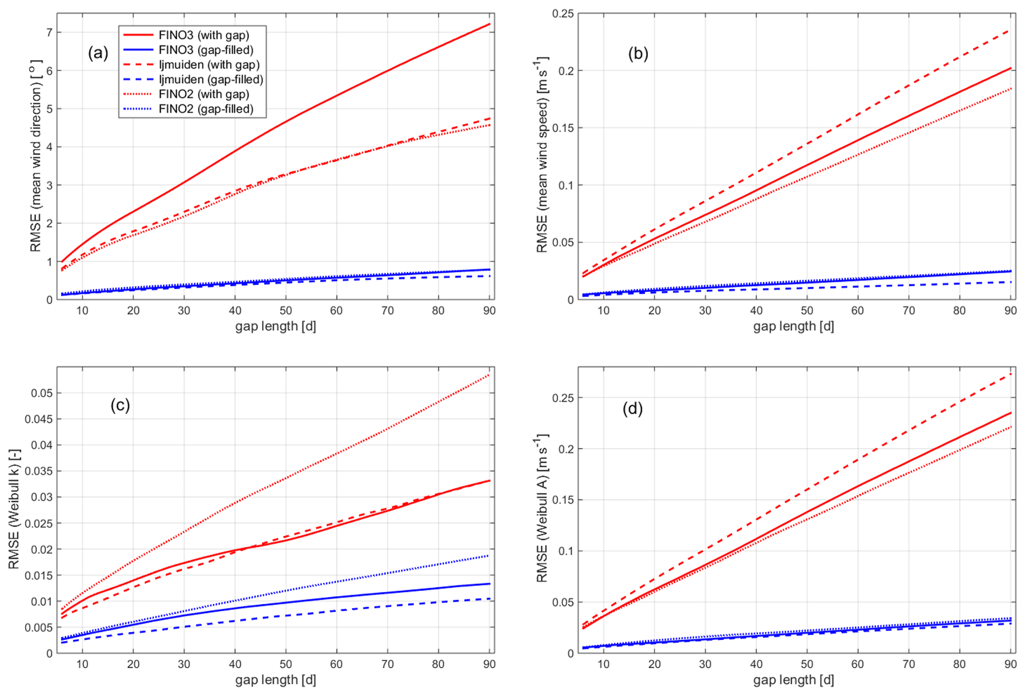
Figure 9 Dependency of impact of data gaps, quantified as RMSE of the four statistical measures – (a) mean wind direction and (b) mean wind speed and Weibull (c) shape and (d) scale parameters, A and k, respectively – derived for gaps with systematically varying start dates, on the length of the data gaps. Results for FINO3 as solid lines, for IJmuiden as dashed lines and for FINO2 as dotted lines (again for incomplete time series in red and for filled time series in blue).

In all considered cases, the impact of the gap (reflected by the derived RMSE) increases with gap length and is significantly reduced when applying the gap-filling procedure. For the mean wind speed, just like for the Weibull A parameter, the increase is more or less linear for the considered range up to 90 d, whereas it slightly flattens for the two other measures, mean wind direction and Weibull k.

Apart from these general agreements, the results for the three sites show some deviations. For instance, the impact of the data gaps on the mean wind speed are largest, when these are ignored, for the IJmuiden site but can be best compensated for. This is shown by the smallest RMSE values, compared to those for the two other sites, after gap filling. This observation may be explained by either the performance of the used numerical model for the respective site or a statistical effect that relates to the level of observed wind speeds. (Remember IJmuiden showed the highest measured mean wind speeds in the considered 2-year period.)

The impact of (ignored) gaps in the wind direction time series is highest for the FINO3 dataset. This can be understood by looking again at the wind direction distributions in Fig. 1: mean wind directions are more pronounced for the FINO2 and IJmuiden sites, whereas the distribution for FINO3 is characterised by a kind of site maximum for northwesterly directions. A data gap may in this case remove data that correspond to a substantial part of one of the local maxima, having a larger impact on the overall distribution as for the case where the distribution has only one superior maximum range. After gap filling, the RMSE values are still larger for the FINO3 dataset than for the IJmuiden data, but the deviations are now much smaller. RMSE values for FINO2 and FINO3 lie almost on top of each other.

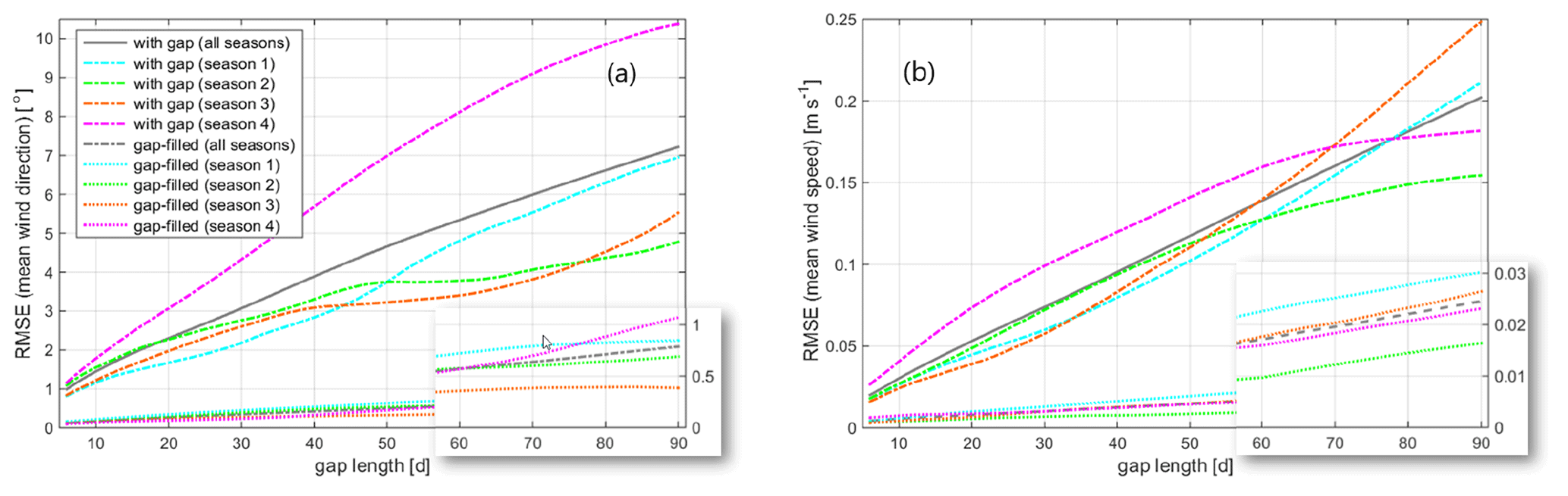
Figure 10 Dependency of impact of data gaps, quantified as RMSE, on the length of the data gaps and season (defined according to the gap start date) – as in Fig. 9 but here only for (a) mean wind direction and (b) mean wind speed. Results exemplarily for FINO3.

In a further step, we have studied how the impact of data gaps varies with the season in which the data gap occurs. For this, the ”season” is defined by the start date of a gap – a gap starting in the months of January to March is related to “season 1”, a gap starting between April and June to “season 2”, and so on. These seasons were selected with a shift of 1 month in comparison to the classical meteorological season definition of spring, summer, autumn and winter to consider the inertia of the heating–cooling of the sea surface that mainly drives the yearly cycle of the atmospheric stability which vice versa has an impact on the wind distribution.

Figure 10 shows the results for FINO3 and the statistics mean wind speed and mean wind direction only, but they are more or less also representative for the other cases. The plots clarify that the impact of ignored and filled gaps significantly depends on the assigned season whereby also the performance of the gap filling shows a certain dependency, but not always going in the same direction. Deviations are observed for not only the levels of derived RMSE values (i.e. how big is the impact) but also the shape of the curves (i.e. how does this change with gap length). This can be explained by the relation between gap length and the length of a season as defined above: a gap of a greater length is more likely to occur not just in the season it is assigned to. By this partly wrong assignment the seasonal effects are more mixed for the greater lengths.

4.3 Impact of gaps on long-term estimate

In a final step, we derive the impact of ignored and filled gaps in the measurement data on a long-term extrapolated mean wind speed. For this, we followed the procedure outlined in 3.3 and summarised in Fig. 7. Figure 11 shows how the mean wind speed that is derived based on 30 years of ERA5 data and corrected according to the 2-year-long measurements at the three considered sites varies with the start date of a 30 d data gap that is cut into the measurement time series. Again the data gaps are either ignored (results in red) or filled by applying the introduced gap-filling procedure (results in blue).

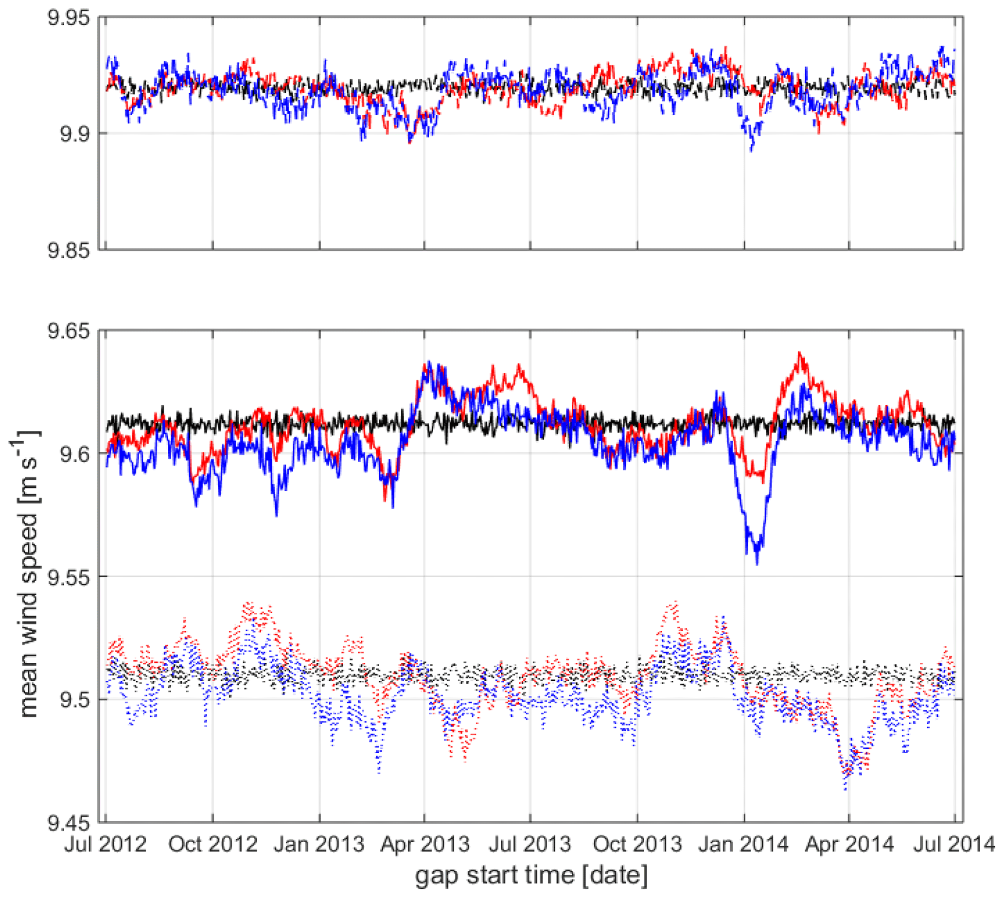
Figure 11 Variation in long-term corrected mean wind speed depending on start date of the artificial 30 d gap in short-term measurements. Results for FINO3 as solid lines, for IJmuiden as dashed lines and for FINO2 as dotted lines (again for incomplete short-term measurement time series in red and for filled time series in blue and for measurements without gap in black as reference).

The following conclusions can be drawn from Fig.  11.

• The long-term corrected mean wind speed is significantly different from the mean values of the 2 years of measurements for the three considered sites. (Mean wind speed values of the used 30-year-long ERA5 time series are 9.43, 9.91 and 9.26 m s⁻¹ for FINO3, IJmuiden and FINO2, respectively.)

• The impact of data gaps in the short-term measurements is visible in the long-term estimates but is rather small with an RMSE (for ignored gaps, red curves) of 0.011 m s⁻¹ (FINO3), 0.007 m s⁻¹ (IJmuiden) and 0.014 m s⁻¹ (FINO2).

• This impact of the data gaps in the short-term measurement on the long-term estimates is not really mitigated through the application of the gap-filling procedure; corresponding RMSE values (for filled gaps, blue curves) are in the same range or even slightly larger with 0.015 m s⁻¹ (FINO3), 0.008 m s⁻¹ (IJmuiden) and 0.014 m s⁻¹ (FINO2).

• Also, the reference values (black curves) show some variability, which is due to the noise process as part of the MCP procedure applied for the long-term extrapolation. The RMSE values reflecting these variations are equal for all three sites with 0.003 m s⁻¹ where the mean value is considered as reference.

5 Discussion

Our study proposes a methodology that allows us to quantify the impact of data gaps in (measured) time series on wind statistics. With the three studied sites, we have considered three possible reference datasets, which could be referred to for further sites where only incomplete time series are available but no suitable reference. The reference quantification can then be used to deduce an uncertainty associated with the inherent gaps, which could be related to the RMSE value derived for the variations in the wind statistics for different gap start dates for a fixed gap length. Alternatively, for a more conservative approach, the maximum deviations in the wind statistics observed in the reference study could be considered or, in case more details are available, the identified variations for a specific season could be considered.

For our study, we have analysed the four statistical measures mean wind direction, mean wind speed, and the two Weibull parameters k and A which are very common for siting applications – but in principle this selection has been arbitrary and can be further extended. Another common measure frequently considered in the wind energy context is the wind power density (WPD), as defined in Chang (2011), which integrates the two Weibull parameters (A and k) according to

$$\begin{array}{}\text{(1)}& \text{WPD}={\displaystyle \frac{\mathrm{1}}{\mathrm{2}}}\mathit{\rho }{A}^{\mathrm{3}}\mathrm{\Gamma }\left(\mathrm{1}+{\displaystyle \frac{\mathrm{3}}{k}}\right),\end{array}$$

with the air density ρ and the gamma function $\mathrm{\Gamma }\left(x\right)={\int }_{\mathrm{0}}^{\mathrm{\infty }}{e}^{-t}\cdot t^{x-\mathrm{1}}\mathrm{d}t$.

In Fig. 12, we show the results for WPD as for the other measures in Fig. 6. Again, it is clear to see how the gap-filling procedure reduces the impact of the data gaps. The reduction is smaller than for the Weibull parameter A but larger than for k with an RMSE value decreasing from 21.2 to 5.0 Wm⁻².

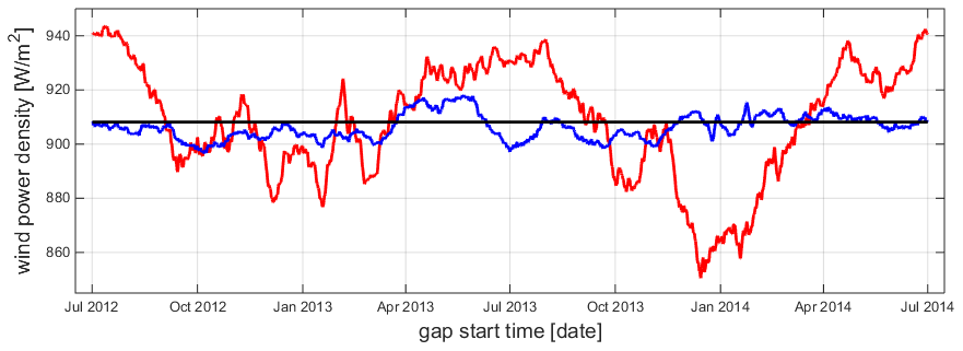
Figure 12 Variation in wind power density (WPD), as an alternative statistical measure to those shown already in Fig. 6 for the FINO3 site, depending on start date of artificial gap – here for a gap length of 30 d, for incomplete time series in red and for filled time series in blue. Wind statistics for original time series are in black as reference.

In the presented investigations, we have only considered isolated single gaps in a measured time series. But the approach followed can be extended, in a straightforward way, to more complex scenarios including multiple gaps that may be more realistic or may correspond to a specific case of interest. We would then recommend the following procedure: the present scenario would first be generalised to an extent so that the available reference study case is sufficiently informative. If we want to evaluate the impact of a 20 d gap in February of a certain year, for instance, it may not be sufficient to study the impact of such a gap in the reference data from another period only for the month of February. Instead the scenario may be broadened to a 20 d gap in the winter season. For making this decision, some background knowledge of the general wind climate at the studied sites is required, which can be gained from (numerical) long-term datasets. A similar approach is recommended for the consideration of multiple gaps, for which not only the lengths of the individual gaps need to be taken into account but also their distance in time and possible correlation effects.

With carrying out the study for three different offshore sites and showing the systematic similarities and some deviations between the results, we provided a basis for the selection of suitable reference sites and datasets. Again, some knowledge of the general wind climate at a site is required to evaluate whether a certain study site is suitable or not for the estimation of an uncertainty that is then used for the evaluation of the measurements from another site. In general, however, we believe that this transfer of observations is possible and suggest using the available sites and datasets for this purpose. An extension of our study to further sites, moreover, may help to better understand how the impact of data gaps on wind statistics may vary from site to site and to take such findings into account for an even more refined estimation of the associated uncertainties.

When looking at the mitigation of the impact of data gaps in the measured time series – explicitly, with the applied gap-filling procedure and the use of an MCP procedure in connection with wind data from a numerical model – we have only applied one specific method but not further studied how the results may change with the application of other approaches. In this context, it was important for us to have a procedure that is straightforward and easy to apply for all three sites in exactly the same way. But we definitely also believe that a refinement – e.g. by using more complex approaches and possibly also some fine-tuning for the individual sites – may show an optimised performance and with this less remaining impact of the data gaps on the wind statistics after gap filling. We believe that a specific gap-filling approach should be an integral part of the wind resource assessment process that is applied by a specific consultant for a specific site as it improves the wind statistics of the measured period and can potentially also reduce the uncertainty of the long-term assessment.

It should also be pointed out that it is possibly not the optimal approach to apply the same type of MCP procedure for both the gap-filling and the long-term extrapolation steps. Depending on whether the simulation of time series (i.e. for a point prediction or filling gaps) or the simulation of a wind distribution or wind statistics is of interest, so-called type I or type II MCP methods may be the better choice (Hanslian, 2017). In short, type I MCP methods are designed to simulate time series whereas type II methods generate wind distributions. Whichever method is selected for the specific MCP task, this method should also be applied in the reference study to quantify the gap impact and estimate the associated uncertainty that is of high relevance for the (here: wind energy) application in any case.

The fact that we have not optimised the MCP methods for our applications may also be the reason for the initially counter-intuitive observation that the gap-filling procedure, applied to the short-term measurements, has no positive effect on the long-term extrapolated results (see 4.3). Another reason is the relatively short gap of only 1 month which is still within the availability of >90 % accepted by MEASNET. Furthermore, if we compare the deviations in Figs. 8 and 11, we see that the fluctuations in the long-term average are on the order of magnitude of the gap-corrected values and not on that of the uncorrected values. This means that the long-term correction already averages out the effects of the data gaps to some extent, so that the gap filling is no longer significant.

Finally, it must also be kept in mind that the quantified uncertainty is – when looking at the complete wind resource assessment process – not the only uncertainty that is associated with the long-term extrapolation. Another substantial uncertainty component arises from the fact that the considered short-term period for which on-site measurements are available has only a limited representativeness for the long term. Some of this is compensated for by the long-term extrapolation based on a “long” dataset itself, but it needs to be considered that a derived correction function always has some dependency on the available correlation period. This dependency and related variations in the results of the estimated wind statistics constitute another part of the uncertainty associated with the long-term extrapolation, not yet taken into account, in a wind resource assessment.

6 Conclusions

As any field experiment, wind measurements that are typically carried out for site assessment studies are subject to data gaps due to failures of measurement devices or data loggers. In the harsh offshore wind climate, wind and wave conditions can lead to considerable time windows of inaccessibility of the measurement platform no matter whether floating, e.g. buoy, or mast measurement. In our study we investigated the impact of these data gaps on typical statistical measures for wind energy siting applications such as mean wind speed and direction and the Weibull shape and scale parameters. The study was performed for three offshore sites with meteorological mast measurements available between July 2012 and June 2014 in the southern North Sea (FINO3 and IJmuiden) and the southern Baltic Sea (FINO2). We proposed a gap-filling procedure that uses data from mesoscale meteorological modelling and studied the benefit of the gap filling in terms of the RMSE of the siting statistics. The study reports the following key results.

• A gap of 30 d in the dataset leads to an RMSE on the mean wind speed of up to about 0.1 m s⁻¹ in the mean wind speed and the Weibull scale parameter A, an RMSE of about 0.02 on Weibull shape k and 3^∘ in the mean wind direction.

• The gap filling with mesoscale data can considerably reduce this impact up to a factor of 3 on the Weibull shape and a factor of 10 on the three other investigated siting parameters mean wind speed, direction and Weibull scale.

• The impact of the data gaps is monotonically and almost linearly increasing with the length of the data gap when considering the full year wind climate and so is the reduction of the impact of the gap filling. However, when looking at different seasons, the skill of the gap filling differs.

• The key conclusions are similar for the three investigated sites, although the impact of gaps differs with the highest impact on the data from the FINO3 mast that is the only mast with a prominent impact of northwesterly winds and also the mast that is located furthest offshore.

• The impact of the gaps on the long-term estimate, expressed here in terms of a 30-year wind climatology, is very small (around 0.01 m s⁻¹ at all three sites) and cannot be substantially further reduced by the gap filling of the reference measurement dataset.

Our investigation focused on three European offshore sites in the North Sea and Baltic Sea and could in future studies be evaluated for other offshore exploration areas with more different wind distributions in speed and direction. We intentionally focussed on three commonly used key wind energy siting statistics. With the tendency of a grid-load-based renumeration of wind power, an investigation of the impact of data gaps on daily cycles might be interesting for future investigations.