Active flap control with the trailing edge flap hinge moment as a sensor: using it to estimate local blade inflow conditions and to reduce extreme blade loads and deflections

Active trailing edge flaps are a promising technology that can potentially enable further increases in wind turbine sizes without the disproportionate increase in loads, thus reducing the cost of wind energy even further. Extreme loads and critical deflections of the blade are design-driving issues that can effectively be reduced by flaps. In this paper, we consider the flap hinge moment as a local input sensor for a simple flap controller that reduces extreme loads and critical deflections of the DTU 10 MW Reference Wind Turbine blade. We present a model to calculate the unsteady flap hinge moment that can be used in aeroelastic simulations in the time domain. This model is used to develop an observer that estimates the local angle of attack and relative wind velocity of a blade section based on local sensor information including the flap hinge moment of the blade section. For steady wind conditions that include yawed inflow and wind shear, the observer is able to estimate the local inflow conditions with errors in the mean angle of attack below 0.2^∘ and mean relative wind speed errors below 0.4 %. For fully turbulent wind conditions, the observer is able to estimate the low-frequency content of the local angle of attack and relative velocity even when it is lacking information on the incoming turbulent wind.

We include this observer as part of a simple flap controller to reduce extreme loads and critical deflections of the blade. The flap controller's performance is tested in load simulations of the reference turbine with active flaps according to the IEC 61400-1 power production with extreme turbulence group. We used the lifting line free vortex wake method to calculate the aerodynamic loads. Results show a reduction of the maximum out-of-plane and resulting blade root bending moments of 8 % and 7.6 %, respectively, when compared to a baseline case without flaps. The critical blade tip deflection is reduced by 7.1 %. Furthermore, a sector load analysis considering extreme loading in all load directions shows a reduction of the extreme resulting bending moment in an angular region covering 30^∘ around the positive out-of-plane blade root bending moment. Further analysis reveals that a fast reaction time of the flap system proves to be critical for its performance. This is achieved with the use of local sensors as input for the flap controller. A larger reduction potential of the system is identified but not reached mainly because of a combination of challenging controller objectives and the simple controller architecture.

1 Introduction

Wind turbines have increased dramatically in size over the past years in an effort to reduce the cost of wind energy and make it a competitive source of energy. The increased installation numbers of new wind turbines in Germany over the years is an example of the success that this strategy has had (Burger, 2018). Increasing the turbine size also has its drawbacks. A larger rotor will see increased loads that cannot be compensated for by a geometric upscaling of the components alone (Jamieson, 2018, 97–123). In order to withstand these loads, the structure of turbine components such as the blade has to be stiffer, which requires more material or stronger (and more expensive) material. This results in an increase in cost of energy. Advanced turbine controllers counteract the increased loads of larger turbines, thereby limiting the need for additional material and decreasing the cost of energy. The most widely used actuator for load reduction is the pitch actuator. Its main advantage is its availability because it is already being used in the power regulation strategy. Yet it has several drawbacks regarding load control. As wind turbines become larger, the frequency bandwidth of their pitch actuators is reduced mainly due to the increased inertia of the blade. This reduces the ability of current advanced load-reduction controllers – based on full span pitch control – to react to sudden local wind gusts and to fast-changing turbulent inflow, thereby limiting their effectiveness. Loads arising from non-uniform wind fields (e.g., wind shear and turbulence) have a greater effect in larger turbine rotors (Madsen et al., 2020). Such effects are better countered with spatially distributed actuation devices than with an actuator for the whole blade, as is the case for the pitch system.

A promising alternative to conventional full span pitch control is the concept of the smart rotor with distributed active flow control (AFC) devices. Barlas and van Kuik (2010) give an overview of the different control concepts, actuators and sensors that are relevant for active load alleviation in smart rotors. The authors conclude that trailing edge (TE) flaps and microtabs are the most promising actuation concepts. This comes from their ability to effectively change the local lift, their high actuation bandwidth and the simplicity considering their implementation.

1.1 Sensors for active flap control

In addition to AFC actuators, the choice of AFC sensors is another critical aspect for the load alleviation strategies of smart rotors. Cooperman and Martinez (2015) give a review of the possible sensors that can be used in smart rotor control. Many of these sensors have been used in TE flap control studies over the past years. We can broadly categorize them into three groups: strain sensors, inertial sensors and inflow sensors.

• Strain sensors measure the local strains on a component. These can be conventional strain gauges or optical strain sensors. Strain sensors have been widely used in TE flap control strategies. In particular, strain sensors measuring the flapwise blade root bending moment (BRBM) have received much attention. A common strategy that uses these sensors is called individual flap control (IFC). It is based on the individual pitch control (IPC) strategy (Bossanyi, 2003) and is often used in combination with the latter (Plumley et al., 2014b; Lackner and van Kuik, 2010; Plumley et al., 2014a; Jost et al., 2015; Bernhammer et al., 2016; Zhang et al., 2016). Other studies have used the flapwise BRBM sensor in PID-type controllers (Barlas et al., 2016b; Bartholomay et al., 2018), model-based controllers (Henriksen et al., 2013; Bergami and Poulsen, 2015; Chen et al., 2016; Ng et al., 2016) and adaptive controllers (Navalkar et al., 2014).

• Inertial sensors are able to measure the motion of a component resulting from a force. The most common inertial sensors are accelerometers. They offer the advantage of sensing the effect of the loads before any deflections and strains have occurred. If used for TE flap control, these sensors give the controller potentially more time to react to sudden disturbances. Integrating the acceleration values gives information about the velocity and displacement of the component.

  Zhang et al. (2016) compare the performance of IFC strategies based on acceleration and deflection signals to the more traditional IFC based on the flapwise BRBM. In Berg et al. (2009) and Engels et al. (2010), the authors implement TE flap controllers that use the blade tip deflection/deflection rate with a PD or PID feedback loop to control the flaps. This strategy is also used in Wilson et al. (2009), where the combination of IPC and the aforementioned feedback flap control is explored. In the INNWIND report (Jost et al., 2015), a similar control strategy that uses the low-passed blade tip acceleration as input for a PI feedback loop that sets the flap angle is implemented. A model predictive controller (MPC) for TE flaps based on local blade displacement is used in Barlas et al. (2012).

• Inflow sensors are able to measure the local aerodynamic conditions of a blade section. They are attractive because they are able to measure the source of the aerodynamic loads on a specific blade section before they affect the section. This gives the TE flaps more time to react to aerodynamic disturbances and hence to reduce the loading. Local inflow sensors on the blade include pitot tubes and surface pressure sensors. A drawback of pitot tubes is that they might vibrate during operation or be affected by rain, ice, dirt or insects. Both factors diminish the accuracy of the measurements or in extreme cases disrupt them. Surface pressure sensors can be expensive and fragile and may be clogged during operation (Cooperman and Martinez, 2015). Other types of inflow sensor are remote inflow sensors and nacelle-mounted sensors. An example of the former are lidar sensors while spinner-mounted anemometers are an example of the latter.

  Bartholomay et al. (2021) analyze the load reduction capabilities of feed-forward flap controllers on a 2D airfoil in a wind tunnel. The controllers estimate the lift acting on the airfoil by means of either a pitot tube or three surface pressure ports. Barlas et al. (2018) test an active flap system on a 2 m blade part mounted on a rotating test rig. They demonstrate the load alleviation potential of the system using an open-loop controller based on local inflow measurements. Andersen (2010) studies several control strategies based on local inflow measurements and their combination with strain gauges placed along the blade span. Barlas et al. (2012) also considered an extension of the MPC strategy that measured the local inflow of the blade section. Jones et al. (2018) use a blade-mounted pitot tube in addition to the blade root strain gauges as an addition to an IPC strategy. The use of the inflow sensor in a cascaded configuration helps improve the performance of the controller by bypassing the limitations of the slow blade dynamics on the controller input.

  Manolas et al. (2018) combine an IPC strategy with a feed-forward TE flap controller based on the inflow measurements of a spinner-mounted anemometer. Ungurán et al. (2018) use a combination of a model-based feedback individual pitch and flap controller and a model-inverse-based feed-forward controller that uses the blade effective wind speed measured with a blade-mounted lidar system.

1.2 Active flap fatigue control and blade design driving loads

Strain sensors measuring the flapwise BRBM have been a popular and effective choice because the main focus of TE flap control has been fatigue load reduction of the out-of-plane loads. The frequency content of these fatigue loads is fairly low (Bergami and Gaunaa, 2014). Therefore, these sensors can be effectively used even if they measure the effect of the aerodynamic loads with a certain delay (caused by the blade inertia).

Out-of-plane fatigue loads are design driving for several turbine components. Yet if we focus on the wind turbine blade, flapwise fatigue loads are not necessarily the best objective to use TE flaps or other local AFC devices for.

• Flapwise BRBM fatigue loads have a fairly low-frequency content. Most of the damage concentrates around the 1P frequency (Bergami and Gaunaa, 2014) and can be addressed by the pitch controller using strategies such as IPC.

• Using TE flaps to mitigate 1P and 2P flapwise BRBM means that the high bandwidth capabilities of these actuators are not used effectively.

• Using AFC for fatigue load reduction requires a high number of duty cycles of the actuator. This is a limiting factor in the choice of the actuator. It is also not in line with the current philosophy of wind turbine designs since wind turbines are designed to be low maintenance machines. Having a high number of duty cycles might result in high maintenance requirements for the AFC actuator.

Blade optimization studies that include fatigue-oriented TE flap control as part of their optimization features did not show significant additional blade mass reduction compared to an optimized blade design without flaps. Barlas et al. (2016a) optimize the DTU 10 MW Reference Wind Turbine-blade (Bak et al., 2013) using a multidisciplinary design, analysis and optimization tool. They find that the results of the blade optimization are comparable if the blade is optimized with a fatigue-focused flap controller or if the blade is optimized without flaps altogether. Chen et al. (2017) use an optimization algorithm to optimize the blade of the NREL 5 MW Reference Wind Turbine (Jonkman et al., 2009) so that the levelized cost of energy is minimized. The algorithm also optimizes a model-based controller used for pitch and TE flap control (Chen et al., 2016). They conclude that

[t]he blade optimization problems addressed in this work are primarily driven by flapwise stiffness, with blade deflection, rotor thrust and flapwise ultimate stresses in the spar forming the design drivers (Chen et al., 2017, p. 764).

Chaviaropoulos et al. (2014) point out that important load components for preliminary innovative concepts of multi-megawatt-scaled turbines include the ultimate loads of the resulting BRBM, ultimate and fatigue loads of the blade root torsional moment, fatigue loads of the edgewise BRBM, and the blade tip-to-tower clearance.

From these findings one can conclude that for modern large rotor blades, the extreme value of the resulting BRBM and the blade tip-to-tower clearance will be decisive. In the edgewise direction, the design-driving loads will be dictated by the fatigue loads arising from the blade's mass. In this direction, the blade root has to endure a load fluctuation with an amplitude equaling the blade's static moment once per revolution (1P).

1.3 Active flap control for reducing extreme blade loads and deflections

Should the objective of an AFC strategy shift to reducing flapwise extreme loads and critical deflections, it would also have a positive effect on the design-driving edgewise fatigue loads of the blade. When an effective controller reduces extreme loads and deflections, the spar cap of the blade can be optimized and hence the mass of the blade reduced. This in turn reduces the edgewise fatigue loads near the blade root. These loads are mainly caused by gravitational forces. In additional optimization loops, the blade mass could be further reduced, potentially creating a virtuous cycle.

If a TE flap control strategy is used to alleviate loads with high frequency content (such as design-driving extreme loads), the choice of a sensor for controller input becomes much more relevant. Using the flapwise BRBM as an input sensor for the TE flap controller has its advantages in the implementation and maintenance of the sensor but can have negative effects on the performance of the controller. Because sensor and actuator are far apart, aerodynamic loads and deflections at the blade tip are sensed at the root with a considerable time lag. This time lag carries through to the actuation response of the controller, limiting its effectiveness (Andersen et al., 2010; Fisher and Madsen, 2016; Jones et al., 2018). Inflow sensors would be an attractive sensor choice were it not for the practical drawbacks of cost (e.g., lidar) or susceptibility to the elements (e.g., pitot tubes and pressure sensors) in their implementation (Cooperman and Martinez, 2015).

A possible sensor that has not received much attention from the community is the TE flap hinge moment (Behrens and Zhu, 2011). It has the advantage of providing local loading information of a blade section without the need of additional inflow sensors on the blade. The flap actuator is assumed to be enclosed inside the blade section. This protects the hinge moment sensor (located in the actuator) from the elements, making it a very robust sensor. The loading information from the flap hinge can be used in combination with the high actuation bandwidth of the flaps to effectively reduce extreme loads and critical deflections of the blade. This idea is attractive because it uses the robust and already available hinge moment sensor in the flap actuator system as an input for the controller, thus addressing the aforementioned drawbacks of cost and susceptibility. It is also advantageous if the TE flap system is to be designed in a modular layout.

The goal of the present study is to explore and quantify the potential of TE flaps to mitigate design-driving extreme loads and deflections. We are also interested in exploring the possibility of using a local and robust sensor as an input choice for a controller strategy. This paper presents a novel method that allows the use of the TE flap hinge moment as an input sensor. It is a model-based observer that estimates the effective angle of attack of the blade section given the hinge moment, the accelerations and the relative wind velocity of the section (the last quantity is also estimated with our method). In addition, we use this observer as part of a simple extreme load controller for flaps and analyze its performance in a power production scenario with extreme turbulent wind. Section 2 summarizes our turbine and flap models as well as the aeroelastic simulation tools used in this study. In Sect. 3, we present the model used to calculate the unsteady flap hinge moment in aeroelastic simulations and our novel observer that estimates the local aerodynamic information based on this and other sensors. Section 4 presents the results of the observer under steady and turbulent wind conditions. In Sect. 5, we present a simple extreme load controller that uses this observer. We analyze the controller's performance in reducing extreme loads under challenging extreme turbulent wind conditions. The conclusions are drawn in Sect. 6.

2 Methods

The DTU 10 MW RWT was chosen as the turbine model. It is representative of the new generation of wind turbines and has been used in several research studies. The complete description of the turbine can be found in Bak et al. (2013).

2.1 Blade with trailing edge flaps

The blade of the DTU 10 MW RWT was modified to accommodate TE flaps. The flaps are modeled via dynamic polar sets that describe the airfoil with discrete flap angles. For this study we chose a flap that covers 10 % of the chord and has maximum deflection angles of $\mathit{\delta }=\pm \mathrm{15}$^∘. Figure 1a shows the polar data of the FFA-W3-241 airfoil – used in the outer part of the blade – with the modeled flap at maximum and minimum deflection. In total 15 polar sets were generated for different discrete flap positions using a Reynolds number of 1.5×10⁷. The polars were obtained using the airfoil simulator XFLR5 integrated into QBlade (Marten et al., 2010). In the simulation, the polar data between the discrete states are linearly interpolated.

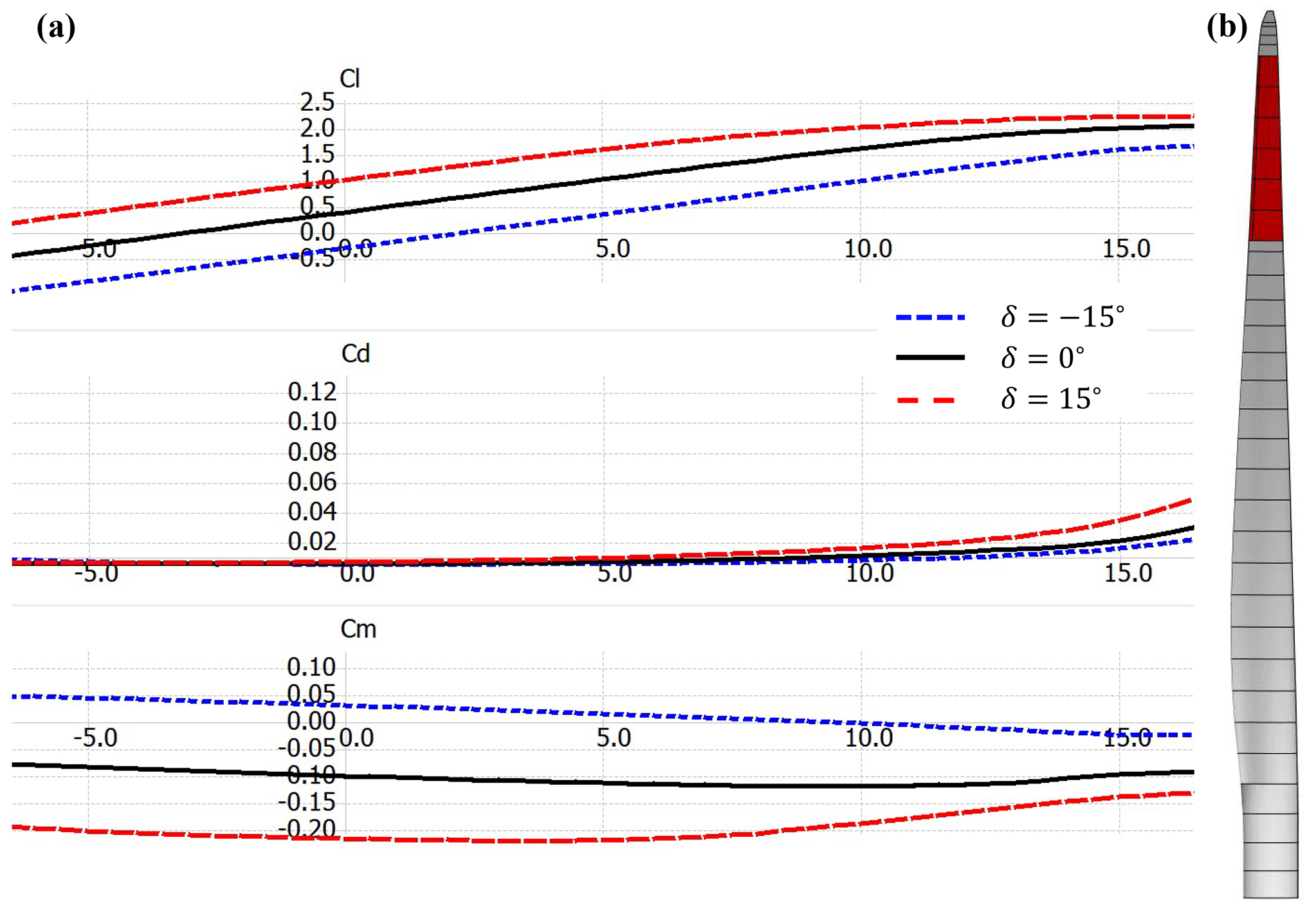
Figure 1 Trailing edge flaps on the DTU 10 MW RWT blade. (a) FFA-W3-241 airfoil polars with different flap deflection angles. (b) Position of the six flaps on the blade.

In total six flaps are integrated into the blade, as can be seen in Fig. 1b. Each section measures 3 m in the spanwise direction and is assumed to have one hinge moment sensor and one accelerometer located at the center of the section. The six sections are located between 64 and 82 m of the blade span, which corresponds to a relative location between 74.1 % and 95 % of the blade length. The flap actuators are modeled as a second-order low-pass filter. In the Laplace domain, the filter takes the form

$$\begin{array}{}\text{(1)}& {\mathit{\delta }}_{\mathrm{LP}}\left(s\right)={\displaystyle \frac{{\mathit{\omega }}^{\mathrm{2}}}{s^{\mathrm{2}}+\mathrm{2}\mathit{\xi }\mathit{\omega }\cdot s+{\mathit{\omega }}^{\mathrm{2}}}}\cdot \mathit{\delta }\left(s\right),\end{array}$$

where ω is the filter frequency and ξ the damping factor. For the flap actuators, we chose a frequency of 5 Hz and a damping factor of 1. The maximum and minimum flap rates are limited to ±100 ^∘ s⁻¹.

2.2 Aeroelastic simulation tools

We did the development, testing and simulation of the methods presented in this study using two aeroelastic simulation tools: the first is NREL's FAST v8.15 and the second is TU Berlin's QBlade.

2.2.1 FAST

FAST uses AeroDyn (Moriarty and Hansen, 2005) as its aerodynamic model. It is based on the blade element momentum (BEM) theory and uses several correction models to account for the unsteady aerodynamic phenomena typically present in aeroelastic simulations with turbulent conditions. These are the tip- and root-loss model, the turbulent wake state model, the oblique inflow model, the dynamic stall model, and the tower shadow model.

The used structural model in FAST is ElastoDyn. It has a combined multi-body and modal dynamics representation that is able to model the wind turbine with flexible blades and tower (Jonkman, 2003).

2.2.2 QBlade

QBlade uses the lifting line free vortex wake (LLFVW) method as its aerodynamic model (Marten et al., 2015). In this method, the blade aerodynamic forces are evaluated on a blade element basis using polar data. The near and far wake are modeled with vortex line elements. These are shed at the blade's trailing edge during every time step and then undergo free convection behind the rotor. Vortex methods can model the wake with far fewer assumptions and engineering corrections compared to BEM methods. Especially when the wind turbine is subjected to unsteady inflow or varying blade loads, the LLFVW method increases the accuracy compared to BEM methods (Perez-Becker et al., 2020). To model the dynamic stall of the blade elements, QBlade uses the ATEFlap unsteady aerodynamic model (Bergami and Gaunaa, 2012), modified so that it excludes contribution of the wake in the attached flow region (Wendler et al., 2016).

QBlade is able to model AFC devices such as TE flaps using two dynamic polar sets. They are defined for the inner and outer spanwise locations of the AFC device. It is thereby possible to model AFC elements that span over two different airfoils. The ATEFlap model is also capable of modeling unsteady aerodynamic effects of flap deflections at high reduced frequencies. This allows QBlade to accurately model the aerodynamics of TE flap actuators with high bandwidths. This is required if a flap control strategy aims at reducing extreme loads and deflections.

QBlade has a structural solver based on the open-source multi-physics library CHRONO (Tasora et al., 2016). It uses a multi-body representation which includes Euler–Bernoulli beam elements in a co-rotational formulation. It allows QBlade to accurately simulate the blade deflections and include the blade torsion, which has a significant influence on the blade loads.

A more detailed comparison between QBlade and (Open)FAST can be found in Perez-Becker et al. (2020).

Figure 2 Sketch showing the angles and coordinate systems of a 2D airfoil section. The blade section is depicted at a rotor azimuth angle φ=90^∘. The colors of the deflected flaps correspond to the polar data of Fig. 1.

2.3 Controller

For this study, we used the TUB Controller (Perez-Becker et al., 2021). It is based on the DTU Wind Energy Controller (Hansen et al., 2013), which features a baseline pitch and torque control. It has been extended with a supervisory control based on the report by Iribas et al. (2015). The supervisory control allows the controller to run a full load analysis. The controller baseline pitch and torque control parameters were taken from the report by Borg et al. (2015). The controller has been extended so that it can control AFC devices such as TE flaps.

3 Estimation of the aerodynamic information

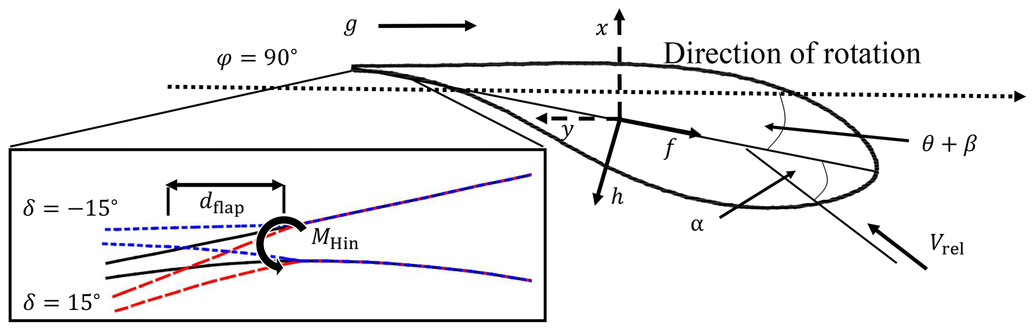
In this section we present the flap hinge moment model used in this study and the observer based on this model. The latter is able to estimate the effective angle of attack and relative velocity of a flapped blade section by means of local and global sensors, the former being an accelerometer, a flap position sensor and the flap hinge moment sensor. These sensors and the hinge are assumed to be positioned at the span-wise center of the blade section with active flap. The global sensors are the rotor speed, the rotor azimuth angle and the blade pitch angle. In this study, we define the sign of the hinge moment to be the same as for the flap angle, i.e., positive if the flap moves to the pressure side (see Fig. 2).

The observer comprises two parts: an angle of attack estimator and a relative velocity estimator. The first is a collection of linear observers that estimate the angles of attack for different constant relative wind speeds. Together they form a linear parameter varying (LPV) system which is parameterized by the relative wind velocity. The relative velocity estimator uses simple models to estimate the relative wind speed and serves as the parameter input for the LPV system.

3.1 Hinge moment model

Because we use polar data to derive the aerodynamic loads on a blade section, we cannot measure the unsteady hinge moment directly in the simulations. We therefore need a model to calculate the hinge moment on a blade section. Ignoring friction, the total hinge moment on a blade section with a TE flap can be determined by the sum of the hinge moment due to gravity loads, the moment due to the flap inertial loads and the moment due to aerodynamic loads (Plumley, 2015).

3.1.1 Gravity and inertial loads

The gravity loads can be calculated by taking the fraction of the flap's center of mass that has an offset in the out-of-plane direction relative to the flap hinge. If m_flap is the flap's mass and d_flap the flap's center of mass measured from the flap hinge, then the hinge moment due to gravitational loads is given by

$$\begin{array}{}\text{(2)}& M_{\mathrm{H}\text{-}\mathrm{g}}=m_{\mathrm{flap}}\cdot g\cdot d_{\mathrm{flap}}\cdot \sin \left(\mathit{\phi }\right)\cdot \sin (\mathit{\delta }-(\mathit{\theta }+\mathit{\beta }\left)\right).\end{array}$$

Here, g is the gravitational acceleration, φ the rotor azimuth angle, θ the aerodynamic twist and β the pitch angle of the blade. The reader is referred to the list of symbols (Tables B1 and B2) for the definition of the used symbols in this and the following equations. Figure 2 shows a sketch of the FFA-W3-241 airfoil when the turbine is at a rotor azimuth position of φ=90^∘ to illustrate how the gravity affects the hinge moment.

The hinge moment due to inertial loads is caused by the loads due to flap acceleration as well as centrifugal, Coriolis and gyroscopic loads. As a first approximation, we chose to neglect the effect of all inertial loads except those arising from the flap acceleration. The centrifugal forces will act in the radial direction (i.e., parallel to the blade span) if we assume a straight, undeflected blade without rotor cone angle. Hence their contribution to the hinge moment will be zero. This changes if we introduce a cone angle, a pre-bend and blade deflection. Since the resulting angle of the deflected blade to the rotational plane will be small, the contributions of the centrifugal loads on the hinge moment will be small. A similar argument can be made for the Coriolis forces. The gyroscopic loads will only arise if the turbine actively yaws. In the simulations considered within this study the turbine did not yaw, so gyroscopic loads were not present and hence not included.

We can therefore write

$$\begin{array}{}\text{(3)}& M_{\mathrm{H}\text{-}\mathrm{I}}=I_{\mathrm{flap}}\cdot \ddot{\mathit{\delta }},\end{array}$$

where I_flap is the flap's moment of inertia. In this study, we approximate m_flap as the mass of the blade section with flap multiplied by the flap's percentage of the chord length. I_flap and d_flap are approximated assuming a triangular flap shape (isosceles triangle) with constant density.

3.1.2 Aerodynamic loads

To model the unsteady aerodynamic hinge moment, we use a model for thin airfoils in inviscous incompressible flow presented in Leishman (2006, 492–497). It is based on Theodorsen's unsteady aerodynamic theory but re-cast into a state-space formulation for easier use in simulation and control applications. The reference gives the complete formulation for unsteady lift, pitch and flap hinge moment coefficients of thin airfoils. In this study we are only interested in the hinge moment coefficients because the unsteady lift and pitch coefficients are modeled in QBlade via the LLFVW method and the ATEFlap model.

It should be noted that the hinge moment model presented in the reference only models the unsteady aerodynamic hinge moment due to airfoil and flap motion for a constant wind speed. A complete model should also include the unsteady hinge moment contribution of varying gust fields and changes in the relative wind speed of the airfoil. Nonetheless, the contribution of both can be neglected for our application, as discussed in Kanda and Dowell (2005) and Leishman (2006, p. 457).

We included two minor changes to the model presented in the aforementioned reference. The first change is the inclusion of an offset in the hinge moment coefficient for α=0^∘ to model the behavior of cambered airfoils. The second change is the use of flap effectiveness coefficients (Leishman, 2006, p. 500) to model the viscous effects of the airfoil shape and flap deflection on the hinge moment. For completeness and for reference in the derivation of the estimator in Sect. 3.2, the aerodynamic hinge model is briefly presented here in its state-space formulation.

The unsteady hinge moment coefficient C_h for a thin airfoil with a TE flap is given by

$$\begin{array}{}\text{(4)}& \begin{array}{rl}{C}_{\mathrm{h}}& \left(\mathit{\alpha },\dot{\mathit{\alpha }},\ddot{\mathit{\alpha }},\mathit{\delta },\dot{\mathit{\delta }},\ddot{\mathit{\delta }},\dot{h},\ddot{h},V_{\mathrm{rel}}\right)=C_{\mathrm{h}}^{\mathrm{nc}}\left(\ddot{\mathit{\alpha }},\ddot{\mathit{\delta }},\ddot{h},V_{\mathrm{rel}}\right)\\ & +C_{\mathrm{h}}^{\mathrm{qs}}\left(\dot{\mathit{\alpha }},\mathit{\delta },\dot{\mathit{\delta }},V_{\mathrm{rel}}\right)+C_{\mathrm{h}}^{\mathrm{c}}\left(\mathit{\alpha },\dot{\mathit{\alpha }},\mathit{\delta },\dot{\mathit{\delta }},\dot{h},V_{\mathrm{rel}}\right)+C_{\mathrm{h}\text{-}\mathrm{0}}^{\mathrm{c}},\end{array}\end{array}$$

where $C_{\mathrm{h}}^{\mathrm{nc}}$, $C_{\mathrm{h}}^{\mathrm{qs}}$ and $C_{\mathrm{h}}^{\mathrm{c}}$ are the non-circulatory, quasi-steady and circulatory components of the hinge moment coefficient. α represents the angle of attack, h the section's displacement normal to the chord (see Fig. 2), V_rel the relative wind velocity and $C_{\mathrm{h}\text{-}\mathrm{0}}^{\mathrm{c}}$ the constant offset of C_h at α=0^∘.

If we assume that V_rel is constant, then we can write Eq. (4) as a canonical state-space system that has the form

$$\begin{array}{}\text{(5)}& {\displaystyle }& {\displaystyle }\dot{\mathit{x}}={\mathbf{A}}_{\mathrm{Hin}}\cdot \mathit{x}+{\mathbf{B}}_{\mathrm{Hin}}\cdot \mathit{u},\text{(6)}& {\displaystyle }& {\displaystyle }y={\mathbf{C}}_{\mathrm{Hin}}\cdot \mathit{x}+{\mathbf{D}}_{\mathrm{Hin}}\cdot \mathit{u}.\end{array}$$

The input vector is given by $\mathit{u}={\left(\begin{array}{cccccccc}\mathit{\alpha }& \dot{\mathit{\alpha }}& \ddot{\mathit{\alpha }}& \mathit{\delta }& \dot{\mathit{\delta }}& \ddot{\mathit{\delta }}& \dot{h}& \ddot{h}\end{array}\right)}^T$ and the output is $y=C_{\mathrm{h}}-C_{\mathrm{h}\text{-}\mathrm{0}}^{\mathrm{c}}$. The internal states of the system are $\mathit{x}={\left(\begin{array}{cccc}{z}_{\mathrm{1}}& z_{\mathrm{2}}& z_{\mathrm{3}}& z_{\mathrm{4}}\end{array}\right)}^T$ and describe the circulatory components of C_h. The state-space matrices are given by the following equations.

$$\begin{array}{}\text{(7)}& {\displaystyle }& {\displaystyle }{\mathbf{A}}_{\mathrm{Hin}}=\left[\begin{array}{cc}{\mathbf{A}}^z& {\mathbf{0}}_{\mathrm{2}\times \mathrm{2}}\\ {\mathbf{0}}_{\mathrm{2}\times \mathrm{2}}& {\mathbf{A}}^z\end{array}\right]\text{(8)}& {\displaystyle }& {\displaystyle }{\mathbf{B}}_{\mathrm{Hin}}=\left[\begin{array}{cccccccc}\mathrm{0}& \mathrm{0}& \mathrm{0}& \mathrm{0}& \mathrm{0}& \mathrm{0}& \mathrm{0}& \mathrm{0}\\ \mathrm{1}& b\cdot \frac{(\mathrm{1}/\mathrm{2}-a)}{V_{\mathrm{rel}}}& \mathrm{0}& \mathrm{0}& \mathrm{0}& \mathrm{0}& \frac{\mathrm{1}}{V_{\mathrm{rel}}}& \mathrm{0}\\ \mathrm{0}& \mathrm{0}& \mathrm{0}& \mathrm{0}& \mathrm{0}& \mathrm{0}& \mathrm{0}& \mathrm{0}\\ \mathrm{0}& \mathrm{0}& \mathrm{0}& \frac{F_{\mathrm{10}}}{\mathit{\pi }}& \frac{b\cdot F_{\mathrm{11}}}{\mathrm{2}\mathit{\pi }\cdot V_{\mathrm{rel}}}& \mathrm{0}& \mathrm{0}& \mathrm{0}\end{array}\right]\text{(9)}& {\displaystyle }& {\displaystyle }{\mathbf{C}}_{\mathrm{Hin}}=\left[\begin{array}{cc}{\mathit{ϵ}}_{\mathit{\alpha }}\cdot {\mathbf{C}}^z& {\mathit{ϵ}}_{\mathit{\delta }}\cdot {\mathbf{C}}^z\end{array}\right]\text{(10)}& {\displaystyle }& {\displaystyle }{\mathbf{D}}_{\mathrm{Hin}}=\left[\begin{array}{cccccccc}{D}_{\mathit{\alpha }}& D_{\dot{\mathit{\alpha }}}& D_{\ddot{\mathit{\alpha }}}& D_{\mathit{\delta }}& D_{\dot{\mathit{\delta }}}& D_{\ddot{\mathit{\delta }}}& D_{\dot{h}}& D_{\ddot{h}}\end{array}\right]\end{array}$$

The entries for the A^z and C^z matrices are

$$\begin{array}{}\text{(11)}& {\displaystyle }& {\displaystyle }{\mathbf{A}}^z=\left[\begin{array}{cc}\mathrm{0}& \mathrm{1}\\ -b_{\mathrm{1}}\cdot b_{\mathrm{2}}\cdot {\left(\frac{V_{\mathrm{rel}}}{b}\right)}^{\mathrm{2}}& -\left(b_{\mathrm{1}}+b_{\mathrm{2}}\right)\cdot \left(\frac{V_{\mathrm{rel}}}{b}\right)\end{array}\right],\text{(12)}& {\displaystyle }& {\displaystyle }{\mathbf{C}}^z=\left[\begin{array}{cc}\frac{F_{\mathrm{12}}\cdot b_{\mathrm{1}}\cdot b_{\mathrm{2}}}{\mathrm{4}}\cdot {\left(\frac{V_{\mathrm{rel}}}{b}\right)}^{\mathrm{2}}& \frac{F_{\mathrm{12}}\cdot \left(A_{\mathrm{1}}{b}_{\mathrm{1}}+A_{\mathrm{2}}{b}_{\mathrm{2}}\right)}{\mathrm{2}}\cdot \left(\frac{V_{\mathrm{rel}}}{b}\right)\end{array}\right].\end{array}$$

The entries for the feedthrough matrix D_Hin are given in Appendix A.

In order to obtain the total hinge moment of a blade section with flap, we add the individual contributions:

$$\begin{array}{}\text{(13)}& \begin{array}{rl}{M}_{\mathrm{Hin}}& =M_{\mathrm{H}\text{-}\mathrm{g}}+M_{\mathrm{H}\text{-}\mathrm{I}}+M_{\mathrm{H}\text{-}\mathrm{A}}\\ & =M_{\mathrm{H}\text{-}\mathrm{g}}+M_{\mathrm{H}\text{-}\mathrm{I}}+{\displaystyle \frac{\mathrm{1}}{\mathrm{2}}}\cdot \mathit{\rho }\cdot V_{\mathrm{rel}}^{\mathrm{2}}\cdot c^{\mathrm{2}}\cdot C_{\mathrm{h}}\cdot S.\end{array}\end{array}$$

Figure 3 shows the behavior of the hinge model for variations of α and δ. The variations of α are obtained by a pure pitching motion of the airfoil. Figure 3a shows C_h vs. α with a constant flap angle of δ=0^∘ for a reduced frequency of 0.01. Analogously, Fig. 3c shows C_h vs. δ with a constant angle of attack of α=0^∘ for a reduced frequency of 0.01. We can see that C_h is more sensitive to changes in δ than to changes in α. These subfigures also include the steady values of C_h for the FFA-W3-241 airfoil for several positions of α and δ. These are calculated with the XFLR5 module in QBlade. By adjusting the values of $C_{\mathrm{h}\text{-}\mathrm{0}}^{\mathrm{c}}$, ϵ_α and ϵ_δ, we can see that our model captures the general behavior of the hinge moment coefficient of this airfoil. Figure 3a shows that our model matches the calculated values of the FFA-W3-241 airfoil for values of α between −5 and 5^∘. For values below and above that range, a nonlinear behavior due to flow separation emerges, which our model fails to capture. Regarding flap deflection, our model captures the behavior of the FFA-W3-241 airfoil even better (Fig. 3c). It is only for values of δ≥10^∘ that our model deviates from the XFLR5 calculations. The reason for this is again the initial separation of the flow occurring at the trailing edge of the airfoil due to viscosity effects.

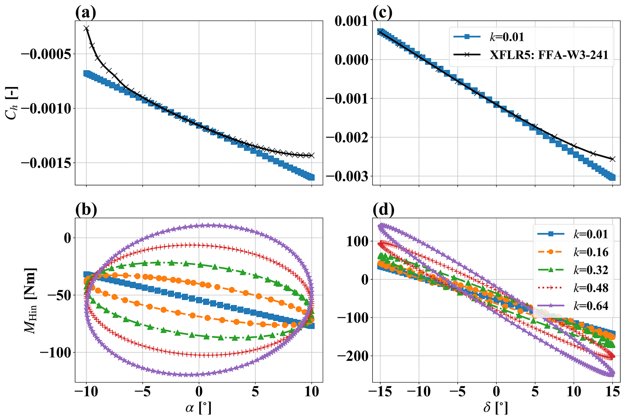
Figure 3 (a) C_h vs. α with δ=0^∘ from XFLR5 results and from quasi-steady model simulations. (b) M_Hin vs. α for several reduced freqs. k and δ=0^∘. (c) C_h vs. δ with α=0^∘ from XFLR5 results and from quasi-steady model simulations. (d) M_Hin vs. δ for several reduced freqs. k and α=0^∘.

Figure 3b and d show the modeled hinge moment M_Hin of a 3 m flapped blade section with 2 m chord length and a mass m_flap of 22.6 g. For these subfigures a relative wind speed V_rel of 80 m s⁻¹ is used, and it is assumed that the flapped blade section is at a rotor azimuth angle φ of 0^∘. This way we have M_H-g=0 Nm. In Fig. 3b, M_Hin is plotted for oscillations of α at several reduced frequencies k with a constant flap angle δ=0^∘. Figure 3d shows M_Hin for oscillations of δ and a constant α=0^∘. In both cases, the unsteady aerodynamics are clearly seen for larger values of k. In Fig. 3d we can also see the increased effect of M_H-I on M_Hin for larger values of k.

We note that – although not shown in Fig. 3 – the aerodynamic hinge model presented in this section is also capable of calculating the hinge moment due to the section's normal displacement h. This includes the implicit calculation of the effective angle of attack which depends on α, $\dot{\mathit{\alpha }}$, $\dot{h}$ and V_rel (Leishman, 2006, p. 496). A less compact and more readable form of the aerodynamic hinge moment model can be found in Leishman (2006, 492–497).

3.2 Estimation of the effective angle of attack

We can use the model presented in the previous section to estimate the effective angle of attack of the blade section by means of a linear observer. The idea is to estimate the internal states of a system based on the measured inputs and outputs. If we cannot measure the quantities α, $\dot{\mathit{\alpha }}$ and $\ddot{\mathit{\alpha }}$ (because we would need an inflow sensor), we have to estimate them using the measured M_Hin and other available sensors.

In this study, we follow an approach used in Kracht et al. (2015). The observer model is comprised of three submodels: a nonlinear M_H-g model, a linear hinge model (that estimates ${\widehat{M}}_{\mathrm{H}\text{-}\mathrm{A}}$ and ${\widehat{M}}_{\mathrm{H}\text{-}\mathrm{I}}$) and a signal model. The latter is used to estimate the quantities we cannot measure. All three models are combined to produce an estimated hinge model ${\widehat{M}}_{\mathrm{Hin}}$. The estimation is then compared to the measured M_Hin, and the error is fed back to the states of the linear hinge model and the signal model using an appropriately chosen gain L.

Figure 4 shows a graphical representation of the observer structure. The hinge moment model of the observer uses the same state-space matrices A_Hin, B_Hin, C_Hin and D_Hin, with the exception of D_Hin. The inertial loads given by Eq. (3) are included in the feedthrough term $D_{\ddot{\mathit{\delta }}}$ of D_Hin so that the linear observer can use the state-space matrices to estimate ${\widehat{M}}_{\mathrm{H}\text{-}\mathrm{A}}+{\widehat{M}}_{\mathrm{H}\text{-}\mathrm{I}}$ directly.

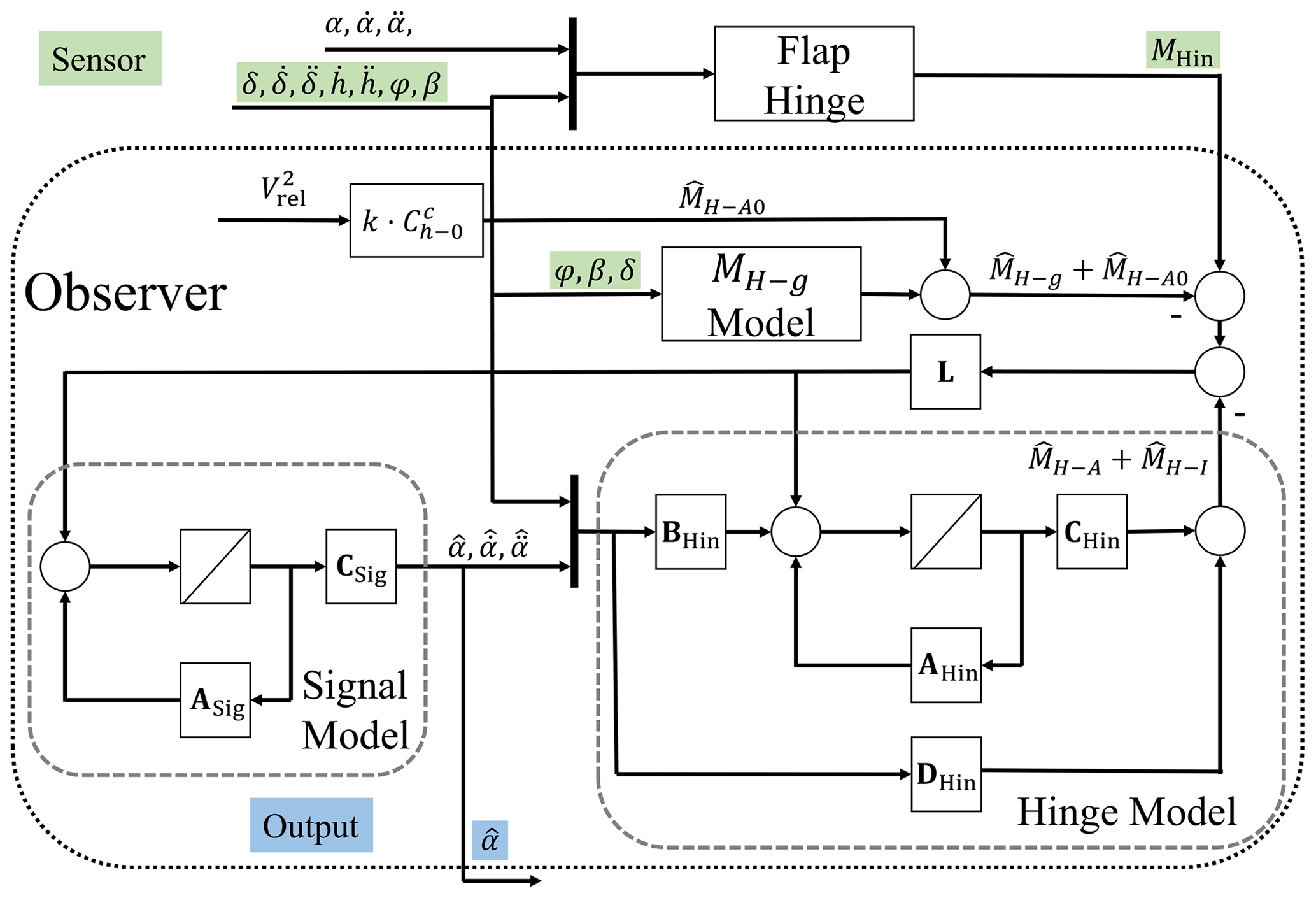
Figure 4 Representation of the linear observer for a constant V_rel. The required sensors and the observer output are marked with a green and blue background, respectively.

The output of the state-space representation does not include ${\widehat{M}}_{\mathrm{H}\text{-}\mathrm{A}\mathrm{0}}$, the constant value of the hinge moment for α=0^∘. In addition, M_H-g cannot be written in state-space form due to its non-linear nature. It therefore cannot be directly included in the observer model. However, it is highly deterministic and can be estimated using Eq. (2) with readily available sensors. The observer uses Eq. (2) to estimate ${\widehat{M}}_{\mathrm{H}\text{-}\mathrm{g}}$. As for ${\widehat{M}}_{\mathrm{H}\text{-}\mathrm{A}\mathrm{0}}$, the observer multiplies $V_{\mathrm{rel}}^{\mathrm{2}}$ by a constant factor that includes $C_{\mathrm{h}\text{-}\mathrm{0}}^{\mathrm{c}}$ and the dimensions of the blade section. Both quantities are subtracted from the measured M_Hin so that the error is calculated between (M_H-A+M_H-I) and (${\widehat{M}}_{\mathrm{H}\text{-}\mathrm{A}}+{\widehat{M}}_{\mathrm{H}\text{-}\mathrm{I}}$).

For this study we use a simple signal model. It basically assumes that α and its derivatives do not change with time. The choice of this signal model is based on the fact that the source of change of α – the incoming wind speed V_OP – is turbulent and therefore difficult to predict. The downside is that the estimated signal will always have a lag compared to the actual signal. The signal model has the following state-space matrices:

$$\begin{array}{}\text{(14)}& {\displaystyle }& {\displaystyle }{\mathbf{A}}_{\mathrm{Sig}}=\left[\begin{array}{ccc}\mathrm{0}& \mathrm{1}& \mathrm{0}\\ \mathrm{0}& \mathrm{0}& \mathrm{1}\\ \mathrm{0}& \mathrm{0}& \mathrm{0}\end{array}\right],\text{(15)}& {\displaystyle }& {\displaystyle }{\mathbf{C}}_{\mathrm{Sig}}={\mathbf{I}}_{\mathrm{3}\times \mathrm{3}}.\end{array}$$

We note that other signal models can be used, such as, e.g., a bank of independent harmonic oscillators (Kracht et al., 2015), if the wind conditions for a particular site are known with a certain degree of accuracy.

If we combine the signal and hinge moment models, we get a state space whose input vector is ${\mathit{u}}_{\mathrm{S}+\mathrm{H}}={\left(\begin{array}{ccccc}\mathit{\delta }& \dot{\mathit{\delta }}& \ddot{\mathit{\delta }}& \dot{h}& \ddot{h}\end{array}\right)}^T$ and its output is $y_{\mathrm{S}+\mathrm{H}}=({\widehat{M}}_{\mathrm{H}\text{-}\mathrm{A}}+{\widehat{M}}_{\mathrm{H}\text{-}\mathrm{I}})$. The state-space matrices for this combined system are as follows.

$$\begin{array}{}\text{(16)}& {\displaystyle }& {\displaystyle }{\mathbf{A}}_{\mathrm{S}+\mathrm{H}}=\left[\begin{array}{cc}{\mathbf{A}}_{\mathrm{Sig}}& {\mathbf{0}}_{\mathrm{3}\times \mathrm{4}}\\ {\mathbf{B}}_{\mathrm{Hin}}^{\mathit{\alpha }}& {\mathbf{A}}_{\mathrm{Hin}}\end{array}\right]\text{(17)}& {\displaystyle }& {\displaystyle }{\mathbf{B}}_{\mathrm{S}+\mathrm{H}}=\left[\begin{array}{c}{\mathbf{0}}_{\mathrm{3}\times \mathrm{5}}\\ {\mathbf{B}}_{\mathrm{Hin}}^{\mathrm{Res}}\end{array}\right]\text{(18)}& {\displaystyle }& {\displaystyle }{\mathbf{C}}_{\mathrm{S}+\mathrm{H}}=\left[\begin{array}{cccc}{D}_{\mathit{\alpha }}& D_{\dot{\mathit{\alpha }}}& D_{\ddot{\mathit{\alpha }}}& {\mathbf{C}}_{\mathrm{Hin}}\end{array}\right]\text{(19)}& {\displaystyle }& {\displaystyle }{\mathbf{D}}_{\mathrm{S}+\mathrm{H}}=\left[\begin{array}{ccccc}{D}_{\mathit{\delta }}& D_{\dot{\mathit{\delta }}}& D_{\ddot{\mathit{\delta }}}& D_{\dot{h}}& D_{\ddot{h}}\end{array}\right]\end{array}$$

In these equations, ${\mathbf{B}}_{\mathrm{Hin}}^{\mathit{\alpha }}$ corresponds to the sub-matrix of B_Hin that relates to α and its derivatives. ${\mathbf{B}}_{\mathrm{Hin}}^{\mathrm{Res}}$ corresponds to the rest of B_Hin. The entries of these matrices are written out explicitly in Appendix A.

The final state-space representation of our observer has the form

$$\begin{array}{}\text{(20)}& {\displaystyle }& {\displaystyle }{\mathbf{A}}_{\mathrm{obs}}={\mathbf{A}}_{\mathrm{S}+\mathrm{H}}-{\mathbf{LC}}_{\mathrm{S}+\mathrm{H}},\text{(21)}& {\displaystyle }& {\displaystyle }{\mathbf{B}}_{\mathrm{obs}}=\left[\begin{array}{cc}\left({\mathbf{B}}_{\mathrm{S}+\mathrm{H}}-{\mathbf{LD}}_{\mathrm{S}+\mathrm{H}}\right)& \mathbf{L}\end{array}\right],\text{(22)}& {\displaystyle }& {\displaystyle }{\mathbf{C}}_{\mathrm{obs}}=\left[\begin{array}{ccccccc}\mathrm{1}& \mathrm{0}& \mathrm{0}& \mathrm{0}& \mathrm{0}& \mathrm{0}& \mathrm{0}\end{array}\right],\text{(23)}& {\displaystyle }& {\displaystyle }{\mathbf{D}}_{\mathrm{obs}}={\mathbf{0}}_{\mathrm{1}\times \mathrm{6}}.\end{array}$$

Its input vector is given by ${\mathit{u}}_{\mathrm{obs}}={\left(\begin{array}{cccccc}\mathit{\delta }& \dot{\mathit{\delta }}& \ddot{\mathit{\delta }}& \dot{h}& \ddot{h}& \left(M_{\mathrm{Hin}}-{\widehat{M}}_{\mathrm{H}\text{-}\mathrm{g}}-{\widehat{M}}_{\mathrm{H}\text{-}\mathrm{A}\mathrm{0}}\right)\end{array}\right)}^T$ and its output is $y_{\mathrm{obs}}=\widehat{\mathit{\alpha }}$.

The gain matrix L is obtained using a standard Kalman filter design. In order to tune our estimator, we use the covariance matrices for process noise Q_L and for measurement noise R_L.

The derivation of the linear estimator above is only valid for one fixed value of V_rel. This is not the case for a wind turbine blade in normal operation. In order to extend the estimator so that it can be used for varying V_rel, a linear parameter varying (LPV) model was built using the observer matrices for different values of V_rel. This way, the nonlinear aerodynamic behavior of the flap hinge moment is parameterized with a set of linear observers, allowing for a fast and optimal estimation for each value of V_rel. If V_rel is used for the LPV model, it needs to be measured or estimated. The former option is not available, since we chose not to use inflow sensors. This leaves us with the estimation option, presented in the next section.

3.3 Estimation of the relative velocity

To estimate V_rel, we decompose the velocity into in-plane and out-of-plane components. The in-plane component of the rigid blade can be readily estimated using the rotor speed Ω and the distance between the hub center and spanwise center of the flapped blade section r_flap:

$$\begin{array}{}\text{(24)}& V_{\mathrm{IP}}=\mathrm{\Omega }\cdot r_{\mathrm{flap}}.\end{array}$$

For the out-of-plane component, we use a simple estimator based on the anemometer wind speed V_Ane, the rotor azimuth angle φ and the normal velocities of the flapped blade sections of the three blades that share the same spanwise distance from the rotor hub (${\dot{h}}_{\mathrm{1}}$–${\dot{h}}_{\mathrm{3}}$). The latter can be obtained by integrating the signal of accelerometers measuring the local accelerations of the sections of each blade:

$$\begin{array}{}\text{(25)}& V_{\mathrm{OP}}=V_{\mathrm{Ane}}+{\mathrm{\Delta }}_{\mathrm{Vop}}\left({\dot{h}}_{\mathrm{1}},{\dot{h}}_{\mathrm{2}},{\dot{h}}_{\mathrm{3}},\mathit{\phi }\right).\end{array}$$

${\mathrm{\Delta }}_{\mathrm{Vop}}({\dot{h}}_{\mathrm{1}}$, ${\dot{h}}_{\mathrm{2}}$, ${\dot{h}}_{\mathrm{3}}$, φ) is a function that accounts for the vertical variation in V_OP dependent on the azimuthal position of the blade due to, e.g., wind shear. It comprises two parts: a vertical variation part and a tower shadow model.

The vertical variation part uses the once-per-revolution Coleman transform of the velocities of the blade sections normal to the chord to get an equivalent amplitude of the vertically varying velocity normal to the chord of the rotor annulus at the spanwise position of the flapped blade section.

$$\begin{array}{}\text{(26)}& \begin{array}{rl}{v}_{\sin }& ={\displaystyle \frac{\mathrm{2}}{\mathrm{3}}}\cdot \left(\sin \left(\mathit{\phi }\right)\cdot {\dot{h}}_{\mathrm{1}}+\sin \left(\mathit{\phi }+{\displaystyle \frac{\mathrm{2}\mathit{\pi }}{\mathrm{3}}}\right)\cdot {\dot{h}}_{\mathrm{2}}\right.\\ & \left.+\sin \left(\mathit{\phi }+{\displaystyle \frac{\mathrm{4}\mathit{\pi }}{\mathrm{3}}}\right)\cdot {\dot{h}}_{\mathrm{3}}\right)\end{array}\end{array}$$

We then use a linear transform of this quantity to estimate the vertical variation in the out-of-plane wind velocity at different azimuthal positions of the blade.

$$\begin{array}{}\text{(27)}& {\mathrm{\Delta }}_{\mathrm{Vop}\text{-}\mathrm{v}}=\left\{\begin{array}{cl}{c}_{\mathrm{1}}\cdot \cos \left(\mathit{\phi }\right)\cdot v_{\sin }+c_{\mathrm{2}}& \mathrm{for}-\frac{\mathit{\pi }}{\mathrm{2}}\le \mathit{\phi }\le \frac{\mathit{\pi }}{\mathrm{2}}\\ c_{\mathrm{3}}\cdot \cos \left(\mathit{\phi }\right)\cdot v_{\sin }+c_{\mathrm{4}}& \mathrm{for}\frac{\mathit{\pi }}{\mathrm{2}}<\mathit{\phi }<\frac{\mathrm{3}\mathit{\pi }}{\mathrm{2}}\end{array}\right.\end{array}$$

The two cases in the above equation are necessary because of the non-linear effect of wind shear on the vertical wind velocity. Because we are approximating the out-of-plane variation with a simple cosine function, we use two amplitudes to account for the variation at the lower and upper half planes of the rotor. The constants c₁–c₄ were obtained by fitting the results of the values of Δ_Vop-v and v_sin from aeroelastic constant wind simulations of the turbine. In addition, v_sin is low-passed and notch filtered to filter out the higher-frequency contributions to the normal velocity of the rotor annulus.

The tower shadow variation part uses a simplified approximation of the tower shadow model from Bak et al. (2001). We simplified this model by assuming a constant x distance (out of plane) between blade and tower. It was taken as the average distance between the blade section and the tower surface in constant wind aeroelastic simulations. That is one constant value that is used for all wind speeds. The tower shadow variation is added to Δ_Vop-v to get Δ_Vop.

Once we have calculated V_IP and V_OP, we use both quantities to obtain the relative velocity of the flapped blade section. In uniform aligned inflow, V_rel would be the resulting velocity from the previous quantities. This is almost never the case. To account for the oblique inflow, we use the trigonometric correction presented in Damiani et al. (2018):

$$\begin{array}{}\text{(28)}& \begin{array}{rl}{V}_{\mathrm{rel}}& =\left({\left(V_{\mathrm{OP}}\cdot \cos \left(\mathit{\gamma }\right)\cdot \cos \left(\mathit{\tau }\right)-\dot{x}\right)}^{\mathrm{2}}+\left(V_{\mathrm{IP}}-\dot{y}-V_{\mathrm{OP}}\right.\right.\\ & {\left.{\left.\cdot \left(\cos \right(\mathit{\gamma })\cdot \sin (\mathit{\tau })\cdot \sin (\mathit{\phi })+\sin (\mathit{\gamma })\cdot \cos (\mathit{\phi }\left)\right)\right)}^{\mathrm{2}}\right)}^{\frac{\mathrm{1}}{\mathrm{2}}}.\end{array}\end{array}$$

For this correction, we need to know the shaft tilt angle τ and the current yaw-misalignment angle γ. The latter can be obtained via the hub-mounted anemometers. In Eq. (28), we also included the in-plane ($\dot{y}$) and out-of-plane ($\dot{x}$) velocities of the flapped blade section due to blade elasticity. These can be obtained by rotating the chordwise and normal velocities of the section by the current blade pitch angle and the twist angle (see Fig. 2):

$$\begin{array}{}\text{(29)}& {\displaystyle }& {\displaystyle }\dot{x}=\dot{h}\cdot \cos (\mathrm{180}{}^{\circ }-(\mathit{\beta }+\mathit{\theta }\left)\right)+\dot{f}\cdot \sin (\mathrm{180}{}^{\circ }-(\mathit{\beta }+\mathit{\theta }\left)\right),\text{(30)}& {\displaystyle }& {\displaystyle }\dot{y}=-\dot{h}\cdot \sin (\mathrm{180}{}^{\circ }-(\mathit{\beta }+\mathit{\theta }\left)\right)+\dot{f}\cdot \cos (\mathrm{180}{}^{\circ }-(\mathit{\beta }+\mathit{\theta }\left)\right).\end{array}$$

We note that the expression for V_OP is a relative simple estimation of the out-of-plane velocity. This is not exact since there is significant variation in V_OP along the rotor disc due to the non-linear wind shear and turbulence. This error can be tolerated because $V_{\mathrm{IP}}^{\mathrm{2}}$ dominates in the right-hand side of Eq. (28). This is specially so for large rotor blades with high tip speed ratios, which is the current industry trend. So an error in V_OP will only have a small contribution towards V_rel and hence towards $\widehat{\mathit{\alpha }}$. There have been several studies that include more accurate estimations of the rotor effective wind speed, Simley and Pao (2016) and Bertelè et al. (2017) being two examples. Such methods could be used to further increase the accuracy of the current wind speed estimator. Additional improvements could also be achieved if we include the effect of tower top displacements on the estimated local V_rel.

Combining the V_rel estimator with the estimator for α gives us the final LPV observer based on the flap hinge moment sensor.

3.4 Discussion

The derivation of the model and observer presented in this section is based on several assumptions. The first is the 2D airfoil analysis assumption. It is therefore only correct for an infinitely thin blade station. Changes in the wind distribution and angle of attack along the span of the blade section will have an integrated effect on the hinge moment and potentially deviate from the pure 2D analysis. In this study we assume that the aerodynamic conditions do not change significantly within a flapped blade section and therefore can be treated as effective quantities for the section.

To have an idea of the error made with this assumption, we take the innermost 3 m flapped section with the aforementioned sensors located at the center of the section span. The center of this section is situated at a blade radius of 65.5 m. For turbine operation at rated rotor speed, the difference of local in-plane wind speeds between the center of the blade section and the inner part of the section span is about 2 % of the in-plane velocity at the section center. For the outer flapped sections, the relative error decreases due to the increased wind speed used for reference. For the out-of-plane wind speed we can estimate the error by looking at the coherence function of the spatial distribution of the turbulence. Assuming a Kaimal wind model, the spatial coherence function of two points that are 1.5 m apart is 0.75 for a frequency corresponding to 1P and an average out-of-plane velocity of 10 m s⁻¹ (IEC 61400-1 Ed. 3, 2005).

Ultimately the validity of this assumption is reflected in the controller performance and has to be assessed experimentally or in simulations. Jones et al. (2018) also assume a correlation between the lift forces occurring at nearby blade stations and the lift force of the blade station where a pitot tube is installed. With this assumption they are able to enhance the performance of an IPC controller based on the information of one inflow sensor per blade. In Barlas et al. (2018), the authors successfully control a 2 m flapped blade section using a feed-forward controller based on the local information of one pitot tube. These are encouraging results suggesting the aforementioned assumption is valid.

The observer presented in this section is based on a thin airfoil model and does not correspond to physical airfoils used in wind turbines. As we saw in Sect. 3.1.2, our model only partially captures the viscous effects of flow separation that greatly influence the behavior of C_h as a function of α. We approximated this effect with the use of flap effectiveness coefficients. Nonetheless, the nonlinear behavior for larger absolute values of α was not captured. To improve our modeling, we could determine the complete state-space models of the flap hinge moment at different wind speeds experimentally. This could be done for example in wind tunnel tests with the help of system identification techniques (Bartholomay et al., 2018).

4 Estimator performance

In this section we present the performance of the estimator using a series of steady and turbulent wind fields in combination with the turbine model. To illustrate the performance of our estimator, we simulate one 3 m flapped blade section at the rotor spanwise position of 74.3 m. The flap angle is held constant at δ=0^∘ for all the simulations in this section.

4.1 Implementation of model and observer in the aeroelastic codes

Both the hinge moment model and the observer are included in the TUB Controller (Perez-Becker et al., 2021). The inputs for the model ($\mathit{u}={\left(\begin{array}{cccccccc}\mathit{\alpha }& \dot{\mathit{\alpha }}& \ddot{\mathit{\alpha }}& \mathit{\delta }& \dot{\mathit{\delta }}& \ddot{\mathit{\delta }}& \dot{h}& \ddot{h}\end{array}\right)}^T$ and V_rel) and for the observer (${\mathit{u}}_{\mathrm{S}+\mathrm{H}}={\left(\begin{array}{ccccc}\mathit{\delta }& \dot{\mathit{\delta }}& \ddot{\mathit{\delta }}& \dot{h}& \ddot{h}\end{array}\right)}^T$ and the inputs for the velocity estimator) are calculated by the aeroelastic code and passed to the controller via an appropriate interface. For the FAST simulations the interface occurred within a Simulink environment. For the QBlade simulations, a special interface was developed between the software and the controller to be able to pass the required inputs.

As discussed in Sect. 3.4, the hinge moment model and observer are inherently 2D models that require the input at one specific location. We chose this location to be the center of each flapped blade section and assume that this location is representative for the whole section. For the FAST simulations, the blade is discretized into 46 aerodynamic and 57 structural nodes, with nodes specially chosen at the center of each flapped blade section. In QBlade, the blade is discretized into 25 aerodynamic and 20 structural nodes. The aerodynamic nodes are spaced sinusoidally along the blade span. The aerodynamic and structural information at the center of the flapped blade sections is obtained by linearly interpolating the information from neighboring nodes.

The performance of our observer is evaluated by its ability to estimate the representative aerodynamic quantities at the center of each flapped blade section.

This modeling approach could be improved if we consider more aerodynamic blade elements so that several of them lie within a flapped blade section. These elements would be used to calculate the lift force acting on the whole section. Using a representative airfoil polar for the blade section, we could calculate the effective angle of attack at the center location of the section and use this as an input for our hinge model. It would also be this effective angle of attack that would be estimated by our observer.

4.2 Steady wind conditions

The parameters of the steady wind simulations are listed in Table 1 under the column “Steady calculations”.

Table 1 Simulation parameters for aeroelastic calculations.

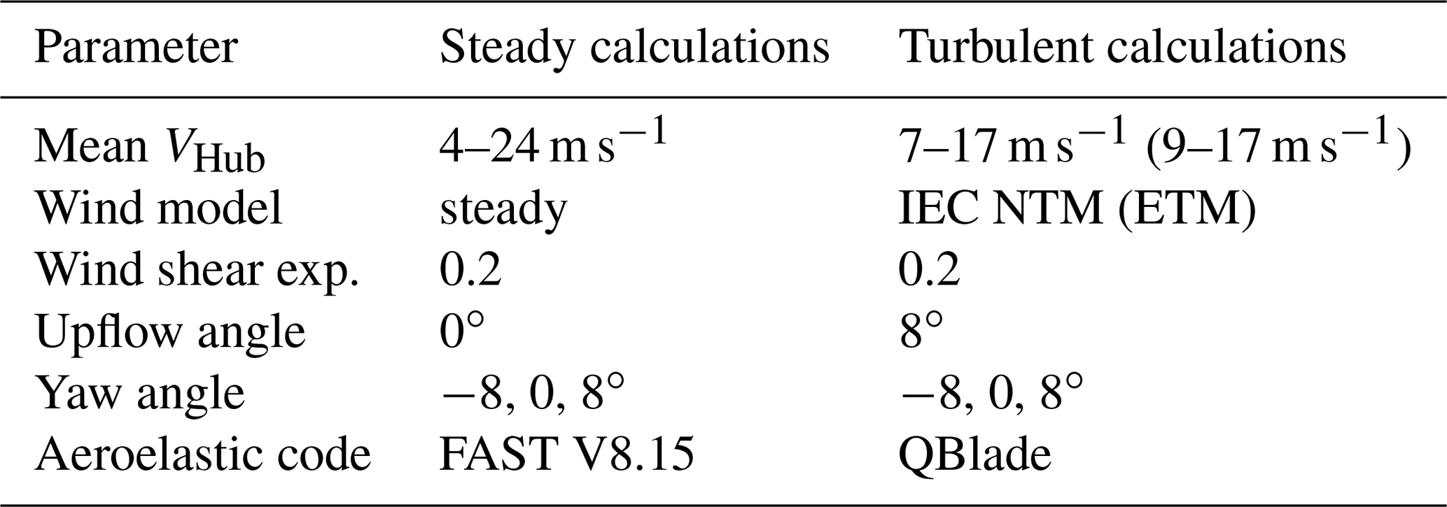
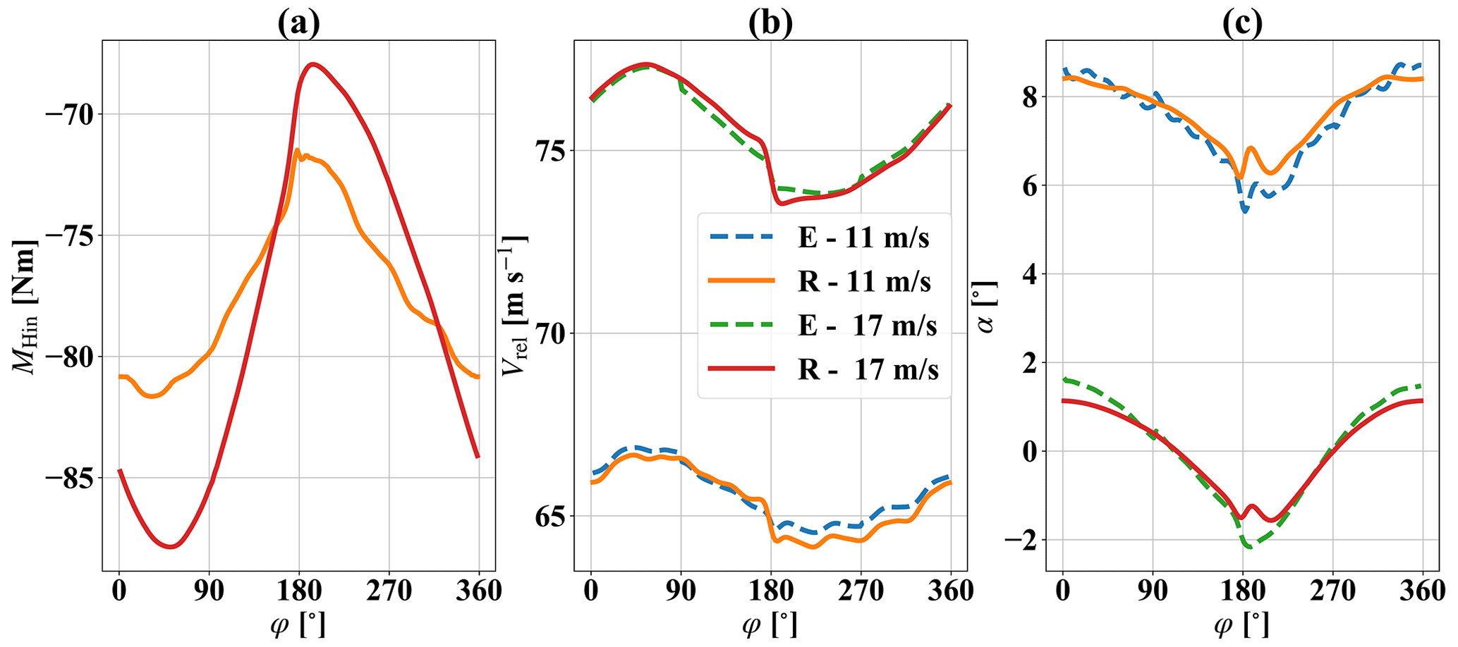
Figure 5 Behavior of the estimator for two different wind speeds as a function of the rotor azimuth angle. (a) Flap hinge moment; (b) relative velocity; (c) angle of attack. E: estimated; R: real.

Figure 5 shows three key variables for our estimator in simulations with two different hub height wind speeds. One wind speed around rated wind and one above rated where the influence of the pitch angle increases. The simulations were performed with steady wind speeds and a constant nacelle yaw angle of −8^∘. We can see in Fig. 5a the behavior of M_Hin as a function of φ. In both the 11 and the 17 m s⁻¹ wind speed simulations M_Hin is mostly determined by M_H-A. The larger azimuthal variation in M_Hin in the 17 m s⁻¹ wind speed simulations comes from the higher relative wind speed variations due to wind shear.

Figure 5b and c show the estimated and real values of V_rel and α as a function of φ. We can see that the observer is able to estimate the relative velocity and angle of attack at this blade section well. There is a slight delay of $\widehat{\mathit{\alpha }}$ compared to α, but it is small at the timescale of one rotor revolution. For both wind speeds, there is a clear difference at an azimuth angle of φ=180^∘. The velocity drop of V_rel is due to the tower shadow, which was only approximated in our velocity estimator. This tower shadow effect on α is also not captured correctly by our estimator (Fig. 5c). We can also see in these figures the variation due to wind shear of V_rel and α. Our approximation captures this variation well but there are still some small differences between the real and the estimated quantities.

Figure 6 shows the results of steady wind calculations for all wind speeds relevant to power production and for three different yaw angles of the nacelle. The markers represent the mean of the steady simulations, and the error bars represent the extrema of the simulations. Figure 6a, c and e show the estimated and real relative velocities at the blade section. Our velocity estimator is able to capture these differences and keeps the relative error of the mean velocities at below 0.4 %.

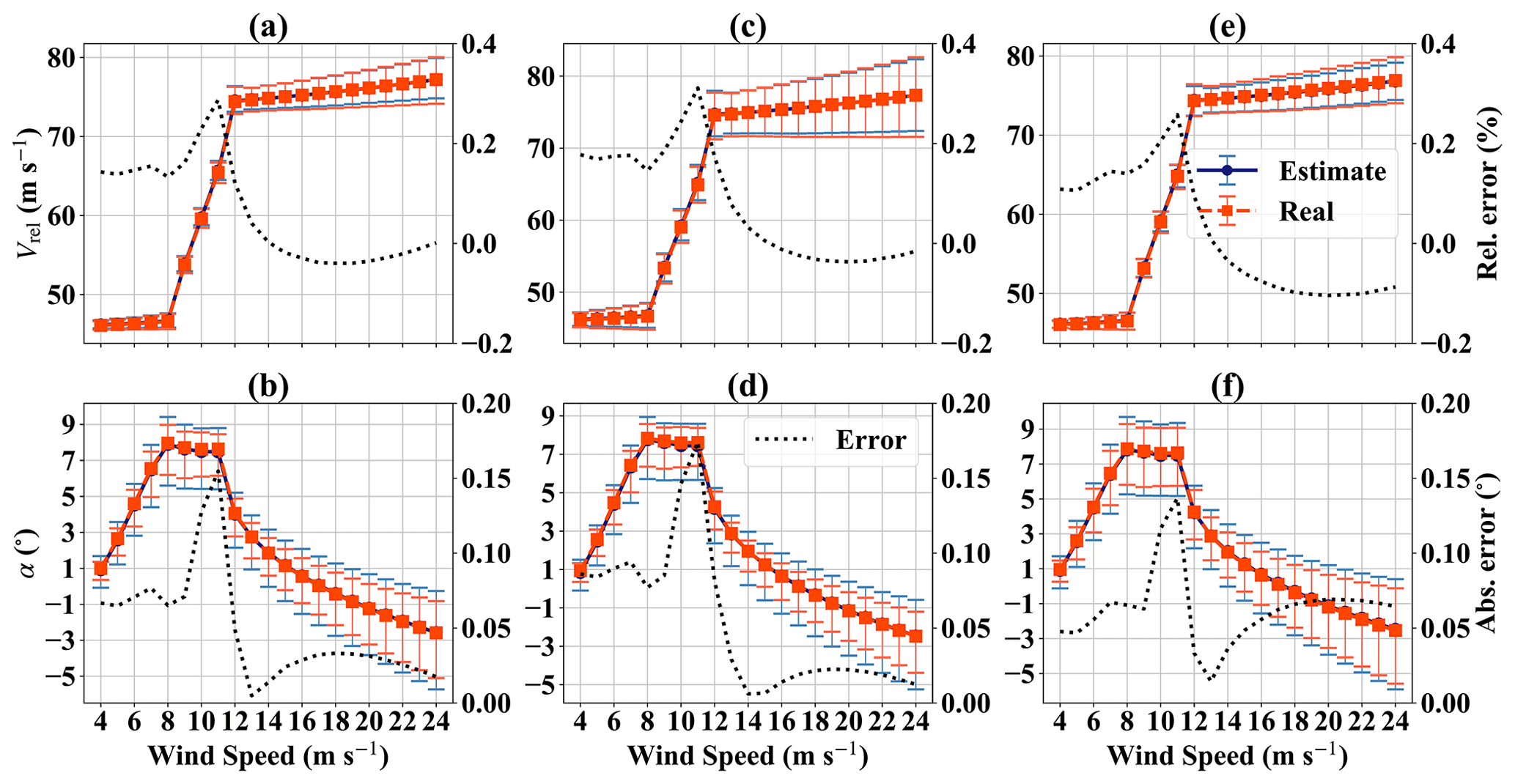
Figure 6 Observer performance for steady-state calculations. (a) V_rel vs. V_hub for 0^∘ yaw simulations; (b) α vs. V_hub for 0^∘ yaw simulations; (c) V_rel vs. V_hub for 8^∘ yaw simulations; (d) α vs. V_hub for 8^∘ yaw simulations; (e) V_rel vs. V_hub for −8^∘ yaw simulations; (f) α vs. V_hub for −8^∘ yaw simulations.

Figure 6b, d and f show the corresponding estimated and real values of α at the blade section. We see that the observer manages to estimate the mean angle of attack with an error below 0.2^∘ for all simulations. The differences in the extrema of α are more marked, especially for higher values of V_hub. The differences in the minima can be explained by the approximation of the tower shadow, which fails to capture the dip in α at azimuth values of φ=180^∘ (Fig. 5c). If we look at the range of V_hub between 8 and 14 m s⁻¹, we can see that the differences between real and estimated maxima of α are small. This is of importance if we want to use the observer as part of a load alleviation controller targeting extreme loads. This is the wind speed range where the turbine sees the highest out-of-plane loading in power production (Barlas et al., 2016b).

4.3 Turbulent wind conditions

We also analyzed the performance of our estimator in fully turbulent wind load calculations. These situations are especially challenging for the observer because our relative velocity estimator does not model turbulent out-of-plane wind speeds. The setup for the turbulent calculations is shown in Table 1 in the column “Turbulent calculations”.

Because the observer lacks the turbulent variation in the out-of-plane wind speed in the relative velocity estimator, the estimated $\widehat{\mathit{\alpha }}$ will have a significantly larger variation than the actual α. This is because the observer will attribute the changes in M_Hin to the unmeasured α, since it can only assume a correct parametrization coming from ${\widehat{V}}_{\mathrm{rel}}$. In order to limit the variations in $\widehat{\mathit{\alpha }}$, an additional first-order low-pass filter was added to the output of the $\widehat{\mathit{\alpha }}$ observer.

Figure 7 shows time series that illustrate the performance of the observer in turbulent wind conditions. The simulations are for mean V_hub values of 7 and 15 m s⁻¹, representing scenarios below and above rated wind conditions. The simulations were done using the IEC NTM turbulent wind model.

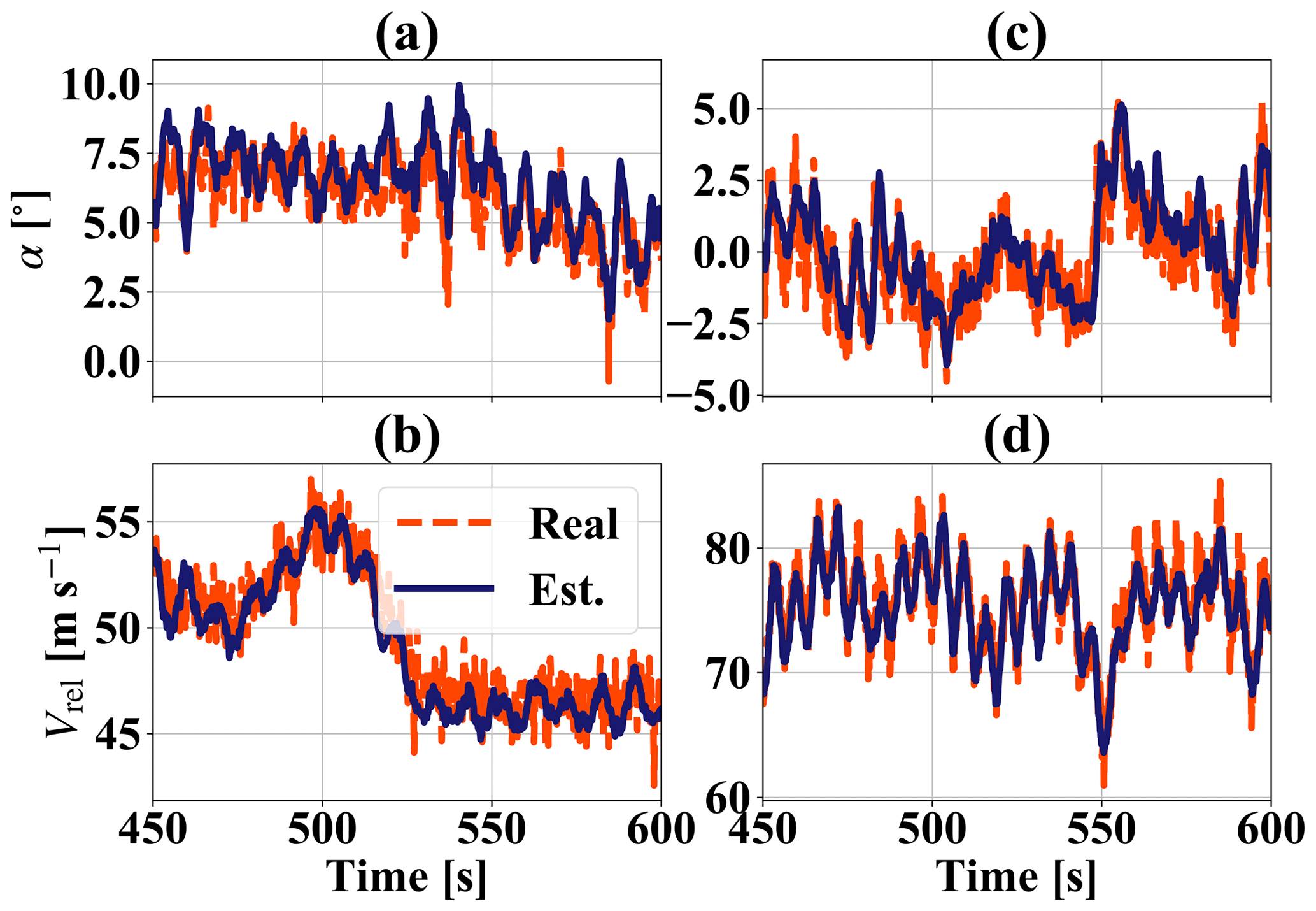
Figure 7 Time series of the estimator performance for two different turbulent wind speed simulations. (a) α for V_hub=7 m s⁻¹; (b) V_rel for V_hub=7 m s⁻¹; (c) α for V_hub=15 m s⁻¹; (d) V_rel for V_hub=15 m s⁻¹.

We can see in Fig. 7 that the estimator is able to capture the low-frequency variation in α and V_rel well. The differences arise from the effect of the turbulent wind speed. Depending on the wind speed, the magnitude of the differences between ${\widehat{V}}_{\mathrm{rel}}$ and V_rel can be small or large. Figure 7b shows the example of 7 m s⁻¹ mean V_hub simulations where the differences between ${\widehat{V}}_{\mathrm{rel}}$ and V_rel are small. The differences can also be more significant, especially for larger wind speeds. In the 15 m s⁻¹ example (Fig. 7d), we can see large differences in the 1P variation in V_rel in the simulation time between 550 and 600 s. These variations arise from the repeated passing of the rotating blade through large-scale, slowly varying turbulent wind gusts and hence are not accounted for in ${\widehat{V}}_{\mathrm{rel}}$. Due to the low-pass filtering of $\widehat{\mathit{\alpha }}$, the abovementioned differences in V_rel do not lead to large oscillations of the former, and we can see that $\widehat{\mathit{\alpha }}$ follows α well in the low-frequency regime.

The filtering introduces a time lag which could potentially be detrimental for a controller. The effects of the filter would certainly be more marked for an extreme load controller than for a fatigue load controller. Since we are interested in the extreme load reduction potential of flaps, we will be analyzing the more critical situation in this study. The description and performance of such an extreme loads controller are presented in the next section.

The estimated ${\widehat{V}}_{\mathrm{rel}}$ and $\widehat{\mathit{\alpha }}$ from the observer can also be used for a pitch-based fatigue load controller – such as the one presented by Jones et al. (2018) – thereby indirectly increasing the use of the flap system beyond extreme load reduction.

5 Extreme load reduction under turbulent conditions

In this section we integrate the estimator presented in Sect. 3 in a simple flap extreme load controller and use it to reduce extreme blade loads and deflections.

5.1 Extreme load controller

The controller used in this study is based on the extreme load controller presented by Barlas et al. (2016b). It has an attractively simple architecture and was shown to work effectively in the mentioned study. In the original controller, all three out-of-plane BRBM signals $M_{Y\text{-}i}^{\mathrm{BR}}$ are compared to a maximum threshold M_thr. If

$$\begin{array}{}\text{(31)}& M_{Y\text{-}i}^{\mathrm{BR}}\ge M_{\mathrm{thr}},\end{array}$$

then all flaps of all blades are deployed to a target angle.

We expanded this controller by including additional sensors and criteria to trigger flap action. The controller logic is shown in Fig. 8. The subscripts of the figure correspond to the jth flap of the ith blade. Although there are six flaps per blade, the controller treats them all as a single unit. The input of the individual flaps is averaged per blade (denoted by the symbol $\stackrel{\mathrm{‾}}{(\cdot )}$). Combinations of input sensors are compared against thresholds. If they pass the thresholds, then all flaps of all blades are set to a target value. The first condition for triggering the flap action is Eq. (31). This condition is identical to the one proposed by Barlas et al. (2016b). Here, a careful selection of M_thr has to be made in order not to influence the turbine in normal power production. The other three conditions are

$$\begin{array}{}\text{(32)}& {\displaystyle }& {\displaystyle }\left(M_{Y\text{-}i}^{\mathrm{BR}}\ge M_{\mathrm{tr}\mathrm{1}}\mathrm{and}{\stackrel{\mathrm{‾}}{\dot{x}}}_i\ge {\dot{x}}_{\mathrm{tr}\mathrm{1}}\right)\mathrm{or}\left(M_{Y\text{-}i}^{\mathrm{BR}}\ge M_{\mathrm{tr}\mathrm{2}}\mathrm{and}{\stackrel{\mathrm{‾}}{\dot{x}}}_i\ge {\dot{x}}_{\mathrm{tr}\mathrm{2}}\right),\text{(33)}& {\displaystyle }& {\displaystyle }\left(M_{Y\text{-}i}^{\mathrm{BR}}\ge M_{\mathrm{tr}\mathrm{1}}\mathrm{and}{\stackrel{\mathrm{‾}}{\widehat{\mathit{\alpha }}}}_i\ge {\mathit{\alpha }}_{\mathrm{tr}\mathrm{1}}\mathrm{and}{\stackrel{\mathrm{‾}}{\widehat{V}}}_{\mathrm{rel}\text{-}i}\ge V_{\mathrm{tr}\mathrm{1}}\right),\text{(34)}& {\displaystyle }& {\displaystyle }\left(M_{Y\text{-}i}^{\mathrm{BR}}\ge M_{\mathrm{tr}\mathrm{1}}\mathrm{and}{\stackrel{\mathrm{‾}}{M}}_{\mathrm{Hin}\text{-}i}\le M_{\mathrm{Hin}\text{-}\mathrm{tr}\mathrm{1}}\mathrm{and}{\stackrel{\mathrm{‾}}{\widehat{V}}}_{\mathrm{rel}\text{-}i}\ge V_{\mathrm{tr}\mathrm{1}}\right).\end{array}$$

Here, M_tr-i, ${\dot{x}}_{\mathrm{tr}\text{-}i}$, α_tr1, V_tr1 and M_Hin-tr1 are threshold values for the respective input sensors. The idea of these conditions is to lower the threshold for $M_{Y\text{-}i}^{\mathrm{BR}}$ to deploy the flaps for the cases where extreme bending moments are expected to happen. It was seen in preliminary simulations that the flap deployment had a delayed effect on the lowering of the blade root bending moment. Deploying the flaps close to a load peak would only have a small load reduction effect on $M_{Y\text{-}i}^{\mathrm{BR}}$. Yet this condition is necessary in order to limit the influence of the flap controller on the power output of the turbine.

Figure 8 Graphical representation of the controller logic. The conditions 1 to 4 are given by Eqs. (31) to (34).

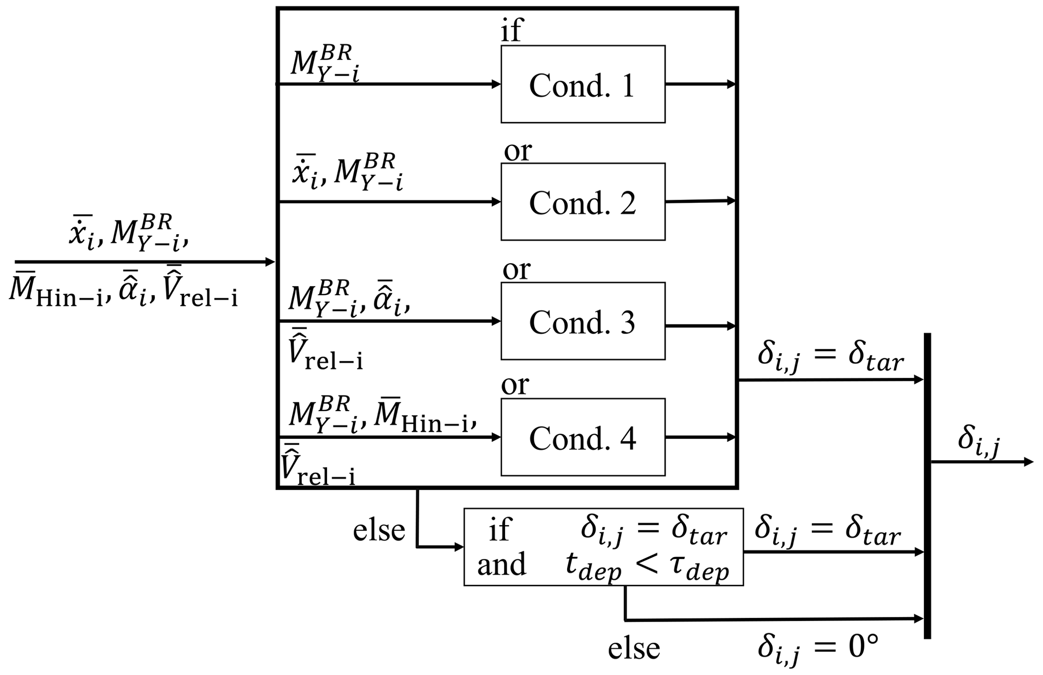
By using the flap hinge sensor in the outer blade span (Eqs. 33 and 34), the controller has additional aerodynamic information about the likelihood of a strong wind gust and is able to deploy the flaps at a lower threshold value of $M_{Y\text{-}i}^{\mathrm{BR}}$ (M_tr1<M_thr), thus giving the flaps more time to effectively mitigate the blade root loads. We mentioned in Sect. 4.3 that our observer includes a low-pass filter for $\widehat{\mathit{\alpha }}$ which causes a delay in the signal. To enable our controller to sense sudden increases in α, we also included a condition based on ${\stackrel{\mathrm{‾}}{M}}_{\mathrm{Hin}\text{-}i}$ directly. Assuming that the flap deployment angle will mostly be ${\mathit{\delta }}_{i,j}=\mathrm{0}$^∘, the value of ${\stackrel{\mathrm{‾}}{M}}_{\mathrm{Hin}\text{-}i}$ will be approximately proportional to ${\stackrel{\mathrm{‾}}{\mathit{\alpha }}}_i$ for small reduced frequencies (Fig. 3b).

Preliminary simulations also revealed that blade deflection dynamics are critical for predicting extreme events of $M_{Y\text{-}i}^{\mathrm{BR}}$ and were not always strongly correlated to the aerodynamic information. The controller includes Eq. (32) to account for extreme loads due to large values of $\stackrel{\mathrm{‾}}{\dot{x}}$. We include two conditions to also account for very high velocities that occur at lower values of $M_{Y\text{-}i}^{\mathrm{BR}}$ (M_tr2<M_tr1 and ${\dot{x}}_{\mathrm{tr}\mathrm{2}}>{\dot{x}}_{\mathrm{tr}\mathrm{1}}$).

If any of the above conditions are met for any blade, then all flaps of all blades are deployed to the target angle ${\mathit{\delta }}_{tar}=-\mathrm{14.5}$^∘. This value is slightly lower than the maximum modeled value in the polars. This was done to still be able to model the aerodynamic effect of a flap angle overshoot when the flaps are deployed. Additionally, the flaps were kept deployed for a given time τ_dep before they were returned to the original position. τ_dep was chosen to be about a third of one rotor period. This way if a localized gust triggers the flap controller of one blade, the following blade will already have deployed flaps when encountering the local gust. Finally, the controller also returns the flaps to their 0^∘ position with a reduced rate compared to the maximum flap rate. This is to have a smooth return to normal conditions and to avoid excessive oscillations of the blades by frequent on–off transitions.

The conditions explained so far are valid for cases where the strategy is used to mitigate the maxima of $M_{Y\text{-}i}^{\mathrm{BR}}$. This is the case of the considered load cases (Table 1). Equivalent conditions can be defined for the controller to mitigate the minima of $M_{Y\text{-}i}^{\mathrm{BR}}$.

We note that this controller treats all flaps in one blade as a single unit. Why should we make the additional effort to include multiple flaps per blade? One reason for having several flaps per blade instead of one is that a system of multiple independent flaps will still be able to reduce the loads in the event of one flap ceasing to function. This makes the system more redundant and thus more appropriate for extreme load reduction. A second reason is that the controller will have sensorial input from multiple sources. Averaging the signals of the six flaps smooths out possible local variations that could arise from using a single set of sensors. Finally, having multiple sensors and actuators per blade opens up the possibility of using local distributed control strategies in future studies.

5.2 Metrics

The metrics considered in this study are max($M_Y^{\mathrm{BR}}$) – the extreme out-of-plane bending moment at the blade root, max($M_{XY}^{\mathrm{BR}}$) – the extreme resulting bending moment at the blade root – and max($D_X^{\mathrm{T}\mathrm{2}\mathrm{T}}$) – the maximum blade out-of-plane deflection in the region defined by 5^∘ before the blade's closest azimuthal position to the tower and 5^∘ after this position. For a blade whose rotor azimuth angle is defined as 0^∘ when the blade is pointing vertically upward, this region would lie between the azimuth angles of 175 and 185^∘. This metric gives us an estimate of the minimum blade tip-to-tower surface distance.

Because we are dealing with stochastic wind simulations, we chose to follow the averaging procedure for extreme values described in IEC 61400-1 Ed. 3 (2005). The maximum value of $M_Y^{\mathrm{BR}}$, $M_{XY}^{\mathrm{BR}}$ and $D_X^{\mathrm{T}\mathrm{2}\mathrm{T}}$ (considering all three blades) is recorded for each simulation. The extreme value is then taken as the average of the six highest maxima of all simulations. For the case of $M_{XY}^{\mathrm{BR}}$, we did this averaging analysis for 72 different angular bins. For each time step, the direction of the load vector was calculated, and the maximum of $M_{XY}^{\mathrm{BR}}$ was determined for each angular bin in each simulation. This gives a more detailed picture of the effect of the flap controller on the extreme resulting bending moments in different load directions. No safety factors were applied since all the considered load cases share the same safety factor.

A complete analysis should include other key turbine sensors to measure the overall effect of the controller on the turbine. We chose not to include these sensors in order to limit the scope of this study.

5.3 Simulation setup

In this study we focused on the load case group that caused the highest $M_{XY}^{\mathrm{BR}}$ design loads of our selected turbine (Bak et al., 2013). This is the DLC load case group 1.3 which has the ETM wind model. We considered a subset of wind speed bins of this group around the rated wind speed (see Table 1 in the column “Turbulent calculations”). This is also the region of maximum rotor thrust and thus the expected maximum values of $M_{XY}^{\mathrm{BR}}$ and $D_X^{\mathrm{T}\mathrm{2}\mathrm{T}}$. We considered wind speeds in a range of mean V_Hub between 9 and 17 m s⁻¹ in 2 m s⁻¹ steps. Six different simulations were done for each wind speed bin, giving us a total of 30 simulations for each controller configuration. We also included the results of simulations from the DLC load case group 1.1 without flap controller. This way we have a reference of the load increase due to the increased turbulence of the DLC 1.3 group.

Although the number of simulations is rather low to determine the overall extreme values of $M_{XY}^{\mathrm{BR}}$ and $D_X^{\mathrm{T}\mathrm{2}\mathrm{T}}$, our selection will give us a good estimate of their maxima. By using QBlade – which has the lifting line free vortex wake (LLFVW) aerodynamic model and a multi-body based structural model – we ensure that the results of our load calculations are more accurate than with other codes that use the more common BEM aerodynamic model (Perez-Becker et al., 2020). In all simulations we included additional 100 s simulation time to allow the wake to develop. This time was discarded in our analysis.

5.4 Results

Figure 9 shows an overview of the maxima of $M_Y^{\mathrm{BR}}$ for the individual simulations of the different DLC groups and controller configurations.

Figure 9 max($M_Y^{\mathrm{BR}}$) vs. ${\stackrel{\mathrm{‾}}{V}}_{\mathrm{hub}}$ for the individual simulations with and without flap controller (AFC in the legend).

As expected, the highest values of $M_Y^{\mathrm{BR}}$ for the DLC 1.1 power production group occur for wind speed bins around rated wind. Although some high extreme values are also recorded for the wind speed bin of V_hub=15 m s⁻¹. This is because of the turbulent wind conditions. The increased turbulence of the DLC 1.3 load cases leads to significantly higher values of max($M_Y^{\mathrm{BR}}$) when compared to the values of the DLC 1.1 group. This is for all the considered wind speeds. Including the TE flap controller in the DLC 1.3 simulations visibly lowers the maxima of $M_Y^{\mathrm{BR}}$. The extremes for wind speed bins between 11 and 15 m s⁻¹ are comparable to the extremes of the DLC 1.1 group without flap actuation. These wind speed bins also include the highest values of max($M_Y^{\mathrm{BR}}$).

A numerical comparison is shown in Fig. 10. Here we can see the normalized values of max($M_Y^{\mathrm{BR}}$), max($D_X^{\mathrm{T}\mathrm{2}\mathrm{T}}$) and max($M_{XY}^{\mathrm{BR}}$) for all simulations with and without active flaps (AFC in the figure). As explained in Sect. 5.2, these values were obtained by using the averaging procedure of extrema according to the IEC standard. We can see that by including active trailing edge flaps we can reduce the extreme out-of-plane moment $M_Y^{\mathrm{BR}}$ by 8 %, the extreme resulting bending moment by 7.6 % and the critical deflection of the blade tip $D_X^{\mathrm{T}\mathrm{2}\mathrm{T}}$ by 7.1 %. The resulting values are comparable to the ones obtained by extrema of the DLC 1.1 group.

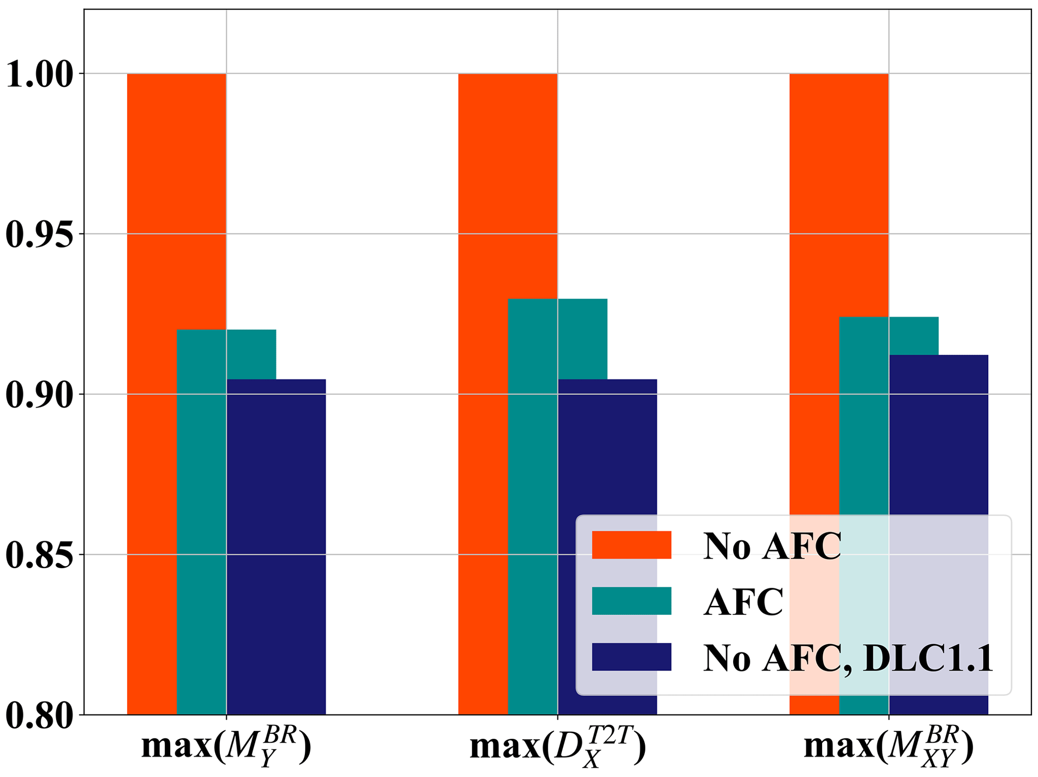
Figure 10 Normalized values of max($M_Y^{\mathrm{BR}}$), max($D_X^{\mathrm{T}\mathrm{2}\mathrm{T}}$) and max($M_{XY}^{\mathrm{BR}}$). Results are shown for all simulations without active flaps (No AFC), with active flaps (AFC) and for DLC 1.1 only.

It is also interesting to see what effect an active flap system has on the different load directions of max($M_{XY}^{\mathrm{BR}}$) around the blade root. Figure 11 shows the averaged value of max($M_{XY}^{\mathrm{BR}}$) for different load directions. We can see that the largest values of max($M_{XY}^{\mathrm{BR}}$) occur for angular bins between 70 and 100^∘. These angles are around the value of positive $M_Y^{\mathrm{BR}}$ (90^∘). Because we are only considering the DLC 1.1 and 1.3 groups, we will only have a good estimation for the extreme resulting bending moments due to the maximum thrust of the wind turbine, which happens to correspond to this region.

When we look at the effect of the active flap system, we can see that the reduction of max($M_{XY}^{\mathrm{BR}}$) occurs in this angular range. In the rest of the angular bins, the maximum resulting bending moments are practically identical. This can be understood if we recall that the controller input only included strain gauge information in the out-of-plane direction. Extreme resulting bending moments that arise from the combination of $M_Y^{\mathrm{BR}}$ and $M_X^{\mathrm{BR}}$ cannot be captured by the controller sensors. In addition, the flaps' control authority is mainly on the lift, so flap actuation will have little effect on the variation in $M_X^{\mathrm{BR}}$. Again, the reduction due to flap activity seen in Fig. 11 reduces the values of $M_{XY}^{\mathrm{BR}}$ to values close to the ones obtained from considering the loads from DLC 1.1 only.

5.5 Discussion

The results obtained in the previous section show that active TE flaps are able to reduce extreme loads and critical deflections of the blade substantially. Given the constraint that the control strategy should not interfere with the normal power production (DLC 1.1), a reduction of 7.6 % in max($M_{XY}^{\mathrm{BR}}$) is significant because it almost eliminates the increased extrema in DLC 1.3 due to the extreme turbulence (Fig. 10). These results are statistical and should be interpreted as an average performance of the flap system. To better understand the potentials and limitations of the proposed system, it is useful to look at some exemplary time series.

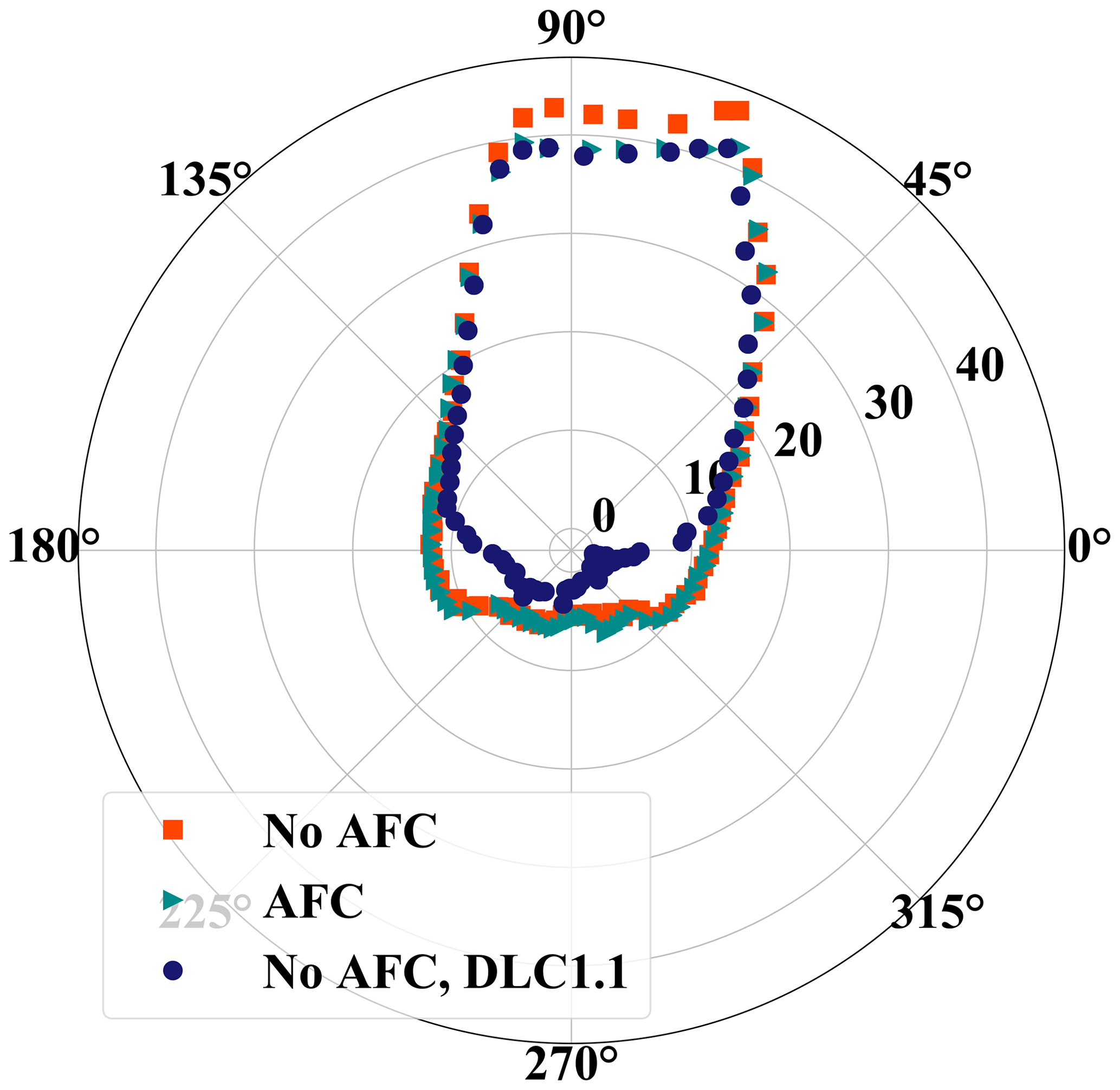
Figure 11 Averaged max($M_{XY}^{\mathrm{BR}}$) for different load directions. In this figure 0^∘ corresponds to positive $M_X^{\mathrm{BR}}$ and 90^∘ to positive $M_Y^{\mathrm{BR}}$. The radial coordinate is given in mega-newton-meters.

Figure 12 shows a selection of the time series for two simulations from the ${\stackrel{\mathrm{‾}}{V}}_{\mathrm{hub}}=\mathrm{11}$ m s⁻¹ wind speed bin, where several of the maxima occurred. Each column corresponds to one simulation. The first column shows a scenario where the average wind speed (not shown) is increasing and Ω is rising to values around rated rotor speed (Fig. 12d). The low value of β (Fig. 12c) leads to high values of rotor thrust and high values of $M_Y^{\mathrm{BR}}$ (Fig. 12a) and to the activation of the flaps (Fig. 12b). We can see that the flaps are being deployed even if the values of $M_Y^{\mathrm{BR}}$ do not reach an apparent peak. This is because Fig. 12a only shows the value of $M_Y^{\mathrm{BR}}$ for one blade, and all flaps are activated as soon as the deployment criteria are met by any blade. Let us now consider the situation around the simulation time of 520 s. Here the blade passes a local wind gust, and it significantly increases the value of $M_Y^{\mathrm{BR}}$ for the simulation without flaps. This also accelerates the rotor and activates the pitch system. This does not happen in the simulation with active flaps. Due to a previous activation of the flap system, the blade enters the wind gust with deployed flaps, thereby creating less lift and thus reducing the load peak by about 16 %. This is one example showing the large potential that active flap systems have in reducing the extreme loads of wind turbine blades.

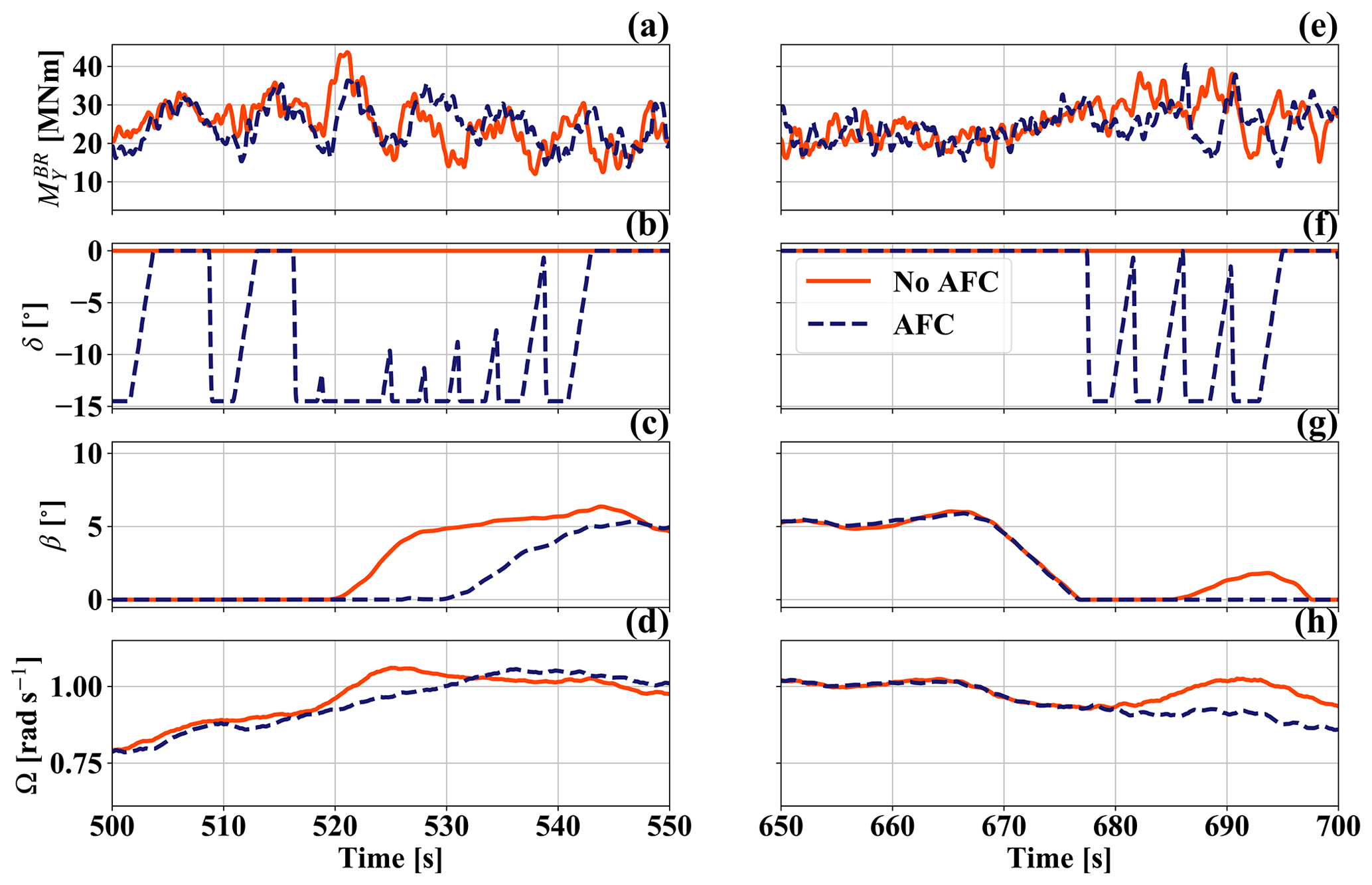
Figure 12 Selection of time series for two different simulations with ${\stackrel{\mathrm{‾}}{V}}_{\mathrm{hub}}=\mathrm{11}$ m s⁻¹. Panels (a–d) correspond to one simulation while panels (e–h) correspond to the second simulation.

The second column shows a situation where the controller does not perform as desired. At around 685 s of simulation time, there is a sudden peak in $M_Y^{\mathrm{BR}}$ for the simulations with active flaps (Fig. 12e). Just before that event the flaps had just arrived at their 0^∘ position, thus allowing the blade to generate normal lift (Fig. 12f). The flap controller reacts quickly, but the reaction is not quick enough to mitigate the high loading. Because we are trying to reduce the extreme loads, such events – although rare – are the ones that lead to the recorded maxima. In the case of this particular simulation, the extreme load reduction of the active flap system is only about 1.5 %. This example also illustrates well the necessity of having fast reactions from the flap system to sudden changes. This can only be obtained by including local sensorial information of the flap system – such as the flap hinge moment and acceleration signals – as part of the controller input.

One challenge in this particular study is that the difference in extrema between the DLC 1.1 and 1.3 groups is relatively small. Given the fact that the flap system needs a certain amount of time to have an effect on $M_Y^{\mathrm{BR}}$, we require the values of the different thresholds to be low. On the other hand they should not be too low in order to avoid influencing the normal power production of the turbine. The combination of these two requirements does not leave much room for threshold selection. Slightly changing the threshold values helped improve the performance of the flap system in certain scenarios but lowered the performance in others, thus giving similar results overall. If the difference in extreme conditions between the DLC 1.1 group and other DLC groups is higher (as was reported in Barlas et al., 2016b), then this issue becomes less critical.

Another observed issue with the proposed strategy is the unwanted mutual influence between the pitch and the flap controllers. We can see an example of this in Fig. 12c. The deployment of the flaps lowers the lift force but also the torque produced by the rotor and thus the rotor acceleration. This results in the pitch controller leaving the pitch angle longer at 0^∘ compared to a simulation without active flaps. While the overall effect on the rotor speed and hence generator power is small, the effects on $M_Y^{\mathrm{BR}}$ are more substantial. Lower values of β increase the values of α along the blade, leading to higher lift values and higher values of $M_Y^{\mathrm{BR}}$. It was observed in some simulations that there were values of max($M_Y^{\mathrm{BR}}$) with fully deployed flaps comparable to values of max($M_Y^{\mathrm{BR}}$) from the same simulations without active flaps. The difference lay in the respective values of β in each simulation. The influence of the flap controller led to lower values of β compared to the simulation without active flaps, indirectly reducing its effectiveness.

A possible solution would be to decrease the value of τ_dep or increase the flap rate when returning to the 0^∘ position, thus lowering the time that the flaps influence lift production. Because of the constraints in threshold selection mentioned before, having a flap deployment cycle that is too fast could lead to an unstable behavior where the flap system amplifies the blade oscillation. Another possible solution could be to adapt the controller so that each blade uses its flap system independently. While this strategy reduces the interference between the flap and the pitch controllers, it loses the information about the inflow conditions of the preceding blade. This leads to more false negative scenarios such as the one described in Fig. 12e–h, again lowering the effectiveness of the strategy.

All of the limitations discussed above arise mainly from the chosen controller strategy. While being simple, robust and able to reduce extreme loads and deflections significantly, the proposed architecture shows its limits when used in such a challenging scenario. Other controller strategy types, such as, e.g., model-based or adaptive-data-driven controllers that include combined pitch and flap action, are possible candidates that could exploit the full potential of active flaps while overcoming the observed limitations in this study.

6 Conclusions

In this paper we explored the potential of active trailing edge flaps to reduce extreme loads and critical deflections of the modified DTU 10 MW RWT blade with flaps. We considered the flap hinge moment as a robust and available sensor that can deliver valuable local information about the inflow and enable the flap system to have more time to react to sudden extreme conditions.

In order to use the flap hinge moment as an input sensor for a controller strategy, we adapted an existing unsteady hinge moment model for thin airfoils from the literature to use it in aero-servo-elastic simulations in the time domain. Based on this model, we developed an observer that estimates the effective local angle of attack and relative wind velocity of a blade section from local sensors. The latter include the flap hinge moment and an accelerometer mounted on the blade section.

We evaluated the performance of the observer in aeroelastic simulations with steady and turbulent wind conditions. For steady wind conditions, the error between the estimated and real values of the mean V_rel was below 0.4 % for all wind speeds between 4 and 24 m s⁻¹. The error between the estimated and real value of the mean α lay below 0.2^∘. We also tested the observer in more challenging turbulent wind speed conditions. Although our observer was lacking information about the incoming turbulent wind, it was able to estimate the low-frequency content of V_rel and α fairly well. An exception was seen to be the local turbulent gust slicing of the blade for higher wind speeds. This leads to increased 1P variations in V_rel not captured by the observer.

This observer was included in a simple flap controller strategy to mitigate extreme blade loads and critical blade deflections. It is based on a series of on-off criteria applied to several input sensors. The sensors included integrated load values – such as $M_Y^{\mathrm{BR}}$ – and local information of the individual blade sections – such as M_Hin, $\dot{x}$, $\widehat{\mathit{\alpha }}$ and ${\widehat{V}}_{\mathrm{rel}}$.

We tested the performance of this strategy in aero-servo-elastic load calculations according to the DLC 1.3 group from the IEC standard. This group features the extreme turbulent wind model and is responsible for the maxima of $M_Y^{\mathrm{BR}}$ and $D_X^{\mathrm{T}\mathrm{2}\mathrm{T}}$ of our considered blade. The simulations were performed using the LLFVW aerodynamic model, which has been shown to calculate aerodynamic loads more accurately than the conventional BEM aerodynamic models. The proposed flap controller was able to reduce the maxima of $M_Y^{\mathrm{BR}}$ and $M_{XY}^{\mathrm{BR}}$ by 8 % and 7.6 %, respectively. The controller was also able to reduce the critical blade deflection – i.e., the blade tip deflection in front of the tower – by 7.1 %. Looking at the maxima of $M_{XY}^{\mathrm{BR}}$ for different load directions, we found that the flap controller was able to reduce max($M_{XY}^{\mathrm{BR}}$) for angular bins between 70 and 100^∘, bringing them down to values that are comparable to the maxima from normal power production load cases. These directions correspond to directions around positive $M_Y^{\mathrm{BR}}$, where the flap control authority is also highest for a blade with β=0^∘.

A more detailed look revealed that active flap systems in general have the potential to reduce the extreme loads even further. Yet a combination of challenging conditions – e.g., constraints in the parameter selection space in order to reduce extreme loads without interfering with normal power production – and a simple controller strategy were found to be the main limitations of the proposed system.

The results of this paper show that active TE flaps have a large potential to reduce design-driving extreme loads and critical deflections of wind turbine blades. They can therefore help create more competitive turbine designs that will reduce the cost of energy even further. A critical aspect was seen to be the reaction time of the active flap system, which can be greatly improved if local sensors – such as the flap hinge moment – are used as input for the control strategy. More work needs to be done in order to gain further insight into this topic and better quantify the aforementioned potential of flaps.

The model used for the hinge moment calculation could be improved to increase its accuracy. Further refinements could include a more detailed state-space representation of the aerodynamic loads, include other inertial loads such as centrifugal and gyroscopic loads, and also include friction.

In this study we used identical systems to model the flap hinge and as input for our observer. This is certainly unrealistic, and a robustness study should be done to quantify how model uncertainty and measurement noise affect the observer performance. This is especially of relevance due to the lower sensitivity of the hinge moment coefficient to changes in the angle of attack. A proof of stability for the LPV observer is also needed to guarantee that the observer will be stable at all times.

The model and observer should also be tested experimentally. On the one hand, the proposed model could be compared to experimental data obtained from a 2D airfoil with an active flap for different reduced frequencies. Alternatively or complementarily, a system identification could be performed using experimental data to create an unsteady hinge moment model from the data to be used in the observer. The observer and model could also be tested and analyzed experimentally using an experimental wind turbine in a wind tunnel.

Regarding the controller strategy, a better quantification of its performance can be obtained by including more DLC groups that include the load extrema in all directions. Also, the evaluation of the strategy should be extended to include more load sensors, such as hub and tower bending moments. In addition, other control strategies should be considered as possible candidates for extreme load and deflection control. In particular, model-based or adaptive-data-driven controllers that are able to control both the pitch and flap actuators are promising candidates to increase the ability of active flaps to reduce design-driving loads.

Appendix A: Entries of the hinge model and observer state-space matrices

This appendix contains the explicit entries of the matrices used for the hinge model and the hinge model observer. The entries for the feedthrough matrix of the hinge model D_Hin are as follows.

$$\begin{array}{}\text{(A1)}& {\displaystyle }& {\displaystyle }{D}_{\mathit{\alpha }}={\displaystyle \frac{{\mathit{ϵ}}_{\mathit{\alpha }}\cdot F_{\mathrm{12}}}{\mathrm{4}}}\text{(A2)}& {\displaystyle }& {\displaystyle }{D}_{\dot{\mathit{\alpha }}}={\displaystyle \frac{{\mathit{ϵ}}_{\mathit{\alpha }}\cdot F_{\mathrm{12}}\cdot b\cdot (\mathrm{1}/\mathrm{2}-a)}{\mathrm{4}{V}_{\mathrm{rel}}}}-{\displaystyle \frac{b\cdot \left(-\mathrm{2}{F}_{\mathrm{9}}-F_{\mathrm{1}}+F_{\mathrm{4}}\cdot (a-\mathrm{1}/\mathrm{2})\right)}{\mathrm{2}{V}_{\mathrm{rel}}}}\text{(A3)}& {\displaystyle }& {\displaystyle }{D}_{\ddot{\mathit{\alpha }}}={\displaystyle \frac{-F_{\mathrm{13}}\cdot b^{\mathrm{2}}}{V_{\mathrm{rel}}^{\mathrm{2}}}}\text{(A4)}& {\displaystyle }& {\displaystyle }{D}_{\mathit{\delta }}={\displaystyle \frac{{\mathit{ϵ}}_{\mathit{\delta }}\cdot F_{\mathrm{12}}\cdot F_{\mathrm{10}}}{\mathrm{4}\mathit{\pi }}}-{\displaystyle \frac{F_{\mathrm{5}}-F_{\mathrm{4}}\cdot F_{\mathrm{10}}}{\mathrm{2}\mathit{\pi }}}\text{(A5)}& {\displaystyle }& {\displaystyle }{D}_{\dot{\mathit{\delta }}}={\displaystyle \frac{{\mathit{ϵ}}_{\mathit{\delta }}\cdot F_{\mathrm{12}}\cdot b\cdot F_{\mathrm{11}}}{\mathrm{8}\mathit{\pi }\cdot V_{\mathrm{rel}}}}+{\displaystyle \frac{b\cdot F_{\mathrm{4}}\cdot F_{\mathrm{11}}}{\mathrm{4}\mathit{\pi }\cdot V_{\mathrm{rel}}}}\text{(A6)}& {\displaystyle }& {\displaystyle }{D}_{\ddot{\mathit{\delta }}}={\displaystyle \frac{F_{\mathrm{3}}\cdot b^{\mathrm{2}}}{\mathrm{2}\mathit{\pi }\cdot V_{\mathrm{rel}}^{\mathrm{2}}}}\end{array}$$

$$\begin{array}{}\text{(A7)}& {\displaystyle }& {\displaystyle }{D}_{\dot{h}}={\displaystyle \frac{{\mathit{ϵ}}_{\mathit{\alpha }}\cdot F_{\mathrm{12}}}{\mathrm{4}{V}_{\mathrm{rel}}}}\text{(A8)}& {\displaystyle }& {\displaystyle }{D}_{\ddot{h}}={\displaystyle \frac{F_{\mathrm{1}}\cdot b}{\mathrm{2}{V}_{\mathrm{rel}}^{\mathrm{2}}}}\end{array}$$

The geometric constants F_i depend on the flap size relative to the airfoil chord and are given in Hariharan and Leishman (1995).

For the hinge observer model, the explicit entries of ${\mathbf{B}}_{\mathrm{Hin}}^{\mathit{\alpha }}$ and ${\mathbf{B}}_{\mathrm{Hin}}^{\mathrm{Res}}$ are

$$\begin{array}{}\text{(A9)}& {\displaystyle }& {\displaystyle }{\mathbf{B}}_{\mathrm{Hin}}^{\mathit{\alpha }}=\left[\begin{array}{ccc}\mathrm{0}& \mathrm{0}& \mathrm{0}\\ \mathrm{1}& b\cdot \frac{(\mathrm{1}/\mathrm{2}-a)}{V_{\mathrm{rel}}}& \mathrm{0}\\ \mathrm{0}& \mathrm{0}& \mathrm{0}\\ \mathrm{0}& \mathrm{0}& \mathrm{0}\end{array}\right],\text{(A10)}& {\displaystyle }& {\displaystyle }{\mathbf{B}}_{\mathrm{Hin}}^{\mathrm{Res}}=\left[\begin{array}{ccccc}\mathrm{0}& \mathrm{0}& \mathrm{0}& \mathrm{0}& \mathrm{0}\\ \mathrm{0}& \mathrm{0}& \mathrm{0}& \frac{\mathrm{1}}{V_{\mathrm{rel}}}& \mathrm{0}\\ \mathrm{0}& \mathrm{0}& \mathrm{0}& \mathrm{0}& \mathrm{0}\\ \frac{F_{\mathrm{10}}}{\mathit{\pi }}& \frac{b\cdot F_{\mathrm{11}}}{\mathrm{2}\mathit{\pi }\cdot V_{\mathrm{rel}}}& \mathrm{0}& \mathrm{0}& \mathrm{0}\end{array}\right].\end{array}$$

Appendix B: List of symbols, subscripts and superscripts

This section contains the list of symbols (Tables B1 and B2) as well as the list of sub- and superscripts (Table B3) .

Table B1 List of Latin symbols used in this paper.

Table B2 List of Greek symbols used in this paper.

Table B3 List of sub- and superscripts.