A method for preliminary rotor design – Part 1: Radially Independent Actuator Disc model

We present an analytical model for assessing the aerodynamic performance of a wind turbine rotor through a different parametrization of the classical blade element momentum (BEM) model. The model is named the Radially Independent Actuator Disc (RIAD) model, and it establishes an analytical relationship between the local thrust loading and the local power, known as the local-thrust coefficient and the local-power coefficient respectively. The model has a direct physical interpretation, showing the contribution for each of the three losses: wake rotation loss, tip loss and viscous loss. The gradient for RIAD is found through the use of the complex step method, and power optimization is used to show how easily the method can be used for rotor optimization. The main benefit of RIAD is the ease with which it can be applied for rotor optimization and especially load constraint power optimization as described in Loenbaek et al. (2021). The relationship between the RIAD input and the rotor chord and twist is established, and it is validated against a BEM solver.

1 Introduction

Wind turbine rotors are with their increasing size subject to continuous optimization, with the overall objective of reducing the cost of energy. Such optimizations are very complex because both the aerodynamic and the structural performance need to be included in the optimization setup. Combining both aerodynamics and structural performance has shown very promising trends indicating that a further cost reduction is possible; see, e.g., Perez-Moreno et al. (2016), Zahle et al. (2015) and Bottasso et al. (2012). However, these optimization studies build on existing aerodynamic and aeroelastic tools, include numerous design variables and constraints, and can be very complex. Thus, it is challenging to make a very general optimization study to map the design space. That is the reason for investigating alternative methods and models to ease the exploration of optimal rotor designs.

The development of aerodynamic models for wind turbines is closely linked to that of propellers and helicopters. The first theoretical model for predicting the aerodynamic performance of a rotor was the so-called 1D momentum theory developed by Betz (Betz, 1926) and Joukowsky, which resulted in the famous maximum power extraction limit of 59.3 % known as the Betz–Joukowsky limit or often just as the Betz limit (Okulov and van Kuik, 2012). The model assumed constant loading along the rotor radius in the flow direction.

Later Glauert developed the blade element momentum (BEM) theory (Durand and Glauert, 1935; Sørensen, 2016), which is an extension where momentum theory is used for radially independent stream tubes. It also included correction models for tip loss and highly loaded rotors. The model has since then been extended with multiple correction models to account for yaw misalignment, shear profiles, turbulent inflow, etc.

In this paper, we present an aerodynamic rotor performance model which we refer to as the Radially Independent Actuator Disc (RIAD) model. It establishes a direct analytical relationship between the local thrust loading and the local power, which is a useful simplification for rotor optimization. The model is equivalent to BEM but reduces the rotor design space to only two independent variables at each radial station, i.e., the local-thrust coefficient (C_LT) and the glide ratio ($C_{\mathrm{l}}/C_{\mathrm{d}}$) as well as the global tip speed ratio (λ). The equivalent input for a BEM at each radial station is the design lift coefficient (C_l), the design drag coefficient (C_d) and the rotor solidity (σ) with the same global parameter. Most BEM formulations do not compute the local power directly, which is often an important optimization objective. At the same time, rotor optimization constraints are often formulated in terms of loading. Both the objective and constraints are outputs from the BEM, and their equations are usually fairly convoluted. Using RIAD, the local thrust loading (C_LT) is the independent design parameter, and the local power is computed explicitly through a single equation. It makes it easy to recast the optimization problem, which generally requires a robust optimization algorithm, into a straightforward root-finding problem, which makes the optimization faster and more robust.

The paper starts by presenting the derivation of the RIAD model, which then leads into computing the gradients for RIAD. These gradients are used for power optimization, leading to a simple optimization method. In the end, the relationship between RIAD inputs and blade chord and twist is then established, and RIAD is validated against a BEM solver. This is Part 1 of a two-part paper. Part 1 describes an aerodynamic model for a wind turbine rotor and the use of the model for power optimization. Part 2 is described in Loenbaek et al. (2021), where the model is applied for load-constrained power optimization.

2 The RIAD model

In the following the Radially Independent Actuator Disc (RIAD) model is presented, which starts by establishing the relationship between global and local parameters for a wind turbine rotor as well as introducing normalization. The relationship between the local forces is then established, leading to an implicit equation for the local power. A set of approximate closure equations is then used to establish an explicit equation. The physical interpretation of the different factors and terms is then presented, and at the end some details regarding the tip loss factor and the exclusion of drag from the induced velocity are discussed.

2.1 Relationship between global and local coefficients

Starting with the fundamental theorem of calculus the following equation can be created for the global values for thrust (T) and power (P):

$$\begin{array}{}\text{(1)}& T=\underset{\mathrm{0}}{\overset{R}{\int }}{\displaystyle \frac{\partial T}{\partial r}}\mathrm{d}r,\end{array}$$

$$\begin{array}{}\text{(2)}& P=\underset{\mathrm{0}}{\overset{R}{\int }}{\displaystyle \frac{\partial P}{\partial r}}\mathrm{d}r,\end{array}$$

where $\frac{\partial T}{\partial r}$ is the thrust loading density and $\frac{\partial P}{\partial r}$ is the power density.

The classical non-dimensional relations for thrust (C_T) and power (C_P) as well as the local equivalent which is introduced as the local-thrust coefficient (C_LT) and local-power coefficient (C_LP) are introduced as follows:

$$\begin{array}{}\text{(3)}& {\displaystyle }& {\displaystyle }T={\displaystyle \frac{\mathrm{1}}{\mathrm{2}}}{\mathit{\rho }}_{\mathrm{0}}{V}^{\mathrm{2}}\mathit{\pi }{R}^{\mathrm{2}}{C}_{\mathrm{T}},\text{(4)}& {\displaystyle }& {\displaystyle }P={\displaystyle \frac{\mathrm{1}}{\mathrm{2}}}{\mathit{\rho }}_{\mathrm{0}}{V}^{\mathrm{3}}\mathit{\pi }{R}^{\mathrm{2}}{C}_{\mathrm{P}},\text{(5)}& {\displaystyle }& {\displaystyle \frac{\partial T}{\partial r}}={\displaystyle \frac{\mathrm{1}}{\mathrm{2}}}\mathit{\rho }\mathrm{2}\mathit{\pi }r{V}^{\mathrm{2}}{C}_{\mathrm{LT}},\text{(6)}& {\displaystyle }& {\displaystyle \frac{\partial P}{\partial r}}={\displaystyle \frac{\mathrm{1}}{\mathrm{2}}}\mathit{\rho }\mathrm{2}\mathit{\pi }r{V}^{\mathrm{3}}{C}_{\mathrm{LP}}.\end{array}$$

Combining the equations, the following equations can be found for C_T and C_P:

$$\begin{array}{}\text{(7)}& {\displaystyle }& {\displaystyle }{C}_{\mathrm{T}}=\mathrm{2}\underset{\mathrm{0}}{\overset{\mathrm{1}}{\int }}{C}_{\mathrm{LT}}\stackrel{\mathrm{̃}}{r}\mathrm{d}\stackrel{\mathrm{̃}}{r},\text{(8)}& {\displaystyle }& {\displaystyle }{C}_{\mathrm{P}}=\mathrm{2}\underset{\mathrm{0}}{\overset{\mathrm{1}}{\int }}{C}_{\mathrm{LP}}\stackrel{\mathrm{̃}}{r}\mathrm{d}\stackrel{\mathrm{̃}}{r},\end{array}$$

where $\stackrel{\mathrm{̃}}{r}$ is the normalized radius ($\stackrel{\mathrm{̃}}{r}=r/R$). A diagram of the relationship between the local and global coefficients can be seen in Fig. 1.

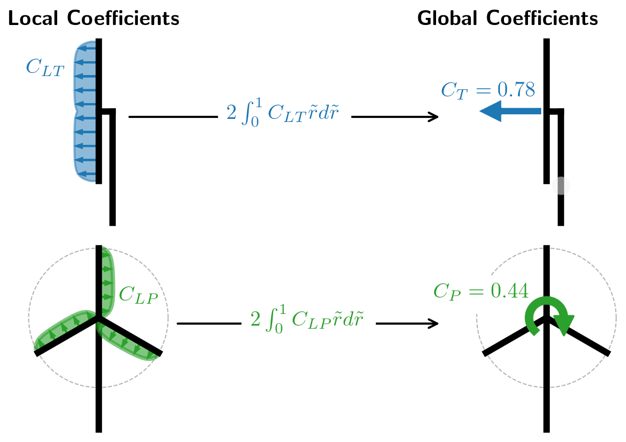
Figure 1 Diagram of the relationship between local coefficients (C_LT, C_LP) and global coefficients (C_T, C_P).

2.2 Relationship between local coefficients

To establish a relationship between the local coefficients C_LT and C_LP, the forces are assumed to be aerodynamic forces where the lift force is orthogonal to the local flow and where there is loss from viscous drag in the local flow direction. The force is assumed to originate from rotating wind turbine blades with rotational speed ω. The tangential force density is then given as $\frac{\mathrm{1}}{\mathit{\omega }r}\frac{\partial P}{\partial r}$. Introducing the local lift density $\frac{\partial L}{\partial r}$ and drag density $\frac{\partial D}{\partial r}$ as well as the local flow angle ϕ, the following equations can be created:

$$\begin{array}{}\text{(9)}& {\displaystyle }& {\displaystyle \frac{\partial T}{\partial r}}={\displaystyle \frac{\partial L}{\partial r}}\cos \mathit{\varphi },\text{(10)}& {\displaystyle }& {\displaystyle \frac{\mathrm{1}}{\mathit{\omega }r}}{\displaystyle \frac{\partial P}{\partial r}}={\displaystyle \frac{\partial L}{\partial r}}\sin \mathit{\varphi }-{\displaystyle \frac{\partial D}{\partial r}}\cos \mathit{\varphi },\end{array}$$

where $\partial D/\partial r=\mathrm{0}$ in Eq. (9) to exclude drag from induction. Using the common normalization of $\partial L/\partial r$ and $\partial D/\partial r$,

$$\begin{array}{}\text{(11)}& {\displaystyle }& {\displaystyle \frac{\partial L}{\partial r}}={\displaystyle \frac{\mathrm{1}}{\mathrm{2}}}\mathit{\rho }Bc{V}_{\mathrm{rel}}^{\mathrm{2}}{C}_{\mathrm{l}},\text{(12)}& {\displaystyle }& {\displaystyle \frac{\partial D}{\partial r}}={\displaystyle \frac{\mathrm{1}}{\mathrm{2}}}\mathit{\rho }Bc{V}_{\mathrm{rel}}^{\mathrm{2}}{C}_{\mathrm{d}},\end{array}$$

together with Eqs. (5) and (6), the following equations can be found:

$$\begin{array}{}\text{(13)}& {\displaystyle }& {\displaystyle }{C}_{\mathrm{LT}}=\mathit{\sigma }{\stackrel{\mathrm{̃}}{V}}_{\mathrm{rel}}^{\mathrm{2}}{C}_{\mathrm{l}}\cos \mathit{\varphi },\text{(14)}& {\displaystyle }& {\displaystyle \frac{C_{\mathrm{LP}}}{\mathit{\lambda }\stackrel{\mathrm{̃}}{r}}}=\mathit{\sigma }{\stackrel{\mathrm{̃}}{V}}_{\mathrm{rel}}^{\mathrm{2}}{C}_{\mathrm{l}}\sin \mathit{\varphi }-\mathit{\sigma }{\stackrel{\mathrm{̃}}{V}}_{\mathrm{rel}}^{\mathrm{2}}{C}_{\mathrm{d}}\cos \mathit{\varphi },\end{array}$$

where σ is the rotor solidity ($\mathit{\sigma }=Bc/\mathrm{2}\mathit{\pi }r$) and ${\stackrel{\mathrm{̃}}{V}}_{\mathrm{rel}}$ the normalized relative velocity. A diagram of the airflow and forces can be seen in Fig. 2.

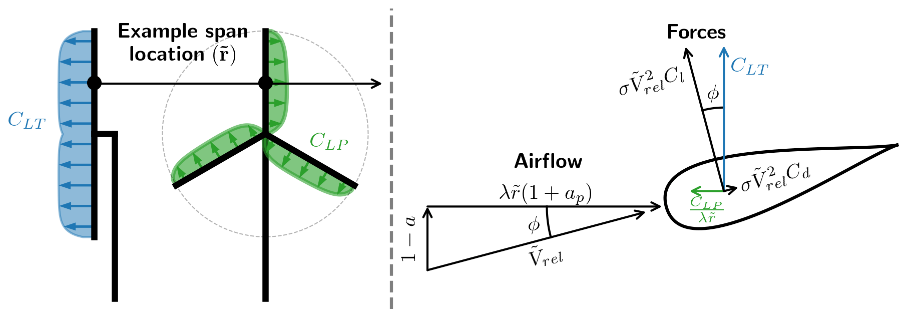
Figure 2 Diagram of the relationship between the airflow and the forces at each span location.

Combining Eqs. (13) and (14) an equation for C_LP can be found as

$$\begin{array}{}\text{(15)}& C_{\mathrm{LP}}\left(C_{\mathrm{LT}},\stackrel{\mathrm{̃}}{r},\mathit{\lambda },{\displaystyle \frac{C_{\mathrm{d}}}{C_{\mathrm{l}}}},\mathit{\varphi }\right)=\mathit{\lambda }\stackrel{\mathrm{̃}}{r}{C}_{\mathrm{LT}}\tan \mathit{\varphi }-\mathit{\lambda }\stackrel{\mathrm{̃}}{r}{\displaystyle \frac{C_{\mathrm{d}}}{C_{\mathrm{l}}}}{C}_{\mathrm{LT}}.\end{array}$$

This is a general equation for the relationship between the C_LT and C_LP, but it is implicit since tan ϕ depends on C_LT.

2.3 Explicit equation for C_LP (closure relation between C_LT and tan ϕ)

The local flow angle ϕ is given from the induced velocities (Sørensen, 2016, p. 101, Eq. 7.3) as

$$\begin{array}{}\text{(16)}& \tan \mathit{\varphi }={\displaystyle \frac{\mathrm{1}-a}{\mathit{\lambda }\stackrel{\mathrm{̃}}{r}\left(\mathrm{1}+a_p\right)}},\end{array}$$

where a is the axial induction factor and a_p is the tangential induction factor.

Equation (16) introduces two new variables (a, a_p). In order to make an explicit equation for tan ϕ as a function of C_LT two equations relating C_LT to a and a_p respectively are needed. These are the closure equations.

There does not exist a general set of model closure equations, but different approximate closures have been proposed. The most widely used set is referred to as the Glauert closure, which is an implicit assumption made for most BEMs. The closures are given as

$$\begin{array}{}\text{(17)}& {\displaystyle }{C}_{\mathrm{LT}}=\mathrm{4}a(\mathrm{1}-a)F(\mathrm{Ning},\mathrm{2014},\mathrm{p}.\mathrm{4}\mathrm{Eq}.\mathrm{2}),\text{(18)}& {\displaystyle }\begin{array}{rl}a(\mathrm{1}-a)={\mathit{\lambda }}^{\mathrm{2}}{\stackrel{\mathrm{̃}}{r}}^{\mathrm{2}}{a}_p\left(\mathrm{1}+a_p\right)& (\mathrm{S}\mathrm{ø}\mathrm{rensen},\mathrm{2016},\mathrm{p}.\mathrm{50}\\ & \mathrm{Eq}.\mathrm{4.36}),\end{array}\end{array}$$

where F is the tip loss factor, which is further described in Sect. 2.5. For now $F\in ]\mathrm{0},\mathrm{1}]$ with F→0 as $\stackrel{\mathrm{̃}}{r}\to \mathrm{1}$. Combining Eqs. (17) and (18) with Eq. (16) an explicit equation for tan ϕ in terms of C_LT can be found. This leads to an explicit equation for C_LP:

$$\begin{array}{}\text{(19)}& \begin{array}{rl}{C}_{\mathrm{LP}}\left(C_{\mathrm{LT}},\stackrel{\mathrm{̃}}{r},\mathit{\lambda },{\displaystyle \frac{C_{\mathrm{d}}}{C_{\mathrm{l}}}}\right)& =\underset{\mathrm{1}\mathrm{D}\mathrm{power}}{\underbrace{{\displaystyle \frac{\mathrm{1}}{\mathrm{2}}}\left(\mathrm{1}+\sqrt{\mathrm{1}-{\displaystyle \frac{C_{\mathrm{LT}}}{F}}}\right)C_{\mathrm{LT}}}}\\ & \cdot \underset{\mathrm{wake}\mathrm{rotation}\mathrm{loss}}{\underbrace{{\displaystyle \frac{\mathrm{2}\mathit{\lambda }\stackrel{\mathrm{̃}}{r}}{\mathit{\lambda }\stackrel{\mathrm{̃}}{r}+\sqrt{{\mathit{\lambda }}^{\mathrm{2}}{\stackrel{\mathrm{̃}}{r}}^{\mathrm{2}}+\frac{C_{\mathrm{LT}}}{F}}}}}}-\underset{\mathrm{viscous}\mathrm{loss}}{\underbrace{\mathit{\lambda }\stackrel{\mathrm{̃}}{r}{\displaystyle \frac{C_{\mathrm{d}}}{C_{\mathrm{l}}}}{C}_{\mathrm{LT}}}}.\end{array}\end{array}$$

Equation (19) is the main result of this section. It states an explicit relationship between the local power and the local loading.

Figure 3 Diagram showing a graphical representation of the losses and the mathematical origin. The input is for spanwise constant local thrust and glide ratio.

2.4 Physical interpretation and input sensitivity

Equation (19) has a straightforward physical interpretation which is also highlighted through under-bracing of factors and terms, with an additional loss coming from the tip loss factor (F). A diagram showing the impact of different losses for a specific input can be seen in Fig. 3.

The 1D power is the classical 1D momentum theory result by Betz and Joukowsky (Okulov and van Kuik, 2012), but here it is applied for radially independent stream tubes, noting the following relation:

$${\displaystyle \frac{\mathrm{1}}{\mathrm{2}}}\left(\mathrm{1}+\sqrt{\mathrm{1}-C_{\mathrm{LT}}}\right)C_{\mathrm{LT}}=\mathrm{4}a(\mathrm{1}-a{)}^{\mathrm{2}}.$$

The wake rotation loss is the power loss that originates from the conservation of angular momentum. When extracting power from the rotational motion, the force that is rotating the blades leads to an opposing and equal magnitude force on the fluid, resulting in the fluid rotating in the wake of the turbine. Since there needs to be conservation of power, the potential power that can be extracted is lowered, leading to wake rotation loss. From Fig. 3 the wake rotation loss is seen to affect the root region of turbine. This is further investigated in Fig. 4, where the wake rotation loss factor is plotted as a function of the local tip speed ratio ($\mathit{\lambda }\stackrel{\mathrm{̃}}{r}$) for different values of the local loading (C_LT).

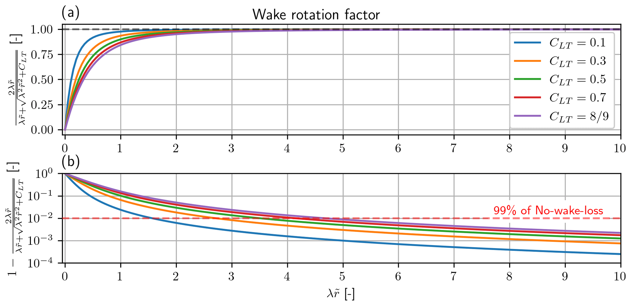
Figure 4 Significance of wake rotation loss. (a) Wake rotation factor vs. local tip speed ratio ($\mathit{\lambda }\stackrel{\mathrm{̃}}{r}$). The black dashed line is the limit at $\mathrm{1}/\mathrm{2}$. (b) Difference between the wake rotation factor and the limit at $\mathrm{1}/\mathrm{2}$ vs. local tip speed ratio ($\mathit{\lambda }\stackrel{\mathrm{̃}}{r}$). Note that the y axis is log scale. The red dashed line is at 99 % of the limit. Note that the solid lines are for different values of C_LT. Higher C_LT leads to higher wake rotation loss.

The effect of changing the local loading is seen to have a limited effect. From Fig. 4b the wake rotation loss is seen to be insignificant for $\mathit{\lambda }\stackrel{\mathrm{̃}}{r}>\mathrm{5}$, which is approximately from the mid-span and outwards for a modern utility scale turbine with λ≈7–10. From the example in Fig. 3 the wake rotation loss is seen to have the smallest impact on the global power with $\mathrm{\Delta }{C}_{\mathrm{P}}=-\mathrm{0.01}$.

The tip loss is the power loss associated with the rotor having a finite number of blades and not acting as an actuator disc with an infinite number of blades. This effect is captured in the tip loss factor (F), which is further described in Sect. 2.5. The tip loss model that is used in this paper captures the impact on the induced velocities in the rotor plane, with the additionally induced velocities coming from the vorticity released at the tip of the blade. The most important parameter for tip loss is the tip speed ratio (λ), with the tip loss getting smaller with increasing tip speed ratio. From Fig. 3 the tip loss is seen to affect the power at the tip as one might expect (hub or root loss was not included but easily could have been).

The viscous loss is simply the loss associated with the viscous drag from the airfoil profile. The viscous loss is found to be linear in inverse glide ratio ($C_{\mathrm{d}}/C_{\mathrm{l}}$), loading (C_LT) and local tip speed ratio ($\mathit{\lambda }\stackrel{\mathrm{̃}}{r}$), with a larger value for each of them leading to a larger loss. In contrast to both wake rotation loss and tip loss, a larger tip speed ratio is found to result in larger losses. As a consequence, there will exist an optimal tip speed ratio since either extreme (λ→0, λ→∞) will lead to 0 or negative power. This is further discussed in Sect. 3.3. From Fig. 3 the loss is seen to increase towards the tip since the local tip speed ratio ($\mathit{\lambda }\stackrel{\mathrm{̃}}{r}$) is increasing. Viscous loss is seen to be the most significant loss of the three, although it should be noted that a glide ratio of $\frac{C_{\mathrm{l}}}{C_{\mathrm{d}}}=\mathrm{40}$ is a fairly low value for a realistic modern rotor design and is here chosen to make the loss easily visible for the figure.

2.5 Tip loss factor

The tip loss factor is commonly implemented for BEMs, and although some different tip correction has been proposed, the tip loss model by Glauert is a common one to use, and it is also the one used here. It is given as

$$\begin{array}{}\text{(20)}& \begin{array}{rl}F(\mathit{\varphi },\stackrel{\mathrm{̃}}{r},\mathit{\lambda })=& {\displaystyle \frac{\mathrm{2}}{\mathit{\pi }}}{\cos }^{-\mathrm{1}}\exp \left(-{\displaystyle \frac{B(\mathrm{1}/\stackrel{\mathrm{̃}}{r}-\mathrm{1})}{\mathrm{2}\sin \mathit{\varphi }}}\right)\\ & (\mathrm{S}\mathrm{ø}\mathrm{rensen},\mathrm{2016},\mathrm{p}.\mathrm{132}\mathrm{Eq}.\mathrm{8.29}),\end{array}\end{array}$$

where B is the number of blades (which for simplicity is set to three throughout the paper). The Glauert tip loss model leads to a recursive problem due to the mutual dependence between C_LT, sin ϕ and F. It is not possible to find an explicit equation for F in terms of C_LT, but it is possible to find a iterative scheme that can solve for F. The iterative scheme is given as

$$\begin{array}{}\text{(21)}& {\displaystyle }\begin{array}{rl}\sin {\mathit{\varphi }}_i& \left(C_{\mathrm{LT}},\stackrel{\mathrm{̃}}{r},\mathit{\lambda },F_i\right)=\\ & {\displaystyle \frac{\mathrm{1}+\sqrt{\mathrm{1}-\frac{C_{\mathrm{LT}}}{F_i}}}{\sqrt{{\left(\mathrm{1}+\sqrt{\mathrm{1}-\frac{C_{\mathrm{LT}}}{F_i}}\right)}^{\mathrm{2}}+\left(\mathit{\lambda }\stackrel{\mathrm{̃}}{r}+\sqrt{{\mathit{\lambda }}^{\mathrm{2}}{\stackrel{\mathrm{̃}}{r}}^{\mathrm{2}}+\frac{C_{\mathrm{LT}}}{F_i}}\right)\mathrm{2}}}},\end{array}\text{(22)}& {\displaystyle }{F}_{i+\mathrm{1}}\left(C_{\mathrm{LT}},\stackrel{\mathrm{̃}}{r},\mathit{\lambda },\sin {\mathit{\varphi }}_i\right)={\displaystyle \frac{\mathrm{2}}{\mathit{\pi }}}{\cos }^{-\mathrm{1}}\exp \left(-{\displaystyle \frac{B(\mathrm{1}/\stackrel{\mathrm{̃}}{r}-\mathrm{1})}{\mathrm{2}\sin {\mathit{\varphi }}_i}}\right),\end{array}$$

where an acceptable tolerance for F is reached with at most 30 iterations ($|F_{i+\mathrm{1}}-F_i|<{\mathrm{10}}^{-\mathrm{9}}$) where a good initial guess for F would be 1.

The Glauert tip loss model breaks the explicit relationship between C_LT and C_LP in Eq. (19), since F needs to be solved through iterations. An explicit relationship could be obtained by using the Prandtl tip loss model instead, which is given as

$$\begin{array}{}\text{(23)}& \begin{array}{rl}{F}_{\mathrm{Prandtl}}(\stackrel{\mathrm{̃}}{r},\mathit{\lambda })=& {\displaystyle \frac{\mathrm{2}}{\mathit{\pi }}}{\cos }^{-\mathrm{1}}\exp \left(-{\displaystyle \frac{B}{\mathrm{2}}}\sqrt{\mathrm{1}+{\mathit{\lambda }}^{\mathrm{2}}}\left(\mathrm{1}-\stackrel{\mathrm{̃}}{r}\right)\right)\\ & (\mathrm{S}\mathrm{ø}\mathrm{rensen},\mathrm{2016},\mathrm{p}.\mathrm{131},\mathrm{Eq}.\mathrm{8.26}),\end{array}\end{array}$$

which does not depend on C_LT. Using Prandtl's tip loss model, the effect on the tip loss is found to be larger compared to Glauert's tip loss model, but investigating it further here is outside the scope of this paper.

Although the Prandtl tip loss model is much simpler and easier to implement, the Glauert model is used throughout this paper as it is the one used for the BEM validation later in Sect. 4.2.

2.6 Blade loading without drag in induction

Whether or not to include drag when computing the thrust loading (including drag in Eq. 13) is still a standing question for the derivation of BEM, and excluding drag in the derivation here should not be seen as an argument in favor of this approach but merely as a consequence that makes the mathematical derivation simpler as well as the resulting equation for local power (Eq. 19). If drag should be included for the computation of the induced velocities, it should be noted that it is not just a matter of including drag in Eq. (13), as the closure equation in Eq. (18) also needs an additional $\mathit{\lambda }\stackrel{\mathrm{̃}}{r}\frac{C_{\mathrm{d}}}{C_{\mathrm{l}}}(a+a_p)$ to be added on the right-hand side if it should be consistent with the BEM described in Ning (2014).

As a consequence of excluding drag from Eq. (13), there arises a difference between the forces seen from the blade and the forces seen by the air, where Eq. (13) is the thrust force as seen by the air and where Eq. (14) is the tangential force seen by the blade. Often in optimization it is the thrust load at the blade that is of interest, and Eq. (24) shows the relationship between the two local thrust loadings:

$$\begin{array}{}\text{(24)}& \begin{array}{rl}{C}_{\mathrm{LT},\mathrm{blade}}& \left(C_{\mathrm{LT}},\stackrel{\mathrm{̃}}{r},\mathit{\lambda },{\displaystyle \frac{C_{\mathrm{d}}}{C_{\mathrm{l}}}}\right)\\ & =C_{\mathrm{LT}}\left(\mathrm{1}+{\displaystyle \frac{C_{\mathrm{d}}}{C_{\mathrm{l}}}}{\displaystyle \frac{\mathrm{1}+\sqrt{\mathrm{1}-\frac{C_{\mathrm{LT}}}{F}}}{\mathit{\lambda }\stackrel{\mathrm{̃}}{r}+\sqrt{{\mathit{\lambda }}^{\mathrm{2}}{\stackrel{\mathrm{̃}}{r}}^{\mathrm{2}}+\frac{C_{\mathrm{LT}}}{F}}}}\right),\end{array}\end{array}$$

where C_LT is the local thrust as seen by the air.

3 Gradients for RIAD and power optimization

In this section, a method for computing the gradients for RIAD is presented. The gradients are then used for power optimization. First, it is applied for loading optimization for maximum power, and it is then further extended for optimization with respect to tip speed ratio and loading. In the end, a discussion of how optimization with RIAD fits within the current state of the art is given.

3.1 Gradients with complex step

The local-power equation (Eq. 19) is an analytical expression (with some complications for the tip loss factor), and in principle it is straightforward to compute the gradient for any of the input variables. But it is tedious and error-prone, and the tip loss factor makes it fairly complicated. The complex step method (Martins et al., 2000) is therefore found to be an easier way to compute the gradients, without any loss of accuracy. It also has the benefit that little additional work needs to be done when Eq. (19) is implemented to compute the gradients. The conceptual idea behind the complex step method is fairly simple, and for the sake of making the reader familiar with it, it is summarized here. For a proper description, the reader is referred to Martins et al. (2000).

The complex step method is based on the observation that the Taylor series expansion of an analytical function with a complex step (or perturbation) gives the following (taking Eq. (19) as an example with a step in C_LT):

$$\begin{array}{}\text{(25)}& \begin{array}{rl}{C}_{\mathrm{LP}}& \left(C_{\mathrm{LT}}+ih,\stackrel{\mathrm{̃}}{r},\mathit{\lambda },{\displaystyle \frac{C_{\mathrm{d}}}{C_{\mathrm{l}}}}\right)=C_{\mathrm{LP}}\left(C_{\mathrm{LT}},\stackrel{\mathrm{̃}}{r},\mathit{\lambda },{\displaystyle \frac{C_{\mathrm{d}}}{C_{\mathrm{l}}}}\right)\\ & +ih{\displaystyle \frac{\partial C_{\mathrm{LP}}}{\partial C_{\mathrm{LT}}}}\left(C_{\mathrm{LT}},\stackrel{\mathrm{̃}}{r},\mathit{\lambda },{\displaystyle \frac{C_{\mathrm{d}}}{C_{\mathrm{l}}}}\right)+\mathcal{O}\left(h^{\mathrm{2}}\right),\end{array}\end{array}$$

where i is the complex unit and h the step size. Taking the imaginary component of Eq. (25) and dividing by the step size, the approximate gradient can be found as

$$\begin{array}{}\text{(26)}& \begin{array}{rl}{\displaystyle \frac{\partial C_{\mathrm{LP}}}{\partial C_{\mathrm{LT}}}}\left(C_{\mathrm{LT}},\stackrel{\mathrm{̃}}{r},\mathit{\lambda },{\displaystyle \frac{C_{\mathrm{d}}}{C_{\mathrm{l}}}}\right)& ={\displaystyle \frac{\mathcal{I}\left[C_{\mathrm{LP}}\left(C_{\mathrm{LT}}+ih,\stackrel{\mathrm{̃}}{r},\mathit{\lambda },\frac{C_{\mathrm{d}}}{C_{\mathrm{l}}}\right)\right]}{h}}\\ & +\mathcal{O}\left(h^{\mathrm{2}}\right).\end{array}\end{array}$$

Equation (26) is seen to have some similarity to computing the gradient through finite difference. But the key difference is that finite difference requires the difference between two function evaluations, which leads to a rounding error. For finite difference there is an optimal step size (h) where the combination of the truncation error (𝒪(h²)) and the rounding error is as small as possible. This is not the case for the complex step method, where the rounding error is eliminated by not computing a difference between two function evaluations and the step size can be arbitrarily small. Using a step size of $h={\mathrm{10}}^{-\mathrm{9}}$ the truncation error ($\mathcal{O}\left(h^{\mathrm{2}}\right)\approx {\mathrm{10}}^{-\mathrm{18}}$) is found to be smaller than machine precision (10⁻¹⁶), and the gradient is therefore accurate to machine precision. This method applies to any analytical expression, but special care should be taken with functions that might lead to undesirable effects for complex numbers like the absolute value function or similar. This is not of concern for Eq. (19).

3.2 Loading optimization for max power

The problem of maximizing C_P with respect to C_LT is a classic problem that will be used here to demonstrate how easily RIAD can solve this problem. It is thought to show the strength of using RIAD for optimization as opposed to using a regular BEM since the solutions is fairly easy to find.

The C_P maximizing problem can be stated as

$$\begin{array}{}\text{(27)}& \underset{{\mathit{C}}_{\mathrm{LT}}}{\max }\left[C_{\mathrm{P}}\left({\mathit{C}}_{\mathrm{LT}},\mathit{\lambda },{\displaystyle \frac{{\mathit{C}}_{\mathrm{d}}}{{\mathit{C}}_{\mathrm{l}}}}\right)\right],\end{array}$$

where the boldface signifies that it is a function/vector changing with span ($\stackrel{\mathrm{̃}}{r}$). Since the model assumes radial independence the maximization can be moved within the integration for C_P (Eq. 8), and the maximization can be used for C_LP at each span location ($\stackrel{\mathrm{̃}}{r}$) independently, which can be stated as

$$\begin{array}{}\text{(28)}& \underset{{\mathit{C}}_{\mathrm{LT}}}{\max }\left[C_{\mathrm{LP}}\left(C_{\mathrm{LT}},\stackrel{\mathrm{̃}}{r},\mathit{\lambda },{\displaystyle \frac{C_{\mathrm{d}}}{C_{\mathrm{l}}}}\right)\right].\end{array}$$

Since Eq. (19) is a smooth function, the optimization problem can be simplified as finding the root with respect to C_LT for the following equation:

$$\begin{array}{ll}\text{(29)}& {\displaystyle }& {\displaystyle \frac{\partial C_{\mathrm{LP}}}{\partial C_{\mathrm{LT}}}}\left(C_{\mathrm{LT}},\stackrel{\mathrm{̃}}{r},\mathit{\lambda },{\displaystyle \frac{C_{\mathrm{d}}}{C_{\mathrm{l}}}}\right)=\mathrm{0}\mathrm{for}{C}_{\mathrm{LT}}\in \left[\mathrm{0},{\displaystyle \frac{\mathrm{8}}{\mathrm{9}}}\right],{\displaystyle }& {\displaystyle }\Downarrow \\ \text{(30)}& {\displaystyle }& {\displaystyle }{C}_{\mathrm{LP},\mathrm{opt}}\left(\stackrel{\mathrm{̃}}{r},\mathit{\lambda },{\displaystyle \frac{C_{\mathrm{d}}}{C_{\mathrm{l}}}}\right)=C_{\mathrm{LP}}\left(C_{\mathrm{LT},\mathrm{opt}},\stackrel{\mathrm{̃}}{r},\mathit{\lambda },{\displaystyle \frac{C_{\mathrm{d}}}{C_{\mathrm{l}}}}\right),\end{array}$$

where $\frac{\partial C_{\mathrm{LP}}}{\partial C_{\mathrm{LT}}}$ is computed with Eq. (26), and the outcome from the optimization is the C_LT that maximizes C_LP, which is referred to as C_LT,opt and C_LP,opt respectively. The root for Eq. (29) can be found with common root solving algorithms like bisection or Brent's method, eliminating the need for an optimizer to solve the problem. It should be noted that to get the true gradient when including Glauert's tip loss factor (described in Sect. 2.5), the complex step should be included when solving for the tip loss factor (Eqs. 21 and 22); otherwise the effect of the tip loss on the gradient will not be included.

Applying the optimization with similar input as for Fig. 3 $\left(\mathit{\lambda }=\mathrm{7},\frac{C_{\mathrm{l}}}{C_{\mathrm{d}}}=\mathrm{40}\right)$, the resulting C_LT,opt and C_LP,opt are shown in Fig. 5. C_LT,opt is seen to be mostly affected at the root and tip of the rotor, compared to the Betz–Joukowsky optimum. At the root C_LT,opt is tending to a value of $\mathrm{3}/\mathrm{4}$ and at the tip going towards 0. The mid-span is seen to have a slightly decreasing slope. For C_LP,opt the three losses (wake rotation loss, tip loss, viscous loss) are highlighted as the shaded region. C_LP,opt is seen to have a local maximum at $\stackrel{\mathrm{̃}}{r}=\mathrm{0.31}$ from where viscous loss and later tip loss are seen to grow for increasing $\stackrel{\mathrm{̃}}{r}$. For decreasing $\stackrel{\mathrm{̃}}{r}$ the wake rotation loss is seen to increase.

Figure 5 Optimal local thrust (C_LT) and optimal local power (C_LP) vs. normalized radius ($\stackrel{\mathrm{̃}}{r}$), with λ=7 and spanwise constant $\frac{C_{\mathrm{l}}}{C_{\mathrm{d}}}=\mathrm{40}$ as input.

3.3 Tip speed ratio optimization for maximum power

The loading optimization in Sect. 3.2 required two inputs $\left(\mathit{\lambda },\frac{{\mathit{C}}_{\mathrm{l}}}{{\mathit{C}}_{\mathrm{d}}}\right)$ to maximize C_P, but in this section the optimization will be extended to also include the tip speed ratio as an optimization parameter, leaving only the glide ratio as an input. The optimization problem can be stated as

$$\begin{array}{}\text{(31)}& \underset{\mathit{\lambda },{\mathit{C}}_{\mathrm{LT}}}{\max }\left[C_{\mathrm{P}}\left({\mathit{C}}_{\mathrm{LT}},\mathit{\lambda },{\displaystyle \frac{{\mathit{C}}_{\mathrm{d}}}{{\mathit{C}}_{\mathrm{l}}}}\right)\right].\end{array}$$

Using the same assumption as for the loading optimization the optimization for C_LT can be solved as described in Sect. 3.2 assuming that C_LT,opt is for a fixed λ. A nested optimization can therefore be stated as

$$\begin{array}{}\text{(32)}& \underset{\mathit{\lambda }}{\max }\left[C_{\mathrm{P}}\left({\mathit{C}}_{\mathrm{LT},\mathrm{opt}},\mathit{\lambda },{\displaystyle \frac{{\mathit{C}}_{\mathrm{d}}}{{\mathit{C}}_{\mathrm{l}}}}\right)\right].\end{array}$$

The solution to the above optimization problem can be found by solving

$$\begin{array}{c}\text{(33)}& {\displaystyle }\begin{array}{rl}{\displaystyle \frac{\partial C_{\mathrm{P}}}{\partial \mathit{\lambda }}}& \left({\mathit{C}}_{\mathrm{LT},\mathrm{opt}},\mathit{\lambda },{\displaystyle \frac{{\mathit{C}}_{\mathrm{d}}}{{\mathit{C}}_{\mathrm{l}}}}\right)=\mathrm{0}\\ & \mathit{\lambda }\in \left[\mathrm{0.2}\cdot \sqrt{{\left({\displaystyle \frac{C_{\mathrm{l}}}{C_{\mathrm{d}}}}\right)}_{\min }},\sqrt{{\left({\displaystyle \frac{C_{\mathrm{l}}}{C_{\mathrm{d}}}}\right)}_{\max }}\right],\end{array}{\displaystyle }\Downarrow \\ \text{(34)}& {\displaystyle }{C}_{\mathrm{P},\mathrm{opt}}\left({\displaystyle \frac{{\mathit{C}}_{\mathrm{d}}}{{\mathit{C}}_{\mathrm{l}}}}\right)=C_{\mathrm{P}}\left({\mathit{C}}_{\mathrm{LT},\mathrm{opt}},{\mathit{\lambda }}_{\mathrm{opt}},{\displaystyle \frac{{\mathit{C}}_{\mathrm{d}}}{{\mathit{C}}_{\mathrm{l}}}}\right),\end{array}$$

where the bounding region is found by observing that λ_opt has an approximate proportional behavior of $\sqrt{C_{\mathrm{l}}/C_{\mathrm{d}}}$, and the limits are simply determined to contain the optimal solution. The outcome from the optimization is the tip speed ratio that maximizes the power coefficient. They are referred to as λ_opt and C_P,opt. To compute the gradient of C_P, Eq. (8) is used, and the complex step is applied as follows:

$$\begin{array}{}\text{(35)}& \begin{array}{rl}{\displaystyle \frac{\partial C_{\mathrm{P}}}{\partial \mathit{\lambda }}}& \left({\mathit{C}}_{\mathrm{LT},\mathrm{opt}},\mathit{\lambda },{\displaystyle \frac{{\mathit{C}}_{\mathrm{d}}}{{\mathit{C}}_{\mathrm{l}}}}\right)\\ & ={\displaystyle \frac{\mathrm{1}}{h}}\mathcal{I}\left(\mathrm{2}\underset{\mathrm{0}}{\overset{\mathrm{1}}{\int }}{C}_{\mathrm{LP}}\left(C_{\mathrm{LT},\mathrm{opt}}\left(r\right),\mathit{\lambda }+ih,{\displaystyle \frac{C_{\mathrm{d}}}{C_{\mathrm{l}}}}\left(r\right)\right)\stackrel{\mathrm{̃}}{r}\mathrm{d}\stackrel{\mathrm{̃}}{r}\right),\end{array}\end{array}$$

where for practical implementation the problem is discretized along the span, and the integration can be performed using the trapezoidal rule. As was the case for loading optimization, the problem can be solved by the use of root-solving algorithms like bisection or Brent's method.

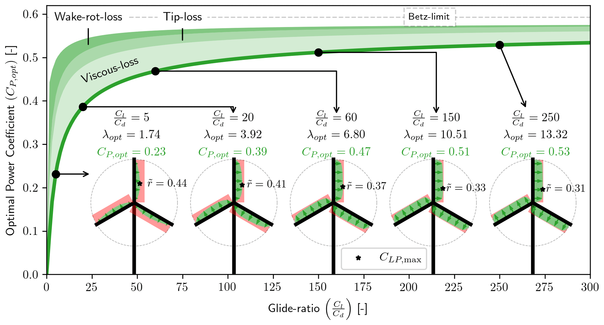
In Fig. 6 the result of solving the optimization problem for optimal tip speed ratio with varying spanwise constant glide ratio is shown. As expected, the optimal tip speed ratio is seen to increase as the glide ratio increases due to the balance between the viscous losses (increases with increasing λ) and wake rotation losses as well as tip losses (decreases with increasing λ). It is interesting to note the significant impact of including tip loss on λ_opt, with the inclusion of tip loss leading to a larger λ_opt. Four points along the λ_opt curve in Fig. 6 are highlighted, showing diagrams of the local thrust and local power with the difference to the Betz–Joukowsky limit shown by the shaded red region.

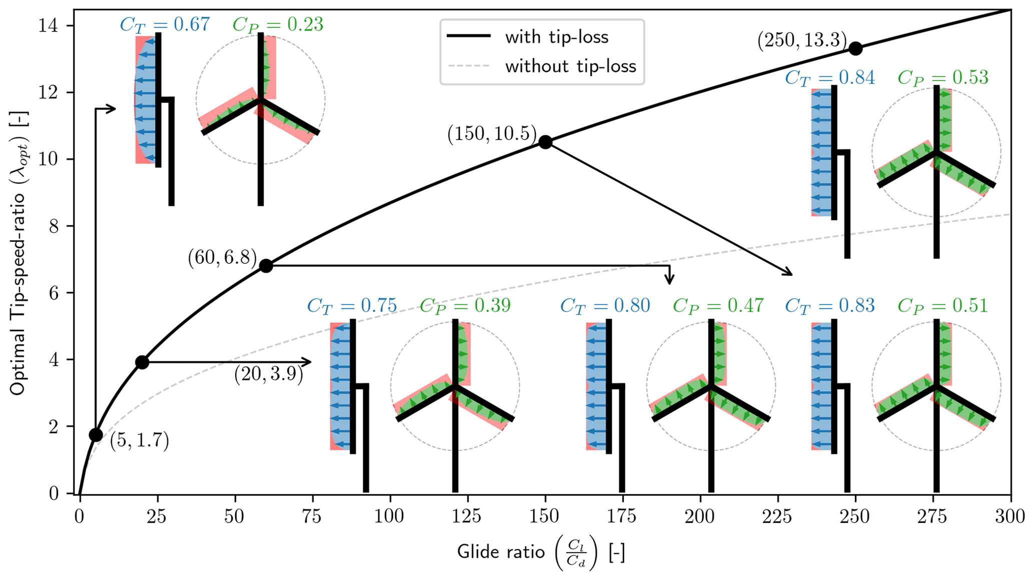
Figure 6 Optimal tip speed ratio (λ_opt) vs. spanwise constant glide ratio ($\frac{C_{\mathrm{l}}}{C_{\mathrm{d}}}$) both with and without tip loss included in the optimization. For the case with tip loss included, five points are highlighted, showing diagrams of the local thrust (C_LT) and the local power (C_LP).

The associated C_P,opt is shown in Fig. 7. The three power loss contributions are shown as shaded regions, and the viscous loss is seen to be the most significant regardless of the glide ratio. Tip loss is seen to be the second most significant loss, at least for $\frac{C_{\mathrm{l}}}{C_{\mathrm{d}}}>\mathrm{25}$, which anyway would be a very low value for a modern utility scale wind turbine. The slope of C_P,opt is seen to become flat for large values of the glide ratio, and the improvement in C_P,opt from $\frac{C_{\mathrm{l}}}{C_{\mathrm{d}}}=\mathrm{100}$ to $\frac{C_{\mathrm{l}}}{C_{\mathrm{d}}}=\mathrm{150}$ is $\mathrm{\Delta }{C}_{\mathrm{P},\mathrm{opt}}=\mathrm{3.5}$ %, and that is with a glide ratio improvement of $\mathrm{\Delta }\frac{C_{\mathrm{l}}}{C_{\mathrm{d}}}=\mathrm{50}$ %.

Figure 7 Optimal power coefficient (C_P,opt) vs. spanwise constant glide ratio ($\frac{C_{\mathrm{l}}}{C_{\mathrm{d}}}$). The same five points as in Fig. 6 are highlighted, but only the local power (C_LP) is shown for the diagrams with the addition of the point of max local power (C_LP,max).

3.4 Compared to other work

The results of C_P maximization presented in Figs. 5–7 are not in themselves novel results. Similar results have been shown by Wilson et al. (1976, Sect. 3.1–2), Manwell et al. (2010, Sect. 3.9), Sørensen (2016, chap. 5) and Jamieson (2018, Sect. 1.9). The novelty is the ease with which these results can be obtained and the extent to which this method can be applied. In all of the mentioned works, the optimization method relies on excluding mechanisms like rotational effects, drag, or tip loss or an assumption of constant axial induction to find a solution without the use of an optimizer. For Wilson et al. (1976), Manwell et al. (2010) and Sørensen (2016) drag is excluded for the induced velocity as was also done within this paper. However, the reason to exclude drag from the induced velocity within this paper is for the derivation of RIAD to be simpler. Including drag in the induced velocity will make Eq. (19) more complicated, but the optimization methods presented in Set. 3.2 and 3.3 would still be applicable. A large part of why RIAD is easy to use and implement for optimization is the use of the complex step method, which is arguably not an invention of RIAD, and it could as well be applied for a regular BEM, with the same result, although the optimization would be more convoluted. RIAD is established on a better BEM parametrization dedicated to optimization when solving load-constrained power optimizations as is shown in Part 2 of this paper (Loenbaek et al., 2021).

4 From RIAD to rotor blade planform

Section 2.3 presented the connection between inputs, such as local thrust, tip speed ratio and glide ratio, for rotor power performance, and Sect. 3.2 and 3.3 presented the power optimization. But the presented methods only contain information about the loading and power at the actuator disc, where this section establishes the connection between the RIAD inputs and the blade planform, such as blade chord and twist. The blade planform is then used as an input for a BEM solver to validate that RIAD and BEM are equivalent formulations.

4.1 Equations for chord and twist

An equation for chord can be found from Eq. (13) while applying the closure equations (Eqs. 17 and 18) for cos ϕ, resulting in the following:

$$\begin{array}{}\text{(36)}& \begin{array}{rl}c& \left(C_{\mathrm{LT}},\stackrel{\mathrm{̃}}{r},\mathit{\lambda },C_{\mathrm{l}},R,B\right)={\displaystyle \frac{\mathrm{8}\mathit{\pi }\stackrel{\mathrm{̃}}{r}R{C}_{\mathrm{LT}}}{B{C}_{\mathrm{l}}}}{\displaystyle \frac{\mathrm{1}}{\mathit{\lambda }\stackrel{\mathrm{̃}}{r}+\sqrt{{\mathit{\lambda }}^{\mathrm{2}}{\stackrel{\mathrm{̃}}{r}}^{\mathrm{2}}+\frac{C_{\mathrm{LT}}}{F}}}}\\ & {\displaystyle \frac{\mathrm{1}}{\sqrt{{\left(\mathrm{1}+\sqrt{\mathrm{1}-\frac{C_{\mathrm{LT}}}{F}}\right)}^{\mathrm{2}}+{\left(\mathit{\lambda }\stackrel{\mathrm{̃}}{r}+\sqrt{{\mathit{\lambda }}^{\mathrm{2}}{\stackrel{\mathrm{̃}}{r}}^{\mathrm{2}}+\frac{C_{\mathrm{LT}}}{F}}\right)}^{\mathrm{2}}}}}.\end{array}\end{array}$$

To compute the chord it is seen that additional inputs are required, such as lift coefficient (C_l), the number of blades (B) and rotor radius (R).

An equation for twist can be found in much the same way by using Eq. (16) for tan ϕ and applying the closure equations. Combining it with $\mathit{\varphi }=\mathit{\alpha }+{\mathit{\theta }}_{\mathrm{twist}}+{\mathit{\theta }}_{\mathrm{pitch}}$, the following equation for the twist can be found:

$$\begin{array}{}\text{(37)}& \begin{array}{rl}{\mathit{\theta }}_{\mathrm{twist}}\left(C_{\mathrm{LT}},\stackrel{\mathrm{̃}}{r},\mathit{\lambda }\right)=& \underset{\mathit{\varphi }}{\underbrace{{\tan }^{-\mathrm{1}}\left({\displaystyle \frac{\mathrm{1}+\sqrt{\mathrm{1}-\frac{C_{\mathrm{LT}}}{F}}}{\mathit{\lambda }\stackrel{\mathrm{̃}}{r}+\sqrt{{\mathit{\lambda }}^{\mathrm{2}}{\stackrel{\mathrm{̃}}{r}}^{\mathrm{2}}+\frac{C_{\mathrm{LT}}}{F}}}}\right)}}\\ & -\mathit{\alpha }-{\mathit{\theta }}_{\mathrm{pitch}}.\end{array}\end{array}$$

4.2 Validation with BEM

To show that RIAD is an equivalent formulation of the BEM equations, a planform design is created through Eqs. (36) and (37) and evaluated with a BEM solver. The BEM solver used for the validation is CCBlade (Ning, 2014).

Running CCBlade requires an airfoil polar (C_l, C_d vs. α), and to keep it as simple as possible a single airfoil polar is used all along the blade span. The airfoil is taken to be FFA-W3-301 (Bjorck, 1990) with the aerodynamic data from Bak et al. (2013) ($Re=\mathrm{10}\times {\mathrm{10}}^{\mathrm{6}}$). The design point for the polar was for simplicity taken as the angle of attack with maximum glide ratio, resulting in the following:

$$\begin{array}{}\text{(38)}& {\displaystyle }& {\displaystyle \frac{C_{\mathrm{l}}}{C_{\mathrm{d}}}}=\mathrm{92},\text{(39)}& {\displaystyle }& {\displaystyle }\mathit{\alpha }=\mathrm{10.6}{}^{\circ },\text{(40)}& {\displaystyle }& {\displaystyle }{C}_{\mathrm{l}}=\mathrm{1.52}.\end{array}$$

Running the optimization for λ_opt as described in Sect. 3.3 gave λ_opt=8.4, which is the tip speed ratio used for the design. To give the design some real dimensions, a rotor radius of R=50 m is used.

The resulting planform design can be seen in Fig. 8. Using the planform design as input for CCBlade as well as the other inputs, the resulting local thrust and local power were found from CCBlade. A comparison between RIAD and CCBlade can be seen in Fig. 9. Figure 9a shows the values for C_LT and C_LP for both the solvers. Figure 9b shows the difference between RIAD and CCBlade for both C_LT and C_LP using a log scale on the y axis, both as a function of the normalized radius. In the root region the two methods are seen to agree to machine precision but with an error that is growing towards the tip and reaching a difference of 10⁻⁴ (which is still three significant digits). The growing error is found to disappear if tip loss is excluded (agrees to machine precision), and the difference is also seen to disappear if the drag is included for the induction as well as including the tip loss. The difference is therefore attributed to some small implementation difference regarding the tip loss, but as the difference is anyway insignificant, the difference is not investigated any further. It should be noted that for the comparison with CCBlade, it is C_LT,blade that is used, where C_LT,blade was discussed in Sect. 2.6.

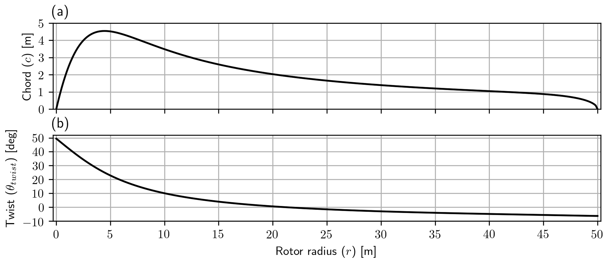
Figure 8 (a) Blade chord and (b) blade twist both as a function of radius. The number of blades is assumed to be B=3.

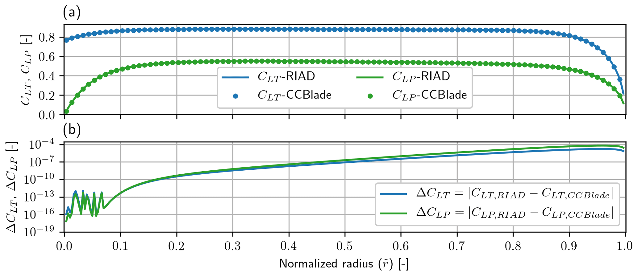
Figure 9 (a) Local thrust (C_LT) and local power (C_LP) for RIAD (line) and CCBlade (dots). (b) The difference between the two methods for local thrust (ΔC_LT) and local power (ΔC_LP). The difference is seen to increase towards the tip, but the agreement is still within three significant digits and is therefore thought to be insignificant. The difference is likely a small implementation difference within tip loss modeling.

5 Conclusion

A rotor performance model called the Radially Independent Actuator Disc (RIAD) model was presented. It is a different parametrization of the blade element momentum (BEM) equations which is found to be better for wind turbine optimization. The model relates the local rotor power output (local-power coefficient – C_LP) to the local rotor loading input (local-thrust coefficient – C_LT) at a given radial station ($\stackrel{\mathrm{̃}}{r}$). The model is a simple equation, shown in Eq. (19), from which different physical effects can easily be interpreted, such as wake rotation loss, tip loss and viscous loss.

A method to compute gradients for RIAD was presented, through the use of the complex step method, which allows us to compute the gradient to machine precision with minimum additional work required.

The gradients were used for classical power coefficient (C_P) maximization, which was first applied for loading optimization (C_LT along the span) for a given tip speed ratio and glide ratio. The optimization was then extended for the combined optimization of the tip speed ratio and loading, leading to a nested optimization for C_P which only requires the glide ratio along the span as an input. Using a spanwise constant glide ratio it was shown that viscous loss is the most significant loss, regardless of the value of the glide ratio. The optimization results by themselves have been done before, but the novel development is the ease with which the optimal result can be achieved and the extent to which the method can be applied. But the real strength of using RIAD for optimization is for load constraint rotor optimization as described in Part 2 (Loenbaek et al., 2021).

The relationship between local thrust along the span and the blade chord and twist was presented, and they were used to create the input for validation with a BEM solver (Ning, 2014). The difference between the two methods was found to agree to three significant digits with a likely small implementation difference for the tip loss modeling. In this way, it was shown that RIAD and BEM are equivalent, with the difference being the parametrization.

Appendix A: Nomenclature

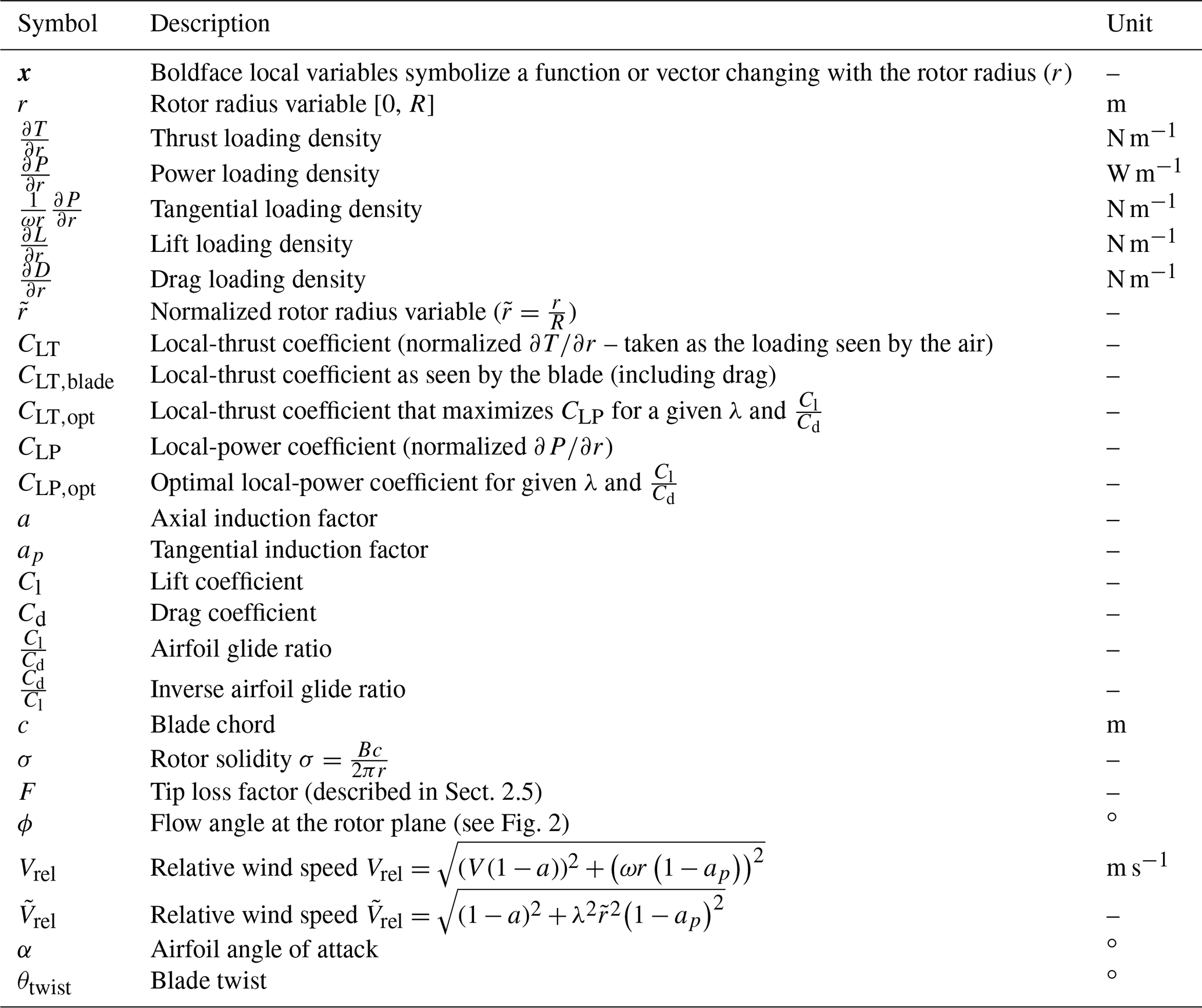
A1 Rotor local variables

Table A1 Variables that are scalars at a given radius location (r). Boldface variables indicate a function or vector changing with radius.

A2 Rotor global variables

Table A2 Variables that are scalars for the whole rotor.